PairMotif+: A Fast and Effective Algorithm for De Novo Motif Discovery in DNA sequences

Int. J. Biol. Sci. 2013, Vol. 9

http://www.ijbs.com

412

IInntteerrnnaattiioonnaall JJoouurrnnaall ooff BBiioollooggiiccaall SScciieenncceess 2013; 9(4):412-424. doi: 10.7150/ijbs.5786

Research Paper

PairMotif+: A Fast and Effective Algorithm for De Novo Motif Discovery in DNA sequences Qiang Yu, Hongwei Huo, Yipu Zhang, Hongzhi Guo, Haitao Guo

School of Computer Science and Technology, Xidian University, Xi’an, 710071, China.

Corresponding author: Prof. Hongwei Huo, School of Computer Science and Technology, Xidian University, Xi’an, 710071, China. Phone: 86-29-88201489, Fax: 86-29-88201489, E-mail: [email protected].

© Ivyspring International Publisher. This is an open-access article distributed under the terms of the Creative Commons License (http://creativecommons.org/ licenses/by-nc-nd/3.0/). Reproduction is permitted for personal, noncommercial use, provided that the article is in whole, unmodified, and properly cited.

Received: 2013.01.01; Accepted: 2013.04.15; Published: 2013.04.29

Abstract

The planted (l, d) motif search is one of the most widely studied problems in bioinformatics, which plays an important role in the identification of transcription factor binding sites in DNA sequences. However, it is still a challenging task to identify highly degenerate motifs, since current algorithms either output the exact results with a high computational cost or accomplish the computation in a short time but very often fall into a local optimum. In order to make a better trade-off between accuracy and efficiency, we propose a new pattern-driven algorithm, named PairMotif+. At first, some pairs of l-mers are extracted from input sequences according to probabilistic analysis and statistical method so that one or more pairs of motif instances are included in them. Then an approximate strategy for refining pairs of l-mers with high accuracy is adopted in order to avoid the verification of most candidate motifs. Experimental results on the simulated data show that PairMotif+ can solve various (l, d) problems within an hour on a PC with 2.67 GHz processor, and has a better identification accuracy than the compared algorithms MEME, AlignACE and VINE. Also, the validity of the proposed algorithm is tested on multiple real data sets.

Key words: Motif search; Transcription factor binding sites; Pattern-driven algorithms.

Introduction DNA motifs refer to short DNA segments that

are regulatory elements bound by proteins such as transcription factors. Motif discovery is to find the unknown motifs in the given sequences, which plays an important role in locating transcription factor binding sites (TFBSs) in DNA sequences. The planted (l, d) motif search (PMS) [1], which is raised from this research, has become a widely accepted motif search problem formulation.

Problem Definition. Given a set of n-length se-quences S = {sl, s2, … , st} over the alphabet {A, G, C, T} and nonnegative integers l and d, satisfying 0 ≤ d < l < n. The PMS problem is to find an l-mer (i.e., an l-length string) m, such that each sequence si contains an l-mer mi differing from m in at most d positions. The l-mer m is called an (l, d) motif and each mi is

called an instance of m. The PMS problem is NP-hard [2]. With t and n

fixed, different values of l and d form various PMS instances. Usually, the motif length l is 5 to 25 base-pairs (bps). For a given motif length l, the larger the degenerate positions d, the more difficult it is to iden-tify the planted (l, d) motif in input sequences. Specif-ically, some researchers [3, 4] use 2d-neighborhood probability (i.e., the probability that the Hamming distance between two random l-mers is not larger than 2d) to measure the difficulty of solving different PMS instances, since it is a good indicator to reflect the degree of degeneracy of PMS instances [3].

The algorithms for PMS are categorized as ap-proximate and exact depending on whether they are guaranteed to find the optimal motif always or not [5].

Ivyspring

International Publisher


http://www.ijbs.com

413

The approximate algorithms, which commonly model motifs using position weight matrix (PWM), can re-port results in a short time but not guarantee a global optimum. Most approximate recognition algorithms use potent statistical techniques. For example, the most popular algorithms MEME [6] and Gibbs Sam-pling [7] adopt Expectation Maximization (EM) and Gibbs sampling techniques, respectively. Based on MEME, there are the extension algorithms, like PROJECTION [1] and GADEM [8]. PROJECTION partitions all l-mers in S into many buckets and selects some valid buckets that contain several occurrences of the desired motif and little else, in order to provide a good initial state for the EM refinement. GADEM employs a genetic algorithm with an embedded EM algorithm to improve initial PWMs. The modification of Gibbs Sampling is described in [9-11]. In recent years, Bayesian theory has also been introduced in the field of motif search, such as BayesMD [12], A-GLAM [13], SBaSeTraM [14] and BAMBI [15]. Besides the statistical methods, some graph-theoretic methods either based on clustering or on heuristic search are proposed to solve the motif search problem, such as MotifCut [16], sMCL-WMR [17] and Vine [18]. In the associated graphical model, each node corresponds to an l-mer in input sequences and each edge represents the similarity between the two l-mers it connects.

Exact recognition algorithms, which use con-sensus to represent motifs, find all (l, d) motifs and the optimal one by traversing the whole search space. Since all exact algorithms produce the consistent re-sults [19], the main concern on them is the time per-formance. Based on the graphical model of motif search, some exact algorithms, such as DPCFG [20] and RecMotif [4], find all maximum cliques in the graph, with a search space of O(nt). The time perfor-mance of these algorithms does not depend on the motif length, but it is difficult for these algorithms to identify highly degenerate motifs because the associ-ated graphs are so dense that numerous cliques need to be verified. There are some other exact algorithms based on pattern-driven. They verify all string pat-terns of length l, and output the patterns that occur in all input sequences with at most d mutations. The initial search space of these algorithms, O(4l), is much smaller than O(nt). Therefore, the recent research of exact recognition algorithms mainly concentrates on the pattern-driven algorithms, including the series of suffix tree algorithms [21-24] and the series of PMS algorithms [5, 25-28]. Pattern-driven algorithms are good at finding motifs of length smaller than 20 bps, but their time overhead or space requirement will become unrealistic with the increase of the motif length.

Although many recognition algorithms have

been proposed to solve the PMS problem, few of them can make a good trade-off between accuracy and time performance. In identifying highly degenerate motifs, they either output the exact results with a high com-putational cost or accomplish the computation in a short time but have a low accuracy. Thus, it is a meaningful work to design an algorithm that can get high accuracy results within a reasonable time, e.g., an hour on personal computers. To achieve this goal, we propose a new algorithm named PairMotif+, by de-signing the approximate version of PairMotif [29]. PairMotif, our recent exact algorithm, adopts the fol-lowing idea: select multiple pairs of l-mers in which there must exist a pair of motif instances, by travers-ing reference sequences; then, refine each pair of l-mers, namely verify whether each d-neighbor of the pair of l-mers is a valid (l, d) motif. Obviously, the time performance of PairMotif depends on two val-ues: the number of the selected pairs of l-mers and the number of the candidate motifs generated from each pair of l-mers.

The main idea of PairMotif+ is to reduce the above two values that determine the time perfor-mance. PairMotif+ consists of three steps. First, extract some pairs of l-mers from input sequences according to probabilistic analysis so that more than half of the pairs of motif instances are included in them. Second, analyze the weights of the extracted pairs of l-mers and filter out the pairs with small weights, ensuring at least one pair of motif instances are included in the remaining pairs of l-mers. Third, in refining each pairs of l-mers, use an approximate strategy with high ac-curacy to avoid the verification of most candidate motifs. Experimental results show that PairMotif+ can solve various PMS instances within an hour on a PC with 2.67 GHz processor, and outperforms the com-petition in identification accuracy.

Methods Foundations

In our recent work [29], we discussed how to partition and traverse the d-neighbors (candidate mo-tifs) shared by a pair of l-mers, which is the basic of refining pairs of l-mers in this paper. This section provides a brief description of the partition and trav-ersing methods.

Definition 1. Given a pair of l-mers x1 and x2, the common d-neighbors (candidate motifs), Md(x1, x2), is defined to be {y: |y| = l, dH(y, x1) ≤ d and dH(y, x2) ≤ d}, where dH(·) denotes the Hamming distance between two l-mers.

Definition 2. Given a pair of l-mers x1 and x2 and another l-mer y, the l positions in the alignment of these three l-mers can be divided into four categories:


http://www.ijbs.com

414

P00(x1, x2, y), P01(x1, x2, y), P10(x1, x2, y) and P11(x1, x2, y). For each position i (1 ≤ i ≤ l), assume that it belongs to Pab(x1, x2, y). Then, a is 1 if x1[i] = x2[i], 0 otherwise; b is 1 if either y[i] = x1[i] or y[i] = x2[i], 0 otherwise. Fig. 1 shows an example for partitioning the positions in the alignment of three l-mers.

Fig. 1 An example for partitioning positions in the alignment of three l-mers.

Definition 3. Given a pair of l-mers x1 and x2 and

another l-mer y ∈ Md(x1, x2), the mapping relation from x1 and x2 to y, R(x1, x2, y), is defined to be a 2-tuple <|P10(x1, x2, y)|, |P00(x1, x2, y)|>. Furthermore, the mapping relation from x1 and x2 to Md(x1, x2), R(x1, x2), is defined to be

…(1)

Given a pair of l-mers x1 and x2, the elements in R(x1, x2) implies the approach to partitioning and traversing the candidate motif set Md(x1, x2). We first discuss how to compute R(x1, x2). For any candidate motif y in Md(x1, x2), let R(x1, x2, y) = <α, β>. From Definition 2 and 3, α represents the number of posi-tions at which x1[·] = x2[·], y[·] ≠ x1[·] and y[·] ≠ x2[·]; β represents the number of positions at which x1[·] ≠ x2[·], y[·] ≠ x1[·] and y[·] ≠ x2[·]. Thus, we have 0 ≤ α ≤ l - dH(x1, x2), 0 ≤ β ≤ dH(x1, x2) and dH(y, x1) + dH(y, x2) = 2α + 2β + (dH(x1, x2) -β). Furthermore, we have dH(y, x1) + dH(y, x2) ≤ 2d because y is the d-neighbor of both x1 and x2. Based on these considerations, we obtain inequali-ties (2). Obviously, the values of α and β are deter-mined by dH(x1, x2), and R(x1, x2) can be calculated by listing all 2-tuples <α, β> satisfying (2). For example, for the PMS instance (15, 4), R(x1, x2) = {<0, 0>, <0, 1>, <0, 2>, <0, 3>, <0, 4>, <1, 0>, <1, 1>, <1, 2>, <2, 0>} when dH(x1, x2) = 4.

…(2)

Based on the different 2-tuples in R(x1, x2), the candidate motif set Md(x1, x2) can be partitioned to |R(x1, x2)| mutually disjoint subsets. For each <α, β>

in R(x1, x2), the corresponding subset of Md(x1, x2) is denoted by Md<α, β>(x1, x2), namely Md<α, β>(x1, x2) = {y: y∈Md(x1, x2) and R(x1, x2, y) = <α, β>}. Assume that <α, β> and <α', β'> are two different elements of R(x1, x2), then we have Md<α, β>(x1, x2) ∩ Md<α', β'>(x1, x2) = Ф ac-cording to Definition 3. Since R(x1, x2) represents the mapping relation from x1 and x2 to all candidate mo-tifs, the partition of Md(x1, x2) is:

Md(x1, x2) = {Md<α, β>(x1, x2): <α, β>∈R(x1, x2)} …(3)

In terms of equation (3), we can traverse the candidate motifs derived from x1 and x2, by generat-ing the mutually disjoint subsets of Md(x1, x2) one by one. For each <α, β> in R(x1, x2), the candidate motifs in Md<α, β>(x1, x2) are generated as follows. First, set the initial candidate motif y as x2. Second, select α posi-tions from the positions at which x1[·] = x2[·], and for each of these α positions, change y[·] to one of the three characters different from x1[·]. Third, select β positions from the positions at which x1[·] ≠ x2[·], and for each of these β positions, change y[·] to one of the two characters different from x1[·] and x2[·]. Fourth, select a part of positions from the positions at which x1[·] ≠ x2[·] except for those selected in the previous step, and change y[·] to x1[·] for each of these posi-tions. More details about these steps can be found in the reference [29]. According to the process of gener-ating candidate motifs, the size of Md<α, β>(x1, x2) is calculated by (4) where dH denotes the Hamming distance between x1 and x2.

…(4)

Step 1: Extracting Pairs of l-mers PairMotif+ only extracts the pair of l-mers that

contains two l-mers x1 and x2 coming from different sequences, i.e., x1∈l si, x2 ∈l sj and i ≠ j. Thus, the pair of l-mers x1 and x2 can be denoted by (x1, x2) if i < j, (x2, x1) otherwise. The set of all pairs of l-mers in input sequences S is denoted by L = {(x1, x2): (∀i, j)(1 ≤ i < j ≤ t, x1∈l si and x2∈l sj)}.

The aim of Step 1 is to extract as few pairs of l-mers as possible from L, and ensure that sufficient (more than half of) pairs of motif instances are in-cluded in them. We set a threshold k (0 ≤ k ≤ l), and then extract the pairs of l-mers (x1, x2) from L with dH(x1, x2) ≤ k. The set of the extracted pairs of l-mers is denoted by L1={(x1, x2): (x1, x2)∈L and dH(x1, x2) ≤ k}.

For a proper choice of the threshold k, we con-sider two probabilities. One is the probability that the Hamming distance between two random l-mers is less than or equal to k, denoted by pk. The other is the probability that the Hamming distance between two

),(

212121

)},,({),(xxMy d

yxxRxxR∈

=

≤≤−≤≤

≤++

).,(0),,(0

,2),(2

21

21

21

xxdxxdl

dxxd

H

H

H

βαβα

∑−−≤≤−+

−≤≤><

−××

××

−=

βααβ

βαβα

ββα

HH

Hdidd

di

HHHd i

dddlxxM

,021, 23),(


http://www.ijbs.com

415

randomly selected motif instances is less than or equal to k, denoted by p'k. The probability pk is calculated by (5).

…(5)

In order to calculate p'k, given a motif m and a motif instance m', more specific distance relation be-tween m and m' is required besides 0 ≤ dH(m, m') ≤ d. We determine this relation by assuming that m' is ob-tained from m as follows: select d positions in m at random, and then replace each character at the se-lected positions with a random character in {A, G, C, T}. Since each of the selected d positions is changed with probability 3/4, the expectation of the distance between m and m' is 3d/4, the rationality of which will be analyzed in Discussion and Conclusions. On this basis, the probability that the Hamming distance be-tween m and m' is k (0 ≤ k ≤ d) can be calculated by (6).

…(6)

Let m1 and m2 be two randomly selected in-stances of the motif m. <dH(m, m1), dH(m, m2)> repre-sents the distance between m and the pair of motif instances (m1, m2), corresponding to a sample space Ω = {<i, j>: 0 ≤ i ≤ d, 0 ≤ j ≤ d }. Let P(<i, j>) denote the probability of <dH(m, m1), dH(m, m2)> = <i, j>. As dH(m, m1) = i and dH(m, m2) = j are independent with each other, we have:

P(<i, j>) = P(dH(m, m1) = i) × P(dH(m, m2) = j) …(7)

Based on the above equations, p'k can be calcu-lated using the Theorem of Total Probability:

…(8)

In (8), P(dH(m1, m2) ≤ k | <i, j>) represents the probability of dH(m1, m2) ≤ k given <dH(m, m1), dH(m, m2)> = <i, j>. Its value can be calculated according to the actual situation. For example, for the PMS instance (15, 4), P(dH(m1, m2) ≤ 4 | <2, 2>) = 1, and

With p'k, it is easy to calculate the expectation of the number of extracted pairs of motif instances E[Nm]. For the PMS problem, each input sequence contains a motif instance, so there are totally t(t-1)/2 pairs of motif instances. Moreover, in extracting pairs of l-mers with the restriction of the threshold k, each pair of motif instances has a probability of p'k to be

extracted. Therefore,

E[Nm] = t(t-1)/2 × p'k …(9)

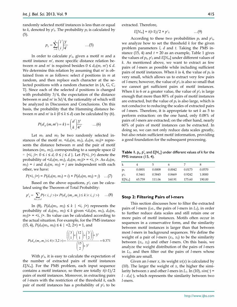
According to these two probabilities pk and p'k, we analyze how to set the threshold k for the given problem parameters l, d and t. Taking the PMS in-stance (15, 4) and t = 20 as an example, Table 1 gives the values of pk, p'k and E[Nm] under different values of k. As mentioned above, we want to extract as few pairs of l-mers as possible while including sufficient pairs of motif instances. When k is 4, the value of pk is very small, which allows us to extract very few pairs of l-mers; however, the value of p'k is also so small that we cannot get sufficient pairs of motif instances. When k is 6 or a greater value, the value of p'k is large enough that more than 80% of pairs of motif instances are extracted, but the value of pk is also large, which is not conducive to reducing the scales of extracted pairs of l-mers. Therefore, it is appropriate to set k as 5 to perform extraction: on the one hand, only 0.08% of pairs of l-mers are extracted; on the other hand, nearly 60% of pairs of motif instances can be extracted. In doing so, we can not only reduce data scales greatly, but also retain sufficient motif information, providing a good foundation for the subsequent processing.

Table 1. pk, p'k and E[Nm] under different values of k for the PMS instance (15, 4).

k 4 5 6 7 8 pk 0.0001 0.0008 0.0042 0.0173 0.0570 p'k 0.3461 0.5845 0.8469 0.9242 1.0000 E[Nm] 65.759 111.06 160.91 175.60 190.00

Step 2: Filtering Pairs of l-mers This section discusses how to filter the extracted

pairs of l-mers (i.e., the pairs of l-mers in L1), in order to further reduce data scales and still retain one or more pairs of motif instances. Motifs often occur in sequences in a conservative form, and the similarity between motif instances is larger than that between most l-mers in background sequences. We define the weight of a pair of l-mers (x1, x2) to be the similarity between (x1, x2) and other l-mers. On this basis, we analyze the weight distribution of the pairs of l-mers in L1, and then filter out the pairs of l-mers whose weights are small.

Given an l-mer x, its weight w(x) is calculated by (10). The larger the weight of x, the higher the simi-larity between x and other l-mers in L1. In (10), sim(·) = l - dH(·), which represents the similarity between two l-mers.

∑=

=

k

il

i

k il

p0 4

3

d

k

H kd

kmmdP43))',((

==

∑≤≤

><≤×><=dji

Hk jikmmdPjiPp,0

21 ),|),((),('

371.03

215

323

112

13

)2,3|4),((2

2

21 =×

×

+

×

=><≤mmdP H


http://www.ijbs.com

416

…(10)

Based on (10), the weight of a pair of l-mers (x1, x2), w(x1, x2), is calculated as follows:

w(x1, x2) = w(x1) + w(x2) …(11)

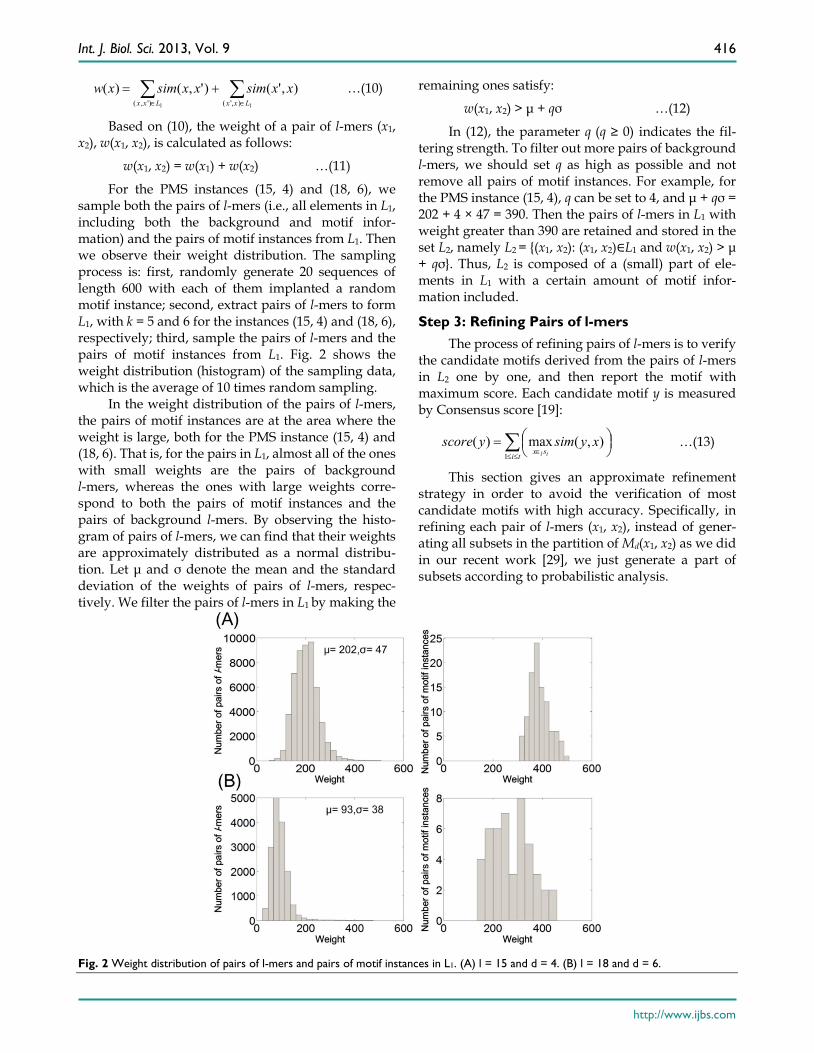
For the PMS instances (15, 4) and (18, 6), we sample both the pairs of l-mers (i.e., all elements in L1, including both the background and motif infor-mation) and the pairs of motif instances from L1. Then we observe their weight distribution. The sampling process is: first, randomly generate 20 sequences of length 600 with each of them implanted a random motif instance; second, extract pairs of l-mers to form L1, with k = 5 and 6 for the instances (15, 4) and (18, 6), respectively; third, sample the pairs of l-mers and the pairs of motif instances from L1. Fig. 2 shows the weight distribution (histogram) of the sampling data, which is the average of 10 times random sampling.

In the weight distribution of the pairs of l-mers, the pairs of motif instances are at the area where the weight is large, both for the PMS instance (15, 4) and (18, 6). That is, for the pairs in L1, almost all of the ones with small weights are the pairs of background l-mers, whereas the ones with large weights corre-spond to both the pairs of motif instances and the pairs of background l-mers. By observing the histo-gram of pairs of l-mers, we can find that their weights are approximately distributed as a normal distribu-tion. Let μ and σ denote the mean and the standard deviation of the weights of pairs of l-mers, respec-tively. We filter the pairs of l-mers in L1 by making the

remaining ones satisfy:

w(x1, x2) > μ + qσ …(12)

In (12), the parameter q (q ≥ 0) indicates the fil-tering strength. To filter out more pairs of background l-mers, we should set q as high as possible and not remove all pairs of motif instances. For example, for the PMS instance (15, 4), q can be set to 4, and μ + qσ = 202 + 4 × 47 = 390. Then the pairs of l-mers in L1 with weight greater than 390 are retained and stored in the set L2, namely L2 = {(x1, x2): (x1, x2)∈L1 and w(x1, x2) > μ + qσ}. Thus, L2 is composed of a (small) part of ele-ments in L1 with a certain amount of motif infor-mation included.

Step 3: Refining Pairs of l-mers The process of refining pairs of l-mers is to verify

the candidate motifs derived from the pairs of l-mers in L2 one by one, and then report the motif with maximum score. Each candidate motif y is measured by Consensus score [19]:

…(13)

This section gives an approximate refinement strategy in order to avoid the verification of most candidate motifs with high accuracy. Specifically, in refining each pair of l-mers (x1, x2), instead of gener-ating all subsets in the partition of Md(x1, x2) as we did in our recent work [29], we just generate a part of subsets according to probabilistic analysis.

Fig. 2 Weight distribution of pairs of l-mers and pairs of motif instances in L1. (A) l = 15 and d = 4. (B) l = 18 and d = 6.

∑∑∈∈

+=11 ),'()',(

),'()',()(LxxLxx

xxsimxxsimxw

∑≤≤

∈

=

tisx

xysimyscoreil1

),(max)(


http://www.ijbs.com

417

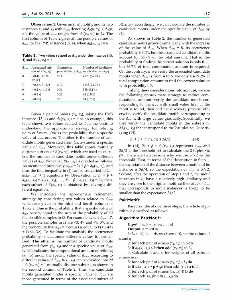
Observation 1. Given an (l, d) motif y and its two instances x1 and x2 with dsum denoting dH(y, x1) + dH(y, x2), the value of dsum ranges from dH(x1, x2) to 2d. The first column of Table 2 gives all the possible values of dsum for the PMS instance (15, 4), when dH(x1, x2) = 4.

Table 2 . Two values related to dsum under the instance (15, 4) and dH(x1, x2) = 4.

dsum Associated sub-sets of R(x1, x2)

Occurrence probability of dsum

Number of candidate motifs (Percentage)

8 {<0,4>, <1,2>, <2,0>}

0.11 4570 (66.7%)

7 {<0,3>, <1,1>} 0.19 1648 (24.0%) 6 {<0,2>, <1,0>} 0.36 558 (8.1%) 5 {<0,1>} 0.24 64 (0.9%) 4 {<0,0>} 0.10 14 (0.2%)

Given a pair of l-mers (x1, x2), taking the PMS

instance (15, 4) and dH(x1, x2) = 4 as an example, this table shows two values related to dsum, the basic to understand the approximate strategy for refining pairs of l-mers. One is the probability that a specific value of dsum occurs. The other is the number of can-didate motifs generated from (x1, x2) under a specific value of dsum. Moreover, this table shows mutually disjunct subsets of R(x1, x2), which are used to calcu-late the number of candidate motifs under different values of dsum. Note that, R(x1, x2) is divided as follows. As mentioned previously, dsum = 2α + β + dH(x1, x2), and thus the first inequality in (2) can be converted to 2d - dH(x1, x2) + 1 equations by Observation 1: 2α + β + dH(x1, x2) = dH(x1, x2), … , 2α + β + dH(x1, x2) = 2d; then, each subset of R(x1, x2) is obtained by solving a dif-ferent equation.

We introduce the approximate refinement strategy by considering two values related to dsum, which are given in the third and fourth column of Table 2. One is the probability that a specific value of dsum occurs, equal to the sum of the probability of all the possible samples in Ω. For example, when dsum = 7, the possible samples in Ω are <3, 4> and <4, 3>, and the probability that dsum = 7 occurs is equal to P(<3, 4>) + P(<4, 3>). To facilitate the analysis, the occurrence probability of dsum under different values is normal-ized. The other is the number of candidate motifs generated from (x1, x2) under a specific value of dsum, which indicates the computational amount of refining (x1, x2) under the specific value of dsum. According to different values of dsum, R(x1, x2) can be divided into 2d - dH(x1, x2) + 1 mutually disjunct subsets, as shown in the second column of Table 2. Thus, the candidate motifs generated under a specific value of dsum are those generated in terms of the associated subset of

R(x1, x2); accordingly, we can calculate the number of candidate motifs under the specific value of dsum by (4).

As shown in Table 2, the number of generated candidate motifs grows dramatically with the increase of the value of dsum. When dsum = 8, its occurrence probability is 0.11, but the associated candidate motifs account for 66.7% of the total amount. That is, the probability of finding the correct solution is only 0.11, but 66.7% of total computation amount is required. On the contrary, if we verify the associated candidate motifs when dsum is from 4 to 6, we only use 9.2% of total computation amount to find the correct solution with probability 0.7.

Taking these considerations into account, we use the following approximate strategy to reduce com-putational amount: verify the candidate motifs cor-responding to the dsum with small value first. If the motif is found, then end the discovery process; oth-erwise, verify the candidate motifs corresponding to the dsum with large values gradually. Specifically, we first verify the candidate motifs in the subsets of Md(x1, x2) that correspond to the 2-tuples <α, β> satis-fying (14).

2α + β + dH(x1, x2) ≤ 3d/2 …(14)

In (14), 2α + β + dH(x1, x2) represents dsum, and 3d/2 is the threshold set to calculate the 2-tuples <α, β>. There are two reasons why we use 3d/2 as the threshold. First, in terms of the description in Step 1, the expectation of the distance between a motif and its instance is 3d/4, so the expectation of dsum is 3d/2. Second, after the operation of Step 1 and 2, the motif instances in L2 have a relatively high similarity and they are close to the original motif, so the value of dsum that corresponds to motif instances is likely to be smaller than the expectation 3d/2.

PairMotif+ Based on the above three steps, the whole algo-

rithm is described as follows:

Algorithm PairMotif+ Input: l, d, S = {s1, s2, … , st} Output: a motif m 1: L1 ← Ф, L2 ← Ф, maxScore ← 0, set the values of

k and q 2: for each pair of l-mers (x1, x2) in S do 3: if dH(x1, x2) ≤ k then add (x1, x2) to L1 4: Calculate μ and σ for weights of all pairs of

l-mers in L1 5: for each pair of l-mers (x1, x2) ∈L1 do 6: if w(x1, x2) > μ + qσ then add (x1, x2) to L2 7: for each pair of l-mers (x1, x2) ∈ L2 do 8: for each <α, β> ∈R(x1, x2) do


http://www.ijbs.com

418

9: if 2α + β + dH(x1, x2) ≤ 3d/2 then 10: for each y ∈ Md<α, β>(x1, x2) do 11: if score(y) > maxScore then 12: m ← y, maxScore = score(y) 13: Output m Line 1 carries out the initialization. The values of

k and q, which depend largely on l and d, are set ac-cording to the probabilistic analysis and statistical method described in Step 1 and 2, and their values under different (l, d) instances will be given in Results section. Lines 2 - 3, which are Step 1, extract pairs of l-mers from input sequences S with the restriction of the threshold k and store them in L1. Lines 4 - 6, which perform Step 2, filter the pairs of l-mers in L1 accord-ing to the filtering strength q with remaining ones stored in L2. Lines 7 - 13, which correspond to Step 3, verify each candidate motif derived from the pairs of l-mers in L2 and output the motif with maximum score.

The time complexity of PairMotif+ depends mainly on Step 3 (lines 7 - 13). First, let N denote the number of pairs of l-mers in L2, whose order of mag-nitude is 102 or 103 in terms of the analysis in Step 2 and our experimental verification; since N is ap-proximately equal to the sequence length n, we re-place N with n in the time complexity. Second, for each pair of l-mers (x1, x2) in L2, the approximate re-finement strategy makes the distance from a candi-date motif to x1 or x2 usually less than or equal to 3d/4, and thus the probability that a random l-mer y becomes a candidate motif is Prob.[dH(y, x1) ≤ 3d/4 & dH(y, x2) ≤ 3d/4] = p23d/4; furthermore, the number of candidate motifs derived from (x1, x2) is approxi-mately equal to 4lp23d/4, where 4l is the number of all possible l-mers. Third, verifying each candidate motif y is to compare y with O(tn) l-mers in input sequences. Therefore, the expected time complexity of PairMotif+ is O(tn24l p23d/4).

The memory usage of PairMotif+ will reach its peak when Step 1 is being processed; accordingly, the space complexity of PairMotif+ depends on the number of pairs of l-mers in L1. There are a total of O(t2n2) pairs of l-mers in S and each pair has a proba-bility of pk to be extracted, so the number of pairs of l-mers in L1 is O(t2n2pk). Note that, the memory usage in refining each pair of l-mers is negligible, because PairMotif+ does not generate the whole candidate motif set in Step 3. Actually, in traversing the candi-date motif set, the algorithm verifies each candidate motif y immediately after y is generated, and then releases the associated storage space. Therefore, the space complexity of PairMotif+ is O(t2n2pk).

Results Test on Simulated Data

Simulated data provide quantitative measures to compare the performance of PairMotif+ with the ex-isting algorithms. We generate the simulated data sets following [1]: generate a motif of length l and t iden-tically distributed sequences of length n; then, for each sequence s, implant a random motif instance, which differs from the motif in at most d positions, to a random position in s. To evaluate the prediction ac-curacy, we use the nucleotide level performance coef-ficient (nPC) following [30], namely |K∩P|/|K∪P|, where K is the set of nucleotide positions corre-sponding to motif occurrences and P is the set of pre-dicted nucleotides positions.

Several representative algorithms are selected to compare with PairMotif+, including MEME [6], AlignACE [10], VINE [18] and PairMotif [29]. MEME and AlignACE are the most popular motif recognition algorithms based on PWM; they were also involved in a comparison of different recognition algorithms in the review articles [30] and [31]. Vine, a recent meth-od, is a polynomial-time heuristic algorithm based on graphical model, outperforming widely used ap-proximate algorithms on the simulated data. PairMo-tif is a fast exact algorithm, capable of reporting all (l, d) motifs; its prediction accuracy is obtained by eval-uating the (l, d) motif with maximum score. All algo-rithms are performed in the same experimental envi-ronment with a 2.67 GHz processor and a 4 Gbyte memory. The experimental results are the average derived by executing algorithms on five simulated data sets.

First, the comparisons are carried out on differ-ent PMS instances with fixed t = 20 and n = 600. As described above, 2d-neighborhood probability (p2d), which can be calculated by (5), reflects the degree of degeneracy of a PMS instance. We select ten PMS in-stances with different value of p2d as follows: l is less than or equal to 25, conforming to the general motif length; d is selected by setting the value of p2d from 0.05 to 0.7, where 0.05 is approximately equal to the p2d value of the classical PMS instance (15, 4), and the upper bound 0.7 makes the (l, d) motifs degenerate enough so that there is a lot of background noise.

Table 3 gives the prediction accuracy and run-ning time of compared algorithms on these selected PMS instances. In PairMotif+, the parameters k and q are set according to the specific (l, d) instance. The threshold k for extracting pairs of l-mers increases with the increase of l so that sufficient pairs of motif instances can be extracted. The filtering strength q is related to p2d; we decrease the value of q when p2d is larger than 0.25, and thus we can still retain a certain


http://www.ijbs.com

419

amount of pairs of motif instances in the strong in-terference case. For these PMS instances, PairMotif+ can solve each of them within an hour, and its perdi-tion accuracy is better than that of the compared ap-proximate algorithms (MEME, AlignACE and VINE) and close to that of the exact algorithm (PairMotif). Although the exact algorithm can achieve the optimal solution, its computational cost is unrealistic for the PMS instances with large p2d value. For example, in solving the instances (24, 8), (19, 7), (21, 8) and (23, 9), PairMotif requires a running time of more than five hours.

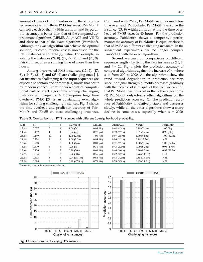
Among these tested PMS instances, (15, 5), (17, 6), (19, 7), (21, 8) and (23, 9) are challenging ones [1]. An instance is challenging if the input sequences are expected to contain one or more (l, d) motifs that occur by random chance. From the viewpoint of computa-tional cost of exact algorithms, solving challenging instances with large l (l > 15) requires huge time overhead. PMS5 [27] is an outstanding exact algo-rithm for solving challenging instances. Fig. 3 shows the time overhead and prediction accuracy of Pair-Motif+ and PMS5 on these challenging instances.

Compared with PMS5, PairMotif+ requires much less time overhead. Particularly, PairMotif+ can solve the instance (23, 9) within an hour, while the time over-head of PMS5 exceeds 40 hours. For the prediction accuracy, PairMotif+ shows a competitive perfor-mance: the accuracy of PairMotif+ is equal or close to that of PMS5 on different challenging instances. In the subsequent experiments, we no longer compare PairMotif+ with the exact algorithms.

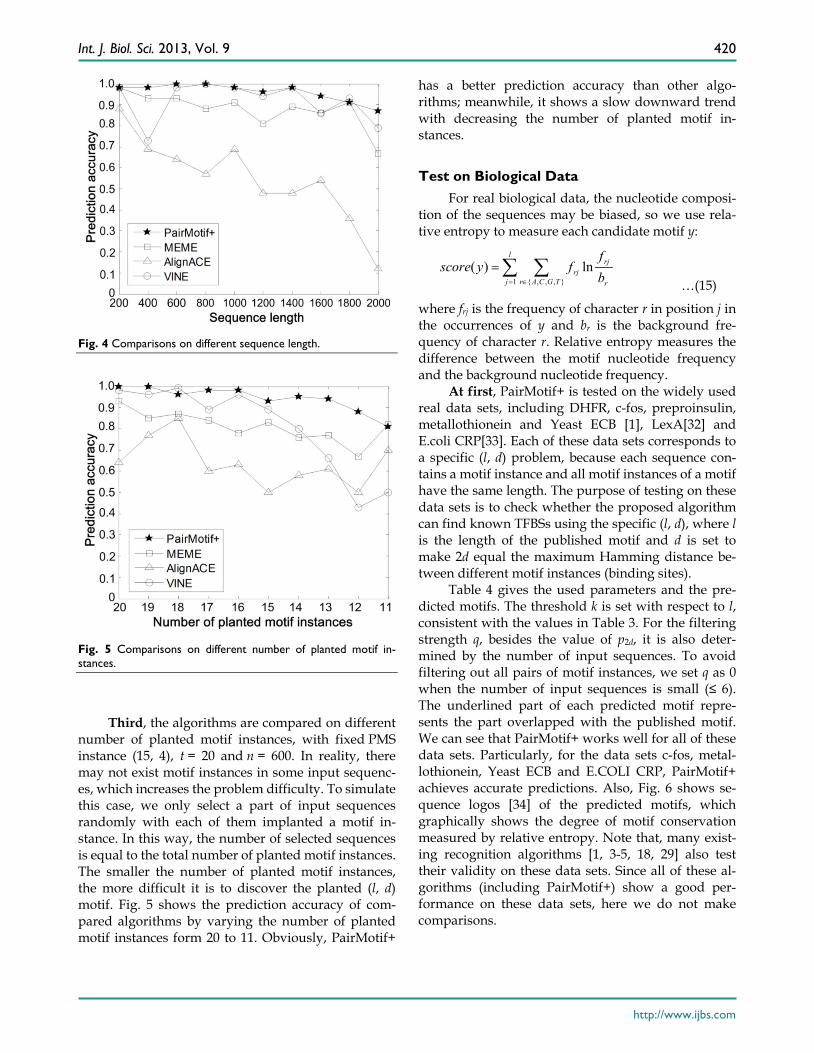
Second, we carry out comparisons on different sequence length n by fixing the PMS instance as (15, 4) and t = 20. Fig. 4 plots the prediction accuracy of compared algorithms against the increase of n, where n is from 200 to 2000. All the algorithms show the trend toward degradation in prediction accuracy, since the signal strength of motifs decreases gradually with the increase of n. In spite of this fact, we can find that PairMotif+ performs better than other algorithms: (1) PairMotif+ outperforms other algorithms on the whole prediction accuracy; (2) The prediction accu-racy of PairMotif+ is relatively stable and decreases slowly, while all the other algorithms show a sharp decline in some cases, especially when n = 2000.

Table 3. Comparisons on PMS instances with different 2d-neighborhood probability.

(l, d) p2d k q PairMotif+ MEME AlignACE VINE PairMotif (15, 4) 0.057 5 4 1.00 (2s) 0.93 (6s) 0.64 (4.3m) 0.98 (7.1m) 1.00 (2s) (14, 4) 0.112 4 4 0.94 (2s) 0.77 (6s) 0.59 (2.7m) 0.91 (8.4m) 0.96 (14s) (25, 8) 0.149 10 4 1.00 (2.4m) 1.00 (6s) 0.97 (2.5m) 1.00 (9.6m) 1.00 (52.3m) (24, 8) 0.234 9 4 1.00 (3.0m) 0.98 (6s) 0.86 (2.2m) 0.98(12.2m) > 5h (18, 6) 0.283 6 3 1.00 (14s) 0.89 (6s) 0.51 (2.1m) 1.00 (9.3m) 1.00 (12.1m) (15, 5) 0.319 5 3 0.95 (3s) 0.76 (6s) 0.43 (2.2m) 0.70 (8.7m) 0.95 (4.7m) (17, 6) 0.426 6 3 0.90 (26s) 0.66 (6s) 0.40 (3.6m) 0.80 (9.5m) 0.93 (53.3m) (19, 7) 0.534 7 3 0.96 (58s) 0.56 (6s) 0.42 (3.2m) 0.76 (10.1m) > 5h (21, 8) 0.633 8 3 0.94 (18.1m) 0.68 (6s) 0.48 (3.2m) 0.88 (13.4m) > 5h (23, 9) 0.698 9 3 0.98 (47.9m) 0.76 (6s) 0.53 (3.5m) 0.85 (15.2m) > 5h Time units, s: seconds; m: minutes; h: hours.

Fig. 3 Comparisons on challenging PMS instances.


http://www.ijbs.com

420

Fig. 4 Comparisons on different sequence length.

Fig. 5 Comparisons on different number of planted motif in-stances.

Third, the algorithms are compared on different

number of planted motif instances, with fixed PMS instance (15, 4), t = 20 and n = 600. In reality, there may not exist motif instances in some input sequenc-es, which increases the problem difficulty. To simulate this case, we only select a part of input sequences randomly with each of them implanted a motif in-stance. In this way, the number of selected sequences is equal to the total number of planted motif instances. The smaller the number of planted motif instances, the more difficult it is to discover the planted (l, d) motif. Fig. 5 shows the prediction accuracy of com-pared algorithms by varying the number of planted motif instances form 20 to 11. Obviously, PairMotif+

has a better prediction accuracy than other algo-rithms; meanwhile, it shows a slow downward trend with decreasing the number of planted motif in-stances.

Test on Biological Data For real biological data, the nucleotide composi-

tion of the sequences may be biased, so we use rela-tive entropy to measure each candidate motif y:

…(15)

where frj is the frequency of character r in position j in the occurrences of y and br is the background fre-quency of character r. Relative entropy measures the difference between the motif nucleotide frequency and the background nucleotide frequency.

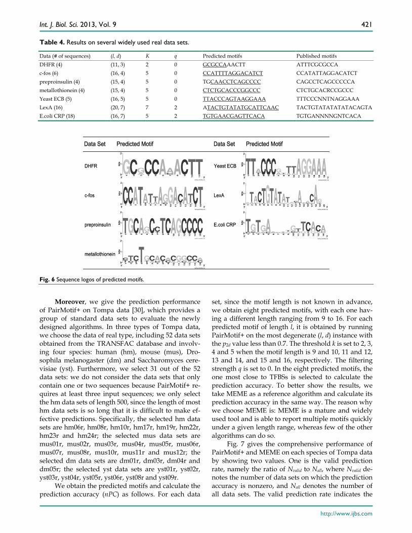
At first, PairMotif+ is tested on the widely used real data sets, including DHFR, c-fos, preproinsulin, metallothionein and Yeast ECB [1], LexA[32] and E.coli CRP[33]. Each of these data sets corresponds to a specific (l, d) problem, because each sequence con-tains a motif instance and all motif instances of a motif have the same length. The purpose of testing on these data sets is to check whether the proposed algorithm can find known TFBSs using the specific (l, d), where l is the length of the published motif and d is set to make 2d equal the maximum Hamming distance be-tween different motif instances (binding sites).

Table 4 gives the used parameters and the pre-dicted motifs. The threshold k is set with respect to l, consistent with the values in Table 3. For the filtering strength q, besides the value of p2d, it is also deter-mined by the number of input sequences. To avoid filtering out all pairs of motif instances, we set q as 0 when the number of input sequences is small (≤ 6). The underlined part of each predicted motif repre-sents the part overlapped with the published motif. We can see that PairMotif+ works well for all of these data sets. Particularly, for the data sets c-fos, metal-lothionein, Yeast ECB and E.COLI CRP, PairMotif+ achieves accurate predictions. Also, Fig. 6 shows se-quence logos [34] of the predicted motifs, which graphically shows the degree of motif conservation measured by relative entropy. Note that, many exist-ing recognition algorithms [1, 3-5, 18, 29] also test their validity on these data sets. Since all of these al-gorithms (including PairMotif+) show a good per-formance on these data sets, here we do not make comparisons.

∑ ∑= ∈

=l

j TGCAr r

rjrj b

ffyscore

1 },,,{

ln)(


http://www.ijbs.com

421

Table 4. Results on several widely used real data sets.

Data (# of sequences) (l, d) K q Predicted motifs Published motifs DHFR (4) (11, 3) 2 0 GCGCCAAACTT ATTTCGCGCCA c-fos (6) (16, 4) 5 0 CCATTTTAGGACATCT CCATATTAGGACATCT preproinsulin (4) (15, 4) 5 0 TGCAACCTCAGCCCC CAGCCTCAGCCCCCA metallothionein (4) (15, 4) 5 0 CTCTGCACCCGGCCC CTCTGCACRCCGCCC Yeast ECB (5) (16, 5) 5 0 TTACCCAGTAAGGAAA TTTCCCNNTNAGGAAA LexA (16) (20, 7) 7 2 ATACTGTATATGCATTCAAC TACTGTATATATATACAGTA E.coli CRP (18) (16, 7) 5 2 TGTGAACGAGTTCACA TGTGANNNNGNTCACA

Fig. 6 Sequence logos of predicted motifs.

Moreover, we give the prediction performance

of PairMotif+ on Tompa data [30], which provides a group of standard data sets to evaluate the newly designed algorithms. In three types of Tompa data, we choose the data of real type, including 52 data sets obtained from the TRANSFAC database and involv-ing four species: human (hm), mouse (mus), Dro-sophila melanogaster (dm) and Saccharomyces cere-visiae (yst). Furthermore, we select 31 out of the 52 data sets: we do not consider the data sets that only contain one or two sequences because PairMotif+ re-quires at least three input sequences; we only select the hm data sets of length 500, since the length of most hm data sets is so long that it is difficult to make ef-fective predictions. Specifically, the selected hm data sets are hm06r, hm08r, hm10r, hm17r, hm19r, hm22r, hm23r and hm24r; the selected mus data sets are mus01r, mus02r, mus03r, mus04r, mus05r, mus06r, mus07r, mus08r, mus10r, mus11r and mus12r; the selected dm data sets are dm01r, dm03r, dm04r and dm05r; the selected yst data sets are yst01r, yst02r, yst03r, yst04r, yst05r, yst06r, yst08r and yst09r.

We obtain the predicted motifs and calculate the prediction accuracy (nPC) as follows. For each data

set, since the motif length is not known in advance, we obtain eight predicted motifs, with each one hav-ing a different length ranging from 9 to 16. For each predicted motif of length l, it is obtained by running PairMotif+ on the most degenerate (l, d) instance with the p2d value less than 0.7. The threshold k is set to 2, 3, 4 and 5 when the motif length is 9 and 10, 11 and 12, 13 and 14, and 15 and 16, respectively. The filtering strength q is set to 0. In the eight predicted motifs, the one most close to TFBSs is selected to calculate the prediction accuracy. To better show the results, we take MEME as a reference algorithm and calculate its prediction accuracy in the same way. The reason why we choose MEME is: MEME is a mature and widely used tool and is able to report multiple motifs quickly under a given length range, whereas few of the other algorithms can do so.

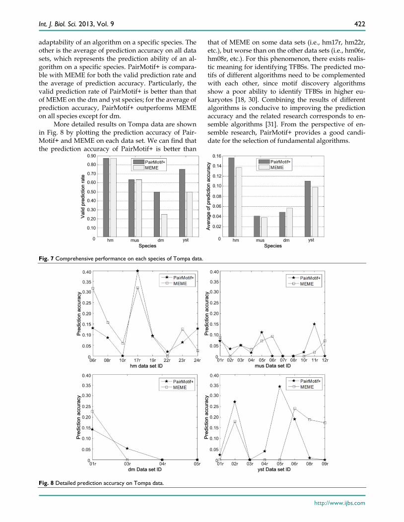
Fig. 7 gives the comprehensive performance of PairMotif+ and MEME on each species of Tompa data by showing two values. One is the valid prediction rate, namely the ratio of Nvalid to Nall, where Nvalid de-notes the number of data sets on which the prediction accuracy is nonzero, and Nall denotes the number of all data sets. The valid prediction rate indicates the


http://www.ijbs.com

422

adaptability of an algorithm on a specific species. The other is the average of prediction accuracy on all data sets, which represents the prediction ability of an al-gorithm on a specific species. PairMotif+ is compara-ble with MEME for both the valid prediction rate and the average of prediction accuracy. Particularly, the valid prediction rate of PairMotif+ is better than that of MEME on the dm and yst species; for the average of prediction accuracy, PairMotif+ outperforms MEME on all species except for dm.

More detailed results on Tompa data are shown in Fig. 8 by plotting the prediction accuracy of Pair-Motif+ and MEME on each data set. We can find that the prediction accuracy of PairMotif+ is better than

that of MEME on some data sets (i.e., hm17r, hm22r, etc.), but worse than on the other data sets (i.e., hm06r, hm08r, etc.). For this phenomenon, there exists realis-tic meaning for identifying TFBSs. The predicted mo-tifs of different algorithms need to be complemented with each other, since motif discovery algorithms show a poor ability to identify TFBSs in higher eu-karyotes [18, 30]. Combining the results of different algorithms is conducive to improving the prediction accuracy and the related research corresponds to en-semble algorithms [31]. From the perspective of en-semble research, PairMotif+ provides a good candi-date for the selection of fundamental algorithms.

Fig. 7 Comprehensive performance on each species of Tompa data.

Fig. 8 Detailed prediction accuracy on Tompa data.


http://www.ijbs.com

423

Discussion and Conclusions Buhler and Tompa introduced a formal descrip-

tion of the motif search problem in 2002, the planted (l, d) motif search (PMS) [1]. In the next year, Evans et al. proved the NP-hardness of the PMS problem by analyzing the complexity of finding common ap-proximate substrings [2]. The initial version of PMS assumed that there are exactly d different positions between a motif and a motif instance. To more effec-tively predict motifs in real biological data, in recent years researches (including us) have begun to focus on an improved version where a motif instance differs from the associated motif in at most d positions.

Numerous algorithms, either exact or approxi-mate, have been proposed to identify (l, d) motifs. The principle of the exact algorithms is to report all (l, d) motifs and the optimal one using as little time as pos-sible. In our previous work, we proposed an exact algorithm named PairMotif [29]. PairMotif is able to quickly solve many PMS instances except for the challenging ones with large l, such as (21, 8) and (23, 9). To the best of our knowledge, PMS5 [27] is the fastest exact algorithm for solving challenging in-stances with large l, but its time overhead is still far from satisfactory. The aim of most approximate recognition algorithms is to get as good results as possible in a short time, such as MEME [6], which always returns results within several seconds. In solving some PMS instances, such as (15, 4) and (18, 6), MEME achieves a good prediction accuracy. However, MEME, as well as many other approximate algorithms, shows a poor ability to identify highly degenerate motifs.

In the present study, we aim to make a good trade-off between prediction accuracy and time per-formance for motif search. Specifically, our goal is to use a reasonable time (within an hour on personal computers) to obtain results with high accuracy. This goal is achieved by designing a new algorithm called PairMotif+ using the strategy of PairMotif: extract some pairs of l-mers from input sequences S, and then refine each of them. Unlike PairMotif, PairMotif+ completes these tasks using the method based on probabilistic analysis rather than the exhaustive search.

From the theoretical perspective, PairMotif+ guarantees both a good time performance (efficiency) and a good prediction accuracy (validity). To get good time performance, we extract pairs of l-mers from S with the restriction of the threshold k and further filter them using the filtering strength q. After these opera-tions, the number of pairs to be refined by PairMotif+ is about O(n), far less than the number of pairs pro-cessed by PariMotif, O(n2). Moreover, in refining pairs

of l-mers, unlike PairMotif that verifies all possible candidate motifs, PairMotif+ adopts an approximate refinement strategy and avoids the verification of most candidate motifs.

To achieve good prediction accuracy, first, the pairs of l-mers to be refined should contain at least one pair of motif instances, and the key point is to set the parameters k and q according to probabilistic analysis and statistical method; second, in refining pairs of l-mers, the generated candidate motifs should contain the desired motif, and the key point is to de-termine which part of subsets in the partition of can-didate motifs should be generated in terms of proba-bilistic analysis. The foundation required by all of these work is the distance relation between a motif m and its instance m'. The basic distance relation that m and m' differ by at most d positions is not specific enough to carry out probabilistic analysis. Therefore, based on the basic relation, we adopt a more specific version, namely the expectation of the distance be-tween m and m' is 3d/4, which allows us to quantita-tively analyze how to set appropriate parameters. The choice of this expectation is reasonable: if the expec-tation is too small, then our algorithm can only iden-tify the highly conserved motifs and lacks a good scalability; if the expectation is d, it is not consistent with the practical biological case and will also de-crease the time performance of our algorithm.

Experimental results also demonstrate the effi-ciency and validity of PairMotif+. From the results on simulated data, we can find: (1) PairMotif+ is able to solve various PMS instances within an hour on per-sonal computers. Particularly, all instances except for (21, 8) and (23, 9) are solved within several seconds to several minutes. (2) The prediction accuracy of Pair-Motif+ is better than that of the compared algorithms and close to the optimal solution. (3) PairMotif+ shows a stable prediction as the sequence length is increased. (4) It is easy to extend PairMotif+ to solve the motif search problem that is not in the case of OOPS (one motif occurrence per sequence), and the prediction accuracy is stable over different number of planted motif instances. Moreover, for the experi-ments on real biological data, we use two groups of data sets: (1) The first group includes DHFR, c-fos, preproinsulin, metallothionein and Yeast ECB [1], LexA[32] and E.coli CRP[33], which are used by many existing recognition algorithms to test their validity. For each of these data sets, PairMotif+ is able to find all or a large part of TFBSs. (2) The second group of data sets is the Tompa data [30], the standard data sets to evaluate the newly designed recognition algo-rithms. The comprehensive performance of PairMo-tif+ is comparable with that of the mature and popu-lar algorithm MEME.


http://www.ijbs.com

424

In summary, we have proposed a new approxi-mate algorithm for the PMS problem and tested it on both simulated data and real biological data. This algorithm is good at identifying highly degenerate motifs, and outperforms the compared algorithms in identification accuracy. Although the execution time increases with the increase of the motif length, which is determined by the used pattern-driven framework, the proposed algorithm is able to solve various PMS instances within an hour on personal computers.

Acknowledgments This work was supported by the National Nat-

ural Science Foundation of China (61173025), the Re-search Fund for the Doctoral Program of Higher Ed-ucation of China (20100203110010), and the Funda-mental Research Funds for the Central Universities (K50513100011 and K5051303002).

Conflict of Interest All authors have declared that no conflicts of in-

terest exist and agree with the contents of the manu-script for publication.

References 1. Buhler J, Tompa M. Finding motifs using random projections. J Comput

Biol. 2002; 9: 225-42. 2. Evans PA, Smith AD, Wareham HT. On the complexity of finding

common approximate substrings. Theor Comput Sci. 2003; 306: 407-30. 3. Ho ES, Jakubowski CD, Gunderson SI. iTriplet, a rule-based nucleic acid

sequence motif finder. Algorithm Mol Biol. 2009; 4: 14. 4. Sun HQ, Low MYH, Hsu WJ, et al. RecMotif: a novel fast algorithm for

weak motif discovery. BMC Bioinformatics. 2010; 11(Suppl 11): S8. 5. Davila J, Balla S, Rajasekaran S. Fast and practical algorithms for planted

(l, d) motif search. IEEE ACM T Comput Bi. 2007; 4: 544-52. 6. Bailey TL, Williams N, Misleh C, et al. MEME: discovering and analyz-

ing DNA and protein sequence motifs. Nucleic Acids Res. 2006; 34: 369-73.

7. Lawrence CE, Altschul SF, Boguski MS, et al. Detecting subtle sequence signals: a Gibbs sampling strategy for multiple alignment. Science. 1993; 262: 208-14.

8. Li L. GADEM: a genetic algorithm guided formation of spaced dyads coupled with an EM algorithm for motif discovery. J Comput Biol. 2009; 16: 317-29.

9. Neuwald AF, Liu JS, Lawrence CE. Gibbs motif sampling: detection of bacterial outer membrane protein repeats. Protein Sci. 1995; 4: 1618-32.

10. Hughes JD, Estep PW, Tavazoie S, et al. Computational identification of Cis-regulatory elements associated with groups of functionally related genes in Saccharomyces cerevisiae. J Mol Biol. 2000; 296: 1205-14.

11. Thijs G, Lescot M, Marchal K, et al. A higher-order background model improves the detection of promoter regulatory elements by Gibbs sam-pling. Bioinformatics. 2001; 17: 1113-22.

12. Tang ME, Krogh A, Winther O. BayesMD: flexible biological modeling for motif discovery. J Comput Biol. 2008; 15: 1347-63.

13. Kim N, Tharakaraman K, Mariño-Ramírez L, et al. Finding sequence motifs with Bayesian models incorporating positional information: an application to transcription factor binding sites. BMC Bioinformatics. 2008; 9: 262.

14. Miller AK, Print CG, Nielsen PMF, et al. A Bayesian search for tran-scriptional motifs. PLoS One. 2010; 5: e13897.

15. Jajamovich GH, Wang XD, Arkin AP, et al. Bayesian multiple-instance motif discovery with BAMBI: inference of recombinase and transcription factor binding sites. Nucleic Acids Res. 2011; 39: e146.

16. Fratkin E, Naughton BT, Brutlag DL, et al. MotifCut: regulatory motifs finding with maximum density subgraphs. Bioinformatics. 2006; 22: e150-7.

17. Boucher C, King J. Fast motif recognition via application of statistical thresholds. BMC Bioinformatics. 2010; 11(Suppl 1): S11.

18. Huang CW, Lee WS, Hsieh SY. An improved heuristic algorithm for finding motif signals in DNA sequences. IEEE ACM T Comput Bi. 2011; 8: 959-75.

19. Jones NC, Pevzner PA. An introduction to bioinformatics algorithms. Cambridge: MIT Press; 2004.

20. Yang X, Rajapakse JC. Graphical approach to weak motif recognition. Genome Inform. 2004; 15: 52-62.

21. Vanet A, Marsan L, Labigne A, et al. Inferring regulatory elements from a whole genome: an analysis of helicobacter pylori σ80 family of promoter signals. J Mol Biol. 2000; 297: 335-53.

22. Marsan L, Sagot M. Algorithms for extracting structured motifs using a suffix tree with an application to promoter and regulatory site consensus identification. J Comput Biol. 2000; 7: 345-62.

23. Pavesi G, Mauri G, Pesole G. An algorithm for finding signals of un-known length in DNA sequences. Bioinformatics. 2001; 17: 207-14.

24. Eskin E, Pevzner PA. Finding composite regulatory patterns in DNA sequences. Bioinformatics. 2002; 18: 354-63.

25. Rajasekaran S, Balla S, Huang CH. Exact algorithms for planted motif problems. J Comput Biol. 2005; 12: 1117-28.

26. Rajasekaran S, Balla S, Huang CH, et al. High-Performance exact algo-rithms for motif search. J Clin Monit Comput. 2005; 19: 319-28.

27. Dinh H, Rajasekaran S, Kundeti VK. PMS5: an efficient exact algorithm for the (l, d)-motif finding problem. BMC Bioinformatics. 2011; 12: 410.

28. Dinh H, Rajasekaran S, Davila J. qPMS7: a fast algorithm for finding (l, d)-motifs in DNA and protein sequences. PLoS One. 2012; 7: e41425.

29. Yu Q, Huo HW, Zhang YP, et al. PairMotif: a new pattern-driven algo-rithm for planted (l, d) DNA motif search. PLoS One. 2012; 7: e48442.

30. Tompa M, Li N, Bailey TL, et al. Assessing computational tools for the discovery of transcription factor binding sites. Nat Biotechnol. 2005; 23: 137-44.

31. Hu J, Li B, Kihara D. Limitations and potentials of current motif discov-ery algorithms. Nucleic Acids Res. 2005; 33: 4899-913.

32. Hertz GZ, Hartzell GW. Identification of consensus patterns in una-ligned DNA sequences known to be functionally related. Comput Appl Biosci. 1990; 6: 81-92.

33. Stormo GD, Hartzell GW. Identifying protein-binding sites from una-ligned DNA fragments. Proc Natl Acad Sci USA. 1989; 86: 1183-7.

34. Crooks GE, Hon G, Chandonia JM, et al. WebLogo: a sequence Logo generator. Genome Res. 2004; 14: 1188-90.

Documents

PairMotif+: A Fast and Effective Algorithm for De Novo Motif Discovery in DNA sequences