Embed Size (px)
Citation preview
© 2017 Pakistan Journal of Statistics 135
Pak. J. Statist.
2017 Vol. 33(2), 135-160
PERFORMANCE OF SOME BIASED ESTIMATORS IN MISSPECIFIED
MODEL UNDER MAHALANOBIS LOSS FUNCTION
Gargi Tyagi§ and Shalini Chandra
Department of Mathematics & Statistics, Banasthali University
Rajasthan-304022, India.
Email: §[email protected]
ABSTRACT
In econometric research, misspecification due to omission of relevant variables is a
very common phenomena, which leads to biased and inconsistent estimation of
parameters. It is needless to mention that the explanatory variables in the misspecified
model may be multicollinear and have adverse effects on the least squares estimator. To
combat the problem of multicollinearity, several biased estimators have been introduced
and widely analyzed under mean squared error criterion when there is no
misspecification. Furthermore, Mahalanobis loss function, which is a weighted quadratic
loss function has gained quite an attention as a comparison criterion in recent years.
Although, not much literature is available on the comparison of the estimators in the
presence of multicollinearity under the Mahalanobis loss function when there is no
misspecification and is almost negligible in case of misspecification due to omission of
relevant variables. This article evaluates the performance of some biased estimators in the
presence of multicollinearity under the Mahalanobis loss function using average loss
criterion in the misspecified model. Necessary and sufficient conditions for the
dominance of one estimator over the others have been derived. Further, the findings are
supported by a Monte Carlo simulation and numerical example.
KEYWORDS
Omission of relevant variables, multicollinearity, biased estimators, Mahalanobis loss
function, average loss criterion.
1. INTRODUCTION
Multicollinearity among the regressors is a common problem in regression analysis,
its one of the major consequences is that it produces larger sampling variance of the
ordinary least squares (OLS) estimator and makes it unsteady. A solution to this problem
is found in making use of more consistent biased estimators such as, the ordinary ridge
regression (ORR) estimator, the principal component regression (PCR) estimator, the
class estimator, the Liu estimator, the class estimator and the two-parameter
class estimator, introduced by Hoerl and Kennard (1970), Massy (1965), Baye and Parker
(1984), Liu (1993), Kaçiranlar and Sakallioğlu (2001) and Özkale and Kaçiranlar (2007),
respectively. Recently, Özkale (2012) merged the approaches of the two-parameter class
estimator and the PCR estimator and put forward the class estimator.
Performance of some biased estimators in misspecified model… 136
In applied work misspecification may occur due to one reason or another. There are
mainly two reasons for misspecification, inclusion of superfluous variables or omission
of relevant variables. The misspecification in linear regression model has many
undesirable effects on the properties of the estimators (see Johnston DiNardo (1997)).
Several authors have studied the effect of misspecification on estimation of regression
coefficients, for instance, Kadiyala (1986); Sarkar (1989); Wijekoon and Trenkler (1989),
Dube et al. (1991), Groß et al. (1998), Dube (1999), Hubert and Wijekoon (2004),
Uemukai (2010), Jianwen and Hu (2012), Şiray (2015) and Wu (2016) among others.
The criterion of average loss under squared error loss function, famously known as
mean squared error (MSE) criterion is one of the most popular criterion to evaluate the
performance of the estimators. Baye and Parker (1984) revealed the MSE superiority of
the class estimator over the PCR estimator. Nomura and Ohkubo (1985) derived
the dominance conditions of the class estimator over the OLS and ORR estimators
under MSE criterion and Sarkar (1996) obtained conditions for the superiority of the
class estimator over the OLS, PCR and the ORR estimators by the MSE matrix
criterion. Özkale and Kaçiranlar (2007) have also compared the class estimator
with the PCR estimator, class estimator and Liu estimator by the MSE matrix
criterion. Sarkar (1989) compared the performances of the class estimator with the
OLS, ORR and PCR in misspecified linear regression model. Şiray (2015) made a
comparison between the performance of the class estimator with others when some
relevant variables get omitted. Jianwen and Hu (2012) compared the stochastic restricted
Liu estimator with others when there is inclusion of superfluous variables.
Furthermore, Peddada et al. (1989) pointed out that the Malahanobis loss function
(Mahalanobis (1936)), can be used to compare two estimators if at least one of them is
biased, and compared the generalized ridge estimator and the OLS estimator in a linear
regression model. Şiray et al. (2012) examined the performance of the class
estimator over the OLS, ORR and PCR estimators in terms of the Mahalanobis loss
function using average loss criterion, further referred as average Mahalanobis loss
criterion. Sarkar and Chandra (2015) obtained conditions of superiority of the
class estimator over the OLS, PCR and the two-parameter class estimators by means of
the average Mahalanobis loss criterion.
Sarkar (1989) discussed the effect of omission of relevant variables on the dominance
conditions of the class estimator over the other competing estimators. Şiray (2015)
studied the performance of the class estimator and others in case of omission of
relevant variables. Wu (2016) compared the class estimator with the OLS, ORR
and the PCR estimators under the average Mahalanobis loss criterion when there is
misspecification due to omission of relevant variables. Chandra and Tyagi (2017) studied
consequences of omission of relevant variables on the superiority conditions of the
class estimator over the others in mean squared error sense.
This paper discusses the effect of misspecification due to omission of relevant
variables on the performance of the class estimator with other competing
estimators such as the OLS, ORR, PCR, Liu estimator, class estimator, class
estimator and the two-parameter class estimator under the Mahalanobis loss function
using average loss criterion. The rest of the paper is designed in the following manner:
Tyagi and Chandra 137
Section 2 discusses the model and the estimators under consideration, comparison of the
estimators under the Mahalanobis loss has been done in Section 3 and the conditions of
dominance of several estimators over the other estimators have also been derived. The
estimators are compared by Monte Carlo simulation study in Section 4 and Section 5
illustrates theoretical findings with a numerical example. The paper is then concluded in
Section 6.
2. MODEL AND ESTIMATORS
Let us consider the classical linear regression model which is assumed to be a true
model
(2.1)
where is an vector of dependent variable, is an matrix of explanatory
variables of rank and is a matrix of some other relevant explanatory variables of rank
, , and are the corresponding and vectors of parameters
associated with and , respectively. is an vector of disturbance term and
assume that .
In regression analysis, omission of relevant variables is a very common problem. It
increases the bias in the estimator and also affects the validity of conventional inference
procedures. Now, suppose that investigator has unknowingly excluded variables of
matrix, thus the misspecified model is given by
(2.2)
where, . Misspecification occurs when investigator assumes the disturbance
vector to be normally distributed with mean vector and variance .
In order to define the estimators, let us assume that is an
orthogonal matrix of order with is a
diagonal matrix of eigen values of matrix such that . Now, let
be orthogonal matrix after deleting last columns from
matrix, where . Thus, where and
, . Also, .
Özkale (2012) introduced an estimator known as ) class estimator to deal
with multicollinearity. This estimator for the misspecified model in (2.2) can be written
as
(2.3)
This is a general class of estimators which includes the OLS, ORR, Liu, PCR,
class estimator, class estimator and the two-parameter class estimator as its special
cases.
(i) , is the OLS estimator,
(ii) , is the ORR estimator,
(iii)
, is the PCR estimator,
Performance of some biased estimators in misspecified model… 138
(iv) , is the Liu estimator.
(v)
, is the class estimator,
(vi)
, is the class
estimator.
(vii) , is the two-parameter class
estimator.
After some straightforward calculations, expectation and covariance of the
class estimator in misspecified model can be obtained as
Further,
(2.4)
where and .
3. AVERAGE LOSS COMPARISONS UNDER MAHALANOBIS LOSS
For an estimator of Mahalanobis loss function is defined as
The above form of the loss function can not be applied for the estimators such as the
PCR, class estimator, class estimator and the class estimator as
the covariance matrix for these estimators is singular. So, a more general form of the loss
function can be given as
where ’+’ denotes Moore-Penrose inverse of the matrix.
Therefore, Mahalanobis loss function for the ) class estimator in
misspecified model can be written as
(3.1)
The Moore-Penrose inverse of covariance matrix in (2.4) is given as
( ( ))
On substituting the expressions for from (2.3) and ( (
))
in (3.1), and on further simplification, we get
Further, risk under the Mahalanobis loss function or average Mahalanobis loss can be
obtained as follows
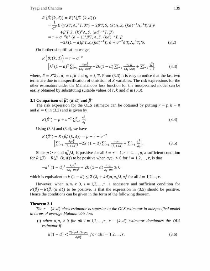
Tyagi and Chandra 139
. (3.2)
On further simplification,we get
( )
* ∑
∑
∑
+ (3.3)
where, , and . From (3.3) it is easy to notice that the last two
terms are due to misspecification of omission of variables. The risk expressions for the
other estimators under the Mahalanobis loss function for the misspecified model can be
easily obtained by substituting suitable values of and in (3.3).
3.1 Comparison of and
The risk expression for the OLS estimator can be obtained by putting
and in (3.3) and is given by
∑
(3.4)
Using (3.3) and (3.4), we have
*∑
∑
∑
+ (3.5)
Since and is positive for all , a sufficient condition
for to be positive when for , is that
which is equivalent to for all .
However, when , , a necessary and sufficient condition for
to be positive, is that the expression in (3.5) should be positive.
Hence the conditions can be given in the form of the following theorem.
Theorem 3.1
The class estimator is superior to the OLS estimator in misspecified model
in terms of average Mahalanobis loss
(i) when for all , estimator dominates the OLS
estimator if
(3.6)
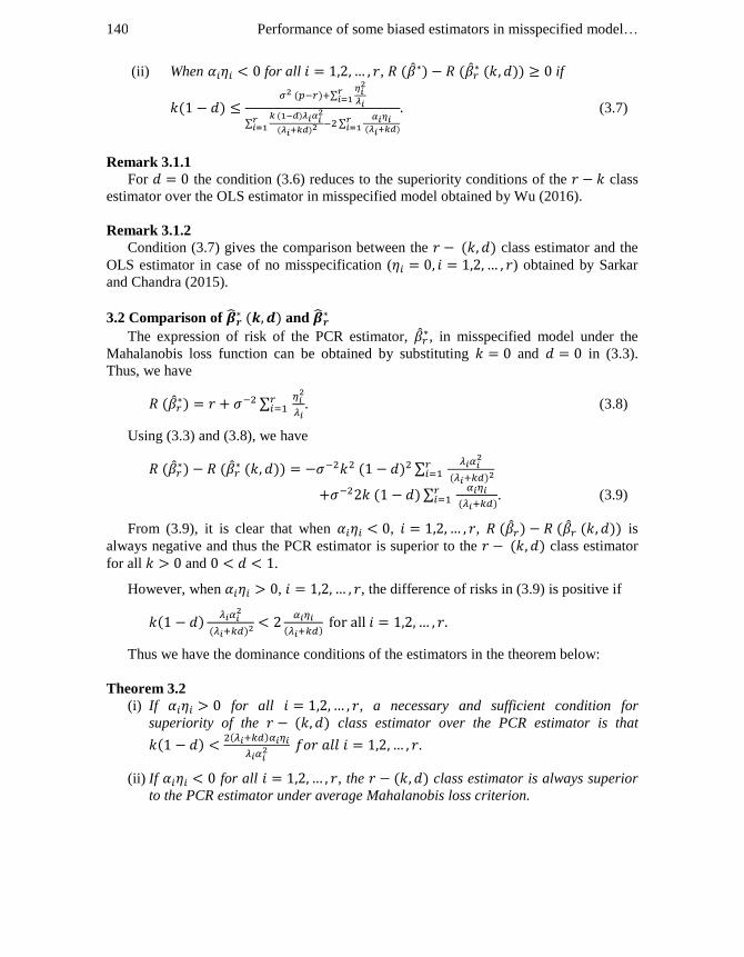
Performance of some biased estimators in misspecified model… 140
(ii) When for all , if
∑
∑
∑
(3.7)
Remark 3.1.1
For the condition (3.6) reduces to the superiority conditions of the class
estimator over the OLS estimator in misspecified model obtained by Wu (2016).
Remark 3.1.2
Condition (3.7) gives the comparison between the class estimator and the
OLS estimator in case of no misspecification ( ) obtained by Sarkar
and Chandra (2015).
3.2 Comparison of and
The expression of risk of the PCR estimator, , in misspecified model under the
Mahalanobis loss function can be obtained by substituting and in (3.3).
Thus, we have
∑
. (3.8)
Using (3.3) and (3.8), we have
∑
∑
. (3.9)
From (3.9), it is clear that when , , is
always negative and thus the PCR estimator is superior to the class estimator
for all and .
However, when , , the difference of risks in (3.9) is positive if
Thus we have the dominance conditions of the estimators in the theorem below:
Theorem 3.2
(i) If for all , a necessary and sufficient condition for
superiority of the class estimator over the PCR estimator is that
.
(ii) If for all , the class estimator is always superior
to the PCR estimator under average Mahalanobis loss criterion.
Tyagi and Chandra 141
Remark 3.2.1
For , the condition reduces to comparison between the class estimator and
the PCR in misspecified model obtained by Wu (2016).
Remark 3.2.2
It may be noted that in case of no misspecification Sarkar and Chandra (2015) showed
that the class estimator is always superior to the PCR estimator, however in the
misspecified model there may be some situations where the class estimator
dominates the PCR estimator.
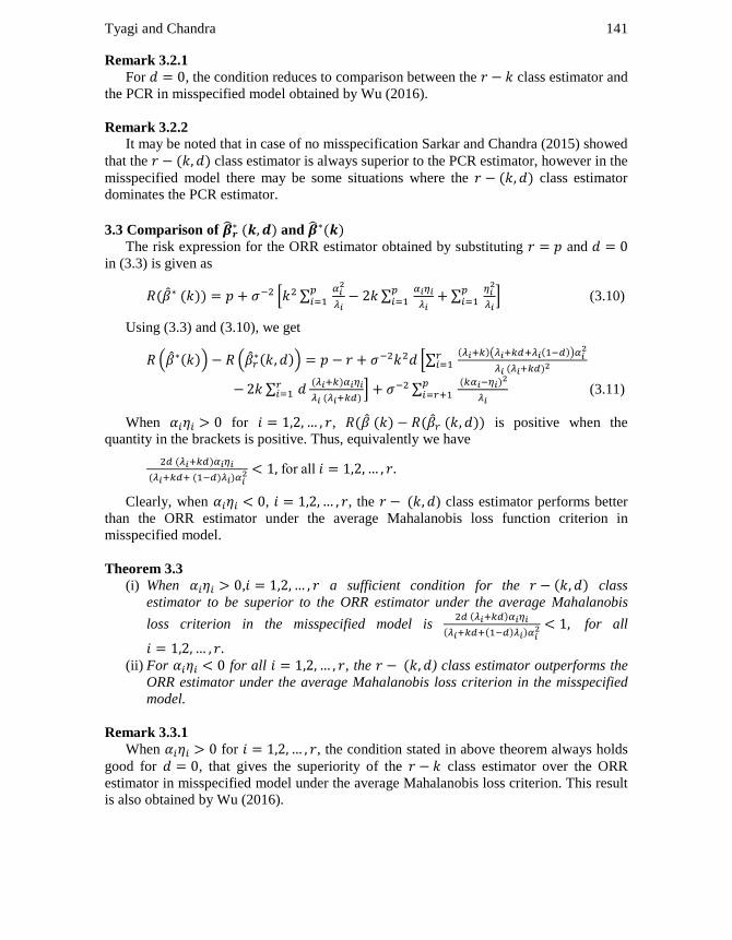
3.3 Comparison of and
The risk expression for the ORR estimator obtained by substituting and
in (3.3) is given as
* ∑
∑
∑
+ (3.10)
Using (3.3) and (3.10), we get
( ) ( ) *∑
( )
∑
+ ∑
(3.11)
When for , is positive when the
quantity in the brackets is positive. Thus, equivalently we have
o all
Clearly, when , , the ) class estimator performs better
than the ORR estimator under the average Mahalanobis loss function criterion in
misspecified model.
Theorem 3.3
(i) When , a sufficient condition for the class
estimator to be superior to the ORR estimator under the average Mahalanobis
loss criterion in the misspecified model is
for all
(ii) For for all , the ) class estimator outperforms the
ORR estimator under the average Mahalanobis loss criterion in the misspecified
model.
Remark 3.3.1
When for , the condition stated in above theorem always holds
good for , that gives the superiority of the class estimator over the ORR
estimator in misspecified model under the average Mahalanobis loss criterion. This result
is also obtained by Wu (2016).
Performance of some biased estimators in misspecified model… 142
Remark 3.3.2
It is evident from (3.11) that, in case of no misspecification (i.e.
the class estimator is always superior to the ORR estimator.
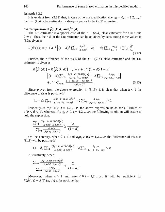
3.4 Comparison of and
The Liu estimator is a special case of the ) class estimator for and
. Thus, the risk of the Liu estimator can be obtained by substituting these values in
(3.3), given as
* ∑
∑
∑
+.
(3.12)
Further, the difference of the risks of the class estimator and the Liu
estimator is given as
( ) ( )
* ∑
(
)
∑
+
∑
. (3.13)
Since , from the above expression in (3.13), it is clear that when the
difference of risks is positive if
∑
∑
Evidently, if , , the above expression holds for all values of
), whereas, if , , the following condition will assure to
hold the expression.
∑
∑
On the contrary, when and the difference of risks in
(3.13) will be positive if
∑
∑
Alternatively, when
∑
∑
Moreover, when and , it will be sufficient for
to be positive that
Tyagi and Chandra 143
* ∑
∑
+
Thus, the dominance conditions can be stated as given in the following theorem.
Theorem 3.4
The sufficient conditions for class estimator to be superior to the Liu
estimator under the average Mahalanobis loss criterion are:
(i) When for all
a) and ∑
∑
.
b) and ∑
∑
.
(ii) When for all and
a) and
∑
*
+
b) and .
Remark 3.4.1
On substitution of in expression (3.13), we obtain a straightforward superiority
of the class estimator over the Liu estimator in misspecified model under the
average Mahalanobis loss criterion.
Remark 3.4.2
When there is no omission of relevant variables, that is ( , the
expression in (3.13) suggests that the class estimator performs better than the
class estimator for all values of , however for the range where the
) class estimator dominates the r-d class estimator may be obtained from
condition (ii) (a) in Theorem 3.4, as
∑
*
+.
3.5 Comparison of and
Risk under the Mahalanobis loss function of the two-parameter class estimator can be
obtained by substituting in (3.3). The expression can be written as
* ∑
∑
∑
+ (3.14)
Further, we have
* ∑
∑
∑
+
∑
(3.15)
Performance of some biased estimators in misspecified model… 144
From the above expression, it is clear that the class estimator always
dominates the two-parameter class estimator in misspecified model.
Theorem 3.5
The ) class estimator dominates the two-parameter class estimator under
the average Mahalanobis loss criterionin the misspecified model.
Remark 3.5.1
When for all , that is when there is no misspecification due to
omission, the result is same as obtained by Sarkar and Chandra (2015) when there is no
misspecification.
Remark 3.5.2
For , it gives us the comparison between the class estimator and the ORR
estimator which was obtained by Wu (2016).
Remark 3.5.3
For it gives the comparison of the class estimator with the Liu estimator
and for it compares the PCR and the OLS estimators under average Mahalanobis
loss criterionin misspecified model.
3.6 Comparison of and
Risk expression for the class estimator for misspecified model can be obtained
by substituting in (3.3), given as
* ∑
∑
∑
+. (3.16)
Further, we have
*∑
∑
+. (3.17)
From the above expression, the conditions of superiority of the class
estimator over the class estimator are very straightforward. When ,
, the right hand side of (3.17) is always positive and so is the difference of
risks. However, when , , the class estimator will
dominate the class estimator if
holds.
Hence, we have the conditions of dominance stated in the form of the following
theorem.

Tyagi and Chandra 145
Theorem 3.6
(i) When , , a necessary and sufficient condition for the
superiority of the class estimator over the class estimator under
the average Mahalanobis loss criterionin the misspecified model is
(ii) When , the class estimator is superior to the
class estimator under the average Mahalanobis loss criterion in the
misspecified model for all values of and .
Remark 3.6.1
When , that is in case of no misspecification the condition in the above theorem
always holds. Hence the class estimator always performs better than the
class estimator in the model with no misspecification under the Mahalanobis loss
function using average loss criterion.
3.7 Superiority of the ) Class Estimator Over the Class Estimator
The class estimator is a special case of the ) class estimator for .
Thus, the risk of the class estimator can be obtained by substituting these values in
(3.3), given as
* ∑
∑
∑
+
(3.18)
Further, from (3.3) and (3.18), we have
* ∑
∑
+ (3.19)
Following the steps similar to the comparison of the class estimator with
the Liu estimator in section 3.4, the conditions for superiority of the class
estimator over the class estimator can be given in the following theorem.
Theorem 3.7
i) When for all , the necessary and sufficient conditions for
superiority of the ) class estimator over the class estimator in the
misspecified model under the average Mahalanobis loss criterion are
a) , for all and ∑
∑
.
b) and ∑
∑
.
ii) When for all ,
a) for , the class estimator dominates the class estimator
for all values of .
Performance of some biased estimators in misspecified model… 146
b) For , the class estimator dominates the class estimator
in misspecified model under the average Mahalanobis loss criterion.
Remark 3.7.1
When there is no ommission of relevant variables in the model (When for
all ), the class estimator performs better than the class
estimator for , and for the class estimator outperforms the
class estimator under the average Mahalanobis loss critetion.
Now, we further examine the performance of the estimators in misspecified model
under the average Mahalanobis loss criterion by performing a simulation study.
4. MONTE CARLO SIMULATION
In this section a simulation study has been carried out to illustrate theoretical results
obtained in previous section. To compare the dominance of the estimators in misspecified
model, we take , and design matrix and have been generated by the
method given in [McDonald Galarneau (1975)] and [Gibbons (1981)], that is
where and are independent standard normal pseudo-random numbers and gives
the correlation between any two explanatory variables. The dependent variable has
been generated as follows:
(4.1)
matrix has been standardized such that forms correlation matrix of explanatory
variables. is a vector of normal pseudo random numbers with standard deviation .
and vectors have been taken such that and . The estimator of for
misspecified model has been estimated using and only and information on Z has not
been considered (i.e., are omitted from the model).
The simulation has been conducted for 50, 0.50,0.70,0.80,0.90,0.95,0.99,
0.1,1,10, 0.01,0.1,0.3,0.5,0.7,0.9,2 and 0.1,0.3,0.5,0.7,0.9,0.99. The value
of has been taken as the number of eigen values of matrix greater than 1, here it is
obtained to be . For each parametric combination, the simulation process has been
repeated 2000 times and average Mahalanobis loss is calculated by the following formula
∑
(4.2)
where is an estimator of in iteration.
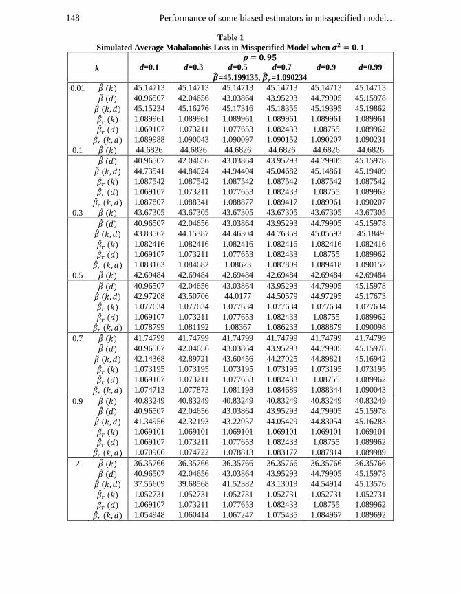
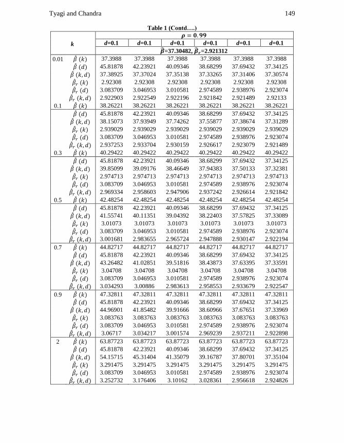
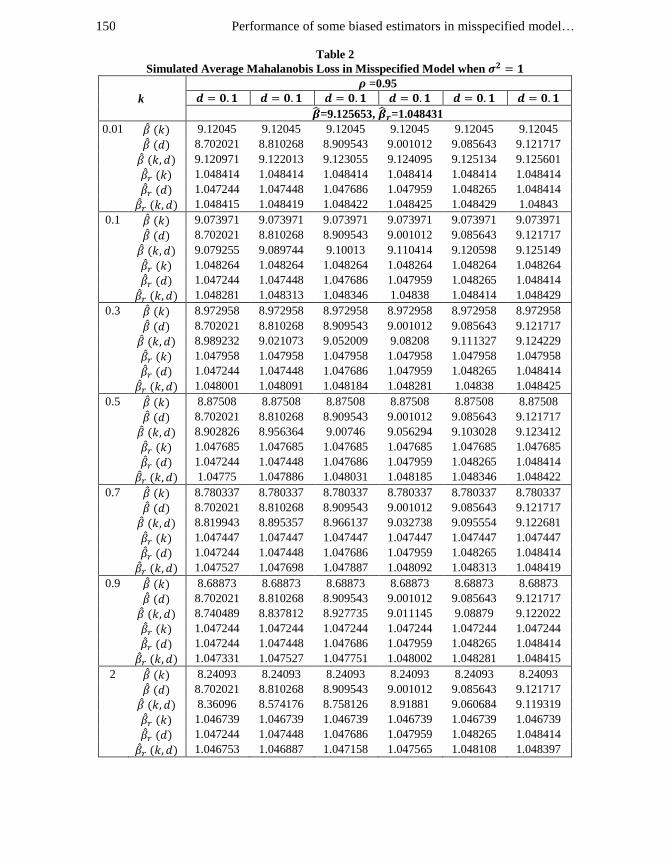
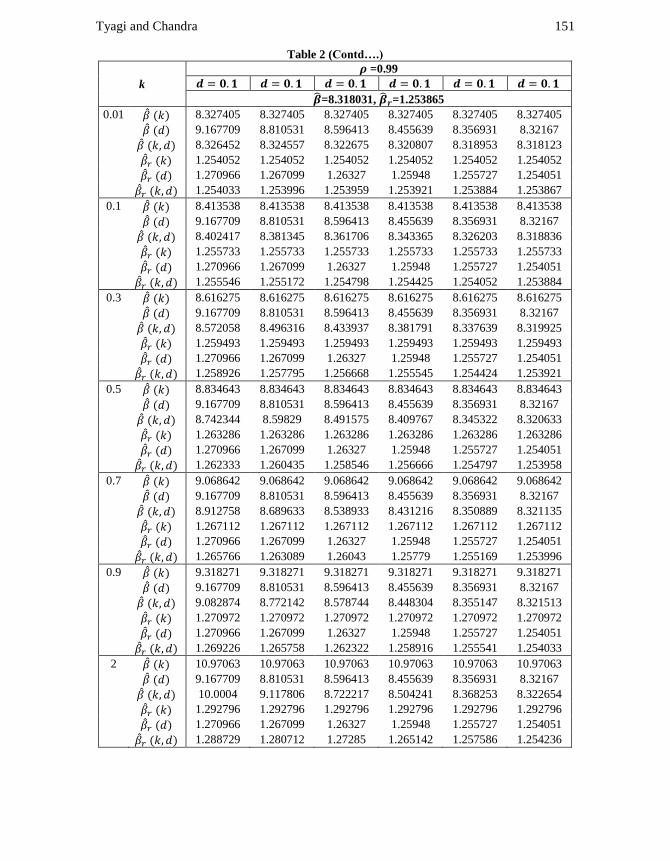
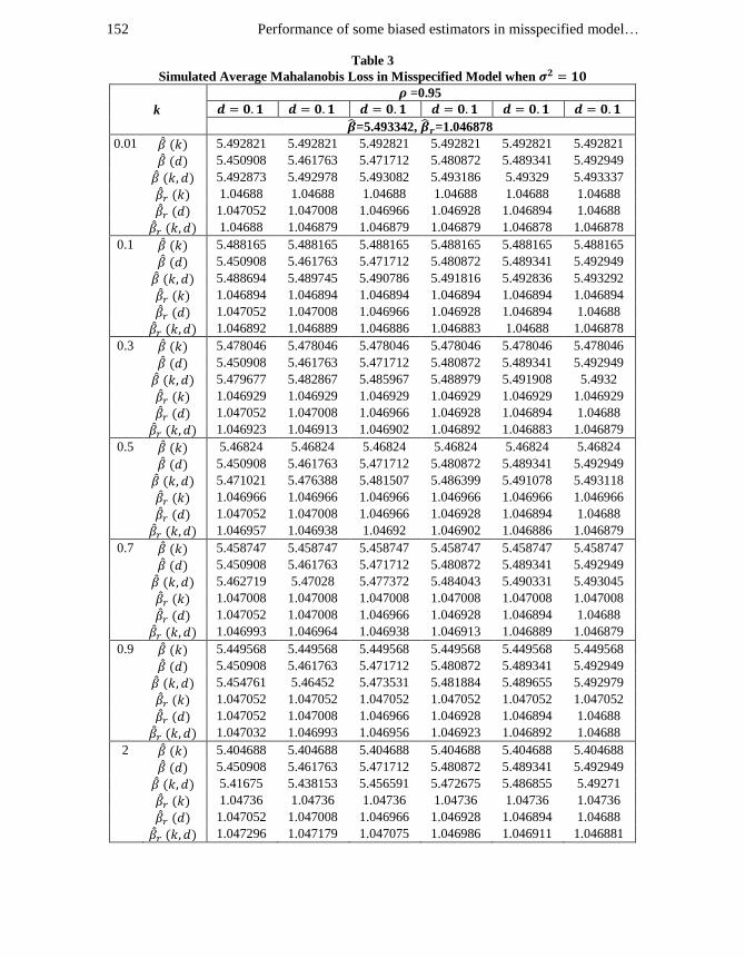
The simulation results are summarized in Tables 1-4. The following observations
were made:
The average Mahalanobis loss decreases as the value of increases, and it increases
as the value of increases for the values considered in this study. As it is evident from
the expression of average Mahalanobis loss, it decreases with the increase in the value of
Tyagi and Chandra 147
. From Tables 1-3, we see that when , the class estimator performs
better than all the other estimators except the and class estimators for ,
however for , only class estimator has lesser average loss than the
class estimator. When , for the class estimator is superior to
all the estimators except the PCR estimator, nevertheless the PCR and class
estimators perform better than the class estimator for .
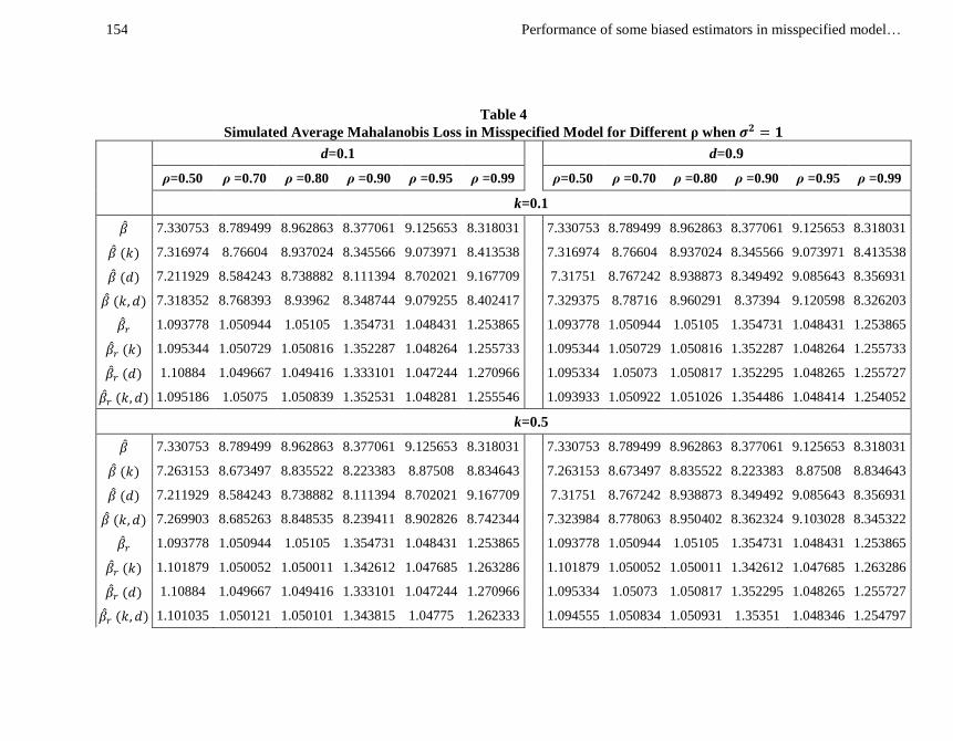
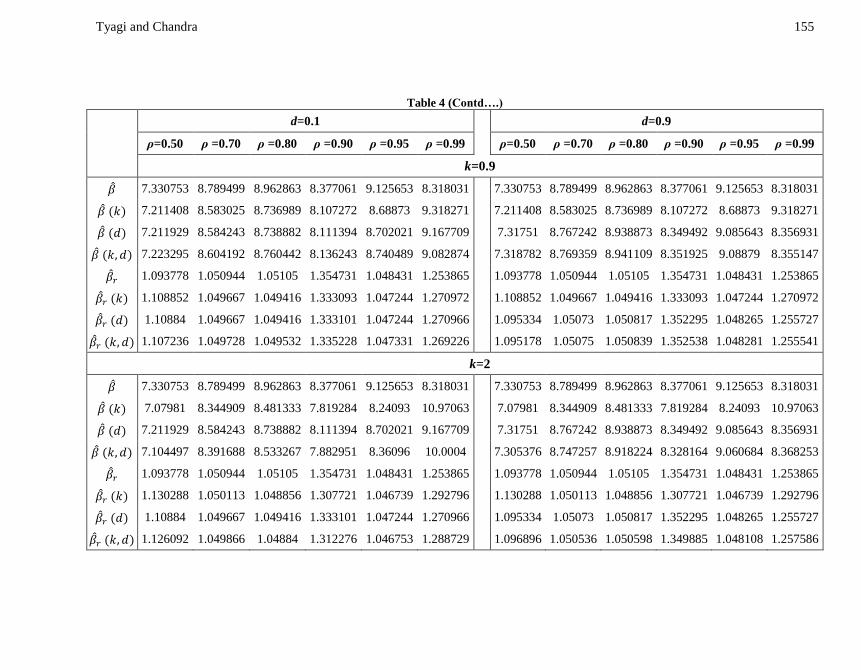
The average Mahalanobis loss in misspecified model for different values of for
and some arbitrarity selected values of and is presented in Table 4. The
results in the Table 4 exhibit that when , the PCR estimator performs better
than all the other estimators. When , for smaller values of the
class estimator outperforms the others and for larger values of the class
estimator starts dominating the other estimators. Moreover, if we examine the superiority
of the class estimator, we observe that the class estimator
outperforms all the other estimators except the PCR estimator for while
for , the class estimator dominates the OLS, ORR, Liu, two-
parameter class and the PCR estimators. Hence from these results, we can say that for
low and strong collinearity the PCR estimator is a good choice and when the
multicollinearity is moderate, the class estimator for small value of d and r-k class
estimator for large values of may be suggested for practical purposes.
Furthermore, the results show that the superiority of the estimators changes with the
value of , which is evident from the theoretical results that the dominance depends on
the sign of . In this simulation it is positive when and is
negative for . Hence, same dominance can be seen for
and ; and for other values of . Additionally it can also be verified that the
conditions of the dominance given in the theorems are also satisfied. For example in one
iteration of simulation when , the values of and are
-0.6776841 and -5.90645, resulting in positive values of (r is obtained
to be 1). Further, the eigen values of X’X matrix are 138.30927, 52.87401, 39.35769,
29.83332, 21.02597, hence the value of ⁄ for
is obtained to be 0.1935084 which is less than 1. Thus the condition in Theorem
3.6 (i) for the superiority of the class estimator over the class estimator
is satisfied which gives an evidence to the result obtained in Table 5 that the class estimator outperforms the class estimator for when .
Performance of some biased estimators in misspecified model… 148
Table 1
Simulated Average Mahalanobis Loss in Misspecified Model when
k
d=0.1 d=0.3 d=0.5 d=0.7 d=0.9 d=0.99
=45.199135, =1.090234
0.01 45.14713 45.14713 45.14713 45.14713 45.14713 45.14713
40.96507 42.04656 43.03864 43.95293 44.79905 45.15978
45.15234 45.16276 45.17316 45.18356 45.19395 45.19862
1.089961 1.089961 1.089961 1.089961 1.089961 1.089961
1.069107 1.073211 1.077653 1.082433 1.08755 1.089962
1.089988 1.090043 1.090097 1.090152 1.090207 1.090231
0.1 44.6826 44.6826 44.6826 44.6826 44.6826 44.6826
40.96507 42.04656 43.03864 43.95293 44.79905 45.15978
44.73541 44.84024 44.94404 45.04682 45.14861 45.19409
1.087542 1.087542 1.087542 1.087542 1.087542 1.087542
1.069107 1.073211 1.077653 1.082433 1.08755 1.089962
1.087807 1.088341 1.088877 1.089417 1.089961 1.090207
0.3 43.67305 43.67305 43.67305 43.67305 43.67305 43.67305
40.96507 42.04656 43.03864 43.95293 44.79905 45.15978
43.83567 44.15387 44.46304 44.76359 45.05593 45.1849
1.082416 1.082416 1.082416 1.082416 1.082416 1.082416
1.069107 1.073211 1.077653 1.082433 1.08755 1.089962
1.083163 1.084682 1.08623 1.087809 1.089418 1.090152
0.5 42.69484 42.69484 42.69484 42.69484 42.69484 42.69484
40.96507 42.04656 43.03864 43.95293 44.79905 45.15978
42.97208 43.50706 44.0177 44.50579 44.97295 45.17673
1.077634 1.077634 1.077634 1.077634 1.077634 1.077634
1.069107 1.073211 1.077653 1.082433 1.08755 1.089962
1.078799 1.081192 1.08367 1.086233 1.088879 1.090098
0.7 41.74799 41.74799 41.74799 41.74799 41.74799 41.74799
40.96507 42.04656 43.03864 43.95293 44.79905 45.15978
42.14368 42.89721 43.60456 44.27025 44.89821 45.16942
1.073195 1.073195 1.073195 1.073195 1.073195 1.073195
1.069107 1.073211 1.077653 1.082433 1.08755 1.089962
1.074713 1.077873 1.081198 1.084689 1.088344 1.090043
0.9 40.83249 40.83249 40.83249 40.83249 40.83249 40.83249
40.96507 42.04656 43.03864 43.95293 44.79905 45.15978
41.34956 42.32193 43.22057 44.05429 44.83054 45.16283
1.069101 1.069101 1.069101 1.069101 1.069101 1.069101
1.069107 1.073211 1.077653 1.082433 1.08755 1.089962
1.070906 1.074722 1.078813 1.083177 1.087814 1.089989
2 36.35766 36.35766 36.35766 36.35766 36.35766 36.35766
40.96507 42.04656 43.03864 43.95293 44.79905 45.15978
37.55609 39.68568 41.52382 43.13019 44.54914 45.13576
1.052731 1.052731 1.052731 1.052731 1.052731 1.052731
1.069107 1.073211 1.077653 1.082433 1.08755 1.089962
1.054948 1.060414 1.067247 1.075435 1.084967 1.089692
Tyagi and Chandra 149
Table 1 (Contd….)
k
d=0.1 d=0.1 d=0.1 d=0.1 d=0.1 d=0.1
=37.30482, =2.921312
0.01 37.3988 37.3988 37.3988 37.3988 37.3988 37.3988
45.81878 42.23921 40.09346 38.68299 37.69432 37.34125
37.38925 37.37024 37.35138 37.33265 37.31406 37.30574
2.92308 2.92308 2.92308 2.92308 2.92308 2.92308
3.083709 3.046953 3.010581 2.974589 2.938976 2.923074
2.922903 2.922549 2.922196 2.921842 2.921489 2.92133
0.1 38.26221 38.26221 38.26221 38.26221 38.26221 38.26221
45.81878 42.23921 40.09346 38.68299 37.69432 37.34125
38.15073 37.93949 37.74262 37.55877 37.38674 37.31289
2.939029 2.939029 2.939029 2.939029 2.939029 2.939029
3.083709 3.046953 3.010581 2.974589 2.938976 2.923074
2.937253 2.933704 2.930159 2.926617 2.923079 2.921489
0.3 40.29422 40.29422 40.29422 40.29422 40.29422 40.29422
45.81878 42.23921 40.09346 38.68299 37.69432 37.34125
39.85099 39.09176 38.46649 37.94383 37.50133 37.32381
2.974713 2.974713 2.974713 2.974713 2.974713 2.974713
3.083709 3.046953 3.010581 2.974589 2.938976 2.923074
2.969334 2.958603 2.947906 2.937242 2.926614 2.921842
0.5 42.48254 42.48254 42.48254 42.48254 42.48254 42.48254
45.81878 42.23921 40.09346 38.68299 37.69432 37.34125
41.55741 40.11351 39.04392 38.22403 37.57825 37.33089
3.01073 3.01073 3.01073 3.01073 3.01073 3.01073
3.083709 3.046953 3.010581 2.974589 2.938976 2.923074
3.001681 2.983655 2.965724 2.947888 2.930147 2.922194
0.7 44.82717 44.82717 44.82717 44.82717 44.82717 44.82717
45.81878 42.23921 40.09346 38.68299 37.69432 37.34125
43.26482 41.02851 39.51816 38.43873 37.63395 37.33591
3.04708 3.04708 3.04708 3.04708 3.04708 3.04708
3.083709 3.046953 3.010581 2.974589 2.938976 2.923074
3.034293 3.00886 2.983613 2.958553 2.933679 2.922547
0.9 47.32811 47.32811 47.32811 47.32811 47.32811 47.32811
45.81878 42.23921 40.09346 38.68299 37.69432 37.34125
44.96901 41.85482 39.91666 38.60966 37.67651 37.33969
3.083763 3.083763 3.083763 3.083763 3.083763 3.083763
3.083709 3.046953 3.010581 2.974589 2.938976 2.923074
3.06717 3.034217 3.001574 2.969239 2.937211 2.922898
2 63.87723 63.87723 63.87723 63.87723 63.87723 63.87723
45.81878 42.23921 40.09346 38.68299 37.69432 37.34125
54.15715 45.31404 41.35079 39.16787 37.80701 37.35104
3.291475 3.291475 3.291475 3.291475 3.291475 3.291475
3.083709 3.046953 3.010581 2.974589 2.938976 2.923074
3.252732 3.176406 3.10162 3.028361 2.956618 2.924826
Performance of some biased estimators in misspecified model… 150
Table 2
Simulated Average Mahalanobis Loss in Misspecified Model when
k
=0.95
=9.125653, =1.048431
0.01 9.12045 9.12045 9.12045 9.12045 9.12045 9.12045
8.702021 8.810268 8.909543 9.001012 9.085643 9.121717
9.120971 9.122013 9.123055 9.124095 9.125134 9.125601
1.048414 1.048414 1.048414 1.048414 1.048414 1.048414
1.047244 1.047448 1.047686 1.047959 1.048265 1.048414
1.048415 1.048419 1.048422 1.048425 1.048429 1.04843
0.1 9.073971 9.073971 9.073971 9.073971 9.073971 9.073971
8.702021 8.810268 8.909543 9.001012 9.085643 9.121717
9.079255 9.089744 9.10013 9.110414 9.120598 9.125149
1.048264 1.048264 1.048264 1.048264 1.048264 1.048264
1.047244 1.047448 1.047686 1.047959 1.048265 1.048414
1.048281 1.048313 1.048346 1.04838 1.048414 1.048429
0.3 8.972958 8.972958 8.972958 8.972958 8.972958 8.972958
8.702021 8.810268 8.909543 9.001012 9.085643 9.121717
8.989232 9.021073 9.052009 9.08208 9.111327 9.124229
1.047958 1.047958 1.047958 1.047958 1.047958 1.047958
1.047244 1.047448 1.047686 1.047959 1.048265 1.048414
1.048001 1.048091 1.048184 1.048281 1.04838 1.048425
0.5 8.87508 8.87508 8.87508 8.87508 8.87508 8.87508
8.702021 8.810268 8.909543 9.001012 9.085643 9.121717
8.902826 8.956364 9.00746 9.056294 9.103028 9.123412
1.047685 1.047685 1.047685 1.047685 1.047685 1.047685
1.047244 1.047448 1.047686 1.047959 1.048265 1.048414
1.04775 1.047886 1.048031 1.048185 1.048346 1.048422
0.7 8.780337 8.780337 8.780337 8.780337 8.780337 8.780337
8.702021 8.810268 8.909543 9.001012 9.085643 9.121717
8.819943 8.895357 8.966137 9.032738 9.095554 9.122681
1.047447 1.047447 1.047447 1.047447 1.047447 1.047447
1.047244 1.047448 1.047686 1.047959 1.048265 1.048414
1.047527 1.047698 1.047887 1.048092 1.048313 1.048419
0.9 8.68873 8.68873 8.68873 8.68873 8.68873 8.68873
8.702021 8.810268 8.909543 9.001012 9.085643 9.121717
8.740489 8.837812 8.927735 9.011145 9.08879 9.122022
1.047244 1.047244 1.047244 1.047244 1.047244 1.047244
1.047244 1.047448 1.047686 1.047959 1.048265 1.048414
1.047331 1.047527 1.047751 1.048002 1.048281 1.048415
2 8.24093 8.24093 8.24093 8.24093 8.24093 8.24093
8.702021 8.810268 8.909543 9.001012 9.085643 9.121717
8.36096 8.574176 8.758126 8.91881 9.060684 9.119319
1.046739 1.046739 1.046739 1.046739 1.046739 1.046739
1.047244 1.047448 1.047686 1.047959 1.048265 1.048414
1.046753 1.046887 1.047158 1.047565 1.048108 1.048397
Tyagi and Chandra 151
Table 2 (Contd….)
k
=0.99
=8.318031, =1.253865
0.01 8.327405 8.327405 8.327405 8.327405 8.327405 8.327405
9.167709 8.810531 8.596413 8.455639 8.356931 8.32167
8.326452 8.324557 8.322675 8.320807 8.318953 8.318123
1.254052 1.254052 1.254052 1.254052 1.254052 1.254052
1.270966 1.267099 1.26327 1.25948 1.255727 1.254051
1.254033 1.253996 1.253959 1.253921 1.253884 1.253867
0.1 8.413538 8.413538 8.413538 8.413538 8.413538 8.413538
9.167709 8.810531 8.596413 8.455639 8.356931 8.32167
8.402417 8.381345 8.361706 8.343365 8.326203 8.318836
1.255733 1.255733 1.255733 1.255733 1.255733 1.255733
1.270966 1.267099 1.26327 1.25948 1.255727 1.254051
1.255546 1.255172 1.254798 1.254425 1.254052 1.253884
0.3 8.616275 8.616275 8.616275 8.616275 8.616275 8.616275
9.167709 8.810531 8.596413 8.455639 8.356931 8.32167
8.572058 8.496316 8.433937 8.381791 8.337639 8.319925
1.259493 1.259493 1.259493 1.259493 1.259493 1.259493
1.270966 1.267099 1.26327 1.25948 1.255727 1.254051
1.258926 1.257795 1.256668 1.255545 1.254424 1.253921
0.5 8.834643 8.834643 8.834643 8.834643 8.834643 8.834643
9.167709 8.810531 8.596413 8.455639 8.356931 8.32167
8.742344 8.59829 8.491575 8.409767 8.345322 8.320633
1.263286 1.263286 1.263286 1.263286 1.263286 1.263286
1.270966 1.267099 1.26327 1.25948 1.255727 1.254051
1.262333 1.260435 1.258546 1.256666 1.254797 1.253958
0.7 9.068642 9.068642 9.068642 9.068642 9.068642 9.068642
9.167709 8.810531 8.596413 8.455639 8.356931 8.32167
8.912758 8.689633 8.538933 8.431216 8.350889 8.321135
1.267112 1.267112 1.267112 1.267112 1.267112 1.267112
1.270966 1.267099 1.26327 1.25948 1.255727 1.254051
1.265766 1.263089 1.26043 1.25779 1.255169 1.253996
0.9 9.318271 9.318271 9.318271 9.318271 9.318271 9.318271
9.167709 8.810531 8.596413 8.455639 8.356931 8.32167
9.082874 8.772142 8.578744 8.448304 8.355147 8.321513
1.270972 1.270972 1.270972 1.270972 1.270972 1.270972
1.270966 1.267099 1.26327 1.25948 1.255727 1.254051
1.269226 1.265758 1.262322 1.258916 1.255541 1.254033
2 10.97063 10.97063 10.97063 10.97063 10.97063 10.97063
9.167709 8.810531 8.596413 8.455639 8.356931 8.32167
10.0004 9.117806 8.722217 8.504241 8.368253 8.322654
1.292796 1.292796 1.292796 1.292796 1.292796 1.292796
1.270966 1.267099 1.26327 1.25948 1.255727 1.254051
1.288729 1.280712 1.27285 1.265142 1.257586 1.254236
Performance of some biased estimators in misspecified model… 152
Table 3
Simulated Average Mahalanobis Loss in Misspecified Model when
k
=0.95
=5.493342, =1.046878
0.01 5.492821 5.492821 5.492821 5.492821 5.492821 5.492821
5.450908 5.461763 5.471712 5.480872 5.489341 5.492949
5.492873 5.492978 5.493082 5.493186 5.49329 5.493337
1.04688 1.04688 1.04688 1.04688 1.04688 1.04688
1.047052 1.047008 1.046966 1.046928 1.046894 1.04688
1.04688 1.046879 1.046879 1.046879 1.046878 1.046878
0.1 5.488165 5.488165 5.488165 5.488165 5.488165 5.488165
5.450908 5.461763 5.471712 5.480872 5.489341 5.492949
5.488694 5.489745 5.490786 5.491816 5.492836 5.493292
1.046894 1.046894 1.046894 1.046894 1.046894 1.046894
1.047052 1.047008 1.046966 1.046928 1.046894 1.04688
1.046892 1.046889 1.046886 1.046883 1.04688 1.046878
0.3 5.478046 5.478046 5.478046 5.478046 5.478046 5.478046
5.450908 5.461763 5.471712 5.480872 5.489341 5.492949
5.479677 5.482867 5.485967 5.488979 5.491908 5.4932
1.046929 1.046929 1.046929 1.046929 1.046929 1.046929
1.047052 1.047008 1.046966 1.046928 1.046894 1.04688
1.046923 1.046913 1.046902 1.046892 1.046883 1.046879
0.5 5.46824 5.46824 5.46824 5.46824 5.46824 5.46824
5.450908 5.461763 5.471712 5.480872 5.489341 5.492949
5.471021 5.476388 5.481507 5.486399 5.491078 5.493118
1.046966 1.046966 1.046966 1.046966 1.046966 1.046966
1.047052 1.047008 1.046966 1.046928 1.046894 1.04688
1.046957 1.046938 1.04692 1.046902 1.046886 1.046879
0.7 5.458747 5.458747 5.458747 5.458747 5.458747 5.458747
5.450908 5.461763 5.471712 5.480872 5.489341 5.492949
5.462719 5.47028 5.477372 5.484043 5.490331 5.493045
1.047008 1.047008 1.047008 1.047008 1.047008 1.047008
1.047052 1.047008 1.046966 1.046928 1.046894 1.04688
1.046993 1.046964 1.046938 1.046913 1.046889 1.046879
0.9 5.449568 5.449568 5.449568 5.449568 5.449568 5.449568
5.450908 5.461763 5.471712 5.480872 5.489341 5.492949
5.454761 5.46452 5.473531 5.481884 5.489655 5.492979
1.047052 1.047052 1.047052 1.047052 1.047052 1.047052
1.047052 1.047008 1.046966 1.046928 1.046894 1.04688
1.047032 1.046993 1.046956 1.046923 1.046892 1.04688
2 5.404688 5.404688 5.404688 5.404688 5.404688 5.404688
5.450908 5.461763 5.471712 5.480872 5.489341 5.492949
5.41675 5.438153 5.456591 5.472675 5.486855 5.49271
1.04736 1.04736 1.04736 1.04736 1.04736 1.04736
1.047052 1.047008 1.046966 1.046928 1.046894 1.04688
1.047296 1.047179 1.047075 1.046986 1.046911 1.046881

Tyagi and Chandra 153
Table 3 (Contd….)
k
=0.99
=5.405501, =1.073579
0.01 5.406432 5.406432 5.406432 5.406432 5.406432 5.406432
5.489926 5.454455 5.433187 5.419196 5.409376 5.405864
5.406337 5.406149 5.405962 5.405777 5.405593 5.405511
1.0736 1.0736 1.0736 1.0736 1.0736 1.0736
1.075561 1.075114 1.07467 1.074231 1.073795 1.0736
1.073598 1.073594 1.073589 1.073585 1.073581 1.073579
0.1 5.414979 5.414979 5.414979 5.414979 5.414979 5.414979
5.489926 5.454455 5.433187 5.419196 5.409376 5.405864
5.413875 5.411784 5.409836 5.408016 5.406312 5.405581
1.073796 1.073796 1.073796 1.073796 1.073796 1.073796
1.075561 1.075114 1.07467 1.074231 1.073795 1.0736
1.073774 1.07373 1.073687 1.073644 1.0736 1.073581
0.3 5.435106 5.435106 5.435106 5.435106 5.435106 5.435106
5.489926 5.454455 5.433187 5.419196 5.409376 5.405864
5.430718 5.423201 5.417009 5.411833 5.407449 5.40569
1.074232 1.074232 1.074232 1.074232 1.074232 1.074232
1.075561 1.075114 1.07467 1.074231 1.073795 1.0736
1.074166 1.074035 1.073904 1.073774 1.073643 1.073585
0.5 5.456796 5.456796 5.456796 5.456796 5.456796 5.456796
5.489926 5.454455 5.433187 5.419196 5.409376 5.405864
5.447634 5.433335 5.42274 5.414617 5.408214 5.40576
1.074672 1.074672 1.074672 1.074672 1.074672 1.074672
1.075561 1.075114 1.07467 1.074231 1.073795 1.0736
1.074561 1.074341 1.074122 1.073904 1.073687 1.073589
0.7 5.480049 5.480049 5.480049 5.480049 5.480049 5.480049
5.489926 5.454455 5.433187 5.419196 5.409376 5.405864
5.464572 5.442419 5.427455 5.416755 5.40877 5.40581
1.075115 1.075115 1.075115 1.075115 1.075115 1.075115
1.075561 1.075114 1.07467 1.074231 1.073795 1.0736
1.074959 1.074649 1.074341 1.074034 1.07373 1.073594
0.9 5.504865 5.504865 5.504865 5.504865 5.504865 5.504865
5.489926 5.454455 5.433187 5.419196 5.409376 5.405864
5.481488 5.450632 5.431424 5.418462 5.409197 5.405848
1.075562 1.075562 1.075562 1.075562 1.075562 1.075562
1.075561 1.075114 1.07467 1.074231 1.073795 1.0736
1.07536 1.074958 1.07456 1.074165 1.073773 1.073598
2 5.669295 5.669295 5.669295 5.669295 5.669295 5.669295
5.489926 5.454455 5.433187 5.419196 5.409376 5.405864
5.572832 5.485116 5.44579 5.424093 5.410525 5.405964
1.078077 1.078077 1.078077 1.078077 1.078077 1.078077
1.075561 1.075114 1.07467 1.074231 1.073795 1.0736
1.077609 1.076686 1.075779 1.074887 1.074011 1.073622
Performance of some biased estimators in misspecified model… 154
Table 4
Simulated Average Mahalanobis Loss in Misspecified Model for Different ρ when
d=0.1
d=0.9
ρ=0.50 ρ =0.70 ρ =0.80 ρ =0.90 ρ =0.95 ρ =0.99
ρ=0.50 ρ =0.70 ρ =0.80 ρ =0.90 ρ =0.95 ρ =0.99
k=0.1
7.330753 8.789499 8.962863 8.377061 9.125653 8.318031
7.330753 8.789499 8.962863 8.377061 9.125653 8.318031
7.316974 8.76604 8.937024 8.345566 9.073971 8.413538
7.316974 8.76604 8.937024 8.345566 9.073971 8.413538
7.211929 8.584243 8.738882 8.111394 8.702021 9.167709
7.31751 8.767242 8.938873 8.349492 9.085643 8.356931
7.318352 8.768393 8.93962 8.348744 9.079255 8.402417
7.329375 8.78716 8.960291 8.37394 9.120598 8.326203
1.093778 1.050944 1.05105 1.354731 1.048431 1.253865
1.093778 1.050944 1.05105 1.354731 1.048431 1.253865
1.095344 1.050729 1.050816 1.352287 1.048264 1.255733
1.095344 1.050729 1.050816 1.352287 1.048264 1.255733
1.10884 1.049667 1.049416 1.333101 1.047244 1.270966
1.095334 1.05073 1.050817 1.352295 1.048265 1.255727
1.095186 1.05075 1.050839 1.352531 1.048281 1.255546
1.093933 1.050922 1.051026 1.354486 1.048414 1.254052
k=0.5
7.330753 8.789499 8.962863 8.377061 9.125653 8.318031
7.330753 8.789499 8.962863 8.377061 9.125653 8.318031
7.263153 8.673497 8.835522 8.223383 8.87508 8.834643
7.263153 8.673497 8.835522 8.223383 8.87508 8.834643
7.211929 8.584243 8.738882 8.111394 8.702021 9.167709
7.31751 8.767242 8.938873 8.349492 9.085643 8.356931
7.269903 8.685263 8.848535 8.239411 8.902826 8.742344
7.323984 8.778063 8.950402 8.362324 9.103028 8.345322
1.093778 1.050944 1.05105 1.354731 1.048431 1.253865
1.093778 1.050944 1.05105 1.354731 1.048431 1.253865
1.101879 1.050052 1.050011 1.342612 1.047685 1.263286
1.101879 1.050052 1.050011 1.342612 1.047685 1.263286
1.10884 1.049667 1.049416 1.333101 1.047244 1.270966
1.095334 1.05073 1.050817 1.352295 1.048265 1.255727
1.101035 1.050121 1.050101 1.343815 1.04775 1.262333
1.094555 1.050834 1.050931 1.35351 1.048346 1.254797
Tyagi and Chandra 155
Table 4 (Contd….)
d=0.1
d=0.9
ρ=0.50 ρ =0.70 ρ =0.80 ρ =0.90 ρ =0.95 ρ =0.99
ρ=0.50 ρ =0.70 ρ =0.80 ρ =0.90 ρ =0.95 ρ =0.99
k=0.9
7.330753 8.789499 8.962863 8.377061 9.125653 8.318031
7.330753 8.789499 8.962863 8.377061 9.125653 8.318031
7.211408 8.583025 8.736989 8.107272 8.68873 9.318271
7.211408 8.583025 8.736989 8.107272 8.68873 9.318271
7.211929 8.584243 8.738882 8.111394 8.702021 9.167709
7.31751 8.767242 8.938873 8.349492 9.085643 8.356931
7.223295 8.604192 8.760442 8.136243 8.740489 9.082874
7.318782 8.769359 8.941109 8.351925 9.08879 8.355147
1.093778 1.050944 1.05105 1.354731 1.048431 1.253865
1.093778 1.050944 1.05105 1.354731 1.048431 1.253865
1.108852 1.049667 1.049416 1.333093 1.047244 1.270972
1.108852 1.049667 1.049416 1.333093 1.047244 1.270972
1.10884 1.049667 1.049416 1.333101 1.047244 1.270966
1.095334 1.05073 1.050817 1.352295 1.048265 1.255727
1.107236 1.049728 1.049532 1.335228 1.047331 1.269226
1.095178 1.05075 1.050839 1.352538 1.048281 1.255541
k=2
7.330753 8.789499 8.962863 8.377061 9.125653 8.318031
7.330753 8.789499 8.962863 8.377061 9.125653 8.318031
7.07981 8.344909 8.481333 7.819284 8.24093 10.97063
7.07981 8.344909 8.481333 7.819284 8.24093 10.97063
7.211929 8.584243 8.738882 8.111394 8.702021 9.167709
7.31751 8.767242 8.938873 8.349492 9.085643 8.356931
7.104497 8.391688 8.533267 7.882951 8.36096 10.0004
7.305376 8.747257 8.918224 8.328164 9.060684 8.368253
1.093778 1.050944 1.05105 1.354731 1.048431 1.253865
1.093778 1.050944 1.05105 1.354731 1.048431 1.253865
1.130288 1.050113 1.048856 1.307721 1.046739 1.292796
1.130288 1.050113 1.048856 1.307721 1.046739 1.292796
1.10884 1.049667 1.049416 1.333101 1.047244 1.270966
1.095334 1.05073 1.050817 1.352295 1.048265 1.255727
1.126092 1.049866 1.04884 1.312276 1.046753 1.288729
1.096896 1.050536 1.050598 1.349885 1.048108 1.257586
Performance of some biased estimators in misspecified model… 156
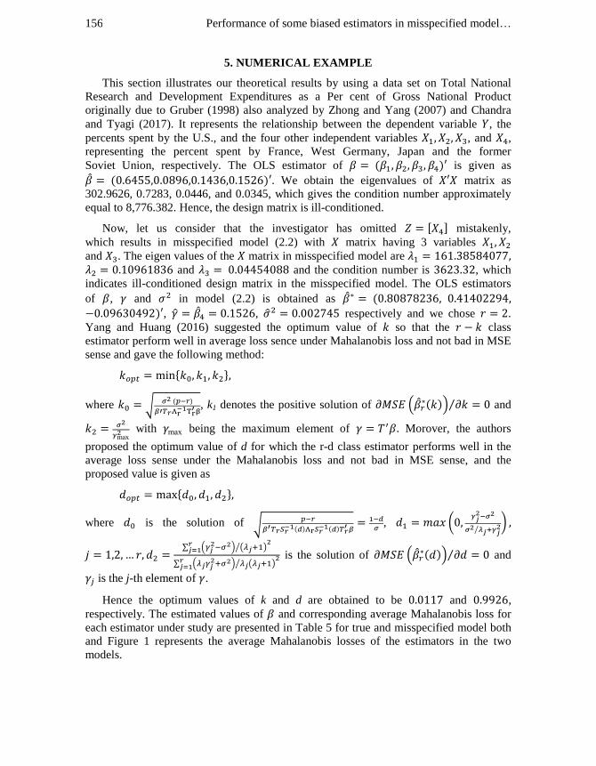
5. NUMERICAL EXAMPLE
This section illustrates our theoretical results by using a data set on Total National
Research and Development Expenditures as a Per cent of Gross National Product
originally due to Gruber (1998) also analyzed by Zhong and Yang (2007) and Chandra
and Tyagi (2017). It represents the relationship between the dependent variable , the
percents spent by the U.S., and the four other independent variables , and ,
representing the percent spent by France, West Germany, Japan and the former
Soviet Union, respectively. The OLS estimator of is given as
. We obtain the eigenvalues of matrix as
302.9626, 0.7283, 0.0446, and 0.0345, which gives the condition number approximately
equal to 8,776.382. Hence, the design matrix is ill-conditioned.
Now, let us consider that the investigator has omitted [ ] mistakenly,
which results in misspecified model (2.2) with matrix having 3 variables
and . The eigen values of the matrix in misspecified model are and and the condition number is , which
indicates ill-conditioned design matrix in the misspecified model. The OLS estimators
of , and in model (2.2) is obtained as
, , respectively and we chose .
Yang and Huang (2016) suggested the optimum value of so that the class
estimator perform well in average loss sence under Mahalanobis loss and not bad in MSE
sense and gave the following method:
{ }
where √
, k1 denotes the positive solution of (
) ⁄ and
ma with ma being the maximum element of Morover, the authors
proposed the optimum value of d for which the r-d class estimator performs well in the
average loss sense under the Mahalanobis loss and not bad in MSE sense, and the
proposed value is given as
{ }
where is the solution of √
, (
⁄ )
∑ (
) ( )
⁄
∑ ( ) ( )
⁄
is the solution of ( ) ⁄ and
is the j-th element of .
Hence the optimum values of k and d are obtained to be and ,
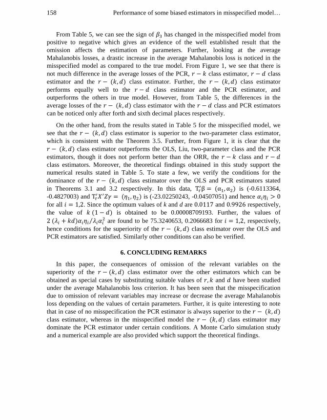
respectively. The estimated values of and corresponding average Mahalanobis loss for
each estimator under study are presented in Table 5 for true and misspecified model both
and Figure 1 represents the average Mahalanobis losses of the estimators in the two
models.

Tyagi and Chandra 157
Table 5: Estimated Values of Regression Coefficients and Average
Malahanobis Loss (Avg. ML) for True and Misspecified Model
True Model Misspecified Model
Avg. ML Avg. ML
0.6455 0.0896 0.1436 0.1526 3.0000000 0.8088 0.4140 -0.0963 1206.00734
0.5511 0.1156 0.1800 0.1633 3.3665774 0.7155 0.4387 -0.0427 1203.88878
0.6422 0.0905 0.1442 0.1534 3.0006518 0.8053 0.4139 -0.0932 1205.43413
0.6448 0.0898 0.1438 0.1527 3.0000137 0.8081 0.4142 -0.0959 1205.99025
0.2100 0.2401 0.3047 0.1861 2.0000000 0.4090 0.6627 -0.0161 1205.00629
0.2092 0.2395 0.3029 0.1880 2.1076093 0.3994 0.6354 0.0207 1202.66200
0.2098 0.2399 0.3042 0.1866 2.0004638 0.4083 0.6608 -0.0136 1204.43378
0.2100 0.2401 0.3047 0.1861 2.0000048 0.4089 0.6625 -0.0159 1204.98938
(a)
(b)
Figure 1: Average Mahalanobis Loss of the estimators
(a) In Case of No Misspecification, (b) When there is Misspecification
Performance of some biased estimators in misspecified model… 158
From Table 5, we can see the sign of has changed in the misspecified model from
positive to negative which gives an evidence of the well established result that the
omission affects the estimation of parameters. Further, looking at the average
Mahalanobis losses, a drastic increase in the average Mahalanobis loss is noticed in the
misspecified model as compared to the true model. From Figure 1, we see that there is
not much difference in the average losses of the PCR, class estimator, class
estimator and the class estimator. Further, the class estimator
performs equally well to the class estimator and the PCR estimator, and
outperforms the others in true model. However, from Table 5, the differences in the
average losses of the class estimator with the class and PCR estimators
can be noticed only after forth and sixth decimal places respectively.
On the other hand, from the results stated in Table 5 for the misspecified model, we
see that the class estimator is superior to the two-parameter class estimator,
which is consistent with the Theorem 3.5. Further, from Figure 1, it is clear that the
class estimator outperforms the OLS, Liu, two-parameter class and the PCR
estimators, though it does not perform better than the ORR, the class and
class estimators. Moreover, the theoretical findings obtained in this study support the
numerical results stated in Table 5. To state a few, we verify the conditions for the
dominance of the class estimator over the OLS and PCR estimators stated
in Theorems 3.1 and 3.2 respectively. In this data, is (-0.6113364,
-0.4827003) and is (-23.02250243, -0.04507051) and hence
for all . Since the optimum values of k and d are and respectively,
the value of is obtained to be 0.00008709193. Further, the values of
⁄ are found to be 75.3240653, 0.2066683 for , respectively,
hence conditions for the superiority of the class estimator over the OLS and
PCR estimators are satisfied. Similarly other conditions can also be verified.
6. CONCLUDING REMARKS
In this paper, the consequences of omission of the relevant variables on the
superiority of the class estimator over the other estimators which can be
obtained as special cases by substituting suitable values of and have been studied
under the average Mahalanobis loss criterion. It has been seen that the misspecification
due to omission of relevant variables may increase or decrease the average Mahalanobis
loss depending on the values of certain parameters. Further, it is quite interesting to note
that in case of no misspecification the PCR estimator is always superior to the
class estimator, whereas in the misspecified model the class estimator may
dominate the PCR estimator under certain conditions. A Monte Carlo simulation study
and a numerical example are also provided which support the theoretical findings.
Tyagi and Chandra 159
REFERENCES
1. Baye, M.R. and Parker, D.F. (1984). Combining ridge and principal component
regression: A money demand illustration. Communications in Statistics-Theory and
Methods, 13, 197-205.
2. Chandra, S. and Tyagi, G. (2017). On the performance of the biased estimators in a
misspecified model with correlated regressors, Statistics in Transition-new series,
18(1).
3. iray, G.Ü., Kaçiranlar, S. and Sakallio lu, S. (2012). class estimator in the
linear regression model with correlated errors. Statistical Papers, 55(2), 393-407.
doi: 10.1007/s00362-012-0484-8.
4. iray, G.Ü. (2015). class estimator under misspecification. Communications in
Statistics - Theory and Methods, 44, 4742-4756.
5. Dube, M., Srivastava, V.K., Toutenburg, H. and Wijekoon, P. (1991). Stein-rule
estimator under inclusion of superfluous variables in linear regression models.
Communications in Statistics - Theory and Methods, 20, 2009-2022.
6. Dube, M. (1999). Mixed regression estimator under inclusion of some superfluous
variables. Test, 8, 411-418.
7. Gibbons, D.G. (1981). A simulation study of some ridge estimators. Journal of the
American Statistical Association, 76, 131-139.
8. Groß, J., Trenkler, G. and Liski, E.P. (1998). Necessary and sufficient conditions for
superiority of misspecified restricted least squares regression estimator. Journal of
Statistical Planning and Inference, 71, 109-116.
9. Gruber, M. (1998). Improving efficiency by shrinkage: The james-stein and ridge
regression estimator. Marcel Dekker, Inc., New York.
10. Hoerl, A.E. and Kennard, R.W. (1970). Ridge regression: Biased estimation for non-
orthogonal problems. Technometrics, 12, 55-67.
11. Hubert, M. and Wijekoon, P. (2004). Superiority of the stochastic restricted liu
estimator under misspecification. Statistica, 64, 153-162.
12. Jianwen, X. and Hu, Y. (2012). On the stochastic restricted liu estimator under
misspecification due to inclusion of some superfluous variables. Chinese journal of
applied probability and statistics, 28, 123-133.
13. Johnston, J. and DiNardo, J. (1997). Econometric methods. Mc-Graw Hill, forth edn.
14. Kaçiranlar, S. and Sakallio lu, S. (2001). Combining the liu estimator and the
principal component regression estimator. Communications in Statistics-Theory and
Methods, 30, 2699-2705.
15. Kadiyala, K. (1986). Mixed regression estimator under misspecification. Economic
Letters, 21, 27-30.
16. Liu, K. (1993). A new class of biased estimate in linear regression. Communications
in Statistics-Theory and Methods, 22, 393-402.
17. Mahalanobis, P.C. (1936). On the generalized distance in the statistics. Proc.Nat.
Instit. Sci. India, 12, 49-55.
18. Massy, W.F. (1965). Principal components regression in exploratory statistical
research. Journal of the American Statistical Association, 60, 234-256.
19. McDonald, G.C. and Galarneau, D.I. (1975). A monte carlo evaluation of some ridge-
type estimators. Journal of the American Statistical Association, 70, 407-416.

Performance of some biased estimators in misspecified model… 160
20. Nomura, M. and Ohkubo, T. (1985). A note on combining ridge and principal
component regression. Communications in Statistics- Theory and Methods, 14,
2489-2493.
21. Özkale, M.R. and Kaçiranlar, S. (2007). The restricted and unrestricted two parameter
estimators. Communications in Statistics- Theory and Methods, 36, 2707-2725.
22. Özkale, M.R. (2012). Combining the unrestricted estimators into a single estimator
and a simulation study on the unrestricted estimators. Journal of Statistical
Computation and Simulation, 82, 653-688.
23. Peddada, S., Nigam, A. and Saxena, A. (1989). On the inadmssibility of ridge
estimator in a linear model. Communications in Statistics - Theory and Methods, 18,
3571-3585.
24. Chandra, S. and Sarkar, N. (2015). Comparison of the class estimator with
some estimators for multicollinearity under the Mahalanobis loss function.
International Econometric Review (IER), 7(1), 1-12.
25. Sarkar, N. (1989). Comparisons among some estimators in misspecified linear models
with multicollinearity. Annals of Institute of Statistical Methods, 41, 717-724.
26. Sarkar, N. (1996). Mean square error matrix comparison of some estimators in linear
regressions with multicollinearity. Statistics & Probability Letters, 30, 133-138.
27. Uemukai, R. (2010). Small sample properties of a ridge regression estimator when
there exist omitted variables. Statistical Papers, 52, 953-969.
28. Wijekoon, P. and Trenkler, G. (1989). Mean squared error matrix superiority of
estimators under linear restrictions and misspecification. Economics Letters, 30,
141-149.
29. Wu, J. (2016). Superiority of the r-k class estimator over some estimators in a
misspecified linear model. Communications in Statistics - Theory and Methods, 45,
1453-1458.
30. Yang, H. and Huang, J. (2016). Further research on the principal component two-
parameter estimator in linear model. Communications in Statistics-Theory and
Methods, 45, 566-576.
31. Zhong, Z. and Yang, H. (2007). Ridge estimation to the restricted linear model.
Communications in Statistics-Theory and Methods, 36, 2099-2115.