Paper No. 9084 - Institute for Corrosion and Multiphase ... · Linear polarization resistance (LPR) and weight loss ... The corrosion rate eventually reached a stable value due to

Corrosion Behavior of Mild Steel in Sour Environments at Elevated Temperatures

Shujun Gao, Peng Jin, Bruce Brown, David Young, Srdjan Nesic, Marc Singer Institute for Corrosion and Multiphase Technology,

Department of Chemical & Biomolecular Engineering, Ohio University 342 West State Street

Athens, OH, 45701 USA

ABSTRACT

The objective of this work was to determine the corrosion rate of mild steel and characterize the

corrosion products in sour environments at temperatures ranging from 80C to 200C. First, a H2S-H2O water chemistry model was developed based on available literature for a closed system at high

temperature. Then, H2S corrosion tests were conducted at 80C, 120C, 160C and 200C with an exposure time of 4 days. Linear polarization resistance (LPR) and weight loss (WL) methods were used to measure the corrosion rates. X-ray diffraction (XRD) and scanning electron microscopy with energy dispersive X-ray spectroscopy microanalysis (SEM/EDS) were employed to characterize the corrosion products and surface morphology. The results show that the initial corrosion rates increased with temperature then decreased as they achieved steady-state. The corrosion product was comprised of two distinct layers. The inner corrosion product was always an iron oxide layer (hypothesized to be Fe3O4), while mackinawite, troilite, pyrrhotite and pyrite were identified as the main components of the

outer layer at 80C, 120C, 160C and 200C, respectively. Pourbaix diagrams generated based on the analysis of water chemistry corroborated the experimental characterization of the corrosion products. Key words: hydrogen sulfide, high temperature corrosion, iron sulfide, iron oxide

INTRODUCTION As geologic environments associated with oil and gas production have become increasingly aggressive, aqueous corrosion at higher temperatures in the presence of hydrogen sulfide (H2S) is more frequently encountered.Error! Reference source not found.-3 High temperatures and high pressures in combination with H2S lead to many materials selection and engineering challenges, as well as potential for pipeline and equipment failures, especially in downhole environments.

H2S corrosion at low temperatures (< 80C) has been widely studied,4-6 and significant progress has been made to elucidate the general corrosion mechanisms involved. As a result, kinetic and thermodynamic models have been built and verified. It is known that the initial “bare steel” corrosion rate increases with temperature, but the increase of cathodic current is more significant than that of the anodic current.7 When conditions are favorable for the formation of a corrosion product layer, its

characteristics are strongly dependent on temperature. At 25C, a porous and non-protective mackinawite layer forms on the steel surface. At 80oC, a dense and adherent corrosion product layer,

1

Paper No.

9084

©2017 by NACE International.Requests for permission to publish this manuscript in any form, in part or in whole, must be in writing toNACE International, Publications Division, 15835 Park Ten Place, Houston, Texas 77084.The material presented and the views expressed in this paper are solely those of the author(s) and are not necessarily endorsed by the Association.

composed of mackinawite and pyrrhotite, forms that confers good protectiveness.8 Temperature can accelerate both the rates of corrosion as well as the rate of corrosion product layer formation. Consequently, a peak in corrosion rate is often observed when increasing the temperature at a fixed pH2S.9 At elevated temperatures, sour corrosion has not been investigated thoroughly and the associated corrosion mechanisms are poorly understood. Until now, only a couple papers can be found on the subject in the open literature.10,11 One was published more than 20 years ago and according to the

authors, the corrosion rate at 220C decreased with time due to iron sulfide growth controlled by direct reaction of H2S with the metal surface. The corrosion rate eventually reached a stable value due to the balance between layer growth and metal dissolution. Under these conditions, the major corrosion product was identified as pyrrhotite, while traces of pyrite were present. Magnetite was also identified close to the steel surface, but the authors stated that only traces could be detected.10 Another more

recent study identified pyrrhotite at 130C by characterization using scanning electron microscopy (SEM) and transmission electron microscopy (TEM).11 Overall, it is expected that high temperature has a significant effect on:12-14

Corrosion rate.

Formation of iron sulfide polymorphs and related phases.

Phase transformations.

Observed phases may also have interactions that lead to surface heterogeneity, onset of galvanic corrosion and localized attack. Due to a lack of high temperature dats, both the kinetic and thermodynamic models for sour

environments have been verified only up to 80C.8,15 In comparison, similar models for CO2

environments have already been validated for up to 250C. It has also been reported that magnetite can form at high temperature in CO2 environments and can significantly slow down the corrosion rate.16 Whether or not the same same is true for H2S environments is unknown. Therefore, in order to understand, predict and mitigate H2S corrosion in oil and gas production at elevated temperatures, further experimental investigations and subsequent construction of new models of H2S corrosion are a necessity. In this work, a water chemistry model for a H2S-H2O system in a closed system at high temperatures was initially developed to better understand the water chemistry and help to properly adjust the relevant parameters in order to achieve the desired environmental conditions at a given temperature. H2S corrosion tests were then conducted at 80°C, 120°C, 160°C and 200°C, to identify the effect of high temperature on the kinetics of corrosion and layer formation on mild steel in sour environments.

EXPERIMENTAL PROCEDURE Experiments were performed in a 7 L Hastelloy autoclave, shown in Figure 1. A conventional three-electrode setup was used to conduct linear polarization resistance (LPR) measurements using a potentiostat. The working electrode was a cylindrical sample made from UNS K03014 (API 5L X65) carbon steel, its chemical composition shown in Table 1. A Pt-coated Nb counter electrode and a commercial Zr/ZrO2 high temperature, high pressure pH probe was used as a pseudo reference electrode. The pH probe’s reference serves as a reference electrode (exact potential still unknown) as

long as its potential is stable at the desired test conditions.16 Four flat 10102 mm samples were also attached to a stabilized shaft using a PTFE-coated 304SS wire. A centrally located impeller was used to keep the solution fully mixed during each test.

2


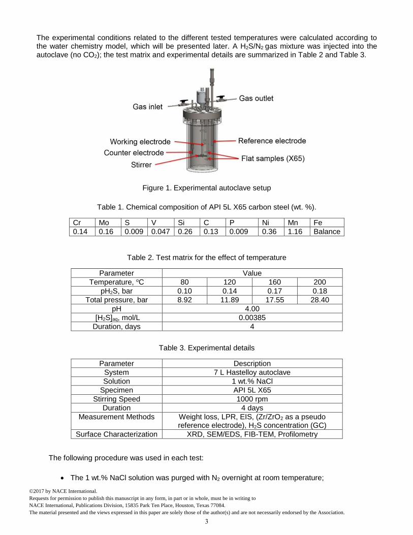
The experimental conditions related to the different tested temperatures were calculated according to the water chemistry model, which will be presented later. A H2S/N2 gas mixture was injected into the autoclave (no CO2); the test matrix and experimental details are summarized in Table 2 and Table 3.

Figure 1. Experimental autoclave setup

Table 1. Chemical composition of API 5L X65 carbon steel (wt. %).

Cr Mo S V Si C P Ni Mn Fe

0.14 0.16 0.009 0.047 0.26 0.13 0.009 0.36 1.16 Balance

Table 2. Test matrix for the effect of temperature

Parameter Value

Temperature, oC 80 120 160 200

pH2S, bar 0.10 0.14 0.17 0.18

Total pressure, bar 8.92 11.89 17.55 28.40

pH 4.00

[H2S]aq, mol/L 0.00385

Duration, days 4

Table 3. Experimental details

Parameter Description

System 7 L Hastelloy autoclave

Solution 1 wt.% NaCl

Specimen API 5L X65

Stirring Speed 1000 rpm

Duration 4 days

Measurement Methods Weight loss, LPR, EIS, (Zr/ZrO2 as a pseudo reference electrode), H2S concentration (GC)

Surface Characterization XRD, SEM/EDS, FIB-TEM, Profilometry

The following procedure was used in each test:

The 1 wt.% NaCl solution was purged with N2 overnight at room temperature;

3


pH was adjusted to the calculated initial condition by using a deareated HCl solution (1 M) (see Table 2);

The API 5L X65 samples were mounted onto the autoclave lid and put into place;

The electrolyte was further deoxygenated by purging with N2 for another 1 hour (to avoid oxygen contamination during pH adjustment);

The gas-out valve was closed and N2 was used to pressurize the system to ensure there were no leaks;

The system was then depressurized and H2S was rapidly introduced to the desired pressure (see Table 2);

The autoclave was then heated up to the desired temperature in a stepwise manner to avoid overheating;

After reaching the targeted experimental temperature, LPR was conducted between 5 mV vs. OCP at a scan rate of 0.125 mV/s;

After 4 days, which was enough to get a relatively stable corrosion rate,18 the autoclave was

cooled to ca. 50C;

The H2S concentration in the gas phase was then measured by gas chromatography (GC);

N2 was used to purge the system, and remove remaining H2S, for ~3 hours;

The autoclave lid was opened (using an H2S sensor to ensure there was no H2S remaining) and pH was measured at atmospheric conditions; then the Fe2+ concentration of the solution determined using a spectrophotometer;

The corroded samples were retrieved and characterized by X-ray diffraction (XRD), scanning electron microscopy/energy dispersive X-ray spectroscopy (SEM/EDS), and surface profilometry.

RESULTS

The presentation of the results is divided in two main parts: water chemistry model development and experimental corrosion study at elevated temperature. Water Chemistry at High Temperatures in a Closed System

Model Construction In order to define the experimental parameters such as pressure of H2S and pH in the autoclave, a water chemistry model at high temperatures for a closed (constant inventory) system was developed. The experimental autoclave was identified as a closed system since it was closed after initially purging with gas to a designated pressure. Unlike an open system (typically a purged glass cell), the gas partial pressures in a closed system are not constant; e.g. the H2S in the gas phase dissolves in water to a given extent depending on temperature and pH, and is not replenished. It is actually extremely difficult to adjust parameters such as solution pH once the system has been pressurized. Instead, a different approach was taken which involves the accurate determination for the corresponding conditions (pH, and pH2S) at ambient temperature and atmospheric conditions, which will lead to the desired conditions once the autoclave is closed and the elevated temperature is reached. The process is shown in Figure 2 and presented described as follows:

Input the desired parameters of T, pH2S and pH at equilibrium for the operating conditions (high temperature);

Set the volume ratio between liquid phase and gas phase inside the autoclave;

Use a molar balance for sulfur species in the autoclave; calculate the dissolution and dissociation constants;

Considering a closed system, calculate the corresponding parameters at 25C and use them them as the initial set of conditions.

4


Figure 2. Process of modeling the water chemistry in a closed system at high temperatures.

Care must be taken to select the correct expressions for physical properties and equilibrium constants that are valid at high temperatures. The first important property is the water density, since it experiences considerable changes at high temperatures and will significantly affect the water chemistry. The most widely accepted expression was reported by Jones and Harris:19

c

ccccc

T

TTTTT3

12963

1087985.160.1

))))1054253.2801056302.105(10170461.46(109870401.7(945176.16(83952.999

(1)

where is water density in kg/m3, and Tc is temperature (in C). This expression was selected to be

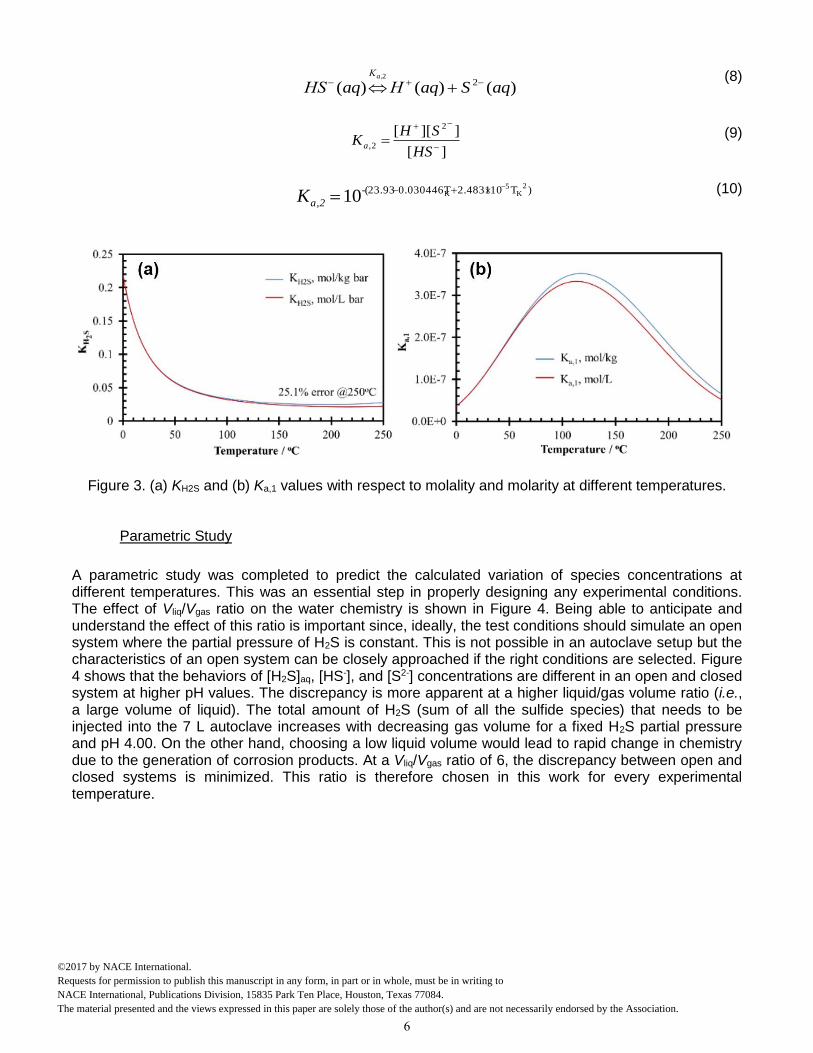
used in this model because of its widespread adoption, e.g, in the International Temperature Scale (ITS). The the equilibrium constants KH2S, Ka,1 and Ka,2 calculated based on the research described by Suleimenov20,21 and Ning22 (Equations (2)-(10)), but modified from molality to molarity units. Originally, these values were as molality units (mol/kg bar), but were here used in molarity (mol/L bar) since the

numerical values are very close at temperatures under 100C.7,22 However, as shown in Figure 3, when used at higher temperature (typically above 100oC), large differences can appear (for example, more

than 25% error is apparent at 250C).

S(aq)ΗS(g)ΗSΗΚ

22

2

(2)

SH

SHp

SHK

2

2

][ 2 (3)

)log9.261/1671900011132.02709.027.346(

2

10 KKKK

2

TTTT

SHK

(4)

)()()(1

2 aqΗSaqΗaqSΗa,Κ

(5)

][

]][[

2

1,SH

HSHKa

(6)

KK

2K

4K 2ln142.741722/20565.7315101.67220.361261782.43945

1, 10TTTT

aK

(7)

5


)()()( 22

aqSaqΗaqΗSa,Κ

(8)

][

]][[ 2

2,

HS

SHKa

(9)

)T102.48310.030446T-(23.93

2K

5K10

a,2K

(10)

Figure 3. (a) KH2S and (b) Ka,1 values with respect to molality and molarity at different temperatures.

Parametric Study

A parametric study was completed to predict the calculated variation of species concentrations at different temperatures. This was an essential step in properly designing any experimental conditions. The effect of Vliq/Vgas ratio on the water chemistry is shown in Figure 4. Being able to anticipate and understand the effect of this ratio is important since, ideally, the test conditions should simulate an open system where the partial pressure of H2S is constant. This is not possible in an autoclave setup but the characteristics of an open system can be closely approached if the right conditions are selected. Figure 4 shows that the behaviors of [H2S]aq, [HS-], and [S2-] concentrations are different in an open and closed system at higher pH values. The discrepancy is more apparent at a higher liquid/gas volume ratio (i.e., a large volume of liquid). The total amount of H2S (sum of all the sulfide species) that needs to be injected into the 7 L autoclave increases with decreasing gas volume for a fixed H2S partial pressure and pH 4.00. On the other hand, choosing a low liquid volume would lead to rapid change in chemistry due to the generation of corrosion products. At a Vliq/Vgas ratio of 6, the discrepancy between open and closed systems is minimized. This ratio is therefore chosen in this work for every experimental temperature.

6


Figure 4. (a) Effect of Vliq/Vgas ratio on the concentrations of sulfur species, and (b) the total amount of

H2S in a 7 L autoclave at pH 4.00, T=25oC, pH2S=0.10 bar. The effect of temperature on the concentrations of sulfide species at a fixed pH 4.00 and 0.10 bar pressure of H2S is shown in Figure 5(a). All the species concentrations significantly vary with increasing temperature. However, what really matters for corrosion is not pH2S, but the concentration of dissolved H2S in the solution, [H2S]aq. In this work, [H2S]aq was kept at 0.00385 mol/L for every temperature to enable better comparisons. This corresponds to 0.10 bar H2S at 80oC. In order to maintain [H2S]aq as a constant at higher temperatures, the pH2S needs to be increased (Figure 5(b)). H2S corrosion at 80oC, 120oC, 160oC, and 200oC at a constant [H2S]aq will be investigated in this work.

Figure 5. Effect of temperature on concentrations of sulfur species at (a) constant pH2S=0.10 bar and

(b) constant [H2S]aq=0.00385 mol/L (pH2S=0.10 bar@80oC), pH=4.00.

Experimentally, the water chemistry at high temperature should be monitored and compared with theoretical values. However, due to the lack of a reliable reference electrode in high temperature and high pressure H2S environments, pH could not be measured in situ. Therefore, the water chemistry verification could not be directly done, but had to be back-calculated by characterization of liquid samples taken at the end of each experiment. Effect of High Temperature on H2S Corrosion Experiments based on the test matrix in Table 2 were performed to identify the effect of high temperature on the kinetics of corrosion and layer formation on mild steel in sour environments. The results are presented below.

7


Corrosion Rates

Figure 6 shows the corrosion rates over time at 80C, 120C, 160C, and 200C as measured by LPR. It can be seen that the initial corrosion rates increased with increasing temperature, and then quickly decreased to stable corrosion rates of 4.1, 3.8, 1.8 and 2.5 mm/y, respectively, from lowest to highest temperature. Overall, the steady-state corrosion rate decreased with temperature except at 200oC.

Figure 6. Corrosion rate at different temperatures from LPR measurement, [H2S]aq=0.00385 mol/L,

pH=4.00, 4 days, B=23 mV/decade.

The time-averaged corrosion rates obtained from weight loss are shown in Figure 7. They are in good agreement with the time-integrated corrosion rate from LPR using a B value of 23 mV/decade.

Figure 7. Comparison of corrosion rates between LPR and weight loss, [H2S]aq=0.00385 mol/L,

pH=4.00, 4 days, B=23 mV/decade.

8


Corrosion Products

The corrosion products on the steel surface were characterized by XRD as shown in Figure 8. While

mackinawite (FeS) was the main corrosion product detected at 80C, troilite (FeS), pyrrhotite (Fe1-xS, x=0~0.17) and pyrrhotite/pyrite (FeS2) became the dominant species as temperature was increased. With increasing temperature, the corrosion product became richer in sulfur; this is an indication of enhanced reaction kinetics for phase transformations. The morphologies of the formed corrosion products were also characterized by SEM, as shown in

Figure 9 and Figure 10. The SEM for the 80C specimen shows a mackinawite layer of 15 µm thickness, which is much thinner than the corresponding metal loss thickness calculated to be 42 µm. From the EDS line scan, the outer layer was identified to be likely an iron sulfide but an inner layer,

which consisted mostly of iron and oxygen was probably an iron oxide. At 120C, the SEM shows

troilite-like crystals on the surface and a much thicker layer (61~73 µm). The -Fe peaks are absent in the XRD pattern as the corrosion product is so thick, preventing the X-rays from reaching the metal

substrate. At 160C, pyrrhotite crystals were clearly observed. The thickness of the layer was only

about 10 µm, but still no -Fe peaks were detected by XRD, indicating the corrosion product layer was

very dense and compact. This is also probably why the corrosion rate at 160C was the lowest. The

corrosion products changed to planar flaky crystals at 200C. All the cross-sections show a two-layer structure at every temperature tested: an inner layer comprised of an iron oxide and an outer layer comprised of an iron sulfide. However, the iron oxide was not detected by XRD due to the top layer being too thick and compact for XRD penetration.

Figure 8. XRD patterns of corrosion products on the steel surface at different temperatures,

[H2S]aq=0.00385 mol/L, pH=4.00, 4 days.

9


Figure 9. SEM of morphologies and cross-sections at 80C (left) and 120oC (right), [H2S]aq=0.00385 mol/L, pH=4.00, 4 days.

10


Figure 10. SEM of morphologies and cross-sections at 160C (left) and 200C (right), [H2S]aq=0.00385 mol/L, pH=4.00, 4 days.

Surface Profilometry

After removal of the corrosion products using Clarke solution,23 the metal surface was characterized by profilometry, as shown in Figure 11 and Figure 12. No obvious localized corrosion was observed at

80C and 120C. The surface was relatively smooth and the corrosion could be considered as uniform.

However, at 160C some small pits could be observed with around a 1.2 pitting ratio (ratio of maximum pit rate to general corrosion rate) and 1.5 mm/y pit penetration rate. This can be treated only as

localized corrosion initiation. At 200C, many large pits appeared with a 3.2 pitting ratio and 8.2 mm/y pit penetration rate. The pitting ratio is not accurate since the pitting corrosion overwhelmed the whole general corrosion. Due to severe localized corrosion at this temperature, the stable LPR corrosion rate

11


was a little higher than at 160C (Figure 6). These results fit with Ning’s previous work24 where it was found that once there is pyrite formation, localized attack would occur.

Figure 11. Surface profilometry after removing corrosion products at 80C (left) and 120C (right),

[H2S]aq=0.00385 mol/L, pH=4.00, 4 days.

Figure 12. Surface profilometry after removing corrosion products at 160oC (left) and 200oC (right),

[H2S]aq=0.00385 mol/L, pH=4.00, 4 days.

12


DISCUSSION

The current results are insufficient to make conclusive mechanistic statements, however, there are some new findings that are worthy of a discussion, especially in the context of the existing literature.

Formation of Iron Oxide

Iron oxide was found, at every temperature tested, as the main component of the inner corrosion product layer (Figure 9 and Figure 10). Until now, iron oxide has not been given much attention as a corrosion product in H2S corrosion environments. It is hypothesized that this iron oxide is magnetite (Fe3O4) due to the following observations:

Two Fe3O4 peaks were observed from XRD analysis at 80C (Figure 8), though they were not detected at other temperatures due to the top layer being either too thick or too compact for X-ray penetration;

Fe3O4 was also confirmed as an inner layer from a previous study in sour environments at 220oC;10

Fe3O4 is also the main corrosion product at high temperatures in CO2 environments.16 The kinetics of Fe3O4 formation is very fast, making the scaling tendency (ST that is the ratio of precipitation rate to corrosion rate) very high at high temperature. Fe3O4 can form on the metal surface according to reaction (11):

eaqHsOFelOHaqFe 2)(8)()(4)(3 432

2 (11)

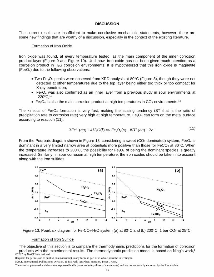
From the Pourbaix diagram shown in Figure 13, considering a sweet (CO2 dominated) system, Fe3O4 is

dominant in a very limited narrow area at potentials more positive than those for FeCO3 at 80C. When

the temperature increases to 200C, the possibility for Fe3O4 of being the dominant species is greatly increased. Similarly, in sour corrosion at high temperature, the iron oxides should be taken into account, along with the iron sulfides.

Figure 13. Pourbaix diagram for Fe-CO2-H2O system (a) at 80C and (b) 200C, 1 bar CO2 at 25C.

Formation of Iron Sulfide

The objective of this section is to compare the thermodynamic predictions for the formation of corrosion products with the experimental results. The thermodynamic prediction model is based on Ning’s work,8

13


which has not been verified above 80oC. In order to do so, a good understanding of the water chemistry at operating conditions needed to be developed. Since no direct measurement of pH and Fe2+ concentration could be performed in situ, some assumptions are needed as described below. The H2S concentration and Fe2+ concentration were measured using GC and spectrophotometry,

respectively, after cooling down the autoclave (usually to around 50C). The water chemistry was calculated at this measured temperature according to Equations (3), (6), (9), (13), and (15):

)()()(2 aqOHaqΗlOΗwΚ

(12)

]][[ OHΗKw (13)

)1047881.70737549.03868.29( 25

10 KK TT

wK

(14)

][][2][][][][2][ 22 OHSHSClHFeNa (15)

In Equation (15), for determining electroneutrality, the [Cl] is known experimentally by recording how

much NaCl and HCl (for pH adjustment) were added. There are 5 equations and 5 unknowns ([H2S],

[HS], [S2], [H+], and [OH]). The total amount of sulfur species was calculated by applying a molar balance:

constantSHSSHSHS aqaqaqg ][][][][ 2

22 (16)

It is assumed that no significant gain or loss of Fe2+ occurred during the test “cooling down” procedure, either by FeS precipitation or dissolution. The [Fe2+] concentration measured at the sampling temperature was assumed to be the same as under operating conditions. At the experimental temperature pH2S is also unknown, in addition to the 5 unknowns mentioned above, but the extra equation (16) can be used. The calculation results are summarized in Table 4.

Table 4. Summary of initial conditions and theoretical calculated final conditions.

Initial Conditions Final Conditions

T, oC pH2S, bar pH pH2S, bar pH Fe2+, ppm

80 0.10 4.00 0.07 5.47 1.79

120 0.14 4.00 0.11 5.42 5.82

160 0.14 4.00 0.14 5.48 4.26

200 0.18 4.00 0.16 5.78 2.31

Compared with the initial conditions, the final pH values all drifted from 4.00 to above 5.40, which represent conditions increasingly favorable for iron sulfide formation. These parameters are used to generate Pourbaix diagrams as shown in Figure 14. The red arrow represents the pH shifting and the likely potential range (around -500 mV vs. SHE). The Pourbaix diagrams provide useful information to understand the experimental results. Different polymorphs and related phases of iron sulfides were identified at the different temperatures tested. Fe3O4 and mackinawite were always observed after short exposure times, inferring that they always formed first. However, according to the Pourbaix diagrams in H2S environments, pyrite and pyrrhotite should be more stable than iron oxides and mackinawite, which act as precursors for the transformation

reactions.25 However, pyrrhotite and pyrite were only observed at 160C and 200C. This could be explained considering that the transformation kinetics are accelerated at higher temperatures.

Particularly at 200C, the “pH shift” arrow crosses the equilibrium line between pyrrhotite and pyrite,

14


indicating a possible iron sulfide transformation between pyrrhotite and pyrite, which is in good agreement with the XRD data (Figure 8).

Figure 14. Pourbaix diagram for Fe-H2S-H2O system, (a) 80C, mackinawite, (b) 120C, pyrrhotite

(troilite), (c) 160C, pyrrhotite, and (d) 200C, pyrite/pyrrhotite, other input parameters are in Table 4.

CONCLUSIONS

A water chemistry model for a closed system containing H2S was developed and checked for validity at high temperatures.

Sour corrosion experiments were conducted successfully at 80C, 120C, 160C and 200C. Initial corrosion rates increased with increasing temperature. Final corrosion rates, after 4 days of exposure, remained high at between 2 and 4 mm/y.

Iron sulfide transformation was observed for the first time in high temperature H2S corrosion. The inner corrosion product was iron oxide (postulated to be Fe3O4), the outer layer was mainly mackinawite, troilite, pyrrhotite and pyrite at 80oC, 120oC, 160oC and 200oC, respectively.

ACKNOWLEDGEMENTS

The authors would like to express sincere appreciation to the following industrial sponsors for their financial support and direction: Anadarko, Baker Hughes, BP, Chevron, China National Offshore Oil Corporation, ConocoPhillips, DNV GL, ExxonMobil, M-I SWACO, Occidental Oil Company, Petroleum Institute, PTT, Saudi Aramco, Shell Global Solutions, SINOPEC, TOTAL, TransCanada, WGK.

15


REFERENCES

1. G. DeBruijin, “High-pressure, high-temperature technologies,” Oilfield Review 20, 3(2008): p. 46-60. 2. H.J. Chen, “High temperature corrosion inhibition performance of imidazoline and amide,” CORROSION/2010, paper no. 00035 (San Antonio, TX: NACE, 2010). 3. S.S. Prabha, “Corrosion problems in petroleum industry,” European Chemical Bulletin 3, 3 (2014): p. 300-307. 4. H. Ma, X. Cheng, G. Li, S. Chen, Z. Quan, S. Zhao, L. Niu, “The influence of hydrogen sulfide on corrosion of iron under different conditions,” Corrosion Science 42, 10 (2000): p. 1669-1683. 5. W. Sun, S. Nesic, S. Papavinasam, "Kinetics of iron sulfide and mixed iron sulfide/carbonate scale precipitation in CO2/H2S corrosion," CORROSION/2006, paper no. 06644 (San Diego, CA: NACE, 2006). 6. J. Tang, Y. Shao, J. Guo, T. Zhang, G. Meng, F. Wang, "The effect of H2S concentration on the corrosion behavior of carbon steel at 90oC." Corrosion Science 52, 6 (2010): p. 2050-2058. 7. Y. Zheng, B. Brown, S. Nesic, “Electrochemical study and modeling of H2S corrosion of mild steel,” Corrosion, 70, 4 (2013): p. 351-365. 8. J. Ning, Y. Zheng, B. Brown, D. Young, and S. Nesic, “A Thermodynamic Model for the Prediction of Mild Steel Corrosion Products in an Aqueous Hydrogen Sulfide Environment,” Corrosion, 71, 8 (2015): p. 945-960. 9. W. Sun, D.V. Pugh, S.N. Smith, S. Ling, J.L. Pacheco, R.J. Franco, “A parametric study of sour corrosion of carbon steel,” CORROSION/2010, paper no. 10278 (San Antonio, TX: NACE, 2010). 10. T.A. Ramanarayanam, S.N. Smith, “Corrosion of Iron in Gaseous Environments and in Gas-Saturated Aqueous Environments,” Corrosion, 46, 1 (1990): p. 66-74. 11. F. Shi, L. Zhang, J. Yang, M. Lu, J. Ding, H. Li, “Polymorphous FeS corrosion products of pipeline steel under highly sour conditions,” Corrosion Science 102, (2016): p. 103-113. 12. E.B. Backensto, R.D. Drew, C.C. Stapleford, “High Temperature Hydrogen Sulfide Corrosion,” Corrosion, 12, 1 (1956): p. 22-32. 13. A.V. Skalunov, G.V. Sretenskaya, G.A. Tsarkov, “Effect of hydrogen sulfide and temperature on the corrosion behavior of high-alloy metals in precipitation baths for viscose manufacture,” Fibre Chemistry 18, 4 (1987): p. 321-325. 14. Y. Qi, H. Luo, S. Zheng, C. Chen, Z. Lv, M. Xiong, “Effect of Temperature on the Corrosion Behavior of Carbon Steel in Hydrogen Sulphide Environments,” International Journal of Electrochemical Science 9, (2014): p. 2101-2112. 15. Y. Zheng, J. Ning, B. Brown, S. Nesic, “Advancement in Predictive Modeling of Mild Steel Corrosion in CO2-and H2S-Containing Environments,” Corrosion 72, 5 (2016): p. 679-691. 16. T. Tanupabrungsun, D. Young, B. Brown, S. Nesic, “Construction and Verification of Pourbaix Diagrams for CO2 Corrosion of Mild Steel Valid up to 250°C,” CORROSION/2012, paper no. 0001418 (Salt Lake City, UT: NACE, 2012). 17. R. Thodla, F. Gui, K. Evans, C. Joia, I. P. Baptista, “Corrosion Fatigue Performance of Super 13 CR, Duplex 2205 and 2507 for Riser Applications,” CORROSION/2010, paper no. 10312 (San Antonio, TX: NACE, 2010). 18. J. Ning, Y. Zheng, B. Brown, D. Young, S. Nesic, “Construction and Verification of Pourbaix Diagrams for Hydrogen Sulfide Corrosion of Mild Steel,” CORROSION/2015, paper no. 5507 (Dallas, TX: NACE, 2015). 19. F.E. Jones, G.L. Harris, “ITS-90 density of water formulation for volumetric standards calibration,” Journal of research of the National Institute of Standards and Technology 97, (1992): p. 335-340. 20. O.M. Suleimenov, R.E. Krupp, “Solubility of hydrogen sulfide in pure water and in NaCl solutions, from 20 to 320°C and at saturation pressures,” Geochimica et Cosmochimica Acta 58, 11 (1994): p. 2433-2444. 21. O.M. Suleimenov, T.M. Seward, “A spectrophotometric study of hydrogen sulphide ionisation in aqueous solutions to 350°C,” Geochimica et Cosmochimica Acta 61, 24 (1997): p. 5187-5198. 22. J. Ning, Y. Zheng, D. Young, B. Brown, S. Nesic, “Thermodynamic Study of Hydrogen Sulfide Corrosion of Mild Steel,” Corrosion 70, 4 (2014): p. 375-389.

16


23. D.D.N. Singh, A. Kumar, “A Fresh Look at ASTM G 1-90 Solution Recommended for Cleaning of Corrosion Products Formed on Iron and Steels,” Corrosion 59, 11 (2003): p. 1029-1036. 24. J. Ning, Y. Zheng, B. Brown, D. Young, S. Nesic, “The Role of Iron Sulfide Polymorphism in Localized H2S Corrosion of Mild Steel,” CORROSION/2016, paper no. 7502 (Vancouver, BC: NACE, 2016). 25. L.G. Benning, R.T. Wilkin, H.L. Barnes, “Reaction pathways in the Fe-S system below 100oC,” Chemical Geology 167, 1 (2000): p. 25-51.

17


Documents

Paper No. 9084 - Institute for Corrosion and Multiphase ... · Linear polarization resistance (LPR) and weight loss ... The corrosion rate eventually reached a stable value due to