Embed Size (px)
Citation preview

Paper P052009
ANALYSIS OF METABOLIC DISORDER – GOUT MidWest SAS® Users Group (MWSUG)
Sireesha Ramoju, University of Louisville, Louisville KY
ABSTRACT
The purpose of this project is to examine the analysis of metabolic disorder called Gout. This disease is created by a buildup of uric acid crystals deposited on the articular cartilage joints, tendons and surrounding tissues. Medical treatment for gout usually involves Short‐term treatment and Long‐term treatment. Kernel Density Estimation is used to examine the ratio of the disease, medication and cost. The Logistic Regression and Linear Regression analysis are used to find the various demographic factors that affect the Gout disease. The data are from MEPS (http://www.meps.ahrq.gov). SAS software is used for the analysis of Kernel Density Estimation, Logistic Regression and Linear Regression. Finally the study shows that Gout is affecting men mostly in the age group of 40 – 70 and in women after menopause, majority of Gout affected patients are using Allopurinol as a long term treatment, and those who are diagnosed with digestive disorders will have more chances of having the gout disease.

INTRODUCTION
Gout is an ancient and common form of inflammatory arthritis, and is the most common inflammatory arthritis among men. Gout is a chronic disease caused by an uncontrolled metabolic disorder, hyperuricemia, which leads to the deposition of monosodium urate crystals in tissue. Hyperuricemia means too much uric acid in the blood. Uric acid is a metabolic product resulting from the metabolism of purines. When crystals form in the joints it causes recurring attacks of joint inflammation. Chronic gout can also lead to deposits of hard lumps of uric acid in and around the joints and may cause joint destruction and decreased kidney function. Gout has the unique distinction of being one of the most frequently recorded medical illnesses throughout history. It is often related to an inherited abnormality in the body's ability to process uric acid. Uric acid is a breakdown product of purines that are part of many foods we eat. An abnormality in handling uric acid can cause attacks of painful arthritis (gout attack), kidney stones, and blockage of the kidney‐filtering tubules with uric acid crystals. On the other hand, some people may only develop elevated blood uric acid levels without having arthritis or kidney problems. The term gout refers the disease that is caused by an overload of uric acid in the body, resulting in painful arthritic attacks and deposits of lumps of uric acid crystals in body tissues. Chronic gout is characterized by chronic arthritis, with soreness and aching of joints. People with gout may also get tophi (masses of urate crystals deposited in soft tissue)—usually in cooler areas of the body (e.g., elbows, ears, distal finger joints).
There are two key concepts essential to treating gout. First, it is critical to stop the acute inflammation of joints affected by gouty arthritis. Second, it is important to address the long‐term management of the disease in order to prevent future gouty arthritis attacks and shrink gouty tophi crystal deposits. Short‐term treatment, using medicines that relieve pain and reduce inflammation during an acute attack or prevent a recurrence of an acute attack. Colchicine, to prevent flare‐ups during the first months that you are taking uric acid‐lowering medicines. Long‐term treatment, using medicines to lower uric acid levels in the blood, which can reduce the frequency and severity of gout attacks in the future. Allopurinol, to decrease production of uric acid by the body. Information about the medications for Gout was obtained from the MedicineNet (http://www.medicinenet.com/gout/article.htm).
According to the study in a managed care population showed an increase in prevalence of gout from 2.9 to 5.2 per 1000 enrollees in the time period 1990 to 1999. For those under age 65, rates among men were 4 times those of women; over age 65 rates among men were 3 times greater. Most of the increase occurred among enrollees over the age of 65: among those over age 75, the prevalence increased (1990 to 1999) from 21 to 41 per 1000 enrollees. Among those 65 to 74, prevalence increased from 21 to 31 per 100 enrollees.
The data set is used for this analysis is prescription Medicine data of 2006 from the MEPS database. Data are extracted using ICD9 condition codes. Gout was defined by ICD‐9‐CM codes 274 or use of uric acid lowering drugs. Data has 341,994 records. The prescription data are missing patient demographic information, which are extracted from the population characteristics dataset by joining the 2 datasets using an unique identifier. Kernel Density is used to analyze the various factors those are affecting Gout disease. Logistic regression is conducted on the data to find whether there is any relationship between Gout and various digestive diseases which causes acidity in the bloodstreams. Linear Regression is used in the analysis to find whether age, sex and race of the patient are affecting the Gout disease. Patient records, which are having digestive diseases, are extracted from the data set using ICD‐9 codes between 520‐579.

METHOD The data source of the project is MEPS. The web site is http://www.meps.ahrq.gov/mepsweb/data_stats/download_data_files.jsp. The data files are directly downloaded from this website. The data are then extracted using SAS Enterprise Guide based on the ICD9 codes of Gout and various digestive diseases. ICD 9 code for Gout is 274. Patients’ information for various digestive diseases are extracted using ICD9 codes between 520‐579. For patient’s demographic information obtained the population characteristics 2006 data from the website http://www.meps.ahrq.gov/mepsweb/data_stats/download_data_files.jsp and joining this data with prescription data. To extract the Gout patients with Gastric problems, obtained Gout patients and Gastric patients separately and mergered these 2 datasets. This study will use Kernel Density Estimation, logistic and linear regression techniques to determine which factors to include; age, race, gender and Digestive diseases have the most significant influence on a Gout patient. SAS (Statistical Analysis Software) is used in this project. The SAS software provides extensive statistical capabilities, including tools for both specialized and enterprise‐wide analytical needs. The SAS System includes a wide range of statistical analyses, including analysis of variance, regression analysis, kernel density estimation, categorical data analysis, multivariate analysis, survival analysis, psychometric analysis, cluster analysis, and nonparametric analysis. SAS Enterprise Guide brings the power of the SAS System to the desktop in a thin‐client Windows application. For this project, SAS Enterprise Guide is used to do Kernel Density Estimation, Logistic Regression and Linear Regression.
Kernel Density Estimation:
In statistics, kernel density estimation is a non‐parametric way of estimating the probability density function of a random variable.If x1, x2, ..., xN ~ ƒ is an independent and identically‐distributed sample of a random variable, then the kernel density approximation of its probability density function is
where K is some kernel and h is a smoothing parameter called the bandwidth. Quite often K is taken to be a standard Gaussian function with mean zero and variance 1:
PROC KDE uses only the standard normal density for K but allows for several different methods to estimate the bandwidth, as discussed below. The default for the univaraiate smoothing is that of Sheather‐Jones plug in (SJPI).
Where c3 and c4 are appropriate functionals. The unknown values depending upon the density function f(X) are estimated with bandwidths chosen by reference to a parametric family such as the Gaussian as provided in Silverman:
However, the procedure uses a different estimator, the simple normal reference (SNR), as the default for the bivariate estimator:
Along with Silverman’s rule of thumb(SROT):

and the over‐smoothed method(OS):
Logistic Regression Logistic regression analysis (LRA) extends the techniques of multiple regression analysis to research situations in which the outcome variable is categorical. In practice, situations involving categorical outcomes are quite common. In the setting of evaluating an educational program, for example, predictions may be made for the dichotomous outcome of success/failure or improved/not‐improved. Similarly, in a medical setting, an outcome might be presence/absence of disease. The focus of this document is on situations in which the outcome variable is dichotomous, although extension of the techniques of LRA to outcomes with three or more categories (e.g., improved, same, or worse) is possible. In this section, we review the multiple regression model and then, present the model for LRA.
The standard procedure for Logistic Regression has been to use an equation of the form
Y= β0 + β1 X1 + … + βk Xk + e
Where Y= dependent variable.
X1, X2,...,Xk = independent variables,
e = random error, and
βi = determines the contribution of the independent variable Xi.
The variable Y should be discrete for logistic regression. Each X variable denotes the presence or absence of a factor for a particular observation.
Here, Y is a binary variable that contains a value of 0 or 1. The value of 0 represents the person diagnosed with Gout. And 1 represents the person not diagnosed with Gout.
For this analysis, there are 6 variables used for Logistic Regression.
The Logistic Regression equation can be written as
P = α0 + α1(Sex) + α2(Race) + α3(Age) + α4(Gastro_RXICD1X) + α5(Gastro_RXICD2X) + α6(Gastro_RXICD3X)
Linear Regression Linear regression analyzes the relationship between two variables, X and Y. For each subject (or experimental unit), both X and Y, find the best straight line through the data. In some situations, the slope and/or intercept have a scientific meaning. In other cases, use the linear regression line as a standard curve to find new values of X from Y, or Y from X. The general linear model is used to perform linear regression. Linear regression assumes that an interval(continuous) outcome variable is a linear relationship of a series of input variables. These input variables can be nominal, ordinal, or interval. For example, suppose we want to examine the relationship of teaching time to research time in the workload database.
The methodology looks very similar to that of logistic regression in that
Y = β0 + β1 X1+ β2 X2 +…..+ βn Xn

However, in this case, Y is assumed to be an interval or continuous variable. Again, X1, … Xn can be continuous ordinal , or nominal.
It must be assumed that there is an error term, εi, where εi is the difference between the actual value of Y and the predicted value of Y. Then we assume that the values of ε1, ε2,… εn are from a normal distribution(with a bell‐shaped density curve). Moreover, the average value of the ε1, ε2,…, εn must equal zero.
RESULTS We first examine patient demographic information Gender(frequency)
Fig 1.1 Fig 1.1 shows that the majority of those prescribed for Gout treatment are male (77%). This does not really mean that males are at more risk with Gout than women, but it does mean that the percentage of medical prescriptions is more for males than females. To analyze the data more statistically, we need to use Kernel Density Estimation. This is shown in Fig 1.2
proc kde data=SASUSER.SORTSEXGOUTWITHDEMO_2006 gridl=20 gridu=100 method=SJPI BWM=1 out=kdeagebysex; var AGE; by SEX; run;

Fig 1.2 1 – Men, 2 – Women Figure 1.2 gives the Kernel Density for Men and Women. For women, the high peak for prescriptions is around 65 to 70 years with another high peak for women around the age of 80 and 90. There is a big dip in the number of prescriptions for women around the age of 70. Also, another obvious observation is that women over the age of 60 have peaked 3 times, with the only exception a big dip around 70 that could possibly be due to a lack of prescription data. This verifies the general assumption that women peak in the prescriptions of medicine after the age of 60. The graph shows that during the lifetime of a patient with Gout, men have a high peak of prescription around 55 to 60 years of age. The beginning of prescription data for men is clearly over the age of 40. Finally, the Kernel Density Estimation shows that men have a high number of prescriptions at and above age 40; women have high peak at and above the age group of 60.

Summary of the prescription data according to the different races:
Category Race Number of Observations
1 Caucasian 863
2 African American 290
3 American Indian/Alaska Native 14
4 Asian 60
5 Native Hawaiian/Pacific Islander 6
6 Multiple Races reported 11
Table 1
Table 1 shows that the Category 1(Caucasian) has more prescription data records (863). Category 2 has 290 observations and category 4 has 60. As Categories 3, 5 and 6 have fewer observations, they are combined into the Other category. The below shown Fig 1.3 shows a pie‐chart based on these table data. Caucasians will have the most prescriptions since they have the most people.
Fig 1.3 Fig 1.3 shows the pie‐chart based on the different races. The percentages show that the number of observations for Prescription medicine data of Caucasian (category 1) is 69.37%. The percentage is 23.31% for African American, 4.82% is for

Asians and the Other category has 2.49%. Here, we are not comparing which category has more prescription medicine data. We are merely looking at the percentages of Prescription medicine data based on the available data. However, according to census information, Caucasians make up 77% of the population; African American comprises 13%. African Americans are more susceptible to gout compared to the other races.
Kernel Density Estimation code in SAS Enterprise Guide
proc kde data=SASUSER.SORTRaceGOUTWITHDEMO_2006 gridl=20 gridu=100 method=SNR out=kdeagebyrace; var AGE; by RACE; run;
Fig 1.4 ‐ Kernel Density Estimation for different Races in the MEPS data
1 – White 2 – Black 3 – American Indian/Alaska Native 4 – Asian 5 – Native Hawaiian/Pacific Islander 6 – Multiple Races reported Fig 1.4 shows a Kernel Density distribution for Gout patients of different races. The graph shows a high peak around 40 years of age for Asians. Similarly, the high peak for Native Hawiian/Pacific Islander is around 50 years of age, for Whites is around 80, for American Indian/Alaskan natives is around 55 years of age, and for Blacks is around 70 years of age.

According to the data statistics, it is found that there are two medications that are prescribed more for this disease. They are Allopurinol , which is used to prevent Gout, the other one is Colchicine which is used to reduce the inflammation of the patient’s affected body. Apart from these two, there are some other medicines such as Indocin, Indomethacin etc. The sample taken here consists of Allopurinol and Colchicine as they have more data available. The Kernel Density Estimation between these two medications is as shown below:
KDE by Medicine Type
proc kde data=SASUSER.SORTMEDTYPEAGERANGE_2006 gridl=20 gridu=100 method=OS BWM=0.8 out=kdeMEDTYPE; var AGE; by MEDICIN_TYPE; run;
Fig 1.5
0 ‐ Colchicine 1 – Allopurinol Fig 1.5 shows the Kernel Density Estimation for two medicine types. At around 55 years of age, 1‐ Allopurinol is used more, meaning that the patients are going for a cure. At around 80 years of age, both medications are used to prevent and cure the Gout disease. The density is somewhat uniformly distributed between the ages of 65 and 75 for both the medications. Also, there is a sudden spike at around 40 for Allopurinol users, which means that Gout begins in people around that age.

KDE by Medicine cost:
proc kde data=SASUSER.SORT_MED_TYPE_2006 gridl=0 gridu=200 method=SNR out=kdeTotal_COST; var RX_COST; by MEDICIN_TYPE; run;
Fig 1.6
Fig 1.6 shows the Kernel Density Estimation for Allopurinol and Colchicine on a cost based on the prescription purchase data available. According to the above estimate, the cost of Allopurinol usage is relatively higher than that for Colchicine.
Logistic Regression Results
For Logistic Regression the responsible variable is having Gout. A value of 0 means the person has gout and a value of 1 means the person does not have gout. The Logistic regression model in the analysis of data defined using 16784 patients who are prescribed with various digestive diseases. The data contain 7 types of major digestive diseases. In this data, 506 people got a prescription for Gout disease. The dependent variables for this analysis are RXICD1X, RXICD2X AND RXICD3X. All parameters were codified as binary variables; the value '0' is with Gout and '1' is without Gout. The purpose of this analysis is to identify from the 7 diagnostics, the one that is most relevant one and to find out whether there is a significant impact on having Gout or not.

ICD9 codes DISEASES OF THE DIGESTIVE SYSTEM (520‐579)
Other Other diseases
520‐529 DISEASES OF ORAL CAVITY, SALIVARY GLANDS, AND JAWS
530‐538 DISEASES OF ESOPHAGUS, STOMACH, AND DUODENUM
540‐543 APPENDICITIS
550‐553 HERNIA OF ABDOMINAL CAVITY
555‐558 NONINFECTIOUS ENTERITIS AND COLITIS
560‐569 OTHER DISEASES OF INTESTINES AND PERITONEUM
570‐579 OTHER DISEASES OF DIGESTIVE SYSTEM
Table 1.1 Digestive System Diseases
The above table 1.1 describes the top 7 diseases of digestive system and their ICD9 codes.
Category ICD9 codes Number of
Observations having Gout
Number of
Observations not having Gout
Total
0 Other 11 534 385
1 520‐529 23 1398 1421
2 530‐538 402 10996 11398
3 540-543 0 21 21
4 550‐553 13 521 534
5 555-558 1 771 772
6 560-569 42 1601 1643
7 570-579 14 596 610
Total 506 16278 16784
Table 1.2 Frequency counts
The above table 1.2 describes the frequency counts of various digestive diseases.

Category Sex Number of
Observations having Gout
Number of
Observations not having Gout
Total
1 Male 953 129760 130713
2 Female 291 210990 211281
Total 1244 340750 341994
Category Race Number of
Observations having Gout
Number of
Observations not having Gout
Total
1 Caucasian 863 266096 266959
2 African American 290 57500 57790
3 American Indian/Alaska Native 14 3152 3166
4 Asian 60 7269 7329
5 Native
Hawaiian/Pacific Islander
6 766 772
6 Multiple Races reported 11 5967 5978
Total 1244 340750 341994
Category Age range Number of
Observations having Gout
Number of
Observations not having Gout
Total
‐1 0‐19 11 29363 29363
0 20‐39 78 37030 37030
1 40-59 430 127334 127334
2 60‐79 581 11608 116008
3 Above 80 144 32259 32259
Total 1244 340750 341994
Table 1.3 Summary of the prescription data
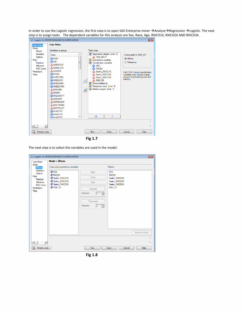
In order to use the Logistic regression, the first step is to open SAS Enterprise miner Analyze Regression Logistic. The next step is to assign tasks. The dependent variables for this analysis are Sex, Race, Age, RXICD1X, RXICD2X AND RXICD3X.
Fig 1.7
The next step is to select the variables are used in the model:
Fig 1.8

The final step is to select the ROC curve:
Fig 1.9
The results of the Logistic regression are as follows:
Table of Gastro_RXICD1X by HAS_GOUT
HAS_GOUT Gastro_RXICD1X
0 1
Total
0 11 2.86 2.17
374 97.14 2.30
385
1 23 1.62 4.55
1398 98.38 8.59
1421
2 402 3.53 79.45
10996 96.47 67.55
11398
3 0
0.00 0.00
21 100.00 0.13
21
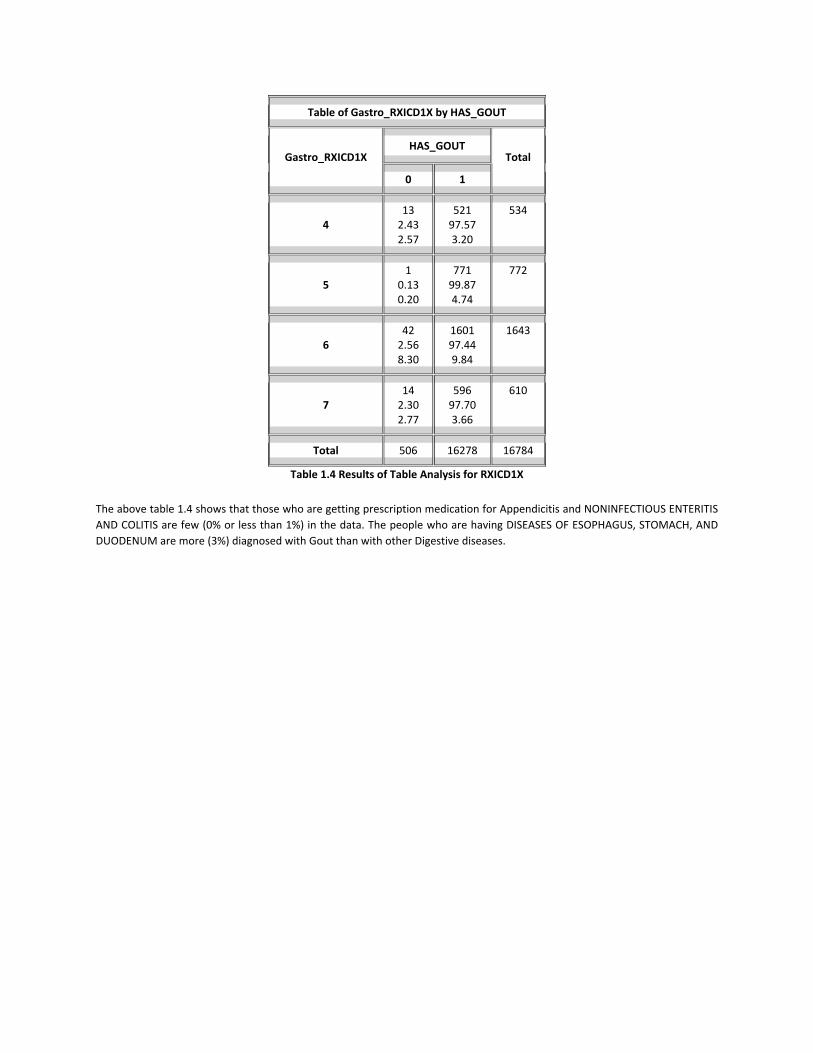
Table of Gastro_RXICD1X by HAS_GOUT
HAS_GOUT Gastro_RXICD1X
0 1
Total
4 13 2.43 2.57
521 97.57 3.20
534
5 1
0.13 0.20
771 99.87 4.74
772
6 42 2.56 8.30
1601 97.44 9.84
1643
7 14 2.30 2.77
596 97.70 3.66
610
Total 506 16278 16784
Table 1.4 Results of Table Analysis for RXICD1X
The above table 1.4 shows that those who are getting prescription medication for Appendicitis and NONINFECTIOUS ENTERITIS AND COLITIS are few (0% or less than 1%) in the data. The people who are having DISEASES OF ESOPHAGUS, STOMACH, AND DUODENUM are more (3%) diagnosed with Gout than with other Digestive diseases.

Table of Gastro_RXICD2X by HAS_GOUT
HAS_GOUT Gastro_RXICD2X
0 1
Total
0 4933.0597.43
1566296.9596.22
16155
1 68.961.19
6191.040.37
67
2 41.320.79
30098.681.84
304
3 00.000.00
6100.000.04
6
4 00.000.00
30100.000.18
30
6 00.000.00
135100.000.83
135
7 33.450.59
8496.550.52
87
Total 506 16278 16784
Table 1.5 Results of Table Analysis for RXICD2X
The above table 1.5 shows that those who are getting prescription medication for type 3, 4, 5 are very unlikely (0% or less than 1%) in the data. The people who have type 1 diseases are more likely (3%) to be diagnosed with Gout than with other Digestive diseases.

Table of Gastro_RXICD3X by HAS_GOUT
HAS_GOUT Gastro_RXICD3X
0 1
Total
0 5063.03
100.00
1617896.9799.39
16684
1 00.000.00
14100.000.09
14
2 00.000.00
51100.000.31
51
4 00.000.00
5100.000.03
5
6 00.000.00
12100.000.07
12
7 00.000.00
18100.000.11
18
Total 506 16278 16784
Table 1.5 Results of Table Analysis for RXICD3X
The above table 1.5 shows that none of those diagnosed for type1, 2, 3, 4, 5, 6, 7 have Gout in the data. We now perform a Logistic Regression with outcome variables Ages, Sex, Race, Gastro_RXICD1X, Gastro_RXICD2X and Gastro_RXICD3X.
Testing Global Null Hypothesis: BETA=0
Test Chi-Square DF Pr > ChiSq
Likelihood Ratio 193.8311 28 <.0001
Score 180.3019 28 <.0001
Wald 144.0170 28 <.0001
Table 1.6 Chi Square Test of Hypothesis The above table 1.6 shows the probability of being wrong when rejecting H0.

Type 3 Analysis of Effects
Effect DF WaldChi-Square
Pr > ChiSq
SEX 1 36.6604 <.0001
RACEX 5 35.4376 <.0001
Gastro_RXICD1X 7 21.4819 0.0031
Gastro_RXICD2X 6 8.9288 0.1776
Gastro_RXICD3X 5 0.0031 1.0000
AGE_CD 4 35.4558 <.0001
Table 1.7 Chi Square Test for each X‐Variable The above table 1.7 shows that the first diagnosis codes and demographics are statistically significant on the model.
Analysis of Maximum Likelihood Estimates
Parameter DF Estimate StandardError
WaldChi-Square
Pr > ChiSq
Intercept 1 -23.1028 310.1 0.0055 0.9406
SEX 1 1 0.2797 0.0462 36.6604 <.0001
RACEX 1 1 1.8767 77.4954 0.0006 0.9807
RACEX 2 1 1.9048 77.4954 0.0006 0.9804
RACEX 3 1 0.4836 77.4997 0.0000 0.9950
RACEX 4 1 3.0893 77.4955 0.0016 0.9682
RACEX 5 1 -9.6334 387.5 0.0006 0.9802
Gastro_RXICD1X 0 1 2.6666 58.2547 0.0021 0.9635
Gastro_RXICD1X 1 1 1.3284 58.2502 0.0005 0.9818
Gastro_RXICD1X 2 1 1.9776 58.2499 0.0012 0.9729
Gastro_RXICD1X 3 1 -9.9942 407.7 0.0006 0.9804
Gastro_RXICD1X 4 1 1.7142 58.2504 0.0009 0.9765
Gastro_RXICD1X 5 1 -1.2060 58.2563 0.0004 0.9835
Gastro_RXICD1X 6 1 1.7472 58.2501 0.0009 0.9761
Gastro_RXICD2X 0 1 5.5450 150.8 0.0014 0.9707

Analysis of Maximum Likelihood Estimates
Parameter DF Estimate StandardError
WaldChi-Square
Pr > ChiSq
Gastro_RXICD2X 1 1 6.2947 150.8 0.0017 0.9667
Gastro_RXICD2X 2 1 4.3486 150.8 0.0008 0.9770
Gastro_RXICD2X 3 1 -8.0259 822.8 0.0001 0.9922
Gastro_RXICD2X 4 1 -6.8525 375.9 0.0003 0.9855
Gastro_RXICD2X 6 1 -6.4874 213.9 0.0009 0.9758
Gastro_RXICD3X 0 1 10.3263 253.1 0.0017 0.9675
Gastro_RXICD3X 1 1 -2.1126 567.9 0.0000 0.9970
Gastro_RXICD3X 2 1 -1.5176 344.2 0.0000 0.9965
Gastro_RXICD3X 4 1 -2.7653 892.7 0.0000 0.9975
Gastro_RXICD3X 6 1 -2.1411 596.8 0.0000 0.9971
AGE_CD -1 1 -0.0194 0.1718 0.0127 0.9102
AGE_CD 0 1 -0.5273 0.1536 11.7813 0.0006
AGE_CD 1 1 -0.1631 0.0887 3.3805 0.0660
AGE_CD 2 1 0.2499 0.0851 8.6155 0.0033
Table 1.8 Analysis of Maximum Likelihood Estimates
Odds Ratio Estimates
Effect Point Estimate 95% Wald Confidence Limits
SEX 1 vs 2 1.749 1.460 2.097
RACEX 1 vs 6 0.669 0.382 1.171
RACEX 2 vs 6 0.688 0.377 1.256
RACEX 3 vs 6 0.166 0.021 1.287
RACEX 4 vs 6 2.249 1.127 4.485
RACEX 5 vs 6 <0.001 <0.001 >999.999
Gastro_RXICD1X 0 vs 7 2.461 0.422 14.357

Odds Ratio Estimates
Effect Point Estimate 95% Wald Confidence Limits
Gastro_RXICD1X 1 vs 7 0.646 0.328 1.272
Gastro_RXICD1X 2 vs 7 1.235 0.718 2.126
Gastro_RXICD1X 3 vs 7 <0.001 <0.001 >999.999
Gastro_RXICD1X 4 vs 7 0.949 0.441 2.044
Gastro_RXICD1X 5 vs 7 0.051 0.007 0.391
Gastro_RXICD1X 6 vs 7 0.981 0.530 1.818
Gastro_RXICD2X 0 vs 7 1.444 0.190 10.988
Gastro_RXICD2X 1 vs 7 3.056 0.709 13.169
Gastro_RXICD2X 2 vs 7 0.437 0.083 2.291
Gastro_RXICD2X 3 vs 7 <0.001 <0.001 >999.999
Gastro_RXICD2X 4 vs 7 <0.001 <0.001 >999.999
Gastro_RXICD2X 6 vs 7 <0.001 <0.001 >999.999
Gastro_RXICD3X 0 vs 7 >999.999 <0.001 >999.999
Gastro_RXICD3X 1 vs 7 0.724 <0.001 >999.999
Gastro_RXICD3X 2 vs 7 1.313 <0.001 >999.999
Gastro_RXICD3X 4 vs 7 0.377 <0.001 >999.999
Gastro_RXICD3X 6 vs 7 0.704 <0.001 >999.999
AGE_CD ‐1 vs 3 0.619 0.385 0.995
AGE_CD 0 vs 3 0.373 0.242 0.574
AGE_CD 1 vs 3 0.536 0.402 0.716
AGE_CD 2 vs 3 0.811 0.612 1.075
Table 1.9 Odds Ratio Estimates
The above table 1.9 Odds Ratios Estimates shows that all the diagnostic codes are statistically significant for having Gout disease. The first 7 comparisons show that increasing the X‐value from 1 to 7 will impact the chances of having Gout. Even though there are many other digestive diseases with Type 0 category, increasing the value of Y, the comparison of 3 to 7 will

decrease the value of Y. Those who are diagnosed with ESOPHAGUS, STOMACH, AND DUODENUM diseases will have more chances of having Gout disease. The above odds ratio estimates table shows that men are having double chances more than women who have Gout. The analysis also shows that as age increases chances of having gout will also increase. Even race also affects the chances of having Gout.
Association of Predicted Probabilities and ObservedResponses
Percent Concordant 63.2 Somers' D 0.339
Percent Discordant 29.4 Gamma 0.366
Percent Tied 7.4 Tau‐a 0.020
Pairs 8236668 c 0.669
Table 1.10 The above table 1.10 shows 63% accuracy of the model. It indicates that the model predicts the value of Y is half of the observations.

ROC Curve
Fig 1.10 ROC Curve
The graph above in Fig 1.7 shows the ROC curve between Sensitivity against Specificity. The area under the ROC curve is close to 1. It shows that the model is accurate.
The Linear regression model in the analysis of data is defined using 506 patients who are prescribed with gout and also prescribed with various digestive diseases. The data contains 7 types of major digestive diseases. The dependent variables for this analysis are 7 digestive diseases. The purpose of this analysis is to identify the relationship between these 7 diagnostics with Gout disease and demographics.

ICD9 codes DISEASES OF THE DIGESTIVE SYSTEM (520‐579)
Other Other diseases
520‐529 DISEASES OF ORAL CAVITY, SALIVARY GLANDS, AND JAWS
530‐538 DISEASES OF ESOPHAGUS, STOMACH, AND DUODENUM
540‐543 APPENDICITIS
550‐553 HERNIA OF ABDOMINAL CAVITY
555‐558 NONINFECTIOUS ENTERITIS AND COLITIS
560‐569 OTHER DISEASES OF INTESTINES AND PERITONEUM
570‐579 OTHER DISEASES OF DIGESTIVE SYSTEM
Table 1.11 Digestive System Diseases
The above table 1.11 describes the top 7 diseases of digestive system and their ICD9 codes.
Class Level Information
Class Levels Values SEX 2 1 2 RACEX 5 1 2 3 4 6
Table 1.12 Definition of class level variables The above table 1.12 represents all possible levels of the variables.
Number of Observations Read 506
Number of Observations Used 506
Table 1.13 Number of Observations Used in the model The above table 1.13 shows the number of observations in the dataset that do not contain missing values in either the input or outcome variables.
Source DF Sum of Squares Mean Square F Value Pr > F
Model 8 98.568050 12.321006 6.42 <.0001
Error 497 954.032741 1.919583
Corrected Total 505 1052.600791
Table 1.14 Overall Model Results

The above table 1.14 gives the overall results of the model. The p‐value is statistically significant (<0.000q), meaning that the input variables explain the variability in the outcome variables. It shows that the model is statistically significant.
R‐Square Coeff Var Root MSE Gastro_cd Mean
0.093642 56.81183 1.385490 2.438735
Table 1.15 R‐Square Value The above table 1.15 gives the percentage of variability in the outcome variables that can be explained by the input variables. Here 9% of the variability in the Research is explained by the variability in Age. The remaining 91% of the variability in the Research level is still not accounted for.
Source DF Type I SS Mean Square F Value Pr > F
AGE06X 1 9.80214398 9.80214398 5.11 0.0243
SEX 1 9.95905535 9.95905535 5.19 0.0232
RACEX 4 75.98466285 18.99616571 9.90 <.0001
SEX*RACEX 2 2.82218734 1.41109367 0.74 0.4800
Table 1.16 Type 1 sum of squares
Source DF Type III SS Mean Square F Value Pr > F
AGE06X 1 0.99284239 0.99284239 0.52 0.4724
SEX 1 8.64763603 8.64763603 4.50 0.0343
RACEX 4 70.80709599 17.70177400 9.22 <.0001
SEX*RACEX 2 2.82218734 1.41109367 0.74 0.4800
Table 1.17 Type 3 sum of squares As Sex*Race interaction is not significant in Type 1 SS and Type 3 SS, we can ignore the additional analysis on this variable. The rest of the variables are statistically significant on the model. So age, sex and race are statistically significant on Gout patients who are also getting prescription with various Gastro diseases.
Parameter Estimate Standard Error t Value Pr > |t|
Intercept 4.959917825 B 0.39127542 12.68 <.0001
AGE06X 0.002717612 0.00370827 0.73 0.4640
SEX 1 ‐0.385771641 B 0.12738698 ‐3.03 0.0026
SEX 2 0.000000000 B . . .
RACEX 1 ‐2.500118425 B 0.43567864 ‐5.74 <.0001

Parameter Estimate Standard Error t Value Pr > |t|
RACEX 2 ‐2.551500571 B 0.47088159 ‐5.42 <.0001
RACEX 3 ‐2.729050067 B 1.44940392 ‐1.88 0.0603
RACEX 4 ‐3.302865670 B 0.53062909 ‐6.22 <.0001
RACEX 6 0.000000000 B . . .
Table 1.18 Coefficients of Equation
H0:LSMean1=LSMean2 SEX Gastro_cd LSMEAN
Pr > |t|
1 2.51336894 0.0026
2 2.89914058
RACEX Gastro_cd LSMEAN LSMEAN Number
1 2.42284328 1
2 2.37146113 2
3 2.19391164 3
4 1.62009604 4
6 4.92296171 5
Table 1.19 Post‐Hoc Comparisons
Least Squares Means for effect RACEX Pr > |t| for H0: LSMean(i)=LSMean(j)
Dependent Variable: Gastro_cd
i/j 1 2 3 4 5
1 0.9986 0.9998 0.0410 <.0001
2 0.9986 0.9999 0.1334 <.0001
3 0.9998 0.9999 0.9943 0.3279
4 0.0410 0.1334 0.9943 <.0001
5 <.0001 <.0001 0.3279 <.0001
T able 1.20 P‐Value for Pair wise comparisons Tables 1.18 shows the pair wise comparisons between sex and race. Men are having more chances than women. And table 3.10 shows that race type 4 and 5 have more chances of having Gout with Gastric.

Figure 1.11 Relationship between actual and predicted values
The above figure 1.8 shows that the actual and predictions graph as scattered showing that some values are more difficult to predict compared to others.

Figure 1.12 Gastro with Gout versus Age
Figure 1.9 shows the relationship between Gout patients and age. It shows that the predicted model is more affective between the age of 40 and 80. Between 40 and 80 years of age, people will have more chances of having gout disease.
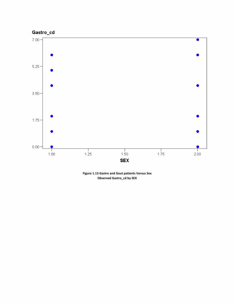
Figure 1.13 Gastro and Gout patients Versus Sex
Observed Gastro_cd by SEX

Figure 1.14 Gastro and Gout patients with Race Observed Gastro_cd by RACEX
As Sex and Race are class level variables, the above figures 1.10 and 1.11 show that sex and race are affecting Gout disease.
CONCLUSION This analysis concluded that the metabolic disorder, Gout, is highest in men around the age of 40 and highest in women around the age of 60. At the same time, the prescription medications used by the patients of this disorder are Allopurinol and Colchicine. Logistic regression technique is used to determine which factors to include; age, race, gender, Digestive disorders have the most significant influence on a patient having Gout disease. Results show that, for prescription medication patients a relationship exists between Digestive system diseases and Gout Disease. This analysis also concluded that those who are having ESOPHAGUS, STOMACH, AND DUODENUM diseases have more chances of getting Gout disease. Linear regression shows that Gout disease is linearly related to age. As age increases, chances of having Gout also increase. Finally, this analysis shows that age, sex and race are statistically significant on the model.

References 1. Cerrito PB. (2007). Statistical Data Analysis with Medical Data. Data Services Online, 1‐248. 2. US Department of Health & Human Services. Agency for Healthcare Research and Quality. Medical Expenditure Panel Survey. http://www.meps.ahrq.gov/mepsweb/data_stats/download_data_files.jsp3. Wikipedia, The free Encyclopedia. Gout. http://en.wikipedia.org/wiki/Gout4. Diseases and Injuries – Tabular List. http://icd9cm.chrisendres.com/icd9cm/index.php?action=alphaletter&letter=Go5. MedicineNet. “Diseases and Conditions”. http://www.medicinenet.com/gout/article.htm6. Gastric Problems. “Medication and Treatment.” Walsh’s Pharmacy Ltd http://www.pharmacy.on.ca/101/pharmacy/brochures3/gastric.htm7. Gout Medication http://www.webmd.com/a‐to‐z‐guides/gout‐medications
CONTACT INFORMATION
Your comments and questions are valued and encouraged. Contact the author at:
Name: Sireesha Ramoju Enterprise: University of Louisville E‐mail: [email protected]