Embed Size (px)
Citation preview
PARAMETER ESTIMATION FOR DYNAMICAL
SYSTEMS
by
Shelby R. Stanhope
B.S., Mathematics, Colorado State University, 2007
M.S., Mathematics, Colorado State University, 2010
Submitted to the Graduate Faculty of
the Kenneth P. Dietrich School of Arts and Sciences in partial
fulfillment
of the requirements for the degree of
Doctor of Philosophy
University of Pittsburgh
2016

UNIVERSITY OF PITTSBURGH
KENNETH P. DIETRICH SCHOOL OF ARTS AND SCIENCES
This dissertation was presented
by
Shelby R. Stanhope
It was defended on
June 20th 2016
and approved by
Dr. Jonathan Rubin, Professor, Department of Mathematics
Dr. David Swigon, Associate Professor, Department of Mathematics
Dr. Catalin Trenchea, Associate Professor, Department of Mathematics
Dr. Gilles Clermont, MD, Department of Critical Care Medicine UPMC
Dissertation Advisors: Dr. Jonathan Rubin, Professor, Department of Mathematics,
Dr. David Swigon, Associate Professor, Department of Mathematics
ii

Copyright c© by Shelby R. Stanhope
2016
iii

PARAMETER ESTIMATION FOR DYNAMICAL SYSTEMS
Shelby R. Stanhope, PhD
University of Pittsburgh, 2016
Parameter estimation is a vital component of model development. Making use of data, one
aims to determine the parameters for which the model behaves in the same way as the system
observations. In the setting of differential equation models, the available data often consists
of time course measurements of the system. We begin by examining the parameter estimation
problem in an idealized setting with complete knowledge of an entire single trajectory of data
which is free from error. This addresses the question of uniqueness of the parameters, i.e.
identifiability. We derive novel, interrelated conditions that are necessary and sufficient for
identifiability for linear and linear-in-parameters dynamical systems. One result provides
information about identifiability based solely on the geometric structure of an observed
trajectory. Then, we look at identifiability from a discrete collection of data points along
a trajectory. By considering data that are observed at equally spaced time intervals, we
define a matrix whose Jordan structure determines the identifiability. We further extend the
investigation to consider the case of uncertainty in the data. Our results establish regions in
data space that give inverse problem solutions with particular properties, such as uniqueness
or stability, and give bounds on the maximal allowable uncertainty in the data set that can be
tolerated while maintaining these characteristics. Finally, the practical problem of parameter
estimation from a collection of data for the system is addressed. In the setting of Bayesian
parameter inference, we aim to improve the accuracy of the Metropolis-Hastings algorithm
by introducing a new informative prior density called the Jacobian prior, which exploits
knowledge of the fixed model structure. Two approaches are developed to systematically
analyze the accuracy of the posterior density obtained using this prior.
iv

TABLE OF CONTENTS
PREFACE . . . . . . . . . . . . . . . . . . . . . . . . . . . . . . . . . . . . . . . . . xiv
1.0 INTRODUCTION . . . . . . . . . . . . . . . . . . . . . . . . . . . . . . . . . 1
2.0 IDENTIFIABILITY OF LINEAR AND LINEAR-IN-PARAMETERS
DYNAMICAL SYSTEMS FROM A SINGLE TRAJECTORY . . . . 8
2.1 Introduction . . . . . . . . . . . . . . . . . . . . . . . . . . . . . . . . . . . 8
2.2 Definitions and preliminaries . . . . . . . . . . . . . . . . . . . . . . . . . . 12
2.3 Identifiability conditions based on trajectory behavior or coefficient matrix
properties . . . . . . . . . . . . . . . . . . . . . . . . . . . . . . . . . . . . . 17
2.3.1 Analysis . . . . . . . . . . . . . . . . . . . . . . . . . . . . . . . . . . 17
2.3.2 Examples . . . . . . . . . . . . . . . . . . . . . . . . . . . . . . . . . 21
2.4 Partial identifiability from a confined trajectory . . . . . . . . . . . . . . . . 28
2.4.1 Analysis . . . . . . . . . . . . . . . . . . . . . . . . . . . . . . . . . . 28
2.4.2 Example . . . . . . . . . . . . . . . . . . . . . . . . . . . . . . . . . 30
2.5 Systems that are linear in parameters . . . . . . . . . . . . . . . . . . . . . 31
2.5.1 Analysis . . . . . . . . . . . . . . . . . . . . . . . . . . . . . . . . . . 31
2.5.2 Examples . . . . . . . . . . . . . . . . . . . . . . . . . . . . . . . . . 33
2.6 Discrete data . . . . . . . . . . . . . . . . . . . . . . . . . . . . . . . . . . . 35
2.7 Conclusions . . . . . . . . . . . . . . . . . . . . . . . . . . . . . . . . . . . . 39
3.0 ROBUSTNESS OF SOLUTIONS OF THE INVERSE PROBLEM FOR
LINEAR DYNAMICAL SYSTEMS WITH UNCERTAIN DATA . . . 41
3.1 Introduction . . . . . . . . . . . . . . . . . . . . . . . . . . . . . . . . . . . 41
3.2 Definitions and preliminaries . . . . . . . . . . . . . . . . . . . . . . . . . . 42
v

3.3 Existence and uniqueness of the inverse in n dimensions . . . . . . . . . . . 44
3.3.1 Inverse problems on open sets . . . . . . . . . . . . . . . . . . . . . . 44
3.3.2 Companion matrix formulation . . . . . . . . . . . . . . . . . . . . . 49
3.3.3 Examples . . . . . . . . . . . . . . . . . . . . . . . . . . . . . . . . . 50
3.4 Analysis of uncertainty in the determination and characterization of inverse 52
3.4.1 Analytical lower bound . . . . . . . . . . . . . . . . . . . . . . . . . 55
3.4.2 Analytical upper bound . . . . . . . . . . . . . . . . . . . . . . . . . 59
3.4.3 Numerical bound . . . . . . . . . . . . . . . . . . . . . . . . . . . . . 61
3.4.4 Analytical bounds for additional properties . . . . . . . . . . . . . . 61
3.5 Examples for two-dimensional systems . . . . . . . . . . . . . . . . . . . . . 63
3.5.1 Regions of existence and uniqueness of the inverse . . . . . . . . . . 63
3.5.2 Classifying the equilibrium point associated with the inverse . . . . . 66
3.5.3 Bounds on maximal permissible uncertainty . . . . . . . . . . . . . . 67
3.6 Remark on nonuniform spacing of data . . . . . . . . . . . . . . . . . . . . . 73
3.7 Discussion . . . . . . . . . . . . . . . . . . . . . . . . . . . . . . . . . . . . . 75
4.0 THE JACOBIAN PRIOR IMPROVES PARAMETER ESTIMATION
WITH THE METROPOLIS-HASTINGS ALGORITHM . . . . . . . . . 78
4.1 Introduction . . . . . . . . . . . . . . . . . . . . . . . . . . . . . . . . . . . 78
4.2 Preliminaries . . . . . . . . . . . . . . . . . . . . . . . . . . . . . . . . . . . 79
4.2.1 Model and notation . . . . . . . . . . . . . . . . . . . . . . . . . . . 79
4.2.2 Bayesian inference for parameter estimation . . . . . . . . . . . . . . 81
4.2.3 Metropolis-Hastings algorithm . . . . . . . . . . . . . . . . . . . . . 83
4.3 Theoretical derivation of the Jacobian prior . . . . . . . . . . . . . . . . . . 85
4.4 Systematic analysis of the influence of the prior . . . . . . . . . . . . . . . . 86
4.4.1 Linear systems . . . . . . . . . . . . . . . . . . . . . . . . . . . . . . 88
4.4.1.1 Comparison of priors: Approach 1 . . . . . . . . . . . . . . . 88
4.4.1.2 Notes on the implementation of Approach 1 and the Jacobian
prior in the Metropolis-Hastings algorithm . . . . . . . . . . 89
4.4.1.3 Approach 1 examples . . . . . . . . . . . . . . . . . . . . . . 91
4.4.1.4 Comparison of priors: Approach 2 . . . . . . . . . . . . . . . 95
vi

4.4.1.5 Notes on the implementation of Approach 2 . . . . . . . . . 96
4.4.1.6 Approach 2 examples . . . . . . . . . . . . . . . . . . . . . . 100
4.4.2 Jacobian prior with nonlinear systems of differential equations . . . . 106
4.5 Conclusion and discussion . . . . . . . . . . . . . . . . . . . . . . . . . . . . 110
5.0 CONCLUSIONS . . . . . . . . . . . . . . . . . . . . . . . . . . . . . . . . . . 113
APPENDIX A. DETERMINING THE NUMBER OF REAL DISTINCT
ROOTS OF A POLYNOMIAL . . . . . . . . . . . . . . . . . . . . . . . . . 117
A.0.1 2ˆ 2 Case . . . . . . . . . . . . . . . . . . . . . . . . . . . . . . . . 118
A.0.2 3ˆ 3 Case . . . . . . . . . . . . . . . . . . . . . . . . . . . . . . . . 119
APPENDIX B. KERNEL DENSITY ESTIMATION . . . . . . . . . . . . . . 120
BIBLIOGRAPHY . . . . . . . . . . . . . . . . . . . . . . . . . . . . . . . . . . . . 122
vii

LIST OF TABLES
1 Best Estimates of εX, X P t SN, U, S, DNE u, for Example 2 . . . . . . . . . 70
2 Two sample Kolmogorov-Smirnov test computed p-values comparing the marginals
of A with the marginals of Mπ for the parameters tλ11, λ12, λ21, λ22u. . . . . . 103
viii

LIST OF FIGURES
1 Features of our investigations of identifiability compared to those of existing
methods. . . . . . . . . . . . . . . . . . . . . . . . . . . . . . . . . . . . . . . 4
2 Our contribution to the problem of prior density selection. . . . . . . . . . . . 7
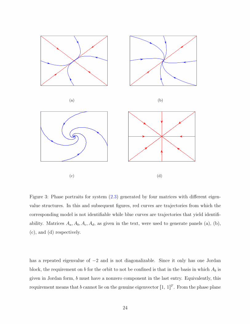
3 Phase portraits for system (2.3) generated by four matrices with different eigen-
value structures. In this and subsequent figures, red curves are trajectories
from which the corresponding model is not identifiable while blue curves are
trajectories that yield identifiability. Matrices Aa, Ab, Ac, Ad, as given in the
text, were used to generate panels (a), (b), (c), and (d) respectively. . . . . . 24
4 Phase space structures for matrix Ae. . . . . . . . . . . . . . . . . . . . . . . 25
5 Phase space structures for matrix Af . . . . . . . . . . . . . . . . . . . . . . . 26
6 Phase space structures for matrix Ag. . . . . . . . . . . . . . . . . . . . . . . 27
7 Confinement of φpA, bq in the flux space. . . . . . . . . . . . . . . . . . . . . . 33
8 paq Plot of the orbits for Ar with r “ 0, 1,´1, pbq Plot of the x component of
the trajectory. Each of the three distinct systems satisfy the data. . . . . . . 37
9 (a) Region R in y-space for which Φ P R2ˆ2 has two distinct positive eigenvalues
and hence Φ has a unique matrix logarithm, which solves the inverse problem.
(b)-(d) Regions in data space D for which Φ P R2ˆ2 has a unique matrix
logarithm, obtained as cross-sections of R formed by fixing two data points as
shown. For example, in pbq, x1, x2 are fixed and the shaded region indicates
where the coordinates of x0 can lie; note that pdq is strongly related to Figure
13. . . . . . . . . . . . . . . . . . . . . . . . . . . . . . . . . . . . . . . . . . 51
10 Region R in y-space for which Φ P R3ˆ3 has a unique matrix logarithm. . . . 52
ix

11 Trajectories of system (2.3) that share 5 data points in 5 dimensions need not
have the same dynamical behaviors. Each panel shows time courses of all 5
components of system (2.3) with n “ 5 for a particular choice of parameter
A. Within each panel, each color represents a different component of the
system, while the same components share the same color across panels. Five
points that are equally spaced in time, through which the trajectories pass in
all panels where trajectories exist, are marked with circles. The next equally
spaced point is labeled with a star; these points differ across panels and lead
to different properties of the inverse problem solution, including non-existence
of real parameter matrix for the data in the lower right panel. . . . . . . . . 53
12 Grid Mj surrounding a sample data point. . . . . . . . . . . . . . . . . . . . . 61
13 (a) Existence and uniqueness of matrix logarithm of Φ classified in terms of D
and T . (b) An example of how the existence and uniqueness of A depend on
the coordinates of x2, given fixed x0, x1. . . . . . . . . . . . . . . . . . . . . . 64
14 (a) Classification of the origin for (2.3) with A such that Φ “ eA, depicted in
terms of conditions on D “ det Φ and T “ tr Φ. Solid lines form boundaries
between regions; dashed lines do not. Note that the origin is a center for (2.3)
on the solid line separating stable and unstable spirals. (b) Conditions on the
position of x2 to give dynamical systems with specified equilibrium point types
when x0 and x1 are fixed. Solid lines form boundaries between regions; dashed
lines do not. . . . . . . . . . . . . . . . . . . . . . . . . . . . . . . . . . . . . 67
15 Numerical estimates of bounds ε associated with various inverse problem prop-
erties for data set in which x0 and x1 are fixed while x2 is varied. (a) Regions
where particular properties hold along with locations of x2 used in the esti-
mates. (b) Squares depict the numerically obtained bounds on the uncertainty
allowed to preserve stable node (red), stability (cyan), uniqueness (blue), and
nonexistence (green) properties. Coordinates of x2 and numerical values of the
bounds are listed in Table 1. . . . . . . . . . . . . . . . . . . . . . . . . . . . 69
x

16 (a) Numerical estimates, εU “ εSN (red), and εS (cyan) for data depicted. (b)
Stable node trajectory (red) that passes through the data d at equally spaced
time points and stable spiral trajectory (blue) through perturbed data d “
px0, x1, p3.1,´4.3qT q where d P Cpd, εSq but d R Cpd, εUq. . . . . . . . . . . . . 71
17 (a) Numerical estimates εS,“ εSN (red) and εU (blue) for the data depicted.
(b) Stable trajectory (red) through the data d and unstable trajectory (blue)
through perturbed data d P Cpd, εUq. . . . . . . . . . . . . . . . . . . . . . . . 72
18 The square regions surrounding the data point x2 represent numerical (red)
and analytical (green) . . . . . . . . . . . . . . . . . . . . . . . . . . . . . . . 73
19 Visual summary of the method used to compare the parameter density ρpaq
to the posteriors ρpa|ηq obtained using various priors πpaq in the Metropolis-
Hastings algorithm. . . . . . . . . . . . . . . . . . . . . . . . . . . . . . . . . 87
20 Visual summary of the method used to construct a sample of the parameter
density ρpaq to order to compare with posteriors ρpa|ηq obtained using various
priors πpaq in the Metropolis-Hastings algorithm. The red coloring indicates
the first density that is defined to begin the approach. . . . . . . . . . . . . 89
21 (a) In the phase plane, boundaries of the sets cpx1, εUq and cpx2, εUq are shown
in black, and the sample Y is depicted in green. (b) The marginalized density
function ηpyq is displayed black, and the blue histograms depict marginals of
the sample Y . . . . . . . . . . . . . . . . . . . . . . . . . . . . . . . . . . . . 92
22 Example 1: Curves representing marginalized histograms for A (red), MJeff
(blue), MUnif (black), and MJac (green). . . . . . . . . . . . . . . . . . . . . . 93
23 Example 2: Curves representing marginalized histograms for A (red), MUnif
(black), and MJac (green). . . . . . . . . . . . . . . . . . . . . . . . . . . . . . 94
24 Example 3: Curves representing marginalized histograms for A (red), MJeff
(blue), MUnif (black), and MJac (green). . . . . . . . . . . . . . . . . . . . . . 95
25 Visual summary of approach 2. The red coloring indicates the first density that
is defined to begin the approach. KDE refers to the kernel density estimation
of Y with a density ηpyq. . . . . . . . . . . . . . . . . . . . . . . . . . . . . . 97
xi

26 Example kernel density estimate for 4-dimensional data. Marginal histograms
of the data are shown in blue, marginals of the density estimate are given by
the red curves, and marginals of the kernels surrounding the data points are
given by the black curves. . . . . . . . . . . . . . . . . . . . . . . . . . . . . 99
27 Example kernel density estimate for 4-dimensional data. Two dimensional
projections of the discrete data set are pictured in (a) and projections of the
kernel density estimate are given in (b). . . . . . . . . . . . . . . . . . . . . . 99
28 Marginal histograms of Y are pictured, along with marginalizations of the
density ηpyq obtained from kernel density approximation, which are displayed
as red curves. The black curves represent the individual kernels which are
summed in the density estimation. In part (a) σ “ 0.15, (b) σ “ 0.2, and (c)
σ “ 0.25, all with the same mean parameter a “ p´1,´1.5,´1,´2q. . . . . . 101
29 Curves representing marginalized histograms for A (red), MUnif (black), and
MJac (green). In part (a) σ “ 0.15, (b) σ “ 0.2, and (c) σ “ 0.25, all with the
same mean parameter a “ p´1,´1.5,´1,´2q. . . . . . . . . . . . . . . . . . . 102
30 Marginalizations of the three different representations of the data are shown.
The point averaged representation is depicted by the green curve, the proba-
bility density function from the kernel density estimation is depicted by the
blue curve, and the histograms are shown in yellow . . . . . . . . . . . . . . . 105
31 Marginal histograms for A (red) and three estimates MJac obtained employing
kernel density estimation (blue), point averaged (green), and multidimensional
histogram (yellow). . . . . . . . . . . . . . . . . . . . . . . . . . . . . . . . . 105
32 Example 6: (a) Solutions curves from the mean parameter value and box plot
representations of Y . The box plots at t “ 1 for V and I are difficult to see
because they are tight relative to the figure scale. (b) marginal histograms
of Y and the kernel density estimate, (c) curves representing marginalized
histograms for A (red), MJeff (blue), MUnif (black), and MJac (green). . . . . 108
xii

33 Example 7: (a) Solutions curves from the mean parameter value and box plot
representations of Y . The box plots at t “ 1 for V and I are difficult to
see because they are tight relative to the figure scale. (b) curves representing
marginalized histograms for A (red), MJeff (blue), MUnif (black), and MJac
(green). . . . . . . . . . . . . . . . . . . . . . . . . . . . . . . . . . . . . . . . 109
34 Example 8: (a) Solutions curves from the mean parameter value and box plot
representations of Y . The box plot at t “ 3 for H is difficult to see because
it is tight relative to the figure scale. (b) curves representing marginalized
histograms for A (red), MJeff (blue), MUnif (black), and MJac (green). . . . . 110
35 Example 9: (a) Solutions curves from the mean parameter value and box plot
representations of Y . The box plot at t “ 2 for H is difficult to see because
it is tight relative to the figure scale. (b) curves representing marginalized
histograms for A (red), MJeff (blue), MUnif (black), and MJac (green). . . . . 111
36 Kernel density estimation in (a) one dimension, and (b), (c) two dimensions. 121
xiii

PREFACE
This work was supported in part by the National Science Foundation through grant EMSW21-
RTG 0739261.
There are several people I would like to thank for their support and dedication throughout
this long journey. I would first like to express my deepest gratitude to my joint research
advisors Dr. David Swigon and Dr. Jonathan Rubin, with whom I have had the pleasure of
working for more than five years. Throughout all of the ups and downs of graduate school, I
received encouragement and unwavering support from my advisors. I have always felt very
lucky to have two advisors because both of their intellectual and personal traits bring unique
contributions to our research team. I thank them for their patience in explaining concepts,
for their willingness to sit down with me to debug MATLAB code line by line, and for always
having an open door. Their guidance in our research investigations was invaluable and I have
grown immensely under their mentoring.
I would also like to thank my committee members, Dr. Catalin Trenchea and Dr. Gilles
Clermont. I appreciate their thoughtful questions and comments and their dedication, which
at times meant participating in a video conference while on vacation.
I would like to thank the Mathematical Biology group at the University of Pittsburgh and
the faculty, including my two advisors as well as Dr. Bard Ermentrout and Dr. Brent Doiron,
who organized the weekly seminars and research training group. My six year involvement in
the group was one of the most valuable experiences of my graduate career.
Thank you to my friend Jeremy Harris for in sharing the trials of graduate school and
for his help in studying for exams together.
My mother has been a pilar of support and a true friend, and I am eternally grateful for
her help.
xiv

I owe a great deal of gratitude to my husband, Chris, for encouraging me to pursue my
dreams. He has done a wonderful job caring for and raising our son while I was working. His
dedication made it possible for me to complete this work, and I couldn’t have accomplished
this without him. Thank you to my son, Isaac, for his abundant joy and positivity. There’s
nothing more inspiring in life.
I dedicate my dissertation in loving memory of my father Hurban Bolls. Thank you for
always telling me that you were proud of me.
xv
1.0 INTRODUCTION
The motivation for this investigation is rooted in the modeling of biological systems with
differential equations. In such an endeavor, one aims to model a physical phenomenon
to better understand it, explain it, reproduce it, and possibly to make predictions about
it. Insight can be gained through both quantitative and qualitative analysis of the model
equations. The advantages of employing differential equation models for biological systems
are discussed in [19]. In particular, the dynamics of how a system behaves over time, under
varying conditions can be captured using such a modeling approach.
Development of a model is a process consisting of several stages. First, the model struc-
ture for the system of interest is designed based on physical laws and a priori knowledge
of how certain components in the system interact. Model complexity is a fundamental is-
sue that must be confronted. The reductionist approach, in which small scale interactions
are studied, or the systemic approach, of representing higher levels of organization, may be
appropriate, depending on the modeling application [53, 60, 86]. Next, the identifiability
of model parameters is analyzed and the model is appropriately adjusted. Data about the
physical system is then collected using experimental studies, or already existing data is uti-
lized, and values of model parameters are estimated from the data. Further analysis of the
model is conducted and modifications to the model structure may be necessary. It is the
estimation of the parameters on which this work is focused.
Differential equation models of physical systems often involve parameters whose values
are not known and which may represent physical properties that cannot be directly measured.
Other model parameters might arise from approximations or model reductions and they may
have no direct biological interpretation [57]. Parameter estimation relies on the comparison
of experimental observations of the modeled system with corresponding model output to
1

obtain values for these parameters. Due to this, some assert that the usefulness of the model
is ultimately linked to the quality and abundance of the data [19]. Unfortunately, biologically
realistic models are likely to be parameter rich and data poor [7]. More recently, experimental
techniques such as microarray analysis, genome sequencing, high throughput flow cytometry
and ELISA biochemical assays, have made a wealth of biological data available for certain
applications [77].
Our particular interests stem from applications of mathematical modeling in medicine. In
this setting, experimental data often consists of time course measurements of test subjects
exposed to the same stimulus. In this work, we will refer to data collected from a single
subject at multiple points in time as single trajectory data. This data is often sparsely
available, for example, because an experiment is not repeatable due to the disease’s alteration
of the subject’s immune system [36, 62]. It is also common that not all model variables can
be measured. In this work, we will look at the problem of parameter estimation from single
trajectory data and collections of single trajectory data. We do not focus on a particular
application of mathematical modeling in biology, but instead try to address more broad
aspects of parameter estimation for dynamical systems.
Our investigation of parameter estimation from single trajectory data follows a natural
progression. We begin by examining an idealized setting with complete knowledge of an
entire trajectory of data which is free from error, and then we consider discrete points along
this trajectory. Next, we allow these discrete points to have uncertainty, and finally, we look
at the case of collections of discrete single trajectory data.
In the setting of error free data, we begin in Chapter 2, by addressing the question of
identifiability. A model is said to be identifiable if the parameter estimation problem has a
unique solution given some amount of error free data. Identifiability analysis is an a priori
study that should be conducted once a model structure has been fixed. It is important
to establish identifiability prior to implementing computational techniques for parameter
estimation to avoid misinterpretation of the numerical results.
There is a rich body of literature addressing identifiability for both linear and nonlinear
systems of differential equations, [8, 9, 44, 58, 63, 89]. For linear systems of differential
equations, the transfer function method utilizes Laplace transforms of the model equations
2

to derive a response function whose coefficients determine identifiability [8]. This method ul-
timately relies on the ability to solve simultaneous nonlinear equations. In another approach
for linear systems, power series expansions of the trajectory as a function of the unknown
parameters are analyzed to determine identifiability [89]. Alternatively, instead of trying
to identify the parameter matrix of the linear system directly, the modal matrix approach
aims to identify the eigenvalues and eigenvectors of the matrix [44]. These methods are
only feasible for low dimensional systems as the analysis becomes difficult or impossible as
dimensions increase. For nonlinear systems of differential equations, a differential algebra
approach employs differential polynomials to define an input-output relation with rational
coefficients which depend on the model parameters. These coefficients are used to define a
map whose injectivity determines the identifiability. Computer algorithms have been intro-
duced to perform the symbolic computations required for the differential algebra approach
[9]. Another approach for nonlinear systems is the implicit function method. Here, deriva-
tives of the system outputs with respect to time are taken and any unobservable system states
are eliminated. Then the rank of a matrix whose entries consist of partial derivatives with
respect to the parameters determines the identifiability of the system [90]. In this approach,
higher order derivatives can become complicated and the singularity of the matrix can be
difficult to determine [63]. Each of these treatments are highly reliant on computations that
are only feasible in low dimensions or with the help of computer programs. Also, in the
methods discussed above, the models typically include an input which serves as a control
for the system. Identifiability is then addressed with full access to the set of all admissible
controls. Our treatment is instead geared toward the case of single trajectory data. Without
access to a set of controls, resulting in a variety of observations for the system, we have only
a single initial condition, and thus one trajectory, from which to determine the parameters.
This work complements this existing literature and approaches the identifiability problem in
a uniquely different way, see Figure 1.
In Chapter 2, we investigate identifiability by asking whether the parameters of linear and
linear-in-parameters dynamical systems can be uniquely determined from a single trajectory.
We provide precise definitions of several forms of identifiability, and derive some novel,
interrelated conditions that are necessary and sufficient for these forms of identifiability to
3

Figure 1: Features of our investigations of identifiability compared to those of existing meth-
ods.
arise. We also show that the results have a direct extension to a class of nonlinear systems
that are linear in parameters. One of our results provides information about identifiability
based solely on the geometric structure of an observed trajectory, while other results relate
to whether or not there exists an initial condition that yields identifiability of a fixed but
unknown coefficient matrix and depend on its Jordan structure or other properties. Several
examples are presented to illustrate identifiability for various systems and trajectories. In the
later part of the chapter, we transition to looking at identifiability from a discrete collection
of data points along a trajectory. By considering data that are observed at equally spaced
time intervals, we form a special matrix whose Jordan structure determines the identifiability.
Lastly, we show that the sensitivity of parameter estimation with discrete data depends on
a condition number related to the data’s spatial confinement. The content of this chapter
appeared as a publication in [76].
In Chapter 3, we continue our study of parameter estimation with discrete data from
a single trajectory and extend the investigation to consider the case of uncertainty in the
data. The problem of estimation of parameters of a dynamical system from discrete data
can be formulated as the problem of inverting the map from the parameters of the system
to points along a corresponding trajectory. Solving the inverse problem becomes even more
4

challenging in the presence of uncertainty in experimental measurements, as may arise due
to measurement errors and fluctuations in system components. In Chapter 3, we focus on
linear systems of differential equations and derive necessary and sufficient conditions for
single trajectory data to yield a matrix of parameters with specific dynamical properties.
To address the key issue of robustness, we go on to establish conditions that ensure that
the desired properties of the solution to the inverse problem are maintained on an open
neighborhood of the given data. We then build from these results to find bounds on the
maximal uncertainty in the data that can be tolerated without a change in the nature of
the inverse problem. In particular, both analytical and numerical estimates are derived for
the largest allowable uncertainty in the data for which the qualitative features of the inverse
problem solution, such as uniqueness or attractor properties, persist. We also derive the
conditions and bounds for the non-existence of a real parameter matrix corresponding to
the given data, which can be utilized in modeling practice to prescribe a level of uncertainty
under which the linear model can be rejected as a representation of the data. One result
establishes regions in data space on which uniqueness of the inverse problem solution is
guaranteed. The invertibility of the solution map on these sets will play a vital role in the
analysis of Chapter 4. Regions in data space on which the inverse problem maintains a
unique solution can also be mapped back to define regions in parameter space on which the
model is identifiable. The contents of this chapter have been submitted for publication and
are currently undergoing review.
Our final study relates to the practical problem of parameter estimation given a collection
of discrete single trajectory data. As we have seen, such a collection of data may arise from
time series data which was measured experimentally from several individuals in a population.
This situation provides the motivation for our study and presents several challenges in the
parameter estimation problem. If the parameters of the model have biological significance, for
example virus clearance rate or initial concentration of virus particles, it is natural for their
values to vary from individual to individual within a population. With this perspective, the
solution to the inverse problem is not a single parameter value, but instead, is a distribution
of parameters representing variability over a population [77]. The objective is then to find
the best approximation to the parameter density that describes this distribution. In a
5
Bayesian inference approach to parameter estimation, the parameter density is approximated
by a posterior density, which makes use of the data that is available for the system. An
introduction to Bayesian inference for parameter estimation can be found in [33, 74]. The
posterior density is formed using a likelihood function, which quantifies the deviation of the
model from the available data, and a prior density which incorporates any previous knowledge
about the parameters. A sample of the posterior can be constructed using Markov chain
Monte Carlo techniques, and in particular the Metropolis-Hastings algorithm. Several recent
papers have used the Metropolis-Hastings algorithm for Bayesian parameter estimation in
models of infectious disease and intrahost response to bacterial and viral infections, [59, 64,
65, 69].
Prescription of a likelihood function and prior density are necessary to implement Bayesian
parameter estimation. The prior density reflects any information that is known about the
parameters before data is considered, which may include bounds on the values of the pa-
rameters which are obtained from literature (e.g. biological experiments) or from qualitative
analysis of the system (e.g. analysis of existence and stability of equilibria). A nonin-
formative prior (also commonly referred to as an objective or flat prior) is used when no
information about the parameter values is known. Alternatively, an informative prior can
be used when characteristics of the parameters are known a priori. Unlike noninformative
priors, informative prior is not dominated by the likelihood. The choice of a prior is a topic
of intense debate among practitioners of Bayesian inference [10, 32, 68, 74]. In Chapter 4, we
contribute to the conversation on prior density selection by introducing a new informative
prior density called the Jacobian prior, which exploits knowledge of the fixed model structure,
Figure 2. After presenting a theoretical derivation of the prior, we develop two approaches
to systematically analyze the accuracy of the posterior density obtained by implementing
the Metropolis-Hastings algorithm with the Jacobian prior. In first approach, we employ
a linear system of differential equations and use key results of Chapter 3 to define the pa-
rameter density solution to the inverse problem as means for comparison with the posteriors
obtained from the Metropolis-Hastings algorithm. The posterior obtained with the Jacobian
prior is compared to the parameter density and to other posteriors that are computed using
two other commonly employed priors. The second approach can be used with any system
6

Figure 2: Our contribution to the problem of prior density selection.
of differential equations; we apply it again with the linear system and then with a nonlinear
model. For the linear system of differential equations, there is a clear evidence that the
Jacobian prior makes the posterior a better approximation of the parameter density. In the
nonlinear case, the posterior is approximated more accurately with the Jacobian prior in
some cases and equally well using all three of the priors in other cases.
7

2.0 IDENTIFIABILITY OF LINEAR AND LINEAR-IN-PARAMETERS
DYNAMICAL SYSTEMS FROM A SINGLE TRAJECTORY
2.1 INTRODUCTION
Mathematical models of physical systems often include parameters for which numerical values
are not known a priori and cannot be directly measured. Parameter estimation relies on the
comparison of experimental observations of the modeled system with corresponding model
output to obtain values for these parameters. There are many computational techniques
for parameter estimation that can be employed, most of which rely on minimization of the
difference between model output and observed data. However, before numerical estimates
of parameter values are pursued, it is important to address the question of whether the
parameters of the model are identifiable; that is, does the parameter estimation problem have
a unique solution, given access to some amount of error free data? If the model’s parameters
are not identifiable from such idealized data, then numerical estimates of parameters from
data may be misleading. Clearly, the answer to this question depends on the structure of
the underlying model, the amount and type of the data given, and the precise definition of
uniqueness.
Identifiability analysis of dynamical systems has been an area of intense study [8, 15, 18,
63, 67, 89] and it is usually employed to aid model development, which ideally proceeds in the
following order: first a model of a system of interest is designed; second, the identifiability
of model parameters is analyzed and the model is appropriately adjusted; third, sufficient
amount of data about the physical system is collected using experimental studies; and finally,
values of model parameters are estimated from the data. In many biological studies, however,
the order is often reversed, and modelers use data that were collected before any thought was
8

given to modeling of the system. The modeler then faces the challenging task of designing a
model that represents and explains the existing data for a system that is no longer available
or for which measurements cannot be repeated under the original conditions. In some cases,
repeated collection of data from a single subject is impossible because it has been destroyed
during the process of data collection. This happens frequently in studies of disease models
in clinical settings, in which either the disease itself or the manipulations performed to assay
the subject’s state may be fatal to the subject (laboratory animal). In immunological studies
on mice, for example, each data point is an aggregate of data obtained from several different
animals which are sacrificed during the process [82, 46]. In disease studies on larger mammals
or humans, longitudinal data may be obtained for a single subject, but the experiment is not
reproducible because the subject’s immune system has been altered by the disease [36, 62].
In this chapter we take this problem to the extreme and address the question of identifiability
of parameters of dynamical systems from a single observed trajectory.
Linear models are a natural starting point for our study because they have a simple
structure, but the identifiability question in this setting is nonetheless nontrivial because
the solution to such a system depends nonlinearly on its parameters. This setting is also
convenient because there is existing theory to build on and one can exploit invertible op-
erators for numerical techniques for handling linear systems. Parameter identifiability for
linear dynamical systems has been studied extensively in control theory and related areas
[8, 30, 34, 48, 67, 70, 88, 89]. A time-invariant linear control model typically has the form
9xptq “ Axptq `Buptq
yptq “ Cxptq(2.1)
where A,B,C are parameter matrices, xptq is a vector function that defines the state of the
system at time t, uptq is the vector of input (control), and yptq is the vector output. Zero
initial conditions are typically chosen, but delta-function controls can be used to represent
any desired initial condition. The impulse response function Y psq “ CpsI ´ Aq´1B fully
describes the (Laplace transformed) solutions of the system. In this context the matrix pa-
rameters A,B,C are said to be identifiable if they can be determined from the set of output
9

observations y obtained by varying the control u. It is known that even with all control func-
tions available, the matrices A,B,C are not all simultaneously identifiable, since the impulse
response function is invariant under the transformation pA,B,Cq Ñ pT´1AT, T´1B,CT q,
where T is an invertible matrix [8]. Kalman [48] devised a nomenclature in which the system
(2.1) is transformed into a new set of variables that can be divided into four classes: (a) con-
trollable but unobservable, (b) controllable and observable, (c) uncontrollable and unobserv-
able, and (d) uncontrollable but observable. Bellman and Astrom showed that if C is square
and has full rank (i.e., all states x are observable) and the matrix rB |AB | ¨ ¨ ¨ |An´1Bs has
full rank (i.e., the system is controllable), then both A and B are identifiable from the im-
pulse response of the system when a full set of controls is available [8]. In special situations
in which the matrices A,B,C depend on a parameter, that parameter may be identifiable
even when C does not have full rank. It is not clear whether enough information can be
obtained to identify the parameters from a smaller set of controls, perhaps even a single
trajectory (i.e., single control), however, which is all that may be available in our motivating
applications. Sontag has shown that when the model is identifiable, the parameters can be
estimated even from information about a single variable extracted from a single trajectory,
provided that enough data points have been measured: no more than 2r` 1 data points are
required to identify r parameters in the case in which the dynamical system is real analytic
[75]. Since the classical results discussed above imply that C must be full rank for identi-
fiability to be possible, we predominantly focus here on the case in which C is full rank in
(2.1), in which case, without loss of generality, we can in fact assume that C “ I. However,
we also briefly consider the issue of partial identifiability when C is of lower rank.
As the next step, we examine nonlinear dynamical systems that depend linearly on
parameters. Such systems can be written in the form
9xptq “ Afpxptqq ` uptq ´ µptqxptq (2.2)
where A is a parameter matrix, f is a known, locally Lipschitz continuous map (to insure
existence and uniqueness of solutions), uptq is a time-dependent input and µptq is a decay
control. Such systems commonly arise in differential equation models of chemical reaction
networks that are derived from mass-action kinetics; in those cases, A is the stoichiometric
10

matrix, f is the vector of reaction rate functions (each of which is a product of a reaction
rate constant and a monomial in the components of x), u is the inflow into the reaction
chamber, and µ is the outflow [41, 24, 25]. Among models of type (2.2) one can also include
the generalized Lotka-Volterra models that are commonly used in ecology or population
dynamics [21, 66, 43], in which cases A is usually a sparse matrix. The problem of identifying
the model (2.2) consists of two separate tasks: (i) identification of the parameter matrix A
and (ii) identification of the reaction rate functions fpxq. Each of these problems has been
studied extensively [38, 84, 50]. Several conditions for identifiability have also been derived.
For example, Chen and Bastin [13] found necessary and sufficient conditions for identifiability
of A in the case when full response of the system to the controls u and µ is available. Farina et
al. [23] addressed the problem of identifying the reaction rate constants in fpxq by expanding
the system and linearizing about an equilibrium state and found that the Jacobian must be
full rank and that knowledge of dynamical data for any time-dependent input to the system
is essential. Craciun and Pantaea [16] related the identifiability of chemical reaction network
systems to the topology of the reaction network. Here we assume that the functions fpxq
are known and focus on task (i).
We begin in Section 2.2 by presenting several definitions of identifiability and review-
ing established theorems on identifiability for linear dynamical systems. In Section 2.3, we
expand on these results to provide a complete rigorous characterization of identifiability
from a single trajectory for linear dynamical systems. More specifically, we discuss several
equivalent characterizations of the identifiability criterion, which ultimately yield an iden-
tifiability condition solely based on geometric properties of the known trajectory, namely
whether or not the trajectory is confined to a proper subspace of the relevant phase space.
This criterion provides practical utility, since it can be applied using what is known about
the trajectory, without knowledge of the structure of the parameter matrix. Subsequently,
we investigate the existence of a trajectory for which the parameter matrix is identifiable,
obtaining a necessary and sufficient requirement for existence based on the properties of the
coefficient matrix associated with the model. Several examples illustrate identifiability for
various systems and initial conditions. In Section 2.4, we briefly discuss some implications
of our confinement result for partial identifiability and for identifiability when not all model
11

variables are observable. In Section 2.5, we extend our results to a broader class of dynamics
by deriving necessary and sufficient conditions for identifiability of a nonlinear system that is
linear in parameters. The sufficient condition again has geometrical character and refers to
the confinement of an image of the trajectory in the space of reaction rates. In Section 2.6,
we discuss the problem of finding parameter values explicitly using discrete data and show
that some linear models are identifiable from a complete trajectory but not from a finite set
of data, and that the accuracy of parameter estimation is related to how significantly the
available data deviates from confinement. The chapter concludes with a brief summary of
results and possible future directions in Section 2.7.
2.2 DEFINITIONS AND PRELIMINARIES
We consider a model defined as a linear dynamical system in which data for all of the state
variables is available (i.e. C “ I) and the set of inputs (controls) consists of the set of initial
conditions:
9xptq “ Axptq
xp0q “ b.(2.3)
In equation (2.3), xptq P Rn is the state of the system at time t, the system parameters are
the entries of the coefficient matrix A P Rnˆn, and b P Rn is the initial condition. For clarity
of exposition we will refer to the entire matrix A as the (matrix) parameter A. Analysis of
linear systems of the form (2.3) is greatly simplified since we have an explicit formula for
their solutions, which we generally refer to as trajectories:
xpt;A, bq “ eAtb “8ÿ
j“0
Ajtj
j!b. (2.4)
In the context of this work the term model identifiability is meant to represent the
identifiability of the parameters of the model. In other words, we fix the model structure
and ask whether the matrix parameter A can be uniquely determined from error-free data
consisting of a trajectory or some subset thereof. This question is strongly related to whether,
independent of the data, two distinct parameters can lead to identical solutions. A term
12
parameter distinguishability has been used in this context in the literature [15, 34]. It is
clear that these characteristics depend not only on the properties of the system, but also on
the set of possible parameters being considered for comparison. The identifiability problem
should therefore be reformulated as determining whether, on a particular subset of Rnˆn,
the map from parameter space to solution space is injective. The extreme cases are to
allow parameters from the full parameter space Rnˆn or to restrict to a single point in the
parameter space. In the latter case, identifiability is trivial since there are no other competing
parameters to consider.
The initial condition b determines the trajectory (2.4) of the system (2.3) uniquely for any
given A. It needs to be taken into consideration, since we may or may not know or be able
to select the initial values of the states represented in a model before running an experiment,
and hence we may wish to consider identifiability from a given initial condition or from a
larger set of initial conditions. We shall discuss here three progressively more constrained
definitions of identifiability. In the first definition, we allow for an initial condition to be
chosen to aid identifiability:1
Definition 1. Model (2.3) is identifiable in Ω Ď Rnˆn if and only if for all A,B P Ω, A ‰ B,
there exists b P Rn such that xp¨;A, bq ‰ xp¨;B, bq.2
For identifiability in the sense of Definition 1, we immediately have the following result:
Theorem 2. Model (2.3) is identifiable in Rnˆn.
Proof. Consider the negation of the statement: model (2.3) is not identifiable in Ω if there
exist A,B P Ω, A ‰ B, such that for all b P Rn, for all t P R, xpt;A, bq “ xpt;B, bq. This
negation cannot hold on a set Ω containing distinct elements A and B, since if xpt;A, bq “
xpt;B, bq for all b P Rn, for all t P R, then differentiation of equation (2.4) and evaluation
at t “ 0 gives Ab “ Bb for all b. Applying this result to n linearly independent choices of
b gives AW “ BW for the invertible matrix W with the selected b vectors as its columns,
1The definitions above employ the term identifiability in the same sense in which global identifiability hasbeen used in some literature (e.g., [80]) to distinguish this concept from that of local identifiability, whichfocuses on a small neighborhood of a given parameter. However, since Ω may be just a proper subset of thefull parameter space, the use of the word global in this context could be misleading and thus we omit it.
2The notation xp¨;A, bq ‰ xp¨;B, bq indicates that there exists at least one t ą 0 such that xpt;A, bq ‰xpt;B, bq. Analogously, xp¨;A, bq “ xp¨;B, bq indicates that xpt;A, bq “ xpt;B, bq are identical for all t.
13

hence A “ B. As a consequence, we see that for any two distinct linear systems (2.3), there
is an initial condition b P Rn that will distinguish the solutions.
Theorem 2 implies that if we are free to choose the initial condition, then any two linear
models with distinct parameter matrices in Rnˆn can be distinguished, because we can
choose the initial condition b such that the corresponding trajectories will be distinct. In
practice, however, control over the initial condition may not be available, and more restrictive
definitions of identifiability are needed. Nonetheless, Definition 1 is important in a setting
in which the matrix A itself is parametrized by an auxiliary parameter. For example, for
9x “ pp1 ` p2qx, the parameter sets pp1, p2q “ pc1, c2q and pp1, p2q “ pc2, c1q will result in the
same trajectory, with no initial condition b that will distinguish them.
Identifiability from a single trajectory is addressed by the following definition:
Definition 3. Model (2.3) is identifiable in Ω from b P Rn if and only if for all A,B P Ω
with A ‰ B, it holds that xp¨;A, bq ‰ xp¨;B, bq.
Since in most practical applications with biological data, the initial condition is fixed
and cannot be chosen at will, most of our results in Section 2.3 relate to identifiability in the
sense of Definition 3. It is also of interest, however, to consider the problem of identifiability
from any initial condition:
Definition 4. Model (2.3) is unconditionally identifiable in Ω if and only if for all A,B P
Ω, A ‰ B implies that for each nonzero b P Rn, xp¨;A, bq ‰ xp¨;B, bq.
Sufficient conditions for unconditional identifiability will be revealed in the end of Section
2.3.
We will now show that necessary and sufficient conditions for identifiability of model
(2.3) in the sense of Definition 3 follow from published results of Thowsen [80] and Bellman
and Astrom [8]. First, suppose that Ω is an open set, in which case we have:
Theorem 5. For Ω Ă Rnˆn open and a fixed b P Rn, model (2.3) is identifiable in Ω from b
if and only if tb, Ab, ..., An´1bu are linearly independent for all A P Ω.
Remark. An alternative but equivalent formulation would replace the condition of linear
independence with the condition that the matrix rb|Ab|...|An´1bs has full rank, which would
14

bring the wording closer to that of Bellman and Astrom.
We will obtain Theorem 5 from the following theorem, presented by Thowsen [80] (and
simplified later by Gargash [28]), which we state without proof:
Theorem 6. Let Ω Ă Rnˆn be a set of matrices such that Ω “ třpj“1Ajαj|α P Θu, where
Aj P Rnˆn for all j and Θ is an open subset of Rp. Fix b P Rn and let
GpAq “
»
—
—
—
—
—
—
—
–
A1b . . . Apb
A1Ab . . . ApAb...
. . ....
A1An´1b . . . ApA
n´1b
fi
ffi
ffi
ffi
ffi
ffi
ffi
ffi
fl
n2ˆp
Model (2.3) is identifiable in Ω from b if and only if rankGpAq “ p for all A P Ω.
Proof. (of Theorem 5) Consider the decomposition of A into elementary matrices, A “
řni,j“1Eijaij where tEiju is the standard basis for nˆ n matrices, and the set Θ is equal to
Rn2. Under this decomposition, the matrix GpAq in Theorem 6 takes the special form GpAq “
»
—
—
—
—
—
—
—
—
—
—
—
—
—
–
E11b E12b . . . Ennb
´´´ ´´´ ´´´ ´´´
E11Ab E12Ab . . . EnnAb
´´´ ´´´ ´´´ ´´´...
.... . .
...
´´´ ´´´ ´´´ ´´´
E11An´1b E12A
n´1b . . . EnnAn´1b
fi
ffi
ffi
ffi
ffi
ffi
ffi
ffi
ffi
ffi
ffi
ffi
ffi
ffi
fl
“
»
—
—
—
—
—
—
—
—
—
—
—
—
—
—
—
—
—
—
—
—
—
—
—
—
—
—
—
—
—
—
—
—
—
—
–
bT 0 . . . 0
0 bT . . . 0...
... . . ....
0 0 . . . bT
´´´ ´´´ ´´´ ´´´
pAbqT 0 . . . 0
0 pAbqT . . . 0...
... . . ....
0 0 . . . pAbqT
´´´ ´´´ ´´´ ´´´...... . . .
...´´´ ´´´ ´´´ ´´´
pAn´1bqT 0 . . . 0
0 pAn´1bqT . . . 0...
... . . ....
0 0 . . . pAn´1bqT
fi
ffi
ffi
ffi
ffi
ffi
ffi
ffi
ffi
ffi
ffi
ffi
ffi
ffi
ffi
ffi
ffi
ffi
ffi
ffi
ffi
ffi
ffi
ffi
ffi
ffi
ffi
ffi
ffi
ffi
ffi
ffi
ffi
ffi
ffi
fl
15

Let
GpAq “
»
—
—
—
—
—
—
–
bT
pAbqT
...
pAn´1bqT
fi
ffi
ffi
ffi
ffi
ffi
ffi
fl
nˆn
.
With this definition, rankGpAq “ n ¨ rank GpAq. Hence, rankGpAq “ n2 if and only if
rank GpAq “ n, which holds if and only if tb, Ab, ..., An´1bu are linearly independent.
Next, we note that the sufficiency of the condition of linear independence of tb, Ab, ..., An´1bu
is not tied to the requirement that Ω is an open set. This observation becomes obvious from
a reformulation of a result of Bellman and Astrom obtained for the control system (2.1) [8]:
Theorem 7. For Ω Ă Rnˆn and a fixed b P Rn, if tb, Ab, ..., An´1bu are linearly independent
for all A P Ω, then model (2.3) is identifiable in Ω from b.
Let us define, for a fixed b P Rn, the set Ωb “ tA P Rnˆn : tb, Ab, ..., An´1bu are linearly
independentu. This set has a special significance for the identifiability of the model from b
in view of the following corollary of Theorem 5:
Corollary 8. Let b P Rn be fixed. The set Ωb is the largest open set in which model (2.3) is
identifiable from b.
Proof. Clearly, by Theorem 5, any open set Ω Ď Rnˆn in which the model (2.3) is identifiable
from b satisfies Ω Ď Ωb. That Ωb is an open set follows from Corollary 18, which is stated at
the end of the next Section.
In view of Theorem 5, the sets Ωb can be employed to characterize sets Ω in which the
model (2.3) is unconditionally identifiable:
Corollary 9. Let Ω P Rnˆn be open. Model (2.3) is unconditionally identifiable in Ω if and
only if Ω ĎŞ
bPRnzt0u Ωb.
Although the conditions stated in Theorems 5, 7, and Corollary 9 reveal the properties
of sets in which the model is identifiable, their practical applicability is limited, because we
cannot test whether the system obeys the condition A P Ωb unless we know the matrix pa-
rameter A. In the next section, we derive a more practical condition based on the properties
16

of a model trajectory. That is, let γpA, bq “ txpt;A, bq : t P Ru Ă Rn denote the orbit of
the model (2.3) corresponding to the trajectory with initial condition b. The condition that
we obtain specifies, for any given trajectory, whether or not we can identify the model from
that trajectory. Specifically, we show that the model (2.3) is identifiable from a trajectory if
and only if the orbit corresponding to that trajectory is not confined to a proper subspace
of Rn.
2.3 IDENTIFIABILITY CONDITIONS BASED ON TRAJECTORY
BEHAVIOR OR COEFFICIENT MATRIX PROPERTIES
2.3.1 Analysis
Now that we have established that the identifiability of the model from a fixed initial con-
dition b is characterized by the linear independence of the set tb, Ab, ..., An´1bu, we will
discuss certain equivalent characterizations of that property that reveal its implications for
the geometrical behavior of the corresponding orbit.
We will denote the space formed by linear combinations of the vectors tb, Ab, ..., An´1bu
as KnpA, bq “spantb, Ab, ..., An´1bu. This space is the Krylov subspace generated by A and
b [92] which is also called the A-cyclic subspace generated by b [40] and is the range of the
controllability matrix rb |Ab | ¨ ¨ ¨ |An´1bs.
Lemma 10. tb, Ab, ..., An´1bu are linearly dependent, or equivalently dimpKnpA, bqq ă n, if
and only if b is contained in an A-invariant proper subspace of Rn.
Proof. Recall that a space V is called A-invariant if for all v P V,Av P V . For the forward
direction, assume that dimpKnq ă n. Certainly, b P Kn. The result thus follows from
showing that Kn is invariant under A. To establish this invariance, let x P Kn. Then,
x “ c0b ` c1Ab ` ... ` cn´1An´1b and Ax “ c0Ab ` c1A
2b ` ... ` cn´1Anb. By the Cayley-
Hamilton Theorem, An can be written as a linear combination of I, A,A2, ..., An´1. Hence,
Ax “ d0b` d1Ab` ...` dn´1An´1b P Kn, as desired.
17

The reverse direction follows immediately, as b P V for an A-invariant set V with
dimpV q ă n implies that, since Kn Ď V , dimpKnq ď dimpV q ă n as well.
Lemma 11. Orbit γpA, bq is confined to a proper subspace of Rn if and only if b is contained
in an A-invariant proper subspace of Rn.
Proof. For the backward direction, let V Ă Rn be an A-invariant proper subspace of Rn. If
b P V , then Ajb P V for all j “ 0, 1, .... Hence, xpt;A, bq “ eAtb “8ÿ
j“1
tjAjb
j!P V for all
t P R. So, γpA, bq Ď V .
For the forward direction, assume that γpA, bq is confined to a proper subspace of Rn.
Then there exists v ‰ 0 P Rn such that vTxpt;A, bq “ 0 for all t P R. Since xpt;A, bq “ eAtb,
we have vT eAtb “ 0 for all t P R as well. Furthermore, differentiation gives vTAeAtb “
0, . . . , vTAjeAtb “ 0 for all t P R, for j “ 0, 1, ..., n´ 1. In particular, for t “ 0, vTAjb “ 0
for j “ 0, 1, ..., n ´ 1. Hence, vT rb Ab...An´1bs “ 0. Since v ‰ 0, rb Ab...An´1bs cannot have
full rank, and thus Lemma 10 gives the desired result.
In light of Theorem 5, Lemmas 10 and 11 yield the following corollary:
Corollary 12. For Ω Ă Rnˆn open, model (2.3) is identifiable in Ω from b if and only if for
all A P Ω, γpA, bq is not confined to a proper subspace of Rn.
Combining the above results we obtain one of the main results of this chapter, a concise
relation between the uniqueness of the parameters of the model (2.3) and the geometric
structure of its orbits:
Theorem 13. For the model (2.3) there exists no B P Rnˆn with A ‰ B such that xp¨;A, bq “
xp¨;B, bq if and only if the orbit γpA, bq is not confined to a proper subspace of Rn.
Proof. Suppose that the orbit γpA, bq of model (2.3) is not confined to a proper subspace
of Rn, i.e., the parameter matrix A that supplied the orbit obeys A P Ωb. If B P Ωb
with A ‰ B, then the trajectories xpt;A, bq and xpt;B, bq are distinct as a result of the
identifiability of the model (2.3) in Ωb from b. If, on the other hand, B R Ωb, then the set
of vectors tb, Bb, ..., Bn´1bu is linearly dependent and hence Lemmas 10 and 11 imply that
18

the orbit γpB, bq is confined to a proper subspace of Rn. Therefore xpt;B, bq is not equal to
xpt;A, bq.
Theorem 13 implies that the parameter matrix of model (2.3) is uniquely defined by
any trajectory that has an orbit that is not confined to a proper subspace. It is a practical
result that provides immediate information about the possibility of model identification
from a single trajectory while relying solely on the geometrical description of the trajectory.
Note that the full trajectory is needed to identify the matrix A since the orbit provides no
information about the transit time.
With this relation of identifiability to trajectory behavior, we can also observe that
identifiability is invariant under similarity transformation.
Corollary 14. Model (2.3) is identifiable in Ω P Rnˆn from b P Rn if and only if model (2.3)
is identifiable in ΩS “ tC “ SAS´1 : A P Ωu from Sb, for all S P Rnˆn invertible.
Proof. For the forward direction, assume that model (2.3) is identifiable in Ω from b and let
A P Ω. Let S be an invertible nˆ n matrix and define C “ SAS´1. Assume C and D yield
the same trajectory for the initial condition Sb. Since C and D yield the same trajectory,
eCtSb “ eDtSb and hence eS´1CStb “ eS
´1DStb and eAtb “ eS´1DStb, for all t P R. Since A
is identifiable from b, A “ S´1DS. So, SAS´1 “ D, which yields C “ D. Hence, model
(2.3) is identifiable in Ω from Sb, for all S P Rnˆn invertible. The reverse direction follows
similarly.
Having related identifiability on Ω to the linear independence of tb, Ab, ..., An´1bu for
A P Ω, it is natural to ask whether for every parameter matrix A the set Ωb is non-empty,
i.e., whether for every A there is an initial condition b such that such that tb, Ab, ..., An´1bu
are linearly independent. We will now show that such a b need not necessarily exist and
hence there are models (2.3) that cannot be identified from any single trajectory.
The following result determines under what conditions on the structure of A the set Ωb
is non-empty.
Theorem 15. There exists b such that tb, Ab, ..., An´1bu are linearly independent if and only
if A has only one Jordan block for each of its eigenvalues.
19

Proof. The result follows from Cyclic Decomposition Theorem for square matrices. In par-
ticular, a vector b such that tb, Ab, ..., An´1bu are linearly independent is called a cyclic vector
for A. A corollary of the Cyclic Decomposition Theorem ([40] p. 237) states that A has a
cyclic vector if and only if the characteristic and minimal polynomials for A are identical,
which holds if and only if the matrix A has only one Jordan block for each of its eigenvalues.
This condition results from the fact that a nilpotent matrix pJ´λIq, where J is an kˆk
elementary Jordan matrix with eigenvalue λ, has minimal polynomial of the form xk, and
furthermore the minimal polynomial of A is of order m “řsi“0 ki where ki is the size of the
largest Jordan block corresponding to the eigenvalue λi of A, with the sum being taken over
all distinct eigenvalues of A. Now, the property that A has only one Jordan block for each of
its eigenvalues holds if and only if m “řsi“0 ki “ n, which is equivalent to the characteristic
and minimal polynomials for A being identical.
An additional Proposition elucidates a certain structure for b that is useful for attaining
identifiability.
Proposition 16. For a k ˆ k elementary Jordan matrix J with eigenvalue λ and vector
b P Rk with bk ‰ 0, pJ ´ λIqmb “ 0 if and only if m ě k.
Proof. The backward direction is immediate since for m ě k, pJ ´ λIqm “ 0. The forward
direction follows because for p ă k, pJ ´ λIqpb “ rbp`1, . . . , bk, 0, . . . , 0sT ‰ 0 whenever
bk ‰ 0.
Theorem 15 establishes the existence of b from which model (2.3) is identifiable under
the linear independence condition and Proposition 16 specifies a structure for such b. In
particular, for such b, the component corresponding to each ki ˆ ki Jordan block Ji of A
must not be annihilated by pJi ´ λiIqki´1. For diagonalizable A, this result reduces to the
requirement that such b has a nonzero component in each eigenspace of A (see Lee [56]).
This property, sometimes referred to as persistent excitability for systems in control theory,
has been discussed by [5, 58]. A result closely related to Theorem 15 can be found in [52].
More interesting examples arise for matrices that do not have distinct real eigenvalues and
are discussed in examples below.
20

Another helpful characterization of the linear independence of tb, Ab, ..., An´1bu can be
stated in terms of left eigenvectors of A, using the well known PBH controllability test for
linear systems [47]:
Theorem 17. The vectors tb, Ab, ..., An´1bu are linearly independent if and only if there is
no left eigenvector of A orthogonal to b.
In our case we employ this theorem for the following result:
Corollary 18. For Ω Ă Rnˆn open, model (2.3) is identifiable in Ω from b if and only if
there is no left eigenvector of A orthogonal to b for any A P Ω.
The Corollary 18 provides a new criterion for identifiability of the model (2.3) and can
be used to characterize the set Ωb from Section 2: Ωb “ tA P Rnˆn : wTA “ λw ñ wT b ‰ 0u
defines the largest open set in which the model is identifiable from b. Likewise,
č
bPRnzt0u
Ωb “ tA P Rnˆn : wTA “ λw ñ wT b ‰ 0 for all b P Rnzt0uu
defines the largest set Ω in which the model is unconditionally identifiable.
For matrices of even dimensions we can use this representation to define sets Ω in which
model (2.3) is unconditionally identifiable. For example, let Ωc “ tA P R2ˆ2 : A has a
complex pair of eigenvaluesu. Any left eigenvector w of a matrix A in this set has nonzero
imaginary part and hence w is not orthogonal to any vector b P R2. By Corollary 18, tb, Abu
are linearly independent (over R), hence the model is unconditionally identifiable in Ωc by
Corollary 9.
Interestingly, matrices with odd dimensions always have a real-valued left eigenvector
w and our results imply that there is no set Ω Ď Rp2n`1qˆp2n`1q in which model (2.3) is
unconditionally identifiable, since in that case one can find b P R2n`1 such that wT b=0.
2.3.2 Examples
We will now discuss several examples of identifiability in Ω from b for various sets Ω in
parameter space and initial conditions b. We start by discussing certain special choices
21

of Ω selected based on the properties we have established as important for identifiability.
Subsequently, we consider how the behaviors of trajectories of (2.3) for some particular
matrices relate to our results.
As we have discussed, Ωb “ tA P Rnˆn : tb, Ab, ..., An´1bu are linearly independentu “
tA P Rnˆn : wTA “ λw ñ wT b ‰ 0u is the largest open set in which the model is identifiable
from b. Thus, identifiability from b holds in any subset of Ωb, regardless of whether that set
is open. Also, we can define a larger (non-open) set Ω in which we have identifiability from
b by extending Ωb in trivial ways, such as by combining Ωb with a single matrix A0 P Ωbc.
For Ω “ Ωb Y tA0u, the model will be identifiable in Ω from b because the orbit γpA0, bq
is confined to a proper subspace of Rn and will not coincide with any orbit for a matrix in
Ωb (which cannot be so confined). This type of trivial extension could be continued with a
sequence of matrices that have confined trajectories for the initial condition b, but with no
two solutions that are the same. On the other hand, define Ω “ RnˆnzΩb, which is not open,
such that Theorem 5 and Corollary 12 do not apply. It is clear that any two distinct matrices
A,B with the same eigenvalues that share b as a eigenvector for the same eigenvalue will
yield the same solution, xpt;A, bq “ xpt;B, bq for all t P R, and such matrices can be found
in Ω. Hence, by Definition 3, model (2.3) is not identifiable in Ω from b. This argument
shows that we do not have identifiability from b on the complement of Ωb.
Next, define ΩJ “ tA P Rnˆn : A has more than one Jordan block for some eigenvalueu.
From Theorem 15 we know that for any A P ΩJ , tb, Ab, ..., An´1bu are linearly dependent for
any b P Rn. ΩJ is a set of measure zero and is not open in Rnˆn, however, so Theorem 5
does not apply to the identifiability of ΩJ . We can again appeal directly to Definition 3 to
show that the model is not identifiable in ΩJ from b for any choice of b P Rn. For example,
in R3ˆ3, fix b “ r1, 1, 1sT . Let
A “
»
—
—
—
–
´2 0 0
0 ´2 0
2 ´1 ´3
fi
ffi
ffi
ffi
fl
and B “
»
—
—
—
–
´2 0 0
1 ´2.5 ´0.5
1 ´0.5 ´2.5
fi
ffi
ffi
ffi
fl
.
22

A and B both have the Jordan matrix
D “
»
—
—
—
–
´2 0 0
0 ´2 0
0 0 ´3
fi
ffi
ffi
ffi
fl
which has two Jordan blocks for λ “ ´2, so A,B P ΩJ . A and B also share b as an
eigenvector for λ “ ´2. So, xpt;A, bq “ xpt;B, bq for all t P R, but A ‰ B, hence by
Definition 3, model (2.3) is not identifiable in ΩJ from b. An analogous pair of matrices that
violate identifiability can be obtained for any b P Rn by simply choosing two matrices with
the same Jordan form, having more than one Jordan block for some eigenvalue and sharing
b as an eigenvector for that eigenvalue. In fact, ΩJ X Ωb “ H. So it is straightforward to
construct sets Ω Ď Rnˆn on which the model is not identifiable from b, using elements of ΩJ .
To illustrate the application of Theorem 13, we will now discuss several examples of 2
ˆ 2 and 3 ˆ 3 matrices. For each, we consider under what conditions they have confined
trajectories and correspondingly, for what initial conditions b we have A P Ωb.
Figure 3 shows the phase plane for each of four matrices with trajectories plotted for a
few different initial conditions. Matrix
Aa “
»
–
´2 1
1 ´2
fi
fl
has distinct eigenvalues. For any initial condition b lying on an eigenvector, the correspond-
ing orbit will be confined to a proper subspace of R2. These are the only initial conditions
that lead to confined trajectories, so Aa P Ωb for all b not on an eigenvector. This observa-
tion is consistent with the requirements on the structure of b for identifiability, as given in
Proposition 16 and the associated discussion. That is, if we consider Aa and b written in the
basis in which Aa is in Jordan form (diagonalized), then b would have a zero component if
and only if it were an eigenvector.
Matrix
Ab “
»
–
´52 12
´12 ´32
fi
fl
23
(a) (b)
(c) (d)
Figure 3: Phase portraits for system (2.3) generated by four matrices with different eigen-
value structures. In this and subsequent figures, red curves are trajectories from which the
corresponding model is not identifiable while blue curves are trajectories that yield identifi-
ability. Matrices Aa, Ab, Ac, Ad, as given in the text, were used to generate panels (a), (b),
(c), and (d) respectively.
has a repeated eigenvalue of ´2 and is not diagonalizable. Since it only has one Jordan
block, the requirement on b for the orbit to not be confined is that in the basis in which Ab is
given in Jordan form, b must have a nonzero component in the last entry. Equivalently, this
requirement means that b cannot lie on the genuine eigenvector r1, 1sT . From the phase plane
24

it is easy to see that the orbit arising from any initial condition lying on this eigenvector will
be confined to a proper subspace of R2. So, Ab P Ωb for all b not on the genuine eigenvector.
Matrix
Ac “
»
–
´2 ´3
3 ´2
fi
fl
has a complex conjugate pair of eigenvalues. In this circumstance, R2 has no nontrivial
Ac-invariant proper subspaces. Therefore, the orbit from any nonzero initial condition is not
confined to a proper subspace of R2. This conclusion is clear from the phase plane. Hence,
Ac P Ωb for all b P R2zt0u.
Finally, matrix
Ad “
»
–
´2 0
0 ´2
fi
fl
represents the case of a repeated Jordan block for λ “ ´2. This is a star shaped system in
which every initial condition lies on an eigenvector and hence every orbit is confined to a
proper subspace. Thus, in this case, there exists no b such that Ad P Ωb.
Figure 4: Phase space structures for matrix Ae.
25

Figure 4 corresponds to the matrix
Ae “
»
—
—
—
–
´1 ´3 2
0 ´4 2
0 0 ´2
fi
ffi
ffi
ffi
fl
,
which has three distinct real eigenvalues. The corresponding eigenvectors are plotted in
black and the planes represent the two-dimensional invariant subspaces spanned by pairs of
eigenvectors. Any initial condition lying in one of these planes will have a zero component
(in the basis in which A is diagonalized) and the corresponding orbit will be confined to that
plane. Any initial condition outside of these planes will have a orbit that is not confined to
a proper subspace. Hence, Ae P Ωb for all b not lying in one of the planes. This example is
the three-dimensional analogue of Aa but is more interesting because for Ae to be in Ωb, not
only must b not lie on an eigenvector of Ae, but it also may not land on any two-dimensional
plane spanned by two eigenvectors of Ae.
Figure 5: Phase space structures for matrix Af .
Figure 5 was generated from
Af “
»
—
—
—
–
´0.2 ´1 0
1 ´0.2 0
0 0 ´0.3
fi
ffi
ffi
ffi
fl
,
26

Figure 6: Phase space structures for matrix Ag.
which has a complex conjugate pair of eigenvalues and one real eigenvalue: λ1,2 “ ´0.2 ˘ i
and λ3 “ ´0.3. Any orbit with an initial condition on the xy plane will stay confined to
that plane. This is the only proper Af -invariant subspace of R3. It is clear from the phase
plane that any orbit from an initial condition outside of this plane will not be confined to a
proper subspace. Hence, Af P Ωb for all b not lying in the xy plane.
Figure 6 corresponds to
Ag “
»
—
—
—
–
´1 1 0
0 ´1 0
0 0 ´1
fi
ffi
ffi
ffi
fl
,
which has two Jordan blocks for the eigenvalue λ “ ´1. Because of the repeated block,
the orbit from any initial condition is confined to a proper subspace of R3. Hence, there is
no b P R3 such that Ag P Ωb. This conclusion can also be verified from Theorem 17. The
left eigenvectors of Ag are: x1 “ r0, 1, 0s, x2 “ r0, 0, 1s. For an arbitrary b “ rb1, b2, b3sT ,
there exists a left eigenvector, namely, x “ r0, ´b3, b2s, such that xb “ 0. Thus, Theorem
17 implies that tb, Agb, A2gbu are linearly dependent for all b P R3.
27

2.4 PARTIAL IDENTIFIABILITY FROM A CONFINED TRAJECTORY
2.4.1 Analysis
The examples presented in the last section bring up the following question: If the model (2.3)
is not identifiable from a single trajectory, how much information about A can be obtained
from such a trajectory? The answer to this question is provided by a natural generalization
of the results leading to Theorem 13.
Theorem 19. Suppose V is a proper linear subspace of Rn invariant under A with k “
dimV . Let A|V denote the linear operator on V that is obtained as a restriction of A to the
subspace V . The following statements are equivalent:
(i) V is the minimal A-invariant subspace such that b P V .
(ii) tb, Ab, . . . , Ak´1bu are linearly independent in V .
(iii) The orbit γpA, bq is in V and is not confined to a proper subspace of V .
(iv) There exists no B P Rnˆn such that B|V ‰ A|V and xp¨;B, bq “ xp¨;A, bq.
Proof. The proof of the theorem can be constructed by generalization of the proofs discussed
above. In particular, proof of the equivalence of (i) and (ii) is analogous to the proof of
Lemma 10, proof of the equivalence of (i) and (iii) is analogous to the proof of Lemma 11,
and proof of the equivalence of (iii) and (iv) is analogous to the proof of Theorem 13
It may be of concern that the subspace V depends on the matrix to be identified and
hence is not known in advance. However, in view of the statement (iii) of Theorem 19,
the subspace V is clearly defined by the orbit γpA, bq as the smallest linear subspace of
Rn containing γpA, bq. Therefore, given the trajectory xpt;A, bq one can identify both the
invariant subspace V and the restriction A|V but no more information about the model (2.3).
The restriction operator A|V is identical to a submatrix of A if the subspace V is a span
of vectors from the standard basis te1, e2, . . . , enu of Rn. In general, A|V can be decomposed
using a basis tv1, v2, . . . , vku of V as follows:
A|V “kÿ
i“1
kÿ
j“1
αijAij (2.5)
28

where Aij are rank-1 matrices such that Aijvj “ vi, and αij with i, j “ 1, ..., k are determined
by the trajectory xpt;A, bq. By completing tv1, v2, . . . , vku into a basis tv1, v2, . . . , vnu of Rn
one can write the unidentified part of the parameter matrix, A´ A|V , as
A´ A|V “nÿ
i“1
nÿ
j“k`1
αijAij `nÿ
i“k`1
kÿ
j“1
αijAij (2.6)
where the remaining coefficients αij are free parameters.3
The full parameter matrix A can be reconstructed from several confined trajectories of
the system. The minimum number of such trajectories needed to fully identify A depends on
the number and relative positions of the subspaces to which those trajectories are confined.
As a final comment in this section let us note that the results above can also be used to
characterize the case in which the model variables are not fully observable, i.e., the case
9xptq “ Axptq, xp0q “ b,
yptq “ C xptq(2.7)
in which the known matrix C is not of rank n. Suppose that the orbit γpA, bq of the
trajectory xpt;A, bq of the system is confined to a subspace V . Suppose, in addition, that
dimV ď rankC and that V X nullC “ 0. Then one can construct an invertible map C
that takes V into rangeC and determine xpt;A, bq from the observed image of the trajectory
ypt;A, b, Cq as xpt;A, bq “ C´1ypt;A, b, Cq. Using the procedure above, one can then identify
A|V from the trajectory xpt;A, bq. Unfortunately, the information on whether xpt;A, bq is
confined and to which subspace cannot be directly ascertained by observing ypt;A, b, Cq.
3The matrix rAsB “ rαijs is comprised of the coefficients of A in the basis B “ tv1, v2, . . . , vnu.
29
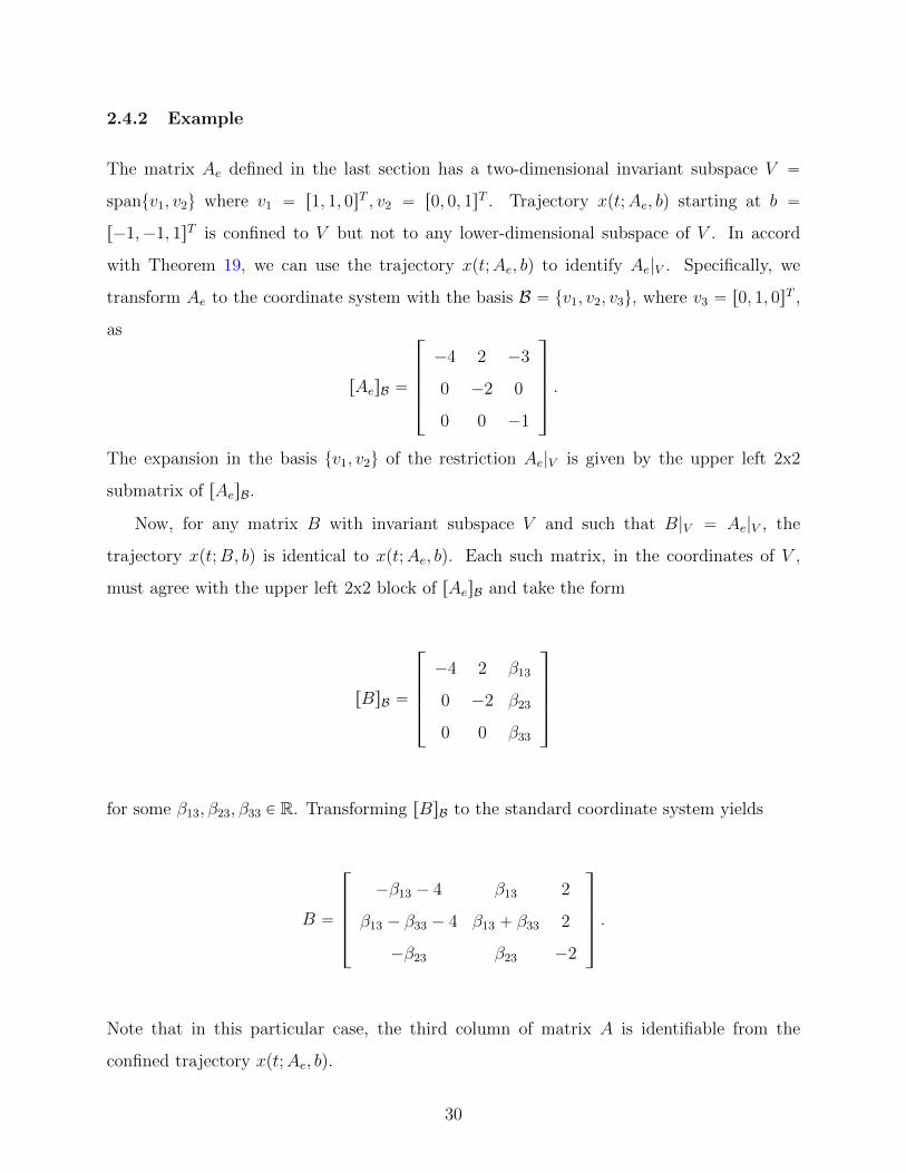
2.4.2 Example
The matrix Ae defined in the last section has a two-dimensional invariant subspace V “
spantv1, v2u where v1 “ r1, 1, 0sT , v2 “ r0, 0, 1sT . Trajectory xpt;Ae, bq starting at b “
r´1,´1, 1sT is confined to V but not to any lower-dimensional subspace of V . In accord
with Theorem 19, we can use the trajectory xpt;Ae, bq to identify Ae|V . Specifically, we
transform Ae to the coordinate system with the basis B “ tv1, v2, v3u, where v3 “ r0, 1, 0sT ,
as
rAesB “
»
—
—
—
–
´4 2 ´3
0 ´2 0
0 0 ´1
fi
ffi
ffi
ffi
fl
.
The expansion in the basis tv1, v2u of the restriction Ae|V is given by the upper left 2x2
submatrix of rAesB.
Now, for any matrix B with invariant subspace V and such that B|V “ Ae|V , the
trajectory xpt;B, bq is identical to xpt;Ae, bq. Each such matrix, in the coordinates of V ,
must agree with the upper left 2x2 block of rAesB and take the form
rBsB “
»
—
—
—
–
´4 2 β13
0 ´2 β23
0 0 β33
fi
ffi
ffi
ffi
fl
for some β13, β23, β33 P R. Transforming rBsB to the standard coordinate system yields
B “
»
—
—
—
–
´β13 ´ 4 β13 2
β13 ´ β33 ´ 4 β13 ` β33 2
´β23 β23 ´2
fi
ffi
ffi
ffi
fl
.
Note that in this particular case, the third column of matrix A is identifiable from the
confined trajectory xpt;Ae, bq.
30
2.5 SYSTEMS THAT ARE LINEAR IN PARAMETERS
2.5.1 Analysis
Consider now a nonlinear dynamical system that depends linearly on parameters and has
only its initial condition as a control:
9xptq “ Afpxptqq
xp0q “ b.(2.8)
In equation (2.8), xptq P Rn is the state of the system at time t, the system parameters
are the entries of the coefficient matrix A P Rnxm, b P Rn is the initial condition, and
f “ pf1, ..., fmq : Rn Ñ Rm, where fj are functions that are locally Lipschitz continuous in x.
The initial condition b determines the trajectory xpt;A, bq of the system (2.8) for any given
A. A definition of identifiability, analogous to Definition 1, can be stated as follows:
Definition 20. Model (2.8) is identifiable in Ω Ď Rnˆm if and only if for all A,B P Ω, A ‰
B, there exists b P Rn such that xp¨;A, bq ‰ xp¨;B, bq.
Recall that for the linear model (2.3), Theorem 2 implies identifiability in Rnˆn. Such
general identifiability, however, does not hold for systems that are linear in parameters.
Instead, we can obtain a necessary condition for identifiability of the model (2.8) using
the properties of the map f . We first introduce F , the largest linear subspace of Rm that
contains the range of f , as F “ spantfpxq|x P Rnu Ď Rm. The dimension of F determines
the identifiability of the model (2.8) as follows:
Theorem 21. If dimF ă m, then model (2.8) is not identifiable in Rnˆm.
Proof. Assume dimF “ r ă m. Let tv1, ..., vru be a basis for F . Complete tv1, ..., vru to
a basis tv1, ..., vr, vr`1, ..., vmu of Rm and let V “ rv1 | ... | vms. For fixed A P Rnˆm, choose
C P Rnˆpm´rq such that C ‰ rAvr`1 | ... |Avms and let D “ rAv1 | ... |Avr |Cs. Finally, let
B “ DV ´1. This procedure yields B P Rnˆm such that (i) Avj “ Bvj, j “ 1, .., r and (ii)
Avj ‰ Bvj for some j P tr ` 1, ...,mu. Since (i) implies that Afpxq “ Bfpxq @x P Rn, the
trajectories xpt;A, bq and xpt;B, bq of the model (2.8) are identical for any initial condition
b P Rn, yet (ii) implies that B ‰ A. Hence, the model (2.8) is not identifiable in Rnˆm.
31
One of the main results for linear systems described in Section 2.3 was Theorem 13,
which provides a connection between the uniqueness of the parameters of a model (2.3) and
the confinement of the orbit of that model. Interestingly, a similar result can be shown for
model (2.8), but here, parameter uniqueness is instead linked to the geometric structure of
the image of the orbit of the model in the flux space. Let φpA, bq “ tfpxpt;A, bqq | t P Ru be
a curve in Rm that represents the image under the map f of the orbit γpA, bq of the model
(2.8).
Theorem 22. There exists no B P Rnˆm with A ‰ B such that xp¨;A, bq “ xp¨;B, bq if and
only if φpA, bq is not confined to a proper subspace of Rm.
Proof. To prove the reverse implication, suppose that φpA, bq is not confined to a proper
subspace of Rm. Then one can find the matrix A uniquely as follows: Since φpA, bq is
not confined, one can choose m distinct time points t1, ..., tm, such that the matrix F “
rfpxpt1qq | ... | fpxptmqqs is invertible. From knowledge of the trajectory, one knows 9xpt1q, . . . ,
9xptmq. Appending this information into a matrix yields the linear equation r 9xpt1q | ... | 9xptmqs “
A rfpxpt1qq | ... | fpxptmqqs “ AF , which has a unique solution A “ r 9xpt1q | ... | 9xptmqsF´1.
Therefore there is no other matrix B that would produce a trajectory identical to A.
The forward direction is proven by contrapositive utilizing an argument similar to the
one used in the proof of Theorem 21. Assume that φpA, bq is confined to a proper sub-
space of Rm and define Fγ “spantfpxpt, A, bqq, t P r0,8qu. By the confinement of φpA, bq,
dimFγ “ r ă m. Let V “ tv1, ..., vru be a basis for Fγ. Complete V to a basis of
Rm, V “ tv1, ..., vr, vr`1, ..., vmu. Construct B P Rnˆm such that Avj “ Bvj, j “ 1, .., r, but
Avj ‰ Bvj for some j P tr ` 1, ...,mu (as in the previous proof). With this construction,
A ‰ B, but, Afpxq “ Bfpxq @x P Rn, and hence xpt;A, bq “ xpt;B, bq.
As in the linear case, this theorem is a statement about identifiability of the model from
a single trajectory. In fact, since the linear model (2.3) is a special case of the nonlinear
model (2.8) with f being the identity map, Theorem 13 is a special case of Theorem 22. In
that case, the confinement of the orbit image φpA, bq in the flux space is equivalent to the
confinement of the orbit γpA, bq of the trajectory.
32

Figure 7: Confinement of φpA, bq in the flux space.
2.5.2 Examples
As an illustrative example, consider the system,
9x “ a11x` a12xy ` a13y
9y “ a21x` a22xy ` a23y(2.9)
System (2.9) is linear in parameters and can be represented in the form of model (2.8)
with
A “
»
–
a11 a12 a13
a21 a22 a23
fi
fl
and fpx, yq “ rx, xy, ysT . For the matrix
A “
»
–
´2 1 ´2
´1 1 ´3
fi
fl
and initial condition b “ r1, 1sT , φpA, bq is confined to a proper subspace of R3, as shown
in figure (7). Theorem 22 implies that there exists a matrix B P R2ˆ3 with A ‰ B
such that xpt;A, bq “ xpt;B, bq. One can construct B using the procedure described in
the proof of the theorem. Since xptq “ yptq for the solution of the IVP, we have Fγ “
33

spantpx, x2, xqT |x P Ru. Thus tp1, 0, 1qT , p0, 1, 0qT u is a basis for Fγ. Complete this basis to
tv1, v2, v3u “ tp1, 0, 1qT , p0, 1, 0qT , p1, 0,´1qT u, a basis of R3. Let
D “ rAv1 |Av2 |ws “
»
–
´4 1
´4 1w
fi
fl
such that w ‰ Av3 “ r0, 2sT . For example, let
D “
»
–
´4 1 ´2
´4 1 ´6
fi
fl .
Then
B “ Drv1 | v2 | v3s´1“
»
–
´3 1 ´1
´5 1 1
fi
fl
is one such example.
Another example is provided by the Lotka-Volterra model of competing species [21, 66],
9x “ xp1´ ax´ cyq
9y “ yp1´ ay ´ cxq.(2.10)
Model (2.10) is linear in parameters with
A “
»
–
1 ´a ´c 0 0
0 0 ´c 1 ´a
fi
fl
and fpx, yq “ rx, x2, xy, y, y2sT .
For any initial condition of the form b “ rx0, x0sT , the trajectory of the system obeys
xptq “ yptq and depends on the sum a`c but not the individual values of the parameters a, c.
This is consistent with Theorem 22, which concludes that since fpx, xq “ rx, x2, x2, x, x2sT
and φpA, bq is confined to a proper subspace of R5, the parameter matrix which yields this
trajectory is not unique, and therefore model (2.10) is not identifiable in R2ˆ5.
34
2.6 DISCRETE DATA
In practical applications, one does not typically have knowledge of a full trajectory of
the system, but rather a sample of discrete data points that lie on a trajectory, possi-
bly perturbed by measurement noise. Suppose for now that we have m accurate data
points x0, x1, . . . , xm´1 in Rn that lie on the trajectory of the model (2.3), defined as
xk “ xptk;A, bq, k “ 0, 1, . . . ,m ´ 1, where t0, t1, . . . , tm´1 are distinct time points. Non-
confinement of the orbit γpA, bq “ txpt;A, bq : t P Ru is obviously determined by the dimen-
sion of the span of the data vectors.:
Lemma 23. Orbit γpA, bq is not confined to a proper subspace of Rn if and only if there
exist t0, t2, . . . , tn´1 such that x0, x2, . . . , xn´1 are linearly independent.
Note that the confinement of an orbit cannot be established from a fixed, finite data
set. For example, in a two-dimensional system, the available data may lie in a straight line,
but the underlying solution may be a spiral, which is not a confined orbit. Model (2.3)
is identifiable from a full trajectory in this example, since the corresponding orbit is not
confined to a proper subspace.
It now remains to show how the parameter matrix A is determined from the data. The
parameter matrix A can be computed explicitly without the need for optimization from n`1
data points which are uniformly spaced in time. Let x0, . . . , xn be such that xk “ xptk;A, bq
for each k “ 0, . . . , n, with tk`1 ´ tk “ ∆t for all k “ 0, . . . , n ´ 1. Assume that every
collection of n of the data points are linearly independent. Let Φp∆tq denote the principal
matrix solution of model (2.3) and let X0 and X1 denote the matrices rx0 |x1 | ... |xn´1s and
rx1 |x2 | ... |xns, respectively. The principal matrix solution provides a relation between the
data given by Φp∆tqxk “ xk`1, thus Φp∆tqX0 “ X1. Without loss of generality, we can let
∆t “ 1 and define Φ “ Φp1q. Then, by the invertibility of X0 we find that,
Φ “ X1pX0q´1. (2.11)
In theory, the matrix A can be computed by taking the matrix logarithm of Φ, since Φ “ eA.
It is important to note, however, that the logarithm of a matrix does not always exist, and if
35
it does, it is not necessarily unique. Requirements for the existence of a real matrix logarithm
are given in the following theorem [17].
Theorem 24. Let Φ be a real square matrix. Then there exists a real solution A to the
equation Φ “ eA if and only if Φ is nonsingular and each Jordan block of Φ belonging to a
negative eigenvalue occurs an even number of times.
In our case, Φ “ X1pX0q´1 is nonsingular due to the linear independence of the data.
The second condition of Theorem 24 is satisfied trivially if x0, x2, . . . , xn are indeed discrete
points on a trajectory of the linear model (2.3). More importantly, uniqueness of the matrix
logarithm, which is directly related to the identifiability of the model (2.3), is addressed in
the following theorem [17].
Theorem 25. Let Φ be a real square matrix. Then there exists a unique real solution A to
the equation Φ “ eA if and only if all the eigenvalues of Φ are positive real and no Jordan
block of Φ belonging to any eigenvalue appears more than once.
Given the data x0, x2, . . . , xn, the matrix logarithm yields a unique corresponding pa-
rameter matrix A if and only if Φ, defined using (2.11), satisfies the hypotheses of Theorem
25. We have established earlier (in Theorem 15) that model (2.3) can be identified from
some initial condition b if and only if A has only one Jordan block for each of its eigenvalues.
If A satisfies this requirement and has real eigenvalues, then Φ has positive eigenvalues and
has one Jordan block for each of them and hence satisfies the hypotheses of Theorem 25. We
can then conclude that model (2.3) is identifiable from the data x0, x1, . . . , xn. If, however,
A has one Jordan block for each of its eigenvalues and has complex eigenvalues, then Φ
has a negative eigenvalue and a pair of Jordan blocks associated to each pair of complex
eigenvalues of A. For example,
A “
»
–
0 π
´π 0
fi
fl
has eigenvalues ˘πi and has no repeated Jordan blocks, yet
eA “
»
–
´1 0
0 ´1
fi
fl
36

x
y
r = 0
r = 1
r = −1
(a)
0 1 2 3−5
0
5
t
x(t
)
r = 0
r = 1
r = −1
(b)
Figure 8: paq Plot of the orbits for Ar with r “ 0, 1,´1, pbq Plot of the x component of the
trajectory. Each of the three distinct systems satisfy the data.
with a repeated Jordan block and negative eigenvalues. In such a case, Theorem 25 implies
that one can find a matrix B ‰ A such that eB “ Φ “ eA. Although the trajectories
xpt;A, x0q and xpt;B, x0qmust necessarily differ (since the model with matrix A is identifiable
from the full trajectory xpt;A, x0q), the data obtained from these trajectories for the same
set of time points tt0, t2, . . . , tnu are identical. Thus, we have the following observation.
Corollary 26. The model (2.3) with matrix A that has a pair of complex eigenvalues is not
identifiable from any set of data x0, x2, . . . , xn that are uniformly spaced in t.
Figure 8 illustrates the non-identifiability that arises with complex eigenvalues in the
case of discrete data for 2x2 linear systems. In this example, the solution to the system with
parameter matrix
Ar “
»
–
´32 ´4
4 ´32
fi
fl` 2πr
»
–
0 ´1
1 0
fi
fl
will satisfy the data for any integer value of r. The solutions shown in Figure 8 are for the
cases r “ 0, 1, and ´1.
The extension of the above computation to the model (2.8) is simple, provided one can
measure not only the values x1, x2, . . . , xm of the variables at t1, t2, . . . , tm, but also their
37

rates of change y1, y2, . . . , ym, where yk “ dxpt;A, bqdt|t“tk . Just as in the proof of Theorem
22, if fpx1q, fpx2q, . . . , fpxnq are linearly independent (and hence φpA, bq is not confined to
a proper subspace), then the unique parameter matrix that yields this data is given by
A “ Y F´1 (2.12)
where Y “ ry1 | . . . | yms and F “ rfpx1q | . . . | fpxmqs.
The computations outlined above are valuable not only because they offer direct methods
for computing the parameter matrix A that do not rely on minimization of an error function,
but also because they can be used to provide insight into the sensitivity of A to the data.
Since both computations are based on linear algebraic operations, one can use the tools of
numerical analysis to determine the conditioning of the problem (see, e.g., [83]). In the case of
the linear model (2.3), equation (2.11) implies that the problem of computing Φ has condition
number κpX0q “ X0pX0q´1, and indeed one can compute that any perturbations of the
data (δX0 of X0 and δX1 of X1) induce a perturbation δΦ of Φ that obeys
δΦ
Φď κpX0q
ˆ
δX0
X0`δX1
X1
˙
(2.13)
where . is any norm of choice. Note that if . is the Euclidean norm .2, then κpX0q
equals the ratio of the largest to the smallest singular values of X0. It follows that the closer
are the data vectors x0, x1, . . . , xn´1 (i.e., the columns of X0) to being linearly dependent,
the more ill-conditioned is the inverse problem.
Likewise, in the case of the model (2.8), equation (2.12) implies that the problem of
computing A has the condition number κpF q “ F F´1, and hence any perturbations δF
and δY induce a perturbation δA that obeys
δA
Aď κpF q
ˆ
δF
F `δY
Y
˙
. (2.14)
Again, the closer are the vectors fpx1q, fpx2q, . . . , fpxmq (i.e., the columns of F ) to being
linearly dependent, the more ill-conditioned is the inverse problem.
The observations made at the end of this section indicate that the highest accuracy in
the inverse problem (and hence the lowest sensitivity to measurement errors) can be achieved
by selecting data so as to minimize the condition number of the data matrix. This result
38
has an important practical implication: although the results in Sections 2.3 and 2.5 indicate
that for an identifiable model any infinitesimally small portion of a trajectory is sufficient
to identify the parameter matrix, in any practical situation a small segment of trajectory
will have a nearly linear orbit and hence any selection of data from that segment will yield a
data matrix with high condition number. Thus, in order to minimize the condition number,
one must have a sufficiently large portion of the trajectory that explores all dimensions of
the underlying space.
2.7 CONCLUSIONS
In this chapter, for both linear and nonlinear dynamical systems, we have derived necessary
and sufficient conditions for identifiability of parameters from a single trajectory based solely
on the geometry of the trajectory or the geometry of an image of the trajectory. Furthermore,
we have shown that an improved accuracy of parameter estimation can result when the tra-
jectory deviates farther from being confined. These results have a practical utility since the
criterion can be applied using only what is known about the trajectory, without any knowl-
edge of the model parameters. Additional results for linear systems include a link between
identifiability from single trajectory with initial condition b and the linear independence of
tb, Ab, ..., An´1bu, several characterizations of the linear independence of tb, Ab, ..., An´1bu in-
cluding a condition on the Jordan form of A, and the result that unconditional identifiability
cannot occur outside of R2nˆ2n. Finally, we addressed the question of explicitly computing
model parameter values from a discrete collection of data points.
There are several directions for possible extension of the results in this chapter. First,
our results imply that discrete data contained within a lower-dimensional subspace of the
full state space will not yield identifiability of an underlying system. Such data may arise,
however, from particular samplings of a trajectory that is not confined in this way. The
derivation of more general identifiability conditions from discrete data remains for future
exploration. Second, the condition C “ I is highly restrictive, because in real scenarios not
all variables of the system may be observable. We have shown that when C is not of full
39

rank, then confinement of an orbit to an invariant subspace of dimension not greater than
the rank of C can yield partial identifiability of the parameter matrix. A natural extension
of the present study would be to investigate if there are ways to enhance the practical
applicability of this result or to obtain more general identifiability results in this case. A
third direction for future study would be the consideration of general nonlinear systems. We
have shown that identifiability conditions based on confinement can be derived for systems
that feature linearity in parameters, regardless of whether the dynamics is linear or nonlinear.
For nonlinear dynamical systems lacking this form of parameter dependence, the assessment
of identifiability will likely require new ideas. The prospects for addressing this problem
using linearization about trajectories appear to be limited, based on our observations about
sensitivity associated with parameter estimation from small segments of trajectories. A final
direction to consider is the identifiability of systems that are linear or linear in parameters
with time-dependent parameter matrices. Our methods would likely be useful for systems
with rather trivial time-dependence, such as piecewise constant parameter matrices, where
switching times between different constant values are known and full solution trajectories
are available, but handling more general time-dependence appears to be a difficult problem.
These and other related topics represent important directions for follow-up studies.
In the next chapter, we will continue to look at the case of discrete single trajectory data.
Moving beyond the setting of error free data, we will investigate properties of the inverse
solution in the presence of uncertainty in the data.
40
3.0 ROBUSTNESS OF SOLUTIONS OF THE INVERSE PROBLEM FOR
LINEAR DYNAMICAL SYSTEMS WITH UNCERTAIN DATA
3.1 INTRODUCTION
A fundamental problem in modeling temporally evolving systems is the determination of
model parameter values from experimental observations collected at specific time points.
Since models can be viewed as forward mappings from sets of parameter values to time-
dependent states of model variables, the problem of parameter estimation is often referred
to as an inverse problem. Although parameter estimation has received significant attention
in the literature, certain fundamental questions about the inverse problem still remain open.
Solving the inverse problem becomes even more challenging in the presence of uncertainty
in experimental measurements, as may arise due to measurement errors and fluctuations in
system components. The overall goal of this chapter is to derive estimates of the degree
of uncertainty in data to which properties of the inverse problem, such as existence and
uniqueness of solutions, are robust.
We start by addressing fundamental issues of existence and uniqueness of solutions to the
inverse problem based on a discrete collection of linearly independent data points assumed to
be known without uncertainty, before turning to the uncertain case. We focus our analysis
on linear models, which are prevalent in the study of many important applications including
pharmacokinetics, linear response theory for mechanical and electronic systems, continuous
time Markov chain probabilistic models, and near-equilibrium responses of nonlinear systems
[11, 31, 3, 73]. In addition to their applicability, linear systems are convenient because in the
linear case, there is an explicit structure of the associated forward solution map that can be
exploited. Furthermore, we mostly consider data points that are equally spaced in time, as
41
may be obtained from experiments with regimented data collection schedules and for which
it may be possible to explicitly solve for the linear system parameter matrix. Despite these
advantages, the inverse problem is nontrivial because the solution to a linear dynamical
system depends nonlinearly on its parameters.
Specifically, in Section 3.2, we begin by considering data with no uncertainty, where
classical results on matrix logarithms yield necessary and sufficient conditions for the data
to specify a unique parameter matrix A that solves the inverse problem. Contrary to our
expectations, we find that the existence of model parameters corresponding to given data is
guaranteed only for a restricted subset of potential data sets and that there is only a limited
region in data space that yields a unique set of parameters. Subsequently, we explore how
uncertainty in the data impacts the existence and uniqueness of A. In Section 3.3, we
provide conditions that ensure that existence or uniqueness of the inverse problem solution
is guaranteed to hold in an open neighborhood of data, and we make use of a convenient
transformation to better characterize regions in which A is unique. These steps prepare us
for Section 3.4, where we present the main results of the chapter, consisting of analytical
and numerical estimates of the maximum uncertainty in the data under which the properties
of the inverse problem are certain to be preserved. Examples for 2-dimensional systems are
shown in Section 3.5, where we first define regions in data space for which the solution
to the inverse problem has various properties and then illustrate bounds on the maximal
permissible uncertainty for those properties. Finally, in Section 3.6, we briefly remark on
the case of non-equally-spaced data points, and we conclude with a discussion in Section 3.7,
which includes some comments on open directions and related work in the past literature.
3.2 DEFINITIONS AND PRELIMINARIES
As in Chapter 2, we consider the model defined as a finite-dimensional linear dynamical
system; recall equation (2.3):
9xptq “ Axptq
xp0q “ b.
42

In equation (2.3), xptq P Rn is the state of the system at time t, the system parameters are
the entries of the coefficient matrix A P Rnˆn and b P Rn is the initial condition. For clarity
of exposition we will refer to the entire matrix A as the parameter A. We shall define the
parameter space P as the set of all parameters A and initial conditions b.
For a fixed A, system (2.3) has a well defined solution, or trajectory, given by xpt;A, bq “
Φptqb, where Φptq “ eAt is the principal matrix solution. The data representing the system
is a set of observations of the trajectory values. We assume that data for all of the state
variables is available and denote by D the data space consisting of a set of pn ` 1q-tuples
d “ px0, x1, x2, . . . , xnq of points xj P Rn. Each such d will be referred to as a data set and
each xj as a data point. Sampling the trajectory xpt;A, bq at equally spaced times (without
loss of generality ∆t “ 1) yields an element of D, namely a data set composed of the specific
data points xj “ xpj; A, bq P Rn, j “ 0, 1, . . . , n; non-uniformly spaced data are discussed
in Section 3.6. We use solution map to refer to the map F : P Ñ D from parameter space
to data space defined as F pA, bq “ px0, x1, x2, . . . , xnq for this choice of txju sampled from
xpt;A, bq. From the definition of xj, it is immediately clear that b “ x0 and thus, we focus
on the problem of determining the parameter A. The inverse problem is then the problem
of inverting the map F to find F´1pdq (i.e., A such that F pA, b “ x0q “ d) for a given data
set d. If the data set d is obtained from experimental measurements or some other outside
source, then this problem may or may not have a solution.
We set out to derive necessary and sufficient conditions that a data set d P D must satisfy
so that there exists a unique real matrix A for which the dynamical system (2.3) produces
data d (i.e., so that d “ F pA, bq). These conditions define a subset of the data space on
which the inverse map F´1 is well defined. Given a uniformly spaced data set d P D, one can
attempt to solve the inverse problem as presented in Section 2.6. We review the constructs
here, as this notation is referenced several times throughout this chapter. Denote by X0
and X1 the n ˆ n matrices rx0 | . . . |xn´1s and rx1 | . . . |xns, respectively. The principal
matrix solution provides a relation between the data points; letting Φ :“ Φp1q “ eA, we have
xj`1 “ Φxj, which implies that X1 “ ΦX0 and hence Φ “ X1X´10 . All that remains is to
find A as the matrix logarithm of Φ. Thus, from an operational standpoint, the map F´1 is a
composition of two nonlinear maps: (i) The map G : D Ñ Rnˆn defined by Gpdq “ Φ, which
43

is defined (and continuous) at all points d such that x0, . . . , xn´1 are linearly independent
(i.e. wherever X´10 exists), and (ii) the matrix logarithm map, denoted here as L : Rnˆn Ñ P
and defined as A “ LpeAq. Hence, F´1 “ L ˝ G is well defined if (i) X0 is invertible, (ii)
the matrix logarithm of Φ exists, and (iii) the matrix logarithm of Φ is unique. The case
when condition (i) fails was studied extensively in Chapter 2; in that case the system (2.3)
generating the data d either does not exist or is not identifiable. Conditions (ii) and (iii) can
be addressed with the help of theorems 24 and 25 by Culver [17], presented in Section 2.6,
which characterize the existence and uniqueness of a real matrix logarithm.
We note that even when a matrix logarithm exists, there are still issues with how to
compute it. Numerical methods for computing the logarithm of a matrix are discussed in
[37, 14, 1].
3.3 EXISTENCE AND UNIQUENESS OF THE INVERSE IN N
DIMENSIONS
As will become clear shortly, Theorems 24 and 25 identify matrices Φ that are not robust
in the sense that they form a set of zero measure. Since we aim to discuss the properties of
inverse problem solutions for uncertain data, such as data that is perturbed due to noise, it
makes sense to determine conditions that ensure that a given matrix Φ is inside an open set
of matrices with particular existence or uniqueness properties.
3.3.1 Inverse problems on open sets
We now state and prove three corollaries of Theorems 24 and 25 that are useful for considering
uncertain data and, as it turns out, avoid the conditions on Jordan blocks that can become
overly cumbersome for practical use in n dimensions. The first corollary characterizes open
sets of matrices that have real logarithms, the second corollary characterizes open sets of
matrices that have unique real logarithms, and the third corollary characterizes open sets of
matrices that do not have real logarithms.
44

Corollary 27. (to Theorem 24) Let Φ˚ be an n ˆ n real matrix. The following statements
are equivalent:
(a) There exists an open set U Ă Rnˆn containing Φ˚ such that for any Φ P U the equation
Φ “ eA has an nˆ n real solution A.
(b) Φ˚ has only positive real or complex eigenvalues.
Proof. Suppose that Φ˚ P Rnˆn has only positive real or complex eigenvalues. Then the
result follows immediately by Theorem 24 and the continuous dependence of eigenvalues on
matrix entries.
For the converse, suppose that Φ˚ P Rnˆn has a real matrix logarithm, i.e., Φ˚ “ eA
where A is nˆ n real matrix. By Theorem 24, either Φ˚ satisfies pbq, or Φ˚ has at least one
negative eigenvalue and the corresponding Jordan block occurs an even number of times.
We now show that the second alternative contradicts the existence of the open set U . To
this end, let Φ˚ “ QJQ´1, where
J “
»
—
—
—
–
J1 0
0 J2
. . .
fi
ffi
ffi
ffi
fl
(3.1)
is a Jordan canonical form of Φ˚ with J1 a Jordan block corresponding to a negative eigen-
value. Let B “ QKQ´1 where,
K “
»
–
aI 0
0 0
fi
fl ,
with a P R and I the identity matrix of the same size as J1. Then for every sufficiently small
nonzero a, Φ`B has a negative eigenvalue for which the corresponding Jordan block occurs
exactly once and hence there is no real A such that Φ`B “ eA.
Corollary 28. (to Theorem 25) Let Φ˚ be nˆ n real matrix. The following statements are
equivalent:
(a) There exists an open set U Ă Rnˆn containing Φ˚ such that for any Φ in U the equation
Φ “ eA has a unique nˆ n real solution A.
(b) Φ˚ has n distinct positive real eigenvalues.
45

Proof. The proof is similar to the previous one. Condition (b) implies condition (a) based
on Theorem 25 and continuity. For the converse, suppose that Φ˚ P Rnˆn has a unique real
matrix logarithm, i.e., there is a unique A P Rnˆn such that Φ˚ “ eA, and Φ˚ is in the
interior of an open set of such matrices. By Theorem 25, Φ˚ has positive real eigenvalues
and no Jordan block appears more than once. There can be more than one Jordan block
for the same eigenvalue but those Jordan blocks must be of different sizes. We can write
Φ˚ “ QJQ´1 where J is the Jordan canonical form of Φ˚ as defined in (3.1) and Ji are
ordered in size from largest to smallest, such that no two Ji are the same.
Suppose now that the largest Jordan block, J1, is not a 1 ˆ 1 matrix. Let pJptq be the
characteristic polynomial of J , i.e., pJptq “śk
i“1pλi ´ tqdi where λi are all real positive and
d1 ě 2. Let B “ QKQ´1 where K is an n ˆ n matrix with all zero entries except L12 “ a,
L21 “ ´a. Then, for every a ą 0, J “ J ` K has entries J12 “ 1 ` a, J21 “ ´a, which
implies that J has characteristic polynomial
pJptq ““
pλ1 ´ tq2` ap1` aq
‰
pλ1 ´ tqd1´2
kź
i“2
pλi ´ tqdi
with two complex roots. It follows that Φ˚ ` B “ eA does not have a unique real solution
A for a ą 0, which contradicts the assumption that A is unique for each Φ in an open set
containing Φ˚. Thus, all Jordan blocks Ji are of size 1 and furthermore, since no two Ji can
be the same, Φ˚ has n distinct eigenvalues.
Statements similar to Corollaries 27, 28 can be made to establish the existence of open
sets of matrices with other properties. An example follows.
Corollary 29. (to Theorem 24) Let Φ˚ be nˆ n real matrix. The following statements are
equivalent:
(a) There exists an open set U Ă Rnˆn containing Φ˚ such that for each Φ P U the equation
Φ “ eA does not have an nˆ n real solution A.
(b) Φ˚ has at least one negative eigenvalue of odd multiplicity.
46
Proof. Suppose that Φ˚ P Rnˆn has at least one negative eigenvalue of odd multiplicity.
Then, there is at least one Jordan block associated to it that occurs an odd number of times
and hence, by Theorem 24, there is no A P Rnˆn such that Φ˚ “ eA. Moreover, there exists
an open neighborhood of Φ˚ for which there remains at least one negative eigenvalue of odd
multiplicity. 1
For the converse, suppose that there exists an open set U Ă Rnˆn containing Φ˚ such
that for each Φ P U the equation Φ “ eA does not have an n ˆ n real solution A. Since
Φ˚ “ eA has no real solution, by Theorem 24, either Φ˚ is singular, or there is a negative
eigenvalue of Φ˚ which belongs to a Jordan block that appears an odd number of times, or
both.
If Φ˚ is singular with no Jordan block associated to a negative eigenvalue occurring an
odd number of times, then in every neighborhood of Φ˚ there exists a Φ which is nonsingular
with the same condition on Jordan blocks, and Φ “ eA will have a real solution A. This
contradicts the existence of U .
Thus, there is at least one negative eigenvalue of Φ˚ for which a Jordan block repeats an
odd number of times. Denote these negative eigenvalues by λ1, . . . λr, r ě 1. Let mλi be the
multiplicity of λi.
Suppose that all mλi are even. Let Φ˚ “ QJQ´1 where J is the Jordan canonical form of
Φ˚ as defined in (3.1), let Jλ11 , Jλ1
2 , . . . , Jλ1k denote all of the Jordan blocks associated to λ1
(the blocks may have the same size), and denote by J1 the block-diagonal matrix comprised
of Jλ11 , Jλ1
2 , . . . , Jλ1k .
For i “ 1, ..., k define W λ1i to be a block-diagonal matrix of the same dimension as Jλ1
i
comprised of K, where
K “
»
–
0 a
´a 0
fi
fl
for some a ą 0. If the dimension of Jλ1i is even and equal to 2s, then W λ1
i is comprised of ex-
actly s blocks K, the characteristic polynomial of Jλ1i `W
λ1i is pptq “ rpλ1 ´ tq
2 ` ap1` aqss
and, since a ą 0, Jλ1i `W λ1
i has only complex eigenvalues.
1A perturbation may split it into a collection of distinct negative eigenvalues of various multiplicitiesand/or complex pairs, but at least one negative eigenvalue with odd multiplicity will remain.
47
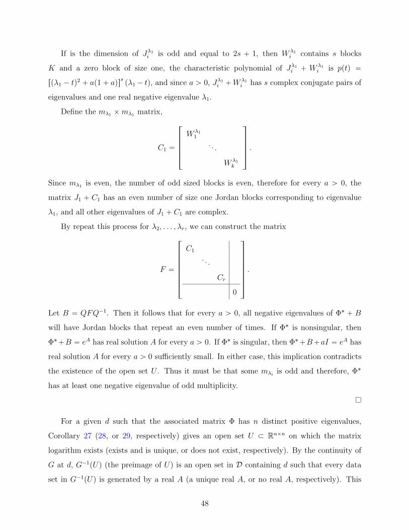
If is the dimension of Jλ1i is odd and equal to 2s ` 1, then W λ1
i contains s blocks
K and a zero block of size one, the characteristic polynomial of Jλ1i ` W λ1
i is pptq “
rpλ1 ´ tq2 ` ap1` aqs
spλ1´ tq, and since a ą 0, Jλ1
i `W λ1i has s complex conjugate pairs of
eigenvalues and one real negative eigenvalue λ1.
Define the mλ1 ˆmλ1 matrix,
C1 “
»
—
—
—
–
W λ11
. . .
W λ1k
fi
ffi
ffi
ffi
fl
.
Since mλ1 is even, the number of odd sized blocks is even, therefore for every a ą 0, the
matrix J1 ` C1 has an even number of size one Jordan blocks corresponding to eigenvalue
λ1, and all other eigenvalues of J1 ` C1 are complex.
By repeat this process for λ2, . . . , λr, we can construct the matrix
F “
»
—
—
—
—
—
—
–
C1
. . .
Cr
0
fi
ffi
ffi
ffi
ffi
ffi
ffi
fl
.
Let B “ QFQ´1. Then it follows that for every a ą 0, all negative eigenvalues of Φ˚ ` B
will have Jordan blocks that repeat an even number of times. If Φ˚ is nonsingular, then
Φ˚`B “ eA has real solution A for every a ą 0. If Φ˚ is singular, then Φ˚`B`aI “ eA has
real solution A for every a ą 0 sufficiently small. In either case, this implication contradicts
the existence of the open set U . Thus it must be that some mλi is odd and therefore, Φ˚
has at least one negative eigenvalue of odd multiplicity.
For a given d such that the associated matrix Φ has n distinct positive eigenvalues,
Corollary 27 (28, or 29, respectively) gives an open set U Ă Rnˆn on which the matrix
logarithm exists (exists and is unique, or does not exist, respectively). By the continuity of
G at d, G´1pUq (the preimage of U) is an open set in D containing d such that every data
set in G´1pUq is generated by a real A (a unique real A, or no real A, respectively). This
48
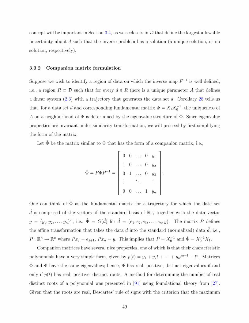
concept will be important in Section 3.4, as we seek sets in D that define the largest allowable
uncertainty about d such that the inverse problem has a solution (a unique solution, or no
solution, respectively).
3.3.2 Companion matrix formulation
Suppose we wish to identify a region of data on which the inverse map F´1 is well defined,
i.e., a region R Ă D such that for every d P R there is a unique parameter A that defines
a linear system (2.3) with a trajectory that generates the data set d. Corollary 28 tells us
that, for a data set d and corresponding fundamental matrix Φ “ X1X´10 , the uniqueness of
A on a neighborhood of Φ is determined by the eigenvalue structure of Φ. Since eigenvalue
properties are invariant under similarity transformation, we will proceed by first simplifying
the form of the matrix.
Let Φ be the matrix similar to Φ that has the form of a companion matrix, i.e.,
Φ “ PΦP´1“
»
—
—
—
—
—
—
—
—
—
–
0 0 . . . 0 y1
1 0 . . . 0 y2
0 1 . . . 0 y3
.... . .
...
0 0 . . . 1 yn
fi
ffi
ffi
ffi
ffi
ffi
ffi
ffi
ffi
ffi
fl
.
One can think of Φ as the fundamental matrix for a trajectory for which the data set
d is comprised of the vectors of the standard basis of Rn, together with the data vector
y “ py1, y2, . . . , ynqT , i.e., Φ “ Gpdq for d “ pe1, e2, e3, . . . , en, yq. The matrix P defines
the affine transformation that takes the data d into the standard (normalized) data d, i.e.,
P : Rn Ñ Rn where Pxj “ ej`1, Pxn “ y. This implies that P “ X´10 and Φ “ X´1
0 X1.
Companion matrices have several nice properties, one of which is that their characteristic
polynomials have a very simple form, given by pptq “ y1 ` y2t` ¨ ¨ ¨ ` yntn´1 ´ tn. Matrices
Φ and Φ have the same eigenvalues; hence, Φ has real, positive, distinct eigenvalues if and
only if pptq has real, positive, distinct roots. A method for determining the number of real
distinct roots of a polynomial was presented in [91] using foundational theory from [27].
Given that the roots are real, Descartes’ rule of signs with the criterion that the maximum
49
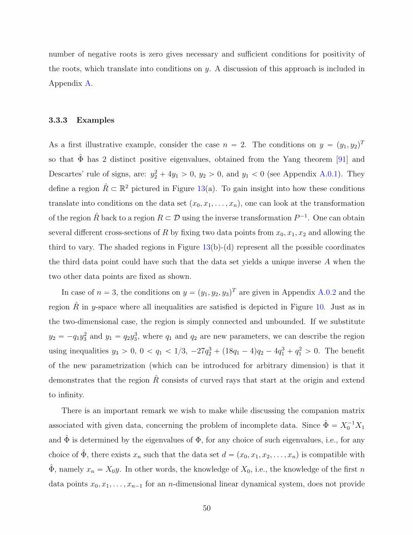
number of negative roots is zero gives necessary and sufficient conditions for positivity of
the roots, which translate into conditions on y. A discussion of this approach is included in
Appendix A.
3.3.3 Examples
As a first illustrative example, consider the case n “ 2. The conditions on y “ py1, y2qT
so that Φ has 2 distinct positive eigenvalues, obtained from the Yang theorem [91] and
Descartes’ rule of signs, are: y22 ` 4y1 ą 0, y2 ą 0, and y1 ă 0 (see Appendix A.0.1). They
define a region R Ă R2 pictured in Figure 13(a). To gain insight into how these conditions
translate into conditions on the data set px0, x1, . . . , xnq, one can look at the transformation
of the region R back to a region R Ă D using the inverse transformation P´1. One can obtain
several different cross-sections of R by fixing two data points from x0, x1, x2 and allowing the
third to vary. The shaded regions in Figure 13(b)-(d) represent all the possible coordinates
the third data point could have such that the data set yields a unique inverse A when the
two other data points are fixed as shown.
In case of n “ 3, the conditions on y “ py1, y2, y3qT are given in Appendix A.0.2 and the
region R in y-space where all inequalities are satisfied is depicted in Figure 10. Just as in
the two-dimensional case, the region is simply connected and unbounded. If we substitute
y2 “ ´q1y23 and y1 “ q2y
33, where q1 and q2 are new parameters, we can describe the region
using inequalities y3 ą 0, 0 ă q1 ă 13, ´27q32 ` p18q1 ´ 4qq2 ´ 4q3
1 ` q21 ą 0. The benefit
of the new parametrization (which can be introduced for arbitrary dimension) is that it
demonstrates that the region R consists of curved rays that start at the origin and extend
to infinity.
There is an important remark we wish to make while discussing the companion matrix
associated with given data, concerning the problem of incomplete data. Since Φ “ X´10 X1
and Φ is determined by the eigenvalues of Φ, for any choice of such eigenvalues, i.e., for any
choice of Φ, there exists xn such that the data set d “ px0, x1, x2, . . . , xnq is compatible with
Φ, namely xn “ X0y. In other words, the knowledge of X0, i.e., the knowledge of the first n
data points x0, x1, . . . , xn´1 for an n-dimensional linear dynamical system, does not provide
50
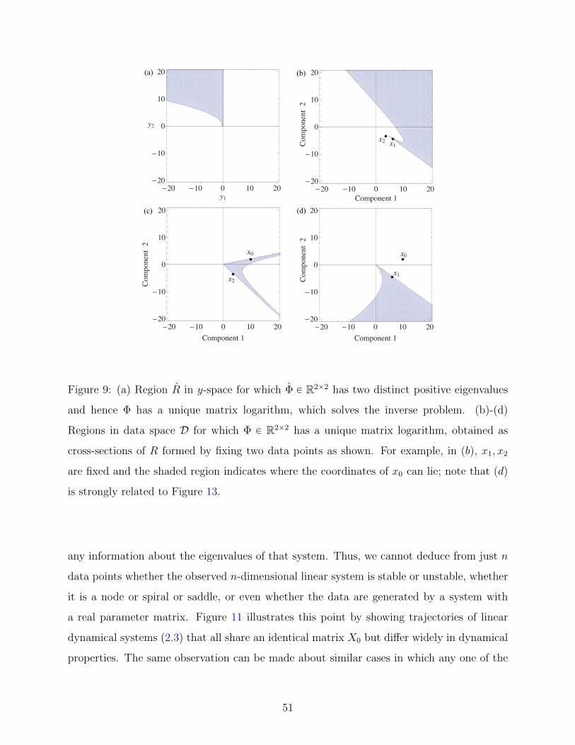
20 10 0 10 2020
10
0
10
20
y1
y2
(a)
x1x2
20 10 0 10 2020
10
0
10
20
Component 1
Component2
(b)
x0
x2
20 10 0 10 2020
10
0
10
20
Component 1
Component2
(c)
x0
x1
20 10 0 10 2020
10
0
10
20
Component 1
Component2
(d)
Figure 9: (a) Region R in y-space for which Φ P R2ˆ2 has two distinct positive eigenvalues
and hence Φ has a unique matrix logarithm, which solves the inverse problem. (b)-(d)
Regions in data space D for which Φ P R2ˆ2 has a unique matrix logarithm, obtained as
cross-sections of R formed by fixing two data points as shown. For example, in pbq, x1, x2
are fixed and the shaded region indicates where the coordinates of x0 can lie; note that pdq
is strongly related to Figure 13.
any information about the eigenvalues of that system. Thus, we cannot deduce from just n
data points whether the observed n-dimensional linear system is stable or unstable, whether
it is a node or spiral or saddle, or even whether the data are generated by a system with
a real parameter matrix. Figure 11 illustrates this point by showing trajectories of linear
dynamical systems (2.3) that all share an identical matrix X0 but differ widely in dynamical
properties. The same observation can be made about similar cases in which any one of the
51

3
2
y3
1
00-1
y2
-2-3
1
0.8
0.6
0.4
0.2
0
y1
Figure 10: Region R in y-space for which Φ P R3ˆ3 has a unique matrix logarithm.
.
n` 1 data points x0, x1, x2, . . . , xn is missing.
3.4 ANALYSIS OF UNCERTAINTY IN THE DETERMINATION AND
CHARACTERIZATION OF INVERSE
Realistic data are never exact, but are subject to uncertainty caused by measurement error,
fluctuation in experimental conditions, or variability in experimental subjects. A natural
question arises as to how large an uncertainty in the data can be tolerated without altering
the properties of the solution to the inverse problem. Several scenarios are of interest; for
example,
• The data imply that the inverse system has a stable node. What is the largest uncertainty
in the data that ensures the maintained stability of the equilibrium for the inverse system?
What is the largest uncertainty that maintains the node property?
• The data imply that the inverse system has oscillations (damped or undamped). What
52

0 2 4 6 8 10
−4
−2
0
2
t
x
Stable node
0 2 4 6 8 10
−4
−2
0
2
t
x
Saddle
0 2 4 6 8 10
−4
−2
0
2
t
x
Stable Spiral
0 2 4 6 8 10
−4
−2
0
2
t
x
No Real Inverse
Figure 11: Trajectories of system (2.3) that share 5 data points in 5 dimensions need not
have the same dynamical behaviors. Each panel shows time courses of all 5 components
of system (2.3) with n “ 5 for a particular choice of parameter A. Within each panel,
each color represents a different component of the system, while the same components share
the same color across panels. Five points that are equally spaced in time, through which
the trajectories pass in all panels where trajectories exist, are marked with circles. The
next equally spaced point is labeled with a star; these points differ across panels and lead to
different properties of the inverse problem solution, including non-existence of real parameter
matrix for the data in the lower right panel.
is the largest uncertainty that maintains the oscillatory property of the system?
• The inverse does not exist for given data. What is the largest uncertainty for which we
53

can still rule out the linear model?
The theory developed in Section 3.3 implies that all of the above criteria can be formulated as
conditions on the eigenvalues of the perturbed fundamental matrix. For example, a system
with a stable node still has a stable node under perturbation if and only if the eigenvalues of
the perturbed fundamental matrix remain real, positive, distinct, and smaller than 1. Thus,
in principle, we could construct algebraic constraints on the data similar to those given in
Section 3.3.2 to define regions of the data space in which data correspond to systems with
specific dynamical properties. Generalizing the examples of Section 3.3.3, however, reveals
that even in the case of a unique inverse in 4 dimensions, the algebraic constraints are very
complex. We will therefore focus instead on the scenario where a specific data set d is given
and derive bounds on the maximal perturbation of d for which a particular property of the
system is conserved.
Note that any affine transformation of the data preserves the eigenvalue structure and
hence the existence, uniqueness, and stability of the system with respect to the inverse prob-
lem. Thus, the data can be varied in a coordinated fashion to an arbitrary extent without
affecting qualitative properties of the inverse. Here, however, we focus on finding limits on un-
correlated perturbations of the data. Let Cpd, εq “nŚ
i“0
cpxi, εq where cpz, εq is a hypercube in
Rn with center z P Rn and side length 2ε, i.e., where cpz, εq “ tz P Rn|max1ďjďn|zj ´ zj| ă εu
for zi denoting the components of the vector z. The definition of the neighborhood Cpd, εq
is chosen so that the parameter ε controls the maximum perturbation ∆x0,∆x1, . . . ,∆xn in
any component of the data x0, x1, . . . , xn, i.e., d P Cpd, εq if and only if maxi,j|p∆xiqj| ă ε
where |p∆xiqj| “ pxiqj ´ pxiqj. Neighborhood Cpd, εq of the data set d P D will be called
permissible for some qualitative property of the inverse of d (such as existence, uniqueness,
stability, and so on) if and only if that qualitative property is shared by inverses of all data
sets d P Cpd, εq. The value ε ą 0 is called the maximal permissible uncertainty for some
qualitative property of the inverse of d if and only if Cpd, εq is a permissible neighborhood
of d for that property and Cpd, εq is not a permissible neighborhood for that property for all
ε ą ε.
We begin with an analytical and numerical description of the maximal permissible un-
certainty for existence and uniqueness of the inverse F´1pdq of d. The extension to other
54

properties will be described in Section 3.4.4. We derive both lower and upper analytical
bounds on maximal permissible uncertainty, describe a numerical procedure for comput-
ing the bounds, and then compare the estimates with direct numerical results for several
examples.
3.4.1 Analytical lower bound
Consider a fixed data set d “ px0, x1, x2, . . . , xnq P D such that the associated matrix Φ “
X1X´10 “ rx1 | . . . |xnsrx0 | . . . |xn´1s
´1 has n distinct positive eigenvalues. Thus, A “
F´1pdq is unique and there is a neighborhood of d for which uniqueness persists. For any
perturbed data set d “ px0, x1, x2, . . . , xnq P D with xi “ xi ` ∆xi define the perturbed
data matrices X0 “ X0 `∆X0 “ rx0 | . . . |xn´1s ` r∆x0 | . . . |∆xn´1s and X1 “ X1 `∆X1
(analogously). Let Φ “ X1X´10 be the fundamental matrix of the perturbed data.
Let εU be the maximal permissible uncertainty in the data d to ensure the existence of a
unique inverse. By definition, for any perturbation of the data with maxi,j|p∆xiqj| ă εU the
matrix Φ has a unique logarithm A, and for any ε ą εU there exists a perturbation of the
data with εU ă maxi,j|p∆xiqj| ă ε such that Φ does not have a unique logarithm.
A lower bound εU on εU can be obtained by the following result, where ‖¨‖ denotes a
matrix norm that is either the maximum row sum norm ‖¨‖8
or the maximum column sum
norm ‖¨‖1, defined as
‖A‖8“ max
1ďiďn
nÿ
j“1
|aij|, ‖A‖1 “ max1ďjďn
nÿ
i“1
|aij|.
Theorem 30. Let d P D be such that Φ has n distinct positive eigenvalues λ1, . . . , λn. Let
m1 “12
miniăj|λi ´ λj|, m2 “ min1ďiďntλiu ą 0, and δU “ mintm1,m2u. If ε ą 0 is such
that ε ď εU :“ fpδU, dq, where
fpδ, dq “δ
n pδ ` 1` ‖Λ‖q ‖S´1‖‖X´10 S‖
, (3.2)
Φ “ SΛS´1, and Λ “ diagpλ1, . . . , λnq, then for any d P Cpd, εq, Φ has n distinct positive
eigenvalues and hence the equation eA “ Φ has a unique solution A.
55

The proof of Theorem 30 utilizes several preliminary results that we now present. The
first result and its proof make use of Theorems 6.1.1 (Gershgorin Disc Theorem) and 6.3.2
in [42] and the proofs presented therein.
Theorem 31. Let Φ P Rnˆn be diagonalizable with Φ “ SΛS´1 and Λ “ diagpλ1, . . . , λnq.
Let E P Rnˆn. If λ is an eigenvalue of Φ` E, then λ P D, where
D “
nď
i“1
Di, Di “ tz P C : |z ´ λi| ď ‖S´1ES‖u.
Furthermore, if λi are all distinct and the discs Di are pairwise disjoint, then each Di contains
exactly one eigenvalue of Φ` E.
Proof. By similarity, Φ ` E has the same eigenvalues as Λ ` S´1ES. Denote by eij the
elements of S´1ES. Then, by the Gershgorin Disc Theorem, the eigenvalues of Λ` S´1ES
are contained in the union of the discs
Qi “ tz P C : |z ´ pλi ` eiiq| ďnÿ
j“1j‰i
|eij|u.
Clearly, each disc Qi is contained in the disc
Pi “ tz P C : |z ´ λi| ďnÿ
j“1
|eij|u.
Furthermore, in view of
nÿ
j“1
|eij| ď max1ďiďn
nÿ
j“1
|eij| “ ‖S´1ES‖8
each disc Pi is contained in the disc
Di “ tz P C : |z ´ λi| ď ‖S´1ES‖8u.
Thus, if λ is an eigenvalue of Φ`E, then λ P Qi Ď Pi Ď Di for some i and therefore, λ P D.
The argument for the norm ‖¨‖1 is constructed in a similar fashion by replacing row sums
with column sums in the relations above.
If λi are all distinct and the sets Di are pairwise disjoint, then the discs Qi are pairwise
disjoint, and Gershgorin Disc Theorem implies that there is exactly one eigenvalue of Φ`E
in each Qi and hence each Di.
56

Lemma 32. Suppose the eigenvalues λ1, . . . , λn of Φ are real, positive and distinct. Let
Φ “ SΛS´1 with Λ “ diagpλ1, . . . , λnq and let m1 “12
miniăj|λi ´ λj|, m2 “ min1ďiďntλiu,
and δ “ mintm1,m2u. If ‖S´1ES‖ ă δ, then the eigenvalues of Φ`E are real, positive, and
distinct.
Proof. Suppose the eigenvalues λ1, . . . , λn of Φ are real, positive and distinct. Then Φ is
diagonalizable as Φ “ SΛS´1 with Λ “ diagpλ1, . . . , λnq. Let Ri be the disc
Ri “ tz P C : |z ´ λi| ď m1u
and Di be as in the statement of Theorem 31. Since ‖S´1ES‖ ă δ ď m1, it follows that
Di Ď Ri. The sets Ri are pairwise disjoint, by the definition of m1, so the sets Di are pairwise
disjoint and, by Theorem 31, each Di contains exactly one eigenvalue of Φ` E. The center
of Di is λi P R, so if Di were to contain a complex eigenvalue of Φ`E, it would also contain
its conjugate, which is a contradiction. Thus, the eigenvalues of Φ`E are real and distinct.
Furthermore, the inequality ‖S´1ES‖ ă δ ď m2 implies that Di Ď tz P C : |z´λi| ď m2u Ď
tz P C : Repzq ą 0u, and hence the eigenvalues of Φ` E are all positive.
Thus, to guarantee that the eigenvalues λ1, . . . , λn of Φ “ Φ ` E are real, positive, and
distinct, it suffices to choose the perturbation matrix E such that ‖S´1ES‖ ă δ. Theorem
30 provides a lower bound on the largest allowable perturbation of the data points such that
this condition holds.
Proof. (Theorem 30) Let d P Cpd, εq and let Φ be the associated fundamental matrix as
previously defined. Let E “ X1X´10 ´ X1X
´10 . Applying the definitions of X0, X1 yields
EpX0`∆X0q “ pX1`∆X1q´ΦpX0`∆X0q, which implies that E “ ∆X1X´10 `Φ∆X0X
´10 ´
E∆X0X´10 and S´1ES “ S´1∆X1X
´10 S ` ΛS´1∆X0X
´10 S ´ S´1ESS´1∆X0X
´10 S. There-
fore,
‖S´1ES‖ ď ‖S´1∆X1X
´10 S‖` ‖ΛS´1∆X0X
´10 S‖
1´ ‖S´1∆X0X´10 S‖
.
After introducing ‖S´1∆X‖ :“ maxt‖S´1∆X0‖, ‖S´1∆X1‖u, we obtain the following bound
on ‖S´1ES‖ in terms of ‖S´1∆X‖ (provided that ‖S´1∆X‖‖X´10 S‖ ă 1):
‖S´1ES‖ ď ‖S´1∆X‖p1` ‖Λ‖q‖X´1
0 S‖1´ ‖S´1∆X‖‖X´1
0 S‖. (3.3)
57

Now, let
q “δU
p1` ‖Λ‖q` 1, ε “ n‖S´1‖ε
and let ε be as in the statement of the theorem. It follows from ε ď εU that ε ď q´1
q‖X´10 S‖ , or
equivalently 1qď 1 ´ ε‖X´1
0 S‖. The condition d P Cpd, εq implies that |p∆xiqj| ă ε for all
i P t1, . . . , nu, j P t0, . . . , nu, and so ‖S´1∆X‖ ď ‖S´1‖‖∆X‖ ď ε (which holds for both
‖¨‖1 and ‖¨‖8q. Thus,
1
qă 1´ ‖S´1∆X‖‖X´1
0 S‖. (3.4)
Substitution of (3.4) into inequality (3.3) can be used to conclude that ‖S´1ES‖ ă δU. By
Lemma 32, Φ has n distinct positive eigenvalues.
In the special case where the first n data points x0, . . . , xn´1 are fixed, we can obtain a
tighter bound on the size of ∆xn. We look for the largest uncertainty ε of the final data
point xn so that for any xn P cpxn, εq, d “ px0, . . . , xn´1, xnq gives an associated Φ with n
distinct positive eigenvalues. Fixing the first n data points implies that ∆X0 “ 0 and hence
E “ ∆X1X´10 .
Theorem 33. Let d P D be such that Φ has n distinct positive eigenvalues, and let ε ą 0
satisfy
ε ă max
"
δ
‖S´1‖8‖X´1
0 S‖8
,δ
n‖S´1‖1‖X´10 S‖1
*
.
Then for any d “ px0, . . . , xn´1, xnq where xn P cpxn, εq, the associated matrix Φ has n
distinct positive eigenvalues and hence the equation eA “ Φ has a unique solution A.
Proof. Given fixed x0, . . . , xn´1 and xn P cpxn, εq, we have ‖∆X1‖8 “ ‖r0 ¨ ¨ ¨ 0 ∆xns‖8 “
max1ďjďn|p∆xnqj| ă ε, and ‖∆X1‖1 ă nε. If ‖X´10 S‖
8ă n‖X´1
0 S‖1, then
‖S´1ES‖8ď ‖S´1∆X1‖8‖X
´10 S‖
8ă ε‖S´1‖
8‖X´1
0 S‖8ă δ.
In the opposite case,
‖S´1ES‖1 ď ‖S´1∆X1‖1‖X
´10 S‖1 ă nε‖S´1‖‖X´1
0 S‖1 ă δ.
In both cases, by Lemma 32, Φ “ Φ` E has n distinct positive eigenvalues.
58

3.4.2 Analytical upper bound
To construct an upper bound on εU, we only need to provide a technique for constructing
a perturbation ∆x0,∆x1, . . . ,∆xn for which the corresponding matrix Φ does not have n
distinct real positive eigenvalues. Naively, for any specified diagonal form Λ of Φ, we can
choose an arbitrary set of eigenvectors S, compute Φ “ SΛS´1, choose the first data point x0,
compute the remaining data points as xk “ Φkx0, and compute the error ε “ maxi,j|p∆xjqi|.
This procedure can be used to provide a valid upper bound on εU, but the resulting bound
will be too large to be useful. Instead, we suggest the following approach.
Let Φ “ X´10 ΦX0 be the companion matrix defined in Section 3.3. The vector y (the
last column of Φ) is uniquely determined by the eigenvalues of Φ. Likewise, we can specify
y of the companion matrix ˆΦ “ pX0q´1ΦX0 by prescribing the eigenvalues of Φ. The vector
y satisfies the relation
y “ pX0q´1xn “ pX0 `∆X0q
´1pxn `∆xnq,
which, using xn “ X0y, implies a formula for the perturbation of xn in terms of the pertur-
bation of all other data points:
∆xn “ ∆X0y `X0py ´ yq. (3.5)
This formula provides a linear constraint on the perturbation of the data in terms of the im-
posed eigenvalue properties (as represented by vector y) that does not require the knowledge
of the eigenvector matrix S. Let Cpd, εq be the smallest neighborhood of d that contains a
data set d corresponding to a companion matrix defined by y. In view of (3.5), the problem
of finding ε can be reformulated as a linear programming problem of minimizing ε while
satisfying the constraints
wi “n´1ÿ
j“0
p∆xjqiyj`1 ´ p∆xnqi 1 ď i ď n
´ε ď p∆xjqi ď ε 1 ď i ď n, 0 ď j ď n
59
where w “ X0py ´ yq. The solution of this problem is given by
ε “ maxi
|wi|‖y‖1 ` 1
“‖X0py ´ yq‖8‖y‖1 ` 1
. (3.6)
Equation (3.6) can provide an upper bound εU on εU for any appropriate choice of y; this
approach does not provide an explicit formula for the minimizer of the linear programming
problem, however.
If one desires an analytical upper bound together with an explicit formula for the per-
turbations ∆xi that realize this bound, one can use the inequality
εU ď min∆X0
max0ďjďn
t‖∆xj‖8u ď min∆X0
maxt‖∆X0‖, ‖∆X0y `X0py ´ yq‖u (3.7)
where the matrix norm ‖¨‖ can be either ‖¨‖8
or ‖¨‖1. Two crude estimates of (3.7) can
be obtained by putting ∆X0 “ 0, which implies εU ď ‖X0py ´ yq‖ or by choosing ∆X0
such that ∆X0y ` X0py ´ yq “ 0 (for example as ∆X0 “ X0py ´ yqyT ‖y‖22) which yields
εU ď ‖X0py ´ yqyT‖‖y‖22. A more refined approximation is then provided by the following
convex interpolation of the two crude estimates: ∆X0 “ αwyT with 0 ď α ď ‖y‖´22 and
w “ X0py ´ yq. An optimum in (3.7) is reached when
‖∆X0‖ “ ‖∆X0y `X0py ´ yq‖,
which implies
α‖wyT‖ “ ‖w‖p1` α‖y‖22q
and hence
α “‖w‖
‖wyT‖` ‖w‖‖y‖22
.
An upper bound on εU is therefore provided by the quantity
εU “‖X0py ´ yq‖‖X0py ´ yqy
T‖‖X0py ´ yqyT‖` ‖X0py ´ yq‖‖y‖2
2
. (3.8)
The upper bound estimates given above, whether they are obtained as a solution of the
linear programming problem (3.6) or using (3.8), depend on the choice of y, i.e., the choice of
eigenvalues of the perturbed matrix Φ. One can refine these bounds by further optimization
over all appropriate values of those eigenvalues.
60
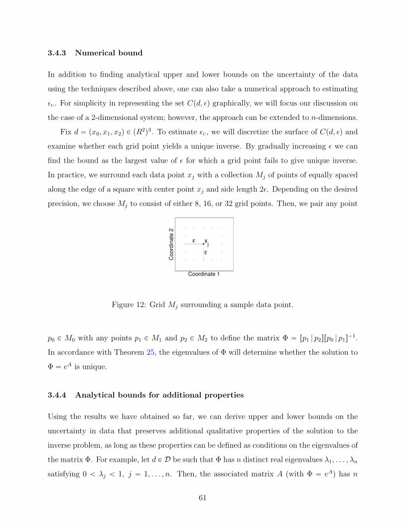
3.4.3 Numerical bound
In addition to finding analytical upper and lower bounds on the uncertainty of the data
using the techniques described above, one can also take a numerical approach to estimating
εU. For simplicity in representing the set Cpd, εq graphically, we will focus our discussion on
the case of a 2-dimensional system; however, the approach can be extended to n-dimensions.
Fix d “ px0, x1, x2q P pR2q3. To estimate εU, we will discretize the surface of Cpd, εq and
examine whether each grid point yields a unique inverse. By gradually increasing ε we can
find the bound as the largest value of ε for which a grid point fails to give unique inverse.
In practice, we surround each data point xj with a collection Mj of points of equally spaced
along the edge of a square with center point xj and side length 2ε. Depending on the desired
precision, we choose Mj to consist of either 8, 16, or 32 grid points. Then, we pair any point
Coordinate 1
Coord
inate
2
xj
ε
ε
Figure 12: Grid Mj surrounding a sample data point.
p0 P M0 with any points p1 P M1 and p2 P M2 to define the matrix Φ “ rp1 | p2srp0 | p1s´1.
In accordance with Theorem 25, the eigenvalues of Φ will determine whether the solution to
Φ “ eA is unique.
3.4.4 Analytical bounds for additional properties
Using the results we have obtained so far, we can derive upper and lower bounds on the
uncertainty in data that preserves additional qualitative properties of the solution to the
inverse problem, as long as these properties can be defined as conditions on the eigenvalues of
the matrix Φ. For example, let d P D be such that Φ has n distinct real eigenvalues λ1, . . . , λn
satisfying 0 ă λj ă 1, j “ 1, . . . , n. Then, the associated matrix A (with Φ “ eA) has n
61
distinct negative eigenvalues and hence the equilibrium is a stable node. Let εSN define the
maximal permissible uncertainty in the data d under which the equilibrium remains a stable
node. A lower bound on εSN can be obtained using the same argument as in Theorem 30,
except with the bound on maximum perturbation of eigenvalues, δU, replaced by the quantity
δSN that guarantees that the perturbed eigenvalues remain real, distinct, and between 0 and 1.
Below we present, without proofs, analytical lower bound statements analogous to Theorem
30 for the cases of a stable node and a stable system, as well as for the case in which we
require no solution to exist. We leave it to the reader to derive upper bounds using the line
of reasoning presented in Section 3.4.2.
Theorem 34. Let d P D be such that Φ has n distinct positive eigenvalues λ1, . . . , λn
satisfying 0 ă λj ă 1, j “ 1, . . . , n. Let m1 “12
miniăj|λi ´ λj|, m2 “ min1ďjďntλju,
m3 “ min1ďjďnt1´ λju and δSN “ mintm1,m2,m3u. If ε ą 0 is such that ε ď εSN “ fpδSN, dq
with f as defined in (30), then for any d P Cpd, εq, Φ has n distinct positive eigenvalues λj
with 0 ă λj ă 1, j “ 1, . . . , n, and hence the equation eA “ Φ has a unique matrix solution
A for which the origin of (2.3) is a stable node.
To guarantee stability of the equilibrium with respect to all inverse problem solutions
without demanding uniqueness of a solution, we require that d P D be such that the eigen-
values of Φ are not real negative and satisfy 0 ă |λj| ă 1, j “ 1, . . . , n. Then, the associated
matrix A (with Φ “ eA) has (possibly complex) eigenvalues with negative real part and thus
the equilibrium at the origin is stable. Let εS define the maximal permissible uncertainty in
the data d such that the equilibrium remains stable. A lower bound on εS is obtained in the
following result.
Theorem 35. Let d P D be such that the eigenvalues of Φ are not real negative and satisfy
0 ă |λj| ă 1, j “ 1, . . . , n. Let m1 “ min1ďjďnt1 ´ |λj|u, m2 “ minj|λj| for all j such that
Repλjq ą 0, m3 “ minj|Impλjq| for all j such that Repλjq ă 0 and δS “ mintm1,m2,m3u.
If ε ą 0 is such that ε ď εS “ fpδS, dq with f as defined in 30, then for any d P Cpd, εq, the
eigenvalues of Φ satisfy 0 ă |λj| ă 1, j “ 1, . . . , n and are not real negative, and hence the
equation eA “ Φ has a solution A and every such solution has all eigenvalues with negative
real part.
62
Finally, it is interesting to consider the case of nonexistence of an inverse. In particular,
given data d for which a real inverse A does not exist, i.e., data that do not represent the
trajectory of any real linear system, what is the greatest amount of uncertainty for which
nonexistence of a real solution persists, and hence a linear model should not be considered
as a possible mechanism underlying the observed uncertain data? Let d P D be such that
Φ has at least one negative real eigenvalue of odd multiplicity, which implies that there is
no real matrix A such that Φ “ eA. Let εDNE define the maximal permissible uncertainty
in the data d under which the inverse problem will be guaranteed to remain without a real
solution. A lower bound on εDNE is obtained in the following result.
Theorem 36. Let d P D be such that Φ has at least one negative real eigenvalue of odd
multiplicity. Let the collection of such eigenvalues be denoted by λ1, . . . , λk, where λk is the
closest to zero. Let m1 “ max1ďiďkpminjpj‰iq12|λj ´λi|q, m2 “ |λk| and δDNE “ mintm1,m2u.
If ε ą 0 is such that ε ď εDNE “ fpδDNE, dq with f as defined in (30), then for any d P Cpd, εq,
Φ has at least one negative eigenvalue of odd multiplicity, and hence the equation eA “ Φ
has no real solution.
3.5 EXAMPLES FOR TWO-DIMENSIONAL SYSTEMS
In the case of two-dimensional linear systems, one can represent several of the previous results
in a more explicit fashion and extend upon stability results to encompass various classifi-
cations of the equilibrium. We present these extensions here, along with several numerical
examples that can be conveniently depicted in the phase plane.
3.5.1 Regions of existence and uniqueness of the inverse
The criteria in Theorems 24 and 25 are based on the Jordan structure of Φ, which for real
2 ˆ 2 matrices can only take a few different forms, and hence can be analyzed completely.
Utilizing the relationship between the eigenvalues of a matrix and its trace and determinant,
the criteria for existence and uniqueness of the matrix logarithm of Φ can be fully charac-
63
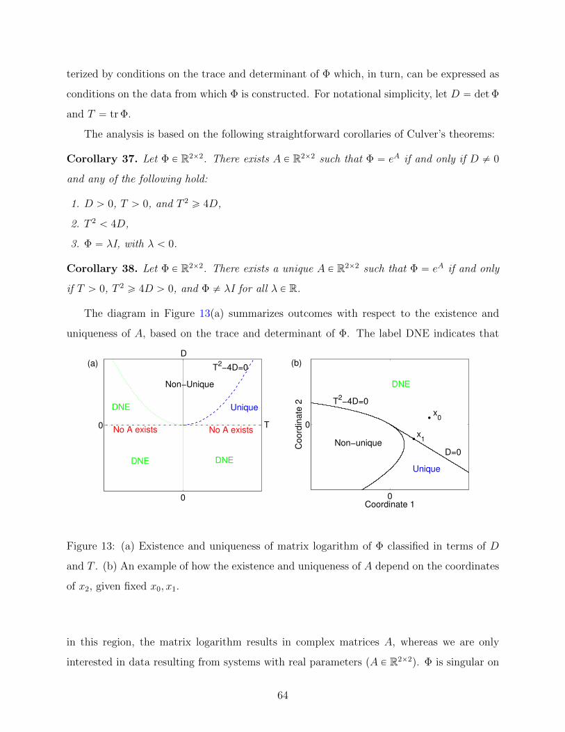
terized by conditions on the trace and determinant of Φ which, in turn, can be expressed as
conditions on the data from which Φ is constructed. For notational simplicity, let D “ det Φ
and T “ tr Φ.
The analysis is based on the following straightforward corollaries of Culver’s theorems:
Corollary 37. Let Φ P R2ˆ2. There exists A P R2ˆ2 such that Φ “ eA if and only if D ‰ 0
and any of the following hold:
1. D ą 0, T ą 0, and T 2 ě 4D,
2. T 2 ă 4D,
3. Φ “ λI, with λ ă 0.
Corollary 38. Let Φ P R2ˆ2. There exists a unique A P R2ˆ2 such that Φ “ eA if and only
if T ą 0, T 2 ě 4D ą 0, and Φ ‰ λI for all λ P R.
The diagram in Figure 13(a) summarizes outcomes with respect to the existence and
uniqueness of A, based on the trace and determinant of Φ. The label DNE indicates that
0
0
Non−Unique
DNE
DNE Unique
T2−4D=0
No A existsNo A exists
D
T
DNE
(a)
Coordinate 1
Co
ord
ina
te 2
DNE
Unique
Non−unique
x0
x1
D=0
T2−4D=0
(b)
0
0
Figure 13: (a) Existence and uniqueness of matrix logarithm of Φ classified in terms of D
and T . (b) An example of how the existence and uniqueness of A depend on the coordinates
of x2, given fixed x0, x1.
in this region, the matrix logarithm results in complex matrices A, whereas we are only
interested in data resulting from systems with real parameters (A P R2ˆ2). Φ is singular on
64
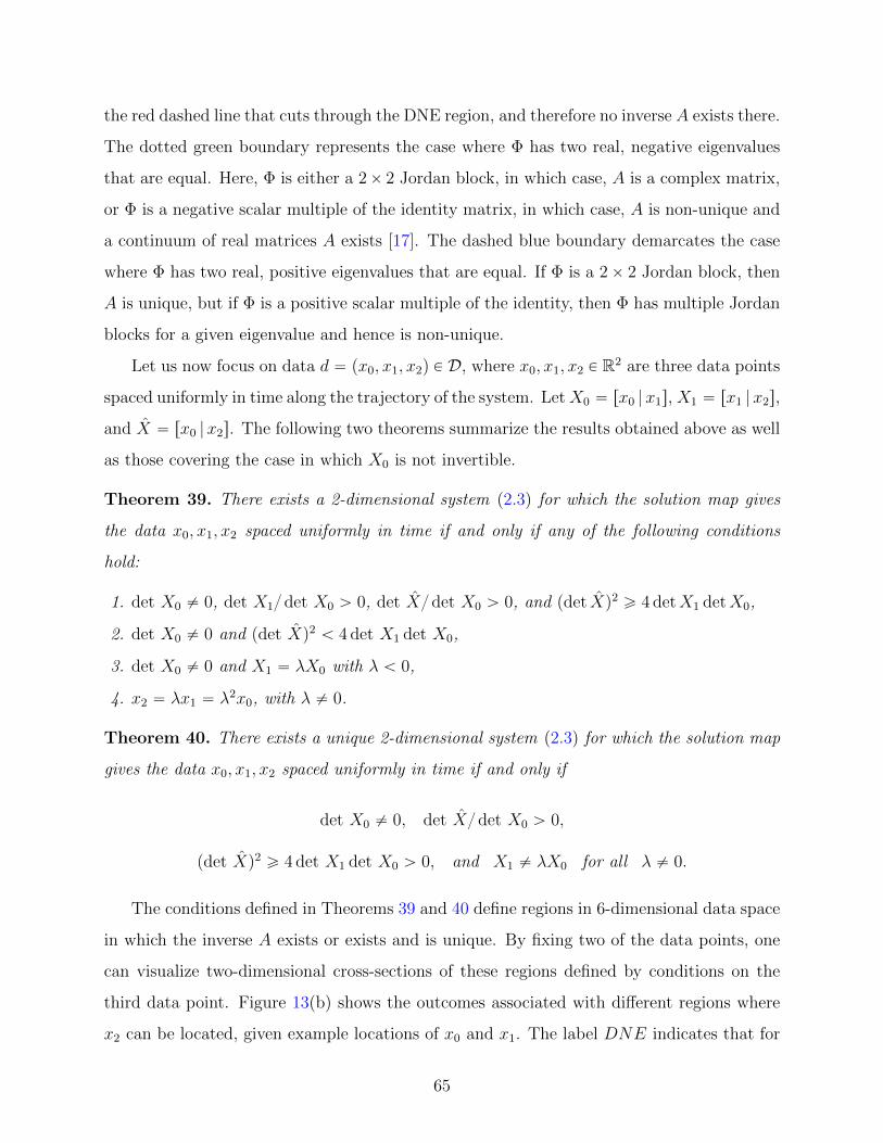
the red dashed line that cuts through the DNE region, and therefore no inverse A exists there.
The dotted green boundary represents the case where Φ has two real, negative eigenvalues
that are equal. Here, Φ is either a 2ˆ 2 Jordan block, in which case, A is a complex matrix,
or Φ is a negative scalar multiple of the identity matrix, in which case, A is non-unique and
a continuum of real matrices A exists [17]. The dashed blue boundary demarcates the case
where Φ has two real, positive eigenvalues that are equal. If Φ is a 2ˆ 2 Jordan block, then
A is unique, but if Φ is a positive scalar multiple of the identity, then Φ has multiple Jordan
blocks for a given eigenvalue and hence is non-unique.
Let us now focus on data d “ px0, x1, x2q P D, where x0, x1, x2 P R2 are three data points
spaced uniformly in time along the trajectory of the system. LetX0 “ rx0 |x1s, X1 “ rx1 |x2s,
and X “ rx0 |x2s. The following two theorems summarize the results obtained above as well
as those covering the case in which X0 is not invertible.
Theorem 39. There exists a 2-dimensional system (2.3) for which the solution map gives
the data x0, x1, x2 spaced uniformly in time if and only if any of the following conditions
hold:
1. det X0 ‰ 0, det X1 det X0 ą 0, det X det X0 ą 0, and pdet Xq2 ě 4 detX1 detX0,
2. det X0 ‰ 0 and pdet Xq2 ă 4 det X1 det X0,
3. det X0 ‰ 0 and X1 “ λX0 with λ ă 0,
4. x2 “ λx1 “ λ2x0, with λ ‰ 0.
Theorem 40. There exists a unique 2-dimensional system (2.3) for which the solution map
gives the data x0, x1, x2 spaced uniformly in time if and only if
det X0 ‰ 0, det X det X0 ą 0,
pdet Xq2 ě 4 det X1 det X0 ą 0, and X1 ‰ λX0 for all λ ‰ 0.
The conditions defined in Theorems 39 and 40 define regions in 6-dimensional data space
in which the inverse A exists or exists and is unique. By fixing two of the data points, one
can visualize two-dimensional cross-sections of these regions defined by conditions on the
third data point. Figure 13(b) shows the outcomes associated with different regions where
x2 can be located, given example locations of x0 and x1. The label DNE indicates that for
65

x2 in this region, the matrix logarithm results in complex matrices A, which means there is
no real 2-dimensional system (2.3) that gives the data x0, x1, x2.
3.5.2 Classifying the equilibrium point associated with the inverse
Theorems 39 and 40 give results on the existence and uniqueness of A based on the data.
Once we know that a real matrix A exists, additional conditions on the data may be found
that define certain important properties of the system. The classification of the equilibrium
point at the origin is easily determined by eigenvalues of A and hence can be transformed
into conditions on the data. The conditions on the classification of A in terms of properties
of Φ “ eA are given by the following statement, where again, D “ det Φ and T “ tr Φ:
Theorem 41. The equilibrium point x “ 0 of system (2.3) with matrix A P R2ˆ2 is
1. a stable node, if T ą 0, T 2 ą 4D ą 0, and 1 ą D ą T ´ 1.
2. an unstable node, if T ą 0 and T 2 ą 4D ą 4pT ´ 1q.
3. a saddle, if T ´ 1 ą D ą 0.
4. a stable spiral, if T 2 ă 4D ă 4.
5. an unstable spiral, if T 2 ă 4D and D ą 1.
6. a center, if D “ 1 and T 2 ă 4.
The region in Figure 13(a) where A is unique contains all of the systems where the
equilibrium point is a saddle or node and the region corresponding to a non-unique A contains
all of the systems where the equilibrium point is a spiral or a center (with stars on the
boundary between uniqueness and non-uniqueness). The regions described in Theorem 41
are depicted in Figure 14(a). Note that although the theorem as stated translates conditions
on A into conditions on Φ, the partitioning it provides can also be used to determine the
classification of x “ 0 for any A derived as the logarithm of a given Φ.
As in the case of Theorems 39 and 40, the conditions of Theorem 41 can be converted
to conditions on the data x0, x1, x2 P R2. Such conditions were used to construct Figure
14 (b), which describes regions in which the placement of x2, given fixed locations of x0
and x1, yields a system with a particular type of equilibrium and corresponding asymptotic
behavior. Note that, consistent with Figure 14, when data lies in the region where it uniquely
66

specifies A, the equilibrium of the resulting system is a saddle or a node, while data that
gives non-unique real A yields spirals and centers.
0
0
DNE
DNE
T2−4D=0
T
DNE
Unstable Spiral
Stable Spiral StableNode
NodeUnstable
1−T+D=0
Saddle
D=1
D(a)
D=1
1−T+D=0
T2−4D=0
D=0
Saddle
Stable
Stable
Unstable Unstable
DNE
Spiral
Spiral
Coordinate 1
Coord
inate
2 Node
Node
0
0
(b)
x0
x1
Figure 14: (a) Classification of the origin for (2.3) with A such that Φ “ eA, depicted in
terms of conditions on D “ det Φ and T “ tr Φ. Solid lines form boundaries between regions;
dashed lines do not. Note that the origin is a center for (2.3) on the solid line separating
stable and unstable spirals. (b) Conditions on the position of x2 to give dynamical systems
with specified equilibrium point types when x0 and x1 are fixed. Solid lines form boundaries
between regions; dashed lines do not.
3.5.3 Bounds on maximal permissible uncertainty
In this section we will illustrate the dependence of the maximal permissible uncertainty on
the data and the property being maintained.
Example 1. Differences between analytical bounds and numerical estimates of maximal
permissible uncertainty. Let d “ px0, x1, x2q “`
p10, 2qT , p6.065,´4.44qT , p7,´10qT˘
, which
are points that are equally spaced in time on a trajectory of the system (2.3) with
A “
»
–
´0.6724 ´0.7201
´0.8610 ´0.0244
fi
fl .
Since Φ “ eA has two distinct positive eigenvalues, A is the unique matrix that yields
the data d. For this data set, the direct numerical estimate of the maximum permissible
67
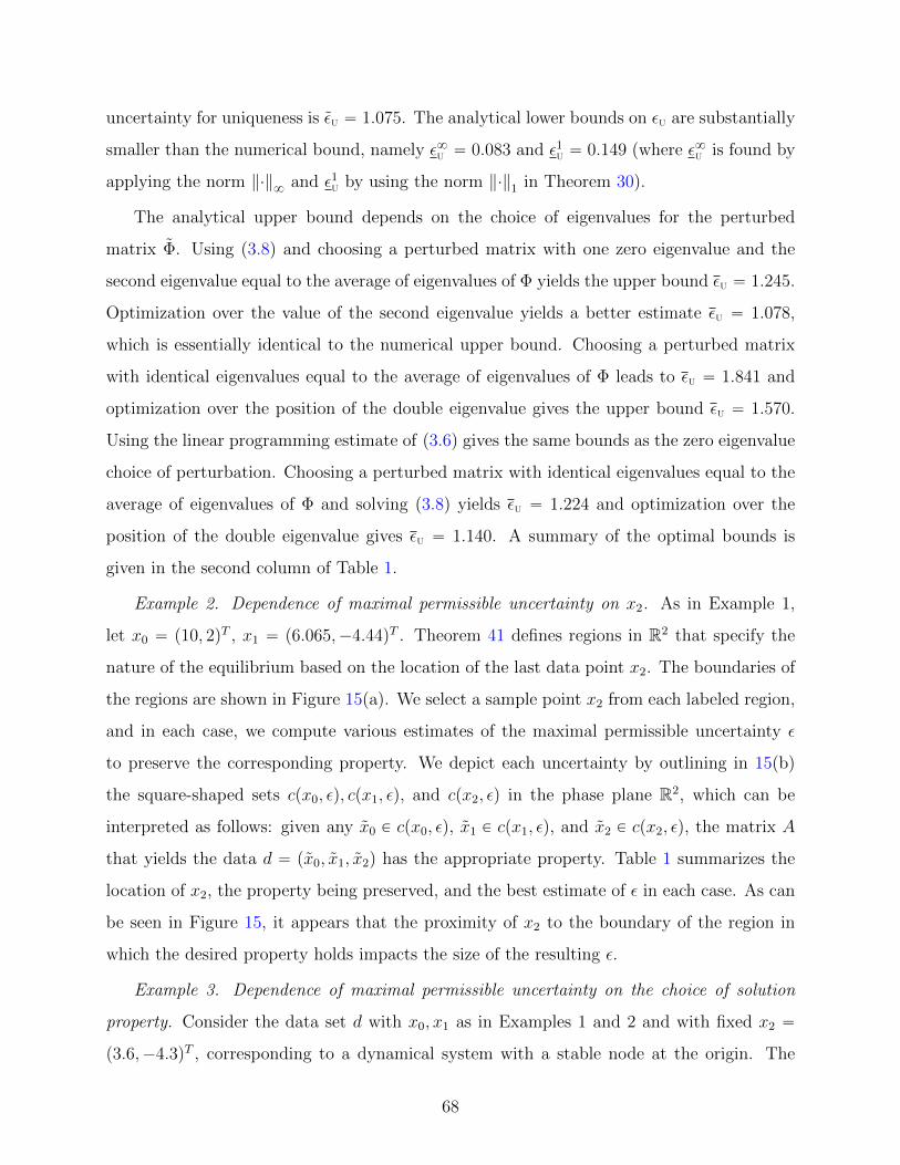
uncertainty for uniqueness is εU “ 1.075. The analytical lower bounds on εU are substantially
smaller than the numerical bound, namely ε8U “ 0.083 and ε1U “ 0.149 (where ε8U is found by
applying the norm ‖¨‖8
and ε1U by using the norm ‖¨‖1 in Theorem 30).
The analytical upper bound depends on the choice of eigenvalues for the perturbed
matrix Φ. Using (3.8) and choosing a perturbed matrix with one zero eigenvalue and the
second eigenvalue equal to the average of eigenvalues of Φ yields the upper bound εU “ 1.245.
Optimization over the value of the second eigenvalue yields a better estimate εU “ 1.078,
which is essentially identical to the numerical upper bound. Choosing a perturbed matrix
with identical eigenvalues equal to the average of eigenvalues of Φ leads to εU “ 1.841 and
optimization over the position of the double eigenvalue gives the upper bound εU “ 1.570.
Using the linear programming estimate of (3.6) gives the same bounds as the zero eigenvalue
choice of perturbation. Choosing a perturbed matrix with identical eigenvalues equal to the
average of eigenvalues of Φ and solving (3.8) yields εU “ 1.224 and optimization over the
position of the double eigenvalue gives εU “ 1.140. A summary of the optimal bounds is
given in the second column of Table 1.
Example 2. Dependence of maximal permissible uncertainty on x2. As in Example 1,
let x0 “ p10, 2qT , x1 “ p6.065,´4.44qT . Theorem 41 defines regions in R2 that specify the
nature of the equilibrium based on the location of the last data point x2. The boundaries of
the regions are shown in Figure 15(a). We select a sample point x2 from each labeled region,
and in each case, we compute various estimates of the maximal permissible uncertainty ε
to preserve the corresponding property. We depict each uncertainty by outlining in 15(b)
the square-shaped sets cpx0, εq, cpx1, εq, and cpx2, εq in the phase plane R2, which can be
interpreted as follows: given any x0 P cpx0, εq, x1 P cpx1, εq, and x2 P cpx2, εq, the matrix A
that yields the data d “ px0, x1, x2q has the appropriate property. Table 1 summarizes the
location of x2, the property being preserved, and the best estimate of ε in each case. As can
be seen in Figure 15, it appears that the proximity of x2 to the boundary of the region in
which the desired property holds impacts the size of the resulting ε.
Example 3. Dependence of maximal permissible uncertainty on the choice of solution
property. Consider the data set d with x0, x1 as in Examples 1 and 2 and with fixed x2 “
p3.6,´4.3qT , corresponding to a dynamical system with a stable node at the origin. The
68
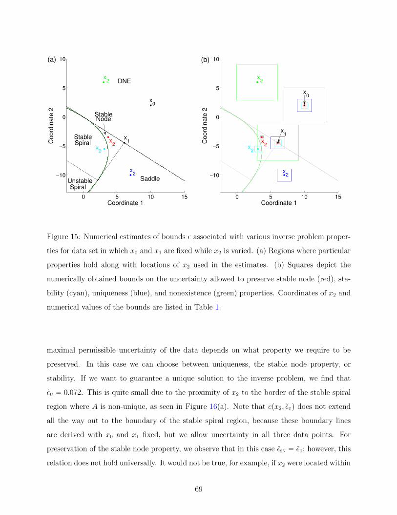
0 5 10 15
−10
0
10
5
−5
Coo
rdin
ate
2
DNE
StableSpiral
SpiralUnstable Saddle
StableNode
x0
x2
x2
x2
x2
x1
Coordinate 1
(a)
0 5 10 15
−10
0
10
5
−5
Coo
rdin
ate
2
x0
x1
x2x
2
x2
x2
Coordinate 1
(b)
Figure 15: Numerical estimates of bounds ε associated with various inverse problem proper-
ties for data set in which x0 and x1 are fixed while x2 is varied. (a) Regions where particular
properties hold along with locations of x2 used in the estimates. (b) Squares depict the
numerically obtained bounds on the uncertainty allowed to preserve stable node (red), sta-
bility (cyan), uniqueness (blue), and nonexistence (green) properties. Coordinates of x2 and
numerical values of the bounds are listed in Table 1.
maximal permissible uncertainty of the data depends on what property we require to be
preserved. In this case we can choose between uniqueness, the stable node property, or
stability. If we want to guarantee a unique solution to the inverse problem, we find that
εU “ 0.072. This is quite small due to the proximity of x2 to the border of the stable spiral
region where A is non-unique, as seen in Figure 16(a). Note that cpx2, εUq does not extend
all the way out to the boundary of the stable spiral region, because these boundary lines
are derived with x0 and x1 fixed, but we allow uncertainty in all three data points. For
preservation of the stable node property, we observe that in this case εSN “ εU; however, this
relation does not hold universally. It would not be true, for example, if x2 were located within
69

Table 1: Best Estimates of εX, X P t SN, U, S, DNE u, for Example 2
Property (X) Stable Node (SN) Unique (U) Stable (S) Nonexistence (DNE)
x2 p3.68,´3.46q p7,´10q p3.1,´5.5q p3, 6q
εX Numerical estimate 0.216 1.075 0.519 3.055
εX by Theorem 30 0.059 0.149 0.207 0.609
εX by (3.6) 0.217˚ 1.078: 0.519; 3.059#
εX by (3.8) 0.251˚ 1.078: 0.665; 3.683:
˚λ1 “ λ2, :λ1 “ 0, ;λ2 “ 1, #λ2 Ñ8
the stable node region but closer to the saddle region where A is unique (e.g., see Example
4 below). If we want to ensure that the data lie on a trajectory that converges to the origin
(i.e., preserve the stability of the system), we find that the maximal permissible uncertainty
is εS “ 0.647, which is significantly larger than εU. Thus we can guarantee stability for
larger uncertainty in the data than what is needed to preserve the uniqueness of solutions.
Figure 16(a) depicts the data in the phase plane and the numerically computed maximal
permissible uncertainties for the uniqueness, stable node, and stability properties. Within
the set Cpd, εSq, any choice of data will lie on a stable trajectory, however, the uniqueness
of the inverse problem may not be preserved. In 16(b) we illustrate two different data sets
contained in Cpd, εSq; one data set on a stable node trajectory (red), corresponding to a
unique A, and a second data set belonging to a stable spiral trajectory (blue), where A is
not unique.
Example 4. Dependence of maximal permissible uncertainty on the choice of solution
property. Consider the data set d with x0, x1 as in Examples 1-3 and with x2 “ p5,´5.6qT ,
which corresponds to a stable node equilibrium. Again, the maximal permissible uncertainty
of the data depends on what property we require to be preserved. Here we find that εSN “
70
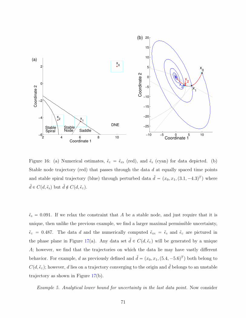
2 4 6 8 10−6
−4
−2
0
2
Coord
inate
2
SaddleStableStable
Spiral Node
DNE
x1
x2
x0
Coordinate 1
(a)
−10 −5 0 5 10
−25
−20
−15
−10
−5
0
5
10
15
20
Co
ord
ina
te 2
x2
x2
x1
x0
Coordinate 1
(b)
Figure 16: (a) Numerical estimates, εU “ εSN (red), and εS (cyan) for data depicted. (b)
Stable node trajectory (red) that passes through the data d at equally spaced time points
and stable spiral trajectory (blue) through perturbed data d “ px0, x1, p3.1,´4.3qT q where
d P Cpd, εSq but d R Cpd, εUq.
εS “ 0.091. If we relax the constraint that A be a stable node, and just require that it is
unique, then unlike the previous example, we find a larger maximal permissible uncertainty,
εU “ 0.487. The data d and the numerically computed εSN “ εS and εU are pictured in
the phase plane in Figure 17(a). Any data set d P Cpd, εUq will be generated by a unique
A; however, we find that the trajectories on which the data lie may have vastly different
behavior. For example, d as previously defined and d “ px0, x1, p5.4,´5.6qT q both belong to
Cpd, εUq; however, d lies on a trajectory converging to the origin and d belongs to an unstable
trajectory as shown in Figure 17(b).
Example 5. Analytical lower bound for uncertainty in the last data point. Now consider
71

0 2 4 6 8 10−10
−8
−6
−4
−2
0
2
Co
ord
ina
te 2
Saddle
StableStableSpiral
Node
DNE
x1
x2
x0
Coordinate 1
(a)
0 2 4 6 8 10−10
−8
−6
−4
−2
0
2x
0
x1
x2
x2
Coordinate 1
Co
ord
ina
te 2
(b)
Figure 17: (a) Numerical estimates εS,“ εSN (red) and εU (blue) for the data depicted. (b)
Stable trajectory (red) through the data d and unstable trajectory (blue) through perturbed
data d P Cpd, εUq.
the case where the data points x0 and x1 are fixed at the same values as in Examples 1-4 and
we seek to find the maximum uncertainty εU allowed in the last data point x2 such that for
any x2 P cpx2, εUq, there is a unique A that gives the data d “ px0, x1, x2q at equally spaced
time points. Let x2 “ p3.679,´3.459qT . We find the numerical estimate εU “ 0.423 and the
analytical estimates ε1U “ 0.07 and ε8U “ 0.187 (using Theorem 33). In this case, the difference
between the numerical and analytical lower bounds is much improved from Example 1, and
the lower bound, which is the only easily computable bound in higher dimensions, becomes
quite useful. Pictured in Figure 18 are the boundaries of the sets cpx2, εUq (red) and cpx2, ε8U q
(green) along with the functions dividing the plane into regions where x2 may lie such that
the parameter A that produces that data is unique or non-unique. As expected, we observe
that cpx2, εUq and cpx2, ε8U q are contained in the region corresponding to a unique A.
72
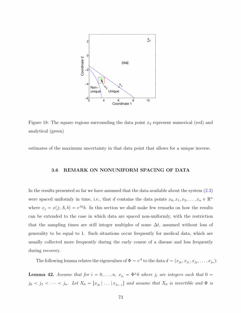
2 4 6 8 10−6
−4
−2
0
2
Coordinate 1
Co
ord
ina
te 2
x1
x0
x2
DNE
UniqueNon− unique
Figure 18: The square regions surrounding the data point x2 represent numerical (red) and
analytical (green)
estimates of the maximum uncertainty in that data point that allows for a unique inverse.
3.6 REMARK ON NONUNIFORM SPACING OF DATA
In the results presented so far we have assumed that the data available about the system (2.3)
were spaced uniformly in time, i.e., that d contains the data points x0, x1, x2, . . . , xn P Rn
where xj “ xpj;A, bq “ eAjb. In this section we shall make few remarks on how the results
can be extended to the case in which data are spaced non-uniformly, with the restriction
that the sampling times are still integer multiples of some ∆t, assumed without loss of
generality to be equal to 1. Such situations occur frequently for medical data, which are
usually collected more frequently during the early course of a disease and less frequently
during recovery.
The following lemma relates the eigenvalues of Φ “ eA to the data d “ pxj0 , xj1 , xj2 , . . . , xjnq:
Lemma 42. Assume that for i “ 0, . . . , n, xji “ Φjib where ji are integers such that 0 “
j0 ă j1 ă ¨ ¨ ¨ ă jn. Let X0 “ rxj0 | . . . |xjn´1s and assume that X0 is invertible and Φ is
73
nonsingular. Let y “ X´10 xjn be a vector with entries y1, y2, ..., yn. Then λ is an eigenvalue
of Φ only if λ is a root of the polynomial
λjn ´ ynλjn´1 ´ ¨ ¨ ¨ ´ y2λ
j1 ´ y1 “ 0. (3.9)
Proof. Since y “ X´10 xjn , it follows that xjn “ X0y, i.e.,
Φjnb “n´1ÿ
i“0
yi`1Φjib. (3.10)
The assumption that X0 is invertible is equivalent to the statement that the vectors txjiun´1i“0
are not confined to a proper subspace of Rn and hence, if xji “ Φjib “ eAjib, b is not
confined to a proper Φ-invariant subspace of Rn. Thus b, when decomposed in the basis of
ordinary and generalized eigenvectors of Φ, has a nonzero component along the ordinary or
generalized eigenvector for every eigenvalue of Φ. Let v be the eigenvector corresponding to
the eigenvalue λ of Φ. If b has a nonzero component along v, then (3.10) implies that
λjnv “n´1ÿ
i“0
yi`1λjiv,
which proves the statement. If the component of b along v is zero but b has a nonzero
component along u such that pA´λIqk´1u ‰ 0 and pA´λIqku “ 0, then (3.10) implies that
λjn`ku “n´1ÿ
i“0
yi`1λji`ku,
which for nonzero λ reduces to the previous case.
74

Lemma 42 is employed in solving the inverse problem as follows: First, the vector y is
computed from the data d “ pxj0 , xj1 , xj2 , . . . , xjnq. Second, all roots of the polynomial (3.9)
are found using numerical techniques. Third, a combination of n distinct roots is chosen from
the collection of roots. Fourth, the companion matrix Φ of Φ is formed from the chosen roots
and a set of vectors zji , i “ 0, 1, ..., n´1 is computed by taking z0 “ e1 and zji`1“ Φji`1´jizji .
Finally, the matrix Φ is found as Φ “ P´1ΦP where P is the (unique) n ˆ n matrix such
that Pxji “ zji for i “ 0, 1, ..., n´ 1.
The procedure outlined above can find any matrix Φ that is robust, in the sense of
Corollaries (27)-(29). The condition that X0 be invertible (i.e., b not be confined to a proper
Φ-invariant subspace) is essential for identifiability of Φ, as we have already observed in
Chapter 2 for the special case of ji “ i. If the indices ji differ by more than 1 then the
polynomial (3.9) has more roots than the matrix Φ has eigenvalues. Arbitrary combinations
of such roots will lead to different alternative matrices Φ and hence to non-uniqueness of
solutions of the inverse problem. By an appropriate choice of the roots that make up the
eigenvalues of Φ, one may be able to control the properties of the matrix Φ and, in turn,
the existence, uniqueness, and stability properties of the parameter matrix A of the system
(2.3).
3.7 DISCUSSION
We have analyzed the inverse problem for linear dynamical systems, i.e., the problem of find-
ing the value of the parameter matrix for which a linear system generates a given discrete
data set consisting of points equally spaced in time on a single trajectory. Our results estab-
lish regions in data space that give solutions with particular properties, such as uniqueness
or stability, and give bounds on the maximal allowable uncertainty in the data set that can
be tolerated while maintaining these characteristics.
Three types of bounds on uncertainties are presented: analytical lower bounds, below
which properties are guaranteed to hold for all perturbations of data; analytical upper
bounds, which provide proven perturbations of data for which properties are guaranteed
75

to be lost; and numerical bounds, derived from direct sampling of data points. Our results
indicate that the upper bounds, when optimized over all potential eigenvalues, provide ex-
cellent agreement with the numerical estimates The numerical methods are hypothetically
applicable to systems of arbitrary size; however, the combinatorial problem of pairing to-
gether all possible data points along grid points can pose a challenge as the dimension of
the system increases. Similarly, the computation of the analytical upper bound (via (3.6)
or (3.8)) requires optimization that becomes computationally expensive for larger systems.
Although the analytical lower bound significantly underestimates the maximal permissible
uncertainty, it provides a bound that is immediately accessible for systems of higher dimen-
sion, without increased computation. Since we focused on the derivation of these bounds,
the question of how these bounds scale with system size remains open for future investiga-
tion. Furthermore, in this work, we have considered only random perturbations of the data
matrix Φ. Due to the special construction of the matrix Φ, it may be possible to improve
the analytical lower bound by considering structured matrix perturbations. Many results
have been established concerning the bounds on eigenvalues for structured perturbations of
matrices [42, 39] that may prove useful in this effort.
A variety of earlier works considered identification of linear systems or parameter matrices
from discrete data. Allen and Pruess proposed a method for approximating A in system
(2.3) from a discrete collection of data points [2]. Their approach begins by defining an
approximating function for the data (e.g., a cubic spline approximation), and they use equally
spaced points along this curve to compute a matrix A that approximates the true parameter
matrix A. A key distinction between their work and the initial analysis presented here is
that they use points on an approximation of the trajectory, while we assume that the data
represent exact points on the actual trajectory; their results also do not treat uncertainty in
data.
In other past work, Singer and Spilerman investigated the problem of identifying the
matrix Q in the Markov model P 1 “ QP where P and Q are n ˆ n matrices [73]. They
derive conditions for P “ eQ to have a unique solution. Their results are consistent with the
findings of Culver, but with additional constraints to account for the requirement that the
model is a continuous time Markov structure. They additionally comment on the case of
76
identifying Q from noisy observations and suggest exploring in a neighborhood of P in order
to detect non-uniqueness of the matrix logarithm through observations on the eigenvalues of
the matrices in this neighborhood.
It is of interest to note that much work has been done in determining the maximal
allowable uncertainty in the parameter matrix A such that the solution to (2.3) remains
stable [39]. This well known bound is called the stability radius. In our investigation of the
inverse problem, εS has an analogous meaning, but we quantify the uncertainty in the data
space rather than in parameter space.
Our results also include bounds on regions of data space where the inverse problem
cannot be solved. The utility of such results is that they can provide an approach for model
rejection. That is, suppose we have a data set d acquired from measurements of some physical
phenomenon that we believe can be modeled with a linear system of differential equations.
Perhaps it is known that the measurement error for any data point xi is approximately given
by ε. If we find that there is no real matrix A that yields the collected data d and further
find that εDNE ą ε, then we can conclude with certainty that the data cannot come from a
system that can be modeled with a linear system of differential equations, and thus we can
reject the linear model.
Our work is also related to the important problem of determining identifiability in pa-
rameter estimation. The connection to identifiability is apparent if we consider the set in
parameter space defined by F´1pCpd, εUqq. On this set we have that F´1pd1q ‰ F´1pd2q im-
plies d1 ‰ d2 P Cpd, εUq, which is to say that two distinct parameter sets must yield distinct
data. So, F´1pCpd, εUqq defines a set in parameter space on which the model is identifiable.
In the next chapter, important aspects of parameter estimation from a collection of single
trajectory data will be investigated. In this practical setting, we will study improvements to
Monte Carlo techniques used in Bayesian parameter estimation.
77

4.0 THE JACOBIAN PRIOR IMPROVES PARAMETER ESTIMATION
WITH THE METROPOLIS-HASTINGS ALGORITHM
4.1 INTRODUCTION
Once a model structure is fixed and experimental data is collected, the problem of determin-
ing the unknown model parameters must be confronted. In a Bayesian inference approach to
parameter estimation, a posterior distribution of parameters which describes the probability
of a parameter governing the system given the available data, is sought. Markov chain Monte
Carlo methods provide a means to sample this distribution. One widely used computational
method which employs this approach is the Metropolis-Hastings algorithm. Implementation
of this algorithm for Bayesian parameter estimation requires the prescription of a prior den-
sity of parameters, which reflects any previously known information about the parameters.
The choice of a prior may greatly impact the posterior obtained from the algorithm and has
been a topic of debate among practitioners [10, 32, 68, 74]. In this chapter, we introduce
a new informative prior which does not rely on previous information about the parameters
alone, but exploits knowledge of the fixed model structure.
The presentation of the chapter is as follows: In the first section, the notation for the
models of interest and other important constructs that will be used in this chapter are
defined. In Section 4.2.2, background on Bayesian inference for parameter estimation is dis-
cussed, followed by an introduction to the Metropolis-Hastings algorithm. In Section 4.3,
we present the theoretical derivation of the Jacobian prior. We then work to systemati-
cally analyze the accuracy of the posteriors obtained using this newly proposed prior in the
Metropolis-Hastings algorithm. In Section 4.4.1, the known solution to systems of linear dif-
ferential equations is exploited and the analysis of Chapter 3 is utilized in order to define the
78

parameter density explicitly. This provides the exact solution to the parameter estimation
problem as a means for comparison to the posteriors obtained from the Metropolis-Hastings
algorithm. Two different systematic approaches for analyzing the accuracy of the posteriors
are presented. Through a series of several examples, we find that using the Jacobian prior
results in posteriors that closely match the parameter density and frequently yields more ac-
curate results than with other commonly used priors. In Section 4.4.2, we conduct a similar
analysis of comparison between the parameter density and the computed posteriors, instead
for a nonlinear system of differential equations. The chapter concludes with a discussion in
Section 4.5.
4.2 PRELIMINARIES
4.2.1 Model and notation
The model of interest is formulated as an initial-value problem for a system of ordinary
differential equations,
9xptq “ gpxptq,Λq
xp0q “ b.(4.1)
In equation (4.1), xptq P Rn is the state of the system at time t, Λ is a vector of parameters,
and b P Rn is the initial condition. The initial condition or a subset of its components may
be unknown and thus considered as parameters. Then, the model parameters, denoted by
a P Rp, is a vector comprised of Λ and any parameter elements of b. For notational simplicity,
the parameter space will be called A.
We shall assume that model (4.1) is well posed and the solution (or trajectory), denoted
by xpt; Λ, bq, is unique for all Λ and b. We assume that data for all of the state variables is
available and denote by Y , the data space consisting of a set of m-tuples y “ px1, x2, . . . , xmq
of points xj P Rn, representing observations of the system at times t1, t2, . . . tm. Observations
of the trajectory xpt; Λ, bq at times t1, t2, . . . , tm yields an element of Y , namely an m-tuple
of points xj “ xptj; Λ, bq P Rn, j “ 1, . . . ,m. In this work, we will require p “ nm. The
79
term solution map will refer to the map F : A Ñ Y from parameter space to data space,
defined as F paq “ px1, x2, . . . , xmq “ y for a choice of txju sampled from xpt; Λ, bq.
Y will denote the available data for the system which will be used in the inverse problem
of determining the model parameters. In the case of a collection of single trajectory data,
Y “ ty1, y2, . . . yNu with yj P Y may represent N repeated observations of the system or
N subjects from which experimental measurements are drawn. Alternatively, Y may be
provided as a set of mean values tx1, . . . , xmu and standard deviations tσ1, . . . σmu, or in an
idealized setting, Y may be a density on the data space, denoted by Y “ ηpyq.
A number of approaches have been developed for parameter estimation of differential
equation models. In traditional parameter fitting techniques, a cost function, which quanti-
fies the agreement between the measured data and the model predicted values of the output,
is constructed. For example, if the data Y are assumed to be normally distributed random
variables with mean values tx1, . . . , xmu and standard deviations tσ1, . . . σmu, then the cost
function may be represented as a sum of squared residuals between the measured data and
the model trajectory:
Epa, Y q “ÿ
i
ÿ
j
pxjpti, aq ´ xi,jq2
2σ2i,j
.
The solution to the parameter estimation problem is the parameter a˚ which minimizes
the cost function. The vector a˚ is called the maximum likelihood estimate of the parame-
ters. One commonly employed algorithm for minimizing the cost function is the Levenberg-
Marquardt scheme [51].
Another parameter estimation approach is the multiple shooting algorithm. In this
method, the initial value problem is converted to multiple boundary value problems that
are solved for segments of the full trajectory [12, 85]. This method is particularly useful for
stiff or chaotic systems. Another popular approach is the Kalman filter technique. Here,
a recursive algorithm updates the parameters by minimizing the discrepancy between the
model predicted output and the data as successive data points are incorporated [49]. There
are several variations and extensions of the Kalman filter for nonlinear systems [87].
Each of the methods discussed above produces a single parameter vector as the solution
to the inverse problem. Alternatively, probabilistic approaches, such as Bayesian inference,
output a distribution of parameters rather than a unique set of parameters. Such an approach
80

may be especially relevant in biological modeling. In this setting, the model parameters may
represent biological quantities that naturally vary from individual to individual. In this
case, the parameter distribution represents parameter variability between individuals in a
population. Together, the parameter distribution and the system of differential equations
form a collection of models often referred to as an ensemble. A discussion of ensemble
modeling for biological systems may be found in [77]. The objective is then to find the best
approximation to the density ρpaq that describes the parameter distribution.
4.2.2 Bayesian inference for parameter estimation
In a Bayesian inference approach to parameter estimation, one aims to approximate the
parameter density ρpaq with a posterior density ρpa|Y q, which makes use of the available
data. Given a fixed model structure and the data Y , the posterior density of the parameters
ρpa|Y q quantifies the probability that the system is governed by the parameters a given
the data Y . Fundamental theory of Bayesian inference and its applications to parameter
estimation are discussed in [33, 74]. Bayes’ Theorem provides a crucial relation between the
unknown posterior density and a known likelihood function LpY |aq and prior density πpaq.
Bayes’ Theorem: ρpa|Y q “LpY |aqπpaq
ş
LpY |aqπpaqda. (4.2)
The likelihood function LpY |aq quantifies the deviation of the model with parameters a from
the available data, Y . The function LpY |aq (with a as the dependent variable and Y fixed)
is defined by the statistical model of the data (where the error comes from and what is the
distribution of the error). For example, suppose the data observations xi are assumed to be
normally distributed random variables, and Y is provided as a set of mean observation values
tx1, . . . , xmu and standard deviations tσ1, . . . σmu. If the errors in the data measurements
are independent and identically distributed, then the likelihood function can be defined as
LpY |aq “ź
i
Lipxi|aq
where,
Lipxi|aq “ź
j
1
σi,j?
2πe´pxjpti;aq´xi,jq
2
2σi,j2
.
81

Alternatively, in an idealized setting, the data Y could be given as a density function ηpyq.
The solution to model (4.1) is unique and due to the absence of error in the forward model
solution, it holds that the likelihood can be defined as Lpη|aq “ ηpF paqq ([79], page 35).
Several other likelihood functions may be defined based upon properties of the data available,
for example by taking into account covariances in the data. Thoughtful selection of the
likelihood function is important because the data informs the posterior only through the
likelihood.
The prior density πpaq reflects any information that is known about the parameters before
data is considered. This information may include bounds on the values of the parameters
which are obtained from literature (e.g. biological experiments) or from qualitative analysis
of the system (e.g. analysis of existence and stability of equilibria).
A noninformative prior (also commonly referred to as an objective or flat prior) may be
used when no information about the parameter values is known. This prior is flat relative to
the likelihood, thus minimizing its impact on the posterior distribution. A uniform density
posed on the support of the parameters is a commonly used noninformative prior [74]; for
example πpaq “ χr0,8q
paq is a uniform prior density for a positive parameter (this is an
improper prior because its integral is infinite). Jeffreys prior is an objective prior based
on the Fisher information matrix [45]. This prior does not vary much over the region in
which the likelihood is significant and does not take on large values outside that range, thus
satisfying the local uniformity property [29]. It also has the property of scale invariance,
meaning that it is invariant under reparameterization by injective transformations. An
informative prior can be used when characteristics of the parameters are known a priori.
Unlike noninformative priors, this prior is not dominated by the likelihood.
The choice of a prior is a topic of debate among practitioners of Bayesian inference
[10, 32, 68, 74]. The possible dangers of employing an informative prior are illustrated by
Smith in [74]. He shows that a poorly chosen informative prior can degrade the accuracy of
the posterior far more than an objective prior and recommends that unless good previous
information is known, an objective prior should be used. This chapter represents a contri-
bution to the investigation of prior density selection by introducing a new informative prior
which is specifically relevant for Bayesian inference in the setting of parameter estimation.
82

4.2.3 Metropolis-Hastings algorithm
In practice, a sample of the posterior density ρpa|Y q can be obtained using Markov chain
Monte Carlo (MCMC) techniques. In the setting of Bayesian inference, the Metropolis-
Hastings algorithm constructs a Markov chain a1, a2, . . . , aM with the posterior density as
its limiting distribution [35, 61]. This approach to parameter estimation is widely used in
practice and the Metropolis-Hastings algorithm has been referred to as one of the top ten
algorithms of the twentieth century [74]. Accessible introductions to the algorithm can be
found, for example, in [74, 81]. In each iteration of the algorithm, ρpa|Y q will be computed
using Theorem 4.2 with the normalization constant omitted, as will be discussed below.
Given the model (4.1) and the available data Y , the algorithm is formulated as follows:
1. Choose an initial parameter value a1 satisfying ρpa1|Y q ą 0.
2. For k “ 1, . . .M ,
(i) Propose a new parameter value a from a proposal (jumping) distribution qpa|akq.
(ii) Using a, solve the ODE system (4.1) and compute ρpa|Y q “ LpY |aqπpaq.
(iii) Set
ak`1“
$
&
%
a , with probability min!
1, ρpa|Y qqpak|aqρpak|Y qqpa|akq
)
pa acceptedq
ak, otherwise pa rejectedq.
The proposal distribution q for selecting a is based only on the previous parameter ak, thus
creating a Markov process. In the case that q is symmetric, it follows that qpak|aq “ qpa|akq
and the probability of accepting a as ak`1 in step 2(iii) simplifies to
min
"
1,ρpa|Y q
ρpak|Y q
*
.
The variance of the proposal distribution greatly influences the exploration in parameter
space. Large variance may cause most of the proposals to be rejected due to small likelihoods,
thus the resulting chain remains stationary for many iterations. If the variance is chosen to
be too small, the acceptance ratio will be high, but the exploration of the parameter space
will be slow. Additionally, estimating an anisotropic posterior using an isotropic proposal
distribution will decrease the efficiency of the exploration of the space [74]. It is recommended
83

that the variance of the proposal distribution should be chosen so that on average, 25% of
the proposals are accepted [77].
Step 2(ii) of the algorithm provides the connection to Bayes’ Theorem. The likelihood
function LpY |aq and the prior πpaq must be prescribed, and the resulting posterior may
be highly influenced by this choice, as will be revealed in later examples. Note that in
the computation of ρpa|Y q “ LpY |aqπpaq, the normalization constant is omitted. It is
unnecessary to include this constant because in the ratio of posteriors used for the acceptance
criterion, it is eliminated.
The acceptance criteria in step 2(iii) provides a means through which the chain can escape
a local maximum in ρpa|Y q. In the case of a symmetric proposal density, if ρpa|Y q ě ρpak|Y q
then a is accepted with probability 1, otherwise when ρpa|Y q ă ρpak|Y q the probability of
accepting a decreases as ρpa|Y q decreases.
The sequence a1, a2, . . . , aM produced by the algorithm is a Markov chain that, in the
limit of M Ñ 8, has the posterior density as its stationary distribution. How long the
chains must be run to converge and sufficiently sample from the posterior is a challenging
question, and analytic convergence and stopping criteria are lacking [74]. A burn in period,
where the first j elements of the chain are thrown out, is often employed because in the
initial part of the algorithm, the proposals are not sampled from the stationary distribution.
Several techniques have been introduced to improve exploration of the space and speed
up convergence. For example, parallel tempering makes use of several Markov chains run
simultaneously with different variances in the proposal distribution [20]. Swapping between
the chains allows for refined sampling in regions near extrema and improved mixing, so
that chains do not become stuck in local extrema. This approach can be computationally
expensive. A less sophisticated, but useful means of improving mixing is to introduce a
random proposal a selected from a uniform distribution on the parameter support every X
iterations of the algorithm (e.g. X “ 10). This approach allows the chain to escape local
extrema and increases the convergence rate of the chain.
84

4.3 THEORETICAL DERIVATION OF THE JACOBIAN PRIOR
In this section, we assume that the data is given as the distribution ηpyq and derive a prior
density that will facilitate exact solution of the inverse problem when Bayesian inference is
employed. We will propose the use of this prior in the Metropolis-Hastings algorithm and
examples will be presented in following sections.
As defined in section (4.2.1), A is the parameter space, Y is the data space of observations,
and F : AÑ Y represents the forward solution map from model parameters to data. Define
ρpaq to be the parameter density, representing the distribution of parameters for the model.
Let ηpyq be a density on the data space, such that for any measurable Ω Ď A, we have that
F pΩq Ď Y andż
F pΩq
ηpyqdy “
ż
Ω
ρpaqda. (4.3)
If Ω is any subset of A (of positive measure) on which F is injective, then by the well known
change of variables formula (Theorem 2.47 [26]),
ż
F pΩq
ηpyqdy “
ż
Ω
ηpF paqq| detDaF paq|da “
ż
Ω
ηpF paqqJpaqda where Jpaq “ | detDaF paq|.
Thus, from equation (4.3), for any Ω Ď A on which F is injective,
ż
Ω
ρpaqda “
ż
Ω
ηpF paqqJpaqda,
and therefore,
ρpaq “ ηpF paqqJpaq. (4.4)
In the Bayesian inference approach, the posterior density is determined by making use
of the available data. The density ηpyq on the data provides an ideal setting, in which full
information about the data is known. The Bayes relation (4.2) with Y “ ηpyq, gives that
the posterior density, ρpa|ηq, is proportional to the likelihood times the prior. That is,
ρpa|ηq “ kLpη|aqπpaq,
where πpaq is the prior density on the parameters, Lpη|aq is the likelihood of the data given
an element a of the parameter space, and k is a normalization constant. In the absence of
85
error in the forward model solution, it holds that Lpη|aq “ ηpF paqq, ([79], page 35) and thus,
ρpa|ηq “ kηpF paqqπpaq. (4.5)
In order for the posterior ρpa|ηq to be equal to the parameter density ρpaq, it follows from
equations (4.4) and (4.5), that the prior should be chosen as
πpaq “Jpaq
k. (4.6)
We will refer to Jpaq as the Jacobian prior, following the conventional terminology in
which DaF paq is called the Jacobian. We note that the term Jacobian prior has appeared
previously [78], in the computation of a marginal with a change of variables, however the
context is different and it does not appear to be a commonly used term. This informative
prior is not simply based on previous knowledge of the parameters, but rather, on prior
knowledge of the model structure and the connection between model parameters and the
data (i.e. the solution map F ). This derivation relies heavily on the injectivity of F , which
is guaranteed when the model (4.1) is identifiable. In the following section, we will use the
analysis of Chapter 3, where explicit sets on which F´1 exists were established, in order to
systematically study the accuracy of the posterior densities obtained by using the Jacobian
prior in the Metropolis-Hastings algorithm.
4.4 SYSTEMATIC ANALYSIS OF THE INFLUENCE OF THE PRIOR
In this section, a systematic approach will be used to demonstrate the superiority of the
performance of the Jacobian prior in the Metropolis-Hastings algorithm with that of other
commonly used priors. In particular, the parameter density ρpaq will be constructed for
comparison with the posterior densities ρpa|ηq obtained from implementing the Metropolis-
Hastings algorithm with various priors.
Model (4.1) is selected to be locally identifiable, thus guaranteeing the injectivity of
F . We will assume there is full knowledge of the data, given by the density ηpyq. The
injectivity of F directly relates ηpyq to a parameter density ρpaq by equation (4.3). With
86

Figure 19: Visual summary of the method used to compare the parameter density ρpaq to the
posteriors ρpa|ηq obtained using various priors πpaq in the Metropolis-Hastings algorithm.
this construction, ρpaq is the parameter density of the system under consideration (to be
determined from the data). Using ηpyq for the data, the Metropolis-Hastings algorithm is
implemented with various priors πpaq to produce the corresponding estimates of the posterior
density ρpa|ηq. The posteriors obtained using the various priors can then be compared to the
parameter density ρpaq and to each other. Figure 19 provides a schematic diagram describing
this systematic approach.
In the Bayes relation (4.2), the data directly informs the posterior only through the
likelihood. Using ηpyq as the data we have seen that Lpη|aq “ ηpF paqq (due to the absence
of error in the forward model solution). This eliminates uncertainty in the estimation of
ρpa|ηq due to the data and isolates the prior as the primary source of error, thus truly
revealing the effect of the prior.
In the following section, we will use the approach introduced above to study the effective-
ness of the Jacobian prior in obtaining accurate estimates of the posterior density with the
Metropolis-Hastings algorithm. In the case of linear systems of ordinary differential equa-
tions, we will use the analysis of Chapter 3 in order to explicitly define the density ηpyq. In
other circumstances, ηpyq cannot be defined exactly and must be estimated. Two different
approaches will be presented in order to address both of these situations.
87

4.4.1 Linear systems
Consider the linear system of differential equations defined as
9xptq “ Λxptq
xp0q “ b(4.7)
where xptq P Rn is the state of the system at time t, Λ P Rnˆn is a matrix of parameters,
and b P Rn is the initial condition, which is now taken as a fixed known value rather
than a free parameter. Since the initial condition is independent of the parameters, the
model parameters are the entires of the matrix Λ written as a vector a P Rn2and the
parameter space is A “ Rn2. As in Chapter 3, the data will be observed at n equally
spaced time intervals (without loss of generality ∆t “ 1) tj “ j, j “ 1, . . . , n, yielding
y “ px1, . . . , xnq P Y with xj P Rn. Using n time points ensures that DaF paq is a square
matrix.
Defining model (4.1) to be a linear system of differential equations provides several
advantages in using our systematic approach to study the Jacobian prior. In Chapter 3,
the existence of sets in the data space Y on which F´1 exists for the linear dynamical
system (4.7) was established. Due to the injectivity of F , the Jacobian, Jpaq, can be used
as the prior in the Metropolis-Hastings algorithm. The invertibility of F will be exploited to
construct a direct sample of the parameter density ρpaq, which will be used to compare with
the posteriors obtained by employing various priors in the Metropolis-Hastings algorithm.
4.4.1.1 Comparison of priors: Approach 1 Implementation of the systematic ap-
proach described by Figure 19, in practice, requires sampling of the densities and additional
modifications from the abstract setting. The following description details our first method
for applying this approach and Figure 20 provides a corresponding schematic diagram.
1. Fix y P Y such that F´1pyq “ a is unique (i.e. y such that the associated Φ “
rx1 | . . . |xn sr b |x1 | . . . |xn´1 s´1 has n positive distinct eigenvalues (Corollary 28)).
2. Numerically estimate Cpy, εUq using the technique introduced in Chapter 3, and define
ηpyq to be a uniform density on Cpy, εUq.
88

3. Sample ηpyq to obtain Y “ ty1, y2, . . . yNu, yj P Y and compute the associated parameter
values (via F´1, employing the techniques of Chapter 3). Denote this sample by A “
ta1, a2, . . . aNu, aj P A. Since F : A Ñ Y is a bijection, A is, by construction, a sample
of the parameter density ρpaq.
4. Implement the Metropolis-Hastings algorithm using various priors π to obtain samples,
Mπ, of the posterior density ρpa|ηq.
5. Compare Mπ, a sample of the posterior ρpa|ηq obtained through from the Metropolis-
Hastings algorithm, to A, a sample of the parameter density ρpaq.
Figure 20: Visual summary of the method used to construct a sample of the parameter
density ρpaq to order to compare with posteriors ρpa|ηq obtained using various priors πpaq
in the Metropolis-Hastings algorithm. The red coloring indicates the first density that is
defined to begin the approach.
4.4.1.2 Notes on the implementation of Approach 1 and the Jacobian prior
in the Metropolis-Hastings algorithm Implementation of the Metropolis-Hastings
algorithm requires the prescription of the likelihood function, proposal distribution, and
prior density. In the case of Approach 1, the data are supplied with full knowledge of the
89

density ηpyq, which is defined as a uniform density over the set Cpy, εUq. For a given a P A,
the solution F paq is uniquely defined and free from uncertainty, thus Lpη|aq “ ηpF paqq. In
step 2(ii) of the Metropolis-Hastings algorithm, the ODE is solved with parameter a and the
likelihood is given by,
LpY |aq “
$
&
%
1, F paq P Cpy, εUq
0 otherwise.
At the kth step of the algorithm, the proposal distribution is defined to be a multivariate
Gaussian with mean ak, specifically a „ N pak, γIq, where I is the pˆ p the identity matrix.
The variance γ is tailored to achieve a proposal acceptance of approximately 25%.
In this study three priors will be employed, the uniform prior, Jeffreys prior, and the
Jacobian prior. Jeffreys prior is defined to be πpaq “ p1a1, 1a2, . . . , 1apq. It is important
to note that Jeffreys prior is only valid when the signs of the parameters are fixed, hence it
will only be used in such cases. The mixing procedure described in section 4.2.3 is used in
order to speed up convergence; proposals are selected randomly one of every ten iterations of
the algorithm. When bounds on the parameter values are known a priori, this information
can be included in addition to the Jacobian prior. In practice, bounds on the parameter
values are imposed during the parameter proposal step of the algorithm. Including this prior
knowledge is also helps to improve convergence rates. Here, parameter bounds were imposed
by broadening the observed bounds on A.
Since the use of the Jacobian prior in the Metropolis-Hastings algorithm is being proposed
for the first time, the details of its inclusion in the algorithm will be discussed here. For a
map F : Rp Ñ Rp, the Jacobian determinant is classically defined as detpDaF paqq, where
DaF paq is the pˆ p matrix of partial derivatives with components,
DaF paqij “BFiBajpaq.
The inclusion of the Jacobian prior in the Metropolis-Hastings algorithm occurs in the appli-
cation of Bayes’ Theorem in step 2(ii), when ρpa|Y q “ LpY |aqπpaq is computed. Although
equation (4.6) suggests that the prior should be chosen as Jpaqk, in practice, the inclusion of
the normalization constant k is not necessary because it cancels in the ratio ρpa|Y qρpak|Y q
within the acceptance criterion. Thus, we take πpaq “ Jpaq with the division by k omitted.
90

Here, Jpaq “ |detpDaF paqq|, and DaF paq can be numerically estimated can be numerically
estimated using, for example,
BF
Bajpaq “
F pa` ε ejq ´ F paq
ε,
where ej a standard basis vector in Rp and ε is positive number very close to 0 (note that
this equation estimates the jth column of DaF paq). This approximation will be used in the
computation of Jpaq in the Metropolis-Hastings algorithm for the examples presented in the
subsequent sections.
As a final note, the phrasing “sample the density ηpyq” means to sample the distribution
represented by the density function ηpyq.
4.4.1.3 Approach 1 examples In this section, several examples of Approach 1 will be
presented to study the accuracy of the posterior densities obtained when the Jacobian prior
is used. For ease of visualization, model (4.7) will be restricted to the case of two-dimensional
linear systems. All numerical codes were written and implemented using MATLAB.
Example 1. Select the initial condition b and the data y to be
b “
»
–
10
2
fi
fl and y “ px1, x2q “
¨
˝
»
–
5
´2.3
fi
fl ,
»
–
´4
´2.2
fi
fl
˛
‚
representing observations of the system at times t “ 1, 2. The corresponding matrix Φ has
two distinct positive eigenvalues, thus F´1pyq “ a is unique. For this choice of b and y, the
parameter vector a “ pλ11, λ12, λ21, λ22q gives a linear system (4.7) with a stable node fixed
point at the origin. Numerical computation of the maximal permissible uncertainty in the
data such that uniqueness of the inverse is maintained yields εU “ 0.12. Note that because the
initial condition b is a fixed value, Cpy, εUq “ tbuˆcpx1, εUqˆcpx2, εUq as defined in Chapter 3.
Define the data density η to be a uniform density on the set Cpy, εUq. N “ 800, 000 random
elements from Cpy, εUq are selected to obtain a sample of η denoted by Y “ ty1, y2, . . . yNu.
Figure 21 (a) depicts squares bounding the sets cpx1, εUq and cpx2, εUq in the phase plane,
with the sample Y shown in green (the boxes appear to be colored solid simply due to the
large number of samples, N .) Figure 21 (b) shows the marginalized density function ηpyq
91

in black and marginals of the sample Y are displayed with histograms. The notation xi,j is
used to denote the jth coordinate of the ith observation xi.
3.5 4 4.5 5 5.5Coordinate 1
-3
-2.5
-2
-1.5
Coord
inate
2 x1
x2
ǫu
ǫu
(a)
5 5.2x
1,1
0
1
2
3
4
-2.4 -2.2x
1,2
0
1
2
3
4
4 4.2x
2,1
0
1
2
3
4
-2.2 -2x
2,2
0
1
2
3
4
(b)
Figure 21: (a) In the phase plane, boundaries of the sets cpx1, εUq and cpx2, εUq are shown in
black, and the sample Y is depicted in green. (b) The marginalized density function ηpyq is
displayed black, and the blue histograms depict marginals of the sample Y .
The inverses F´1pyjq “ aj are computed to form A “ ta1, a2, . . . aNu, a sample of the
parameter density ρpaq. N was chosen to be large to obtain an accurate representation of
ρpaq. Next, the Metropolis-Hastings algorithm is implemented and Jeffreys prior, the uni-
form prior, and the Jacobian prior are employed to obtain samples of the posterior ρpa|ηq,
denoted by MJeff , MUnif , and MJac, respectively. The algorithm was run for 2.5 million
parameter proposals and convergence was checked through multiple runs. Figure 22 repre-
sents marginalized histograms of A, MJeff , MUnif , and MJac, where the curves are defined
by the bin centers and heights (i.e. a frequency polygon). As is common in practice, only
every 100th element of the posterior sample M is included in the histogram to reduce the
effects of correlation inherent in MCMC sampling. In this and all subsequent examples, the
following colors will be used, A is red, MJeff is blue, MUnif is black, and MJac is green.
Thus, for the sample of the posterior obtained from the Metropolis-Hastings algorithm to
accurately represent the parameter density, we seek to match the red curve. In this figure,
A, MJeff , and MJac overlap nicely, with a slightly better matching between MJac and A in
92

the last two parameters. Thus, employing both the Jacobian and Jeffreys priors provides
good representation of the parameter density. However, in this example, the uniform prior
does not yield an accurate estimate of ρpaq, as seen in the vastly different curves for A (red)
and MUnif (black).
Visual comparison of the marginals of A and Mπ provides an effective way to view the
shapes of the posteriors and analyze their similarity. Histograms depends greatly on the
bin width, so in addition to this comparison, a two-sample Kolmogorov-Smirnov test was
performed on the marginals to determine if the samples A and Mπ are drawn from the same
continuous distribution. For a significance level α, the Bonferroni correction for testing
4 hypotheses is α4. Using the kstest2 function in MATLAB, the computed p-values for
MJeff and MUnif were all less than 1 ˆ 10´30 and the p-values for MJac were computed as
t0.05, 0.08, 0.31, 0.68u for the parameters tλ11, λ12, λ21, λ22u respectively. As in the histogram
representations, the only every 100th element of the posterior sample Mπ was included in the
computation of the p-values in order to de-emphasize the false correlations in the chain due
to the random walk procedure. The p-values indicate that MJac is the most likely to have
been drawn from the same distribution as A.
-1.4 -1.2 -1
λ11
0
1
2
3
4
5
-2.5 -2 -1.5
λ12
0
1
2
-1.6 -1.4 -1.2 -1 -0.8
λ21
0
1
2
3
4
-3.5 -3 -2.5 -2 -1.5
λ22
0
0.5
1
1.5
Figure 22: Example 1: Curves representing marginalized histograms for A (red), MJeff
(blue), MUnif (black), and MJac (green).
Example 2. Select the initial condition b and the data y to be
b “
»
–
10
2
fi
fl and y “ px1, x2q “
¨
˝
»
–
6.1
´4.4
fi
fl ,
»
–
7
´10
fi
fl
˛
‚.
93
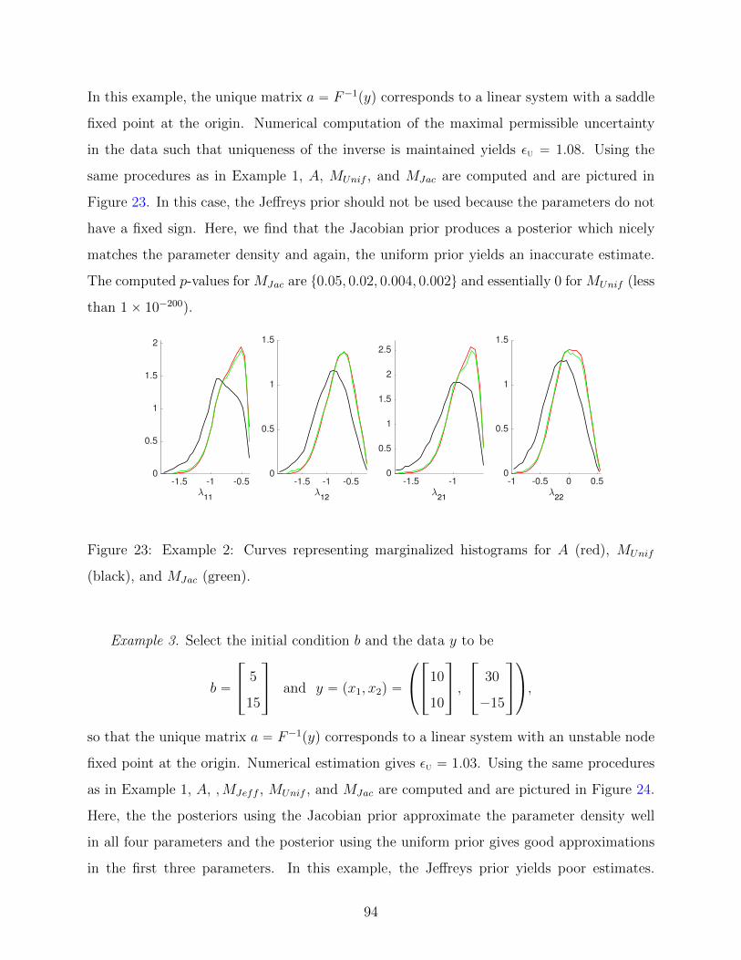
In this example, the unique matrix a “ F´1pyq corresponds to a linear system with a saddle
fixed point at the origin. Numerical computation of the maximal permissible uncertainty
in the data such that uniqueness of the inverse is maintained yields εU “ 1.08. Using the
same procedures as in Example 1, A, MUnif , and MJac are computed and are pictured in
Figure 23. In this case, the Jeffreys prior should not be used because the parameters do not
have a fixed sign. Here, we find that the Jacobian prior produces a posterior which nicely
matches the parameter density and again, the uniform prior yields an inaccurate estimate.
The computed p-values for MJac are t0.05, 0.02, 0.004, 0.002u and essentially 0 for MUnif (less
than 1ˆ 10´200).
-1.5 -1 -0.5
λ11
0
0.5
1
1.5
2
-1.5 -1 -0.5
λ12
0
0.5
1
1.5
-1.5 -1
λ21
0
0.5
1
1.5
2
2.5
-1 -0.5 0 0.5
λ22
0
0.5
1
1.5
Figure 23: Example 2: Curves representing marginalized histograms for A (red), MUnif
(black), and MJac (green).
Example 3. Select the initial condition b and the data y to be
b “
»
–
5
15
fi
fl and y “ px1, x2q “
¨
˝
»
–
10
10
fi
fl ,
»
–
30
´15
fi
fl
˛
‚,
so that the unique matrix a “ F´1pyq corresponds to a linear system with an unstable node
fixed point at the origin. Numerical estimation gives εU “ 1.03. Using the same procedures
as in Example 1, A, ,MJeff , MUnif , and MJac are computed and are pictured in Figure 24.
Here, the the posteriors using the Jacobian prior approximate the parameter density well
in all four parameters and the posterior using the uniform prior gives good approximations
in the first three parameters. In this example, the Jeffreys prior yields poor estimates.
94

The computed p-values for MJeff and MUnif are all less than 1 ˆ 10´16, and for MJac are
t0.26, 0.15, 0.22, 0.006u.
1 1.2
λ11
0
2
4
6
-0.3 -0.2 -0.1
λ12
0
2
4
6
8
-1.6 -1.4
λ21
0
2
4
6
0.3 0.4 0.5
λ22
0
2
4
6
Figure 24: Example 3: Curves representing marginalized histograms for A (red), MJeff
(blue), MUnif (black), and MJac (green).
In this series of examples, employing the Jacobian prior consistently produced good
approximations of parameter density, while accuracy resulting from using the Jeffreys and
uniform priors varied from case to case. Visual inspection of the marginals showed instances
where the uniform and Jeffreys priors seemed to give results comparable to the Jacobian
prior, however, the computed p-values indicate that the posterior sample M is most likely
to be drawn from the parameter distribution when the Jacobian prior is used.
The ability to explicitly define the data density ηpyq was ideal because it eliminated error
in the posterior estimation due to uncertainty about the available data. In applications,
experimental measurements are sparse in the data space and it is not possible to determine
the data density exactly. In the following section, we will introduce a second approach
and use it to study the accuracy of the posteriors obtained with the Jacobian prior in this
practical setting.
4.4.1.4 Comparison of priors: Approach 2 Typically, the data that will be used to
estimate the parameters of a system of ordinary differential equations are a finite collection
of experimental observations taken at incremented time intervals. The available data Y may
then be supplied as a collection of N repeated observations, ty1, y2, . . . yNu. In this case,
95

decisions must be made concerning how to represent the data in order to define the likelihood
function LpY |aq. The more accurately the data can be represented, the more reliable will
be the estimated posterior density. To study the influence of the prior in this setting, the
following approach will be used. This technique is again an adaptation of the systematic
approach described in Figure 19, while accounting for practical limitations. The following
description details our method for applying the second approach and Figure 25 provides a
corresponding schematic diagram.
1. Define a density ρpaq on the parameters.
2. Sample ρpaq to obtain A “ ta1, a2, . . . aNu, aj P A, restricting the sampling so that F is
injective on A.
3. Fix the time points for observation as t1, . . . , tn and compute the forward solution F pajq “
yj for all j, yielding the collection of simulated data Y “ ty1, y2, . . . yNu, yj P Y . Since
F : A Ñ Y is a bijection, A is, by construction, a sample of the parameter density that
we wish to approximate with the Metropolis-Hastings algorithm.
4. Use a density estimation method (such as multivariate kernel density estimation) to
represent the sample Y with a density function ηpyq.
5. Implement the Metropolis-Hastings algorithm using various priors π to obtain samples,
Mπ, of the posterior density ρpa|ηq.
6. Compare Mπ, a sample of the posterior ρpa|ηq obtained through from the Metropolis-
Hastings algorithm, to A, a sample of the parameter density.
4.4.1.5 Notes on the implementation of Approach 2 A few comments will be made
here to explain how the steps outlined in Approach 2 shall be implemented. The initial
condition b is chosen as a fixed, known value and thus the parameters of the model are the
entries of the matrix Λ. Then, a P Rn2is the parameter vector consisting of the matrix
entries of Λ. ρpaq is defined as a multivariate Gaussian distribution a „ N pa,Σq with mean
vector a and covariance matrix Σ “ σ2I where I is the n2 ˆ n2 the identity matrix. Then,
the density function is defined to be
ρpaq “1
a
p2πq4|Σ|exp
ˆ
´1
2pa´ aqJΣ´1
pa´ aq
˙
.
96

Figure 25: Visual summary of approach 2. The red coloring indicates the first density that
is defined to begin the approach. KDE refers to the kernel density estimation of Y with a
density ηpyq.
When, the sample the A “ ta1, a2, . . . aNu is randomly drawn from the density ρpaq, we
restrict to parameters for which the data is uniquely produced by that parameter (for a P A,
F paq “ y and there is no other b P A such that F pbq “ y). This can easily be achieved
in practice by selecting a mean parameter a with real, distinct eigenvalues and taking σ to
be small. Even if σ is small, aj drawn from a Gaussian distribution might fail to have real,
distinct eigenvalues, in theory. Only aj with real, distinct eigenvalues are included in the
sample. The solution map F is then used to find the corresponding data F pajq “ yj, which
yields the sample Y “ ty1, y2, . . . yNu. Due to the restriction on the sampling, it follows that
F : A Ñ Y is a bijection as desired. The value N is chosen to be large, to gain as much
information about the structure of the data density as possible.
We aim to diminish the error in the posterior sample, M , resulting from the choice of
97

how the data are represented and which likelihood function is used. In order to achieve
this objective, we seek a density function which is as close as possible to the underlying
distribution that generated the sample Y . For the finite sample of observed data, density
estimation constructs an estimate of the underlying probability density function everywhere,
including where no data are observed. Histograms are of the most simple density estimators;
however, they are not smooth and the choice of bin width leads to a constant struggle between
bias and variance [72]. Kernel density estimation is a more sophisticated alternative. In this
approach, a kernel function is centered at each data point, so that a discrete data point is
smoothed over the region surrounding it. The kernels are then summed, resulting in single
function that is the estimated density function. Background on kernel density estimation is
provided in Appendix B.
In MATLAB, the built in function ‘ksdensity’ performs a kernel density estimation for
finite sets of univariate and bivariate data. In the setting of this work, the data have
dimension nm, which will be larger than 2 in all of the following examples. MATLAB
code for multivariate kernel density estimation based on the papers [54, 55] has been made
freely available by the authors. One desirable feature of this toolbox is that the bandwidth
does not need to be prescribed and is optimally determined within the program. It can also
handle large data sets and performs a pre-clustering in order to do so. This code, with minor
modifications, was used for all density estimates presented in this work. Figure 26 shows a
4-dimensional kernel density estimate obtained using this code. In this figure, marginals of
the data are represented by blue histograms and marginals of the density estimate are given
by the red curves. The small nest of black curves depict marginals of the individual kernels
that were summed for the density estimate.
Using the same data set as Figure 26, two-dimensional projections of the data and density
estimate are given in Figure 27. In part (a), projections of the discrete data set are depicted
and in part (b), two-dimensional projections of the density estimate are shown, with the third
dimension represented by a color shading. Both of these figures indicate that the density
estimate produces an accurate representation of the data.
Returning to the implementation of Approach 2, an approximate density of sample Y is
constructed with multivariate kernel density estimation, using the freely available MATLAB
98

0 5 10
x1,1
0
0.1
0.2
0.3
-8 -6 -4 -2 0 2
x1,2
0
0.1
0.2
0.3
0.4
0 10 20
x2,1
0
0.1
0.2
-10 -5 0
x2,2
0
0.1
0.2
0.3
Figure 26: Example kernel density estimate for 4-dimensional data. Marginal histograms of
the data are shown in blue, marginals of the density estimate are given by the red curves,
and marginals of the kernels surrounding the data points are given by the black curves.
5 10
-6
-4
-2
0
x1
,2
5 10
0
5
10
15
x2
,1
-8 -6 -4 -2 00
5
10
15
5 10x
1,1
-10
-5
0
x2
,2
-6 -4 -2 0x
1,2
-10
-5
0
0 5 10 15x
2,1
-10
-5
0
(a)
5 10
-6
-4
-2
0
x1
,2
5 100
5
10
15
x2
,1
-6 -4 -2 00
5
10
15
5 10x
1,1
-10
-5
0
x2
,2
-6 -4 -2 0x
1,2
-10
-5
0
0 5 10 15x
2,1
-10
-5
0
(b)
Figure 27: Example kernel density estimate for 4-dimensional data. Two dimensional pro-
jections of the discrete data set are pictured in (a) and projections of the kernel density
estimate are given in (b).
code from [54] and is denoted by ηpyq. Next, the Metropolis-Hastings algorithm is performed
and Jeffreys prior, the uniform prior, and the Jacobian prior are employed in order to obtain
MJeff , MUnif , and MJac, respectively.
In the implementation of the Metropolis-Hastings algorithm, the density estimate ηpyq
99
will be used in the computation of the likelihood in the same manner that the exact data
density ηpyq was used in Approach 1, namely Lpη|aq “ ηpF paqq. The proposal density and
the numerical estimation of the Jacobian will be the same as presented in section 4.4.1.2.
The accuracy of the kernel density estimate reduces the error in the posterior estimate
due to incomplete knowledge of the data and the choice of likelihood, and therefore the effect
of the prior density will be revealed.
4.4.1.6 Approach 2 examples In this section, several examples of Approach 2 will be
presented in order study the accuracy of the posterior densities obtained when the Jacobian
prior is used. For ease of visualization, model (4.7) will again be restricted to the case of
two-dimensional linear systems.
Example 4. This example follows the steps outlined in Approach 2 and discussed in
section 4.4.1.5. The initial condition is fixed as b “ p10, 2qJ. The parameters are the entries
of the matrix Λ written as a vector, a “ pλ11, λ12, λ21, λ22q. The mean parameter vector used
to define ρpaq is a “ p´1,´1.5,´1,´2q, and the observation times are set as t1 “ 1 and
t2 “ 2. Here, the mean parameter value corresponds to a linear system with a stable node
equilibrium. A series of three examples is presented with increasing values for σ across all
three. The following values are used in each example: (a) σ “ 0.15, (b) σ “ 0.2, and (c)
σ “ 0.25. Y was sampled from ρpaq using N “ 5000. In Figure 28, the marginals of Y
are pictured as histograms and overlaying each is the marginalization of ηpyq drawn as a
red curve. The individual kernels, which were summed over in the density estimation, are
depicted by the (nest of) black curves. As σ increases, the spread of the data increases and
in each case, the kernel density estimate ηpyq appears to accurately represent the data.
The Metropolis-Hastings algorithm is the implemented to obtain MJeff , MUnif , and
MJac. In the same manner as the examples for Approach 1, Figure 29 displays the marginal-
ized histograms of A, MJeff , MUnif , and MJac. As before, we seek to match the red curve
which depicts A, the sample of the parameter distribution.
In part (a), MJac andAmatch very closely, whileMJeff andMUnif are quite similar to one
another, but do approximate A as well. As σ increases in parts (b) and (c), we observe that
the MJac continues to approximate A well, but the accuracy of MJeff and MUnif degrades
100

0 5 10
x1,1
0
0.1
0.3
0.5(a)
-8 -6 -4 -2 0 2
x1,2
0
0.1
0.3
0.5
0.7
0 10 20
x2,1
0
0.1
0.3
-10 -5 0
x2,2
0
0.1
0.3
0.5
0 5 10
x1,1
0
0.1
0.2
0.3
-8 -6 -4 -2 0 2
x1,2
0
0.1
0.2
0.3
0.4
0.5
0 10 20
x2,1
0
0.1
0.2
-10 -5 0
x2,2
0
0.1
0.2
0.3
0.4(b)
0 5 10
x1,1
0
0.1
0.2
0.3
-8 -6 -4 -2 0 2
x1,2
0
0.1
0.2
0.3
0.4(c)
0 10 20
x2,1
0
0.1
0.2
-10 -5 0
x2,2
0
0.1
0.2
0.3
Figure 28: Marginal histograms of Y are pictured, along with marginalizations of the density
ηpyq obtained from kernel density approximation, which are displayed as red curves. The
black curves represent the individual kernels which are summed in the density estimation.
In part (a) σ “ 0.15, (b) σ “ 0.2, and (c) σ “ 0.25, all with the same mean parameter
a “ p´1,´1.5,´1,´2q.
severely. In part (c) we finally see a difference between MJeff and MUnif with Jeffreys
performing slightly better in the last parameter. The marginals for MJeff in part (c) for the
parameters λ12 and λ21 increase near zero due to properties of Jeffreys prior. Jeffreys prior is
101

-2 -1 0λ
11
0
0.5
1
1.5
2
2.5(a)
-4 -3 -2 -1 0λ
12
0
0.5
1
1.5
2
2.5
-2 -1 0λ
21
0
0.5
1
1.5
2
2.5
-5 -4 -3 -2 -1
λ22
0
0.5
1
1.5
2
2.5
-2 -1 0λ
11
0
0.5
1
1.5
2
-4 -3 -2 -1 0
λ12
0
0.5
1
1.5
2
-2 -1 0
λ21
0
0.5
1
1.5
2
-5 -4 -3 -2 -1
λ22
0
0.5
1
1.5
2(b)
-2 -1 0
λ11
0
0.5
1
1.5
-4 -3 -2 -1 0
λ12
0
0.5
1
1.5(c)
-2 -1 0
λ21
0
0.5
1
1.5
-5 -4 -3 -2 -1
λ22
0
0.5
1
1.5
Figure 29: Curves representing marginalized histograms for A (red), MUnif (black), and
MJac (green). In part (a) σ “ 0.15, (b) σ “ 0.2, and (c) σ “ 0.25, all with the same mean
parameter a “ p´1,´1.5,´1,´2q.
uniform in the log scale and must be bounded away from zero, as an infinite likelihood occurs
there. The p-values were computed using a two-sample Kolmogorov-Smirnov test comparing
A with the various samples Mπ to determine the likelihood that the samples were drawn
from the same distribution. The p-values are reported in Table 2. They further indicate that
102

employment of the Jacobian prior produces the most accurate estimates of the parameter
density.
(a) (b) (c)
MJac t0.14, 0.63, 0.44, 0.02u t0.09, 0.51, 0.28, 0.16u t0.99, 0.05, 0.52, 0.1u
MJeff t0, 0, 0, 0u t0, 0, 0, 0u t0, 0, 0, 0u
MUnif t0, 0.0005, 0, 0u t0, 0, 0, 0u t0, 0, 0, 0u
Values less than 1ˆ 10´5 were rounded to 0.
Table 2: Two sample Kolmogorov-Smirnov test computed p-values comparing the marginals
of A with the marginals of Mπ for the parameters tλ11, λ12, λ21, λ22u.
Example 5. Choosing how to represent the available data and selecting a likelihood
function are important issues that must be confronted in order to implement the Metropolis-
Hastings algorithm. Given a collection of N observations Y “ ty1, . . . yNu, there are several
alternatives for how to represent these data. One option is to compute the mean and stan-
dard deviations at each time t1, t2, . . . , tm, denoting them by tx1, . . . , xmu and tσ1, . . . σmu,
respectively. Then the point averaged likelihood function can be defined as
LpY |aq “ź
i
Lipxi|aq
where,
Lipxi|aq “ź
j
1
σi,j?
2πe´pxjpti;aq´xi,jq
2
2σi,j2
.
Vital characteristics of the data may be lost in selecting this representation. Addition-
ally, summarizing the data in this way, inherently assumes that the data at each time point
are normally distributed, which may not be accurate. This representation of the data is
frequently used by practitioners of the Metropolis-Hastings algorithm for parameter estima-
tion.
An alternative to summarizing the data Y “ ty1, . . . yNu with these statistical quantities,
is to represent it using a multidimensional histogram. This approach is most relevant when
the system size, n, and the number of time points, m, in which the data are collected are
103

small, and the number of repeated observations, N , is large. In this case, an nm-dimensional
histogram could be used to summarize the data. If the histogram is normalized to represent
a probability density, then the likelihood function can be easily defined using the bin heights.
As is the case with one dimensional histograms, the bin widths must be prescribed and may
greatly affect the structure of the histogram. After the bin widths are selected and the
normalized histogram is constructed, it can be used to define the likelihood for use in the
Metropolis-Hastings algorithm in the following way: for a proposed parameter a, the data
F paq is computed and the histogram bin containing that data point is identified, then the
likelihood LpY |aq is the height of that bin.
As we have seen, kernel density estimation provides an accurate representation of the
data, and the likelihood is the evaluation of the estimated probability density function,
Lpη|aq “ ηpF paqq.
In Approach 2, we aimed to study the effect of the prior on the accuracy of the posterior
obtained from the Metropolis-Hastings algorithm. In order to minimize the error in posterior
due to the representation of the data, we employed kernel density estimation to define the
density ηpyq. In this example we would like to explore the effect of the choice of data rep-
resentation and likelihood function on the posteriors obtained from the Metropolis-Hastings
algorithm.
As in Example 4(a), we fix b “ p10, 2qJ, a “ p´1,´1.5,´1,´2q, tt1, t2u “ t1, 2u,
and σ “ 0.15. The data Y “ ty1, . . . yNu are constructed using N “ 10, 000 obser-
vations at times t1, 2u. Y is then represented using the three different alternatives de-
scribed above as shown in Figure 30. Here, the green curves depict the marginalized normal
density used to describe the data in the point averaged approach, with computed means
tx1,1, x1,2, x2,1, x2,2u “ t5.2,´2.4, 4.3,´2, 4u and standard deviations t0.85, 0.56, 1.41, 0.85u.
Marginalizations of the 4-dimensional histogram, constructed with 30 bins in each dimension,
are shown in yellow. Lastly, the blue curves represent the marginalized probability density
function obtained from the kernel density estimation. There is a clear discrepancy between
the point averaged and kernel density estimation representations. The Metropolis-Hastings
algorithm is then implemented with the Jacobian prior, and the appropriate likelihood func-
tion is employed in each case. Figure 31 compares the marginals of MJac computed using
104
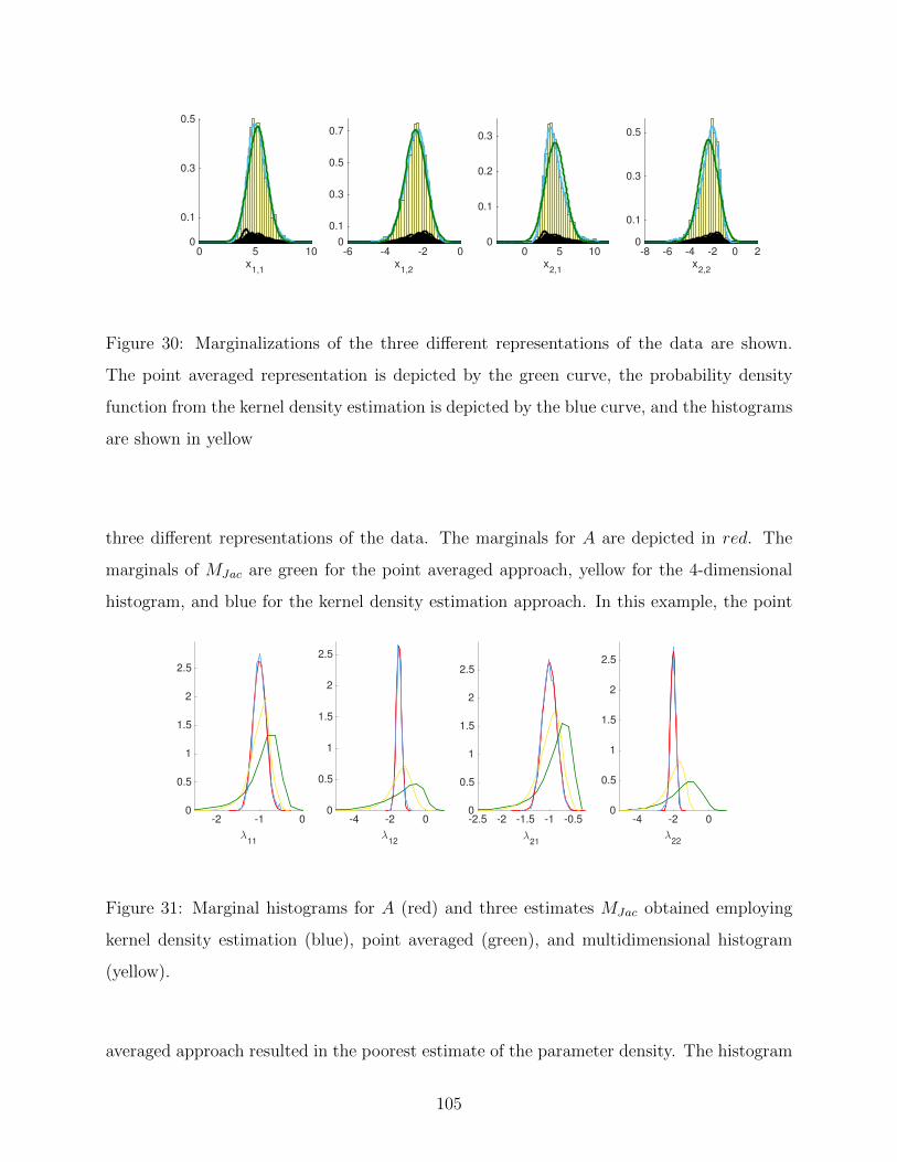
0 5 10
x1,1
0
0.1
0.3
0.5
-6 -4 -2 0
x1,2
0
0.1
0.3
0.5
0.7
0 5 10
x2,1
0
0.1
0.2
0.3
-8 -6 -4 -2 0 2
x2,2
0
0.1
0.3
0.5
Figure 30: Marginalizations of the three different representations of the data are shown.
The point averaged representation is depicted by the green curve, the probability density
function from the kernel density estimation is depicted by the blue curve, and the histograms
are shown in yellow
three different representations of the data. The marginals for A are depicted in red. The
marginals of MJac are green for the point averaged approach, yellow for the 4-dimensional
histogram, and blue for the kernel density estimation approach. In this example, the point
-2 -1 0
λ11
0
0.5
1
1.5
2
2.5
-4 -2 0
λ12
0
0.5
1
1.5
2
2.5
-2.5 -2 -1.5 -1 -0.5
λ21
0
0.5
1
1.5
2
2.5
-4 -2 0
λ22
0
0.5
1
1.5
2
2.5
Figure 31: Marginal histograms for A (red) and three estimates MJac obtained employing
kernel density estimation (blue), point averaged (green), and multidimensional histogram
(yellow).
averaged approach resulted in the poorest estimate of the parameter density. The histogram
105

approach incorporates more information than simply using means and standard deviations,
thus, as expected, the estimate of the posterior improved. The kernel density estimate clearly
provided the best estimate of A and minimized the error in the posterior estimate due to
uncertainty in the representation of the data.
4.4.2 Jacobian prior with nonlinear systems of differential equations
In this section, the use of the Jacobian prior for parameter estimation in a nonlinear system
of differential equations will be studied. The system that will be used to conduct this study
is a model for influenza A virus infection from [6]:
9V “ rI ´ cV
9H “ ´βHV
9I “ βHV ´ δI
(4.8)
where V is the concentration of infectious viral particles with units TCID50ml, H is the
number of uninfected target cells, and I is the number of productively infected cells. By
shedding viral titers, infected cells increase the concentration of viral particles at a rate
of r per cell, and free viral particles are cleared at a rate of c per day. Uninfected cells
interact with virus particles and become infected at a rate βHV . The infected cells die
at a rate of δ per cell (where 1δ is the average life span of an infected cell). The initial
number of infected cells is taken to be zero, and the initial viral concentrations, V p0q “ V0,
and initial number of target cells, Hp0q “ H0, are considered as parameters. Then, the
vector of model parameters is a “ pV0, H0, β, r, c, δq P R6 “ A, with units pTCID50ml, cells,
pTCID50mlq´1day´1, pTCID50mlqday´1,day´1,day´1q, respectively.
Approach 2 again provides a systematic way to study which prior makes the posterior a
better approximation of the parameter density. Figure 25 gives a roadmap for the approach
and the details for this specific setting are discussed here. The parameter density ρpaq is
defined to be a normal multivariate density with mean parameter vector a and covariance
matrix Σ “ diag ppa1σ1q2, pa2σ2q
2, . . . , pa6σ6q2q. In the examples below, ρpaq is constructed
by prescribing a and the vector σ “ pσ1, σ2, . . . , σ6q. As before, ρpaq is sampled to obtain
A “ ta1, a2, . . . aNu, aj P A. The number of observation times for the data will be taken
106

to be m “ 2 (so that p “ mn “ 6 and DaF paq is a square matrix). With this setup, for a
fixed a, the solution map gives, F paq “`
pV pt1q, Hpt1q, Ipt1qqJ, pV pt2q, Hpt2q, Ipt2qq
J˘
“ y.
The forward solution, F pajq “ yj, is computed for all j, yielding the collection of data
Y “ ty1, y2, . . . yNu, yj P Y . As in the previous treatment, multivariate kernel density
estimation is used to represent the sample Y with a density function ηpyq, and the Metropolis-
Hastings algorithm is implemented using various priors, to obtain Mπ. The posteriors, Mπ,
will be compared to the A, the sample of the parameter density, and to each other. A series
of four examples using this approach is now presented.
Example 6. In this example, ρpaq is constructed by selecting a “ p0.093, 4 ˆ 108, 2.7 ˆ
10´5, 0.012, 3.0, 4.0q and σ “ p0.01, 0.05, 0.01, 0.05, 0.02, 0.01q. Here, the mean parameter
values are chosen to be the average of the best-fit parameter values from [6] and σ was
prescribed to contain small values. The observation times are taken to be tt1, t2u “ t1, 2u,
and the number of samples for A and Y is N “ 1000. In Figure 32 (a), the solution to the
system for the mean parameter a is given by the blue curves, and the box plots represent
the sample of data Y , graphed at the associated time points for the corresponding variables.
The figure shows that there is a large spread in the data for this selection of σ. Part (b) of
Figure 32 shows marginal histograms of Y , and marginals of the kernel density estimate are
given by the red curves. Finally, in part (c) of the figure, A is compared to the posterior
samples MJeff , MUnif , and MJac obtained from the Metropolis-Hastings algorithm. We can
see that MJac most accurately approximates A for the parameters H0, β, r, and δ. None of
the posteriors approximate the marginals for V0 or c well. The parameter c is related to the
virus clearance; we can see from Figure 32, that for this choice of t1 and t2, the data do not
capture any information about the decay of the virus. As before, a two sample Kolmogorov-
Smirnov test was conducted, however the p-values were too small in each of the cases to
provide any useful insight in comparing MJeff , MUnif , and MJac; thus we will rely on the
marginal depictions for comparison. This will also be the case in the subsequent examples.
Example 7. In this example, everything is the same as Example 6, but the value of σ is
increased to σ “ p0.05, 0.05, 0.05, 0.1, 0.04, 0.02q for the construction of ρpaq. Figure 33 (a)
again shows the solution for the mean parameter and the box plot representations of Y . As
expected, the broadness in the spread of the data is increased. In Figure 33 (b), we compare
107

0 1 2 3 4Days
0
1
2
3
4
5
V (
TC
ID50/m
l)
×105
0 1 2 3 4Days
1
2
3
4
H (
cells
)
×108
0 1 2 3 4Days
0
5
10
15
I (c
ells
)
×107
(a)
0.09 0.095V
0
0
100
200
300
400
500(c)
3.5 4 4.5H
0 ×108
0
0.5
1
1.5
2
2.5×10
-8
2.6 2.7 2.8
β ×10-5
0
5
10
15×10
5
0.01 0.012
r
0
200
400
600
800
2.8 3 3.2
c
0
2
4
6
8
3.9 4 4.1
δ
0
2
4
6
8
10
Figure 32: Example 6: (a) Solutions curves from the mean parameter value and box plot
representations of Y . The box plots at t “ 1 for V and I are difficult to see because they
are tight relative to the figure scale. (b) marginal histograms of Y and the kernel density
estimate, (c) curves representing marginalized histograms for A (red), MJeff (blue), MUnif
(black), and MJac (green).
A, MJeff , MUnif , and MJac and see that again, MJac most accurately approximates A for the
parameters H0, β, r, and δ. In this example, there is a more pronounced discrepancy between
MUnif and MJeff and A than in Example 6. The observation times remained the same; still
no information is gathered about the decay rate of the virus, and thus the marginal for c is
not approximated well by any of the posteriors.
Example 8. In this example, different time points are chosen in an effort to obtain more
information about c. Let a and N be the same as the previous two examples, and choose
108
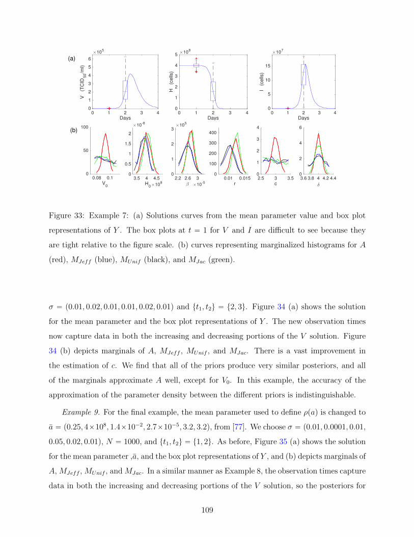
0 1 2 3 4Days
0
1
2
3
4
5
6
V (
TC
ID50/m
l)
×105
0 1 2 3 4Days
0
1
2
3
4
5
H (
cells
)
×108
0 1 2 3 4Days
0
5
10
15
I (c
ells
)
×107
(a)
0.08 0.1
V0
0
50
100(b)
3.5 4 4.5
H0×10
8
0
0.5
1
1.5
2
×10-8
2.2 2.6 3
β ×10-5
0
1
2
3×10
5
0.01 0.015
r
0
100
200
300
400
2.5 3 3.5
c
0
1
2
3
4
3.6 3.8 4 4.2 4.4
δ
0
2
4
6
Figure 33: Example 7: (a) Solutions curves from the mean parameter value and box plot
representations of Y . The box plots at t “ 1 for V and I are difficult to see because they
are tight relative to the figure scale. (b) curves representing marginalized histograms for A
(red), MJeff (blue), MUnif (black), and MJac (green).
σ “ p0.01, 0.02, 0.01, 0.01, 0.02, 0.01q and tt1, t2u “ t2, 3u. Figure 34 (a) shows the solution
for the mean parameter and the box plot representations of Y . The new observation times
now capture data in both the increasing and decreasing portions of the V solution. Figure
34 (b) depicts marginals of A, MJeff , MUnif , and MJac. There is a vast improvement in
the estimation of c. We find that all of the priors produce very similar posteriors, and all
of the marginals approximate A well, except for V0. In this example, the accuracy of the
approximation of the parameter density between the different priors is indistinguishable.
Example 9. For the final example, the mean parameter used to define ρpaq is changed to
a “ p0.25, 4ˆ108, 1.4ˆ10´2, 2.7ˆ10´5, 3.2, 3.2q, from [77]. We choose σ “ p0.01, 0.0001, 0.01,
0.05, 0.02, 0.01q, N “ 1000, and tt1, t2u “ t1, 2u. As before, Figure 35 (a) shows the solution
for the mean parameter ,a, and the box plot representations of Y , and (b) depicts marginals of
A, MJeff , MUnif , and MJac. In a similar manner as Example 8, the observation times capture
data in both the increasing and decreasing portions of the V solution, so the posteriors for
109
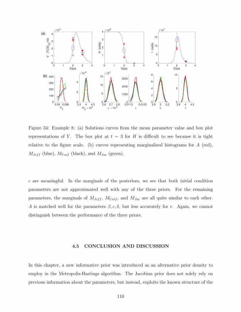
0 1 2 3 4Days
0
1
2
3
4
V (
TC
ID50/m
l)
×105
0 1 2 3 4Days
1
2
3
4
H (c
ells
)
×108
0 1 2 3 4Days
0
5
10
15
I (
cells
)
×107
(a)
0.09 0.096
V0
0
100
200
300
400
3.5 4 4.5
H0×10
8
0
2
4
×10-8
2.6 2.7 2.8
β ×10-5
0
5
10
15
×105
0.0115 0.0125
r
0
1000
2000
3000(b)
2.8 3 3.2
c
0
2
4
6
8
3.8 4 4.2
δ
0
5
10
Figure 34: Example 8: (a) Solutions curves from the mean parameter value and box plot
representations of Y . The box plot at t “ 3 for H is difficult to see because it is tight
relative to the figure scale. (b) curves representing marginalized histograms for A (red),
MJeff (blue), MUnif (black), and MJac (green).
c are meaningful. In the marginals of the posteriors, we see that both initial condition
parameters are not approximated well with any of the three priors. For the remaining
parameters, the marginals of MJeff , MUnif , and MJac are all quite similar to each other.
A is matched well for the parameters β, c, δ, but less accurately for r. Again, we cannot
distinguish between the performance of the three priors.
4.5 CONCLUSION AND DISCUSSION
In this chapter, a new informative prior was introduced as an alternative prior density to
employ in the Metropolis-Hastings algorithm. The Jacobian prior does not solely rely on
previous information about the parameters, but instead, exploits the known structure of the
110

0 1 2 3 4Days
0
200
400
600
800
1000
V (
TC
ID50/m
l)
0 1 2 3 4Days
1
2
3
4
H (c
ells
)
×108
0 1 2 3 4Days
0
0.5
1
1.5
2
I (
cells
)
×108
(a)
0.24 0.25 0.26V
0
0
50
100
150
200
3.998 4 4.002H
0 ×108
0
0.2
0.4
0.6
0.8
1×10
-5
0.0135 0.0145β
0
1000
2000
3000(b)
2.5 3p ×10
-5
0
1
2
3
4×10
5
3 3.2 3.4
c
0
2
4
6
3.1 3.2 3.3δ
0
5
10
Figure 35: Example 9: (a) Solutions curves from the mean parameter value and box plot
representations of Y . The box plot at t “ 2 for H is difficult to see because it is tight
relative to the figure scale. (b) curves representing marginalized histograms for A (red),
MJeff (blue), MUnif (black), and MJac (green).
differential equation model. This prior may not have been previously considered in the setting
of Bayesian inference, because it is specific to the problem of parameter estimation. The
model solution provides the map F , which does not appear in Bayes’ Theorem explicitly. F is
introduced in the Bayesian inference approach to parameter estimation through the likelihood
function, which makes the connection between available data and the model solution for a
given parameter.
Two systematic approaches were used to study which prior makes the posterior a better
approximation of the parameter density. In each approach, a sample of the parameter den-
sity was constructed in order to compare with the posteriors obtained by implementing the
Metropolis-Hastings algorithm with various priors. In the case of linear systems of ordinary
differential equations, we found that the Jacobian prior consistently produced better approx-
imations of the parameter density than both the uniform and Jeffreys priors. In our study
using the nonlinear influenza model, the results were less conclusive. We obtained better ap-
111

proximations of the parameter density using the Jacobian prior in two examples, and found
that the performance of the Jeffreys, Jacobian, and uniform priors was indistinguishable in
the other two examples. Analysis with additional nonlinear models is needed.
In the case of linear systems of differential equations, the theory of Chapter 3 guaranteed
the invertibility of F . In the influenza model, we were unable to verify the invertibility of
F ; some inaccuracy in the approximation may be due to this. The parameters β, r, c, δ of
model (4.8) were shown to be globally identifiable from 3 measurements of V , 2 of H, and
2 of T in [63]; however, they did not consider any initial conditions as parameters. Further
investigations are needed to determine the importance of the invertibility of F in practice.
It may be the case that local identifiability (local invertibility) is sufficient.
In this chapter, we required that p “ nm (number of parameters is equivalent to the
number of model equations multiplied by the number of observation times). This restric-
tion was imposed to ensure that the Jacobian matrix DaF paq was square. A natural next
step would be to relax this constraint and study the use of the Jacobian prior with more
observation times. In this case, a restriction of F may need to be imposed.
Finally, we note that the numerical approximation of the Jacobian determinant increases
computation time in the algorithm. For example, one iteration of the Metropolis-Hastings
algorithm with the Jacobian prior averaged 0.0225 seconds, while with the uniform and
Jeffreys priors, it was 0.01 sec.
112

5.0 CONCLUSIONS
In this work, several aspects concerning the estimation of parameters for dynamical sys-
tems using single trajectory data were addressed. The first investigation of this dissertation
confronted the question of identifiability. Specifically, we studied whether the parameters
of a linear, or linear-in-parameters, dynamical system can be uniquely determined from a
single error free trajectory of data. Several equivalent characterizations of the identifiability
criterion, were presented. For linear systems, this yielded an identifiability condition solely
based on geometric properties of the known trajectory, namely whether or not the trajectory
is confined to a proper subspace of the phase space. This criterion provides practical utility,
since it can be applied using what is known about the trajectory, without knowledge of the
structure of the parameter matrix. Several examples were presented to illustrate identifia-
bility for various systems and initial conditions. Additional results for linear systems include
a link between identifiability from single trajectory with initial condition b and the linear
independence of tb, Ab, ..., An´1bu, several characterizations of the linear independence of
tb, Ab, ..., An´1bu including a condition on the Jordan form of A. A straightforward exten-
sion was made to the case of linear-in-parameters systems, where now the geometry of the
image of the orbit in the flux space determined identifiability. Although a further extension
to the general class of nonlinear systems of differential equations would be desirable, the lack
of a unifying parameter structure within the class of these models would cause the need for
a different analytical approach than ours. We then shifted our focus to investigate identifi-
ability from a discrete collection of points along the trajectory and showed that some linear
models are identifiable from a complete trajectory but not from a finite set of data. Other
works which investigate identifiability of linear dynamical systems, typically include an input
which serves as a control for the system. Identifiability is then addressed with full access to
113
the set of all admissible controls. Our treatment is more geared toward the case of single
trajectory data. Without access to a set of controls, resulting in a variety of observations for
the system, we have only a single initial condition, and thus one trajectory, from which to
determine the parameters. This work complements this existing literature and approaches
the identifiability problem in a uniquely different way.
We continued with the theme of discrete data in Chapter 3, where we investigated the
robustness of the solution to the inverse problem. By considering a collection of data ob-
served at equally spaced time intervals along a trajectory, we sought to define the largest
allowable uncertainty in the data that could be tolerated such that properties of the inverse
solution, such as uniqueness and equilibrium stability, were maintained. We first proved that
such properties could be maintained in a neighborhood of the data, and subsequently worked
to define bounds on the maximal permissible uncertainty. Three types of bounds on uncer-
tainties were presented: analytical lower bounds, below which properties are guaranteed to
hold for all perturbations of data; analytical upper bounds, which provide proven perturba-
tions of data for which properties are guaranteed to be lost; and numerical bounds, derived
from direct sampling of data points. Our results indicate that the upper bounds, when
optimized over all potential eigenvalues, provide excellent agreement with the numerical es-
timates. All three of the bound types are hypothetically applicable to systems of arbitrary
size; however, the numerical and analytical upper bounds become computationally expen-
sive for larger systems. Although the analytical lower bound significantly underestimates
the maximal permissible uncertainty, it provides a bound that is immediately accessible for
systems of higher dimension, without increased computation. Further analysis is needed to
determine whether a more accurate analytical lower bound can be obtained using structured
perturbations. Several illustrative examples were presented and additional extensions were
developed for the case of two-dimensional linear systems. Additionally, the ability to define
the set, Cpd, εUq, on which a unique solution to the inverse problem is guaranteed at each
point, became a vital tool in the analysis conducted in Chapter 4. The results of this chap-
ter provide a useful contribution to identifiability in parameter estimation. Often, a model
can be determined to be identifiable either globally in all of parameter space or locally, in
a neighborhood of a point in parameter space. Defining the set Cpd, εUq and applying the
114

inverse map, provides an explicitly defined set in parameter space on which the model is
identifiable, that is neither an arbitrarily small neighborhood or the entire parameter space.
Additionally, our results also include bounds on regions of data space where the inverse
problem cannot be solved. The utility of such results is that they can provide an approach
for model rejection.
In Chapter 4, our focus shifts to practical aspects encountered in estimating the pa-
rameters of a dynamical system from a collection of discrete single trajectory data. In this
case, the parameter estimation problem is addressed by seeking an approximation to the
parameter density, given in the Bayesian inference approach by a posterior density. A new
informative prior was introduced as an alternative prior density to employ in the computa-
tion of the posterior with the Metropolis-Hastings algorithm. The Jacobian prior does not
solely rely on previous information about the parameters, but instead, exploits the known
structure of the differential equation model. Two systematic approaches were used to study
which prior makes the posterior a better approximation of the parameter density. In each
approach, a sample of the parameter density was constructed in order to compare with the
posteriors obtained by implementing the Metropolis-Hastings algorithm with various priors.
In the case of linear systems of ordinary differential equations, we found that the Jacobian
prior consistently produced better approximations of the parameter density than both the
uniform and Jeffreys priors. In our study using the nonlinear influenza model, the results
were less conclusive, however in our examples, that the Jacobian prior performed at least
as well as the uniform and Jeffreys priors and in a few cases, better. These findings will
be submitted as a paper to a peer-reviewed journal. This chapter provides an important
first step for introducing the use of the Jacobian prior in the Metropolis-Hastings algorithm,
however further studies are needed. An analysis with additional nonlinear models where F
is known to be invertible is our next task. A deeper look into the requirement of the injec-
tivity of F and the importance of model identifiability in practice is needed. An extension
to the case of a non-square Jacobian needs to be addressed. In this case, a restriction of F
to gain injectivity may be necessary, and defining the Jacobian as the product of nonzero
eigenvalues, may be the correct formulation in this case.
Although the models employed in this dissertation were all systems of differential equa-
115

tions, when we consider the setting of discrete data sampled from a trajectory at a sequence
of incremented time points, the systems are in fact discrete dynamical systems. There may
be more existing theory for discrete dynamical systems which can be drawn from to extend
some of our results to additional systems or classes of systems.
Throughout this work, linear systems of differential equations provided a convenient set-
ting where properties of the principal matrix solution could be exploited to develop insightful
theoretical results. The structure of these systems also allowed for an extension to nonlinear
systems which are linear in parameters. Although a system of linear equations has a simple
formulation as an ODE, the solution to the system is highly nonlinear in the parameters
and thus provides a nontrivial investigation in the setting of parameter estimation. It is
also the case that many biological systems are modeled using linear systems of differential
equations. Although the analysis of Chapter 3 is exclusive to linear systems of differential
equations, these results provided an important means to study the accuracy of the posteriors
obtained in the Metropolis-Hastings algorithm. This algorithm can be used for parameter
estimation for both linear and nonlinear differential equations. In biological modeling in
particular, Bayesian inference provides a means to represent parameter variability in a pop-
ulation. Standard parameter fitting techniques result in a single optimal parameter value as
a solution to the inverse problem; however, parameters with biological relevance are likely
to differ between individuals. Ensemble models arising from estimation of parameter den-
sities with Bayesian techniques are highly useful for biological modeling. Due to the wide
use and popularity of the Metropolis-Hastings algorithm for Bayesian parameter inference,
an advancement in improving the accuracy of the algorithm, I believe, would be the most
impactful contribution of this dissertation to the modeling community.
116

APPENDIX A
DETERMINING THE NUMBER OF REAL DISTINCT ROOTS OF A
POLYNOMIAL
A method for determining the number of real distinct roots of a polynomial was presented
by Yang [91], based on results of Gantmacher [27]. For a polynomial
pptq “ y1 ` y2t` ¨ ¨ ¨ ` yntn´1
´ tn, (A.1)
one defines the p2n` 1q ˆ p2n` 1q discrimination matrix
∆ “
»
—
—
—
—
—
—
—
—
—
—
—
—
–
´1 yn yn´1 yn´2 . . . y1 0 0 0 . . . 0
0 ´n pn´ 1qyn pn´ 2qyn´1 . . . y2 0 0 0 . . . 0
0 ´1 yn yn´1 yn´2 . . . y1 0 0 . . . 0
0 0 ´n pn´ 1qyn pn´ 2qyn´1 . . . y2 0 0 . . . 0. . .
0 0 . . . 0 0 ´1 yn yn´1 yn´2 . . . y1
fi
ffi
ffi
ffi
ffi
ffi
ffi
ffi
ffi
ffi
ffi
ffi
ffi
fl
(A.2)
comprised of alternating rows of two types.
Let Dk “detp∆1:2k,1:2kq for k “ 1, . . . , n where ∆1:2k,1:2k is the upper left 2k ˆ 2k sub-
matrix of ∆. Define sk “ signpDkq and call S “ rs1, s2, . . . , sns the sign list. If, within
S, there is some subsequence rsi`1, si`2, . . . , si`j´1s of zero entries, with j ě 3 and with
si, si`j ‰ 0, replace rsi`1, si`2, . . . , si`j´1s with r´si,´si, si, si,´si, . . . s. After all such re-
placements are made, the resulting list is termed the revised sign list.
117
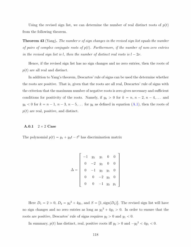
Using the revised sign list, we can determine the number of real distinct roots of pptq
from the following theorem.
Theorem 43 (Yang). The number ν of sign changes in the revised sign list equals the number
of pairs of complex conjugate roots of pptq. Furthermore, if the number of non-zero entries
in the revised sign list is l, then the number of distinct real roots is l ´ 2ν.
Hence, if the revised sign list has no sign changes and no zero entries, then the roots of
pptq are all real and distinct.
In addition to Yang’s theorem, Descartes’ rule of signs can be used the determine whether
the roots are positive. That is, given that the roots are all real, Descartes’ rule of signs with
the criterion that the maximum number of negative roots is zero gives necessary and sufficient
conditions for positivity of the roots. Namely, if yk ą 0 for k “ n, n ´ 2, n ´ 4, . . . and
yk ă 0 for k “ n´ 1, n´ 3, n´ 5, . . . for yk as defined in equation (A.1), then the roots of
pptq are real, positive, and distinct.
A.0.1 2ˆ 2 Case
The polynomial pptq “ y1 ` y2t´ t2 has discrimination matrix
∆ “
»
—
—
—
—
—
—
—
—
—
–
´1 y2 y1 0 0
0 ´2 y2 0 0
0 ´1 y2 y1 0
0 0 ´2 y2 0
0 0 ´1 y2 y1
fi
ffi
ffi
ffi
ffi
ffi
ffi
ffi
ffi
ffi
fl
Here D1 “ 2 ą 0, D2 “ y22 ` 4y1, and S “ r1, signpD2qs. The revised sign list will have
no sign changes and no zero entries as long as y22 ` 4y1 ą 0. In order to ensure that the
roots are positive, Descartes’ rule of signs requires y2 ą 0 and y1 ă 0.
In summary, pptq has distinct, real, positive roots iff y2 ą 0 and ´y22 ă 4y1 ă 0.
118

A.0.2 3ˆ 3 Case
The polynomial pptq “ y1 ` y2t` y3t2 ´ t3 has discrimination matrix
∆ “
»
—
—
—
—
—
—
—
—
—
—
—
—
—
—
—
–
´1 y3 y2 y1 0 0 0
0 ´3 2y3 y2 0 0 0
0 ´1 y3 y2 y1 0 0
0 0 ´3 2y3 y2 0 0
0 0 ´1 y3 y2 y1 0
0 0 0 ´3 2y3 y2 0
0 0 0 ´1 y3 y2 y1
fi
ffi
ffi
ffi
ffi
ffi
ffi
ffi
ffi
ffi
ffi
ffi
ffi
ffi
ffi
ffi
fl
Here D1 “ 3 ą 0, D2 “ 2y23 ` 6y2, D3 “ ´27y2
1 ´ p4y33 ` 18y2y3qy1 ` 4y3
2 ` y22y
23, and
S “ r1, signpD2q, signpD3qs. The revised sign list will have no sign changes and no zero entries
as long as D2 ą 0 and D3 ą 0. In order to ensure that the roots are positive, Descartes’ rule
of signs requires y3 ą 0, y2 ă 0, and y1 ą 0.
In summary, pptq has distinct, real, positive roots iff y3 ą 0, ´y32 ă 3y2 ă 0, and
maxp0,´b ´ 2?Cq ă 27y1 ă ´b ` 2
?C, where b “ 2y3
3 ` 9y2y3 and C “ y63 ` 9y2y
43 `
27y22y
23 ` 27y3
2.
119

APPENDIX B
KERNEL DENSITY ESTIMATION
For a finite sample of observed data, density estimation constructs an estimate of the un-
derlying probability density function everywhere, including where no data are observed.
Histograms are of the most simple density estimators; however, they are not smooth and
the choice of bin width leads to a constant struggle between bias and variance [72]. Kernel
density estimation is a more sophisticated alternative. In this approach, a kernel function is
centered at each data point, so that a discrete data point is smoothed over the region sur-
rounding it. The kernels are then summed, resulting in single function that is the estimated
density function.
A kernel density estimation in one dimension is depicted in Figure 36 (a). The discrete
collection of data points are plotted as stars along the x-axis and the individual kernels are
pictured in blue. The density estimate resulting from summing these kernels is represented
by the black curve. The case of kernel density estimation in two dimensions is pictured in
Figures 36 (b) and (c) as presented in [72]. The contours represent the individual kernels
surrounding the data points in part (b), and the resulting density estimate in part (c).
The mathematical formulation for the multivariate kernel density estimation is as follows:
Given n data points w1, w2, . . . wn in Rd, the estimated density function is given by
fHpwq “1
n
nÿ
i“1
KHpw ´ wiq.
120

-10 0 10 20 30 40x
0
0.01
0.02
0.03
0.04
0.05
0.06D
en
sity
(a) (b) (c)
Figure 36: Kernel density estimation in (a) one dimension, and (b), (c) two dimensions.
The bandwidth matrix, H P Rdˆd, is symmetric positive definite.
KHpwq “ |H|´12KpH´12wq,
where Kpwq is the kernel function. The standard multivariate normal kernel Kpwq “
p2πq´d2 expp´12wTwq is often employed, however other kernel functions are also used. Selec-
tion of the bandwidth matrix is the most important task as it controls the orientation and
the amount of smoothing and thus the accuracy of the density estimate [71].
121

BIBLIOGRAPHY
[1] A. H. Al-Mony and N. J. Higham, Improved inverse scaling and squaring algorithmsfor the matrix logarithm, SIAM Journal on Sci. Comp., 34 (2012), pp. C153–C169.
[2] R. C. Allen and S. A. Pruess, An analysis of an inverse problem in ordinarydifferential equations, SIAM J. Sci. Stat. Comput. 2 (1981), pp. 176–185.
[3] L. J. S. Allen, An Introduction to Stochastic Processes with Applications to Biology,Taylor and Francis Group, 2011.
[4] L. J. S. Allen, Matrix Analysis, Taylor and Francis Group, 2011.
[5] K. J. Astrom and P. Eykhoff, System identification–a survey, Automatica J. IFAC,7 (1971), pp. 123–162.
[6] P. Baccam, C. Beauchemin, C. A. Macken, F. G. Hayden, and A. S. Perel-son, Kinetics of influenza A virus infection in humans, J. of Virol., 80 (2006), pp. 7590–7599.
[7] D. Battogtokh, D. K. Asch, M. E. Case, J. Arnold, and H. B. Schuttler,An ensemble method for identifying regulatory circuits with special reference to the qagene cluster of Neurospora crassa, PNAS, 99 (2002), pp. 16904–16909.
[8] R. Bellman and K. J. Astrom, On structural identifiability, Math. Biosci., 7 (1970),pp. 329–339.
[9] G. Bellu, M. P. Saccomani, S. Audoly, L. D’Angio, DAISY: a new softwaretool to test global identifiability of biological and physiological systems, Comput. Meth.Programs Biomed., 88 (2007), pp. 52–61.
[10] K. J. Berger, The case for objective Bayesian analysis, Bayesian Analysis, 1 (2006),pp. 385–402.
[11] P. L. Bonate, Pharmacokinetic-Pharmacodynamic Modeling and Simulation, Springer,New York, 2006.
[12] H. G. Bock, Recent advances in parameter identification for ordinary differential equa-tions, Progress in Scientific Computing 2, (1983), pp. 95–121.
122

[13] L. Chen and G. Bastin, Structural identifiability of the yield coefficients in bioprocessmodels when the reaction rates are unknown, Math. Biosci., 132 (1996), pp. 35–67.
[14] S. H. Hun and N. J. Higham and C. S. Kenney and A. J. Laub, Approximatingthe logarithm of a matrix to specified accuracy, SIAM Journal on Matrix Analysis andApplications, 22 (2001), pp. 1112–1125.
[15] C. Cobelli and J. J. DiStefano, Parameter and structural identifiability conceptsand ambiguities: A critical review and analysis, Am. J. Physiol., 239 (1980), pp. R7–R24.
[16] G. Craciun and C. Pantea, Identifiability of chemical reaction networks, J. Math.Chem., 44 (2008), pp. 244–259.
[17] W. J. Culver, On the existence and uniqueness of the real logarithm of a matrix, Proc.Amer. Math. Soc., 17 (1966), pp. 1146–1151.
[18] J. DiStefano III and C. Cobelli, On parameter and structural identifiability:Nonunique observability/reconstructibility for identifiable systems, other ambiguities,and new definitions, IEEE Trans. Automat. Control, 25 (1980), pp. 820–833.
[19] S. Daun, J. Rubin, Y. Vodovotz, G. Clermont, Equation-based models of dy-namic biological systems, J. of Crit. Care, 23 (2008), pp. 585–594.
[20] D. J. Earl and M. W. Deem, Parallel tempering: Theory, applications, and newperspectives, Phys. Chem. Chem. Phys., 7 (2005), pp. 3910–3916.
[21] L. Edelstein-Keshet, Mathematical Models in Biology, Classics Appl. Math. 46,SIAM, Philadelphia, 2005. Unabridged republication of the work first published by Ran-dom House, New York, 1988.
[22] F. Fairman, Linear Control Theory: The State Space Approach, Wiley, New York,1998.
[23] M. Farina, R. Findeisen, E. Bullinger, S. Bittanti, F. Allgower, andP. Wellstead, Results towards identifiability properties of biochemical reaction net-works, in Proceedings of the 45th IEEE Conference on Decision and Control, IEEEPress, Piscataway, NJ, 2006, pp. 2104–2109.
[24] M. Feinberg, Chemical reaction network structure and the stability of complex isother-mal reactors-I. The deficiency zero and deficiency one theorems, Chem. Engrg. Sci., 42(1987), pp. 2229–2268.
[25] M. Feinberg, The existence and uniqueness of steady states for a class of chemicalreaction networks, Arch. Ration. Mech. Anal., 132 (1995), pp. 311–370.
[26] G. B. Folland, Real Analysis, Modern Techniques and their Applications, Wiley-Interscience, 1984.
123

[27] F. R. Gantmacher, The Theory of Matrices: Vol. 2, The theory of matrices Series.Chelsea, 1974.
[28] B. C. Gargash and D. P. Mital, A necessary and sufficient condition of global struc-tural identifiability of compartmental models, Comput. Biol. Med., 10 (1980), pp. 237–242.
[29] A. Gelman, J. Carlin, H. Stern, and D. Rubin, Bayesian Data Analysis, SecondEdition, London: Chapman and Hall, 2004.
[30] K. Glover and J. Willems, Parametrizations of linear dynamical systems: Canon-ical forms and identifiability, IEEE Trans. Automat. Control, 19 (1974), pp. 640–646.
[31] K. Godfrey, Compartmental Models and their Application, Academic Press, 1983.
[32] M. Goldstein, Subjective Bayesian analysis: principles and practice, Bayesian Anal-ysis, 3 (2006), pp. 403–420.
[33] P. C. Gregory, Bayesian Logical Data Analysis for the Physical Sciences, CambridgeUniversity Press, 2005.
[34] M. Grewal and K. Glover, Identifiability of linear and nonlinear dynamical sys-tems, IEEE Trans. Automat. Control, 21 (1976), pp. 833–837.
[35] W. K. Hastings, Monte Carlo sampling methods using Markov chains and their ap-plications, Biometrika, 57 (1970), pp. 97–109.
[36] F. G. Hayden, J. J. Treanor, R. F. Betts, M. Lobo, J. D. Esinhart, andE. K. Hussey, Safety and efficacy of the neuraminidase inhibitor GG167 in experi-mental human influenza, JAMA, 275 (1996), pp. 295–299.
[37] N. J. Higham, Functions of matrices: theory and computation, Chapter 11, SIAM,2008.
[38] D. M. Himmelblau, C. R. Jones, and K. B. Bischoff, Determination of rateconstants for complex kinetics models, Indust. Engrg. Chem. Fund., 6 (1967), pp. 539–543.
[39] D. Hinrichsen and A. J. Pritchard, Mathematical Systems Theory I, Modelling,State Space Analysis, Stability and Robustness, Springer-Verlag, 2005.
[40] K. Hoffman and R. Kunze, Linear Algebra, Prentice–Hall, Englewood Cliffs, NJ,1971.
[41] F. Horn and R. Jackson, General mass action kinetics, Arch. Ration. Mech. Anal.,47 (1972), pp. 81–116.
124

[42] R. A. Horn and C. R. Johnson, Matrix Analysis, Cambridge University Press, NewYork, 1990.
[43] B. P. Ingalls, Mathematical Modeling in Systems Biology: An Introduction, MITPress, Cambridge, MA, 2013.
[44] J. Jacquez and P. Greif, Numerical parameter identifiability and estimability: in-tegrating identifiability, estimability, and optimal sampling design, Math. Biosci., 77(1985), pp. 201–227.
[45] H. Jeffreys, Theory of Probability, Oxford: Clarendon Press, 1961.
[46] A. Kadioglu, N. A. Gingles, K. Grattan, A. Kerr, T. J. Mitchell, andP. W. Andrew, Host cellular immune response to pneumococcal lung infection inmice, Infect. Immun., 68 (2000), pp. 492–501.
[47] T. Kailath, Linear Systems, Prentice–Hall, Englewood Cliffs, NJ, 1980.
[48] R. E. Kalman, Mathematical description of linear dynamical systems, J. Soc. Indust.Appl. Math. Ser. A Control, 1 (1963), pp. 152–192.
[49] R. E. Kalman, A new approach to linear filtering and prediction problems, Trans.ASME J. Basic Engineering, 82 D (1960), pp. 35-45.
[50] A. V. Karnaukhov, E. V. Karnaukhova, and J. R. Williamson, Numericalmatrices method for nonlinear system identification and description of dynamics of bio-chemical reaction networks, Biophys. J., 92 (2007), pp. 3459–3473.
[51] C. T. Kelley, Iterative Methods for Optimization, Vol 18, SIAM, 1999.
[52] B. Kisacanin and G. C. Agarwal, Linear Control Systems: With Solved Problemsand MATLAB Examples, Kluwer Academic/Plenum Publishers, New York, 2001.
[53] H. Kitano, Systems biology: a brief overview, Science, 295 (2002), pp. 1662–1664.
[54] M. Kristan, A. Leonardis, and D. Skocaj, Multivariate online kernel densityestimation with Gaussian kernels, Pattern Recognition, 44 (2011), pp. 2630–2642.
[55] M. Kristan, D. Skocaj, and A. Leonardis, Online kernel density estimation forinteractive learning, Image and Vision Computing, 28 (2010), pp. 1106–1116.
[56] R. C. K. Lee, Optimal Estimation, Identification, and Control, Research Monographs196, MIT Press, Cambridge, MA, 1964.
[57] G. Lillacci and M. Khammash, Parameter estimation and model selection in com-putational biology, PLoS Comp. Bio., 6 (2010), e1000696.
[58] L. Ljung and T. Glad, On global identifiability for arbitrary model parametrizations,Automatica J. IFAC, 30 (1994), pp. 265–276.
125

[59] S. Lukens, J. DePasse, R. Rosenfeld, E. Ghedin, E. Mochan, S. T. Brown,J. Grefenstette, D. S. Burke, D. Swigon, and G. Clermont, A large-scaleimmuno-epidemiological simulation of influenza A epidemics, BMC Public Health, 14(2014), 1019.
[60] F. Mazzocchi, Complementarity in biology, EMBO Reports, 11 (2010), pp. 339–344.
[61] N. Metropolis, A. W. Rosenbluth, M. N. Rosenbluth, A. H. Teller andE. Teller, Equation of state calculations by fast computing machines, The journal ofchemical physics, 21 (1953), pp. 1087–1092.
[62] J. A. McCullers, J. L. McAuley, S. Browall, A. R. Iverson, K. L. Boyd,and B. Henriques-Normark, Influenza enhances susceptibility to natural acquisitionof and disease due to Streptococcus pneumoniae in ferrets, J. Infect. Dis., 202 (2010),pp. 1287–1295.
[63] H. Miao, X. Xia, A. S. Perelson, and H. Wu, On identifiability of nonlinear ODEmodels and applications in viral dynamics, SIAM Rev., 53 (2011), pp. 3–39.
[64] E. Mochan, D. Swigon, G. B. Ermentrout, S. Lukens, and G. Clermont, Amathematical model of intrahost pneumococcal pneumonia infection dynamics in murinestrains, J. of Theor. Biol., 353 (2014), pp. 44–54.
[65] E. Mochan-Keef, D. Swigon, G. B. Ermentrout, and G. Clermont, A three-tiered study of differences in murine intrahost immune response to multiple pneumococcalstrains, PloS one, 10 (2015), e1034012.
[66] J. D. Murray, Mathematical Biology I: An Introduction, Interdiscip. Appl. Math. 17,Springer, New York, 2002.
[67] V. V. Nguyen and E. F. Wood, Review and unification of linear identifiabilityconcepts, SIAM Rev., 24 (1982), pp. 34–51.
[68] S. J. Press, Subjective and objective Bayesian Statistics: Principles, Models, and Ap-plications, LibreDigital, 2003.
[69] I. Price, E. D. Mochan-Keef, D. Swigon, G. B. Ermentrout, S. Lukens,F. R. Toapanta, T. M. Ross, and G. Clermont, The inflammatory response toinfluenza A virus (H1N1): an experimental and mathematical study, J. of Theor. Biol.,374 (2015), pp. 44–54.
[70] H. H. Rosenbrock, Structural properties of linear dynamical systems, Int. J. Control,20 (1974), pp. 191–202.
[71] D. W. Scott and S. R. Sain, 9-Multi-dimensional density estimation, Handbook ofstatistics 24 (2005), pp. 229–261.
[72] J. S. Simonoff, Smoothing Methods in Statistics, Springer-Verlag New York, 1996.
126

[73] B. Singer and S. Spilerman, The representation of social processes by Markov mod-els, Am. J. of Soc. 82, 1 (1976), pp. 1–54.
[74] R. C. Smith, Uncertainty Quantification: Theory, Implementation, and Applications,SIAM, Philadelphia, 2014.
[75] E. D. Sontag, For differential equations with r parameters, 2r + 1 experiments areenough for identification, J. Nonlinear Sci., 12 (2002), pp. 553–583.
[76] S. Stanhope and J. E. Rubin and D. Swigon, Identifiability of Linear and Linear-in-Parameters Dynamical Systems from a Single Trajectory, SIAM J. on Appl. Dynam.Syst., 13 (2014), pp. 1792–1815.
[77] D. Swigon, Ensemble modeling of biological systems, in Mathematics and Life Sciences,Eds. A.V. Antoniouk and R.V.N. Melnik, De Gruyter (2012), pp. 19–42.
[78] M. Tanner, Tools for Statistical Inference, Second Edition, Springer-Verlag, New York,1993.
[79] A. Tarantola, Inverse Problem Theory and Methods for Model Parameter Estimation,SIAM, Philadelphia, 2005.
[80] A. Thowsen, Identifiability of dynamic systems, Int. J. Systems Sci., 9 (1978), pp. 813–825.
[81] L. Tierney, Markov chains for exploring posterior distributions An. of Stat., 22 (1994),pp. 1701–1762.
[82] F. R. Toapanta and T. M. Ross, Impaired immune responses in the lungs of agedmice following influenza infection, Respir. Res., 10 (2009), pp. 112–131.
[83] L. N. Trefethen and D. Bau III, Numerical Linear Algebra, SIAM, Philadelphia,1997.
[84] S. Vajda, P. Valko, and A. Yermakova, A direct-indirect procedure for estimationof kinetic parameters, Comput. Chem. Engrg., 10 (1986), pp. 49–58.
[85] B. Van Domselaar and P. W. Hemker, Nonlinear parameter estimation in initialvalue problems, Stitching Mathematisch Centrum, 1975.
[86] M. H. V. Van Regenmortel, Reductionism and complexity in molecular biology,EMBO Reports, 5 (2004), 1016-1020.
[87] H. U. Voss, J. Timmer, and J. Kurths, Nonlinear dynamical system identificationfrom uncertain and indirect measurements, Int. J. of Bifurcation and Chaos, 14 (2004),pp. 1905–1933.
127

[88] E. Walter, Y. Lecourtier, and J. Happel, On the structural output distinguisha-bility of parametric models, and its relations with structural identifiability, IEEE Trans.Automat. Control, 29 (1984), pp. 56–57.
[89] E. Walter and L. Pronzato, Identification of Parametric Models from ExperimentalData, translated from the 1994 French original and revised by the authors, with the helpof John Norton, Comm. Control Engrg. Ser., Springer-Verlag, Berlin, Masson, Paris,1997.
[90] X. Xia and C. H. Moog, Identifiability of nonlinear systems with applications toHIV/AIDS models, IEEE Trans. Automat. Control, 48 (2003), pp. 330–336.
[91] L. Yang, Recent Advances on determining the number of real roots of parametric poly-nomials, J. Symb. Comp., 28 (1999) pp. 225–242.
[92] S. Yousef, Iterative Methods for Sparse Linear Systems, 2nd ed., SIAM, Philadelphia,2003.
128