PARAMETER ESTIMATION IN A DIAGNOSTIC WIND MODEL … · Grassland, Forest, Scrubs, No Vegetation, Arti cial Coverage, Wet Coverage and Water Coverage) ... PST Grasslands 0:09 0:001{0:15

6th European Conference on Computational Mechanics (ECCM 6)7th European Conference on Computational Fluid Dynamics (ECFD 7)

1115 June 2018, Glasgow, UK

PARAMETER ESTIMATION IN A DIAGNOSTIC WINDMODEL OVER COMPLEX TERRAIN

G. Montero1, E. Rodrıguez1, A. Oliver1 and J. Calvo2

1 SIANI - University of Las Palmas de Gran Canaria, Edificio Polivalente I, CampusUniversitario de Tafira, Las Palmas de Gran Canaria, Spain, (gustavo.montero,

eduardo.rodriguez, albert.oliver)@ulpgc.es,http://www.dca.iusiani.ulpgc.es/proyecto2015-2017/html/index.html

2 Agencia Estatal de Meteorologıa (AEMET), Leonardo Prieto Castro, 8, 28040-Madrid,Spain, [email protected], www.aemet.es

Key words: Parameter Estimation, Wind Modelling, Roughness Parameters, MemeticAlgorithms

Abstract. The aerodynamic roughness length (z0) and the displacement height (d) arecritical for wind modelling based on the log vertical profile. It is well known that thevalues of these parameters depend on weather conditions and land coverage. Thus, manyauthors have studied its relationship, providing typical ranges for each land coverage. Inthis work, a comprehensive literature review is performed to collect the ranges of z0 andd for each surface type. In particular, we have focused on the coverages present in theInformation System of Land Cover of Spain (SIOSE) [1]. Using these ranges, we proposea procedure to construct z0 and d maps through a downscaling wind model. Results fromthe HARMONIE-AROME and ECMWF mesoscale numerical weather prediction modelsare downscaled using a 3D diagnostic wind model with adaptive finite element method[2, 3]. The values of z0 and d are estimated with a memetic algorithm that combines theDifferential Evolution method [4], a rebirth operator and the L-BFGS-B algorithm [5]. So,the root mean square error (RMSE) of the wind model is minimised against the observedwind data. This fast procedure allows updating the roughness parameters for any weathercondition. Some numerical experiments are presented to show the performance of thismethodology. Although we work with the SIOSE database and the Wind3D model, themethod can be used in conjunction with other databases and downscaling models.

1 INTRODUCTION

The influence of aerodynamic parameters in the modelling of wind field in the mi-croscale and mesoscale, specially the wind velocity near the ground, is well known. There-fore, the accuracy of these parameters is critical to simulate the wind field used in windpower plants energy prediction, dispersion of air pollution, and wildland fire spread amongothers. In this paper we propose a strategy to improve the results of a downscaling wind

G. Montero, E. Rodrıguez, A. Oliver and J. Calvo

model by estimating the values of the roughness length (z0) and displacement height (d)using Differential Evolution (DE) and a rebirth operator (RO).

A downscaling wind model uses the prediction of a Numerical Weather Prediction(NWP) model as input wind field to compute a new one in a higher resolution meshthat better captures the terrain features. In this paper, the downscaling wind modelis Wind3D [3], a diagnostic mass-consistent wind model with an updated atmosphericparameterisation and wind profile proposed in [6, 7, 8], and it is coupled with two differentNWP models: specifically the European Centre for Medium-Range Weather Forecasts(ECMWF) model [9] and the HARMONIE-AROME model [10]. In this paper we haveused the land cover database of Spain (SIOSE) [1].

The content of the paper is organised as follows. As a first step, we need to know thedifferent land covers of the region that, in this case, are given by the SIOSE databasedescribed in Sect. 2. Then, we identify the suitable ranges of z0 and d for each land cover;these ranges are given in the literature and shown in Sect. 3. For a given region thereexists a combination of different land covers, so we need to compute the actual value ofeach aerodynamic parameter by using the formula presented in Sect. 3 too. Then, withthese values and the forecast wind field of the NWP model, we simulate the resultingwind field with the Wind3D model (Sect. 4). The last step of the algorithm is to computethe fitting function (the root square mean error between the predicted and the observedwind in meteorological stations) and generate the next population of the optimisationalgorithm (Sect. 5). Numerical experiments in a realistic case in Gran Canaria Island aredescribed in Sect. 6. Finally, the conclusions of this work are summed up in Sect. 7.

2 SIOSE LAND COVER DATABASE

In 1990, the first land cover database encompassing the whole national territory wasconstructed in Spain on a scale of 1 : 100.000. It was developed in the framework of theCORINE Land Cover (CLC) European project [11]. After successive updates in 2000,2006 and 2012, it became Image & CORINE Land Cover. The SIOSE database consistsof different basic (40) and compound coverages. A compound coverage is made up of acombination of basic ones. It considers eight general groups of basic coverages (Crops,Grassland, Forest, Scrubs, No Vegetation, Artificial Coverage, Wet Coverage and WaterCoverage) that are further refined into forty specific classes of basic coverage; see [12].

3 ROUGHNESS LENGTH AND DISPLACEMENT HEIGHT

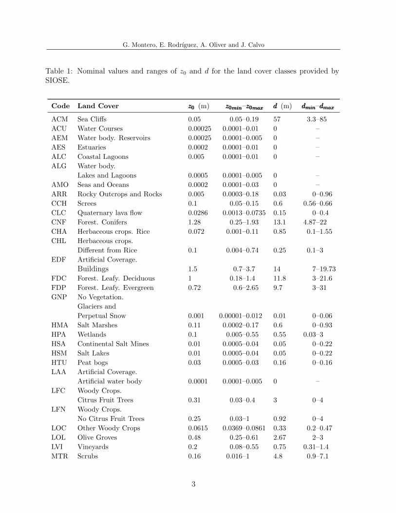
To obtain siutable values of z0 and d, we must define the search space of them. Wehave carried out a literature review to find the ranges of z0 and d values showed in Table 1for each land cover; see [3]. The first and second columns show the SIOSE code and adescription for each land coverage. The third and fourth, and the fifth and sixth columnspresent the nominal value and the range of the parameters z0 and d, respectively.

The SIOSE project uses a vectorial format, but, for convenience, we will translate itto a raster format. For this, we will define a grid with np points and, for each point, wewill look for the mean value of basic coverages. Once we have the values of z0 and d for

2


Table 1: Nominal values and ranges of z0 and d for the land cover classes provided bySIOSE.

Code Land Cover z0z0z0 (m) z0minz0minz0min–z0maxz0maxz0max ddd (m) dmindmindmin–dmaxdmaxdmax

ACM Sea Cliffs 0.05 0.05–0.19 57 3.3–85

ACU Water Courses 0.00025 0.0001–0.01 0 –AEM Water body. Reservoirs 0.00025 0.0001–0.005 0 –AES Estuaries 0.0002 0.0001–0.01 0 –ALC Coastal Lagoons 0.005 0.0001–0.01 0 –ALG Water body.

Lakes and Lagoons 0.0005 0.0001–0.005 0 –AMO Seas and Oceans 0.0002 0.0001–0.03 0 –ARR Rocky Outcrops and Rocks 0.005 0.0003–0.18 0.03 0–0.96

CCH Screes 0.1 0.05–0.15 0.6 0.56–0.66

CLC Quaternary lava flow 0.0286 0.0013–0.0735 0.15 0–0.4

CNF Forest. Conifers 1.28 0.25–1.93 13.1 4.87–22

CHA Herbaceous crops. Rice 0.072 0.001–0.11 0.85 0.1–1.55

CHL Herbaceous crops.

Different from Rice 0.1 0.004–0.74 0.25 0.1–3

EDF Artificial Coverage.

Buildings 1.5 0.7–3.7 14 7–19.73

FDC Forest. Leafy. Deciduous 1 0.18–1.4 11.8 3–21.6

FDP Forest. Leafy. Evergreen 0.72 0.6–2.65 9.7 3–31

GNP No Vegetation.

Glaciers and

Perpetual Snow 0.001 0.00001–0.012 0.01 0–0.06

HMA Salt Marshes 0.11 0.0002–0.17 0.6 0–0.93

HPA Wetlands 0.1 0.005–0.55 0.55 0.03–3

HSA Continental Salt Mines 0.01 0.0005–0.04 0.05 0–0.22

HSM Salt Lakes 0.01 0.0005–0.04 0.05 0–0.22

HTU Peat bogs 0.03 0.0005–0.03 0.16 0–0.16

LAA Artificial Coverage.

Artificial water body 0.0001 0.0001–0.005 0 –LFC Woody Crops.

Citrus Fruit Trees 0.31 0.03–0.4 3 0–4

LFN Woody Crops.

No Citrus Fruit Trees 0.25 0.03–1 0.92 0–4

LOC Other Woody Crops 0.0615 0.0369–0.0861 0.33 0.2–0.47

LOL Olive Groves 0.48 0.25–0.61 2.67 2–3

LVI Vineyards 0.2 0.08–0.55 0.75 0.31–1.4

MTR Scrubs 0.16 0.016–1 4.8 0.9–7.1

3


Table 1: Continued

Code Land Cover z0 (m)z0 (m)z0 (m) z0minz0minz0min–z0maxz0maxz0max d (m)d (m)d (m) dmindmindmin–dmaxdmaxdmax

OCT Artificial Coverage.

Other Buildings 0.5 0.06–1 4 2–14

PDA No Vegetation.

Beaches, Dunes and Sandy Areas 0.0003 0.0003–0.06 0 0–0.33

PRD Crops. Meadows 0.03 0.001–0.1 0.013 0.007–0.035

PST Grasslands 0.09 0.001–0.15 0.171 0.013–0.66

RMB No Vegetation. Ravines 0.0012 0.0003–0.005 0.03 0–0.03

SDN No Vegetation. Bare Soil 0.001 0.0002–0.04 0.03 0–0.22

SNE Artificial Coverage.

Unbuilt Land 0.0003 0.0002–0.04 0 0–0.22

VAP Artificial Coverage.

Road, Parking or Unvegetated

Pedestrian Areas 0.03 0.0035–0.5 1 0.02–2.5

ZAU Artificial Coverage.

Artificial Green Area and

Urban Trees 0.4 0.03–1.3 3.5 3.5–14

ZEV Artificial Coverage.

Extraction or Waste Areas 0.1 0.0003–0.18 0.16 0–1

ZQM No Vegetation. Burnt Areas 0.6 0.1–1.1 3.27 0.54–6

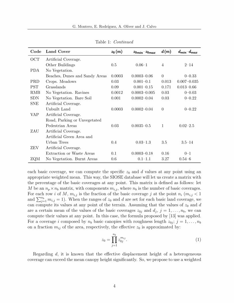
each basic coverage, we can compute the specific z0 and d values at any point using anappropriate weighted mean. This way, the SIOSE database will let us create a matrix withthe percentage of the basic coverages at any point. This matrix is defined as follows: letM be an np×nb matrix, with components mi,j, where nb is the number of basic coverages.For each row i of M , mi,j is the fraction of the basic coverage j at the point ni (mi,j < 1and

∑nbj=1mi,j = 1). When the ranges of z0 and d are set for each basic land coverage, we

can compute its values at any point of the terrain. Assuming that the values of z0 and dare a certain mean of the values of the basic coverages z0j and dj, j = 1, . . . , nb, we cancompute their values at any point. In this case, the formula proposed by [13] was applied.For a coverage i composed by nb basic canopies with roughness length z0j; j = 1, . . . , nbon a fraction mij of the area, respectively, the effective z0 is approximated by:

z0 =

nb∏j=1

zmij0j . (1)

Regarding d, it is known that the effective displacement height of a heterogeneouscoverage can exceed the mean canopy height significantly. So, we propose to use a weighted

4


root mean square to obtain a higher mean value than Taylor’s one:

d =

√√√√ nb∑j=1

mijd2j , (2)

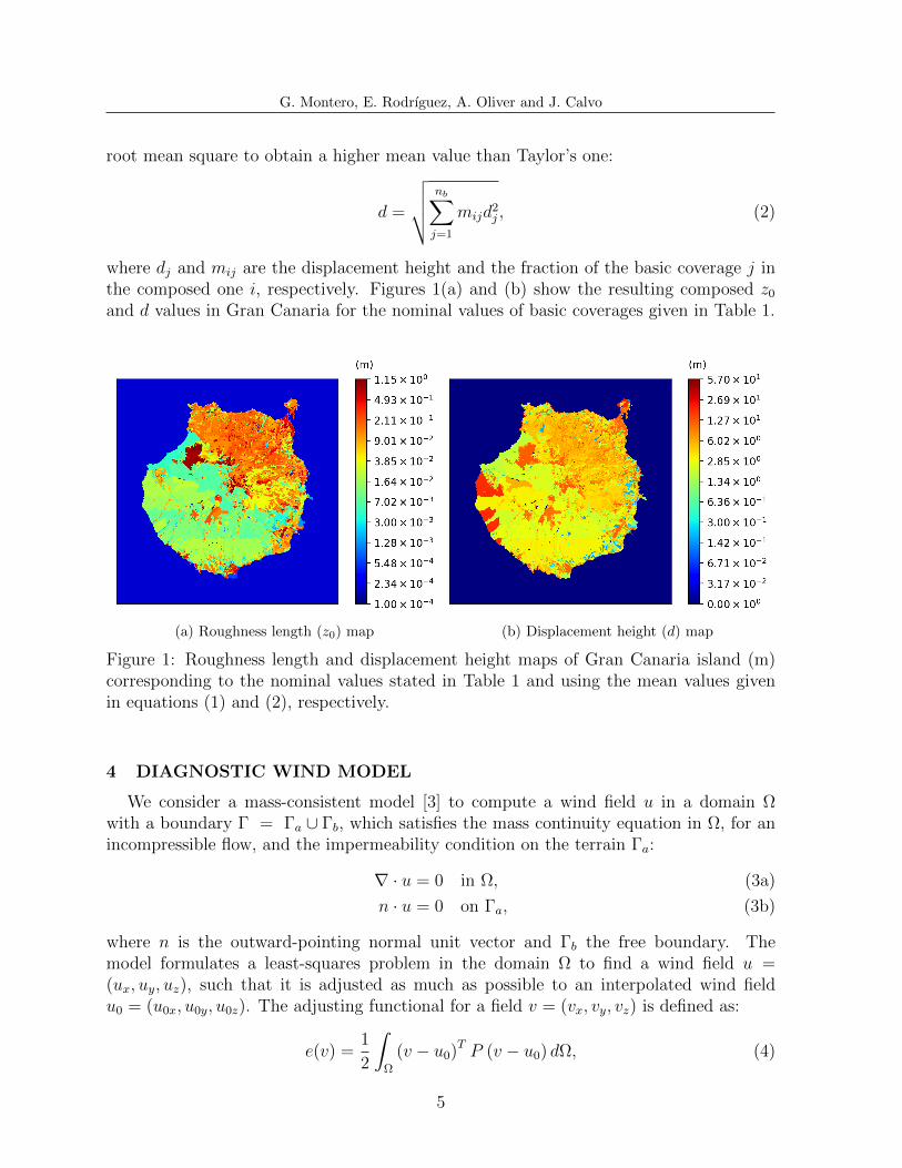
where dj and mij are the displacement height and the fraction of the basic coverage j inthe composed one i, respectively. Figures 1(a) and (b) show the resulting composed z0

and d values in Gran Canaria for the nominal values of basic coverages given in Table 1.

(a) Roughness length (z0) map (b) Displacement height (d) map

Figure 1: Roughness length and displacement height maps of Gran Canaria island (m)corresponding to the nominal values stated in Table 1 and using the mean values givenin equations (1) and (2), respectively.

4 DIAGNOSTIC WIND MODEL

We consider a mass-consistent model [3] to compute a wind field u in a domain Ωwith a boundary Γ = Γa ∪ Γb, which satisfies the mass continuity equation in Ω, for anincompressible flow, and the impermeability condition on the terrain Γa:

∇ · u = 0 in Ω, (3a)

n · u = 0 on Γa, (3b)

where n is the outward-pointing normal unit vector and Γb the free boundary. Themodel formulates a least-squares problem in the domain Ω to find a wind field u =(ux, uy, uz), such that it is adjusted as much as possible to an interpolated wind fieldu0 = (u0x, u0y, u0z). The adjusting functional for a field v = (vx, vy, vz) is defined as:

e(v) =1

2

∫Ω

(v − u0)T P (v − u0) dΩ, (4)

5


where (v − u0)T is the transpose of (v − u0), P is the 3×3 diagonal transmissivity matrixwith P1,1 = P2,2 = 2α2

1 and P3,3 = 2α22, being α1 and α2 the Gauss Precision moduli. The

Lagrange multiplier technique is used to minimise the functional (4), with the restrictions(3). Considering the Lagrange multiplier λ, the Lagrangian is defined as:

L (v, λ) = e (v) +

∫Ω

λ∇ · v dΩ, (5)

and the solution u is obtained by finding the saddle point (u, ψ) of the Lagrangian (5).This resulting wind field satisfies the Euler-Lagrange equation:

u = u0 + P−1∇ψ, (6)

where ψ is the Lagrange multiplier. If α1 and α2 are constant in Ω, substituting (6) in(3), the problem results in an elliptic PDE in ψ to be solved with FEM:

∂2ψ

∂x2+∂2ψ

∂y2+ α

∂2ψ

∂z2= −2α2

1

(∂u0x

∂x+∂u0y

∂y+∂u0z

∂z

)in Ω, (7a)

−n · P−1∇ψ = n · u0 on Γa, (7b)

ψ = 0 on Γb, (7c)

where α = α1/α2 is the ratio of the Gauss Precision Moduli.The interpolated wind field is computed in the whole domain Ω from pointwise wind

data. The wind data can come from measurement stations or a numerical weather pre-diction system. In this work, we will use the HARMONIE-AROME forecast wind field,as proposed by [2]. Using these data, we construct the interpolated wind field, u0 in twosteps: first, a horizontal interpolation and, then, a vertical extrapolation; see [3].

5 PARAMETER ESTIMATION

The results of the mass-consistent model are very sensitive to the values of α, ξ, z0, andd. Thus, an accurate definition of these parameters is critical to obtain a reliable windfield. We have to estimate a value of α and ξ for the whole domain, and a value of z0 andd for each land cover class. This means that the number of unknowns depends on thenumber of different land covers in the region of interest. These parameters are estimatedusing a memetic method to optimise a fitness function described in this section.

The objective of the optimisation is to find the values of the parameters such thatthe wind computed with the model is the most similar to a known wind at some controlpoints. The wind values at the control points are given by the HARMONIE-AROMEmodel or measurement stations. The error between the model and the known data is,

RMSE =

√√√√ 1

nc

nc∑i=1

(uxi − ucxi)2 + (uyi − ucyi)2 + (uzi − uczi)2, (8)

where nc is the number of control points, (uxi, uyi, uzi) and (ucxi, ucyi, u

czi) are, respectively,

the wind velocity obtained with the mass-consistent model and the known wind at the ith

6


control point. So, the parameter estimation consists of the minimisation of the RMSE.Note that for each evaluation of the fitness function, the wind model has to be executed.

The optimisation strategy is based on a memetic method composed of three tools:DE [4], a Rebirth Operator (RBO) [14], and the L-BFGS-B algorithm [5]. DE is anevolutionary algorithm that utilises a population composed of a fixed number nv of D-dimensional parameter vectors pi,g for each generation g; g = 1, . . . , ng. The initialpopulation, which must cover the parameter searching space, is chosen randomly. Themutation procedure modifies an existing vector by adding to itself a weighted differencebetween two other vectors. In the crossover step, these mutated vectors are mixed withanother target vector to obtain the so-called trial vector. If the trial vector yields a lowerfitness function value than the target vector, the target vector is replaced by the trialvector (selection). Each population vector has to serve as target vector at least once, sonv competitions will take place per generation.

The accuracy of the results obtained using DE may be insufficient. To increase it, wehave run ne DE experiments and have performed a statistic analysis of the results obtainedfor each one. This analysis will allow us to reduce the search interval. Let pji,ng(j =1, . . . , ne; i = 1, . . . , nu) be the estimation of the nu unknown parameters obtained ineach of the ne experiments. We can compute its average pi,ng , and standard deviationσi,ng . Then, the search interval can be reduced to the confidence interval of each variable,

i.e., pi,ng ±σi,ng√neTne−1, τ

2, where 1 − τ is the confidence coefficient and T , the Student’s

t-distribution. If one extreme of the new interval exceeds the old extreme, the latter ispreserved. This allows the rebirth of a new population to restart DE. This proceduremay be repeated as many times as required. Note that the ne DE experiments can berun in parallel. When the last generation of the last reborn population is evaluated,the best parameter vector among all the DE experiments is selected to be the startingpoint of the L-BFGS-B algorithm. This algorithm is a procedure for solving large non-linear optimisation problems with simple bounds. It is based on the gradient projectionmethod and uses a limited memory BFGS matrix to approximate the Hessian of the fitnessfunction. The results of this final minimisation will be the estimated parameters.

6 NUMERICAL EXPERIMENT

In this section, an experiment is presented. It was an application in an eastern lo-cation of Gran Canaria, using the HARMONIE-AROME and ECMWF models and themeasurement wind data from the AEMET network of stations. In this experiment, weapply the described methodology to a region of the Gran Canaria island. The down-scaling model uses the forecast from HARMONIE-AROME and ECMWF. The memeticalgorithm estimates the roughness length and displacement height.

The region of interest is a domain of 12 km× 28.5 km× 3 km located at the East of GranCanaria. The tetrahedral mesh is adapted to the terrain with additional local refinementaround the measurement stations and the shoreline; see a detail of the terrain triangulationin Fig. 2(a). The mesh contains 44 970 tetrahedra and 10 070 nodes. The land coveragesare taken from the SIOSE database. Since, in Gran Canaria, the range of variation of

7


environmental temperature is rather small throughout the year, the land coverages maybe considered constant in size and shape. Precisely, in the region of interest, there are1216 land cover polygons, each with a particular combination of 26 basic coverages.

Table 2: Selected wind episodes in an Eastern region of Gran Canaria during June 2015.

BL HARMONIE HARMONIE Surf. buoy. B-V freq., Ratio

stability 10 m wind 10 m wind flux, Bs N2h−h V∗/W∗speed (ms−1) direction () (m2s−3) (s−1)

LS 10.18 336.92 – NNW −1.38× 10−4 1.68× 10−2 –NS 6.10 331.46 – NNW −9.78× 10−4 ≈ 0 –TN 7.51 331.82 – NNW ≈ 0 ≈ 0 –CN 8.52 340.72 – NNW 3.68× 10−3 1.04× 10−2 –PC 1.59 116.78 – ESE 6.22× 10−3 1.54× 10−2 0.17

MC 6.87 358.98 – N 3.02× 10−3 1.74× 10−2 0.76

The roughness parameters depend on wind velocity and stability due to the fact thatthey characterise the surface that influences the wind speed profile (so-called footprint).This footprint is dependent on stability and height (in general, boundary layer conditions),and so indirectly are the roughness parameters. The stability dependence of the roughnesslength and displacement height was demonstrated by [15]. For this reason, we have chosensix episodes to carry out the experiment, each one corresponding to a different stabilityclass. Table 2 shows the selected episodes indicating the stability class, the 10 m windspeed and direction, and the values of the Bs, N2h−h, W∗, and V∗. These values are theHARMONIE-AROME predictions for June 2015. The stability class has been definedusing the Bs values and N2h−h or the comparison between W∗ and V∗ values, accordingto [8]. We want to emphasise that, although we have defined the third episode of Table 2as Truly Neutral (the only case out of 240 for the whole period), it corresponds to aConditionally Neutral boundary layer with very small Bs and N2h−h. The same occurswith the Nocturnal Stable case, which may also be considered as a Long-Lived Stableboundary layer with a very small N2h−h. Moreover, the selected PC episode is the onlyone with ESE wind direction in that month. In the studied period, most episodes wereLS (44.58 %), MC (41.25 %), or CN (9.58 %). For each of the six chosen episodes, thememetic algorithm estimates the values of α, and the 26 basic coverages z0 and d. Thesearching space for the aerodynamic parameters is the one given in Table 1. Regardingα, its values ranges from 10× 10−2 to 1 in SBL and from 1 to 5 in CBL.

Wind measures at four stations of the AEMET network are available in the studiedregion. Their UTM coordinates and heights above sea level are given in Table 3 andshown in Fig. 2(a). Two different experiments have been carried out; one using datafrom HARMONIE-AROME, and the other using data from ECMWF. Figure 2(a) showsthe grid points from both NWP models. The wind velocities are plotted for a particularepisode. The interpolated wind field is built from the NWP wind velocities at 10 m.

8


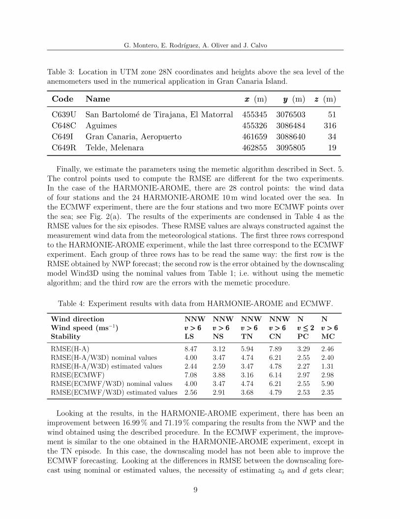
Table 3: Location in UTM zone 28N coordinates and heights above the sea level of theanemometers used in the numerical application in Gran Canaria Island.

Code Name xxx (m) yyy (m) zzz (m)

C639U San Bartolome de Tirajana, El Matorral 455345 3076503 51

C648C Aguimes 455326 3086484 316

C649I Gran Canaria, Aeropuerto 461659 3088640 34

C649R Telde, Melenara 462855 3095805 19

Finally, we estimate the parameters using the memetic algorithm described in Sect. 5.The control points used to compute the RMSE are different for the two experiments.In the case of the HARMONIE-AROME, there are 28 control points: the wind dataof four stations and the 24 HARMONIE-AROME 10 m wind located over the sea. Inthe ECMWF experiment, there are the four stations and two more ECMWF points overthe sea; see Fig. 2(a). The results of the experiments are condensed in Table 4 as theRMSE values for the six episodes. These RMSE values are always constructed against themeasurement wind data from the meteorological stations. The first three rows correspondto the HARMONIE-AROME experiment, while the last three correspond to the ECMWFexperiment. Each group of three rows has to be read the same way: the first row is theRMSE obtained by NWP forecast; the second row is the error obtained by the downscalingmodel Wind3D using the nominal values from Table 1; i.e. without using the memeticalgorithm; and the third row are the errors with the memetic procedure.

Table 4: Experiment results with data from HARMONIE-AROME and ECMWF.

Wind direction NNW NNW NNW NNW N NWind speed (ms−1) v > 6v > 6v > 6 v > 6v > 6v > 6 v > 6v > 6v > 6 v > 6v > 6v > 6 v ≤ 2v ≤ 2v ≤ 2 v > 6v > 6v > 6Stability LS NS TN CN PC MC

RMSE(H-A) 8.47 3.12 5.94 7.89 3.29 2.46RMSE(H-A/W3D) nominal values 4.00 3.47 4.74 6.21 2.55 2.40RMSE(H-A/W3D) estimated values 2.44 2.59 3.47 4.78 2.27 1.31RMSE(ECMWF) 7.08 3.88 3.16 6.14 2.97 2.98RMSE(ECMWF/W3D) nominal values 4.00 3.47 4.74 6.21 2.55 5.90RMSE(ECMWF/W3D) estimated values 2.56 2.91 3.68 4.79 2.53 2.35

Looking at the results, in the HARMONIE-AROME experiment, there has been animprovement between 16.99 % and 71.19 % comparing the results from the NWP and thewind obtained using the described procedure. In the ECMWF experiment, the improve-ment is similar to the one obtained in the HARMONIE-AROME experiment, except inthe TN episode. In this case, the downscaling model has not been able to improve theECMWF forecasting. Looking at the differences in RMSE between the downscaling fore-cast using nominal or estimated values, the necessity of estimating z0 and d gets clear;

9


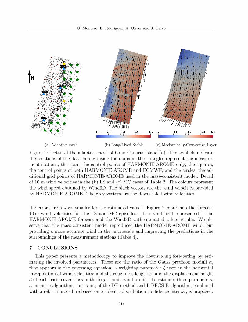
(a) Adaptive mesh (b) Long-Lived Stable (c) Mechanically-Convective Layer

Figure 2: Detail of the adaptive mesh of Gran Canaria Island (a). The symbols indicatethe locations of the data falling inside the domain: the triangles represent the measure-ment stations; the stars, the control points of HARMONIE-AROME only; the squares,the control points of both HARMONIE-AROME and ECMWF; and the circles, the ad-ditional grid points of HARMONIE-AROME used in the mass-consistent model. Detailof 10 m wind velocities in the (b) LS and (c) MC cases of Table 2. The colours representthe wind speed obtained by Wind3D. The black vectors are the wind velocities providedby HARMONIE-AROME. The grey vectors are the downscaled wind velocities.

the errors are always smaller for the estimated values. Figure 2 represents the forecast10 m wind velocities for the LS and MC episodes. The wind field represented is theHARMONIE-AROME forecast and the Wind3D with estimated values results. We ob-serve that the mass-consistent model reproduced the HARMONIE-AROME wind, butproviding a more accurate wind in the microscale and improving the predictions in thesurroundings of the measurement stations (Table 4).

7 CONCLUSIONS

This paper presents a methodology to improve the downscaling forecasting by esti-mating the involved parameters. These are the ratio of the Gauss precision moduli α,that appears in the governing equation; a weighting parameter ξ used in the horizontalinterpolation of wind velocities; and the roughness length z0 and the displacement heightd of each basic cover class in the logarithmic wind profile. To estimate these parameters,a memetic algorithm, consisting of the DE method and L-BFGS-B algorithm, combinedwith a rebirth procedure based on Student t-distribution confidence interval, is proposed.

10


A numerical experiment was carried out on a real case in Gran Canaria Island. Inthis case, the input values of the model came from two different models: HARMONIE-AROME, and ECMWF; and the control points were some measurement stations andmesoscale model nodes over the sea. Some episodes with different atmospheric conditionshave been considered. In all cases, the wind prediction of the diagnostic model with theestimated parameters was closer to the measurement data than the one provided by themesoscale model. Accordingly, we conclude that the proposed approach, combining pa-rameter estimation and a mass-consistent model, is an efficient tool for NWP downscaling.

ACKNOWLEDGEMENTS

This work has been supported by the Spanish Government, ”Secretarıa de Estado deInvestigacion, Desarrollo e Innovacion”, ”Ministerio de Economıa y Competitividad”, andFEDER, grant contract: CTM2014-55014-C3-1-R.

REFERENCES

[1] National Technique Team SIOSE, Documento Tecnico SIOSE2005 Version 2.2. Tech-nical report, D.G. Instituto Geografico Nacional, Madrid, 2011. In Spanish.

[2] Oliver, A., Rodrıguez, E., Escobar, J.M., Montero, G., Hortal, M., Calvo, J., Cascon,J.M. and Montenegro, R., Wind forecasting based on the HARMONIE model andadaptive finite elements. Pure Appl. Geophys., Vol. 172, pp. 109–120, 2015.

[3] Montero, G., Rodrıguez, E., Oliver, A., Calvo, J., Escobar, J.M. and Montenegro,R., Optimisation technique for improving wind downscaling results by estimatingroughness parameters. J. Wind Eng. Ind. Aerod., Vol. 174, pp. 411–423, 2018.

[4] Storn, R. and Price, K., Differential Evolution – A Simple and Efficient Heuristic forGlobal Optimization over Continuous Spaces. J. Glob. Optim., Vol. 11, pp. 341–359,1997.

[5] Byrd, R.H., Lu, P., Nocedal, J. and Zhu, C., A Limited Memory Algorithm for BoundConstrained Optimization. SIAM J. Sci. Comput., Vol. 16, pp. 1190–1208, 1995.

[6] Zilitinkevich, S.S., Fedorovich, E.E. and Shabalova, M.V., Numerical model of a non-steady atmospheric planetary boundary layer, based on similarity theory. Bound.-Lay. Meteorol., Vol. 59, pp. 387–411, 1992.

[7] Zilitinkevich, S.S., Johansson, P.E., Mironov, D.V. and Baklanov, A., A similarity-theory model for wind profile and resistance law in stably stratified planetary bound-ary layers. J. Wind Eng, Ind. Aerod., Vol. 74–76, pp. 209–218, 1998.

[8] Zilitinkevich, S.S., Tyuryakov, S.A., Troitskaya, Y.I. and Mareev, E.A., Theoreticalmodels of the height of the atmospheric boundary layer and turbulent entrainmentat its upper boundary. Atmospheric and Oceanic Physics, Vol. 48(1), pp. 150–160,2012.

11


[9] Andersson, E., User guide to ECMWF forecast products. Technical report, ECMWF,2015.

[10] Bengtsson, L., Andrae, U., Aspelien, T., Batrak, Y., Calvo, J., de Rooy, W., etal, The HARMONIE-AROME model configuration in the ALADIN-HIRLAM NWPsystem. Monthly Weather Review, Vol. 145(5), pp. 1919–1935, 2017.

[11] Bossard, M., Feranec, J. and Otahel, J., CORINE land cover technical guide Adden-dum 2000. Technical report, European Environment Agency; Copenhagen, 2000.

[12] National Technique Team SIOSE, Manual de Fotointerpretacin SIOSE - Version 2.Technical report, D.G. Instituto Geografico Nacional, Madrid, 2011.

[13] Taylor, P.A., Comments and further analysis on effective roughness lengths for usein numerical three-dimensional models. Bound.-Lay. Meteorol., Vol. 39, pp. 403–418,1987.

[14] Greiner, D., Emperador, J.M. and Winter, G., A Limited Memory Algorithmfor Bound Constrained Optimization. Comput. Methods Appl. Mech. Engrg., Vol.193(33–35), pp. 3711–3743, 2004.

[15] Zilitinkevich, S.S., Mammarella, I., Baklanov, A.A. and Joffre, S.M., The effectof stratification on the aerodynamic roughness length and displacement height.Bound.-Lay. Meteorol., Vol. 129, pp. 179–190, 2008.

12

Documents

PARAMETER ESTIMATION IN A DIAGNOSTIC WIND MODEL … · Grassland, Forest, Scrubs, No Vegetation, Arti cial Coverage, Wet Coverage and Water Coverage) ... PST Grasslands 0:09 0:001{0:15