Embed Size (px)
Citation preview
R E P O R T
h 00 rD -
I
pe: U
PARAMETRIC ANALYSIS OF MICROWAVE AND LASER SYSTEMS FOR COMMUNICATION AND TRACKING
Volume I1 - System Selection
Prepared by HUGHES AIRCRAFT COMPANY Culver City, Calif. 902 3 0
for Goddard Space Flight Center
N A T I O N A L A E R O N A U T I C S A N D S P A C E A D M I N I S T R A T I O N W A S H I N G T O N , D . C. FEBRUARY 1971
I
https://ntrs.nasa.gov/search.jsp?R=19710010163 2018-07-06T11:51:41+00:00Z

" TECH LIBRARY KAFB, NM
00b0807 "" . . ~ ~. - ..
1. ReDort No ... NASA CR-1687
2. Government Accession No.
-Title and Subtitle - " 1 ... .~ ~~ ~ .~ "_
Parametric Analysis of Microwave and Laser Systems for Communication and Tracking; Volume II - System Selection
~~~~ .. - - ~ ~ . . . . ~
7. Author(s) "~ ...
9. Performing Orgonization Nome and Address " .~~ ~ . ~ . . .. . ~ - ".
Hughes Aircraft Company Culver City, California
~~ ~ _ _ _ ~ 2. Sponsoring Agency Name and Address
National Aeronautics and Space Administration IPJa'shingkon, D . C . 20546
5. Supplementory Notes Prepared iico&ieTa%= al l the avai labl&
"" - 3. Recipient's Cotolog No.
X R G o r t D o t e
February 1971 6 . Performing Orgonizotion Code
" ~ ~
8. Performing Organization Report No
- ~- 10. Work Unit No.
11. Contract or Grant No. NAS 5-9637
--- 13. Type of Report and Period Covered
Contractor Report
14. Sponsoring Agency Code
Kperts at the Hughes Alrcratt :. L. Brinkman. the Associate Compony and edited jointly by L. S.' Stokes, the Program Manager, K
e:
Program Manager, and Dr. F. Kalil, the NASA-GSFC Technical Monitor, with L. S..Stokes being the primary contributing editor.
- ." - ~- 6 . Abstroct
" - ~ ""
Present and future space programs ore requiring progressively higher communication rates. For instance, the Earth Resources Technology Satellite-A requires about 70 MHz total bondwidth in its S-Band downlink spectra, and it appears likely that future earth observation satellites will require
hand, the frequency bands allocated via international agreements for space use are limited, and henc' more bandwidth because of the lorger number of sensors and higher sensor resolutions. On the other
the r-f spectrum is becoming crowded. However, the advent of the C-W laser system s offered a"new and wide electromagnetic spectrum for use in space telecommunications. Although the laser systems offered this "new" capability, their technological development was also new. Therefore, this study was undertaken to make a comparative analysis of microwave and laser s ace telecommunication sys terns. A fundamental objective of the study was to provide the mission pfanner and designer with reference data (weight, volume, reliability, and costs), supplementary material, and a trade-off methodology for selecting the system (microwave or optical) whi ch best suits his requirements. Thi: report is the final report of that study. Because of the large amount of material, the report is pre- sented in four volumes. This volume, Volume II, "Systems Selection," contains two major parts,
constraints, histor and plans. It is given as a foundation for understanding space communication Mission Analysis and Methodology" and "System Theory." The first part is o review of mission
goals. The methocrology or design criteria developed under this contract is also described in this
determine deep space communications l ink performance. Special treatment i s given to the determi- part and in pertinent appendices. "System Theory" describes the constraining equations used to
nation of signal to noise ratios in optical communications systems.
.'
I. Key Words (Selected by Author(s)) ".
Mission Analysis Optimum Communication Design Optical Detection Theory Optical Modulation Theory
Unclassif ied - Unlimited


PARAMETRIC ANALYSIS OF MICROWAVE AND LASER SYSTEMS FOR COMMUNICATION AND TRACKING
VOLUME I SUMMARY
VOLUME I I SYSTEM SELECTION
VOLUME I1 I REFERENCE DATA FOR ADVANCED SPACE COMMUNICATION AND TRACKING SYSTEMS
VOLUME IV OPERATIONAL ENVIRONMENT AND SYSTEM IMPLEMENTATION


ACKNOWLEDGEMENT
"Miss ion Analys is and Methodology" was l a rge ly p repared by
M r . James R. Sul l ivan and Dr . William K. Pra t t . "Sys tems Theory"
w a s l a r g e l y p r e p a r e d b y D r . P r a t t . M r . S u l l i v a n , f o r m e r l y of Hughes
Ai rc ra f t Company is c u r r e n t l y w i t h S y s t e m s A s s o c i a t e s . D r . P r a t t ,
f o rmer ly a t Hughes A i rc ra f t Company , is p r e s e n t l y A s s o c i a t e P r o f e s s o r
of Electr ical Eng. ineer ing a t the Universi ty of Southern Cal i fornia .
V


r-
BRIEF INDEX O F VOLUME I1
P A R T 1 MISSION ANALYSIS .AND METHODOLOGY
Sect ion Page
Analys is of Poten t i a l Mis s ion Ob jec t ives . . . . . . . . . . . . . . . 8
Analys is of Miss ion Requ i remen t s . . . . . . . . . . . . . . . . . . . 32
Methodology for Optimizing Communicat ion Systems . . . . . . . 50
Methodology Examples and Conclusions . . . . . . . . . . . . . . . . 73
PART 2 SYSTEM THEORY
Optical Detect ion Noise Analysis . . . . . . . . . . . . . . . . . . . . 94
Optical Detect ion . . . . . . . . . . . . . . . . . . . . . . . . . . . . . . . 110
Modulation Methods . . . . . . . . . . . . . . . . . . . . . . . . . . . . . 136
Communicat ion Coding . . . . . . . . . . . . . . . . . . . . . . . . . . . 164
Telemet ry Communica t ions . . . . . . . . . . . . . . . . . . . . . . . . 170
Appendices
Appendix A . Communica t ion Sys tems Opt imiza t ion Methodology . . . . . . . . . . . . . . . . . . . . . . . . . A- 1
Appendix B . COPTRAN . . . . . . . . . . . . . . . . . . . . . . . . . . B- 1
v i i

DETAILED INDEX O F VOLUME I1
P A R T 1 MISSION ANALYSIS AND METHODOLOGY
P a g e
Introduction . . . . . . . . . . . . . . . . . . . . . . . . . . . . . 2 S u m m a r y . . . . . . . . . . . . . . . . . . . . . . . . . . . . . . . 4
Analys is of Poten t ia l Miss ion Objec t ives . . . . . . . . . . . . . 8
The So la r Sys t em . . . . . . . . . . . . . . . . . . . . . . . . . 8 C u r r e n t U n m a n n e d P r o g r a m s . . . . . . . . . . . . . . . . . . 10 Deep Space Miss ions . . . . . . . . . . . . . . . . . . . . . . . 16
Deep Space Probe Ins t rumenta t ion . . . . . . . . . . . . . . 20 P l a n e t a r y F l y - B y a n d O r b i t e r M i s s i o n O b j e c t i v e s . . . . . 2 2 P lane ta ry F ly -By and Orb i t e r In s t rumen ta t ion . . . . . . 24 Entry Miss ion Objec t ives and Ins t rumenta t ion . . . . . . . 26 Manned Missions . . . . . . . . . . . . . . . . . . . . . . . . . . 28
Analys is of Miss ion Requi rem.ents . . . . . . . . . . . . . . . . . 32
D a t a T r a n s m i s s i o n R e q u i r e m e n t s . . . . . . . . . . . . . . . 32 Acqu i s i t i on and T rack ing Requ i remen t s . . . . . . . . . . . 36 Communicat ion Range . . . . . . . . . . . . . . . . . . . . . . . 38 Miss ion Dura t ion . . . . . . . . . . . . . . . . . . . . . . . . . . 40 Communica t ion Sys tem Weight Res t r ic t ions . . . . . . . . 44 Miss ion Oppor tuni t ies . . . . . . . . . . . . . . . . . . . . . . . 46
The Pu rpose fo r a Communicat ions Methodology . . . . . 50 Major Sys tem Parameters Used in the Methodology . . . 52 Types of System Classified in the Methodology . . . . . . 54
Methodology . . . . . . . . . . . . . . . . . . . . . . . . . . . . 56 S t ruc tu ra l De ta i l of Methodology Implementat ion . . . . . 58 S y s t e m B u r d e n P a r a m e t e r s . . . . . . . . . . . . . . . . . . . 62 Bas i s fo r P re sen t Burden Re la t ions and Cons tan t s . . . . 66 U n c e r t a i n t i e s i n P r e s e n t B u r d e n R e l a t i o n s . . . . . . . . . 70
Methodology Examples and Conclusions . . . . . . . . . . . . . . 74
Feas ib i l i t y of Lase r s fo r Space Communica t ions . . . . . 76
Microwave) to Miss ion . . . . . . . . . . . . . . . . . . . . . 78
Des ign Cr i t e r i a . . . . . . . . . . . . . . . . . . . . . . . . . . 8 2
Deep Space Probe Objec t ives . . . . . . . . . . . . . . . . . . 18
Methodology for Optimizing Communicat ion Systems . . . . . 50
Keys tone Op t imiza t ion P rocedures Used i n t he
Implementa t ion of Des ign Cr i t e r i a i n a U s e a b l e F o r m . . 74
Capabili ty of C o m m u n i c a t i o n S y s t e m ( L a s e r o r
Mic rowave and Lase r Sys t ems Compared Us ing
ix

&-J ~ .
. . DETAILED INDEX OF VOLUME I1 (Continued)
PART 2 SYSTEM THEORY
P a g e
Introduct ion . . . . . . . . . . . . . . . . . . . . . . . . . . . . . 90 S u m m a r y . . . . . . . . . . . . . . . . . . . . . . . . . . . . . . . 92
Opt ica l Detec t ion Noise Analys is . . . . . . . . . . . . . . . . . . . 94
Opt ica l Detec t ion Methods . . . . . . . . . . . . . . . . . . . . 94 T h e r m a l N o i s e . . . . . . . . . . . . . . . . . . . . . . . . . . . . 98 F l i c k e r N o i s e . C u r r e n t N o i s e . a n d D a r k - C u r r e n t
Shot Noise . . . . . . . . . . . . . . . . . . . . . . . . . . . . . 100 Photon Fluctuat ion. Shot . and Generat ion -
Recombina t ion Noise . . . . . . . . . . . . . . . . . . . . . . 102 Background Radia t ion Noise . Radia t ion F luc tua t ion
Noise. and Phase N0is .e . . . . . . . . . . . . . . . . . . . . . 106 Optical Detect ion Noise . . . . . . . . . . . . . . . . . . . . . . 108
Optical Detect ion . . . . . . . . . . . . . . . . . . . . . . . . . . . . . 110
Opt ica l Detec t ion S ta t i s t ics . . . . . . . . . . . . . . . . . . . 110 Opt ica l Di rec t Detec t ion . . . . . . . . . . . . . . . . . . . . . 116 Opt ica l Heterodyne Detec t ion . . . . . . . . . . . . . . . . . . 122 Optical Homodyne Detection . . . . . . . . . . . . . . . . . . . 130
Modulation Methods . . . . . . . . . . . . . . . . . . . . . . . . . . . 136
Introduction . . . . . . . . . . . . . . . . . . . . . . . . . . . . . 136 Type I Modulat ion Systems . . . . . . . . . . . . . . . . . . . 138 Type I1 Modula t ion Sys tems . . . . . . . . . . . . . . . . . . . 140 Type I11 Modula t ion Sys tems . . . . . . . . . . . . . . . . . . 142 Optical Pulse Code Intensi ty Modulat ion . . . . . . . . . . . 146 Optical PCM Polar izat ion Modulat ion . . . . . . . . . . . . 148 Opt ica l PCM Frequency Modula t ion . . . . . . . . . . . . . . 152 Opt ica l PPM In tens i ty Modula t ion . . . . . . . . . . . . . . . 154 Radio Ampl i tude . Frequency . and Pulse Code
Modulation . . . . . . . . . . . . . . . . . . . . . . . . . . . . . 156 Pseudo Random Noise Modulat ion for Radio
Communica t ions Sys t ems . . . . . . . . . . . . . . . . . . . 160
Communication Coding . . . . . . . . . . . . . . . . . . . . . . . . . 164 Da ta Compress ion . . . . . . . . . . . . . . . . . . . . . . . . . 164 Synchroniza t ion . . . . . . . . . . . . . . . . . . . . . . . . . . . 168
Te leme t ry Communica t ions . . . . . . . . . . . . . . . . . . . . . . 170
FM and FM/FM L ink Equa t ions . . . . . . . . . . . . . . . . 170 Degrada t ion Caused by Nonidea l Pos tde tec t ion
F i l t e r ing . . . . . . . . . . . . . . . . . . . . . . . . . . . . . . 174
X

PART 1 MISSION ANALYSIS AND METHODOLOGY
Page Introduction . . . . . . . . . . . . . . . . . . . . . . . . . . . . . . . . . . . . . . . . . . . . . . . . . . . . . . . 2
Summary . . . . . . . . . . . . . . . . . . . . . . . . . . . . . . . . . . . . . . . . . . . . . . . . . . . . . . . . . 4
Analysis of Potential Mission Objectives . . . . . . . . . . . . . . . . . . . . . . . . . . . . . . . . . . . . . . . . 8
Analysis of Mission Requirements . . . . . . . . . . . . . . . . . . . . . . . . . . . . . . . . . . . . . . . . . . . 3 2
Methodology for Optimizing Communication Systems . . . . . . . . . . . . . . . . . . . . . . . . . . . . . . . . 50
Methodology Examples and Conclusions . . . . . . . . . . . . . . . . . . . . . . . . . . . . . . . . . . . . . . . 74
1

:+* Mission Analjrsis and Methodology ~ ,3 f p
&fg h,
INTRODUCTION
The purpose and topics of this par.t are introduced.
Mission analysis and methodology is divided into four sections. A brief description of each section and the topies they contain is given below.
An Analvsis of Potential Mission Obiectives
Clearly it is necessary to determine the type of space mission, the data requirements and time duration before a communication system can be designed. This section contains general background data on the solar system and on the type of manned and unmanned missions currently being planned. From this data typical payload and data rates are derived.
Analysis of Mission Requirements
Once a particular mission is selected, several design constraints are imposed upon the communication system. Those discussed in this sec- tion include constraints of data rate, acquisition and tracking, comrnuni- cation range, mission duration and communication system weight res t r ic t ions.
Methodoloery for Optimized Communication Systems
A goal of this study was to provide a means of impartially describing the optimum communication system for a particular mission. A method- ology is given as are computer derived results. The methodology designs the least expensive or lightest communications system within the con- s t ra in ts of the range equation.
Methodoloev Examdes and Conclusions
Computer results of the methodology are given which compare laser and microwave systems for a Mars mission.
2


Mssion Analysis and Methodology
SUMMARY
Mission goals have been documented and optimum communication analysis methods have been developed. Sample communication problems are given to illustrate optimum configurations.
The mission analysis documents potential missions and provides a com- munication methodology which allows the selection of the best communi- cation implementation for a given mission.
Missions
In general , deep space missions can be divided into four classes: 1) deep space probes which simply pass through interplanetary space making scientific measurements of the space environment encountered, 2) f ly- by missions which have as their objectives a specific planet, but which make scientific measurements of that planet only during the fly-by phase, 3) planetary orbiter missions in which the spacecraft is placed into orbit about the target planet, and 4) planetary entry and lander missions in which the spacecraft or capsule enters the planetary atmosphere and t ransmits data e i ther direct ly back to Earth or re lays i t through the spacecraft bus back to Earth.
Mission and TvDe of Communication Svstem
When the general capabilities of laser and microwave systems are com- pared with the Data Rate Estimates, certain conclusions may be reached, these are noted below.
a A radio communication system should be used for space probes operating at planetary distances. This is largely due to the low data rate which may easily be accommodated by existing radio systems,
0 An optical communication system should be used for a planetary orbit ing mission. This is due to the very large amount of data which may be gathered using imagery sensors at these long ranges and which will be gathered at high rates for extended periods of t ime. Thus, not offering an opportunity to store the data and transmitting it at a s lower ra te .
a An optical communication link is also appropriate for manned lander mission. Here the high data rate obtained from imagery sensors l eads to the selection of optical communications.
a In flyby missions the data rate can be high for a short period of time. This allows the use of a storage and playback mode and a radio link. The radio link would also be necessary s ince, with a flyby mission, continuous communication coverage is usually required during the critical flyby time. This could not be obtained with an optical system unless the additional com- plexity of an earth orbit ing optical receiving station is used to prevent blockage by clouds.
4

0 F o r a manned orbiting mission a radio system is likely best even though high, long te rm da ta ra tes may be expec ted . The reason for this is the additional difficulty in decoupling man caused mechanical disturbances which are difficult and expen- s ive ( in terms of control system fuel (weight) to decouple from the optical pointing system.
An optical communication system can provide high data rates at planetary distances. Due to the specialized care required in pointing and tracking, this high data rate transmission becomes the principle features of l a se r communications. However this is not the only type of communication required by a spacecraft . In fact , there is generally a requirement for continual telemetry data which allows the earth st,ations to monitor the spacecraft performance and to determine the spacecraft 's posit ion. In addition to the t ransmission of telemetry data, the spacecraft must receive commands and beacon signals from earth. The two functions, commands and telemetry, are accomplished best , by far, with a radio system. Thus i t is seen that any optical system is real ly a combination of laser/optical and microwave, with the microwave being a relatively low performance communication system (and thus much less costly and lighter than a link that transmits the high data gates) and the optical sys- t e m being designed to transmit the high data rates.
5


MISSION ANALYSIS AND METHODOLOGY
Analysis of Potential Mission Objectives
CURRENT PROGRAMS
Page The Solar System . . . . . . . . . . . . . . . . . . . . . . . . . . . . . . . . . . . . . . . . . . . . . . . . . . . . . 8
Current Unmanned Programs . . . . . . . . . . . . . . . . . . . . . . . . . . . . . . . . . . . . . . . . . . . . . . 10
Deep Space Missions . . . . . . . . . . . . . . . . . . . . . . . . . . . . . . . . . . . . . . . . . . . . . . . . . . . 16
Deep Space Probe Objectives . . . . . . . . . . . . . . . . . . . . . . . . . . . . . . . . . . . . . . . . . . . . . . 18
Deep Space Probe Instrumentation . . . . . . . . . . . . . . . . . . . . . . . . . . . . . . . . . . . . . . . . . . 2 0
Planetary Fly-By and Orbiter Mission Objectives . . . . . . . . . . . . . . . . . . . . . . . . . . . . . . . . . . . 22
Planetary Fly-By and Orbiter Instrumentation . . . . . . . . . . . . . . . . . . . . . . . . . . . . . . . . . . . . 24
Entry Mission Objectives and Instrumentation . . . . . . . . . . . . . . . . . . . . . . . . . . . . . . . . . . . . 26
Manned Missions . . . . . . . . . . . . . . . . . . . . . . . . . . . . . . . . . . . . . . . . . . . . . . . . . . . . . 2 8

, . Mission Analysis and Methodology Analysis of Potential Mission Objectives
' I
THE SOLAR SYSTEM
examination of the major bodies in the solar system helps guide the selection of preferred deep space missions, and associated telecommunications requirements. The best way to fulfill these requirements is the theme of this report .
- ~~ " ~~ ~. ~ ~~. ~ - ~~ "" ~~ "
The choice of a space communication system for a par t icular mission must take into account
1. Probable objectives of the mission under consideration
2. Reflection of these mission objectives into communication system requirements.
This involves definition of communication range, system lifetime requirements, and total data goals. These in turn affect data trans- mission rate and data processing and storage facil i ty requirements. The composite mission constraints must then be reconciled with the restrictions on communication system such as weight, volume and power which are imposed by technological limitations. It is the purpose of this Mission Analysis Section to present: 1) potential mission objectives, 2 ) the conditions of these missions which are pertinent to communications, and 3 ) the demands which these missions will impose on a communications system.
The solar system consists of the sun as center body and a great number of smaller bodies revolving about the sun with the solar mass represent- ing about 99. 2 percent of the total mass of the solar system.
The extrasolar matter can be divided into the following groups:
1. Planets and their satell i tes (see Table A)
2. Minor planets (asteroids or planetoids)
I
3. Comets
4. Meteors and dust
5. Interplanetary gas
Aside from the sun, the presently known solar system consists of nine planets, more than 1500 catalogued asteroids, 31 satell i tes, and an unknown, but very large number of comets and meteors. The mean density of interplanetary dust in the vicinity of the earth cannot be estimated presently with greater accuracy than a factor of 1000. Inter- planetary gas consisting mainly of ionized hydrogen, helium and elec- trons is thinly distributed throughout the solar system.
Al l planets of the solar system revolve about the sun in the same direction as the earth (counter-clockwise i f seen from a point above the North Pole of the earth 's orbital plane, the ecliptic plane). With
'Miluschewa, Sima, "The Solar System Environment, " IEEE Transac- tions on Aerosapce and Electronic Systems, p. 758, September 1967.
a

the exception of Pluto and Mercury, the outermost and innermost planets known, all planets move very nearly in the plane of the ecliptic, that is in the earth's orbital plane (see Figure A).2 These two facts make full utilization of the planets' orbital velocities for cotangential interplane- tary transfer orbits possible.
The main factor in determining the motion of planets, asteroids, comets and meteors is the powerful gravitational field of the sun. Planetary distances extend by a factor of 100 into space, from Mercury to ,Pluto. Some comet orbits extend considerably beyond Pluto while most aster- oidal orbits extend to 2. 8 A. U.
Table A. Physical Characteristics of the Planets
2. 42 6. IO M a s s ( ~ n c l u d r , ~ g s e I e l l l l e s ) (e = I ) 0.054b 0.81498 I 01230 0. IO77 317.89 95 12 I 4 5L 17. o.a+o. I Equolor!al sur face g r a v i l y ( e = I ) 0.380 0.893 1 . 00 0. 377 2. 54 I Ob 1.07 1.4 0.7
6. 37n 3 . 4 1 70. 4 6. 04 2. 35 2. 23 7.
o 387 0.723 I 00 I . 52
Aphcllon drsrance (AU) 0.467 0.728 1.017 1 b6.3 5.455 10.07 20.09 30. 32 49. 34 O r h l l a l ecccn lr i c t ly ( O X I O - ~ ) 2Ob 6.79 16.73 93. 3 hiran o r h l l a l v e l v c l l v le 11 1.607 1.17b 1.00 0 . no7 n 4 7 s 11 3 7 ~ n > m n 1 x 2 n I ~ O
48.5 SI. 6 44. 31 7. 34 248. I 1
k m l s . .
47.90 3 5 . 0 5 29 77 L4.02 1 3 . 0 5 9.64 6.797 5.43 4.73 42.82 31 60 22. 30 1 7 . 8 0 1 5 . 6 103 [ ( I s 157 I9 114 9 6 97. 70 73 81
. ." . ". .. ."_ " ._, Prrtod "1 rcvOll l l io" ( D i I ) 0. 2 4 1 0.611 1.00 1 83 1 1 . 8 6 29.46 84.0 l b 4 . 8 247.1
""_ SATELLITE IN DIRECT ORBIT SATELLITE IN RETROGRADE ORBIT
MERCURY 4 JUPITER
0 VENUS h SATURN Q EARTH URANUS d M A R S NEPTUNE
OUTER SATELLITE SYSTEM
INNER SATELLITE SYSTEM
I I I I I l l 1 I I I I 1 1 1 1 I I I I I l l 1
0.3 1 IO 1 0 0
DISTANCE FROM SUN, A.U.
Figure A. Orbital Inclinations of Planets and Their Satellites in the Solar System
'Serfert, H. S . , Space Technology, John Wiley and Sons, New York, 1959.
9

Mission Analysis and Methodology Analysis of Potential Mission Objectives
CURRENT UNMANNED PROGRAMS
Mission Goals, Status (as of January 1969), and Contractors are given for 29 cur ren t unmanned probes.
A variety of lunar and planetary missions are currently planned or under active consideration by NASA. Unmanned interplanetary missions under considerat ion are summarized in Table A.
In 1969 a double fly-by mission to Mars is planned with an advanced vers ion of the successful Mariner IV spacecraft . With these flights additional photographic coverage will be obtained and more detailed observations of the Martian atmosphere will be made preliminary to the subsequently planned Voyager mission in 1973. A comparison between the Mariner I V spacecraft and the proposed 1969 Mariner-Mars space- craf t is shown in Table B. Proposed experiments include IR, UV, and television scanning for atmosphere and planetary surface observations as well as measurements of interplanetary f ields and particles.
The Voyager Program is directed initially toward the exploration of Mars and is geared to first flights during the 1973 opportunity. How- ever, the Voyager, as a basic spacecraft system, is l ikely to serve as a vehicle for more detailed exploration of Venus and Jupiter. The cur- rent Voyager concept consists of three basic modules. The f irst is the spacecraft bus, houses the necessary electronics, at t i tude control, and communications systems for interplanetary and orbital operations as well as necessary support for the landing capsule. Second, a propulsion system which provides the necessary propulsion for midcourse correc- tion and orbital insertion and thirdly the landing capsule. Preliminary Voyager spacecraf t system designs are summarized in Table C.
'Space/Aeronautics, January 1969.
10
MARINER MAR: , . ~ " :
PIONEER
-
. .. - 'SURVEYOR
"
MARINER VENUS
PLANETARY EXPLORER
AIR DENSITY, INJUN
..
lSlS ( INTERNATIONAI SATELLITE FOR
STUDIES) IONOSPHERIC
Table A. U. S . Unmanned Space Science Projects
Mlarlonr, 1.chnk.l Goah I Shlur, Mllmrtann Fundlng, Conlmcton
PLANETARY AND LUNAR VEHICLES
Marlner Man '(x: far llybys for atmoapherlc studles. Marlner M a n O W ; nsar flybys lor closer examlnatlon of lonospherlc and at- mospherlc chsracterlstlcs, shape of planst. Mariner Mars '71: to orbit planet. conduct topographlcal end thermal mapplng, study atmospherlc dynsmlc8. seasonal anvlron- menlal varlatlona. Marlner Tlten Mars '73: orbiter and soft-lander to study surlece. blosphsrlc. and entry characterlstlcs. Mar- iner Mare '75-'7?: large surface lab wlth re- turn module to brlng back a011 samplas. Boosters: MM '(x, Atlas-Agena; MM '69 and 71. Atlas-Centaur; MTM '73. Tltan 3D-Can-
taur; MM '75-77. Saturn 5 or Saturn 5-Nerva.
Langley. MM ' 7 5 - 7 : NASA-OSSA. MM'~, '69 . '71:NASAJPL.MTM'73:NASA-
Solar-orbltlng probes of very high mag-
Ira and dlstrlbutlon 01 partlcles and flelds netlc cleanllness lor study of energy spac-
durlng 11-yr solar cycle. Flrat verslons or- blted 0.61.2 AU from sun: exlended ver- slon, 0.46.6 AU: advanced veralon. 0.26.3 AU. Boosters: TAD, Atlas-Centaur-TEl4 (Pioneers F, G). NASA-Ames.
Solt lunar landing 01 unmannod Instrumen- ted spacecraft with tv camera, touchdown straln gage Instrumenlation. Surveyor 3. 4 carried surface sampler; 5. 6 conducted alpha backscalter analysls of lunar sur- lace; 7 carrled sample and backscaner analysls experlments. Booster: Double-burn Centaur. NASA-JPL.
Mariner Venus '67: lar llyby lor prellmlnary atmospherlc studles wlth modlfled Marlner
atmospherlc probes. Mariner Multlprobe Mars. Marlnor Venus '73-'75: near flyby 01
Buoyant Statlons: balloons in Vonuslnn or- bit. to launch probes for atmospherlc stud- !es. Boosters: MV '67. Atlas-Agene; MV '73-
NASAJPL: MV '73-75. Multlprobe: NASA- 75. Multlprobe. Atlas-Centaur. MV '67:
OSSA.
LOW-cost. long-llfe Explorer-type craft (modlfled Imp deslgn) for study of plane- tary envlronments; to orblt Mars In '73, '75. 'T I ; Venus In '72. '73. '75. ' T I ; Mercury In ' 73 . Booster: TAT-Delta, NASA-Goddard.
NEAR-EARTH STUDY
Two jolntly-launched sa1e1111es. Alr Denslty craft Is 12-ft Inflatable sphere slmllerto Ex-
changes In upper atmosphere. Injun meas- plorer 9. 19. 24; measures elr denslty
mosphere, low-lroquency lonospherlc radio ures downflux 01 redletlon upon upper at-
emlsslons. Booster: Scout. NASA-OSSA, Langley.
Jolnt prolect of NASA and Canadlan De- lense Research Board to study Ionosphere throughout solar cycle. Canadlan Alouette swept-frequency topslde sounder, US. lon- osphere Explorer fixed-lrequency sounder. US. Dlrect Measurement Explorer meas- ures electron and Ion dendty. tempera- ture. Boosters: Thor-Agena (early lala). Delta (Isls A-C). NASA-Goddard.
-
= - " ." . . ~ -~ . .
"" - .. . - ~ ~~
~.
MM '(x st111 reepondlng to demand for slg- nals from aoler orbit. Two MM 'W antel- lites and expsrlmenta undsr test; mlsslons scheduled for Feb. end Apr. '8. MM '71 mlsslon approved by NASA; experlment aa-
aprlng and 1811 '71. MTM '73 (Vlklng) ep- Iactlon underway; flights achsdulsd lor
proved an llns Item for FV '70 budget; Iand- Ing almulatlon late 'W; two '73 IIlghta planned. MM '75-77 undsr atudy.
PJoneer 6 launched '65 to 0.014 AU 01 sun.
01 1.13 AU aphellon. 1 AU perlhellon. Pio- Ploneer 7 launched '88; lags earth In orblt
neer 6 flew Dec. '67; Ploneer B on Nov. 15. '88. Ploneer E, F. G scheduled for '68. '72.
old belts. '73: F end G mny study Juplter and aater-
~
Surveyor 1 soft-landed June '€6: Surveyor 2 Impacted Sep. '€6 In out-of-control tum-
Jan. 9. '68. ble; Surveyors 3, 5. 6 landed In '67, 7 on
MV '67 stlll respondlng to demand for slg- nals. MV '73-'75 mlsslon epproved as line Item for FY '70 budget. Prellmlnary deslgns 01 buoyant statlons In '68; two planned but not approved lor '75.
~~
Prellmlnary design work underway at God- dard by Imp project team.
AD launches In '61 and '(x. Flmt ADll
plorer 38, a) In Aug. '88. launch (Explorer 24, 25) In '(x. second (Ex-
Alouene 1 launched '62; Ionosphere Ex- plorer 20, 'M;Alouette 2, '65. lsls A planned for Jan. 22, '69 launch Into low-altitude,
C lor '71. nearly polar orblt. 181s 8 scheduled lor *m,
All Marlnor prolects through FY
and '71. Wm; MM '73, tom; ed- '88, .It. t250m. FY '80: MM '8
vanced mlsslons. Wm.
Through FY '88. $70m; FY 'a. Om (excludlng launch vehlcles). TRW Systems (prlme).
Through FY '67. Wl3m; FY '69,
c ra l t ) . $ 1 0 3 . 3 ~ 1 (boosters). tlm. Est. total: W . 9 m (space-
Hughes (prlme).
(above). Marlln Marletla (prellm- Fundlng: see Marlner Mars
lnarydeslgnofbuoyantstatlons).
Funded as pnrt of Imp (see below).
Through FY '88. Om; FY 'M. 10.7m. Est. total: U.6m (space- craft). U.4m (boostere). Injun:
(spacecraft assembly). Iowa State (prlme); Bendlx
Through FY ' 8 8 . S4m; FY 'a, $25.6m plus *il.am lor boosters. S1.4m. Est. totel lor 11 lala:
11

Mission Analysis and Methodology Analysis of Potential Mission Objectives
CURRENT UNMANNED PROGRAMS
Table A. U. S. Unmanned Space Science Projects (Continued)
I 1 T i I
1
Explorer 1.9 launched '63; Explorer 21 ('64) had parlgee of only W,Mo mi (uppar-stage fallure). Flrat Lunar Imp (D. Explorer a) falled to achleva planned lunar orblt In '0
*WI.MO-km earth orbit. Imp E (Explorer 35) (perturbed 2nd-atage flrlng). want Into
Into lunar orblt and Imp F (Explorer 34) Into
for ' 6 9 earth orblt wlth 128.Mo-ml apogee; elllptlcal earth orblt In 37. Imp G planned
Imp I, H. J approved for '70, '71. '72.
Through FY 'W, S u m : Fy '69. S7m. Eat. totals: Wlm (IO apace- craft). S33.3m (booaters). In- house program.
Study of radlatlon environment of clslunar space throughout a solar cycle. a8 wall as
earth's magnstoaphere; development of 01 Intarplanetary magnetlc flelds and
solar-flare predlctlon method; amessmant of radlatlon hazard for Apollo. Satellltes earth-anchored (135 Ib) or lunar-anchored (I81 Ib). Booster: TAD. NASA-Qoddard.
1 BIOSATELLITE Study of blologlcal system responses to effects of welghtlessness. radlatlon, lack of earth's perlodlclty. Experlmenls at cellu-
almed at study of embryologlcel develop- lar. tlssue. organ. and organlam levels
ment. growth. and physlologlcal functlons In organlsms such as primates. Three mls- slons requlred to accommodate payloads. Booster: TAD. NASA-Ames.
Through FY '68, Slam: FY '69, SZIm. Est. totals: S138.5m (6 sat- ellltas). (21.5m (boosters).
fellure (capsule was no: recovered). Blosat Biosatellite 1 launched Dec. '66: sclentlflc
? made successful but shortened fllght In 67. Blosat D and backup Blosal F to carry prlmatea on =day fllghts In '89, '70. Blo- sals C and E for n-day lllghts canceled Dec. '68. Studles belng conslderad for follow-on Blosat. lmprovsd Blosat. Blopl- oneer. manned orbltlng blotechnology la- boratories (010 A-F), Advanced Blosat.
Two Identical Owl satelllles to be launched 1 month apart In '70 or earller.
- (prime). FY '69. $7m, total: S9m. Rice U. Owl Explorers to study near-earth atmOS-
glow) as they correlate wlth trapped radle- pherlc phenomena (e& aurora end alr-
tion belts and preclpllated radlatlon. Sat- ellltes deslgned for unlverslty use. Boost- ar: Scout. NASA-Wallops.
To provide group of experlmenters wlth opportunltles to fly slngle or dual sensors for synoptlc and related studles; may be
NASA-Goddard. launched I n cIu6ters. Booster: Scout.
EXPLORER
"
FSS-A scheduled for launch In '70, -B In 71.
-
I SATELLITE SMALL SCIENTIFIC
FY '69, t2m. In-house program.
OBSERVATORIES
Study of spectral raglons lnvlslble from earth becarlae of atmospherlc abaorptlon.
OAO carrlea loa, Ib of Inatrumenta. welgha In 35-deg-lncllned clrcular orblt at 500 ml.
4aW Ib. Llmltad payload available for aec- ondary mlsslons. Booster: Atlas-Centaur. NASA-Qoddard.
. Through FY '€8, SSZm: FY '6% S n m . Est. total: SUOm (space- craft). S107m (boosters). Grum- man (prlme). GE-MSD (stabll- Izatlon and control). Kollaman Instruments (star trackers). Wastlnghousa Research Lab (tv).
OAO-AI. launched '5% suffered power fall- ure on second day. rendered no data. OAO- 1 launched successfully Dec. 7. 'BB. OAO-B and -C scheduled for '69 and '70.
ORBITING ASTRONOMICAL OBSERVATORY
ASTRONOMY RADIO
EXPLORER
RAE-A (Explorer 38) launched Jul. '68 Into 3700-ml circular orbit wlth 58 deg retro- grade Incllnatlon; each of four 750-ft an- tenna booms successfully extended. RAE-B scheduled for '69 to complete mapping of radio source8 In sky.
Through FY '€8, W m ; FY 'Ea, Sl.5m. Total: S46m for in-house program.
Measurements of frequency. Intensity. dl- rectlon of radlo signals from celestlal sources In 0.250.2-MHz range. Mapplng of radlo sources on all-sky bash wlth two satellites. Bwstbr: TAD. NASA-Goddard.
tary and solar sources on all-sky basis from Detect x-rays and gamma rays from plane-
%mi orblt wlth 30-deg Incllnatlon to ecIIpIIc. Booster: Delta. NASA-Qoddard.
to study solar phenomena from outalde &bllized apace. platforms In earth orblt
distorting elfacts of atmosphere through 11-year solar cycle. Fan-shaped atablllzed aectlon connects to rotetlng wheel contaln- Inp Instruments. Booster:Thor-Delta. NASA- Goddard.
SAS-A (x-ray) belng bullt for launch In '70, SAS-B (gamma ray) for '71.
plus Sl.5m per booster. N '83. Sm. Amerlcen Science a Engl- neerlng (SAS-A x-ray experl- ment. S . 4 m ) .
Through N '67. $7lm: FY '69. t12m. Eat. total: a m (space- craft). S25m (booatera). Bal l Bros. (prime).
SATELLITE
0 8 0 1 ('62) collected hr of data: Os0 2 ('a) made 41W orblts In B months; 0 8 0 C ('65) lost due to launch vehlcle fnilure; Ow 3, 4 launched '67. 080 F and Q planned for '69. H for '70.
Through FY 'W. W3n-k '69.- S13m. Est. total: $ZIB.lm (space-
Systems (prlma). Ogo 5: Amerl- craft). U7.lm (boosters). TRW
nara). Hoffman Elactronlca can Standard (horlzon scan-
aolar cel ls). L ORBITING GEOPHYSICAL OBSERVATORY
Ego 1 launchad '64, st111 operatlng Inter- mittently. Ego 3 ('66) performed for sched- uled 4.3 days. Ogo 4 lmmehed '67: Oflo 5
Series of 3-axls-stabillzed spacecraft to study psrtlcle actlvlty. surore and slr-glow. geomagnetlc flelds. upper atmosphere composltlon. lonlzlng and heatlng energy sourcss. Orblts: hlghly eccentrlc (Ego) and polar clrcular (Pogo). Bwnters: Ego. At- las-Agana; Pogo, TAT. NASA-Qoddard.
(Ego), Mar. '68. 090 for early '69.
12
.. . .. .

. ."
Table A. U. S. Unmanned Space Science Projects (Continued)
ATS
TECHNOLOGY (APPLICATIONS
SATELLITE)
ATS
TECHNOLOGY (APPLICATIONS
SATELLITE)
NAVIGATION SATELLITE
1 "
INTELSAT 3
ESSA
SURVEY (ENVIRONMENTAL
SATELLITE)
- I
ADVANCED ASSA
"
PILOT DOMESTIC COMSAT
"
INTELSAT 4
SERWCE SATELLITES
Y l u k n a , Tochnlcal Goala
Satellites l o develop cloud surdelllance. communlcmtlon8. stsblllzatlon, and navlga- tlon technology In synchronous orblt. Sev-
Welghls: KC-lm Ib (ATSl through -E), era1 sclantlflc experlmenta Included.
Agena (ATS-1, -2. 4). Atlas-Centaur (ATS-4. 1 6 W - m Ib (ATS-E. 4). Booster: Atlaa-
-E through 4). NASA-Qoddard.
Provlde worldwlde. low-cost. accurata nav- lgatlon data lo wide varlety of alrborne and marlne vehlclea. Booster: Delta clase. DOD, NASA-OSSA, Comsaf Corp.
Thlrd-generation commerclal comsat. Cov- erage of Atlantlc. Paclflc. and lndlan Oceans wlth 6-7 sate1111es. Starled In late 138. 290-lb satellite provldlng 12w) hro-way
volce clrcults. 450 MHz bandwldth, BQHz upllnk and 4-GHz downllnk. Booster: Thor- Delta. Comsef Corp.
Tlros wheel-mode conflguratlon In 750-nm Flrst operatlonal melsat system. Based on
clrcular sun-synchronous orblt: Qlobal readout from Easa-AVCS serles. local read- out from Esse-APT serles. Primary sensors In vleual band wlth dally daytlme coverage. Booster: Delta. ESSA. NASA.
Provlde vlsual-lr (day-nlght) cloud cover
7 0 " rotor-steblllzed platform using Tlros survelllance wlth local and global readout;
M deslgn; 7.W-m" polar. aun-synchro- nous orbll; wlll carry solar flux monltor and heat balance sensor on operatlonal bash. Booster: Delta. ESSA. NASA-Qoddard.
communlcatlons for contlnental US. on Provlde domaetlc tv. volce. and teletype
trlal basls. Pair of W - l b synchronous-
38 dbw. Stablllzatlon: 50.2-deg. Capablllty: orblt setellttes spaced 6 deg apart. ERP:
WM muttlpolnt message channels. or any 12 color tv channels. 2 1 . W trunk channels,
comblnatlon thereof. Booster: Atlas-Agena or Tltan-Agena. Comsaf Corp.
Fourthgeneratlon spln-stablllzed, 1075-lb commerclal comsat wlth mechanlcally de- spun antennas. Deslgn to Include .? horns for earth coverage, palr of sleerable dishes for 4.5 deg spot coverage, Capacity: 5ow+ 2-way phone clrcults or 12.color tv chan- nels. ERP: 3(1 dbwlchannel. Booster: Than 38-Agena or Atlas-Centaur. Comaat Corp.
1__1
Status, MUaatonn
ATS-1 and -3 provldlng communications and cloud cover mapplng: hlgh-reaolutlon color lrom ATS-3. Launch vehlcle tallures on ATS-2 ('e7) and 4 '(Aug. 'ED) have de-
ATS-E launch scheduled for early 'Bo. layad gravlty gradlent atablllutlon tsats.
Navy's tranalt navlgatlon smtetllta declaa- flfled In mld-'(R. 11 more lo orblt by early
ATSJ Ople (Omega Posltlon Locallon Ex- 70s. Wlds commerclal usage expected.
perlment) demonstrated 1-2 nm .accuracy
wlll further technology optlons. ATS-F and ('68). Nlmbus 8-2 and D'a IRLS expsrlment
-Q also to contrlbuls to navsat arb.
Contract calls for 6 operational fllght artl- des: optlon for 12 eddltlonsl spacemaH.
ally despun antenna. Anliclpated '70 ground Flrst commerclal satellite wlth methanlc-
statlon total: 43. Sep. '8B launch failure: 8uccessfuI launch Dec. 18. '68.
Provldes cloud cover maps lo over 4W APT local-readout statlons, operated by weather services around the world, and to a large number of ham-bullt recelvers. Nlne Batel- Iltes:'Essa 1-8 launched '53-58. Essa 0 to be launched early '63.
In system test. Launch goal mld-'Ea. One RLD model on order by NASA: 5 opera- tlonal vehicles on order by ESSA. Satelllte wlll carry dual redundant AVCS and APT systems to halve replacement launch re- qulrements.
In advanced study stage: depends on con- gresslonal response to wlde-ranglng na- tlonal policy racommendatlons of Presl- dentlat Tesk Force on Communlcatlons PoIIcy. whlch suggesta go-ahead wllh Com- sat Corp. as "trustee:' opposltlon expected from domestlc cerrlers. Two educatlonal tv channels Included In 1Pchannel ca- paclty. Launch goal '70.
p u r apacecrafl to be dellvemd by Sep.
slve: 10 Intelsal member nallons wlll share 70. European partlclpstlon wlll be exten-
subcontracts: assembly of thlrd and fourth spacacrafl In England.
Funding, Contracton
ATS-1 through 4, -E, -F: through FY 'Ea. (127.63rn; FY '88, S1O.h. ATS-F. -G: throuph FY 'W, $3.5~1: PI '3% f13.5m: mst. FY '70. Smn: . . ~ ~ . ~~
Primes: Hughes (ATS-1 lhiough 4, -E), GE-MSD (ATS-F). Good-
chl ld Hi l ler (ATS-F). Convalr year (ATS 4). Antennas: Falr-
(ATS-G).
FASA expendltures through FY 68. (2m: FY 'Bg, $3m: est. FY '70, (3.5m. Johna Hopklne APL (prlms): RCA-AED (spacecrafl); Magnavox (recelvers): GE-MSD. Phllco. RCA-AED. TRW. Wart- Inghouse (advanced sludles).
Satsllltecontractcost:t32m plus orbllal performance Incentlve. Through '66. t32m; 'SB. S33m; est. '70, S22m (Includlng launch cost). TRW (prime): In; Syl- vanla: Aerolet-General: LMSC.
Through FY '68. S24.3m (for satellltes); Wrn (for launch ve- hlcles and servlces); FY '69. U.5m (launch cost of Essa 9). RCA-AED (prime).
NASA: through FY '68. Sl8.5m; FY '69, W3m: est. FY '70, t2.8m. ESSA: through FY '88. S31m;
RCA-AED (prlme). FY '69, $6.5m; est. FY '70. S m .
Projected cost: $35.7171 for RhD. satellltes, hunch JervIces plus (20m for ground statlons. Hughes (most llkely prlme on basls of lntelset 4 contract).
Contract cost: /72m. Hughes (prlme): Brltlsh Alrcraft Corp. (malor subcontractor).
13
Mission Analysis and Methodology Analysis, of Potential Mission Objectives
CURRENT UNMANNED PROGRAMS
Table A. U. S. Unmanned Space Science Projects (Continued)
I COMSAT AERONAUTICAL
SYNCHRONOUS METSAT
DIRECT
SATELLITE BROADCAST
".
GEODETIC SATELLITE
ORBITING DATA RELAY
"
ERTS (EARTH RESOURCE
SATELLITE) TECHNOLOGY
Ylaalona, Tochnkal Goalr . .
Provlde ATC and alrllne operational com- munlcallons over North Atlantlc and Pa- clflc trafflc lanes. Spln-stabillzed 375-lb sat;lllte wlth vhf alrcraft-to-satelllie Ilnk and mlcrowave ground-to-satelllie llnk.
kHz channel spacing: 250 wats ERPkhan- Four operational. 4 backup channels: 25-
nel. Est. 1lfe:Syr. Booster: Long-Tank Delta. Comsaf Corp.
Advanced meteorologlcal satelllie lo pro- vlde contlnuous dey and nlght cloud cover mapplng from synchronous orblt. Real- t h e surveillance of speclel weather phe- nomena. Also vertlcal soundlng for H10 and temperature proflles In troplcal ocean- ic areas: transponder for horlrontal sound- ing; balloon tracking at 10,000-40,000-ft altitudes: readout of instrumented OCOanlC
OSSA, Langley. Qoddard, ESSA-NESC. buoys. Booster: Atlas-Centaur. NASA-
. . . . . .
Dlrect broadcast of volce and tv to tv cen- ter recelvers In underdeveloped countrles.
fm. Orblts may vary from 5oM) to 2 2 , 3 0 0 ml. Studies cover vhf, L-band, S-band. vsm.
Boosler: Atlas-Centaur. NASA-OSSA.
SURVEY SATELLITES
___
Actlve (Geos) and passlve (Pageos) satel- lites wlth complementary ground Instru-
ure earth's gravltatlonal field within 0.05 mentetlon for preclse geodesy. To meas-
ppm; llnk local and contlnental geodetic datums within 10 m. Geos has 5 onboard measurlng systems. lncludlng a corner re- flector for laser ranglng. Pageos (103-ft-dia balloon). in 22K1-ml clrcular orblt, uses
atmospheric sclntlllatlon. Booster: Geos- pholographlc tracklng lo compensate for
TAD: Pageos-TAT-Agene. NASA-OSSA, Langley, Commerce.
Synchronous-orbit communlcaflons relay- repeater to relleve the . bendwldth and radlated-power constralnts of 200-WO-nm orblters. Could lighten telemetry load on Stadan network expected In '709 from me- teorological and earth resource satellltes. Volce re lay l o MSFC on post-Apollo manned fllghts. 24 satellltes In 15W-35W-lb range. Booster: Atlas-Centaur or Tltan 3- Burner 2. NASA-Goddard.
Stablllzed 750- lo 1200-lb platform In low-
wlde variety of agrlcultural. hydrologlcal. to-medlum orblt (so0 nm max) to perform
geologlc. geographlc remote senslng wlth hlgh-resolutlon tv. multispectral lr. radar mappers. Booster: Delta, Atlas-Agena. NASA-OSSA, Inferlor, Agrlculfure, Com- merce, Navy Oceanographlc Ofllce.
- ~~~
statue. h l#~tonor
Technlques in development wlth ATS-1 through -3. Some technology splllover pos- sible from Tecomsat and Les 5. Pen Am
tem wlth FAA support. All domestic agen- Boelng 707 now tertlng Dlglcom vhf 8ys-
ment on funding flrmlng up. lnternatlonaf des Involved In favor of satellite; agree-
(IATA) approval belng pursued. Launch posslble '71 or '72.
Program llmllad to system studies and technology development on Nlmbus end ATS; pressure buildlng up for early ('71- '72) deployment. ATS-F may carry a hlgh- rasolutlon ir radlometer for nlghttimo cloud
wlth Nlmbua 0-2 and D Ir rodlometen) may mapplng. Vertical profiling (to be tested
be fmposslble from synchronous orblt un- less mlcrowave radiometers (lo fly on Nlm- bus E and F) ere used. Balloon and buoy lnterrogatlon from synchronous orblt suc- cessfully tested wlth ATSQ's Ople system.
Program sound technologlcally but im- peded by economlc and politlcal consld- eratlons. Broadcast to privata homes from synchronous orblt economlcally unllkely, faaslble to tv centers where audience slze might justlfy larger antennas. low-nolse re- celvers. Tests of 30-It ATSF antenna In
broadcast technology. Posslble '73 orblt. lndlan tv experlment wlll advance dlrect
~~~ . -
Geos I launched '65; Pageos 1, '66: Geos 2, Jan. '68. 110 ground stations partlclpatlng. Success of tests wlth lnltlal network of 6
meters) suggests future experiments wlll laser trackers (ranging accuracy: 1-1.5
be able lo determlne magnltude and rate of contlnental drln. Geos C. ('70) wll l at- tempt lo measure shape of oceans wlth X-band radar altlmeter.
In conceptual study phase, with emphasis on voice llnk for post-Apollo manned fllghts. Requirements: melntaln contact wlth two lower-orbit torgel satellltes; 4 two-way channels. each 1 MHz from ground statlon to repeater l o target. 10 MHz in op- poslte dlrectlon. Studlea concentratlng on antenna technlques. galn margins. multi- path. modulation. X-band (repeater to ground and S-band (repeater lo target). W gHz a posslbillty for wlde-band Ilnk.
. - -. ~~~~~
Aircraft fllght testlng of sensors over wlde varlety of ground truth sltes In progress.
hlgh-resolutlon tv for cartographlc and Spacecrafl (Erts A and €3) llkely to employ
geologlc mission. l r spectrometer end ml- crowave sensors for agriculture, hydrology.
(In spite of Congrebslonal dlsapproval). Program also llnked to Orbital Workshop
Governmental policy direction required; current Planning Research payofl study wlll have Impact on program evolutlon.
Fundlng, Contracton
- Through FY '68, WSm: FY '69 W 3 m . NASA and ESSA In-how studles.
Through FY '68. W.5m: FY '69 W.2m. GE-MSD, TRW (studles)
- - . ""
Through FY '68. S14.5m; FY '69 12.4m: est. FY '70. S3.8m. Johns Hopklns APL (prime. Geos) and Schleidahl (prime, Pageos).
"
W.Bm: est. FY '70. W.5m. RCA- Through FY '6.9. @ A n : FY '69.
AED (studles): also In-house studles at Goddard. JPL.
Through FY '68. tam: FY '69. S20.5m; est. FY '70, S35-45m. GE- MSD. Lockheed-MSD. TRW (spacecraft): IBM-FSD. McDon- nell Automatlon (data process-
Michlgan, Purdue. RCA-AED. Ing studles): U. of Kenses.
TRW Systems (sensor develop- menl): Plannlng Research (eco- nomic benefit analyses).
14

Tab le l3. M a r i n e r . M a r s M i s s i o n C o m p a r i s o n s
SCIENTIFIC CAPABILITY
20 KG of Exper imen t s
4 KG on Scan P la t form
1 5 mi l l i on Da ta B i t s "___
" . . ~~~ .. .~
Hi Gain Antenna Size
Data S torage
S o l a r P a n e l A r e a
B a t t e r y P o w e r
P r e f e r r e d P ropu l s ion
Relay Link Power and F requency
S-Band Encounter Data Rate
1969
400 KG with Atlas-Centaur
F l y BY
30 KG of E x p e r i m e n t s
15 KG o n S c a n P l a t f o r m
10 mi l l ion Data Bi t s
Tab le C. P r e l i m i n a r y D e s i g n R e s u l t s , V o y a g e r S p a c e c r a f t S y s t e m
Boeing - ~______
2.45 m x 3 . 65 m
2 x l o 8 Bi t s
22. 5 m 2
2460 watt -hr
Solid
1 4 w a t t s - 100 MHz
8000 bps
GE
2. 3 m c i r c u l a r
6 x 1 0 B i t s 8
18. 3 m 2
2280 watt-hr
Liquid
20 wat t s - 200 MHz
8500 bps
TRW
2 m x 1. 68 m
2 x 10 Bits 8
17. 6 m 2
2000 wat t -hr
Solid
20 w a t t s - 137 MHz
5000 bps
JPL
2. 1 5 m c i r c u l a r
1 x 10 Bi t s 8
16. 2 m 2
3300 w a t t - h r
Liquid
20 w a t t s - 400 MHz
5000 bps
15
Mission Analysis and Methodology Analysis of Potential Mission Objectives
DEEP SPACE MISSIONS
Deep space missions may be classified by their ultimate termination point and by the type of measurements m.ade.
In general , deep space missions can be divided into four classes: 1) deep space probes which simply pass through interplanetary space making scientific measurements of the space environment encountered, 2 ) fly-by missions which have as their objectives a specific planet, but which make scientific measurements of that planet only during the fly-by phase, 3 ) planetary orbiter missions in which the spacecraft is placed into orbit about the target planet, and 4) planetary entry and lander missions in which the spacecraft or capsule enters the planetary atmosphere and transmits data ei ther directly back to Earth or relays it through the spacecraft bus back to Earth. It would, of course, be extremely useful i f all four of these general types of missions could be embodied in a single spacecraft concept since the use of a spacecraf t proven.on the ear l ier , s impler missions would enhance the probability of success of la te r , more complex systems.
Each of these types of missions is, in fact, constrained by the actual target objective of the mission, and it is obvious that a fly-by mission to Jupi ter is different from a fly-by mission to Pluto. The most obvious difference, of course, is the difference in flight time. However, i f the flight time is flexible due to a wide choice of booster vehicles, a 2-year mission to Jupiter could be performed using a relatively small booster and also perform a 2-year mission to Pluto using a much larger booster. If the communication system can be made compatible with both missions, but with a substantially reduced data rate for the Pluto mission (the thermal control and electrical power systems can be made compatible), then with the exception of the boost environment, these missions could be conceived of as essentially the same. Indeed, with the boosters available within the next 10 years, this approach is completely feasible. Thus, a spacecraft concept with a sufficiently high data rate capability at Jupiter can -also be used for the Pluto mission with a low but accept- able data rate. Thus, by designing a spacecraft to meet the change in booster requirements, one of the critical elements needed for a multi- purpose, solar system exploratory vehicle will be achieved.
The scientific objectives of deep space missions can be considered in t e r m s of the spectrum of measurements to be made and the required position for making these measurements. These may be generally divided into three broad fields: the measurement of gross par t ic les such as micrometeoroids; the measurement of atomic and molecular particles, electrons, protons, etc. ; and measurements over the electro- magnetic spectrum.
Gross particles (micrometeoroids) can only be measured effectively at the location of the particles since there is no method for making such measurements from Earth. A knowledge of the gross f lux of such par- ticles throughout the solar system is important, and the mass/velocity distribution as well as the direction can provide data concerning the history of the solar system.
16

Low-energy particles must also be measured in si tu since there is no known method of measuring their characterist ics from Earth. On the other hand, many of the important characterist ics of high-energy par- t ic les can be measured as well in near-Earth solar orbit as they can in deep space; therefore, such experiments are only valuable in the region where the solar influence terminates and for measuring trapped high- energy particles near a planet. Magnetic field measurements also require local measurements . With respect to neutral particles, mea- surements should be made outside the region of influence of the Sun and therefore, such a scientific objective can only be car r ied out on a very deep space probe.
Measurements throughout the electromagnetic spectrum are not valuable to pure deep space missions since these can best be made in the vicinity - of the Earth. However, near a planet such as Jupiter or Saturn, high resolution measurements made over the entire spectrum are vital .
17

Mission Analysis and Methodology Analysis of Potential Mission Objectives
DEEP SPACE PROBE OBJECTIVES
Deep space exploration objectives include measurement of the sun's influence, of cosmic ray variation, of galactic magnetic field of low energy cosmic mass abun- dances, and of micrometeoroid densit i tes.
____ " . - -"
The f i r s t se t of scientific objectives of all missions of concern relate to deep space experimentation, since for all of the missions the largest por- tion of the flight is associated with the transit phase. Of course, in a pure deep space probe there will be no terminal phase; hence, deep space experiments will be the sum total of the mission. The Table sum,parizes a typical set of scientific objectives for a deep space probe. Most of these will be a pa r t of all deep space missions, whether or not there is a plan- etary target.
Perhaps the most important of these scientific objectives is to determine the extent of the influence of the Sun. Various theories exist as to the extent of the solar influence (in particular, the termination of the solar wind) and an accurate determination of its extent and the characteristics of the transit ion region are of great scientific interest. Low energy par- ticle measurements along with magnetic measurements will provide much of this data.
Another related scientific objective is to determine the variations in the cosmic rays, both solar and galactic, with distance from the Sun. These measurements should be corrected with solar activity measured at the Earth and with effects observed in Jupiter, and in tails of comets.
In regions of space l a rge ly f ree of the influence of particles and fields from the Sun, measurements concerning the galaxy could be made. An obvious measurement concerns the existence of a galactic magnetic field which is predicted to be no more than one gamma. The determination of the existence and magnitude of this field would be of fundamental impor- tance in evaluating other extra solar system effects.
Another important scientific objective would be to determine, through mass spectrometry of neutral particles, l o w energy cosmic mass abun- dances. A measurement of those abundances beyond the solar wind termination boundary would be of great relevance to current cosmological ideas.
During transit through the solar system, measurement of micrometeoroid densities would be of great value and could be performed relatively easily. Finally, once beyond the orbit of Neptune (40 AU) possible determination of the existence of a belt of material, such as that postulated by Whipple, as a source of comets could be determined. There are many other specific scientific objectives, but most can readily be defined within these broad objectives.
18

Deep Space Probe Objec t ives
M e a s u r
. - ~ ~ "" ~~ .
Obj e c tive s ~ ~ ~
~ ~~. ." .. . "~ . ~
e m e n t of va r i a t ions of s o l a r wind wi th t ime and d i s tance f rom Sun; ver i fy t rans i t ion reg ion theor ies (2-40 AU). Measure r e l a t ionsh ip be tween p lasma and magnet ic f ie lds .
M e a s u r e i n t e r p l a n e t a r y f i e l d s (0. l y ) . D e t e r m i n e e x i s t e n c e of o rde red ga l ac t i c magnet ic f ie ld (postulated < ly).
Measu re va r i a t ions of c o s m i c r a y s ( so la r and ga lac t ic ) wi th t ime and d i s t ance f rom Sun. C o r r e l a t e Jup i t e r r ad io emis s ion and cometa ry tail var ia t ions wi th cosmic ray m e a s u r e m e n t s .
Measure var ia t ions in densi ty with t ime and dis tance f rom Sun. Invest igate c o m e t a r y m a t e r i a l s o u r c e r e g i o n s (20-40 AU).
Measure cosmic i so topic abundance .
S e n s o r s
P l a s m a p r o b e
-~
Magne tomete r s
High-energy c h a r g e d p a r t i c l e d e t e c t o r s
Mic rometeo ro id d e t e c t o r s
N e u t r a l m a s s s p e c t r o m e t r y
19

I .I I, I, I, I .",,, ,, ". , ...,, , . .. _"
Mission Analysis and Methodology Analysis of Potential Mission Objectives
DEEP SPACE PROBE INSTRUMENTATION
Typical instrumentation is given for 50 pound and 500 pound instrumentation packages. Typical interface problems are noted.
The size, weight, and data requirements of the experimental equipment for any mission can obviously vary greatly, depending upon the accuracy and dynamic range desired. But to make a realist ic comparison of choices two weight categories have been selected. The first is a 23 kg (50-pound) set of experiments with modest objectives, such as tha t car - r ied on Pioneer or Mariner missions, and the second is a considerably expanded set of 228 kg (500 pounds), typical of the kind of equipment that may be ca r r i ed on a Voyager mission.
The Table lists a typical set of experiment equipment for deep space missions. As can be seen. there a re six basic types of experiment equipment which can provide most of the desired data. Table B presents weights for the 228 kg (500-pound) payload representing not only different s enso r s , but also redundancy. However, the weights assume that the electronics use integrated circuits, thus the balance between electronics and sensors is much different from that in current experiments . For example, typical flux gate magnetometer sensors weigh 0.27 kg ( 0 . 6 lbs ) while the electronics may weigh s i x t imes as much. With integrated cir- cuits, the weights of the sensors and the electronics would be about the same. Thus, for the same total weight at least three magnetometers could be carried. The dynamic range for measurement of interplanetary fields and those near a planet, that is f rom 0.1 gamma in space to about s i x gauss around Jupiter, is 60,000. This range may be better calibrated using a se t of three or four magnetometers , each of which is highly accurate within a specific portion of the band. As another example, on a typical plasma detection experiment, the Pioneer, the sensors weigh two pounds while the electronics weigh 1.8 kg (four pounds). With the use of integrated circuits, the electronics would be less than 0 .23 kg (half pound), allowing the use of two detectors.
As can be seen, in general these experiments require very l i t t le power and place essentially no substantial data burden on the spacecraft sys- tem. These experiments will also have other important requirements such as position of the experiments with respect to the body attitude in space. If the vehicle is fully attitude-controlled and it is desired to scan in the plane of the ecliptic and perpendicular to the ecliptic, a large number of sensors must be provided or else the spacecraft must go through a roll maneuver at regular intervals. On the other hand, i f the spacecraft is spin stabilized with its spin axis pointed toward the Earth, the sensors perpendicular to the spin axis will scan a plane per- pendicular to the ecliptic each resolution. Even a spin-stabilized spacecraft will require additional sensors mounted at various angles to insure complete sky coverage. Spin cycle sky coverage requires angu- lar resolution which is, however, easy to implement. None of the experiments studied require a fully stabilized spacecraft, although some imaging systems demand a fairly low rate, on the order of 1 rpm.
There is, of course, a variety of interface problems associated with these experiments. Some of the most obvious include reducing the background magnetic fields within the spacecraft itself to sufficiently
20

lower levels so that unambiguous measurements of the .magnetic fields can be made. Again, plasma sensors which have a window requirement must also be carefully evaluated for their interface with thermo- controlled systems since these windows are subject to heat leaks.
Deep Space Probe Experiments
Instrumentation Weight kg Ibs ”. .
Plaama detector 1.81 4 . 0
Magnetomctcrs 2.3 5.0
Radiation parricle detector 3 . 6 8 . 0
Micromelcoroid detectore 2 . 3 5 . 0
Neutral maas spectrometer 9. I 20 .0
Radio propagation (electron 3 . 2 7 . 0 denaity)
Radio propagation (electron density)
22.7 Kg (IO-Pound) Payiord
P w e r
~~~ ~~
(watts) Range
1.0
100 - 500 mev 3. 0
0.2 - LOY 2. 0
0.5 ~ 20 kev
~~ ~~ ~
I . 0
I (one way) 2 . 0
mass and unit charge 5 . 0
particle C0Y”tS
230 Kg (500-Pound) Payload
5 . 0
6. 0
9. 0
3. 0
2 0 . 0
90. 0
paetlcle discrimsnatmn 0.1-50 kev and
0.1-100Y
10- I , 000 me” and particle discrimination
M and V
M and e
I ( two way)
L O O samples
0.25%
20 aamp1es
0.25%
1:100
I
21
I ”
Mission Analysis and Methodology Analysis of Potential Mission Objectives
PLANETARY FLY-.BY AND ORBITER MISSION OBJECTIVES
Fly-by and orbiter mission objectives are largely oriented toward imagery data and atmospheric measurements. The orbiter mission provides a much larger amount of data.
-~ ~- . . . . .
There are many scientific objectives for missions with a planetary target. The more prominant objectives are summarized in the Table. In general, those for the fly-by and orbiting missions will be roughly similar. Phototelevision of the target is probably most important. Such a scientific objective can vary from the relatively modest mission used in Mariner Mars '64, which obtained a few images of Mars, to elaborate orbiter missions mapping the entire surface of a planet. Such an imaging experi- ment provides a great deal of data, not only about the surface character- i s t ics of the planet and the weather, but also can measure seasonal effects through the use of polarimetry and colorimetry.
Infrared microwave radiometry can provide thermal mapping of the planetary surface, identifying specific areas of interest . Infrared spectral measurements could detect the presence of organic chemical compounds and be used to observe topographic variations in critical spectrum regions such as that near 3 . 5 microns. These measurements can also detect the height profile distribution and circulation of specific atmospheric constituents as well as the content of trace constituents. The opacity and reflectivity of the atmosphere in the ultraviolet spectrum can alternatively provide a more sensit ive determination of the atmos- pheric composition.
Flv-bv Missions
On a fly-by mission it will be desirable to pass over the terminator. In general , such trajectory is possible. On a fly-by mission it i s a l so desirable to measure the attenuation of sunlight observed through the planetary atmosphere, in broad and narrow spectral bands, to obtain est imates of the height profile of atmospheric constituents. A s imi la r occultation experiment using the spacecraft R F transponder would pro- vide data regarding atmospheric density profile from the comparison of the apparent trajectory with the actual trajectory. It should be noted, of course, that many of the scientific measurements made during the tran- sit phase, such as particle, plasma, magnetic field, and possibly micrometeoroid, will also be useful during the fly-by mission.
Another desirable objective to derive information regarding the upper atmosphere is to measure the Aurorea and airglow which will also establish a background against which meteor flashes may be observed. When this experiment is coupled with photometry, the micrometeoroid flux can be measured.
Those measurements related to planetary thermal balance, height and charac te r i s t ics of clouds, and the particle matter in suspension will provide weather and wind data.
Orbiter Missions
Orbiter missions will have the same basic objectives as the fly-by mission, but the instrumentation balance should be different because of
22

the increased time near the target. Photo-television will be largely used as a mapping mission, as will the UV and IR spectrographic measure- ments. The occultation experiments, whether at RF or us ing the Sun a s a source, can be performed repeatedly, providing greater accuracy and confidence. A l l the equipment must be designed to measure seasonal changes as well as even smaller variations caused by diurnal effects, etc.
Fly-By Mission Objectives
~~~~~
Objectives
To obtain high resolution images of surface and clouds.
To obtain albedo characteristics as a function of wavelength, topography and phase angle. To determine limb effects as a function of wavelength; to count meteor entry f lashes. To determine the polarization of visible to ultra-violet energy as a function of wavelength, topography and phase angle; to deter- mine the solar absorption spectrum.
1900 i- 3000 To determine opacity of atmosphere to U V in the region of 1900 A to 3000 A. to measure the C O content;
. ~. ~~
To detect'N2 and Lyman a glow (H), H2,and N at wavelength < 1900 A. To determine the solar absorption spectrum.
To map atmospheric temperatures.
To measure the content of NH3, CH4, N 2 0 , to determine the combined absorp- tion of N2O- CHq; to determine the solar absorption spectrum.
To measure aruorea and airglow; to detect N2, Na
To measure planetary mass; to measure planetary atmospheric properties from R F osculati,on experiment.
To measure local effects at the target planet, such as a possible radiation belt, etc.
Sensors
Phototelevision
Photometry
U V spectrometry
IR radiometry
Microwave radiometry
IR spectrometry
IR-UV spectroscopy
Spacecraft Tracking
Plasma, magnetic fields, high- energy charged particles and micrometeroid
23
Mission Analysis and Methodology Analysis of Potential Mission Objectives
PLANETARY FLY-BY AND ORBITER INSTRUMENTATION
The imagery sensors and par t ic le sensors are the most prominent used in f ly-by a n d orbiter missions. Possible instrumentation payloads are described.
The Table lists a typical set of fly-by experiment equipment. The most cr i t ical i tem on this list is clearly the phototelevision system, since the optics associated with such a system may vary greatly, depending upon the desired resolution. An optical system for a mission such as Mariner or Voyager will, in general, be fairly heavy, both since high resolution is desired and since the spacecraft is not allowed to fly close to the planet. The desire to keep the planet Mars biologically pure until a satisfactory biological exploratory mission can be performed, cur- rently constrains the minimum fly-by distance. However, for Jupiter or Saturn missions steri l ization considerations are of a different nature, and a fly-by mission might well be allowed to come as close as system accuracy will allow. Current accuracy estimates indicate that with DSIF tracking alone, a fly-by mission to Jupiter with a distance of closest approach of 7000 km is possible, and that with a fairly simple terminal sensor this might be reduced by a factor of 3 o r 4. But even at a distance of 7000 km, a simple lens with 10.2 cm (4-inch) focal length could provide 2- resolution of 2 km, which is 5000 times better than is presently achievable from the Earth using 508 cm (200-inch) Mount Palomar telescope. In the light of present knowledge of Jupiter's circulation and cloud structure, such high resolution might not be as valuable as a synoptic view, but would be desirable on la ter missions.
For the 227 kg (500-pound) payloadit is expected that the great increase in weightwill be devoted to a large optical system which should increase the resolution by about two orders of magnitude requiring the same increase in the picture transmission for the same area coverage. But with a data t ransmission ra te of 10, 000 bits/sec, reasonable for this system at the orbit of Jupi ter , a month of t ransmiss ion is required.
By comparison with the phototelevision system requirements, the rest of the experiments appropriate for a f ly-by mission are modest in terms of weight, power, and required bandwidth. The equipment is itself quite standard and presents no difficulty to the spacecraft interface require- ments. The pointing accuracy requirements of the phototelevision sys- tem is in general higher than the requirements of the other experiments, with the exception that long integration time may be required for infra- red radiometers i f measurements at various depths in the atmosphere a re t o be achieved. However, all of the requirements of these experi- ments are contingent upon the fly-by distance achievable and the amount of time spent in the vicinity of the planet.
Orbiter Mission Instrumentation
The orbiter experiments will be to a large extent similar to those for the fly-by mission, but presumably with modifications desirable for the mapping function which will be grossly performed from orbit. A very desirable phototelevision measurement would be time lapse photography at fairly low resolution in order to determine the motion of the gases at the surface of the planet. The relatively high rates of rotation of the planets, 10 hours for Jupiter and 10-1/2 hours for Saturn, as compared

with the period of the highly elliptical orbits (selected to minimize propulsion requirements) will make it difficult to accomplish such photography effectively at periapsis. However, since low resolution. pictures appear to be desirable, these could be accomplished at apoapsis with the same camera used to provide high resolution pictures at peri- apsis. The configuration of the vehicle could be substantially constrained by the requirement to achieve both of these objectives .with a single camera system, especially since the selection of a precise orbit and,: appropriate characteristics of the phototelevision system are necessarily linked to the booster system capability and the system accuracy. Nevertheless, the spacecraft system discussed appears capable of achieving a set of orbiter mission objectives with reasonable booster vehicles.
Fly-by Experiments
r t T kg
Photo te lev in ion 6 .8
1R r a d i o m e t e r 1 . 3 6
Meteo r pho tomete r 0 .68
Photometer 0 .68
V L F planetary aensmg 0.91
P l a s m a detector 1 . 8
Magne lomete r 2 .3
Radiat ion partxcle d e t e c t o r 2 . 3
M i c r o m e t e o r i o d d e t e c t o r 2 . 3
R a d i o P r o p a g a t i o n 3 . 2
"" ~~
Pho lo le l cv l s ion 12 .5 l w l t e
uv *pectrometer 1 5 . 9
I R speclrometer
2 . 3 M e t e o r p h o t o m e l e r
4 . 6 1R r a d m m e t e r
2 0 . 5
spectrometer 1a1rgiow 18.2 m d aurorae)
Plmtomcte r
4 . 6 V L F planetary aensmg
11.4 M i c r o w a v e r a d i o m e t e r
2 .3
P l a s m a delector 1 . 8
Magne tomele r 6 . 8
Radia t ion pa r t i c l e de l ec to r 3.6
M i c r o m e l e o r o i d d e t e c t o r 2 . 3
Rad io p ropaga t ion 3 . 2 -
- -~~~ l b s
1 5 . 0
3 . 0
1 . 5
1 . 5
2 . 0
4 . 0
5 . 0
5.0
5.0
7 . 0 - __ !75.0 ;Ope)
35 .0
4 5 . 0
1 0 . 0
5 . 0
4 0 . 0
5 . 0
2 5 . 0
10 .0
4 . 0
15 .0
8.0
5 . 0
7 . 0 -.
23 Kg (50-Pound) Payload ~. ~~ .
2.0
3 70
5 l l l ters
10 sampies
0.25%
3 samC.ies
228 Kg (500-Pound) Payload
30. 0
25. o 1-3.5 x l o 3 A 15. 0
5 - 1 5 P 1 0 . 0
2 - 5 P
5 . 0
U V - I R 20 .0
vlslble
5 . 0
1-100 kc 1 2 . 0
1 - 1 0 C m 4 . 0
w e i b i e
1. 0 0.5-20 kev
2 . 0 0.2 y-IO gauss
2 .0 100-500 mev
I . 0 parliclc count
2 .0 ~ ~"
1 .9 rn (75 i n . ) f14
10 A zoo A O.L5%
20 A
0.8%
100 IllLers
IO samples
0 . 2 5 %
5 samples
s i t s 1 Sample I Sample R a t e
Typ ica l
8
20
5
7
70
8
75c
6
7 -
4 x 10⁵
5 x 10)
5 x lo3 8
I 2
3 x lo3
7
10
7
70
8
7 5 0
7
7
l l m i n u t e
i l m l n u r e
I l l 0 BeC
11acc
1 1 9 E C
Sto red Data
2l .ec
I l a e c
I l s e c
11.ec
i l s e c
I l s e c
11.ec
11sec
i / .ec
l l e e c
l l e e c
i l s e c
I l a e c
1 Isec
25
Mission Analysis and Methodology Analysis of Potential Mission Objectives
ENTRY MISSION OEJECTIVES AND INSTRUMENTATION
Ent ry miss ions are designed t G examine the atmosphere of planets, instrumentationis oriented toward atmospheric measurements.
~~~~~ - - . " - - -
For entry missions to such planets as Jupi ter and Saturn, the densi ty and the generally hosti le characterist ics of the atmosphere make a survivable impact, at best , improbable. Indeed, at this t ime no useful definit ion of the surface of such planets exists. However, a mission which transmits data even during a small portion of the entry would be extremely useful and could provide altitude profiles of temperatures ? pressure, densi ty , mean molecular mass, specific heat ratio, scattering power and attenua- tion of the atmosphere in the blue U V and near IR, and the momentum spectra of the galactic and solar cosmic ray induced nucleonic showers. Table A summarizes these objectives. Although all of these objectives are very desirable , i t i s c lear that they are not easi ly achieved, not only in t e rms of experimental equipment, but also because of the entry trajec- tory character is t ics .
Entrv Mission Instrumentation
A capsule entry mission to planets such as Jupi ter c lear ly requires a great deal of detailed study. However, a l i s t of typical measurement instruments for a lightweight capsule is shown in Table B. The design of these instruments for the wide range of entry conditions possible w i l l clearly present great problems, but if a lightweight, low W/DcA capsule can be used and a meaningful relay link established, it appears that very valuable data can be gathered. Analysis of a number of t ra jector ies has shown that this capsule can be launched from a spacecraft without reori- enting the spacecraft at separation and that communication gain can be provided for the spacecraft-to-capsule link throughout the reentry phase, at the same time maintaining communications with earth.
26

Table A. Entry Mission Objectives
"
Objectives
To determine the atmospheric deceleration profile.
To measure temperature, pressure, density, and velocity of sound over the entry profile.
To determine the atmospheric compo- sition over the entry profile.
To measure primary radiation particles and atmospheric-induced secondary radiation.
To determine atmospheric properties (ionosphere depth, ionization blackout, etc. ).
To measure ionosphere characteristics. -~
Sensors
Accelerometers and gyros
Aerometeormeters
Mass spectrometer
High-energy charge particle detectors
R F tracking (2 frequencies)
Langmuir probe
Table B. Entry Mission Instrumentation
23 Kg (50-Pound) Payloads +""- " .
L"" -
- "
Welch,
~~ kg- .Jpy 1 . 5 3 . 2 5
0.4 0.87
0. I4
0 . 7 0 . 3 2 1 . 5 0 .66 0 . 3 0.14 0 . 3
2 . 7 6 . 0
.~ ~
~
P o w e r (warrs1 ~-
4.0
3. 0
0.07 0 . 1 2 . 0 0. 3
6.0
rol l rate
. . ."
27

Mission Analysis and Methodology Analysis of, Potential Mission Objectives
MANNED MISSIONS
Manned space missions include Apollo and Apollo Applications which are based on earlier Mercury and Gemini flights and form the base for future, more advanced missions.
~ ~-
The objectives of manned space flight missions beyond Apollo and their present status are summarized in the Table. Beyond the present Apollo program is envisioned a several-year Apollo Applications program, (APP) . It is intended to utilize the capabilities of the Apollo-Saturn hardware for exploring near-Earth space out to a distance of about 90,000 KM (50, 0 0 0 miles). The purpose of Apollo Applications is to provide information about man's capabilities in space in order to define and carry out future phases of manned space flight which will consider missions such as per- manent orbital and lunar bases and interplanetary missions. The specific goals of Apollo Applications are to demonstrate three mission capabili t ies with crews of two or th ree : a t l eas t 14 days and perhaps as long a s 9 0 to 135 days in earth orbit , 28 days in lunar orbit, and 14 days on the moon. During this time it is expected that the crew will:
0 Perform synchronous and high inclination orbit operations
0 Demonstrate orbital assembly and resupply
0 Demonstrate personnel transfer in orbit
0 Develop 3-month orbital flight capability
0 Conduct extended duration lunar exploration
0 Conduct operational, scientific, and technological experiments.
Chronologically Apollo Applications can be divided into two phases:
1. In 1970 and 1971, seven earth orbital flights of a t l ea s t 14 days each including several in polar and synchronous orbits. The booster for the earlier of these launches wi l l be Saturn 1B; for the later ones, Saturn V. The spacecraft wi l l be a Command and Service Module (CSM) and a Lunar Module (LM).
2. Beginning in 1970, nine ear th orbi ta l missions of 45 days each and three lunar orbital missions of 28 days each. The launch vehicle wi l l in a l l cases be a Saturn 1B.
No definite plans have yet been announced for a post-Apollo Applications manned space program. A likely course, however, is a comprehensive evolutionary program aimed at concurrently advancing the national space capabili ty in three areas:
1. Earth orbital operations including research, communications, meteorological, and other activities.
2. Lunar exploration leading to a permanent research base.
3 . Planetary exploration involving fly-by and landing missions to Mars and Venus with fly-bys of more distant ones.
The projected schedule of the manned missions is summarized in the Figure.
28

U. S. Manned Space Missions 1
. - . - . . . " ___ A P O L L O
" .
APOLLO A P L I C A T I O N S (AAP)
~- " ~
E X T E N D E D L U N A R E X P L O R A T I O N
~ ~
E X T E N D E D M A N N E D O R B I T A L OPERATIONS
Mhrlom, Technlcml Goals ~~~ ~ _ _ _
Manned landing on moon, Initially for lass than l-day stay. Including 3-hr surface ax-
Servlce Module (CSM), P-man Lunar Module curslon. Spacecraft: 3-man Command and
(LM). CSM to remaln in lunar orblt: LM to land on and taka off from moon, rendezvous wlth CSM; CM alone to reenter. Boosters: Saturn 1 and 18 for early earth-orbltal test fllghts; Saturn 5 for current earth-orbltal and lunar tests and lunar landlng missions. NASA-MSC (spacecraft), MSFC (booster).
them manned; possibi l i ty of three more Program reduced to flve fllghts. three of
f l ights wl th backups. Ai l f l ights to be launched by Saturn 16. First dual mlsslon (AAP-1. -2) planned for Aug. '71: unmanned 5-46 Orbital Workshop to be launched into near-earth orbit; to be followed next day
shop, after venting of residual fuel. as hab- by 3-man crew In CSM for setting up Work-
=-day stay (AAP-3A) planned for late '71. ltabie work area lor =-day stay. Revislt for
Apollo Telescope Mount (for solar observn- Then AAP-3. -4 dual launch of unmanned
lion) and three-man crew in CSM. followed
shop for %-day stay. Prototype Workshop, by rendezvous and dock wlth AAP-1 Work-
ATM and CSM could be used as backups or for repeat missions. NASA-MSFC (Work- shop, ATM). SFC (CSM).
Gradual extenslon of lunar surface eXpl0-
Saturn 5s remaining lrom Apollo and modl- ration, possibly beginning In '72. uslng
forms favored for lunar surface moblllty fled LMs for 3-14 day stays. Flying plat-
ro le . Es tab l i shmen t of semipermanent bases; scientlflc experlments beyond Aisep level; use of unmanned lunar setellites in conjunction with surface experiments. Pro- gram may become known as Lunar Explo- ration Operatlons (Leo); has absorbed lunar surface mlssions prevlousiy planned for AAP. NASA-OMSF.
_ " ~ _ ~
Nlne-man. BO.OW-150.OW-lb space stetion under serlous conslderation as minimal major post-Apoiio program. Station would be modular for compatlbiiity wlth DOD mls- dons. have minlmum 2-yr llfetime In nomi- nal 2W-nm earth orblt. Objectives include Berth resource surveys. meteoroioglcel. es- tronomical. medical and perhaps zero-g manufacturing experiments plus military
synchronous or polar orblt separately or missions. Modules could be placed in
base for broadcast satellltes, etc. Plans for lrom earth orbit. Could also be staging
station to serve 8s modal for planetary craft have been set aside. For resupply. system would use iow-cost launch vehicle In 100.000-lb-to-earth-orbit ciess and reusa- ble spacecraft, NASA-OMSF.
Sfatus, Milegtones ___
Conalderabio redesign and reorganlzatlon followed fatal flre durlng pad tast In Jan. '87. Launch of flrst unmanned Saturn 5 and first full-speed reentry, Nov. '67: firat un-
second unmanned Saturn 5ICSM f l igh t manned test of LM on Saturn 16. Jan. '68: (Apoi lo 6). Apr. '68. Flrat manned CSM launchad by Saturn 1B Oct. '68 (Apollo 7) onll-dayearth-orbltai mission,firat manned Saturn 5 launch Dec. 21, '68 (Apoilo 8) on &day lunar-orbit mlsrlon; both flights hlghly successful. Probable 'E9 launch sequence: !Irst manned LM fllght In earth orbit, Mar. 69 (Apollo 9): fllght to moon wlth LM da-
scant to 50,000 ft above lunar surface. May '69 (Apoilo 10); lunar landing (Apollo l l ) , Aug. '68. If suCCOssfui, perhapa 2-3 more .landing mlssions could go In '68-'70.
Test hardware belng bullt for Workshop,
Adapter (MDA): fabrlcatlon of flight herd- connec t ing a l r l ock , Mu l t l p ie Dock ing
phase; test hardware belng bullt; no flight ware not yet begun. ATM in llnai design
hardware yet. Contracts out for ail ATM ex- periments, most Workshop experiments.
sign phase; no contractor selected yet. CSM modlficatlons stlll In prellmlnery de-
Plans to award study contracts in PI '70 for modifled LM configurations. Perhaps some early development work In FY '70 on space sult. life support system, tlylng plat- form, solar cells or fuel cells for extended lunar stays.
Phase B studies of entire space station and resupply system expected to start early '69. Detailed phase C design work could begin late in FY '70, development in FY '71. Sev- eral launch vehicles under study. Large 6-9-man Gemini is leading candidate for
for conlrolled land landing. include launch reusable spacecraft. might have parawing
and ascent electronics section.
~~ ~
Fundlng, Contracton
Total cost now est lmated at t23.#b through completlon of baalc program in FY '71. W.4b already spent. lncludlng $!2b for FY '68. Est. FY '70. tl.849b: ant. FY '71. W18m. NAR (CSM. Sat- urn S-2 stage): Grumman (LM); McDonnell Douglas ( " 4 ) ; Boe- lng (SlC. launch vehlcle Inte- gration. spacecraft test intagra- lion and evaluation); IBM (Saturn
and e lec t ron i c suppor t and Instrument Unlt); GE (electric
c h e c k o u t e q u l p m e n t ) ; R C A chackout computers).
Through PI '69. S483m: est. FY 7& W m ; est. FY '71-'72. $590-
m m . McDonnell Doualas (Work- ShOD. elrlockL Martin (dxoert- ment~lntegratlon). probably NAR (CSM).
Through PI '69; S m + : some Apollo funds for FY '70 expected to be applled to Leo studles.
FY '69. 4 i O m (for initiel phase B work by two contrectors). Est. cost of development of station, launch vehlcles. and ioglst lc spacecraft. plus 3-yr operatlon. <$5 billion.
'Space/Aeronautics, January 1969.
29

Miss ion Analys is and Methodology Ana lys i s of P o t e n t i a i M i s s i o n O b j e c t i v e s
MANNED MISSIONS
MERCURY
EQUIPMENT DEV UNMANNED
SUBORBITAL
ORBITAL
GEMINI
EQUIPMENT D N UNMANNED
TWO-14AN ORBITAL
RENDEZVOUS
APOLLO
EQUIPMENT DEVELOPMENT
THREE-MAN ORBITAL
RENDEZVOUS AND DOCKING
LUNAR
APOLLO APPLICATIONS
PROGRAM DEFINITI0I.I MANNED SYNCHRONOUS AND HlGl INCLINATION ORBIT MANNED ORBITAL ASSEMBLY AND RESUPPLY
OPERATIONS MANNED 6 WEEK ORBITAL
PERSONNEL TRANSFER IN ORBIT
MANNED 3 MONTH ORBITAL FLIGHT
EXTENDED LUNAR EXPLORATION
FUTURE PROGRAMS
MANNED SPACE STATION
MANNED LUNAR BASE
FIRST MANNED PLANETARY MISSION
I 20 YEARS
1959 1960 1961 1962 1963 1964 1965 1966 1967 1968 1969 1970's 1980's
MERCURY - MR ;$
M A " 4 4 6 7 8 9
GEMINI GT-1 2 4 4
GT-3 AAA5 4- 7
SA2 SA4 SA5SA7 SA9 LJIl APOLLO
SA1 SA3 LJD SA6 LJIl LJU
A A A A A A A A A A ~ A
SA8 - SA10 -
I I
APOLLO APPLICATIONS
7 - II - I
FUTURE PROGRAMS
T i m e t a b l e of Manned Space Miss ions 2
2Advances wi th As t ronaut ica l Sc iences , - 21, p. 123.
30

MISSION ANALYSIS AND METHODOLOGY
Analysis of Mission Requirements
REQUIREMENTS
Page
Data Transmission Requirements . . . . . . . . . . . . . . . . . . . . . . . . . . . . . . . . . . . . . . . . . . . . 32
Acquisition and Tracking Requirements . . . . . . . . . . . . . . . . . . . . . . . . . . . . . . . . . . . . . . . . 36
Communication Range . . . . . . . . . . . . . . . . . . . . . . . . . . . . . . . . . . . . . . . . . . . . . . . . . 3 8
Mission Duration . . . . . . . . . . . . . . . . . . . . . . . . . . . . . . . . . . . . . . . . . . . . . . . . . . . . . 4 0
Communication System Weight Restrictions . . . . . . . . . . . . . . . . . . . . . . . . . . . . . . . . . . . . . 4 4
Mission Opportunities . . . . . . . . . . . . . . . . . . . . . . . . . . . . . . . . . . . . . . . . . . . . . . . . . . 4 6
. . . . ”
31

Mission Analysis and Methodology’ Analysis of Mission Requirements
DATA TRANSMISSION REQUIREMENTS
Dominant data transmission requirements are due to imagery data. Possible improvements in data transmission can be made using spacecraft data storage and processing.
. ~~
Data transmission requirements depend on the number and type of experiments to be carried, the time interval during which information must be returned, and the available information storage capacity. Typi- cal instrument payloads for an unmanned planetary fly-by spacecraft and their associated data outputs are listed in Table A. The optimum trans- mission rate for returning this data must be determined by a trade-off between transmitter power, transmitt ing and receiving aperture size, information storage capacity and reliability considerations which is the subject of the methodology of this study. Typical maximum data rate requirements for various types of information are listed in Table B. Real-time television data rate requirements versus bandwidth are shown in Figure A. Figure B shows the anticipated data rates for various communication tasks.
Communication research activities are aimed at advancing capability in microwave, mill imeter, sub-mill imeter, and optical frequencies. In the microwave region, presently used by the DSIF, increased tube power and efficiency, larger antennas and lower noise temperatures in ground receivers are expected to increase data ra tes a t Mars dis tance to 106 bitslsec. Depending on the data rate requirements of a par t icular mission, i t may be preferable from a systems viewpoint to provide suf- f icient data storage capacity to permit transmission at ra tes far lower than the acquisition rate.
For most deep space missions, the minimum acceptable data rate can be relatively low (the minimum bit rate on both Pioneer and Mariner Mars is 8-1 13 bi t s l sec . ). Although the bits per sample can be large when very high resolution is desired, in general the number of samples per unit time will be small. It is obvious that quantities that vary with distance from the Sun will be measured as s lowly as the flight time itself. Time-varying events will in general be coupled with solar events, but significant ones are not very frequent, and hence only short-term resolution during such events is, in general, required. An obvious case is the number of samples gathered from micrometeoroid detectors. All flights to date have experienced a very small number of impacts, and i f even as many as 10,000 bits per sample are obtained, the amount of time over which such data can be transmitted prior to a second impact is enormous. As another example, the changes in magnetic fields are generally both small and slow, and a large change, as in the event of a solar f lare, occurs infrequently. This means that much t ime is avail- able between events to transmit all of the information gathered and stored during that event. In addition, i f effective data processing is used on the spacecraft and most redundant data eliminated, the trans- mission requirements can readi ly be reduced by two o rde r s of magnitude, even for a very high resolution experiment.
Planetary fly-by and relay entry missions will gather a great deal of information at planetary encounter. But unless real-t ime transmission data is required, the average data requirements will not be much higher than those for deep space probes. For example, 1000 high resolution
32

Table A. Planetary Fly-by Scientific Payload
~ ~ -
Interplanetary Measurements ~ ~~~
Solar magnetic field
Solar wind
Cosmic dust
Lyman Q l ine intensity
X-ray f lux
Cosmic ray f lux
2 /h r
1 / h r
l / h r
l / h r
l / h r
3/ h r
32
200
100
8 24
72
1 .7 x lo6 5.1 x 10 6
2 .5 x 10'
0.61 x lo6 5.1 x lo6
0.2 x 10⁶
3 y r s .
3 y r s .
3 y r s .
3 yrs .
3 yrs .
3 yrs. Solar f lare proton f lux I l / h r 1 24 1 6.1 x lo6 1 3 y r s .
21.21 x 106 "~ ~
Planetary Fly-By Measurements
Magnetic field
Trapped radiation
Atmospheric composition
Surface features
Table B.
I Type
Scientific data
Engineering data
Command data
Teletype
Speech
Real-time television
element picture)
P ic tor ia l t ransmiss ion (500 x 500- element picture in 12. 5 seconds)
(500 X 500-
~~ ~~ -
- - . . . -. ~~
60/hr
66 lhr
612/hr
300/hr
1 x 10⁴ 10.4 h r s .
56 l6 I 3 x10 I 8 . 1 h r s .
25 6
2.5 x 10 6 1.6 x lo4
14000 x lo4 1.4 x 10 8
0 . 1 hrs.
0. 19 h r s .
Typical Data Requirements
Pulse Code Modulati ~~~
Bandwidth Signal
~
0-1 kHz
0-1 kHz
0-4 kHz
15 HZ- 4 mHz
10 k H z 15 HZ-
Sepresentation, bits/ sample
9
7
3
6
6
1
Maximum Tolerable
Rate Bit Rate Error
18 kilobits/ s ec
14 kilobits / 1 0-3 s e c
50 b i t s / s ec
75 b i t s / s ec
2 0 kilobits/ s e c
48 megabi t s / s ec
120 kilobits/ s e c
33

Mission Analysis and Methodology Analysis of Mission Requirements
DATA TRANSMISSION REQUIREMENTS
1 0 0
30
Figure A. Bandwidth requirements can be reduced by reducing the number of f rames t ransmit ted per second. However, the nature of the analog signal puts an effective lower limit on frame rate.
0.001 0.001 0.01 0.1 1.0 10 l o o
BANDWIDTH, MC
pictures (500, 000 bits/sec) and 8 grey levels transmitted with 1 sync bit /resolution element, there will be a total'of 2 million bits per picture. The total number of bits for 1000 pictures will be 2 x 10⁹. If the trans- mission rate $" 2000 bits/sec, the required t ime to transmit 2 x 109 bits is only 2 x 10 seconds or about 15 days. If we assume that ground sta- tions are available cinly one-third of the time, a total of 45 days is required to transmit 2 x 109 bits, a very small portion of the total flight time. Of course the key tradeoff which must be n ~ a d e is that of weight/ cost for transmission capability compared to weight/cost of data storage capability.
Spaceborne recorders are available with speed capabilities ranging from 1 bi t /sec to 5 megabits/sec. Reccjrders with write/read speed ratios of 1OO:l have been used in space, although higher speed ratios of 10,000 or more would be desirable for some applications. In general , recorder system weight is a direct function of the capaci.ty for a given stora.ge mode ( e . g. , tape), plus a fixed weight which is a function of the data rate. As an example, the Mariner 4 data tape recorder and its data encoder weighed 17. 9 KG and stored 5. 25 x 106 bits of data. Actual operating mean times between failure are on the order of 1000 hours, although recorders have survived a primarily quiescent existence in the space environment for as long a s one year .
Data harding requirements may be as smal l a5 10 to 100 computational cycles per day during midcourse on a planetary fly-by mission, then rise to 100,000 per second during encounter. A typical aerospace computer having an add t ime of 2 to 5 microseconds and a capacity of 4096 16-bit words, occupies about 0. 05m3, weighs about 10 kg and consumes 80 watts. Compact computers with capacities of over 16,000 36-bit words each are within the present state-of-the-art. It is expected that space computers of the rnid-l9?0s, having a memory capaclty of 32,000 36-bit words, would weigh less than. l kg and displace less than 0. 005m3 based on the present promises of thin film and integrated circuitry electronics. Mean times between failure of present computers are on the order of 10,000 hours; mean times between failure on the order of SO, 000 to one million hours are predicted by the mid-1970s.
34

ULTRA OPTIMISTIC BLCiE SKY, /'
IO^^^ PERHAPS I PARALLELED, MUTUAL TRACKING ARRAYS I I / OF VARIOUS COLORED HIGH POWER LASERS I
lol 1 " / 1"- ""- - """"- ' P E R M N E N T COLONY TRAFFIC AND CORRESPONDENCE ( W X ) ' MULTICHANNEL TV, VISAPHONE, COMPUTER li.I/OUT, TELEPHONE. ULTRA HIGH XESOLUTION TV ' """"" """_ - "_""""""""
"""""""
DATA FROM VAPIOUS SOURCES COLLECTED 6Y C W BENFIELD
lo' P - """"_"" 1
I I I I I I I I I I I I I I
1970 1975
TIME

Mission Analysis and Methodology Analysis of Mission Requirements
' ACQUISITION AND TRACKING REQUIREMENTS
Acquisition and tracking requirements increase with decreasing beamwidth, such as are possible using an optical communication system.
Acquisition and tracking are not new functional requirements for space vehicles. However, with the advent of laser beams, the tracking accuracy and the acquisition requirements have become much more severe. An appreciation of the requirements imposed upon acquisition and tracking by narrow beams are given in the Figure. In this figure, the range be- tween the spacecraft and the receiving site is plotted against the trans- mitter beam diameter. The parameter used in this diagram is the trans- mitter beamwidth measured at the half power points. Also noted in the diagram is the diameter of the earth. It is seen from this figure that the tracking systems must not only point at the earth itself but at a par t icular spot on the earth and that this spot must be tracked as the earth rotates. This will be a requirement for virtually all tracking systems which have a beamwidth less than 100 microradians (20 arc seconds) ; s ince a 100- microradian beam illuminates only a portion of the ear th a t the c loser ranges.
An alternate receiving site i s an earth satellite in near polar orbit. How- ever, the same pointing requirement remains. That is, the deep space communication system must accurately point at the receiving site as i t ( in this case a satellite) rotates about the earth.
From these considerations, i t may be seen that the acquisition and track- ing are an extremely complicated and important par t of a communications system, especial ly for laser systems where the very narrow beamwidths are possible .
36
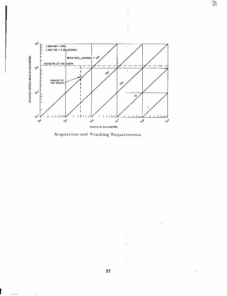
/ / / /
I o4 1 0 5 1 06 I o7 108 I o9
RANGE IN KILOMETERS
A c q u i s i t i o n a n d T r a c k i n g R e q u i r e m e n t s
37
Mission Analysis and Methodology Analysis of Mission Requirements
COMMUNICATION RANGE
Communication range for planetary probes is related to the bir th of Christ, the planet being investigated, and the type of trajectory taken to the planet.
If all other factors remain constant, the information capacity of a com- munication l ink decreases as the inverse square of the t ransmission distance. Thus, the Mars-to-Earth transmission capacity is of the o rde r of 10-6 that of the Moon-to-Earth capacity. Maintaining a given data ra te t ransmission capabi l i ty over increased range requires increases in transmitter power, transmitter aperture, receiving aperture, etc. , or some combination of these.
Communication range for a given space mission depends on the launch date and the injection energy expended as well as the objective. The Figures show communication distance at encounter versus launch date with C3, the injection energy of the escape hyperbola, as a parameter for Mercury, Venus, Mars, and Jupiter missions. The terms Type I and Type I1 refer to the two possible elliptical interplanetary transfer orbits. For Type I, the heliocentric central transfer angle is less than 180 degrees and for Type I1 it is greater than 180 degrees . Class I or I1 refers, to planetary encounter at the f irst or second intersection of the spacecraft trajectory with the planetary orbit.
38

2 0 25 30 5 I O 15 20 25 30 4 9 14 19 24 29 4 SEPT OCT NOV
LAUNCH DATE
F i g u r e A M e r c u r y 1968: E a r t h - M e r c u r y C o m m u n i c a t i o n Dis tance Versus Launch Date
I 1 I I ' . I CLASS I CLASS ll
NOTE:C, IS TWICE THE TOTAL ENERGY/UNIT MASS WITH
UNI
I
i TS rn2/sec2 x IO*
I 9 17 25 3 II 19 27 4 12 20 28 5 13 21 29 JUNE JULY AUGUST SEPTEMBER
LAUNCH DATE
F i g u r e C. M a r s 1973: E a r t h - M a r s C o m m u n i c a t i o n Dis tance Versus Launch Date
DEC
39

22 30 8 16 24 I 9 17 25 2 IO 18 26 4 12 20 JUNE JULY AUGUST SEPTEMBER' OCTOBER
LAUNCH DATE
Figure B. Venus 1970: Earth-Venus Communication Distance Versus Launch Date
1000
950
900
a50
800
750
700
650
600
550
Figure D. Jupiter 1 9 7 3 : Earth-Jupiter Communication Distance Versus Launch Date, Type I
?6
39a

Mission Analysis and Methodology Analysis of Mission Requirements
MISSION DTJRATION
Mission duration to planets is measured in years. Several possibilities exist to reduce this time but-it still remains 10 times as large as proposed Apollo Application missions.
Mission duration affects the design of communications systems for unmanned excursions primarily by imposing equipment reliability and/or lifetime requirements. For manned missions the time constraint maybe psycho1ogica11.y and physiologically limited by the crew rather than equipment reliability. There is a tradeoff between interplanetary orbit injection energy and flight time to reach a given target body in space i f a ballistic trajectory is used. Interplanetary (Mercury, Venus, Mars, and Jupi ter) flight times versus launch date for ballistic trajectories are given in Figures A through D with twice the interplanetary orbit injection energy and mass as a parameter. Figure E shows approximate transfer t imes as 2 function of solar distance. Because of the very long flight times to the outer planets via ballistic trajectories, considerable thought has been given to two alternate trajectories: Gravity assistance trajec- tories using the gravitational attraction of one or more intermediate bodies to impart energy to the vehicle as illustrated in Figure F and continuous thrust trajectories, possibly using nuclear or solar electric propulsion. Figure G compares flight times for Saturn, Uranus, Neptune, and Pluto missions using ballistic, continuous thrust, and gravi tyassis tedtrajector ies . Figure G shows, for a 273 kg (600-lb) pay- load and a sa tu rn V -Center launch vehicle, the appreciable savings in flight time achievable with constant th.rust nuclear electric propulsion and with Jupiter gravity assistance as compared to a ballistic trajectory.
Dugation of manned missions is further increased by the length of the return trip. A summary of the durations of various types of manned and unmanned missions is shown in the Tahle. It is apparent that the shortest missions, whether fly-by orbital or landing missions are con- sidered, require on the order of one year and the longest missions as long as two to three years. These flight times are longer than the pro- posed Apollo Applications Earth-orbital mission capability by a factor of ten, Mission life beyond flight time may vary from hours in the case of planetary fly-by to years in the case of a communication satellite.
40

I 70
I 6 0
I 5 0
v) 1 4 0 > a a j 130 I- I s 1 2 0
LL u.
0
I I-
110
- I O 0
90
BO
. ..
."
-t
. ..
CLASS I[ NOTE: C5 IS TWICE THE TOTAL
ENEAGY/UNIT MASS WITH UNITS m2/sec2 X lo8
1 I I I 70 I 2 0 2 5 30 5 I O 15 2 0 2 5 30 4 9 14 19 2 4 SEPT OCT NOV
LAUNCH DATE
Figure A. Mercury 1968: Time of Flight Versus Launch Date
29 4 DEC
300
280
260
24 0 f2 d - 220 Y
I- I- 4 200 J U
W I ID0 I=
160
140
120
100
F .~ _ , - . ~- " CLASS I
CLASS 11 - N0TE:Cx IS TWICE THE TOlAL
ENERGY/UNIT MASS WITH UNITS m2/sec2 X I O ~
- I c- c
I 1 C3=0.24'
I. C3=O
I 9 17 25 3 II 19 27 4 I2 20 28 5 I3 21 29 JUNE JULY AUGUST SEPTEMBER
LAUNCH DATE
Figure C. Mars 1973: Time of Flight Versus Launch Date
41

22 30 8 16 2 4 I 9 17 25 2 IO 18 2 6 4 12 2 0 JUNE JULY AUGUST SEPTEMBER OCTOBER
LAUNCH DATE
Figure B. Venus 1970: Time of Flight Versus Launch Date
1300
1200
I100
1000 In
0 k e - 900
z 800 LL -I
LL 0 w
I-
700 I
600
500
400
300
CLASS II NOTE: C3 IS TWICE THE TOTAL
ENERGY/UNIT MASS WITH
UNITS m'/sec'x lo8
LAUNCH DATE
Figure D. Jupiter 1973: Time of Flight Versus Launch Date, Type I
41a
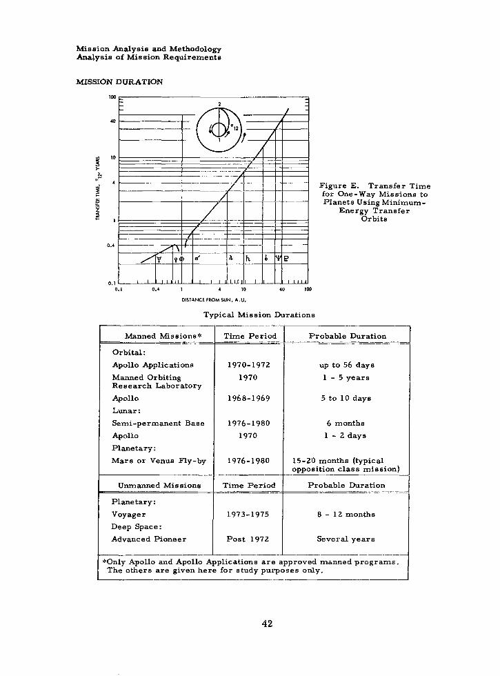
Mission Analysis and Methodology Analysis of Mission Requirements
MISSION DURATION
IW ... . "
10
4
I
0.4
0. I 0 . I 0.4 I 4 10 40 100
DISTANCE FROM SUN, A.U.
Typical Mission Durations .-
Manned Missions*
Orbital: Apollo Applications Manned Orbiting Research Laboratory Apollo Lunar : Semi-permancnt Base Apollo Planetary: Mars 01 Venus Fly-by
Unmanned Missions c
Planetary: Voyager Deep Space: Advanced Pioneer
Time Period
1970-1972 1970
1968-1969
1976-1980 1970
1976-1980 "~
Time Period F_
1973-1975
Post 1972
Figure E. Transfer Time for One-way Missions to Planets Using Minimum-
Energy Transfer Orbits
Probable Duration ""
up to 56 days 1 - 5 years
5 to 10 days
6 months 1 - 2 days
15-20 months (typical opposition class mission)
Probable Duration -_
.___" .~ -
8 - 12 months
Several years
I *Only Apollo and Apollo Applications a r e approved manned programs. The others are given here for study purposes only.
42

TRAJECTORY DATA (GRAVITY ASSIST): LAUNCH YEAR. 1977 IDEAL VELOClh' = 16.500 WSEC TIME TO JUPITER = 502 DAYS TOTAL TRIP TIME = 1072 DAYS
TRAJECTORY DATA (DIRECT):
TRIP TIME = 12W DAYS IDEAL VELOCITY = 17,200 WSEC
JUPITER'S ORBIT
POST-ASSIST HELIOCENTRIC TRAJECTORY
\ \ \ 1 \
ORBIT EARTH'S \
EARTH AT
Figure F. Jupiter Gravity Assisted Saturn Fly-By Mission
OUTER PLANETS' MISSIONS FLIGHT TIME COMPARISON
20 LB - 9.05 K G 40 LB - 18.1 K G
a = 40 a = 20
a 40 a = 20
PAYLOAD - 600 LBS D -DIRECT BALLISTIC SATURN V
G A - GRAVITY ASSIST CENTAUR AT JUPITER I
T-THRUSTED I a - 20 LBS/KW (500 KW) a - 40 LBS/KW (250 KW)
SATURN IB PACE CRUISER
a = 4 0 a = 20 a = 4 0
a = 20
NOT POSSIBLE TO G O DIRECT G O PLUTO WITH SVC N O DATA FOR GRAVITY ASSIST
SATURN URANUS NEPTUNE PLUTO
' .
Figure G. Comparison of One-way Flight Times to the Outer Planets Using Ballistic Gravity
Assisted, and Thrusted Trajectories
43

Mission Analysis and Methodology Analysis of Mission Requirements
COMMUNICATION SYSTEM WEIGHT RESTRICTIONS
Communication system weight restriction is a compromise between the system per- formance requirements and the available weight which i s in turn dependent upon the type of booster used. ~ _ _ ~ ~ . . . . . - - - . .
Permissible payload for a given mission is dictated by launch vehicle capability and allocation of that payload among the various spacecraft systems is determined by mission objectives. The fractional part of the payload comprised by the communication system wi l l vary depending on the required data rates and transmission range. Payload capabili t ies of present and projected launch vehicles are depicted in the Figure. I t can be seen that the payload weight which may be launched on a given mission (i. e., at a specified characteristic velocity) is a discrete ra ther than a continuous function. Hence vehicles having weights intermediate between the payload capabilities of two launch vehicles may be increased in weight to the payload of the next largest launcher without penalty. Thus for some payload weights, additional weight may be a non-critical burden. An example of such payload weight quantization is the rather wide gap in payload capability between Saturn iB/Centaur and Saturn V.
44

LARGE ORBITING LAB
APOLLO
MEDIUM ORBITING L A B
EXTENDED APOLLO MOL
GEMINI, VOYAGER
TIROS
TELSTAR. RELAY SYNCOM I \ ATLAWCENTAUR
I
LUNAR EQUATORIAL SYNCHRONOUS
TRANSFER EARTH ORBIT
10'
0.1-AU SOLAR PROBE
0.05-AU SOLAR PROBE- i %SOLAR SYSTEM
ESCAPE
SATURN IB/ CENTAUR
L 1 I
... :... . : .:..:
.: :::: .... .... .::: ... . . . . , . ..:. .:. ::.. .. ..: .: .:: , . :..:x.::: .: ..... :. .. ,. . . .. .:. .... ... .:. .... .... :.:.. .:.:.. .: ..., ..:...
20 25 30 35 4 0 4 5 5 0 5 5 60 65 70 75 80
6 9 1 2 15 18 2 1 2 9
CHARACTERISTIC VELOCITY (THOUSANDS OF FEET PER SECOND)
I I I I I I I
C H A R A C T E R I S T I C V E L O C I T Y ( K I L O M E T E R S P E R S E C O N D )
Launch Vehicle Capabilities - Payloads and Destination
The horizontal characteristic velocity scale shows velocity a vehicle needs at 185 Km altitude (not orbit) to reach destination, assuming a minimum energy trajectory.
45

Mission Analysis and Methodology Analysis of Mission Requirements
MISSION OPPORTUNITIES
Planetary mission opportunities depend upon the synodic period of the planet and have acceptable durations of 1 to 3 months.
In reality, feasible launchings can occur only for small time intervals (1 -3 months) whenthe relative positions of Earth and the target p lanet are such that the velocity requirements for ball ist ic transfers can be reason- able achieved by modern boost vehicles. These intervals occur once during each synodic period of the planet. A synodic period is the time interval required for the Earth and target p lanet to attain the same helio- centric longitude.
Thus, favorable launch opportunities occur approximately every 1. 6 years for Venus, every 2. 1 yea r s fo r Mars , every 0 . 3 year for Mercury and every 1. i years for Jupiter. The Figure shows the opportunity pe- riodicity for these planets along with the approximate injection energy requirements . Also l is ted in the figure is the next few opportunity dates for each of these planets.
46
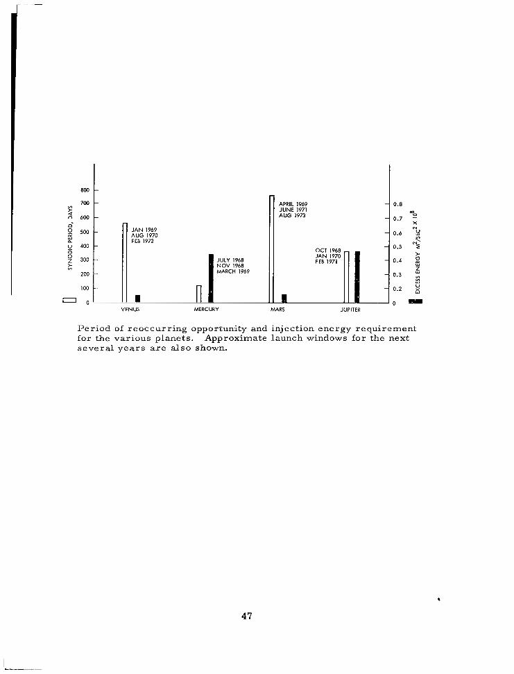
AUG 1970 JAN 1969
FEB 1972
I JULY 1968 NOV 1968 MARCH 1969
". a n
0.8
0.7 ' X
0.6 M
0.5 Z
0.4 2 >
0.3 z
m
N
N?
v1 Y
0.2 g 0 -
VENUS MERCURY JUPITER
Period of reoccurring opportunity and injection energy requirement for the various planets. Approximate launch windows for the next several years are a lso shown.
47


. ~ ......... .._
MISSION ANALYSIS AND METHODOLOGY
Methodology for Optimizing Communication Systems
Page The Purpose for a Communications Methodology . . . . . . . . . . . . . . . . . . . . . . . . . . . . . . . . . . 50
Major System Parameters Used in the Methodology . . . . . . . . . . . . . . . . . . . . . . . . . . . . . . . . . 52
Types of System Classified in the Methodology . . . . . . . . . . . . . . . . . . . . . . . . . . . . . . . . . . . 54
Keystone Optimization Procedures Used in the Methodology . . . . . . . . . . . . . . . . . . . . . . . . . . . 56
Structural Detail of Methodology Implementation . . . . . . . . . . . . . . . . . . . . . . . . . . . . . . . . . . . 58
System Burden Parameters . . . . . . . . . . . . . . . . . . . . . . . . . . . . . . . . . . . . . . . . . . . . . . . 62
Basis for Present Burden Relations and Constants . . . . . . . . . . . . . . . . . . . . . . . . . . . . . . . . . . 66
Uncertainties in Present Burden Relations . . . . . . . . . . . . . . . . . . . . . . . . . . . . . . . . . . . . . . 70
49
"

Mission Analysis and Methodology Methodology for Optimizing Communication Systems
THE PURPOSE FOR A COMMUNICATIONS METHODOLOGY
A comprehensive communications methodology has been developed to provide impartial evaluation of communication systems using weight and cost as c r i te r ia .
The previous two sections have described scientific objectives and com- munications requirements for deep space missions. These requirements must be related to communications systems in a logical and impartial manner in order to evaluate fairly the several communication system choices available. In par t icular , it is desireable to evaluate both laser and radio communications systems using optimum configurations for each. The importance of determining optimum systems for comparison is clearly required, otherwise system designs may be formulated which lead to unfair comparisons.
A means for generating such comparison has been developed during this contract. It is based upon two cr i ter ia , that of determining the lightest weight system to provide a given performance and that of providing the least expensive system to provide a given performance. This has been called a "Communications Methodology". It has been programmed for a computer to provide optimum values for all the key design parameters of a communications link.
Subsequent topics describe the salient features of the Communications Methodology and give examples of its use. The Methodology then forms a bas is of analysis which uses as g r o s s inputs 1 ) mission objectives and requirements and 2 ) detailed descriptions of communicati'on constraints and components. The communications constraints are discussed in this Volume, Volume I1 in the form of Communication Theory, and in Volume IV in t e rms of Atmospheric Limitations and Existing Ground Facilities. Communication components are discussed extensively in Volume 111. These include such components as transmitter power sources, antennas, detectors, etc. Communications constraints and components are described for both radio and optical systems.
The topics which follow in this section illustrate how the methodology is formed, the rationale it uses, the practical data it required (burdens) and examples of i ts use.
50

Mission Analysis and Methodology Methodology for Optimizing Communication Systems
MAJOR SYSTEM PARAMETERS USED IN THE METHODOLOGY
Four major sys tem parameters are defined which may be used to express the weight or cos t of an entire communication l ink. These parameters are: The transmitter power, the transmitter antenna gain, the receiver antenna gain, and the receiver f ield of view.
___ .~ . _" - . .. . " .~ ~ _ _ _
The complex relationships between the design parameters of communica- tion systems and their fabrication cost, weight, volume, power require- ment, etc. , create the need for a unified approach to the optimum design of communication systems. An optimization methodology is needed which provides the system designer with the optimum values of the major parameters of a communication system. Major system parameters have the characterist ic that al l communications l ink parameters may be expressed in terms of one of them. The major system parameters are:
Transmitter antenna diameter (or gain) Receiver antenna. diameter (or gain) Transmitter power Receiver field of view
The optimization methodology is applicable for optical as well as radio systems. In principle, any type of modulation or demodulation can be handled i f some suitable performance criterion is available. The opti- mization procedure for the most common and practical combinations of digital modulation and detection techniques are documented in this report . For these systems the performance cri terion is the probability of detect ion error .
Basically, the optimization procedure is to develop system cost relation- ships as a function of the values of the system parameters. These cost relationships include the fabrication cost of the system components, the cost of placing the components aboard a spacecraft, and any other per- tinent system costs. This phase of the optimization procedure is, in many re,spects, the most difficult since in many cases it requires tech- nological predictions. However, a great amount of parametr ic cost burden data has been gathered for many system components (See a sub- sequent topic in this section on burdens). With the cost relationships developed, the total system cost is minimized as a function of the values of the major system parameters under the constraint that the perform- ance cr i ter ion is achieved.
The communication component burden relationships employed in the optimization procedure may be modeled by power series or be specified numerically. The only requirements are that the burden relationships be monotonic, single-valued, piece-wise differentiable functions of the system parameters. These conditions are usually fulfilled for the four major system parameters listed previously. The conditions are gener- ally not met when attempts are made to express burdens as a function of transmission wavelength.
As an introduction to the relationships between communication parameters and weight or cost, the following paragraphs are given.
Transmitter Antenna. The weight and fabrication cost of a t ransmi t te r antenfia system are dependent upon the transmitter antenna diameter. A transmitter antenna is usually designed to operate as close to the
52

diffraction limit as possible to achieve the greatest spatial power density at the receiver for a given transmitter aperture diameter. For small t ransmit ter aper tures , the weight is proportional to the antenna area, and hence to the square of the aper ture diameter . For larger s ize aper tures , as s t ructural supports are added to maintain the rigidity required for diffraction limited operation, the weight dependence becomes volumetric.
Receiver Antenna. The weight and fabrication cost of a receiver antenna system are dependent upon the receiver antenna aperture diameter. At optical frequencies receiver antennas are not normally designed to be diffraction limited, and hence construction and mechanical support toler- ances need not be as stringent as for a transmitter antenna.
Transmitter Antenna Pointing System. The transmitter antenna pointing system consists of a gimballed support unit, which points the transmitter antenna toward the receiver. The weight of the transmitter antenna pointing system is relatively insensitive to the transmitter pointing accuracy. Its weight is proportional to the weight of the t ransmit ter antenna, which in turn has a weight dependent upon the t ransmi t te r antenna diameter. The fabrication cost of the transmitter pointing equipment is inversely proportional to the transmitter pointing accuracy. The pointing accuracy is usually specified as a fixed percentage of the transmitter beamwidth. Since the transmitter antenna is diffraction limited, the fabrication cost is proportional to the transmitter aperture diameter. The electrical power requirement for the transmitter antenna pointing system is primarily dependent upon the weight of the transmitter antenna.
Receiver . . - Pointing System. The weight of the receiver pointing system is relatively insensitive to the receiver pointing accuracy. Its weight is proportional to the weight of the receiver antenna, which is itself depend- ent upon the receiver aperture diameter. The fabrication cost of the receiver pointing equipment is inversely proportional to the receiver pointing accuracy, which is a fixed percentage of the receiver field of view. The power supply requirement for the receiver pointing system is primarily dependent upon the weight of the receiver antenna.
Transmit ter . For a given transmission wavelength, within limits, the weight and fabrication cost of a t ransmit ter are dependent upon the transmitter power. The electrical input power requirement is directly proportional to the transmitted power.
Transmitter System Power Supply. The fabrication cost and weight of the electricaT power supply and conversion equipment at the t ransmit ter are dependent upon the electrical power requirements of the transmitter antenna pointing system, transmitter, and modulator.
Receiver System Power Supply. The fabrication cost and weight of the electrical power supply and conversion equipment at the receiver are dependent upon the power requirements of the receiver pointing system and communications receiver equipment.
~ -. - "
53

Mission Analysis and Methodology Methodology for Optimizing Communication Systems
TYPES O F SYSTEM CLASSIFIED IN THE METHODOLOGY
Communication systems are classified by: transmission wavelength, modulation method, demodulation method and dominant noise in the detector.
The communications methodology developed is intended to be comprehen- s ive , so that a great variety of sys tems may be examined. The systems which may be considered are taken from the following classifications.
0 Transmission wavelength
0 radio 0 optical
0 Modulation method
0 PCM amplitude modulation 0 PCM polarization modulation 0 PCM frequency modulation 0 PCM phase modulation
0 Demodulation method
0
0 di rec t 0 heterodyne 0 homodyne
Types of noise
0 thermal 0 background radiation 0 shot
A division between optical and radio systems is commonly taken at awave- length of 100 microns. For wavelengths shorter than 100 microns the trans - mitter is usually a laser , the antennas are made of polished reflectors or transparent lenses, and the carrier demodulator is a photodetector. At the radio wavelengths a var ie ty of transmitter oscil lators are avail- able, the antennas are generally metal reflectors, horns, or wire assemblies, and the detector is a nonlinear electrical element.
Not all combinations of modulation and demodulation methods are feasible at all transmission wavelengths but rather sets usually results from practical considerations. For instance, polarization modulation is limited to the optical region because of difficulties in constructing radio frequency polarization modulators. Also radio frequency phase modu- lation systems must employ a homodyne receiver to perform optimum demodulation.
At radio frequency, noise is principally caused by two physical sources, thermal noise at the antenna load and background radiation from external sources . Both types of noise may be modeled by Gaussian statist ics. However, optical receiver noise is.caused by two sources: 1) thermal noise of the photodetector load resistor and resistive elements within the detector, 2 ) by detector shot noise which is caused by the randomness
54

_" ." . . .. .
of electron emissions induced by laser carrier radiation, background radiation, and detector dark current. Shot noise is modeled by Poisson statistics. In an optical direct detection receiver, if the photodetector has an internal current gain mechanism, detector shot noise is usually dominant, otherwise thermal noise predominates. In a heterodyne or homodyne optical receiver the local oscillator power can be made large to achieve shot noise limited operation even without photodetector gain.
For the Communication Methodology optimization analysis, communica- tion systems have been divided into four types which are descr ibed below.
ROPS - Radio communication Optimization system with Stops. This system is thermal and background radiation noise l imited and uses Gaussian detection statistics.
TOPS - Thermal noise optical Optimum communication system with Stops. This system uses direct detection, is thermal noise l imited and has Gaussian detection statist ics.
SOPS - Shot noise optical Optimum communication system with Stops. This system uses direct detection is shot noise l imited and has Poisson detection statist ics.
HOPS - Heterodyne optical Optimum communication system with Stops. This system uses heterodyne or homodyne detection, is shot noise limited and has Poisson detection statist ics.
These four types of communication systems have been incorporated into the computer implementation of the optimization procedure. They are conveniently implemented as separate parts since the detection processes differ.
55
Mission Analysis and Methodology Methodology for Optimizing Communication Systems
KEYSTONE OPTIMIZATION PROCEDURES USED IN THE METHODOLOGY
The heart of the .optimization procedure consists of partially differentiating the functional relationships describing the four major system parameters and solving for optimum values by use of Lagrange multipliers.
~-~~ -~ . . ~
Let x, y, z, w represent a s e t of four physica1,parameters of the com- munication system to be optimized, e,. g. , transmitter antenna gain or diameter, receiver antenna gain or diameter, transmitter power, and receiver field of view. The probability of detect ion error , P, may then be expressed in terms of the sys tem parameters as
p = f l (x, y, z , w) (1 1
Likewise, the total system cost, C, is another function of the system parameters .
c = f 2 (x, y, z , w)
Let PR be the required probability of detection error. Then, by the method of Lagrange multipliers, to minimize the total system cost and achieve PR, the dummy function C ' is formed
C' = C t A (PR - P)
Where A is the Lagrange multiplier. Now, setting the partial derivatives of C' , with respect to the system parameters, equal to zero yields.
Equating then ' s g ives a se t of six characterist ic equations.
'Schechter, R. S., The Variational Method in Engineering, McGraw- Hill, New York, 1967.
56
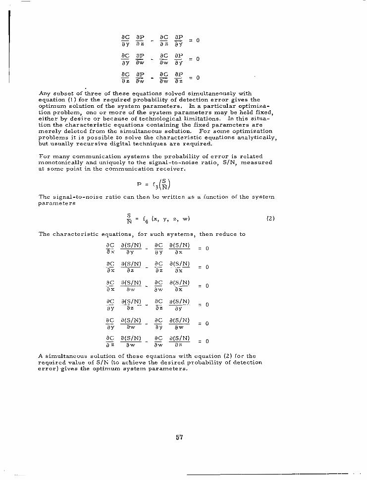
a c a p " _ " ac a p = 0 ay aw aw a y
a c a p ac a p = a z aw aw a z -""
Any subset of th ree of these equations solved simultaneously with equation (1) for the required probability of detection error gives the optimum solution of the system parameters . In a particular optimiza- tion problem, one or more of the system parameters may be held fixed, e i ther by desire or because of technological limitations. In this situa- tion the characteristic equations containing the fixed parameters are merely deleted from the simultaneous solution. For some optimization problems i t is possible to solve the characteristic equations analytically, but usually recursive digital techniques are required.
For many communication systems the probability of e r r o r is related monotonically and uniquely to the signal-to-noise ratio, S/N, measured at some point in the communication receiver.
P = f 3 ( G )
The signal-to-noise ratio can then be wri t ten as a function of the system parameters
The characteristic equations, for such systems, then reduce to
ac a ( s / N ) a c a ( s / N ) = a x ay a y a x
a x a 2 a 2 ax - aC B(S/N) ac ~ a(S/N) =
ac a ( s / N ) ac B(S/N) = a z aw aw az - ~- - ____
A simultaneous solution of these equations with equation ( 2 ) for the required value of S/N (to achieve the desired probability of detection error) .gives the opt imum system parameters .
57

Mission Analysis and Methodology Methodology for Optimizing Communication Systems
STRUCTURAL DETAIL O F METHODOLOGY IMPLEMENTATION
Typical equations for the detailed methodology are given. A complete listing of these equations is given in Appendix A.
Previous topics have i l lustrated the purposes and approach used to develop an optimized communication methodology. It is the purpose of this topic to i l lustrate the level of detail required in this implementation. Since this implementation contains a considerable amount of repetition, the majori ty of the detail is relegated to Appendix A of this volume.
The communication methodology optimizes the communication parameters such that either the lightest or least expensive communication system is derived, within the constraints imposed. It is therefore necessary to represent the various component parts of a communication system in t e r m s of the weight and cost. (Additionally relationships for power have also been formulated. )
The following communication systems components have been represented in t e rms of weight and/or cost: transmitter antenna, receiver antenna, transmitter acquisition and pointing system, receiver acquisition and pointing system, the transmitter modulator, the receiver demodulator,
heat rejection system. These several relationships have been combined, the net result relates the complete communications system to four major system parameters which are: the transmitt ing and receiving antenna diameters, the transmitted power and the receiver f ield of view.
As an i l lustration of the equations used, the relationships of the t rans- mitter antenna are listed below as is one of the four composite equations which illustrates the detail and format of the equations given onlyfunc- tionally in prior topics.
Transmitter Antenna Burdens
' the receiver power conditioning, the transmitter, and the spacecraft
The weight and fabrication cost of a transmitter antenna are proportional to the transmitter aperture diameter. The transmitter antenna weight is
and the fabrication cost is
CgT = CKT + KgT (dT) mT
where
dT = t ransmi t te r aper ture d iameter
KdT = constant relating transmitter antenna weight to transmitter aperture diameter.
KeT = constant relating transmitter antenna fabrication cost to t ransmit ter aper ture diameter .

WKT = transmitter antenna weight independent of t ransmi t te r aper ture diameter .
CKT = transmitter antenna fabrication cost independent of t ransmit ter aper ture diameter .
nT = constant
m T = constant
The total cost associated with transmitter antenna includes the fabrica- tion cost and the cost of placing the weight, WdT, aboard a spacecraft . Thus,
where
K = cost per unit weight for spaceborne equipment S The cost, CT, of the transmitter antenna and associated tracking equip- ment which 1s dependent upon the transmitter aperture diameter is a s follows.
CT E
t
s"-f \" fabrication fabrication weight cost weight cost of cost of cost of t ransmit ter t ransmit ter transmitter transmitter antenna tracker tracker antenna
weight cost of t ransmi t te r tracker power s UPPlY
In simplified form
fabrication cost of t ransmit ter tracker power supply
59

Mission Analysis and Methodology Methodology for Optimizing Communication Systems
STRUCTURAL DETAIL O F METHODOLOGY IMPLEMENTATION
where
- - KnT - KdT 1.s [' -t KWAT]t KPQTKWAT [.ST ' K S K ~ S T ] )
where:
KAT = constant relating transmitter tracking equipment fabrication cost to transmitter beamwidth
h = transmitted wavelength
gt = a constant
K w A T = constant relating transmitter tracking equipment weight to transmitter antenna weight
KwST = constant relating transmitter power supply weight to power requirement.
K p Q T = constant relating transmitter acquisition and track equipment power requirement to equipment weight.
KST = constant relating transmitter power supply fabrication cost to power requirement.
60

Mission Analysis and Methodology Methodology for Optimizing Communication Systems
SYSTEM BURDEN PARAMETERS
System "burdens" are the constants which are used to relate communication parameters e. g. the transmitter antenna diameter, to weight or cost. Numerical values for these burdens are given. -_ -
Associated with each major component of the various communication systems considered in the study are two equations that express the com- ponent weight and cost, respectively, as functions of the most appro- priate communication system variable, dT, dR, PT, o r eR. For example, spacecraft prime power supply weight and cost are expressed as functions of transmitter output power, PT; transmitter antenna weight and cost are expressed as functions of transmitter antenna diameter, dT. These burden relations relate communication system configuration specified by a se t of values of the system variables) to the corresponding system weight and cost. The optimization program incorporates these burden relations and the appropriate expressions relating the four major system variables, dT, dR, PT, and 8R to the data transmission rate, RB. Using these relations, the computer calculations determine the set of values of dT, dR, PT, OR that correspond to a minimum weight or minimum cost system at each specified data transmission rate, RB. Thus it may be seen, that the efficacy of the computerized procedure for determining an optimum system configuration and the sensitivity of that configuration to variations in the cost or weight burdens depends criti- cally on the correctness of the assumed burden relationships.
Confidence in the burden relationship presently being used varies, depending strongly on the component in question. As a general rule, cost burdens are considerably more nebulous than weight burdens. For some components such as photovoltaic power supplies, space radiators, launch costs, and perhaps antennas and optical apertures; the relation- ships can be expressed with reasonable certitude. On the other hand, burden relations for space qualified transmitting sources (both optical and higher power microwave) and the precise pointing systems required with the narrow laser beamwidths are known with less confidence.
The difficulties associated with accurately assessing these relationships stem primarily from two considerations:
1. Component complexity or configuration that does not lend itself to expressing the associated burdens as functions of a single system variable.
2. Fai lure of existing technology to provide space qualified components of the requisite performance with the result that burdens must be based on a time extrapolation.
The component burden relations presented here will continue to evolve in the path of technological advance and fuller understanding of the many diverse technologies represented.
The component burden relationships presently used are summarized in Tables A and B. Table A shows components for which the burden con- stants are relatively independent of mission destination. For each component, the assumed equations relating the associated variable system parameter and the component weight or cost burden are given
62

in the left column. * In adjacent columns, the values of the constants appearing in these burden equations are listed for the various communi- cation system optimization programs. Table B shows components that strongly mission dependent burden constants, principally the launch vehicle and prime power supply. Launch vehicle costs are based on the Saturn V Centaur combination which results in a lower cost per pound of payload than smaller launch systems when the full payload capabilities of that system can be utilized.
..* ~. ' The nomenclature for these equations is defined in Appendix A of this volume.
63

Mission Analysis and Methodology Methodology for Optimizing Communication Systems
SYSTEM BURDEN PARAMETERS
Table A.
Receiver Anrenna
c d R 2 CKR t KeRdR m R
Transmitter Acqulsl l ion and
Pointing S y s t e m
wQT = W B T "ATWdT
CQT = CAT t KAT(A/dT) -qT
'QT ' K P ~ ~ " ' ~ ~
Receiver Acquislt lon snd Polnling s y s t e m
-qR CQR = 'AR + K ~ ~ ( e ~ ' 'QR = K P ~ ~ W~~ Modulation B u r d e n
W M = W K M t K M R B
'M = C~~ + K ~ ~ R ~
'M ' K ~ ~ W ~
Dernodulatwn Bmtrden
WD = W K D t K D R B
SD 2 CKD t K F D R B
P = K D P D W D
Rece lver Power Condllronlng
' S R = c~~ + K ~ ~ P ~
Spacecraft Transmi l t er
W p T = WKp t KWTPThT
cpT = cKp + K ~ ~ P ~ ~ T
PST = PT/ke
SpacecraI l Heal Rejeclion
1- Present Component Burden Relations Not
Directly Mission Dependent
" ~~
K e T
KdT
'KT
W K ?
m T
T
K e R
'KR
M R
K~~
K W A
KpQ.
'AT
w~~
9.I
K~~
'AR
q R
K F M
K M
PM
CKM
'Iy Khl
K F D
K D
K P D
'KD
W~~
"SR
'K F
KPT
K W T
cKP
'"KP
i T hT
ke
K H KX
'=KH
W~~
~"
T A = 10. 6p
HOPS
14
0 .012
20 x 1 0 3
5
2
2. 2
8 75
25 x 10)
2
0 .11 r 10
0.1;
0 . 4 8
0 . 4 x 10⁶
40
0 3
o 71 x l o 5
0 . 2 x 10⁶
0 3
0.5 x
0.3 x 10-6
5
15 x l o 3
s o
0 . I
0 . 2 x 1 0 - 6
2 7 . 5 x 10³
3. 33
55
2 5 . 0
5 x 10³
1 . 4 3
2
I O lo3
25
1
1
10
1.97
2 . 5 x 10⁻²
13 .8 x I O 3
0
. . . - . - . .
TOPS A = 10. 6p
~ " ~ ~.
1 4
0.012
20 x 1 0 3
5
2
2 2
8. 1 5
25 x I O 3
2
0 71 x 10
0 . 1 3
0 . 4 8
0 4 x I O 6
40
0. 3
o . l l l o 5
0 2 x I 0 6
0 3
0 5 x l o - :
o 3 x IO-^ 5
15 x I O 3
I O
5 5 x 10⁻⁵
I . I x l a - '
3. 33
15 x l o 3
30
25. 0
5 x 1 0 )
1 . 4 3
2
x
25
I 1
10
2. 5 x IO"
1 .97
1 3 8 x IO3
0
-
gram
SOPS A = 0. 511
"_ 14
0 . 0 1 2
20 x 103
5
2. 2
8 1 5
25 x I O 3
2
0 71 x 10
0. I 3
0 48
0 .4 x 106
40
0. 3
0 . 1 1 x 1 0 -
0.2 x 10⁶
0 . 3
7. 5 x 10..
5. 0 x 10-t
7 . 5 x 10³
5
5
5 . 5 x 1 0 -
1 . I x I O "
3 . 33
I 5 A I O 3
30
25. 0
5 x l o 3
150
51
I O x l o 3
40
I I
0. I
0. 58
I. 1 x 10-c
3 . 8 x 1 0 )
)
- .. - -. .
ROPS L = l Jcm
. . . . .~ "" ~, - 4 . 0
4 . 3 2 x
5. o x 103
0
2
2
6 4
105
o 71 x l o 5
2 1
0 . 15
I O
0 . 14 x 10'
15
0. 3
Cornblned wlrh rece iver Lnlenna burdens
120
0 1
I O x 10)
0. 1
1
I
25
0.58
I. 1 x 1 0 - 2
1 3 . 8 x IOt3
0
. - - . -. .
I
64

Table B. Mission Dependent Burden Relations (Applicable to All Computer Programs - HOPS, TOPS, SOPS, and ROPS)
I . T r a n s m i l l e r Power Supply
CST E CKE + K ~ ~ P ~
KST. d o l l a r s Cons tan t per watt
M e r c u r y f l y b y 43 (orienled aolar panel1
Venus flyby ( o r i e n l e d s o l a r p a n e l )
Near E a r l h miarrlons
unecl ipsedl ( o r i e n l e d aolar panel -
Mars flyby (oriented solar panel1
5 3
112
IO d e q r e e s
0 . 04
0 . 04
0 . 05
0 .11
0. b25
0. 7
.
2. System Welghl Cost:** C)vs = KSWS
0
1 . 2 x 10⁶
0
DI!Jla,lCC f rom Sun
(or E a r l h t l -~
I 5 PSJ
208. 000 "rnt
5.2 AU
0 . 2 AU
0. I 2 AU
1 O A U
1 . 0 A U
4 0 A U
40 AU
"--""t---"- Transtr
Tune .. .. ~ ..
1 5 0 d a y s
LOO h o u r s
750 d a y s
60 daye
7 6 d a y s
200 d a y s
200 days
4000 days
4000 days
Standard Saturn v Ce"l"ar
86.000
85. ooo
36.000
14.000 5, 500
12,000
I , 2 5 0
13. 000
8. 500
Satvrn v Upratcd
Cen1uar
9 7 , 0 0 0
. . ~
95. 500
44.000
1 5 , 0 0 0
b. 000
1 2 . 5 0 0
3,500
1 4 . 0 0 0
9 , 0 0 0
__..
T
WKE. pounds
0
0
0
0
400
0
O p e r a t e d saturn v c c n t a u r
'Clylc, 1. D., and Wimmer . R.E., "Rpacror~rl~ermoelecrricPower SystemB for Unmanned Salcl l l te Appl i ca r iune . " P roceed ings of the l n t e r s o c ~ e l y Energy Convcrston Conference, Los Angeles, Cali lornra, S r p l e m b c r 2 6 - 2 8 . I96b.
Baaed on payload data lrorn Saturn V M i s a l o n Planner 's t iulde. Douglas A l r c r a f f Co.. and B total vehlcle and launch c o e l of *i
$ 1 5 3 mill ion. " * C
Incl inat ion between vehicle t r a l ec lo ry and echptic plane.
tDl6rance from E a r l h .
65

Mission Analysis and Methodology Methodology for Optimizing Communication Systems
BASIS FOR PRESENT BURDEN RELATIONS AND CONSTANTS
Weights and costs are based upon the best estimates for space qualified hardware developed from the most advanced existing technology.
~~ ~ .. - - ."
The general assumptions on which the burdens of the previous topic are predicated are as follows:
1. Weights and costs are based on best estimates for space qualified hardware developed from the most advanced existing technology; i. e. , that which might, with sufficient emphasis, find a space application within several years.
2. Costs cited are based on production costs for limited production (10 uni t s o r l ess ) but do not include basic research or develop- ment costs.
Additionally, it is appropriate to mention some of the specific assump- tions underlying the burdens for each of the component areas, since in most instances each burden is based on a specific type or configuration of component either dictated by the constraints of the application or indi- cated by considerations of availability, reliability, weight, or cost. Specific comments follow relative to burden relationships.
Spacecraft Transmitter Antennas and Primary Optics. Spacecraft microwave antenna weight and cost burdens are best es t imates for space erectable rigidized inflatable dishes and are felt to be reasonably accurate up to diameters of 35 feet.
Spacecraft primary optical aperture weight and cost burdens are based on available information for beryllium sandwich mirrors. It is m o r e appropriately a first order approximation for apertures up to 120 inch diameter . A more sophisticated weight analysis will take into account the weight dependence on operating wavelength for specified surface accuracy.
Receiver Antennas and ApertuF- Microwave receiver antenna costs are considered collectively with receiver pointing and tracking system and receiver power supply costs based on published costs of the 85-foot and 210-foot DSIF s i te of $1 million and $12 million, respectively.
Optical receiver aperture cost is based on available information on fused sil ica, cored center, sandwich type mirrors constructed according to the technique developed by Corning Glass Works.
Spacecraft Transmitter Acquisition and Pointing. Microwave transmitter acquisition and pointing cost is based on a three gimbal system s imilar to that proposed by Hughes for the Apollo LEM with greater angular acceleration (0. 01 rad/sec2) and angular rate 1°/sec capabili ty than required for a deep space vehicle.
Optical transmitter acquisition and pointing system weight is based on the two gimbal telescope system studied by Perkin-Elmer with internal fine pointing to 0. 1 pr by a t ransfer lens and using Ris ley pr isms for point ahead.
66
Receiver Pointing. For the microwave system receiver pointing and tracking costs are consolidated with the receiver antenna and power supply costs.
Optical system receiver pointing and tracking costs were assumed to have the same variable cost dependence as the spaceborne system.
Modulation. For the microwave system, modulation weight and cost associatedwas assumed negligible, since it occurs at very low power levels.
_"
Optical modulators were assumed to be driven by solid state circuitry to a level at least half their ultimate modulating capacity with phase or frequency modulation for the heterodyne system and intensity or polari- zation modulation for photodetection systems.
Demodulation. Negligible weight and cost burdens associated with microwave demodulation are combined with the receiver antenna burdens.
Demodulation for the optical heterodyne system is by a mixer cooled to 100°K. The other optical systems use photodetector receivers.
Spacecraft Thermal Control. Radiator costs and weights are best esti- mates by a leading environmental control company for oriented active fin and tube aluminum radiators. They depend on the radiator tempera- ture, hence on the transmitting source used. At present rf power levels radiation from the spacecraft structure with conductive coupling to the transmitter source suffices. Weights as l isted for the various systems are based on a radiator temperature equal to the operating temperature of the associated transmitting source.
Spacecraft Transmitter Sources. Present microwave weight and cost burdens are based on capabilities of systems using the popular scheme of paralleling traveling wave tube amplifiers to achieve required output powers (as well as enhanced reliability and dispersion of hea t sources) . In this situation, transmitter system weight and cost are approximately linearly proportional to transmitter power since both are proportional to the number of paralleled tubes. Transmitter source cost and weight burdens include those associated with the required power conditioning electronics and its efficiency includes conversion losses.
Optical transmitt ing source burdens are known with far less confidence due to the non-existence of space qualified lasers. Present burdens for X = 0. 5p argon laser sources were extrapolated f rom a 2-watt airborne unit developed by Hughes Research Laboratories. Included are the weight (10 lb/kw) and cost of required power conditioning equipment based on a laser efficiency of 0. 1 percent and a power conditioning effi- ciency of 80 percent. Due to their low efficiency, liquid cooling is required for all argon lasers (typically coolant is flowed between the concentric solenoid and discharge tube). The portion of the cooling loop integral with the laser is included to arrive at the weight burden. It is significant to the evaluation of the associated radiator burdens that a maximum safe operating temperature of 300°F (limited by safe opera- tion of the solenoid) is assumed.
67

Mission Analysis and Methodology Methodology for Optimizing Communication.Systems
BASIS FOR PRESENT BURDEN RELATIONS AND CONSTANTS
Present burdens for A = 1 0 . 6 ~ C 0 2 laser sources were in fer red f rom the bes t es t imates of projected weights and costs of space qualified devices in the 10 to 100 watt output power range. Power conditioning system weight ( 10 lb/kw or 4. 55 kg/watt) and cost are included in the burdens based ona laser eff ic iencyof 10 percent and power conversionefficiencyof 80 pe r - cent. Since CO2 laser efficiency(hence output power) drops sharplywithin- creased temperature, liquid cooling might be required at power levels of interest for space transmitt ing sources. The usual technique is to enclose the discharge tube within a concentric cooling jacket and flow coolant through the annular passage between them. This configuration has been assumed in including the integral cooling jacket weight in the C02 source weight burden.
Although the C02 lasers on which the 10. 6p burdens are based are not themselves capable of the single frequency-single wavelength operation required for heterodyne systems, such devices wil l have comparable character is t ics s ince the C02 laser is near ly as efficient at a single wavelength as when operating in a multiwave length mode. Single frequency-single wavelength C02 lasers have achieved 10 to 15 watts in laboratory operation and 100-watt single frequency devices are held attainable with present techniques.
Spacecraft Prime Power Sources. In general, the choice of prime power source type is influenced by output power level, solar illumination inten- si ty, possible spacecraft constraints on tolerable nuclear and thermal radiation levels, and the ubiquitous considerations of cost and weight and weight. Since the prime power source represents a major par t of the total system cost and weight, accurate evaluation of its cost and weight burdens is particularly desirable. Solar photovoltaic arrays are the most plausible choice on the basis of proven reliability and compe- titive cost and weight. They are applicable to deep space missions from within the orbit of Mercury to beyond that of Mars. Photovoltaic arrays also have an accurate and functionally simple burden relation: Photo- voltaic array cost and weights vary directly with output power over a range from watts to kilowatts. * If diminished solar intensity o r some other consideration precludes using solar arrays, the choice of long life power sources present or imminently available is limited to radioisotope or reactor thermoelectr ic systems. Radioisotope systems are mos t applicable to power levels of a kilowatt or less due to economic and tech- nical considerations. For power levels from 1 to 25 kw the most plaus- ible al ternative to the solar array is the reactor thermoelectric power system. The reactor thermoelectric power system is complex and not amenable to a simple relation between output power and weight or cost. However, detailed design studies have been performed by Atomics International for a number of power levels in the range of interest . These design studies are the basis of the given power relations for thermoelectric systems. Solar array power burdens are based on est imates of specific weights and costs anticipated within the next few yea r s by NASA and a leading solar cell manufacturer. These solar
..* -At constant temperature and solar intensity.
68

arrav burdens are used for cases at Mars range. corrected for Mars panei temperature and solar intensity. The reactor 'thermoelectric sys- tem burdens are used for cases at Jupiter range.
I ,
Payload Weight Cost. The payload weight costs used here depend simply on the total cost of the launch vehicle used and its maximum payload for a given mission. Mission is used in the sense of a specified transit time as well as destination; i. e., the spacecraft traj,ectory is ,not neces- sari ly a minimum energy- one. The total cost of vehicle and launching for the Saturn V/Centaur combination is approximately $153 million (and presumably similar for the uprated vehicle).
The Saturn V/Centaur combination is very attractive for deep space exploration because of its high performance and corresponding low-cost per pound of payload and is considered for a variety .of missions. How- ever, the cost per pound of payload is considerably higher for'boosters of lesser capability (Figure A).
A A
I 0 2
4S-AGENA bILABLE 1962
PAYLOAD CAPABILITY, KG
I 03 I o4
i 1965
EN A i =
AT
' i "
SELECTED PARAMETERS SPACECRAFT INJECTION ENERGY C3 = 0.15 X 10⁸m2/SEC2) TYPICAL FOR M 4 R S OR VENUS TRAJECTORIES)
2 4 . 6 8 103 2 4 6 8 104 ' 2 4 6 8
PAYLOAD CAPABILITY, LB
Figure A. NASA Launch-Vehicle Capability for Typical Mars and Venus Missions
69

Mission Analysis and Methodology Methodology for Optimizing Communication Systems
UNCERTAINTIES IN PRESENT BURDEN RELATIONS
The greatest burden uncertainties are, in order, the following: Optical pointing system, Microwave pointing system, optical transmitting sources and microwave transmitt ing sources.
~ . - . ~ ~
As previously stated, uncertainties exist in present burden relations because of the lack of information about applicable components (due to their nonexistence) and the difficulties in expressing the desired burdens as a function of only one of the communication system variables being optimized. As a resu l t of combination of these factors the major areas of uncertainty are pointing systems and transmitt ing sources, both at microwave and at optical frequencies.
Pointing Systems
The optimum configuration of pointing systems depends on many indirectly related factors such as required accuracy, init ial f ield of view, influence of disturbing torques, inertial moment of the gimballed mass, and others. Herein lies the difficulty in characterizing pointing system burdens in a form compatible with the existing optimization technique. The complex- ity of such systems renders it virtually impossible to express their a.ssociated weight and cost as functions of only one system variable. The problem is compounded at optical wavelengths, since space qualified laser pointing systems of the accuracy required to fully realize the potential inherent in optical communications do not yet exist. Numerous proven pointing systems of adequate performance for microwave beam- widths provide adequate burden information applicable to a variety of configurations. In addition, microwave pointing systems are less com- plex because of the less stringent accuracy requirements and applicable burden re la t ions are more easi ly discerned.
With respect to cost burdens, in particular, the disparity in the develop- ment status of optical and radio frequency pointing systems leads to dif- fulties. Cost comparisons of communication systems are based on costs of small scale component production. In the case of optical pointing sys tems of accuracy compatible with laser beamwidths; further, more detailed analyses and cost estimation must be performed before the ade- quacy of this model can be assessed accurately.
Microwave Transmitting Sources
The traveling wave tube commonly used as a power amplifier at S-band frequencies is well established as a reliable (40,000 hours) and efficient (30 percent) device with accurately known burden (weight, volume, or cost) characteristics. However, space qualified TWT's are presently limited to about 40 watts output and practical upper limit for single tube output is felt to be in the range of 100 watts to 1 kw because of com- pounded heat dissipation problems and the progressively higher operating voltages required (8 to 9 kv for a 100 watt TWT). A common practice in achieving higher output powers has been to parallel multiple TWT's so that their individual power outputs add. This approach also increases reliability and reduces the spacecraft thermal control problem by dis- persing tlhe heat sources. Up to 16 tubes have been paralleled in this manner. This type system yields a straight-forward burden relation since cost and weight are both linearly proportional to the number of tubes, hence to output power.
70

However, it appears that the traveling wave tube will be used less extensively in the future for S-band sources. Since it is likely to face strong competition by solid state devices - transistors and ultimately Gunn-effect oscillators.
Transis tors paral le led in large numbers to achieve required power out- puts are comparably efficient, far more compact, and require no high voltage power conditioning, operating directly from a 28V spacecraft bus. Presently, Hughes is operating 20 paralleled 2-watt transistors to achieve a 40-watt S-band output at 30 percent efficiency; a 100 watt 30 percent efficient transistorized S-band transmitter consisting of 20 paralleled 5-watt units is anticipated within 18 months. It is expected to be economically competitive with a comparable T W T unit and weigh perhaps 20 percent less.
Gunn effect solid state osci l la tors of 20 to 50 watt output per unit are expected to be available by 1970. Their compactness and higher power will make it feasible to mount the paralleled sources directly on the antenna, especially i f a transmit only configuration is required.
In conclusion, it is felt that S-band transmitter source technology is in a fluid state with significant advances probable in the near future. Accordingly, a realistic projection of 2. 3 GHz system capabilities should not be based solely on the present technique of paralleled TWT's but should consider the probable implications in reduced system weight and/or cost possible with solid state sources.
Laser Transmitt ing Sources
Relatively little attention has thus far been given to developing lightweight and compact laser sources or to adapting them to function with high reli- ability in the space environment. As a resul t of the primitive and fluid s ta te of laser technology for space, accurate definition of laser source weight and particularly cost burdens is presently difficult. A related problem is . the determination of power limitations of var ious laser sources and their character is t ics (such as efficiency and reliability) as a function of power level. Requirement of a single wavelength-single frequency output in the case of heterodyne system is a fur ther res t r ic - tion on the applicability of existing laser sources. Shock and vibration encountered during boost may require that space qualified laser units incorporate subsequent automatic alignment of resonator mirrors (with attendant cost and weight penalties) to obtain peak power output. All these uncertain factors l imit the accuracy of present burden relations and necessitate further investigation.
The principal areas of uncertainty in the present component burden relationships in their approximate order of importance are
1. Optical system pointing
2. Microwave system pointing
3. Optical transmitting sources at 10. 6p, 0. 5p and 0. 8p wave- lengths with emphasis on factors influencing reliability.
4. Microwave transmitting sources, particularly the implications of the emerging solid state source technology.
71


MISSION ANALYSIS AND METHODOLOGY
Methodology Examples and Conclusions
Page Implementation of Design Criteria in a Usable Form . . . . . . . . . . . . . . . . . . . . . . . . . . . . . . . . 74
Feasibility of Lasers for Space Communications . . . . . . . . . . . . . . . . . . . . . . . . . . . . . . . . . . . 76
Capability of Communication System (Laser or Microwave) to Mission . . . . . . . . . . . . . . . . . . . . . . 78
Microwave and Laser Systems Compared Using Design Criteria . . . . . . . . . . . . . . . . . . . . . . . . . . 82
. , .-
73
Mission Analysis and Methodology Methodology Examples and Conclusions
IMPLEMENTATION O F DESIGN CRITERIA IN A USEABLE FORM
The Communications Design Criteria has been implemented in a computer program -w:ith an easy to use buffer language called COPTRAN. This language enables a user , without a knowledge of computer programming, to obtain optimized solutions to space communications problems.
The optimized communication methodology or design cri teria mentioned in the previous topic contains a great amount of detail and requires a la rge amount of calculation to produce optimized values. Therefore the problem has been implemented into a computer program using FORTRAN IV language. Solutions using this program provides optimum values of the four major system parameters:: and values for all the other related com- munications hardware. This is a versati le computer program which provides optimized values for the communications system. However one further step has been taken. The program, written in FORTRAN IV language, requires a user familiar with this language to obtain optimized resul ts . Therefore a buffer language called COPTRAN (Communication OPtimization program TRANslator) has been developed.
To operate the Design Criteria optimization program using the COPTRAN language involves answering a few simple questions which are written in the language of the user. For instance one question is: "What is the t ransmission range? I t Following this question i s a choice of four six letter mnemonics and their meanings. One of these, RANMAR, may be chosen to tell the COPS methodology through the COPTRAN buffer language that the range (RAN) is a Mars (MAR) distance, nominally 108 km.
Similar simple questions, again using a multiple choice listing of mnemonics, are answered for such topics as the modulation type, the type of optimization desired, the type of output desired, etc.
The user may a lso use s tandard sets of data for the inter-relationship of t ransmit ter cost to power, etc. (burden relationships). Or i f the user desired, he may change one or all the nominal constants, thus superseding the stored values.
The mnemonic answers and data values that are selected by the use r to describe the problem to be solved are written down by the user on a simple COPTRAN form. This form is then used to punch computer cards, one card per mnemonic or data value. The cards become part of the COPTRAN program and are batch processed by a computer.
The computer results are returned to the user ei ther as a line printout or as Cal Comp plots.
The figure summarizes the steps in obtaining optimized communications parameters using the COPS computer program with COPTRAN language. A detailed descrcption of COPTRAN is given in Appendix B of this volume
-9-
'Transmitter power and antenna gain, receiver antenna gain, and receiver field of view.
74

Mission Analysis and Methodology Methodology Examples and Conclusions
FEASIBILITY O F LASERS FOR SPACE COMMUNICATIONS
Laser communication is feasible for space use when high data rates are requi red at planetary distances and when the link need not be relied upon 100 percent of the time.
Contract NAS 5-9637 has as one of its purposes to determine the feasibi- lity of lasers for space communications.
This purpose is given in the statement of work as:
“The contractor shall furnish the personnel, materials, and faci- lities to conduct a study to determine the feasibility of using continuous wave laser (solid, liquid, gaseous) for future planetary communications and tracking systems. I ’
Large portions of this final report are directed at documenting an answer to this task. What follows is a br ief summary of that material .
Lasers hold promise for greatly enlarge communication capability. Two basic character is t ics of lasers combine to provide this capability. The first character is t ic is the fact that laser oscil lations occur at frequencies which provide very large bandwidth for a fractional percentage of the basic oscillator frequency and thus can accommodate high data rates. Secondly, the coherent character of the laser l ight al lows laser radiation to be directed in very narrow beams. The promise of increase per - formance using laser communications does not necessarily establish feasibility, this is examined below by considering several practical charac te r i s t ics of laser communications.
Communications Capability
The potential communication capacity for lasers has been documented in this final report and elsewhere. In fact, this calculated potential has given the impetus to the study and analysis of laser communications. The conclusion is that laser communication is feasible from the point of view of communication theory.
Hardware ImDlementation
Hardware for laser communication is specialized, realtive to radio communication, in the following areas: the transmitting source, the transmitting and receiving optics, the detector, and the pointing and tracking mechanism. Optics techn.ology has been developed over many years and is directly applicable to laser system. The other hardware areas have been under active development during the period of this con- tract, using both private and governmental funds. This combined effort has produced a space qualified laser; direct detectors which operate in the visible and infrared spectrum and heterodyne detectors which operate in the infrared; and preliminary optical tracking hardware capable of a r c second accuracy.
The hardware developments have shown that laser hardware is feasible for space missions although considerable engineering development must yet be done.
76

Ground Stations
Ground stations for optical space communications may take one of two basic forms. The first is an optical receiving site which receives the laser beam directly from the space borne transmitter. With such a receiving implementation it is virtually impossible to obtain 100 percent contact with the spacecraft due to attenuation of the laser signal by clouds. While 100 percent coverage is very difficult, a number close to 100 percent can be achieved by careful placement of the surface s ta t ions and by having more than one station receiving simultaneously for back up.
A second basic form for an optical receiving system is that of a satellite, preferably in synchronous orbit, which receives the laser signal, detects i t , and retransmits the data to a surface station using a radio link. Such an implementation, while more complex, can provide 100 percent coverage.
Summary
From the points of view of communication capability, hardware imple- mentation, and ground station configuration it is possible to construct a laser communication link. Such a link is more attractive when very high data rates at long distances are required. Feasibil i ty is enhanced i f the data link is not required to be operational continuously allowing the use of a minimum number of surface terminals.
77

Mission Analysis and Methodology Methodology Examples and Conclusions
CAPABILITY O F COMMUNICATION SYSTEM (LASER OR MICROWAVE) TO MISSION
Missions suited for laser, microwave and laser/microwave hybrid communication links are noted.
Introduction
It is specifically required by contract NAS 5-9637 that missions be iden- tified which make best use of microwave and laser systems. Specifically the work i tem reads as follows:
"The contractor shall perlorm overall systems trade-off studies in sufficient detail to identify those missions which will make the best use of laser /opt ical microwave, or a combination of micro- wave and laser/optical communications and tracking systems. I t
The analysis required by this portion of the statement of work has been done. It is documented extensively in this final report. The conclusions are documented, al though there are some uncertainties.
The applicability of laser or microwave communication systems depend upon three basic factors . These are: 1) the re la t ive capabi l i t ies and expense of the two systems, 2 ) the mission to be performed and 3 ) the required data rate. Generally the laser system will show a weight or cost advantage over a microwave system when high data rates are required at planetary ranges.
The missions to be performed include those distinguished by being manned or not and those distinguished by their destination (space or heavenly body). Finally, the required data rates are heavily dependent upon the sensors used on the spacecraft, relatively low data rates are required of most sensors with the exception of imagery sensors .
Salient System Features
Before pairing mission and communications systems, some salient features of the two communication systems should be noted. For in- stance, microwave systems are, to a large degree, implemented e. g. , the DSIF. This system is capable of low data rates, 10 to 16, 200 bits per second, at planetary ranges, and these data rates can be achieved with relatively simple pointing of the spacecraft antennas.
In the case of laser communications, there is no implementation of a ground station network, and only a limited amount of experimentation is proceeding which could lead to such a network. However, it is possible, within the present state of the art that laser communication could pro- vide high data rates, lo5 to l o 8 bits per second, at planetary distances. However to achieve such performance requires sophisticated transmitter antenna pointing in the spacecraft.
Mission and Type of Communication System
When the general capabilities of l a s e r and microwave systems are com- pared with the data rate estimates, given in the table, certain conclu- sions may be reached, these are noted below.
78

Data Ra te Es t ima te
S p a c e P r o b e
M a r s r a n g e
J u p i t e r r a n g e
Flyby
M e r c u r y
Venus
M a r s
J u p i t e r
A s t r o i d s
O r b i t e r
M e r c u r y
Venus
M a r s
Jup i t e r
Lande r / E x p l o r e r
M a r s
Manned
Medium-high
high
high
. ~
Unmanned
low
low
Medium -high
Medium -high
Medium-high
Medium-high
Medium -high
high
high
high
high
high
Low da t a r a t e is taken to be l ess than 100 b i t s per second; h igh d a t a r a t e is taken to be g rea te r than 106 bi t s per second and m e d i u m d a t a r a t e is taken be tween these two approximate bounds.
79

Mission Analysis and Methodology Methodology Examples and Conclusions
CAPABILITY O F COMMUNICATION SYSTEM (LASER OR MICROWAVE) TO MISSION
0 A radio communication system should be used for space probes operating at planetary distances. This is largely due to the low data rate which may easily be accommodated by existing radio systems.
0 An optical communication system should be used for a planetary orbiting mission. This is due to the very large amount of data which may be gathered using imagery sensors at these long ranges and which will be gathered at high rates for extended periods of time. Thus, not offering an opportunity to store the data and transmitting it at a slower rate.
0 An optical communication link is also appropriate for manned lander mission. Here the high data rate obtained from imagery sensors leads to the selection of optical communication.
0 In flyby missions the data rate can be high for a short period of time. This allows the use of a storage and playback mode and a radio link. The radio link would also be necessary since, with a flyby mission, continuous communication coverage is usually re- quired during the critical flyby time. This could not be obtained with an optical system unless the additional complexity of an ear th orbiting optical receiving station is used to prevent blockage by clouds.
0 For a manned orbiting mission a radio system is likely best even though high, long term data rates may be expected. The reason for this is the additional difficulty in decoupling "man caused" mechanical disturbances which are difficult and expensive in terms of control system fuel (weight) to decouple from the optical pointing system.
An optical communication system can provide high data rates at plane- tary distances. Due to the specialized care required in pointing and tracking this high data rate transmission becomes the principle feature of laser communications. However this is not the only type of communi- cation required by a spacecraft. In fact , there is generally a require- ment for continual telemetry data which allows the earth stations to monitor the spacecraft performance and to determine the spacecraft 's position. In addition to the transmission of telemetry data, the space- craft must receive commands and beacon signals from earth. The two functions, commands and telemetry, are accomplished best, be far, by using a radio system. Thus it is seen that any optical system is real ly a combination of laser/optical and microwave, with the microwave being a relatively low performance communication system (and thus much less costly and l ighter than a l ink that t ransmits the high data ra tes) and the optical system being designed to transmit the high data rates.
One other laser/microwave hybrid should be noted, although it has been mentioned briefly above. Since it is extremely difficult to guarantee an optically clear path between a space probe and a receiving station on earth, because of clouds, an intermediate receiving site such as a synchronous satellite, may be used to receive and detect the optical signal and then remodulate it on a radio signal for transmission to earth. This type of hybrid system is a very expensive addition to an

optical receiving site and therefore would be difficult to justify. However it should be observed that such a relay satellite could be a multiple pur- pose satellite, being used for other missions such as astronomy investigations.
81

Mission Analysis and Methodology Methodology Examples and Conclusions
MICROWAVE AND LASER SYSTEMS COMPARED USING DESIGN CRITERIA
Microwave systems are superior to laser communication systems up to a bit rate of about 1 megabit/second. At data rates higher than this laser systems are both l ighter and less expensive for a given bit rate than microwave systems.
. ~. - - . ~
The design criteria:: developed during this contract can be used to com- pare laser and microwave systems where each system configured in an optimum way. The comparison is made on the basis of weight and cost where the optimization procedure selects communication parameters which produce the lightest o r least expensive communications hardware. Two systems (e. g. a laser and a microwave) can be designed by this means and the results compared. This has been done for 4 different systems and the results are given in Figures A, B, C and D.
The four systems are 1) a radio system with a carr ier f requency of 2. 3 GHz, 2 ) a radio system with a c a r r i e r of 10 GHz, 3) an optical sys- tem with a carrier wavelength of 10. 6 microns, and 4 ) an optical system with a wavelength of 0. 53 microns. These frequencies have been used and have been considered widely for space communications.
The design criteria, embodied in a computer program called COPS, is capable of providing a great variety of outputs. Some of this flexibility is shown and all is described in Appendix B of volume IV. The desired output for the comparison given in this topic was the overall weight and cost of the spaceborne communications hardware. Thus the figures are, in a sense, a summary of many designs (5 were made for each decade of bit rate) where the design is summarized in terms of cost o r weight.
The four figures illustrate the combinations of the cost and the weight optimization procedure with two se t s of burdens, estimated 1970 burdens and estimated 1980 burdens. :::::
The figures plot weight and cost against the product of receiver signal to noise rate, SIN, t imes bit rate, RB. The curves were actually calculated for a signal to noise ratio of 10. The general form of (S /N) (RB) is quite valid for all cases except the 0.53 micron laser case. Here the curve has been calculated using a b i t e r ro r r a t e of 0. 001 with SIN = 10 and really is valid only for such a value. The range used is l o 8 km.
Several earth station parameters were f ixed (see the table) for the various frequencies and some were specific requests from the Program Director, Dr. Kalil.
As may be expected, a cost optimized system does not provide the light- es t system nor does a weight optimized system provide the least expen- sive system. For this reason weights and costs respectively have been indicated on the cost optimized and weight optimized curves of the comparison.
.T, 1. This criteria is described extensively in Appendix A of Volume I1 of this report.
Burdens relate the communication parameters to cost and weight. >* *
82
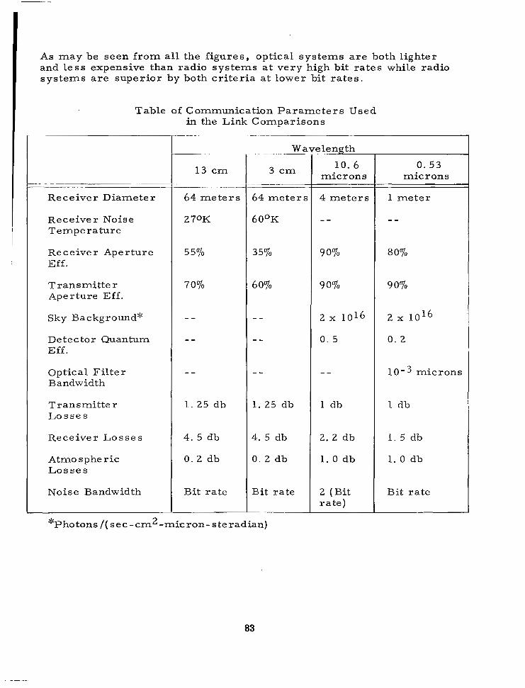
L
As m a y b e s e e n f r o m all t h e f i g u r e s , o p t i c a l s y s t e m s a r e b o t h l i g h t e r a n d l e s s e x p e n s i v e t h a n r a d i o s y s t e m s a t v e r y h i g h b i t r a t e s w h i l e r a d i o s y s t e m s a r e s u p e r i o r b y b o t h c r i t e r i a a t l o w e r b i t r a t e s .
Tab le of C o m m u n i c a t i o n P a r a m e t e r s U s e d in the L ink Compar isons
_" ~ "
R e c e i v e r D i a m e t e r
Rece ive r No i se T e m p e r a t u r e
R e c e i v e r A p e r t u r e Eff.
T r a n s m i t t e r Aper ture Ef f .
Sky Background':'
Detec tor Quantum Eff.
Op t i ca l F i l t e r Bandwidth
T r a n s m i t t e r L o s s e s
R e c e i v e r L o s s e s
Atmospher i c L o s s e s
Noise Bandwidth
1 3 c m ~~~. ~ ~-
6 4 m e t e r s
2 70K
"
1. 25 db
4. 5 db
0 . 2 db
B i t r a t e
. Wa
3 c m -
6 4 m e t e r s
60°K
3 5%
6 0%
"
"
"
1. 25 db
4. 5 db
0 . 2 db
Bi t ra te
? length
10. 6 m i c r o n s
4 m e t e r s
"
9 0%
9 0%
2 x 10¹⁶
0. 5
"
1 db
2 . 2 db
1. 0 db
2 (B i t r a t e )
0 . 5 3 m i c r o n s
1 m e t e r
"
8 0%
9 0%
2 x 10¹⁶
0. 2
1 0 - 3 m i c r o n s
1 db
1 . 5 db
1. 0 db
Bi t ra te
*Photons / ( sec-cm2-micron-steradian)
83

I 111 1 1 1 1 I11111 I I
Miashon Analysis and Methodology Methodology Examples and Conclusions
MICROWAVE AND LA-SER SYSTEMS COMPARED USING DESIGN CRITERIA
1
RS
(Sl6MlTOllOlSERATIO)(BITS PER SECOND1
Figure A.. Spaceborne Communications Systems Weight as a Function of Performance for Weight Optimized
Systems Using 1970 State of the Art and l o 8 K m Range
84
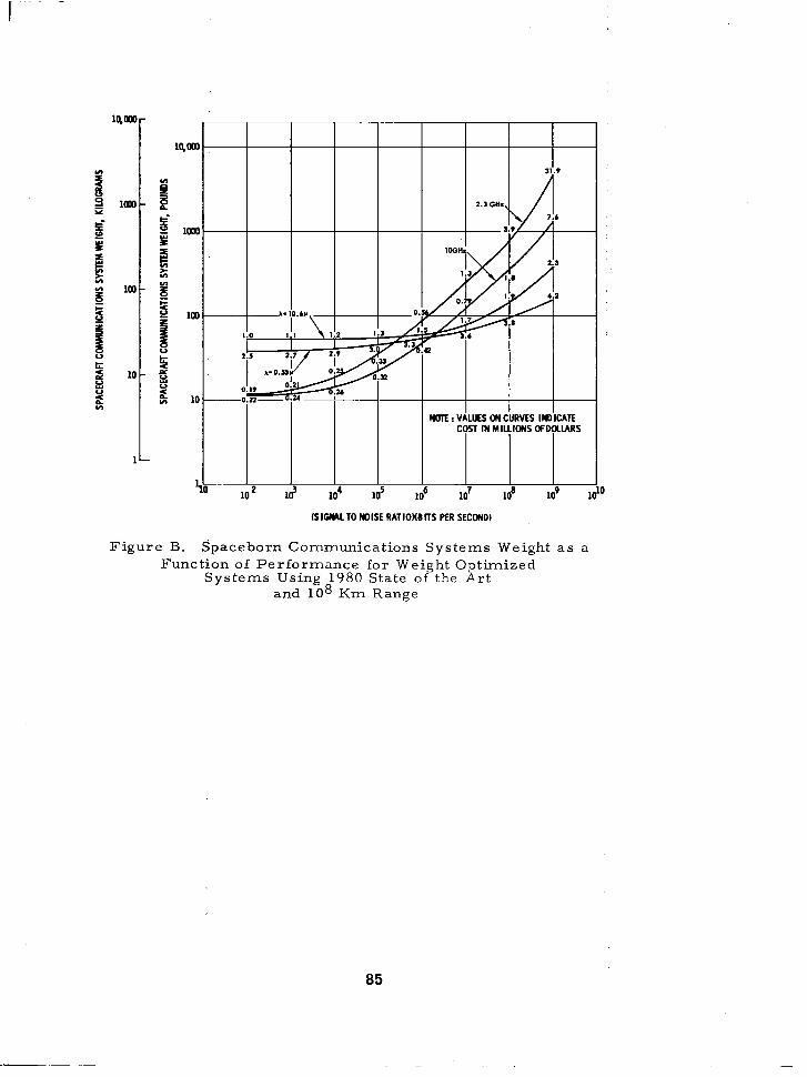
(SICWLTOWISE RATlOMBlTS PER SECOND)
Figure B. Spaceborn Communications Systems Weight a s a Function of Performance for Weight Optimized
Systems Using 1980 State of the Art and l o 8 Km Range
85

Mission Analysis and Methodology Me thodology Examples and Conclusions
MICROWAVE AND LASER SYSTEMS COMPARED USING DESIGN CRITERIA
tS I N 1 TO NOISE RATIOHE tTS PER SECOND1
P I
‘io dE
L lo9 .O
Figure C . Spaceborn Communications System Cost as a Function of Performance for Cos t Optimized
Systems using 970 State of the Art and 10 K m Range b
86

" .
T DTE : VALUES MIGHT ON IN 1 I
1 10'
ISIGMLTO WISE RATIO)(IITS PER SECOND)
F i g u r e D. Spaceborn Communica t ions Sys t em Cos t a s a Func t ion of P e r f o r m a n c e for C o s t O p t i m i z e d
Sys t ems u s ing 1980 Sta te of the Art and 108 K m Range
87

PART 2 SYSTEM THEORY
Section Page
Introduction . . . . . . . . . . . . . . . . . . . . . . . . . . . . . . . . . . . . . . . . . . . . . . . . . . . . . . . 90
Summary . . . . . . . . . . . . . . . . . . . . . . . . . . . . . . . . . . . . . . . . . . . . . . . . . . . . . . . . . 92
Detection Noise Analysis . . . . . . . . . . . . . . . . . . . . . . . . . . . . . . . . . . . . . . . . . . . . . . . . 94
Optical Detection . . . . . . . . . . . . . . . . . . . . . . . . . . . . . . . . . . . . . . . . . . . . . . . . . . . 110
Modulation Methods . . . . . . . . . . . . . . . . . . . . . . . . . . . . . . . . . . . . . . . . . . . . . . . . . . 136
Communication Coding . . . . . . . . . . . . . . . . . . . . . . . . . . . . . . . . . . . . . . . . . . . . . . . . 166
Telemetry Communications . . . . . . . . . . . . . . . . . . . . . . . . . . . . . . . . . . . . . . . . . . . . . . 172
89
System Theory
INTRODUCTION
Systems theory includes noise analy.sis, modulation and demodulation techniques.
Systems theory is concerned with information transmission for space communications. Theory is given for both radio and optical communica- tions. Optical communications is emphasized since it is relatively new and not as well documented in texts as is radio communications.
Systems theory is divided into five sections which are briefly introduced below.
Detection Noise Analvsis
In any sensing device there are certain random-interfering signals which must be considered. These noise signals include thermal effects, atmospheric effects, signal effects and background effects. These sev- eral topics are documented to show the relative importance of these interfering signals.
Optical Detection
Three types of optical detection are examined, direct detection, hetero- dyne detection and homodyne detection. Equations describing the per- formance of each are given.
Modulation Methods
Various modulation methods are described which are suitable for radio and optical systems. Relative performance and implementation com- plexity are indicated.
Telemetry Communications
Multi channel analog telemetry equations are derived and degradation caused by filtering is considered.
Communications Codine
The benefits which are possible using data compression is given. A l s o included is the cost in data transmission time due to synchronizing signals.
90

System Theory
SUMMARY
Systems theory provides the necessary equations to describe communications performance for a var ie ty of hardware implementations.
The.System theory documents the basic equations which describe modula- tion and demodulation implementations. The performance of these implementations is considered in the presence of various types of noise contributions.
In practice many optical and radio communications systems have been constructed and the theoretical performance compared to experimental measurements. The correlation has been good with small degradation allowed for hardware imperfections. It is not practical therefore to describe one type of implementation as "better than" another without listing the all conditions which are required to describe the theoretical performance. Instead the reader may select his own parameter values and compare performance as predicted by the equations in the text.
92

SYSTEM THEORY
Optical Detection Noise Analysis
Page Optical Detection Methods . . . . . . . . . . . . . . . . . . . . . . . . . . . . . . . . . . . . . . . . . . . . . . . 94
Thermal Noise . . . . . . . . . . . . . . . . . . . . . . . . . . . . . . . . . . . . . . . . . . . . . . . . . . . . . . . 98
Flicker Noise. Current Noise. and Dark-Current Shot Noise . . . . . . . . . . . . . . . . . . . . . . . . . . . . 100
Photon Fluctuation. Shot. and Generation-Recombination Noise . . . . . . . . . . . . . . . . . . . . . . . 102
Background Radiation Noise. Radiation Fluctuation Noise. and Phase Noise . . . . . . . . . . . . . . . . . . 106
Optical Detection Noise . . . . . . . . . . . . . . . . . . . . . . . . . . . . . . . . . . . . . . . . . . . . . . . . 108
93
" .
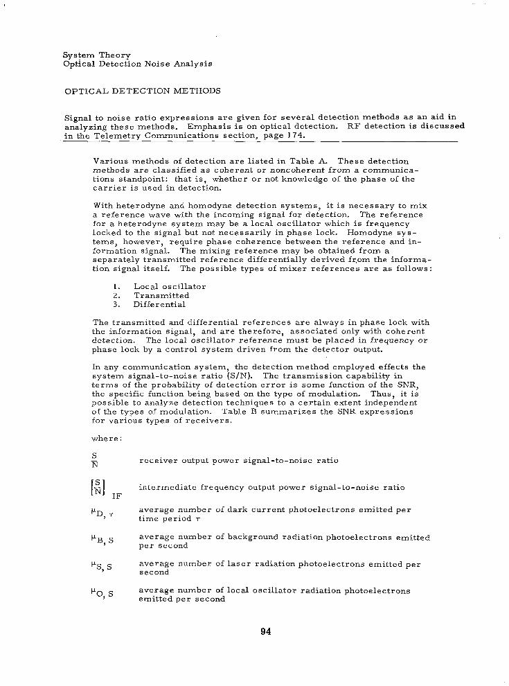
System -Theory Optical Detection Noise Analysis
OPTICAL DETECTION METHODS
Signal to noise ratio expressions are given for several detection methods as an aid in analyzing these methods. Emphasis is on optical detection. RF detection is discussed in the Telemetrv Communications section, page 174.
Various methods of detection are l isted in Table A. These detection methods are classified as coherent or noncoherent from a communica- tions standpoint: that is, whether or not knowledge of the phase of the c a r r i e r is used in detection.
With heterodyne and homodyne detection systems, it is necessary to mix a reference wave with the incoming signal for detection. The reference for a heterodyne system may be a local oscillator which is frequency locked to the signal but not necessarily in phase lock. Homodyne sys- tems, however, require phase coherence between the reference and in- formation signal. The mixing reference may be obtained from a separately transmitted reference differentially derived fr ,om the informa- tion signal itself. The possible types of mixe r r e f e rences a r e as follows:
1. Local oscillator 2. Transmit ted 3. Differential
The transmitted and differential references are always in phase lock with the information signal, and are therefore, associated only with coherent detection. The local oscillator reference must be placed in frequency or phase lock by a control system driven from the detector output.
In any communication system, the detection method employed effects the system signal-to-noise ratio (S /N) . The transmission capabili ty in t e r m s of the probability of detect ion error is some function of the SNR, the specific function being based on the type of modulation. Thus, it is possible to analyze detection techniques to a certain extent independent of the types of modulation. Table B summarizes the SNR expressions for various type.s of rece ivers .
where :
S N -
1 4 IF IJ.D, T
IJ.B, S
FS, s
Po, s
receiver output power signal-to-noise ratio
intermediate frequency output power signal-to-noise ratio
average number of dark current photoelectrons emitted per t ime period T
average number of background radiation photoelectrons emitted per second
average number of laser radiation photoelectrons emitted per second
average number of local oscillator radiation photoelectrons emitted per second
94

Table A. Optical Detection Techniques
I -~
Noncoherent
Heterodyne Homodyne Direct detection
Coherent -
Table B. Optical Detection Signal-to-Noise Ratio Expressions
Detec t ion Method
D i r e c t d e t e c t i o n ( a n a l o g t r a n s m l s s i o n )
~. ~
~~
D i r r c t d e t e c t i o n ( d i g i t a l t r a n s m i s s i o n )
Het t , rodyn<, dc . tc .c t~on ( d i g i t a l t r a n s m i s s i o n )
H o m o d y n e d e t e c t i o n ( a n a l o g t r a n s m i s s i o n )
H o m o d y n e d e t e c t i o n ( d i g i t a l t r a n s m i s s i o n )
"0, B l a r g c
E x p r e s s i o n
2
2
"S, E [;IIF = -
R B
S 2 u o , S " S , s = (US,SuO, S ' U B , S ' UD, S ) Bo
95
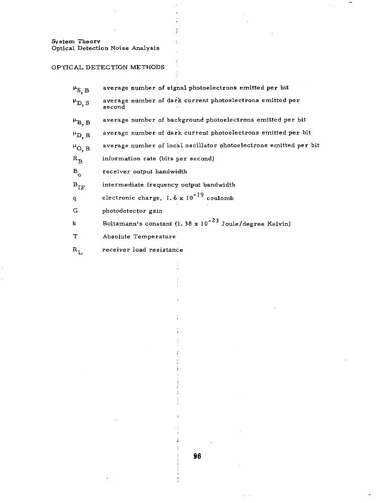
System Theorv Optical Detection Noise Analysis
OPTICAL DETECTION METHODS
' S , B
'D, S
'B, B
'I), B
'0 , B
RB
BO
BIF
q
G
k
T
RL
average number of signal photoelectrons emitted per bit
average number of dark current photoelectrons emitted per second
average number of background photoelectrons emitted per bit
average number of dark current photoelectrons emitted per bit
average number of loci1 oscil lator photoelectrons emitted per bit
information rate (bits per second)
receiver output bandwidth
intermediate frequency output bandwidth
electronic charge, 1. 6jx coulomb
photodetector gain
Boltzmann's constant (1. 38 x 10 - 2 3 Joule/degree Kelvin)
Absolute Temperature
receiver load resistance


System Theory Optical Detection Noise Analysis
THERMAL NOISE
The re la t ionship for thermal noise is defined and thermal noise is related to a s imple RC circuit.
Thermal or Johnson noise is caused by thermal fluctuations of e lectrons in a resistor. Consider a “noisy“ resistor, R, connected in parallel with a capacitance, C. In a practical detector, R may be the internal resistance of the detector or the load resistor, and C the detector shunt capacitance. The average energy stored in the capacitor in equilibrium may be equated to the thermodynamic energy of the system. Thus,
1 /2 C v2 = 1 / 2 k T -
where - v2 = mean square voltage across resistor
k = Boltzmann’s constant, 1. 38047 X watts f s e c - 0 K
T = res i s tor t empera ture
The thermal noise power is then
where the detector bandwidth is defined to be the reciprocal of the resistor-capacitor t ime constant.
The corresponding thermal noise power spectral density (two-sided) is
GT = 2 kTRL ( 3 )
This is the power spectral density of a noisy resistor connected to any detector filter network. If the detector network were an ideal (but physically unrealizable) bandpass network over a band between - f 2 to - f l and f l to f2, then the thermal noise power would be NT = 4kTAf where Af f 2 - f l . This leads to the treatment of thermal noise as being characterized by an open circuit rms voltage of
1 / 2
= (4k TR A f ) 1 / 2

and its rms current equivalent
lk2
[i: (Afl] = ( 4kT R Af )
in series or parallel, respectively, with a non-noisy resistor R. Care must be taken in the application of these equations since Af is, in general, not the bandwidth of the detector, but simply a frequency interval over which the thermal noise spectrum is flat. As an example of the application of these equations consider the thermal noise current source shunted by a capacitor as shown in the Figure. The total thermal noise power is the integral over all positive frequencies of the product of the mean square thermal noise current and the real part of the imped- ance of the RC parallel combination. Thus,
co 4k T R NT = [ T I [ ~ (2.rr RCf)2] df = -~ = kTB
kT RC
where the detector bandwidth is defined as in Equation (2).
( a 1 VOLTAQE SOURCE
THERMAL NOISE
CURRENT QENERATOR NOISE
RESISTOR
(b1 CURRENT SOURCE
Photodetector with Capacitor Filter Thermal Noise Model
99

System Theory Optical Detection Noise Analysis
FLICKER NOISE, CURRENT NOISE, AND DARK-CURRENT SHOT NOISE
Power spectrum. re la t ionships are presented for f l icker noise , current noise , and shot noise.
Flicker Noise
Fluctuations in the emission from a given point on a photoemissive surface creates f l icker noise. The spectrum of this noise is inversely proportional to frequency to less than 1 Hz and to the square of the average photocurrent. Thus,
Current Noise
Semiconductor devices carrying a steady current exhibit a cur ren t o r l/f noise which has a one-sided spectrum proportional to inverse fre- quency to below 1 Hz and to the square of the average detector current. Thus,
I2 GC ( f ) 3 - f
Trapping of charge car r ie rs near the sur face of mater ia l is believed responsible for the noise.
the s.emiconductor
Dark 'Current Shot Noise
A small current will flow in the absence of any external photoexcitation in a photoemissive or photovoltaic detector due to thermal emission, field emission, and current leakage within the detector. Experimental evidence indicates that dark current electron emissions from a cathode are time independent and obey Poisson statistics. The probability that the number of electrons emitted in a t ime period T is exactly an integer k is
(pD, T Ik exp {-pD P ( V D = k ) = k!
where
-r= - - IDT - average number of dark cur ren t 9
100

! ”.. . . .
I
e lectrons re leased by detector in T ; and ID = average detect+ dark current. These k electrons emitted at random t imes in T each car ry a unit electronic charge q and produce a total current I 1
!
k i (t) = 1 Gq6 (t - tn) for - 5 t 5 - ’
T T I
n=l 2 : I I
where d ( t - tn) is the unit impulse occurring at t ime tn and 6 is the post detector current gain.
In order to determine the power spectral density of the darkjcurrent fluctuations the autocorrelation function of iD(t) must be found. The Fourier t ransform of the autocorrelation yields the noise power spectral density
!
!
G ( f ) = G ID t G21D2 6 ( f ) 2
ID 9
I
i The noise power spectral density due to dark current emissipns is thus composed of a flat spectrum (GH (f) = qID) and a dc component. The total noise power, NHD, due to actuations about the mean over a band- width Bo a t a resist ive load RL is
N = 2 G I B RL 2
HD 9 D 0
This expression is called the Schottky shot noise formula. 4 s the dark current electrons move from the cathode to the anode, the npise spec- trum will be modified due to electron transit time effects. The resulting power spectrum is
I
where T~ is the electron transit t ime. In most detectors T~ i s small with respect to the reciprocal detector filter bandwidth, and:the electron transit t ime effect is negligible.
I
101
Svstem Theorv Optical Detection Noise Analysis
PHOTON FLUCTUATION, SHOT, AND GENERATION - RECOMBINATION NOISE
Shot noise is described and the spectral density from shot noise for photoemissive, photoconductive and photovoltaic detectors due to shot noise are given.
In all types of photodetectors, fluctuations in the arrival time of photons cause noise fluctuations in the detector current. The random arrival of k photons from a general radiative source may be described by
Taking the autocorrelation of MR ,(t) and the Fourier transform of M (t) yields a spectral density’of the photon fluctuations.
R, “
where E(WR) and E(WR ) are the first and second moments of the dis- tribution P ( W R = k) of the number of photon arrivals in T.
The number of photon arrivals due to background radiation (reflected sunlight, stars, etc. ) obeys Bose-Einstein statistics.
2
P ( W B = k) = [ Mg, T I k
[1 MB, T ]
where MB, = average number of background photon arrivals in time period T. The variance in the number of photon a r r iva l s i s1
1 Hodara, H, , “Statistics of Thermal and Laser Radiation, ’ ’ Proceedings of the IEEE, 2, No. 7, pp. 696-704, 1965.
102

where Ah/A is the ratio of the radiation coherence area to the detector area and B o ? B ~ is the ratio of the detector bandwidth to the coherence bandwidth. (Note: BB E 112- r~ where TC is the coherence time of the radiation. ) For background radiation, Ah/AD < 10-3 and BB =: 101 2 Hz. Thus, the second term of the variance expression is negligible. Since the mean of the Bose-Einstein distribution is MB the spectral density of the background photon fluctuations may be writ!ten as the average number of background photon arrivals per second [M = M / T I a s B, S B, T
( f ) = M + M 6 ( f ) 2
GMB, S B, s B, s
The statist ics of the number of photon ar r iva ls f rom a laser for var ious operating conditions is not presently well known. However, if the laser is assumed to be a purely monochromatic, single mode source, the l a s e r photon fluctuations may be described by a Poisson distribution. Thus,
where M = average number of l a s e r photon a r r iva l s T. s,
in t ime period
The spectral density of the laser photon fluctuations in terms of the average number of l a s e r photon arrivals per second [M = M / T I i s s, s,
In a photoemissive detector each arriving photon liberates an average of p g s = ? M B s and ps s = rlMs s electrons due to background and l a se r ' r ad ia t ion ahe re rl i z the deteztor quantum efficiency. While in photovoltaic and photoconductive detectors:;: the arriving photons create p~ s and ps s hole-electron pairs which create an electron current floh. Thus,' photon fluctuations at the input of a detector will produce photoelectron fluctuations at the output. The spectral densities of the electron emissions are then
.& 'The following statements to be made for photoconductive detectors apply also for photoelectromagnetic detectors since their physical mechanisms are s imilar .
103
I
I I I
System The.ory Optical Detection Noike Analysis
PHOTON FLUCTUATZON, SHOT, .AND, GENERAT1,ON - RECOMBINATION NOISE . . . . . . . . . . . . . . . . . . . . . . . . . . . , . . . . . . . . . . . . . . . . . . . . . . . . . . . . . . . . . . . . . . . . . . . . . . . . . . . . . -... ^ < .
. . . . . . . . . .> ....., .- L
and I
Since each photoelectron carries a unit charge, the power spectral densit ies of the detector currents about the average signal and back- ground current:s are
I
and
!
The noise power spectra
GHS = G 2 q Is
(photoemissive detector)
GHB = G 2 q IB
r l densi t ies are of the same form as the E noise power sp:ect;al densi t ies due to dark current , and are a lso referred to as ,shot noise.
!
;hot
In a photocond$ctive detector the simultaneous generation and recom- bination processes result in electron f luctuations twice as la rge as the photon fluctuations. The resulting noise power spectral densities about the mean detec' tor currents are
I G ( f ) = 2 G q Is 2
GS
and (photoconductive detector) !
This noise spebtrum is called generation-recombination noise by many authors, and simply shot noise by others. Lattice vibrations in the photoconductivk material will cause a modification of the basic generation-rec,ombination noise spectrum. The modification can be found by multiplying the G-R noise spectral density by the square of the absolute value 'of the impulse response of the lattice variations.
104
. . ......... .- ...... - .............

Thi s transfer function i s deDendent uDon the fracti onal ioniz material and whether the material is-intrinsic or extrinsic.
ation of the Jamieson,
e t al. , gives the G-R noise power spectral densities for these cases. . In most situations the lattice time constants are short with respect to the reciprocal detector f i l ter bandwidth, and the additional complexity is not warranted.
The recombination lifetimes in a photovoltaic detector are so short that the recombination process does not produce significant fluctuations. The expressions for $he photon fluctuation noise power spectral densities for a photovoltaic detector are then the same as the expressions for a photo- emissive detector.
G (f) = G q Is 2
GS
(photovoltaic detector)
LJarnieson, J .A. , etal., Infrared Physics and Engineering, McGraw-Hill, 1963.
105

System Theory Optical Detection Noise Analysis
BACKGROUND RADIATION NOISE, RADIATION FLUCTUATION NOISE, AND PHASE NOISE
The relative importance of background radiation noise, intensity noise, and phase noise is given.
. "" .
Background Radiation Noise
An optical direct detection receiver produces a detector current propor- tional to the instantaneous radiation intensity at the input to the receiver regard less of the frequency of the radiation passing through the optical input filter. Thus, i f the direct detection receiver is subject to a con- stant intensity background radiation, the only effect will be to ra ise the dc level of the detector output which does not affect the detection process.
In an optical heterodyne or homodyne receiver the constant intensity background radiation may mix with the receiver local oscil lator to pro- duce noise in the I F bandpass filter or output filter. The degree of mixing is proportional to the coherence of the background radiation. In general very little mixing occurs, and background radiation noise is negligible.
A radio frequency receiver responds to the electric field of the back- ground radiation. Mixing of the background radiation with itself and with a local oscillator will occur in nonlinear radio detectors producing appreciable background radiation noise.
Radiation Intensitv Fluctuation Noise
Random variations in the intensity of radiation causes noise fluctuations in the detector current. Variations in the background intensity are due to natural pulsations of the solar source or stars. Lasers suitable for communications generally are intensity stabilized, and therefore are not a ser ious source of radiation intensity fluctuations in themselves. However, all radiation passing through the atmosphere is subject to intensity variations due to the statistically changing atmospheric t ransmissivi ty .
A f i rs t order analysis of intensity fluctuations describes the fluctuations by some average percentage of intensity modulation of the source over a given frequency range. As an example, narrow-band background radia- tion intensity fluctuations may be described by an intensity fluctuation noise power of
N = M: G2 IB 2 RL =B
where
RL = Load resistor
G = Photodetector gain
IB = Current due to background photoelectrons
MF = intensity fluctuation modulation index (MF 5 1)
106

For typical background radiation levels MF must be less than 10 percent if the intensity fluctuation noise power is to be less than shot noise due to the background radiation.
Phase Noise
In a heterodyne or homodyne optical receiver in which optical mixing occurs, the l ine or spectral shape of the transmitting and local oscillator lasers becomes significant because the laser l ines are essentially shifted intact to a lower radio frequency called an intermediate frequency (IF). With a direct detection receiver consisting of a photodetector followed by a filter, laser line shape is not a consideration since the photodetector cannot differentiate between narrow-band optical frequencies. The spec- t r a l width at the IF becomes a problem i f frequency or phase detection is employed since the line width represents a phase uncertainty. With any type of optical mixing some form of phase or frequency detection is necessary in order to frequency or phase lock the laser carrier to the local oscillator, hence the phase uncertainty or phase noise is a problem even for an intensity modulation laser communication system.
The analysis of the effect of phase noise on a laser communication system is complicated by spectral variations of the laser radiation due to the atmosphere. The general approach is to determine the spectral shape of the I F signal and its statistical variations. The standard techniques of analysis developed for phase lock loops are then applicable.
107

System Theory ’
Gptical Detection Noise Analysis I
OPTICAL DETECTION NOISE
The spectrum relationships of various types of noise found in communications systems a r e given.
Detection Noise
Noise in the detection process of a communication system arises from radiation entering the communications receiver and internally generated noise. The major types of detection noise are l isted bel.ow:
Internal Noise
Thermal noise
Flicker noise
Current noise
Dark current shot noise
External Noise
Photon fluctuation shot and generation-recombination noise
Background radiation noise
Radiation intensity fluctuation noise
Phase noise
The Section on Detectors in Volume I11 contains details on these noise sources and their relationship to the physical parameters of the detectors. The following present an analysis of spec t ra of the noise sources.
Summary of Detection Noise Source
The Table lists the noise power spectral densities of the major detection noise sources. Flicker noise and current noise are low frequency phenomena, and their effects can be avoided by restricting the informa- tion signal bandwidth to above a low frequency cutoff of from 10 to 100 He o r by placing the information on a radio frequency subcarrier. The same techniques often negate the effects of intensity fluctuations of incident radiation on the detector.
The shot and generation-recombination (G-R) noise spectra due to dark current, background radiation, and laser radiation add to the detector output to produce a total shot or G-R noise power spectrum of
GH(f) = G qI (photoemissive detector)
G (f) = G qI (photovoltaic detector)
GG(f) = 2G qI (photoconductive detector)
L
2 G
2
108
whe r e
, , . I = total average detector current
GH(f) = shot noise power spectral density
G (f) = generation-recombination noise power spectral density G
q = electronic charge
Thermal noise is a universal type of noise found in all detection systems, and is usually the limiting noise source for semiconductors and photo- emissive detectors without secondary gain mechanisms. Secondary electron multiplication in a photomultiplier tube usually makes the detector shot noise limited. The dominance condition is that the shot noise be greater than the thermal noise power, or
2G qI Bo R L > k T Bo 2
The current gain required for shot noise limited operation is thus
where
G = photodetector gain
Bo = receiver output bandwidth
RL = receiver load resistance
k = Boltzmann's constant
T = Temperature
where
R = Resistance
aF = proportionality constant
aC = proportionality constant
I,, = average detector dark current
f = frequency
109

Power Spectral Densities of Major Sources of Optical Detection Noise
T h e r m a l n o i s e
F l i c k e r n o i s e ( p h o t o e m i s s i v e d e t e c t o r )
Curren t no ise (photovol ta ic and photo- conduc t ive de t ec to r s )
D a r k c u r r e n t s h o t n o i s e ( p h o t o e m i s s i v e and pho tovo l t a i c de t ec to r s )
Photon f luctuat ion shot noise (photo- e m i s s i v e d e t e c t o r )
Photon f luc tua t ion genera t ion- recombina t ion no ise (photovol ta ic de t ec to r )
Photon f luc tua t ion genera t ion- recombina t ion no ise (photoconduct ive de t ec to r )
E x p r e s s i o n ~~ . . ~ - . . .
~~
2 k T R
'FG f 2 I2
2 12 a c G f
G2 ql
G2 qI
2G qI 2
109a

System Theory Optical Detection
OPTICAL DETECTION STATISTICS
By assuming the optical statistics to be Poisson, relationships are derived which relate required threshold to signal, dark current noise, and background noise.
The statistical distributions of laser and background radiation photons at the input of a photodetector are complex functions, not necessarily time stationary. Mandel has shown, however, for low intensities the laser and background statistics may be assumed Poisson. Thus, let the proba- bility distributions of laser and background photon counts be
P ( W = k) = B k!
where
W is the number of background radiation photons at detector in B time period T
W is the number of laser radiation photons at detector in t ime S ' period T
M is the average number of background radiation photon arrivals B, per t ime period T
s, I- time period T M is the average number of laser radiation photon arrivals per
k is an.integer
Since the photon counts are related to the photoelectrons counts by the quantum efficiency, '1, the output distributions of photoelectrons is a l so Poisson. The probability distributions of photoelectron counts due to l a se r and background radiation are
'Mandel, L., "Fluctuations of Light Beams, '' in Progress in Optics, John Wiley and Sons, 1963.
110

"
where
ps, E MS, T, and p M B, T B,
V is the number of background radiation photoelectrons emitted B in t ime per iod r
Vs is the number of laser radiation photoelectrons emitted in t ime per iod T
. . , .
In addition to the laser' and background emissions, the detector will a l s o release electrons due to the detector dark cur'rent. The probability dis- tributions of the dark current emission is also Poisson.
where
I T
% T - 9 " , and ID = average detector dark current.
VD = number of dark current photoelectrons emitted in t ime period T
The three emission processes are independent, and hence, the probabili ty distributions of photoelectrons due to the simultaneous presence of l a se r and background radiation and dark current are Poisson distributions whose means are the sums of the means of the constituent distributions. The photoelectron count distribution for no laser signal present is
where
pN, T = pB, T ' FD, T
VN = Number of noise radiation photoelectrons emitted in time period T.
The corresponding distribution when the laser signal is present is
e
111

System Theory Optical Detection
OPTICAL DETECTION STATISTICS
where
VSN = Number of signal and noise radiation photoelectrons emitted in t ime period T.
In many communication systems the absence or presence of a laser s ig- nal is determined by comparing the received photoelectron count with a predetermined threshold level. The thres old level is determined from the likelihood ratio test of decision theory? The likelihood ratio test states that a signal is present i f
where
A(k) = likelihood ratio
P (S#O) = a priori probabili ty that signal is not present
At the threshold value kt of k,
k .
Since the likelihood ratio is a monotonic function of the threshold value, the expression may be inverted to yield
The output of a photodetector is an integer number of photoelectrons, and hence, the actual threshold Nt chosen should be the greatest integer value of kt. The Figures show the likelihood ratio test threshold as a function of the signal and noise photoelectron counts for PCM and PPM threshold detection.
2Reiffen, B. and Sherman, H., "An Optimum Demodulator for Poisson Processes: Photon Source Detectors, " Proceedings of the IEEE, 5 3 , No. 10, p. 1660, October 1965.
-
112

Likelihood Ratio Test Threshold for
PCMIIM Laser Communication
System
PPM/IM Likelihood Ratio Test Threshold
113


SYSTEM THEORY
Optical Detection
. . . . . ....
..
. . . . .... . . . . ". 1
Optical Direct Detection . . . . . . . . . . . . . . . . . . . . . . . . . . . . . . . . . . . . . . . . . . . . . . . 116
Optical Heterodyne Detection . . . . . . . . . . . . . . . . . . . . . . . . . . . . . . . . . . . . . . . . . . . . 122
Optical Homodyne Detection . . . . . . . . . . . . . . . . . . . . . . . . . . . . . . . . . . . . . . . . . . . . . 130
115

System Theory Optical Detection
. . __ ._. ". . "" -
OPTICAL DIRECT DETECTION
The signal to noise ratio is developed for the general case and then modified for a variety of spec ia l cases of optical direct detection.
The operation of an optical direct detection receiver is illustrated by Fig- u re A. The current produced by the background noise and the signal itself combine with the dark current to produce shot noise in the detector. The composite signal and shot noise current is multiplied, filtered, and combined with thermal noise in the load. The detector multiplication factor may be unity to encompass devices without photomultiplication.
A photodetector is essentially an intensity to current converter in the wave sense or a photon to electron converter in the quantum sense. Let
M = average number of signal photons impinging on photodetector '7 per second
ps, = average number of signal photoelectrons released by photo- detector per second
= detector quantum efficiency (rl < 1 )
h = Planck's constant (6. 624 x 10 joules-sec) -34
f = carr ier f requency
PC = car r ie r power at detector surface
Then the average signal photon count per second is equal to the ratio of the average signal power to the energy of a single photon at the carrier frequency.
NoteIn this and the following two topics only the principal noise sources- shot and thermal noise - are considered. For a photoconductive or photoelectromagnetic detector the shot noise power should be doubled.
116

A group of MS s photons striking the detector releases an average of ?Ms, s photoelkctrons. Thus,
ps, = q M (photon to electron converter) s,
Each photoelectron carries a charge of 1 .6 x coulombs to produce an average detector s ignal current of .
Is = qps, s Thus.
%PC
hfC
Is = qqMS, = - (intensity to current converter)
The signal power at the detector output consisting of a load resistance R is L
2 2 S = (GIS) RL - - ( Grlq hfc pc ) R L
where
G is the photomultiplication gain
RL is the load resistance
The average current at the output of the photodetector due to background radiation is
pB IB = - hfC
? q
where
PB is the power of the background radiation at the detector surface
The shot noise power as given by the Schottky formula is
NH = 2 qG2 I BoRL
where
B is trLc. receiver output bandwidth, I i i t he ave rage de t ec to r cu r ren t 0
1 = 1 + I + I D S B
117

System Theory Optical Detection
OPTICAL DIRECT DETECTION
and
ID = dark cur ren t
Then
NH = 2q B o G 2 ( x P C hfc txPB t ID h f C
The thermal noise power is
N T = k TBo
The signal-to-noise ratio is then
s - ’ - k T B o t 2qBoC2 (%PC +=PB f ID) RL h f C
For a detector with large postdetector gain the shot noise and back- ground noise are much larger than the thermal noise. Thus,
S N - ”
2q Bo (F p~ t X P B hfc t ID (no thermal noise)
The dark current of a detector can be made negligible by cooling the detector. Then
s - - 2 Bo hfc (PC tPB) (no dark current)
118

If the background noise input power is l a rge r power
than the carrier noise input
shot noise limited
If the carrier input power is larger than the background noise input power
"
N 2 Bohfc - (carrier shot noise l imited operation)
The complete optical communication system into which the direct detec- tion fits is shown in Figure B.
119

THERMAL NOISE - CARRIER PLUS BACKGROUND RADIATION
OPTICAL F I LTER
SIGNAL PLUS -
D,!:tl& SURFUX
b Lob0 ELECTRICAL CURRENT SHOT NOISE YULTIPLICATION FILTER -&
- t
MRK CURRENT
Figure A. Direct Detection Model
120

I
r------ 1 COMMUNICATION r-------- 1 I I I- -4 I I RANGE
I DRIVING SIGNAL, Pnf,
I MODULATOR
I
I
- DRIVER
SIGNAL, DIGITAL
2nfm
I CONVERTER: INCLUDES ANALOG-TO-DIGITAL
K M ENCODER
TRANSMITTER ANALOG SIGNAL, fm
SOUICE, SIGNAL
fm
I ELECTO-OPTICAL I SIGNAL
(PR)' CRYSTAL 2nfm DIGITAL-TO-ANALOG I 6 ) W T
M E R OSCILLATOR,
OR
s ' > ~ ~ ~ - ~ ~ (pg) I I , PHOTODETECTOR sirs_ INTEGRATE 6 DUMP,
CONVERTER, INCLUDES: SIGNAL* fm
b
fc PT
I - [ CIRCUITS 1 1 DECISION, DECODW AND LOW PASS FILTER
TRANSMITTER RECEIVER OPTICS,
TT OPTICS,
r R
RECEIVED
0 0 FIELD STOP A RE-COLLIMATING LENS
SPECTRAL FILTER (to filter out background rcdiation)
I QUARTER WAVE
i I I PLATE SIGNAL ANALYZER 1 (see enlargement)
RIGHT OR LEFT CIRCULARLY POLARIZED J
DETECTORS (photomultipliers) PLATE PRISM
SIGNAL ANALYZER ENLARGEMENT DIRECT DETECTION F€M/PL RECEIVER COMPONENTS (visible spectrum)
Figure B. Optical Digi ta l Communicat ion System Using Direct Detect ion

System Theory Optical Detection
OPTICAL HETERODYNE DETECTION
The signallto-noise ratio for an optical detection receiver is derived and compared with optical direct detection.
- ~ _ _
In a heterodyne detector, as shown in Figure A, the incoming carrier is mixed with a reference wave on a photodetector surface producing sum and difference frequencies. The difference frequency is then passed through an electrical filter to the load.
The principal advantages of heterodyne operation are the relative ease of amplification at an intermediate frequency, and the fact that the local oscillator power may be set to swamp out the thermal noise and shot noise caused by all other sources than the local oscil lator i tself .
Figure B illustrates the spatial combination of the carrier and local oscillator on the detector surface when the beams are misaligned by an angle 9 . Let
where p E mo/vx and vx is the local oscillator wave velocity along the detector surface. The carrier and local oscillator instantaneous amplitudes combine at the photodetector surface to yield an input nor- malized power to the detector of
[Ac cos (wet + + c ) + A. cos ( m o t t +o - px)I2
The resultant instantaneous carrier and local oscillator current at the photodetector output is the spatial integral of the light intensity over the detector surface.
+ 112 A," cos 2mct + 112 A," cos 2 ( m o t - p x ) dx I 122

where
'1 = quantum efficiency
g = electronic charge
h = Planck's constant
f c = car r ie r f requency
d = surface dimension
The average photodetector current due to the carrier and local oscillator is
Ip = 7 D (A: + A:) = D (PC t Po)
The intrinsic bandwidth limitations of the photodetectors provides a filter for the double frequency terms. Only the difference frequency will be passed by the I F fi l ter to give an instantaneous IF frequency current .
Performing the integration yields
s in (g) iF = D A A cos [(w, - wc) t t (+o c o - +&I
From Figure B
where
c = velocity of light
123
L.
System Theory Optical Detection
OPTICAL HETERODYNE DETECTION
and therefore,
w s in + 2.rr+ 0
P = = - X 0
where
X. = local oscillator wavelength
In order that signal phase cancellation due to misalignment be kept to 10 percent or less (pd/2) must be 0. 8 radian or less . Thus,
At a wavelength of cm and for a detector surface of 1 cm, $mus t be held to 10-4 radian or less. The spatial al ignment requirement can be minimized somewhat by focusing the signal beam to its diffraction l imited spot size on the detector surface which may be on the order of 0. 01 cm yielding an allowable misalignment angle of radlall. If such a procedure is followed the local oscillator beam must be focused or field stopped to the signal spot size to prevent additional shot noise due to the local oscillator.
Assuming perfect spatial al ignment, the average carrier power at the IF f i l t e r re fe renced to a unit resistance is
[SIIF = [GiF] = 2G D Po PC 2 2 2
where G is the net amplification.
The shot noise power at the output of the IF f i l t e r re fe r red to a unit res i s tance i s
where
1 = 1 + I + I P B D
Then
[NHIIF = 2G 2 q BIF(DPC t DPO t DPB t ID)
124

The SNR at the output of the IF f i l ter is
If the local oscillator power is large, all signal, background and dark current shot noise effects plus the thermal noise will be swamped out by the local oscillator shot noise. The S / N is then
Since the I F bandwidth BIF is at least twice as large as the baseband Bo, the SNR of a heterodyne receiver can at most equal the SNR of a d i rec t detection receiver for signal shot noise l imited operation. Second detec- tion must now be performed to obtain the information signal from the IF c a r r i e r . First consider that the electrical detector is a square law de- vice in which the I F output is squared. The output of the electrical square law detector is
At the output of the subsequent low pass filter the signal current is
G D A, A. 2
2 2 2 2
is = 2 2 = 2G D POPc
which yields an output current directly proportional to the input power.
The output power is
S = F R L = 4G D Po PC RL 4 4 2 2
125

System Theory Optical Detection
OPTICAL HETERODYNE DETECTION
The I F filter noise output when fed to the square law detector along with the signal will result in signal and noise cross product terms. I t may be assumed that the shot noise in the IF filter bandwidth, which has a flat spectrum, is generated by a narrow band Gaussian process. Then the analysis1 for a modulated sine wave plus Gaussian noise input to a square law detector will apply.
In this case the receiver output noise is related to the IF output noise by
The output signal-to-noise ratio is then
I
In the limit when the IF SNR is la rge
- 2 [,]IF - r s
and when the IF SNR is smal l
2
= [%]IF
Thus, square law second detection results in at least a 3 db reduction in SNR, and significantly degrades the receiver output i f the IF SNR is low.
For a low IF signal-to-noise ratio, synchronous second detection pro- duces better results. In a synchronous second detector the IF output is multiplied by a sine wave at the IF center frequency.
The output of the electrical synchronous detector is
GDAc A. GDAcAo iR iF cos w t = d COS (+o-+c) - sin 2 w d t s in (+ o c -+ )
‘Davenport, W. B., J r . and Root, W. L., An Introduction to the Theory of Random Signals and Noise, McGraw-Hill, 1958.
126

where
Wd wo - 0 C
At the output of the low pass the filter s ignal current is
to yield a signal power of
G D Ac A. 2 2 2 2 7 S = is RL = 2
4 cos (+o-+c) R L
= G D P P COS R L 2 2 2 s o
Assuming a uniform distribution of the phase angle (p -+ , the signal power is o c
s = - G2 D2 PC Po R L 2
The shot noise power in the output filter bandwidth is reduced by the rat io of the receiver output bandwidth to the I F bandwidth
Since BIF is ideally 2B0, the receiver output noise power is one half the I F output noise power.
Then the signal-to-noise ratio is
127

System Theory Optical Detection
OPTICAL HETERODYNE DETECTION
or
N 4hfc Bo (PC + Po + PB)
For Po l a rge
Synchronous second detection thus results in a SNR of one-half that obtained for a signal shot noise limited direct detection receiver.
128

- CARRIER PLUS BACKGROUND O-, RADIATION
OPTICAL PHOTO IF ELECTRICAL ELECTRICAL
FILTER DETECTOR FILTER OUTPUT * FILTER DETECTOR *
LOCAL OSCILLATOR
Figure A. Local Oscillator Reference Heterodyne Detection Model
\PHOTODETECTOR SURFACE
Figure B. Spatial Combination of Ca r r i e r and Local Oscillator
129
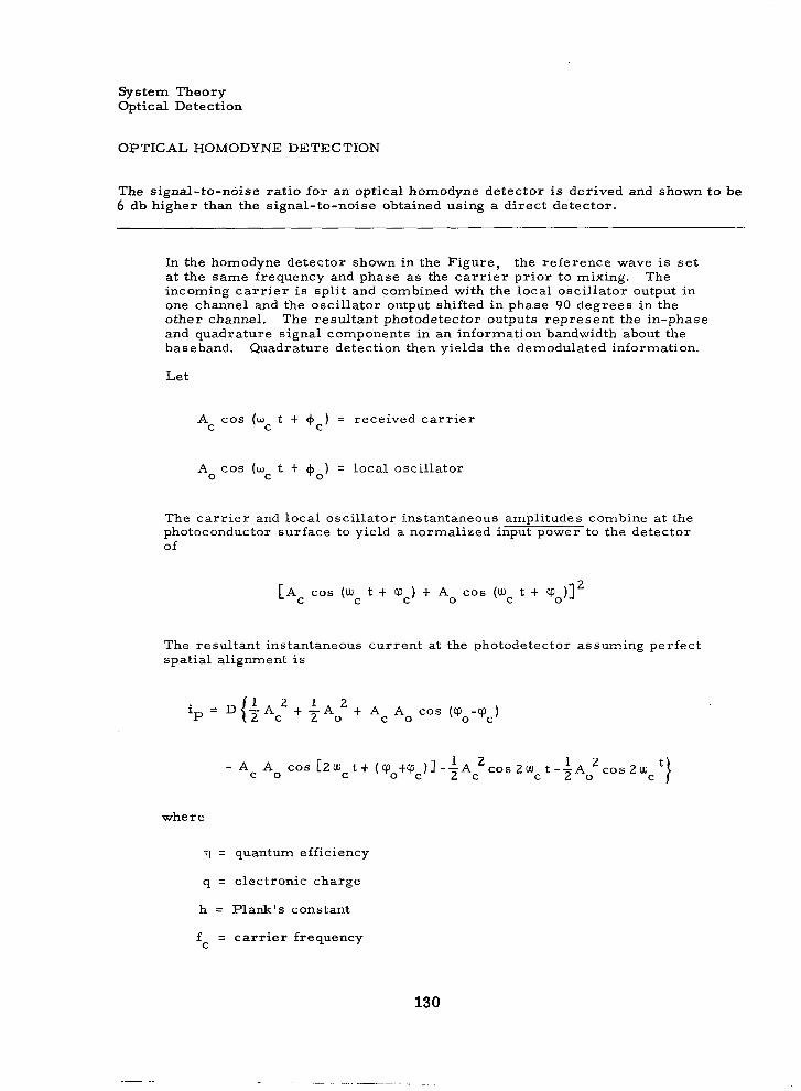
System Theory Optical Detection
OPTICAL HOMODYNE DETECTION
The signal-to-noise ratio for an optical homodyne detector is derived and shown to be 6 db higher than the signal-to-noise obtained using a direct detector.
In the homodyne detector shown in the Figure, the reference wave is set at the same frequency and phase as the carrier prior to mixing. The incoming carr ier is split and combined with the local oscillator output in one channel and the oscillator output shifted in phase 90 degrees in the other channel. The resultant photodetector outputs represent the in-phase and quadrature signal components in an information bandwidth about the baseband. Quadrature detection then yields the demodulated information.
Let
A COS (w t t + ) = rece ived car r ie r C C
A cos ( w t t I$ ) = local oscil lator 0 0
The carrier and local oscillator instantaneous amplitudes combine at the photoconductor surface to yield a normalized input power to the detector of
The resultant instantaneous current at the photodetector assuming perfect spatial alignment is
ip = .{+A: t -A 1 2 t Ac A. cos (cp -rp ) 2 0 o c
- Ac A. COS [2*ct t (ePoSePc)~-yAc 1 2 c o s Z ~ C t - ~ A ~ ~ ~ ~ 2 ~ 1
where
q = quantum efficiency
q = electronic charge
h = Plank's constant
f = carr ier f requency C
130
CARRIER PLUS BACKGROUND RADIATION
I
PHOTO DETECTOR
NO. 2
- ELECTRICAL
FILTER
-
~
DETECTOR PHOTO
NO. I
LOCAL
ELECTRICAL . QUADRATURE FILTER DETECTOR
w LOAD
Local Oscillator Reference Homodyne Detection Model
131

System Theory Optical Detection
OPTICAL HOMODYNE DETECTION
ip = instantaneous detector current due to carr ier and local oscillator
iH Y instantaneous homodyne receiver output current
is = instantaneous receiver output current
The intrinsic bandwidth limitation of the photodetector provides a filter for the double frequency terms to yield,
i H - - .{+A: ++A: t Ac A. C O S (qo-Cpc))
In a homodyne receiver the carrier and local oscil lator are phase locked so that +o = +c. The signal portion of the output is then
is = D Ac A.
and the signal power is
S = (G is)' RL = 4G D Po PC RL 2 2
where
G is the net.receiver gain
RL is the load resistance
The shot noise power neglecting dark current is
Thus the signal-to-noise is
132

If the .local oscillator power is large
s 2q = (strong local oscillator)
The signal-to-noise ratio for a homodyne receiver is therefore 6 db greater than the SNR for signal shot noise limited direct detection receiver.
133

111111.11.1 1 1 1 1

SYSTEM THEORY
Introduction . . . . . .
Modulation Methods
Page . . . . . . . . . . . . . . . . . . . . . . . . . . . . . . . . . . . . . . . . . . . . . 136
Type I Modulation Systems . . . . . . . . . . . . . . . . . . . . . . . . . . . . . . . . . . . . . . . . . . . . . . 138
Type I I Modulation Systems . . . . . . . . . . . . . . . . . . . . . . . . . . . . . . . . . . . . . . . . . . . . . 140
Type Ill Modulation Systems . . . . . . . . . . . . . . . . . . . . . . . . . . . . . . . . . . . . . . . . . . . . . . 142
Optical Pulse Code Intensity Modulation . . . . . . . . . . . . . . . . . . . . . . . . . . . . . . . . . . . . . . 146
Optical PCM Polarization Modulation . . . . . . . . . . . . . . . . . . . . . . . . . . . . . . . . . . . . . . . . 148
Optical PCM Frequency Modulation . . . . . . . . . . . . . . . . . . . . . . . . . . . . . . . . . . . . . . . . . 152
Optical PPM Intensity Modulation . . . . . . . . . . . . . . . . . . . . . . . . . . . . . . . . . . . . . . . . . . 154
Radio Amplitude, Frequency, and Pulse Code Modulation . . . . . . . . . . . . . . . . . . . . . . . . . . . . 156
Pseudo Random Noise Modulation for Radio Communications Systems . . . . . . . . . . . . . . . . . . . . 160
13 5

System Theory Modulation Methods
INTRODUCTION
Modulation methods are defined by the extent the data signal is modified before it is impressed upon the carrier.
Methods of modulation can be classified into three essential techniques. The first t ransforms a source signal waveform into a continuously vari- able modulation parameter. The second involves time sampling with continuous modulation parameters. The third is character ized by sampling time and allowing the source signal to take on only a d iscre te s e t of possible values. These three techniques are summarized in the Table.
Where :
AM
FM
IM
PAM
PIM
P P M
PDM
PCM
PCM/AM
PCM /IM
PCM / FM
PCM/PL
PCM/PM
amplitude modulation
frequency modulation
intensity modulation
pulse amplitude modulation
pulse intensity modulation
pulse position modulation
pulse duration modulation
pulse code modulation
PCM amplitude modulation
PCM intensity modulation
PCM frequency modulation
PCM polarization modulation
PCM phase modulation
136

T i m e
Laser Modulation Techniques
Modu la t ion pa rame te r (ampl i tude , f requency phase , po lar i ty , e tc . )
E x a m p l e s
Continuous
Continuous
FM, AM, IM
Type I1
Sampled
Continuous o r quanti2 ed
PAM, PIM, P P M , PDM
Type I11
Sampled
Quant ized and coded
P C M I A M P C M I P L PCM/'IM P C M I F M P C M I P M
137

System Theory Modulation Methods
TYPE I MODULATION SYSTEMS
Several Type I communication modulation methods are related to general expressions for the transmitted f ield vectors.
Communication systems utilizing Type I modulation techniques employ modulation which varies the parameters of the sinusoidal carrier wave- form. In considering the modulation methods, the condition that the carr ier waveform is spectrally isolated from the modulation waveform must be satisfied. The Type I modulation systems can be descr ibed by the orthogonal electric field vectors
where Fx(t), Fy(t), +x(t), and +y(t) are amplitude and phase functions of the modulating slgnal x(t) and the type of modulation. The conditions of this equation for various types of modulation are listed.
Amplitude Modulation Phase Modulation
+.Jt) = +y(t) = +, Fx(t) = F1, F (t) = F2 Y
Frequency Modulation
Polarization Modulation
4 q t ) = +y(t) = +c
x( t ) = tan
138

A radio frequency carrier can be amplitude, frequency, or phase modulated. At optical frequencies polarization modulation is possible as well as intensity, frequency, or phase modulation.
139
I

System Theory Modulation Methods
TYPE I1 MODULATION SYSTEMS
In Type I1 modulation systems, the modulation is imposed upon a pulsed carrier energy.
In t ime-sampled systems a sample from a signal source is used to modu- la te a carrier waveform so that at the receiving end of the communication link a sampled representation of the signal source may be reconstructed. For a band-limited information signal of bandwidth B, a signal sampled at a ra te of 2B samples per second can be faithfully reconstructed at the receiver . In practice, sampling rates higher than the theoretical mini- mum are often required because most signals are not truly band-limited.
Waveform parameters are available for Type I1 systems which cannot be applied to Type I systems. These parameters include the shaping of a t ransmission pulse in some manner or the var ia t ion of the t ime occurrence of a pulse. The commonly used systems of pulse modulation are listed below.
PAM - pulse amplitude modulation
PIM - pulse intensity modulation
PDM - pulse duration modulation
PPM - pulse position modulation
In radio or optical frequency Type I1 communication systems a burs t of the car r ie r is transmitted. The envelope of t he ca r r i e r fo rms a pulse, and it is the amplitude, duration, or position of this pulse envelope that carries the transmitted information.
In pulse intensity modulation, PIM, the signal keys the carrier on and off.
140

System Theory Modulation Methods
TYPE I11 MODULATION SYSTEMS
Probability of error re la t ionships are given for various PCM radio and optical communication systems.
In Type I11 modulation systems the signal parameter is quantized, and the signal is time sampled. A finite number of waveforms is used to represent each signal sample; the smallest number of waveforms is, of course , two. Modulation systems employing only two transmitter wave- forms are called pulse code modulation (PCM) systems. Systems em- ploying a large number of waveforms have found little application in communications to date but hold promise of improved performance over two level systems.
In theory the two transmitter waveforms of PCM could take any form. For optimum detection the waveforms should be the negative of each other or orthogonal. The usual forms of the t ransmit ted waveforms are rectangular pulses. PCM data can be conveyed by severa l means : a burst of the car r ie r of the absence of it -, intensity modulation, PCM/ IM; amplitude modulation, PCM/AM; a c a r r i e r of two possible frequen- c ies -, frequency shift keying, PCM/FM; a car r ie r wi th a 0- or 180- degree phase relationship - phase shift keying, PCM/PM; or a c a r r i e r of right- or left-hand polarization - polarization shift keying, PCM/PL.
Probability of detect ion error expressions are summarized in the Table .
PSN B
PSN P
PN'
pe
P' e
'N, B
'S, B
'N, P
' s , P
probability that signal plus noise photoelectron count equals or exceeds decision threshold during a bit period
probability that signal plus noise photoelectron count equals or exceeds decision threshold during a sample period
probability that noise photoelectron count equals or exceeds decision threshold during a bit period
probability that noise photoelectron count equals or exceeds decision threshold during a sample period
probability of bit detection error
probability of sample detect ion error
average number of noise photoelectrons emitted in a bit period
average number of signal photoelectrons emitted in a bit period
average number of noise photoelectrons emitted in a sample period
average number of signal photoelectrons emitted in a sample period
142

I
Probability of Error Expressions
R a d i o P C M l A M ( n o n c o h e r e n t d e t e r 1
- R a d i o P C M / A M ( c o h e r e n t detection)
O p t l c a l P C M l P L
( h e t e r o d y n e d e t e c t t c
( n o n c o h e r e n t d e t e c t
D e t e c t t o n Statistics
Pot s son "
Gauss ian
Cdusa ian
Poisson
G a u a s l a n
Ciausmian
w h e r e
k
k : k - N
w h e r e N I = g r e a t e s t i n t e r g e r value of k:
where K i s d e f i n e d by
143

System Theory Modulation Methods
TYPE I11 MODULATION SYSTEMS
S y s t e m
R a d i o P C M I F M ( c o h e r e n t d e r c c t l o n )
R a d i o P C M I A M ( c o h e r e n t d e t e c t i o n )
~ ~
Radio P C M I A M [ d ~ l l e r e n t ~ a l l y c o h e r e r ) i e t e c t l o n l
3 p t i c a l PI" t h r e s h o l d d e t e c t i o n )
D e t e r t l u n S c a t i s t t c s
G a u s s i d n
G a u s s i a n
G a u s s i a n
P o i s a o n
Pe = f [ I - c r f I;..-, ] 'E
P (1 - P,' ) L - l
[ I -31 + [ Lp,. ] [p& - 4 u h r r e
k
PN 1 (T ) e x p I-(+)[ 2 k = N I k !
4; = g r e a t e s t i n t e g e r v a l u e of k p T
L number of time positions
E Signal energy per bit
NO noise spectral density
[:I,, intermediate frequency output power signal-to-noise ratio
144


System Theory Modulation Methods
OPTICAL PULSE CODE INTENSITY MODULATION
Probability of bit .error for an intensity modulated optical carrier is derived and plotted as a function of signal and background photoelectrons.
In the optical PCM/IM system, signal photons are transmitted for a "one" bit and no signal photons are transmitted for a "zero" bit. Let
= probability that the signal plus noise photoelectron count PSN equals or exceeds decision threshold NT during a bit period.
PN = probability that the noise photoelectron count equals or B
exceeds decision threshold NT during a bit period.
Then, based upon Poisson detection statistics, the signal plus noise and noise detection probabilities are
where
= average number of signal photoelectrons emitted b y photodetector per bit period
pN'B photodetector per bit period. = average number of noise photoelectrons emitted by
The optimum threshold, N:, is the greatest integer value of the
ratio threshold, kT, where B likelihood
146

w h e r e
p = a p r io r i p robab i l i t y of t r ansmi t t i ng a "one" bit.
The probabi l i ty of a b i t e r r o r is then
-
P = [probabi l i ty tha t a "one." is t r a n s m i t t e d e 1 [ probabi l i ty tha t s igna l p lus no ise does no t
exceed t h re sho ld 1 I t [probabi l i ty tha t a "ze ro" is t r a n s m i t t e d
probabi l i ty tha t no ise equals o r exceeds th reshold 1 Thus ,
Fo r
1 p = - 2
[ S N -t e 2 B
P = - 1 - P
In t e r m s of the de tec t ion probabi l i t i es
#-
The Figure shows the probability of detection error as a function of the signal and noise photoelectron counts per bit period.
147
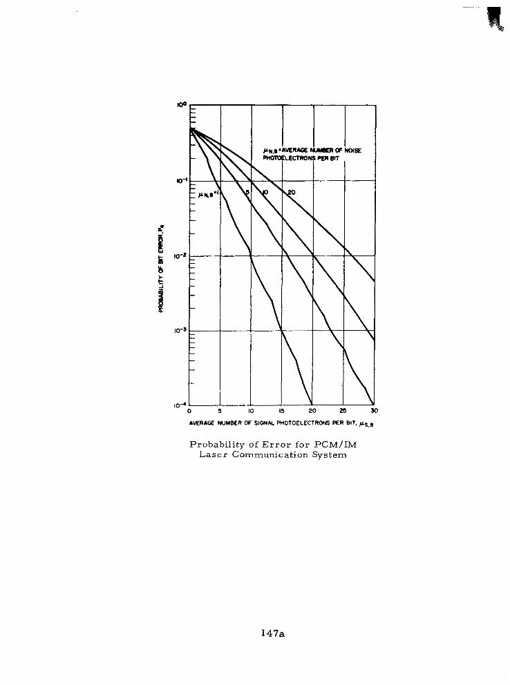
". . .
1 0 - 4 - 1 - L 0 5 IO IS 20 25 30
AVERAGE NUMBER OF SIGN& PHOTOELECTRONS PER BIT. p s , ~
Probability of E r r o r for PCM/IM Laser Communication System
147a

System Theory Modulation Methods
OPTICAL PCM POLARIZATION MODULATION
Probability of bit e r ro r fo r a polarization modulated optical carrier is derived and plotted as a function of signal and background photoelectrons.
In the optical PCM/PL system, the carrier is transmitted in right circu- lar polarization to represent a "one" bit, and in left circular polarization to represent a "zero" bit. The probability of detection error may now be derived for the difference detection model illustrated in Figure A. Let
X = right detector output
Y = left detector
z = x - Y Assuming that the laser carrier is right circularly polarized, a detection e r r o r will occur when Y > X with probability 1 , or when Z = 0 with probability of 1 / 2 . By symmetry of the channels the probability of e r r o r is
m
p = 1 + - P ( Z = O ) - 1 e 2 c
j=O P ( Z = j )
The term P (Z = j ) may be determined by summing over the joint dis- tribution of the output channel yielding a difference, Z = j .
where based upon Poisson detection statistics, the detection probabilities of the X and Y channels are
i !
148
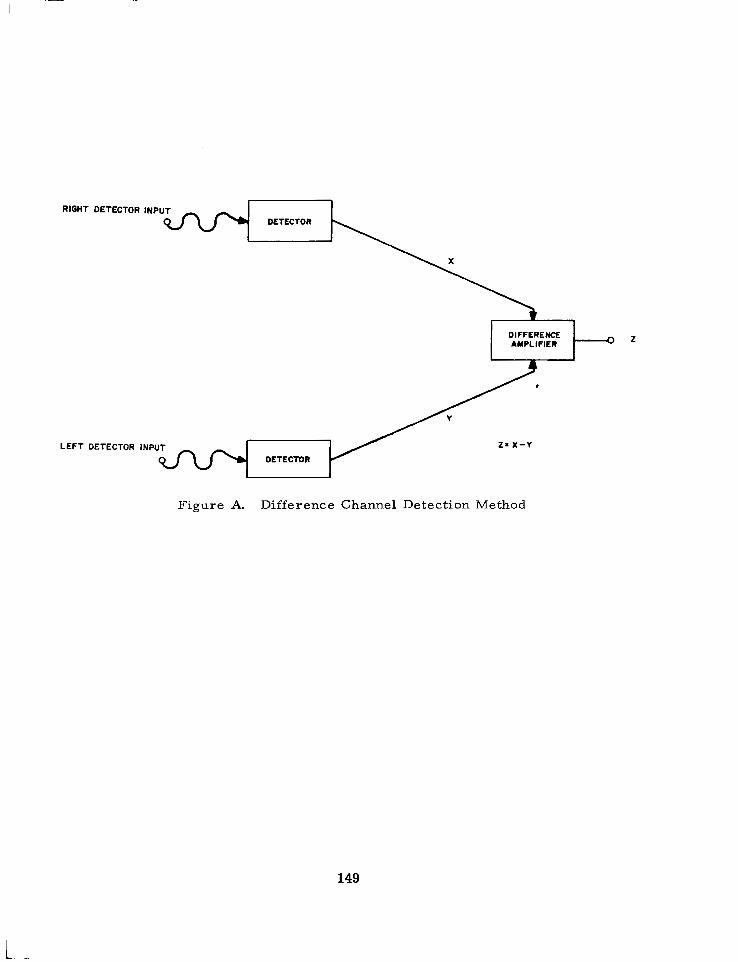
RIGHT DETECTOR INP DETECTOR
DIFFERENCE AMPLIFIER ’ 0
L E F T DETECTOR INP z = x - Y
DETECTOR
Figure A. Difference Channel Detection Method
149
L. .

System Theory Modulation Methods
OPTICAL PCM POLARIZATION MODULATION
where
'S, B = average number of signal photoelectrons released by right detector per bit interval
p N y B ' re leased by right detector per bit interval
pN' B' re leased by left detector per bit interval
= average number of right channel noise photoelectrons
= average number of left channel noise photoelectrons
In t e r m s of the detection statistics the probability of detect ion error is
If the average value of the shot noise is the same in both detectors let
t*N, B 'N, B, R = 'N. B, L E 2
then the probability of detect ion error can be wri t ten in terms of modi- fied bessel functions.
Figure B shows the probability of detect ion error for the PCM/PL system as a function of the signal and noise photoelectron counts.
150
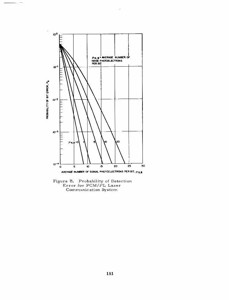
lo-'
10-2
10-5
10-4 I5 20
I
L
25 30
AVERSE NUMBER OF S I W L PHOTOELECTRONS PER BIT. /AS,B
Figure B. Probability of Detection E r r o r for PCM/PL Laser
Communication System
151

System Theory Modulation Methods
OPTICAL PCM FREQUENCY MODULATION
By assuming Gaussian statistics, an expression for probability of e r r o r is derived and plotted for optical frequency modulation.
In the optical PCM frequency modulation system information is conveyed by t ransmission of the carrier at one of two different frequencies to represent "one" and "zero" bits. Demodulation could conceivably be performed by placing two optical filters, centered at the two possible carrier frequencies, before a pa i r of photodetectors. The detection model would then be the same as that for polarization modulation. How- ever, optical f i l ters at present are extremely wide band and do not exhi- bit sharp frequency cutoff properties. Therefore, spectral isolation of the transmitted frequencies is not simple. Frequency demodulation may be performed by heterodyning the laser carrier to an IF frequency where a standard radio frequency FM receiver can provide frequency detection.
Unfortunately, little is presently known of the detection statistics of a heterodyne receiver. It is possible, however, to determine an expres- sion for the probability of e r r o r of a heterodyne PCMIFM system by assuming that the IF output noise is Gaussian. Then, from the theory of radio frequency detection, the probability of e r ror a t the FM rece iver output is
P = - exp 1 e 2
where [ ~ / N ] I F is the signal-to-noise ratio at the IF output of the hetero- dyne receiver. The Figure gives the probability of de tec t ion e r ror as a function of the signal photoelectron counts.
'Prat t , W. K., "Binary Detection in an Optical Polarization Modulation Communication Channel, IEEE Transactions on Communication Technology, October 1966.
152

I-
IO" I
t Probability of Detection Error for
PCM/FM Laser Communication System
153
L

System Theory Modulation Methods
OPTICAL PPM INTENSITY MODULATION
Probability of b i t e r ror for a PPM intensity modulated optical carrier is derived and plotted as a function of signal and background photoelectrons.
In the optical PPM system, signal photons are transmitted in one of L t ime slots. Let
PSN = probability that the signal plus noise photoelectron count P
equals or exceeds the decision threshold NT during a sample period.
PN = probability that the noise photoelectron count equals or P
exceeds the decision threshold N during a sample period. T
Then, based upon Poisson detection statistics, the signal plus noise and noise detection probabilities are
i
i=N P i ! t
where
= average number of signal photoelectrons emitted by " 9 photodetector per sample period
pN, = average number of noise photoelectrons emitted by photodetector per sample period
The optimum threshold Nt 1s the greatest integer value of the likelihood ratio threshold ktP where
P .
154

w h e r e
pi = a p r i o r i p r o b a b i l i t y of t r a n s m i t t i n g a s igna l i n . t he ith s lo t . -
The probabi l i ty of a s a m p l e e r r o r is then
probabi l i ty tha t no ise equals o r exceeds th reshold before s igna l s lo t 3
p robab i l i t y t ha t no i se equa l s o r exceeds t h re sho ld a f t e r s igna l s lo t , g iven s igna l p lus no i se does no t equa l o r exceed t h re sho ld 1 probabi l i ty tha t ne i ther no ise p robabi l i ty of no r s igna l p lus no i se equa l s i n c o r r e c t r a n d o m o r e x c e e d s t h r e s h o l d choice 1
Then,
L i - 1 L
P I e = 1 pi [ I - (1 - PNp) 3 + 1 pi (1 - pNp)i- l (1 - PspN)
i= 1 i= 1
L- 1 L
[ l - (1 - P.')L-i] t ( 1 - P C ) (1 - PspN) 1 P i ( l - p i )
i= 1
For a uniform source distribution, p = 1/L, the probability of e r ro r is i
P e k S N -
The Figure illustrates the probability of detection error as a function of the signal and noise photoelectron counts per sample period.
155
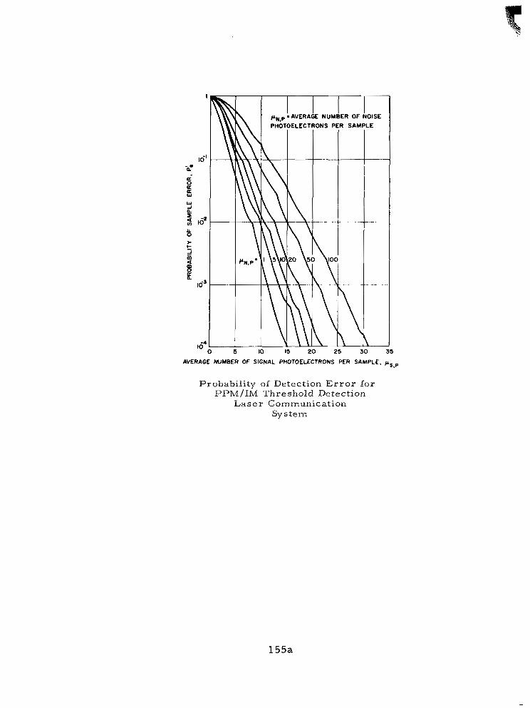
,A4 L
"i== NUMBER OF NOISE
INS P
""
-. - ..
t L
.E
'" 0 IO I5 20 25 30 35
AVERAGE NUMBER OF SIGNAL PHOTOELECTRONS PER SAMPLE. psSp
Probability of Detection Error for P P M / I M Threshold Detection
Laser Communication System
155a

System Theory Modulation Methods
4
RADIO AMPLITUDE, FREQUENCY, AND PULSE CODE MODULATION
Signal to noise ratio relationships are given for amplitude and frequency modulation and probability of error relationships are given for pulse code modulation.
Figure A illustrates the components to be considered for either an analog or digital radio communication system.
Radio Amplitude Modulation
In the radio amplitude modulation (AM) system the amplitude of the car- rier is directly proportional to the amplitude of an information signal.
Radio A M transmission is normally done in one of three ways, conven- tional AM (carr ier present) , double sideband AM ( n o carr ier present) , and single sideband AM ( n o carr ier present) . An important relationship in these three transmission variations is the relationship of the radio frequency or intermediate frequency signal to noise ratio [S /N] IF to the signal-to-noise ratio at the output of a peak detector, [S /N]D, measured in the information bandwidth, B. These relationships are given below. It should be noted that the r-f o r i - f bandwidth required for single side- band AM i s one half that of double sideband AM and conventional AM,
F o r conventional AM
2 [$ID = 1 ma 2][g] For [;IIF > 10 l t m I F a
where m is the modulation index ( 0 < ma < 1 ).
For double sideband AM
a
[:ID = [;I I F
For single sideband AM
Radio Frequency Modulation
In the radio frequency modulation system the frequency of the c a r r i e r is set proportional to the amplitude of an information signal. The in- stantaneous phase + ( t ) of the carrier is
C
156

, . . ._. . . . I ._...-... ............ -...I.... ,...,., "".".".. "I-.""."-.. I..,. .I,. . I." .. .I ..I.. ... .. , . I. ".. ..I. "". .. ,, ., ".
t
where x(t) represents the information signal and mf is the frequency modulation index (mf = peak carrier frequency deviation/modulating frequency).
The relationship between the r-f o r i - f signal to noise ratio, [S/N]IF, measured in a bandwidth BIF and the detected signal-to-noise ratio measured in a bandwidth, B, for a sine wave modulation of frequency fm, is given by:
Radio PCM Amplitude Modulation
In the radio PCM/AM system, a s igna l car r ie r is transmitted for a "one" bit and no signal carrier is transmitted for a "zero" bit. The probabi- lity of detection error for detection in the presence of white Gaussian noise is. 1
. "" ~.
Noncoherent Detection ~. .
Coherent Detection
where K is defined by
- = dn Io 2E
NO
'Lawton, J. G. , "Comparison of Binary Data Transmission Systems, Proceedings Second National Convention on Military Electronics,, 1958.
157

System Theory Modulation Methods
RADIO AMPLITUDE, FREQUENCY, AND PULSE CODE MODULATION
and where
E = signal energy per bit
N = noise power spectral density 0
Figure B shows the probability of detect ion error as a function of the ratio E/No.
Radio PCM Freauencv Modulation
In the radio PCM frequency modulation system information is conveyed by t ransmission of t he ca r r i e r a t one of two frequencies to represent "one" and "zero" bits. The probability of detection error for detection is the presence of white Gaussian noise is :::.
Noncoherent Detection
Pe = 2 exp 1
Coherent Detection
Figure B shows the probability of detect ion error as a function of the ratio E/No.
Radio PCM Phase Modulation
In the rad io PCM/PM sys tem, the car r ie r is t ransmit ted at one of two phase angles 180 degrees apar t to represent "one" and "zero" bits. The probability of detection error for detection in the presence of white Gaussian noise is,
Coherent Detection
Differentially Coherent Detection "
pe = 7 exp 1- e} 1
The Figure shows the probability of detect ion error as a function of the rat io E/N,.
158

I I
. MODULATOR
MOWUTOR D I l v E R
I
I I L """"" "-1
RANSMITTER
0 . FUNDAMENTAL ANALOG I-F COMMUNICATION SYSTEM
I fc + ' m n I +SIDEIANM I I - F
I AhVLIFIEI
ANALOG TO DIGITAL CONVERTER INCLUDES SAMPLER AND CODER, i _ e _
SIGNAL SOURCE
L""""""l HETERODYNE RECEIVER
DIGITAL TO ANALOG CONVERTER
1
I
SIGNAL, FRONT END 'IF UP THROUGH FILTER "c DECODER
SIMILAR TO ABOVE IF N.4PLIFIER.
RECEIVER
SIMILAR TO THE ABOVE
I MATCHED
I DETECTOR
I I I
1 I LOW-PAIS
f i T b . FUNDAMENTAL DIGITAL SYSTEM FILTER.
I L"""
F i g u r e A. F u n d a m e n t a l A n a l o g ( R F ) a n d D i g i t a l ( R F a n d / o r O p t i c a l ) C o m m u n i c a t i o n S y s t e m s , B l o c k D i a g r a m
F i g u r e B. P r o b a b i l l t y of D e t e c t i o n E r r o r f o r P C M R a d i o
C o m m u n i c a t i o n S y s t e m s
.- -14 -IO -# -L 0 2 6 10
a 14 SCLCTRAL DCWSITY RATIO €/No 111 DE
SIG11AL EUCROY TO U018L POWER
159
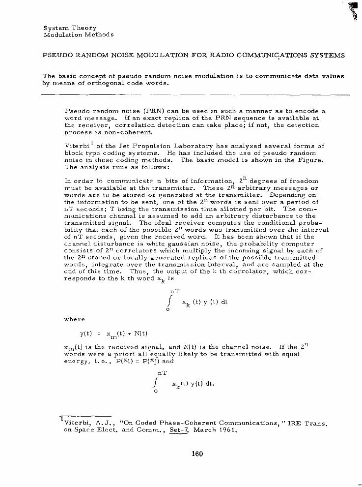
System Theory Modulation Methods
PSEUDO RANDOM NOISE MODULATION FOR RADIO COMM.UNICbATIONS SYSTEMS
The basic concept of pseudo random noise modulation is to communicate data values by means of orthogonal code words.
Pseudo random noise (PRN) can be used in such a manner as to encode a word message. If an exact replica of the P R N sequence is available at the receiver, correlation detection can take place; i f not, the detection process is non-coherent.
Viterbi' of the Jet Propulsion Laboratory has analyzed several forms of block type coding systems. He has included the use of pseudo random noise in these coding methods. The basic model is shown in the Figure. The analysis runs as follows:
In order to communicate n bits of information, Zn degrees of freedom must be available at the transmitter. These 2n arbi t rary messages or words are to be stored or generated at the transmitter. Depending on the information to be sent, one of the 2n words is sent over a period of nT seconds; T being the transmission time allotted per bit. The com- munications channel is assumed to add an arbitrary disturbance to the transmitted signal. The ideal receiver computes the conditional proba- bility that each of the possible 2n words was transmitted over the interval of nT seconds, given the received word. It has been shown that i f the channel disturbance is white gaussian noise, the probability computer consists of 2n correlators which multiply the incoming signal by each of the Zn stored or locally generated replicas of the possible transmitted words, integrate over the transmission interval, and are sampled at the end of this time. Thus, the output of the k th correlator, which cor- responds to the k th word xk is
where
'Viterbi, A . J., "On Coded Phase-Coherent Communications, ' I IRE Trans. on Space Elect. and Comm., Set-7, March 1961.
160

It follows intuitively that in order to achieve low error probabilities, the waveforms should be as unlike as possible, such that in a noisy channel there will be the least possible chance to make the wrong selection of the word transmitted. More precisely, the cross-correlation coefficients among all pairs of words,
nT r
P = 1 xi (t )x. (t )dt n J - ~ _ _ _ ~ . . [TTp x:(L)dt + x. (t)dt
nT 2
O J I”’ should be as low as possible. Low cross correlation coefficients are obtained by various coding combinations.
L$gh- MESSAGES
\ MESSAGE SELECTOR
CORRELATORS MESSAGES STORED
1
DECISION DEVICE
7- OUTPUT
I
L ”””””- 1 I
MESSAGE STORED
ONE OF THE 2“ CORRELATORS
The Basic Model
161

J

SYSTEM THEORY
Communication Coding
Page Data Compression . . . . . . . . . . . . . . . . . . . . . . . . . . . . . . . . . . . . . . . . . . . . . . . . . . . 164
Synchronization . . . . . . . . . . . . . . . . . . . . . . . . . . . . . . . . . . . . . . . . . . . . . . . . . . . . 166
163

System Theory Communication Coding
DATA COMPRESSION
Data compression can be applied to engineering data, scientific data, or pictorial data. The reduction in equivalent bit rate is as high as a factor of 10.
"" - ~~
A generalized block diagram of the coding elements of a communication system is shown in the Figure. The source coder at the t ransmit ter is the equipment that converts the source data - e. g. , T V , voice, scientific information - into a sequence of code bits of minimum possible length. The receiver source decoder performs the inverse operation of reproduc- ing the source data from the code bits. The operation of source coding and decoding is denoted as data conditioning and reconstruction.
The channel coding equipment a t the transmitter puts the source message sequence in a form that will minimize the effects of channel noise. At the receiver the channel decoding equipment reconstructs the source mes- sage sequence. The channel coding and decoding operations are per- formed by the format coding and decoding equipment. In addition, the format coding operation consists of message arrangement and identifica- t ion for transmission.
Data Compression
Data conditioning offers the possibility of an increase in the information ra te of a communication system after optimum coding and modulation techniques have been applied to the system, and when the physical limits of communications equipment have been reached. The information rate increase is realized by transforming the source data, by an elimination of redundancy, into a form in which fewer symbols are required to describe the data. The theoretical possibilities of this type of data com- pression for voice and picture communication are enormous. Data com- pression for scientific and engineering data is a function of the type of data but, in general, scientific data is capable of a large amount of r e - duction. The Table presents estimates of source bit rate reduction pos- sible with vario.us techniques of compression schemes.
It would be desirable to employ a single, simple data compression device for all c lasses of data in a generalized communication system. However, such a device has not been developed or even approached to date. The most promising path to the realization of a general ized data compressor in the near future seems to be the development of separate compression schemes for the three main c lasses of data - pictorial, speech, scientific, or engineering. In such a system, the physical characterist ics of each c l a s s of data can be employed to realize practical data compression most efficiently.
164

r
SOURCE CODERS
Source Bit Rate Reduction
DESTINATION DECODERS
SOURCES
CL Q, ul
PICTORIAL
CONDITIONING
CHANNEL CODER
CHANNEL DECODER
PICTORIAL
RECONSTRUCTION
SCIENTIFIC AND ENGINEERING
CONDITIONING
a. Transmit t ing System
Type of Data
Scientific
Engineering
Pictorial information (real-time TV)
Voice
Bandwidth
0 to 1 KHZ
0 to 1 KHE
4 MHZ
4 KHZ
Equivalent PCM
u p t o 18 kilobits/ second
u p to 18 kilobits/ second
48 megabits/ second
40 kilobits/ second
Communication Coding
Source Bit Rate Reduction ~~
Delta Coding
Stop Scan Edge
Detection
24 megabits/ second second 12 megabits/
: 20 kilobits I second
SCIENTIFIC AND ENGINEERING
RECONSTRUCTON U
Multiple
Encoding Coding
kilobitel Up to 6
second
Up to 6 kilobits1 second
12 megabits/ second
~
Vocoding
kilobits/ 3 to 6
second
TO DESTlNATIoll

System Theory Communication Coding
SYNCHRONIZATION
Time synchronization is required for digital transmission, a variety of synchronizing methods are received.
Time division modulation systems, such as PCM and PPM, require synchronization between the transmitting and receiving equipment to en- sure accurate decoding. The degree to which synchronization is estab- lished directly affects the signal-to-noise performance of a communica- tions system.
Accurate timing references can be generated at the receiving terminal of a PPM communication system by using synchronization information con- tained in the transmitted waveform without using additional transmitter power for this purpose. Synchronization can best be made where each successive waveform is guaranteed to possess a unique characterist ic or where each succeeding waveform is guaranteed to be in some way dif- ferent from its predecessor. For example, a PPM system may convey frame synchronization by making one of i ts bursts of information wider than any other in the sequence.
In PCM modulation systems, a receiving station must lock in frequency and phase on the transmitted digital rates to fulfill its requirement to gain synchronization. This lock must be achieved and maintained even when the transmission medium is noisy for the data to be interpreted correctly. The synchronizer must have the ability to detect transmitted sync codes even when they are corrupted with erroneous bits, to verify that the detected codes are transmitted periodically, to compute the de- tected code frequency of occurrence, and to measure the mean error rate to ascertain whether or not the detected code is compatible with the expected code. Usually several levels of synchronization exist concur- rently in a PCM telemeter format - bit, word, frame, and subframe synchronization.
The PCM synchronizer must operate in three different modes: ( 1 ) the search mode during which the synchronizer looks throughout the trans- mitted PCM data for the synchronization pattern; ( 2 ) the check mode during which the synchronizer verifies that the pattern found in search does occur periodically, which will increase the probability for that pattern to be transmitted synchronization code; and ( 3 ) the lock mode during which the synchronizer will put the emphasis on its fly-wheel characteristics to maintain lock as long as the mean error ra te is compatible.
Word synchronization has been accomplished by the separation of words in time by a pulse of a different amplitude, or by a special code consist- ing of a few bits. Because of its bandwidth requirements, word synchron- ization has fallen into disuse. Frame synchronization is usually accom- plished by transmitting a special code every time the basic commutator recycles. This code must be detected by the frame synchronizer, which in turn resets the decommutator word-per-frame counter. Whenever the telemeter format involves a solid word synchronization, it is possible to forbid the generation of any given code sequence, and therefore the frame sync code pattern is unique, but only i f a noise-free transmission link is assumed. In the absence of word sync patterns, uniqueness is impossible
166
I
to preserve s ince adjacent port ions of sequential words may create a spurious code pattern. A known solution for the problem of quasi-static data, which may construe data bits into a sync code pattern, is the alter- native transmission of sync code patterns and their binary complements. This method will completely eliminate the possibility of not acquiring a sync because of the presence of quasi-static data.
Subframe synchronization utilizes two different methods. One - the r e - cycling method - consis ts of transmitting a code pattern during the basic frame where the subcommutator recycles. This code can be transmitted where the subcommutated primary channel would have a predetermined position within the primary frame independent of the location of the sub- commutated channel. The other method - countdown - consis ts of t rans- mitting the number corresponding to the segment position of the subcom- mutator every frame. This method requires more bandwidth than the recycling method. The countdown method permits on the average a fas te r subcommutator sync acquisition but is extremely vulnerable to noise and should be used only where the error ra te is expected to be low.
A synchronization process that may be used in a te lemetry system is a unique combination of the basic properties of phase-lock groups and quasi-random binary sequences, commonly called pseudo-noise ( P N ) sequences. A P N sequence, which is odd in length, when phase com- pared with a duplicate of itself does not look like this duplicate until both sequences are in perfect alignment. Therefore, this process is capable of producing a unique sync pulse rate. The autocorrelation function i f a P N sequence is obtained by comparison of adjacent bits in the duplicate sequences. The autocorrelation function - (number of similar bits - number of dissimilar bits)/ total number of bits in sequence -will have its numerator equal to 1 whatever the sequences are not in alignment and will equal 0 whenever the sequences are aligned.
167


SYSTEM THEORY
Telemetry Communications
Page FM and FM/FM Link Equations . . . . . . . . . . . . . . . . . . . . . . . . . . . . . . . . . . . . . . . . . . . 170
Degradation Caused by Nonideal Postdetection Filtering . . . . . . . . . . . . . . . . . . . . . . . . . . . . . 174
169

System Theory Telemetry Communications
FM AND FM/FM LINK EQUATIONS'
FM improvement formula are given for FM links and FM l inks using FM subcarriers (FM/FM).
Introduction
The elements of a typical FM or FM/FM t ransmission l ink are shown in the Figure. An FM link would begin at the modulator input, and termin- ate at the carrier demodulator output (after postdetection filtering). The modulating data signals considered will be assumed sinusoids; however, this is not a limitation, since the postdetection SNR derived can be con- sidered to apply to aperiodic signals during their time of occurrence.
The FM/FM link in its most general sense will employ i subcar r ie rs , of different center frequencies and deviations, each frequency modulating the carr ier .
TABULATION O F SNR IMPROVEMENT FORMULAE
The glossary of t e r m s is given at the conclusion of this topic. Sinusoidal signal modulation is presumed.
Single FM (same as second detection in FM/FM link)
Carson 's rule s ta tes that the if bandwidth, bif = 2 f m ( m t l ) = 2 f m
$or ideal link elements, 6, the degradation factor, is set at z 1. 0.
Otherwise, a value of 6 can be selected from the appropriate Figures given in the following topic.
A more general form of Equation ( l ) , which can be used below threshold (defined as the departure from linearity on the SNR transfer character is- tic) is given below2
'Rechter, Robert J . , "Summary and Discussion of Signal-to-Noise Ratio Improvement Formulae for FM and FM/FM Links, " International Telemetry Conference Proceedings, L, October 1967, p. 172.
No. ERL-8-0009-623, Electronics Research Laboratory. 2Duncan, John, "FM Demodulator Threshold Reduction, ' I Final Report,
170

RE SUBCARRIER OSCILLATOR,
SCO, GAIN AND "--, FILTER NETWORK,
SUBCARRIER
NETWORK "r, SCO NO. 1 AND FILTER OSCILLATOR
POST SCO GAIN I
f s I fsc I 1 HI . e . MODULATOR
PRE-EMPHASIS e . .
DATA SIGNALS : 0 . SUMMING
AMPLIFIER e . NETWORK
'INK TRANSMITTER +
0 0 . K l
PRE SCO GAIN AND FILTER NETWORK
SUBCARRIER POST SCO GAIN OSCILLATOR
fsi Hi fsc i
AND FILTER "--* NETWORK - sco NO. i
TRANSMITTING STATION
RECEIVING STATION """"""""""
r ,
------i___h. POSTDETECTION FILTERING
F M
I
CARRIER
FILTER NO. c - FILTER NO. 1 NO. 1
SUBCARRIER SUBCARRIER SUBCARRIER -J PRE-DETECTION
FILTER
CARRIER RECEIVER DEMODULATOR PREDETECTION DISCRIMINATOR POSTDETECTION
K2 Bl f Bsc 1 K3 fsl
SUBCARRIER SUBCARRIER PREDETECTION DISCRIMINATOR POSTDETECTION
SUBCARRIER
FILTER NO. i NO. I NO. 1 "*
Bsci K3 t
Typical FM or FM/FM Transmission Link

System Theory Telemetry Communications
FM AND FM/FM LINK EQUATIONS
For SNRif >> 1, i. e., the above-threshold case, Equation 2 simplif ies to Equation 1.
Subcarrier Predetection SNR Relat ive to Carr ier SNR, i n FM/FM Link __ ~ ~.
This is the general form of the equation; for subcarrier peak deviations small in comparison with subcarrier center frequency (i. e . , the IRIG channels) Equation 3 can be simplified to
Subcarrier Postdetection SNR, Relat ive to Carr ier Predetect ion SNR, in a FM/FM LinkTFverall SNR)
The general relationship, for sinusoidal modulation, using the approxi- mation of Equation 4.
0. 375 BifBsci(Afci) Afsci 2
oi ( fsci) (fsi) 2 3
Bif =
Bsci =
f C - -
f . =
f lbe i =
fubei =
f . =
sc1
s1
f m
Aft =
- -
Carrier predetection equivalent noise bandwidth, Hz
Predetection equivalent noise bandwidth of i th subcarr ier , Hz
Carrier center f requency, Hz = / 2 ~ r
Center frequency of i th subcarr ier , Hz
Lower bandedge frequency of i th subcarr ier , Hz
Upper band edge frequency of i th subcarr ier , Hz
Subcarrier postdetection equivalent noise bandwidth, Hz
Carrier-modulating data baseband, Hz
Peak carr ier deviat ion
172

, .,.",._ "..,._..."._. ...
Afci
Afsci Afci/fscl = Modulation index of ith subcarrier on the carrier, radians
Afsci/fsi = Deviation ratio or ith data signal-subcarrier, radians
(S/N)sci = Signal-to-noise (SNR) ratio in ith subcarrier predetection
= Peak carrier deviation due to ith subcarrier, Hz
= Peak deviation of ith subcarrier center frequency, Hz
bandwidth, dB
(S/N)if = Carrier predetection SNR
(S/N)oi = Postdetection SNR of ith subcarrier channel
(S/N)o = Post detection SNR.
173

System Theory Telemetry Communications
DEGRADATION CAUSED BY NONIDEAL POSTDETECTION FILTERING
The degradation caused by postdetection filtering is given for Butterworth, Bessel, .and Chebyshev filter functions.
Only in an ideal link is the postdetection degradation factor, 6 , unity (see prior topic). Assuming that the degradation of SNR from theoretical rests mainly in the nonideal nature of the FM demodulator postdetection (output) filter, allows the use of Figures A through C(4) to give 6 in logar- ithmic notation for the Butterworth, Bessel, and Chebyshev filter func- tions. These figures clearly show the very significant degradation due to low order postdetection filtering. For instance, a first order function would result in infinite output noise power, for the mathematically ideal case, since the asymptotic slopes of the noise and filter functions cancel. Even a second order Butterworth results in a 6 2 5. 2 db.
The factor 6 is computed as follows
defining
N as the spectral density (usually presumed quadratic)
G. as the postdetection filter amplitude transfer
0
3 The total noise power transmitted by a physically realizeable output filter can be computed as follows:
The noise power transmitted by a zonal filter, i. e. , a filter which has the amplitude transfer characteristic
G. = 1 over the baseband, f : J S
E 0 elsewhere
is given by
and the degradation factor, 6 , is computed as
6 = 10 Log [%] db

Assumptions and Deviations from Ideal Modeling
The degradation 6, from ideal SNR improvement previously defined, presumed quadratic postdetection noise spectral density. In actuality, nonzonal predetection filtering will tend to make the postdetection noise spectrum less than quadratic, thus reducing the magnetude of 6, as can be observed in Figure D, i f Bif/2 >>fsi, is the baseband. In any case, a precise evaluation of 6 would require proper shaping of the output noise spectrum, to account for nonzonal predetection filtering.
3 4
1
DEGRADATION IN db OF NTH ORDER
ON QUADRATIC NOISE SPECTRUM, BUlTERWORTH FILTER.OPERATING
WITH RESPECTTO BRICKWALL FILTER
-
I 6 6 7 8 9 10
NUMBER OF POLES, ORDER
Figure A
DEGRADATION IN db OF NTH ORDER
QUADRATIC NOISE SPECTRUM, WITH BESSEL FILTER, OPERATING ON
RESPECT TO BRICKWALL FILTER
2 3 4 5 6 7 8 9 10
NUMBER OF POLES, ORDER
Figure B
175

a - i I 1 I DEGRADATION IN db OF NTH ORDER CHEBYSHEV FILTER, 1.0 db RIPPLE
6 FACTOR, OPERATING ON QUADRATIC NOISE SPECTRUM, WITH RESPECT TO BRICKWALL FILTER
4 I I I
2
0 17 Y-rl'\-l//-l-\l
-2 2 3 4 5 6 7 8 "I 9 10
NUMBER OF POLES, ORDER
Figure C (a)
8 ." - - .. ~
DEGRADATION IN db OF NTH ORDER CHEBYSHEV FILTER.2.0 db RIPPLE
NOISE SPECTRUM, WITH RESPECT TO 6 FACTOR, OPERATING ON QUADRATIC -
0) -I w
0 m BRICKWALL FILTER - B 4
0 i k a U 9 2 "_ 1 : -
:: 0
0
-2
2 3 4 5 6 7 8 9 10
NUMBER OF POLES, ORDER
Figure C (c)
176

1 1 1 - -
l o I I I I I I I I
8
2
0 2 3 4 5 6 7 8 9 10
NUMBER OF POLES, ORDER
Figure C (b)
DEGRADATION IN db OF NTH ORDER CHEBYSHEV FILTER, 3.0 db RIPPLE FACTOR, OPERATING ON OUADRATIC - NOISE SPECTRUM, WITH RESPECT TO BRICKWALL FILTER
0 i
a l-
0 2 3 4 5 6 7 8 9
NUMBER OF POLES, ORDER
Figure C (d)
177
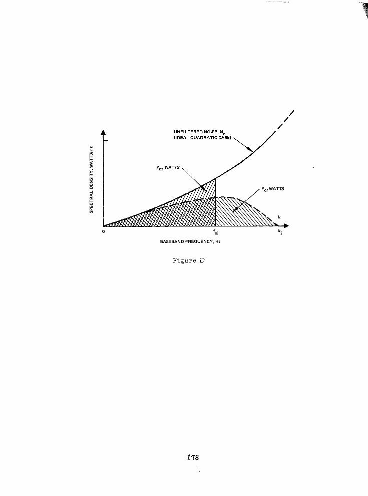
. "
/ /
/ UNFILTERED NOISE, No (IDEAL QUADRATIC CASE)
2 5 9 < t
a v) z YI
J
2 I- o n YI Lo
0 si k.
BASEBAND FREQUENCY, Hz
Figure D

APPENDIX A
COMMUNICATION SYSTEMS OPTIMIZATION METHODOLOGY

APPENDIX A
COMMUNICATION SYSTEMS OPTIMIZATION METHODOLOGY
A. 1 INTRODUCTION
The complexity of evaluating the relative roles of sys tems for
future spacecraf t communicat ion and t racking appl icat ions, consider-
ing the broad spectrum of potential manned and unmanned space mis-
sions, demands a unified methodical approach. As shown in Figure A-1,
the t ask is one of examining the study data compiled by communication
components analysis, and communication systems analysis studies; and
then determining the opt imum parameters for communicat ion systems.
In brief, the communication components analysis task provides data on
the system parameters with re la t ionship to the fabr icat ion cost , weight ,
s ize , e tc . , of the component implementation. The communication sys-
tems analysis provides the re la t ionships between the communicat ion
parameters , noise effects , and system constraints . While the general
goals of the systems optimization task can be stated rather simply, its
implementat ion wil l require a significant amount of effort due to the
large number of parameters that must be considered.
This communication systems optimization methodology section is
divided into sub-sections which treat the general optimization procedure
for communication systems, followed by examples of the optimization
procedure. The section concludes with a design methodology which
summar izes the resu l t s of the optimization methodology for optical and
radio systems, and presents short cut methods of evaluating systems.
A.2 COMMUNICATION COMPONENTS ANALYSIS
The communication components analysis task is i l lustrated by the
flow chart of F igure A-2. For each component the weight, fabrication
cost , power requirement , and power diss ipat ion are der ived as a func-
t ion of the sys tem parameters . A total component cost is developed as
the sum of the fabr icat ion cost and cost of placing the component weight
aboard a spacecraf t , i f applicable.
A- 1

COMMUNICATION COMPONENTS
ANALYSIS
SYSTEMS EVALUATION
COMMUNICATION
ANALYSIS SYSTEMS
Figure A-1. Systems optimization f low chart .
TRANSMITTER ANTENNA BURDENS I"@ RECEIVER ANTENNA BURDENS I-@
TRANSMITTER ACQUISITION AND TRACK SYSTEM BURDENS
RECEIVER ACQUISITION AND TRACK SYSTEM BURDENS
TRANSMITTER BURDENS
MODULATION EQUIPMENT BURDENS
DEMODULATION EQUIPMENT BURDENS I-@ TRANSMITTER POWER SUPPLY BURDENS
RECEIVER POWER SUPPLY BURDENS
TRANSMITTER AND RECEIVER PARAMETERS
Figure A-2. Communication components analysis flow chart.
A- 2

0 C1. Transmit ter Antenna Burdens
The weight and fabrication cost of a t r ansmi t t e r an t enna a r e
propor t iona l to the t ransmi t te r aper ture d iameter . The t ransmi t te r
antenna weight is
n W = K (aT) + WKT T
dT dT
and the fabrication cost is
where
dT = t r ansmi t t e r ape r tu re d i ame te r
KdT t ransmi t te r aper ture d iameter
K = constant re la t ing t ransmit ter antenna fabr icat ion cost
= constant re la t ing t ransmit ter antenna weight to
'T t o t r ansmi t t e r ape r tu re d i ame te r
WKT = transmitter antenna weight independent of t ransmi t te r
CKT = transmitter antenna fabrication cost independent of
aper ture d iameter
t ransmi t te r aper ture d iameter
nT = constant
mT = constant
The total cost associated with the transmitter antenna is the fabrication
cost and the cost of placing the weight W aboard a spacecraft . Thus, dT
where
K = cost per unit weight for spaceborne equipment S
A- 3

0 C2 Receiver Antenna Burdens
The weight and fabrication cost of a rece iver an tenna a re
proport ional to the receiver aper ture diameter . The receiver antenna
weight is
nR W = K (dR) t WKR dR dR
and the fabrication cost is
where
dR = rece iver aper ture d iameter
dR aper ture d iameter
'R rece iver aper ture d iameter
K = constant re la t ing receiver antenna weight to receiver
K = constant re la t ing receiver antenna fabr icat ion cost to
WKR = receiver antenna weight independent of rece iver
CKR = receiver antenna fabrication cost independent of
aper ture diameter
rece iver aper ture d iameter
nR = constant
mR = constant
The total cost associated with the receiver antenna is the fabr icat ion
cost and the cost of placing the weight W aboard a spacecraf t . For
opt ica l sys tems there is an additional fabrication cost due to fabrication
of a high quali ty short focal length aperture when the receiver f ield of
view is much larger than the diffraction limit, but this additional cost
is usual ly negl igible with respect to the aper ture diameter dependent
cost . The total receiver antenna cost is then
dR
A-4

@ Transmit ter Acquis i t ion and Track System Burdens
The t ransmit ter must i l luminate the receiver under f ixed
acquisit ion t ime limits and then maintain an angular tracking accuracy.
Acquisition and tracking equipment consists of a gimbal system to s lew
the t ransmit ter antenna to the desired point ing angle , a sensor to detect
the l ine of s ight rotat ional error between the t ransmit ter and receiver
by monitoring a communication or beacon signal emitted from the
receiving site, and a s table platform reference for the sensor . The
acquisit ion and tracking sensor signal may be obtained from 1) a secon-
dary antenna, 2 ) the t ransmit ter antenna act ing as a receiving antenna
on a shared bas i s , o r 3 ) the antenna of a communications receiver i f
avai lable a t the t ransmit ter . A beacon a t the t ransmit ter used by the
rece iver for its acquisition and tracking function will not affect the
system parameters opt imizat ion s ince the beacon burdens are indepen-
dent of the sys tem parameters . Beacon burdens a re cons idered as
pa r t of the f ixed burdens associated with the spacecraf t t ransmit ter
acquisit ion and track system.
The weight and fabrication cost of the acquisition equipment is
relatively independent of the transmitter beamwidth.
The weight of the t ransmit ter acquis i t ion and t rack system is
relatively insensit ive to the tracking accuracy and depends primarily
upon the weight of the transmitter antenna and the weight of the trans-
mit ter sensor , s tabi l izat ion, and acquis i t ion systems. The weight
of the t ransmit ter acquis i t ion and t rack system is
wQT - WBT + KWnT dT - W
o r
A- 5

where
WBT = ' t ransmit ter acquis i t ion and t rack equipment and beacon system weight independent of transmitter beamwidth
= constant relating transmitter tracking equipment weight KWAT to t ransmit ter antenna weight
W = transmitter antenna weight dT
The t racking accuracy requirement may be s ta ted as some f ixed
percentage of the transmitter beamwidth. The fabrication cost of the
tracking equipment is inversely proportional to the tracking accuracy,
and hence, to the inverse of the transmitter beamwidth. Since the
t r ansmi t t e r is diffraction limited, (e - A/dT), the fabrication cost of
the t ransmit ter t racking equipment is proport ional to the t ransmit ter
aper ture d iameter .
T -
The total fabrication cost of the transmitter acquisit ion and
t r ack sys t em is then
o r
where
A =
'AT -
K~~ -
-
-
'T -
qT -
-
-
t ransmission wavelength
t ransmit ter acquis i t ion andtrack equipment and beacon s y s - tem fabr icat ion cost independent of t ransmit ter beamwidth
constant re la t ing t ransmit ter t racking equipment fabr ica- t ion cost to transmitter beamwidth
transmitter beamwidth
constant
The total cost associated with the t ransmit ter acquis i t ion and
t r ack sys t em is
A-6
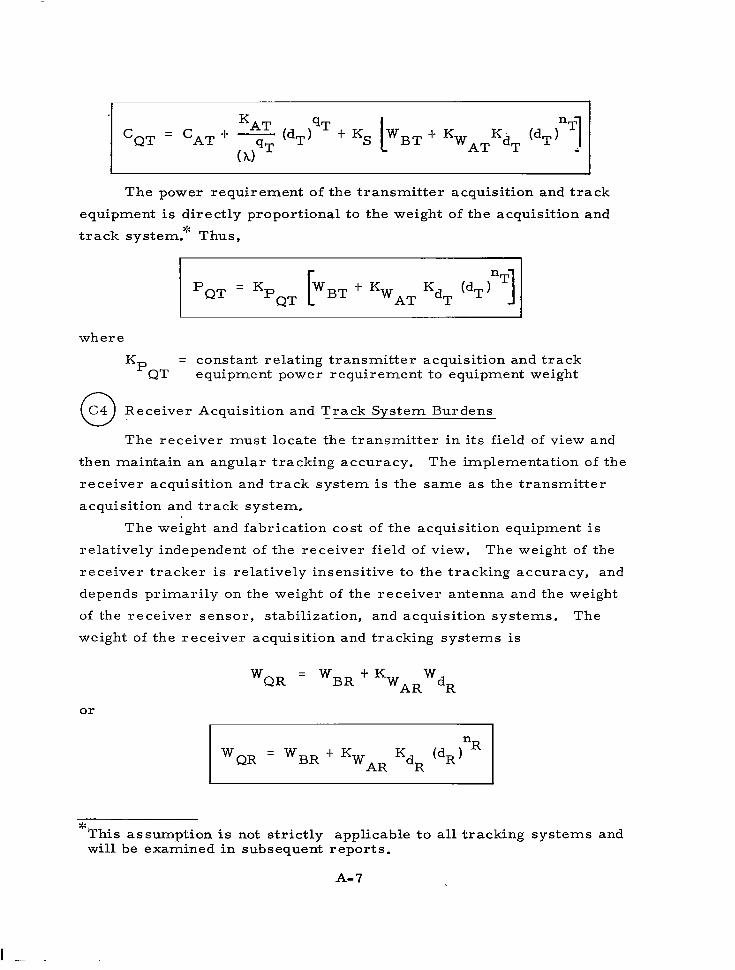
The power requirement of the t ransmit ter acquis i t ion and t rack
equipment is directly proportional to the weight of the acquisit ion and
t r a c k system.". Thus, .L
where = constant re la t ing t ransmit ter acquis i t ion and t rack
KPQT equipment power requirement to equipment weight
0 " C 4 Receiver ~ Acquisition ~~ and Track System Burdens
The rece iver mus t loca te the t ransmi t te r in its field of view and
then maintain an angular tracking accuracy. The implementation of the
receiver acquis i t ion and t rack system is the s ame a s t he t r ansmi t t e r
acquisit ion and track system.
The weight and fabrication cost of the acquisit ion equipment is
relatively independent of the receiver f ield of view. The weight of the
rece iver t racker is relatively insensit ive to the tracking accuracy, and
depends primarily on the weight of the receiver antenna and the weight
of the receiver sensor, stabil ization, and acquisit ion systems. The
weight of the receiver acquis i t ion and t racking systems is
WQR = W B R + K W W~~ d~
o r
*. This assumption is not s t r ic t ly appl icable to all t racking systems and w i l l be examined in subsequent reports .
A- 7

where
= receiver acquis i t ion and t rack equipment and beacon WBR system weight independent of receiver f ie ld of view.
KWAR to receiver antenna weight
W , = receiver antenna weight
= constant relating receiver tracking equipment weight
dR
The t racking accuracy requirement may be stated as some fixed
percentage of the receiver f ield of view. The fabrication cost of the
tracking equipment is inversely proportional to the tracking accuracy,
and hence to the inverse of receiver f ield of view. The total fabrica-
t ion cost of the receiver acquisit ion and track system is then
where
= receiver acquisit ion and track equipment and beacon sys- CAR tem fabr ica t ion cost independent of receiver f ield of view
= constant relating receiver tracking equipment fabrica- t ion cost to receiver f ield of view
qR
eR
= constant
= rece iver f ie ld of view
The total cost associated with the receiver acquisition and. track
s y s t e m is
A- 8

The power requirement of the receiver acquis i t ion and t rack
equipment is directly proportional to ' the wekght of the acquisit ion and
t r a c k system."' Thus, J.
where
= constant re la t ing receiver acquis i t ion and t rack
0 KpQR equipment power requirement to equipment weight
C5 Transmi t t e r Burdens
The weight and fabrication cost of r a d i o t r a n s m i t t e r s a r e p r o -
por t iona l to the t ransmi t te r ou tput power . Laser t ransmi t te rs a re
available only at discrete wavelengths, and each laser is capable of
operation over only a res t r ic ted range of output power by increasing
the laser pumping power; however , at each wavelength within limits
the laser weight and fabr icat ion cost are proport ional to the laser
output power. Thus, the transmitter weight is
and the fabrication cost is
.II -P
This assumpt ion is not strictly applicable t o all t racking systems and wi l l be examined in subsequent reports .
A- 9
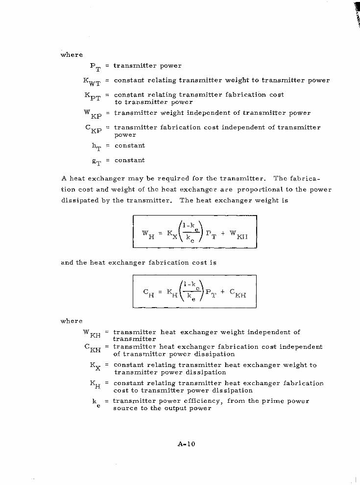
where
PT = t ransmi t te r power
KWT
KpT = constant re la t ing t ransmit ter fabr icat ion cost
WKp = transmitter weight independent of t ransmi t te r power
CKp = t ransmit ter fabr icat ion cost independent of t ransmi t te r
= constant re la t ing t ransmit ter weight to t ransmit ter power
to t ransmi t te r power
power
hT = constant
gT = constant
A heat exchanger may be required for the transmitter. The fabr ica-
tion cost and weight of the heat exchanger are proportional to the power
diss ipated by the t ransmit ter . The heat exchanger weight is
*H - KX ke - (!!) p~ + W~~
and the heat exchanger fabrication cost is
CH - - K H ( F ) PT + CKH
where
WKH = transmitter heat exchanger weight independent of
CKH of transmitter power dissipation
t r a n s m i t t e r = transmitter heat exchanger fabrication cost independent
KX = constant re la t ing t ransmit ter heat exchanger weight to
KH = constant re la t ing t ransmit ter heat exchanger fabr icat ion
t ransmit ter power diss ipat ion
cost to t ransmit ter power diss ipat ion
k = t ransmit ter power eff ic iency, f rom the pr ime power e source to the output power
A-10
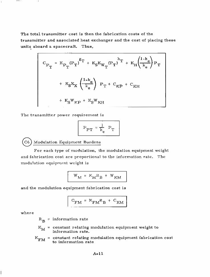
The t o t a l t r ansmi t t e r cos t is then the fabrication costs of the
t ransmit ter and associated heat exchanger and the cost of placing these
uni ts aboard a spacecraf t . Thus,
C = K (PTFT t K K (P,) hT t KH
pT pT wT
' Ks% (2) pT 'Kp ' 'KH
I ' K ~ W ~ ~ ' K ~ W ~ ~ ~ ~~ ~~
~
The t ransmit ter power requirement is
I I
0. C6 Modulation Equipment Burdens
For each type of modulation, the modulation equipment weight
and fabr icat ion cost are proport ional to the information ra te . The
modulation equipment weight is
I wM = K R t W K M I M B
and the modulation equipment fabrication cost is
where
R B = information ra te
KM = constant relating modulation equipment weight to information rate.
KFM = constant relating modulation equipment fabrication cost to information ra te
A-1 1

W~~ = modulation equipment weight independent of information r a t e
CKM = modulation equipment fabrication cost independent of information ra te
The total cost associated with the modulation equipment is the fabr ica-
t ion cost and the cost of placing the equipment aboard a spacecraf t .
Thus, ~~ ~~ ~
- 'M - K ~ ~ R ~ ' 'KM t K S M B K R t KSWKM
The power requirement of the modulation equipment is proportional to
its weight. Thus,
where
K = constant relating modulation equipment power require- pM ment to equipment weight
The modulation equipment burdens include coder burdens,
0 C7 Demodulation Equipment Burdens
The demodulation equipment consists of a ca r r i e r r ece ive r
followed by a subca r r i e r r ece ive r , i f necessary. Also included in the
demodulation equipment is any cooling equipment required to lower the
rece iver t empera ture to reduce dark cur ren t and thermal no ise . For
each type of demodulation system the equipment weight is proportional
to the information rate. The demodulation equipment weight is
and the demodulation equipment fabrication cost is
A - I 2

where
KD = constant relating demodulation equipment weight to
KFD = constant relating demodulation equipment fabrication
WKD = demodulation equipment weight independent of
CKD = demodulation equipment fabrication cost independent of
information ra te
cost to information ra te
information ra te
information ra te
The total cost associated with the demodulat ion equipment is the
fabrication cost and the cost of placing the equipment aboard a space-
craf t . Thus,
'D = K ~ ~ R ~ t 'KD + K ~ K ~ R ~ + K ~ W ~ ~
The power requirement of the demodulation equipment is proportional
to its weight
I P D = K P ~ ~ D ~ B ' KPDWKD 1
where
= constant relating demodulation equipment power require- KpD ment to equipment weight
The demodulation equipment burdens include decoder burdens.
0 C8 Transmitter Power Supply Burdens
The input power requirement of the t ransmit ter specif ies the
power requirement for the transmitter power supply. The power
supply is defined here to include the power source plus voltage or
current conversion equipment. The power supply weight and fabrica-
t ion cost are proport ional to the power requirement . The t ransmit ter
power supply weight is
A-1 3
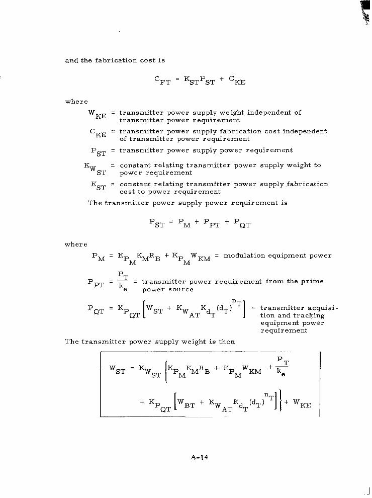
and the fabrication cost is
CFT = K P ST ST -+ 'KE
where
WKE = transmitter power supply weight independent of
CKE = transmitter power supply fabrication cost independent
PST = transmitter power supply power requirement
t ransmi t te r power requi rement
of t ransmi t te r power requi rement
= constant relating transmitter power supply weight to K ~ S T power requirement
KST = constant relating transmitter power supply .fabrication cost to power requirement
The t ransmit ter power supply power requirement is
P~~ = p~ -+ p~~ ' P~~
where
PM = K KMRB + K WKM = modulation equipment power pM pM
pT " - pPT - ke - t ransmi t te r power requi rement f rom the p r ime
power source
p~~ - - KPQT [wST ' KWATKdT (dT)nT] = t ransmit ter acquis i -
tion and tracking equipment power requirement
The transmitter power supply weight is then
A-14

The to ta l cos t assoc ia ted wi th the t ransmi t te r power supply is the
transmitter power supply fabrication cost plus the cost of placing the
equipment weight aboard a spacecraft . Thus,
CST = [KST t K K pT
WST (KPh? KMRB + KpMWKM t--- ke
' KPQT[WBT " KWATKdT (a,)nT] 1 ' KSWKE CKE
0 -
C9 Receiver Power Supply Burdens
The input power requirements of the receiver spec'ify the power
requirement for the receiver power supply. The power supply weight
and fabrication cost are proportional to the
The receiver power supply weight is
WSR = K WSRPSR '
power requirement.
W~~
and the fabrication cost is
'FR - K ~ ~ P ~ ~ + 'KF -
where
W~~ = receiver power supply weight independent of receive,r power requirement
CKF = receiver power supply fabrication cost independent
PSR = receiver power supply power requirement
of receiver power requirement
= constant relating receiver power supply weight to power K ~ S R requirement
KSR = constant relating receiver power supply fabrication cost to power requirement
The receiver power supply power requirement is
PSR = PD + p~~
A-15

where
pD - KpDKDRB " -
pD WKD = demodulation equipment power
requi rement
pQR - - KPQR [WBR " KWARKdR ( d R T R ] = receiver acquis i t ion
and tracking equip- ment power requi rement
The receiver power supply weight is then I
The total cost associated with the receiver power supply is the rece iver
power supply fabrication cost plus the cost of placing the equipment
aboard a spacecraf t . Thus,
I
0 C10 Transmi t te r and Rece iver Parameters
The t ransmi t te r and r ece ive r of an opt ical communicat ion system
are character ized by the fol lowing parameters :
q = quantum efficiency
Id = dark cur ren t
G = photo detector gain
R L = rece iver load res i s tance
Po = local oscil lator power
A- 16.
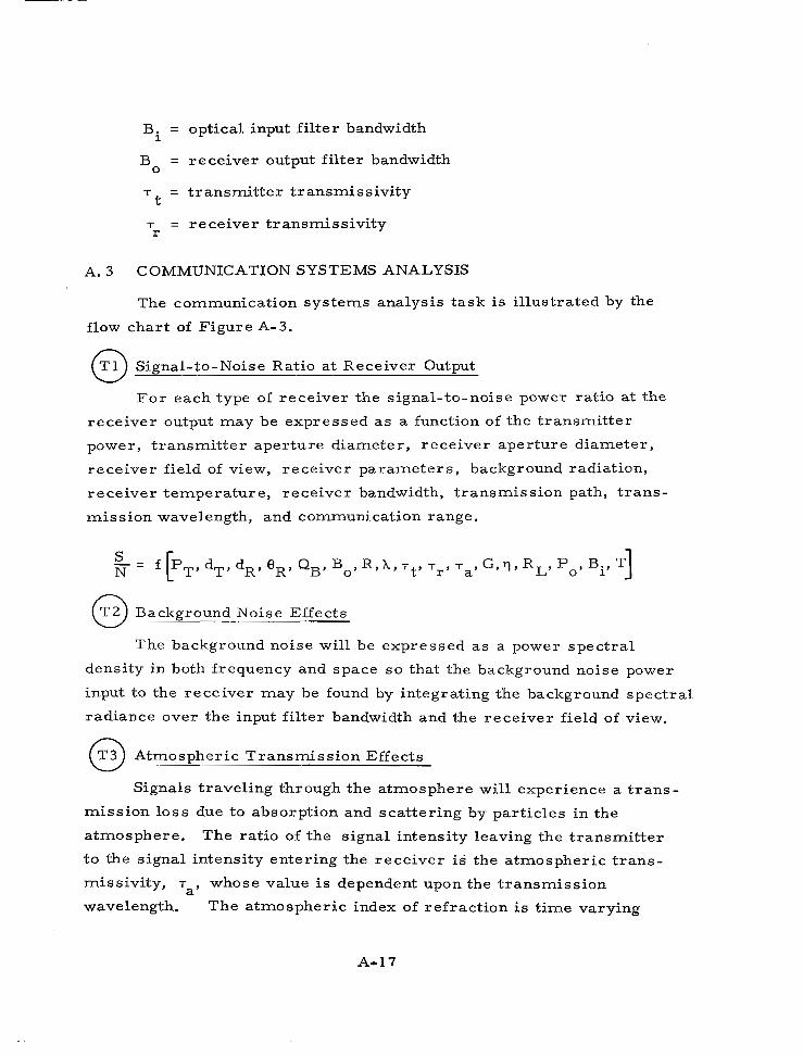
B. = optical input filter bandwidth
Bo = receiver output filter bandwidth
T = t ransmi t te r t ransrn iss iv i ty
T = rece iver t ransmiss iv i ty
1
t
r
A. 3 COMMUNICATION SYSTEMS ANALYSIS
The communication systems analysis task is i l lustrated by the
flow cha r t of F igure A-3.
n (T3) Signal-to-Noise Ratio at Receiver Output
For each type of receiver the signal-to-noise power ratio at the
receiver output may be expressed as a function of the t ransmi t te r
power , t ransmi t te r aper ture d iameter , rece iver aper ture d iameter ,
rece iver f ie ld of view, receiver paralneters, background radiation,
receiver temperature , receiver bandwidth, t ransmission path, t rans-
mission wavelength, and communication range.
0 T2 Background Noise Effects
The background noise will be expressed as a power spectral
density in both frequency and space so that the background noise power
input to the receiver may be found by integrating the background spectral
radiance over the input f i l ter bandwidth and the receiver f ield of view.
0 - T3 Atmospher ic Transmiss ion Ef fec ts
Signals traveling through the atmosphere will experience a t r a n s -
mission loss due to absorpt ion and scat ter ing by par t ic les in the
atmosphere. The ra t io of the s ignal intensi ty leaving the t ransmit ter
to the s ignal intensi ty enter ing the receiver is the a tmospher ic t rans-
missivi ty , T whose value is dependent upon the transmission
wavelength. The atmospheric index of re f rac t ion is t ime varying a’
A-17

because of wind and thermal gradients in the a tmosphere. This causes
a scinti l lat ion effect in which the received signal beam occasionally
moves entirely or partially out of the receiver f ie ld of view. In addi-
tion, changes in the composition of the a tmosphere cause perburba t ions
in the phase f ronts of the t ransmit ted beam, This destroys the spat ia l
coherence of the s ignal and reduces the receiver col lector area over
which heterodyning may be performed. The relationship between
a tmospher ic e f fec ts and th i s coherence a rea is present ly ill defined.
For heterodyne and homodyne detection systems in which spatial
coherence is cri t ical , the effect of the a tmosphere may be descr ibed
by the signal coherence area over which mixing may be performed.
The coherence area l imits the usable s ize of the receiver aper ture .
A. 4 SYSTEMS EVALUATION
The systems evaluat ion task is i l lust rated by the flow chart of
F igure A-4 .
0 El Expres s Signal-to- noise^ Ratio as a Func t ionof Svs t emParamete r s
For each type of receiver the s ignal- to-noise ra t io can be
expres sed i n t e rms of the sys tem parameters .
where
pT -
dT -
'R -
dr =
-
-
-
t ransmit ter power
d iameter of the t ransmit ter antenna
receiver f ie ld of view
d iameter of the receiver antenna
0 E2 Express Sys tem Cos ts as a Function of Sys t em Pa rame te r s
Composite relationships may be developed between the major
system parameters which appear in the s ignal- to-noise ra t io
A-1 8

\
I SIGNAL-TO-NOISE RATIO AT RECEIVER OUTPUT
BACKGROUND NOISE EFFECTS I-@ ATMOSPHERIC TRANSMISSION EFFECTS t-@
Figure A-3. Communication systems analysis flow chart .
EXPRESS SIGNAL-TO-NOISE RATIO AS A FUNCTION OF SYSTEM PARAMETERS
~~~ E l
I 1 ‘1 EXPRESS SYSTEM COSTS AS A FUNCTION OF SYSTEM PARAMETERS
OPTIMIZE SYSTEM COSTS E3
I I , I EVALUATE SYSTEM WEIGHT BURDENS 1
I EVALUATE SYSTEM POWER BURDENS I
I EVALUATE SYSTEM FABRICATION COST BURDENS I
I I
‘N EVALUATE SYSTEM COMPONENT COST BURDENS
EVALUATE SYSTEM COST BURDENS E8
Figure A-4. Systems evaluation flow chart.
A-19

I
expression and the var ious system burdens by manipulation of t he
following set of functional relations.
0 C1 Transmi t te r an tenna cos t
C = KeT(dT) t K K (d,) I t CKT t KSWKT dT dT
0 C2 Receiver antenna cost
m n C = K (dR) t K K (dR) + CKR t KSWKR R
dR eR dR
0 C3 Transmit ter acquis i t ion and t rack system cost
'QT - - 'AT + - (dT) 4T t KS[WBT t K (d,)nT] W~~ d~
0 C4 Receiver acquis i t ion and t rack system cost
0 C5 Transmi t te r cos t
' 'KP + 'KH ' K ~ W ~ ~ ' K ~ W ~ ~
0 C6 Modulation equipment cost
'M - K ~ ~ R ~ - + K K R t CKM t KSWKM
S M B
A- 20

‘ST
0
0
C7 Demodulation equipment cost
‘D - K ~ ~ R ~ + ‘KD ’ K ~ K ~ R ~ ’ K ~ W ~ ~ -
C8 Transmit ter power supply cost
= P S T ’ KSKWsT] [Kp KMRB t K PMWKM t pTt ke K M pQT [wBT
0 C9 Receiver power supply cost
The expressions for @ , @ , and @ , combine to give
a relat ionship between t ransmit ter aper ture diameter and the cost ,
of the transmitter optics and associated tracking equipment which is
dependent upon the transmitter aperture diameter.
cT
CT - - - - KAT(dT)9T t K (dTImT t K K (dT)nT t K nT 0 dT
(dT T
J ”- \ T
fabrication fabrication weight cost weight cost of cost of cost of t r ansmi t t e r t r ansmi t t e r t r ansmi t t e r t r ansmi t t e r an t enna t r acke r t racker antenna
A12 1
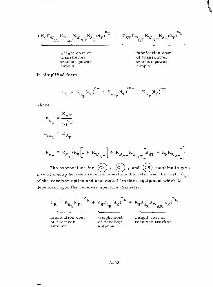
weight cost of t r ansmi t t e r t racker power supply
fabricat ion cost of t r ansmi t t e r t racker power supply
In simplified form
where
KnT KdT lKS [1 KWAT] PaTKWAT - t K P S T ' ]]
WST
The expressions for @ , @ , and @ combine to give
a re la t ionship between receiver aper ture diameter and the cost ,
of the receiver optics and associated tracking equipment which is
dependent upon the receiver aperture diameter.
cR ,
n n CR = K t K K (a,) t K K K - R
eR dR d~ W~~ (dR ) - - -
fabricat ion cost weight cost weight cost of of rece iver of r ece ive r r ece ive r t r acke r antenna antenna
A-22
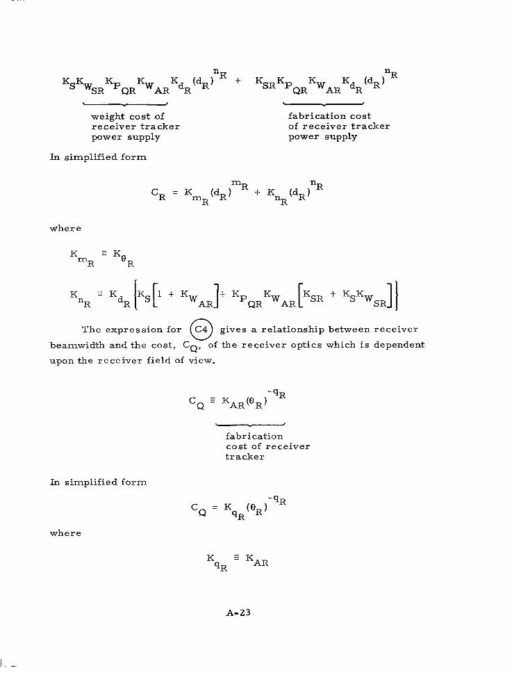
weight cost .of r ece ive r t r acke r power supply
- fabrication cost of r ece ive r t r acke r power supply
In s implif ied form
where
nR ' KdR [ K S [ l t K W AR]+ KPQRKWAR [.SR WSR
The express ion for C4 gives a relationship between receiver 0 beamwidth and the cost, CQ, of the receiver optics which is dependent
upon the receiver f ield of view.
\ * M
fabrication cost of rece iver t r a c k e r
In simplified form
where
A- 23

The expressions for C5 and C 8 combine to give a 0 0 re lat ionship between t ransmit ter power and the cost , CG of the
t ransmit ter and the associated power supply and heat exchanger which
is dependent upon the transmitter power.
K K CG = K (PT)gT + K K (P,) hT t - KST WST
pT wT k e p T t k e pT
” ”
fabrication weight cost of fabrica- weight cost cost of t r ansmi t t e r t i on cos t of t ransmi t te r t r a n s m i t t e r of trans- power supply
mit te r power supply
1 - k + KH( k e)pT ke ) pT
1 - ke
e - - fabrication cost of weight cost of heat heat exchanger exchanger
In simplified form
cG = (pT) + KhT
gT (PTPT t K PT
gT jT
where
K
K [Ks WST + KX ( ie ke)l t -q KST + KH(‘ ”e.) J T e e
A- 24

The expressions for @ , @ , @ , @ , @ a n d
0 C9 combine to give relationships descr ' ibing the f ixed system costs
at the t ransmit ter and receiver which are independent of t he t r ans -
.mitter aper ture , rece iver aper ture , t ransmi t te r power , and rece iver
field of view,
'XT - 'KT + K ~ W ~ ~ + 'AT ' K S W ~ ~ ' 'KP + 'KH ' K S W ~ ~ -
+ K ~ W ~ ~ ' K ~ ~ R ~ ' 'KM t K S M B K R t KSWKM
[ KST t K S K WsT] [KPM K M R B t Kp M WKM t K p~~ W B T ]
K ~ W ~ ~ + 'KE
'XR = CKR t KSWKR t CAR + KSWBR + KFDRB t CKD t KSKDRB
' K ~ W ~ ~ + 'KF
The total system cost is thus composed of a fixed part, which is
not affected by the major system parameters and a var iable par t which
is dependent upon the system parameters.
cs = cv + CXT t CXR
with
cv = CG t CT + c* + CR
where
Cs = to ta l sys tem cos t
Cv = var iab le par t of total system cost (optimization cost)
A-25
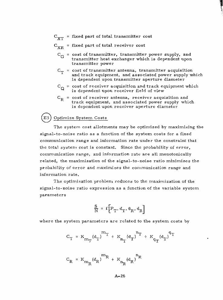
CXT = f ixed par t of to ta l t ransmi t te r cos t
‘XR = f ixed par t of to ta l rece iver cos t
CG = cost of t ransmit ter , t ransmit ter power supply, and t ransmit ter heat exchanger which is dependent upon t ransmit ter power
CT = cost of t ransmit ter antenna, t ransmit ter acquis i t ion and t rack equipment , and associated power supply which is dependent upon t ransmit ter aper ture diameter
C, = cost of receiver acquis i t ion and t rack equipment which
CR = cost of receiver antenna, receiver acquisit ion and
is dependent upon receiver field of view
track equipment, and associated power supply which is dependent upon receiver aperture diameter
0 E3 Optimize System Costs
The system cost a l lotments may be opt imized by maximizing the
s igna l - to-noise ra t io as a function of the sys tem cos ts for a fixed
communication range and information rate under the constraint that
the to ta l sys tem cos t is constant. Since the probability of e r r o r ,
communicat ion range, and information ra te are a l l monotonical ly
re la ted, the maximizat ion of the s ignal- to-noise ra t io minimizes the
probability of e r r o r and maximizes the communication range and
information ra te .
The optimization problem reduces to the maximization of the
s ignal- to-noise ra t io expression as a function of the var iable system
pa rame te r s
- = f P S d 8 N [ T’ T’ R’ dR]
w h e r e t h e s y s t e m p a r a m e t e r s a r e r e l a t e d t o t h e s y s t e m c o s t s b y
m R nR ‘R =
mR -t KnR(dR)
A- 26

CG = K (P,) gT + KhT(PT) hT + K. PT gT J T
under the l inear constraint that the optimization cost remains constant.
If the expressions for the system burdens can be inverted, the resul tant
expressions for the system parameters may be subst i tuted into the
formulation for the signal-to-noise ratio which then may be minimized
by partial differentiation. Appendix A2. 12 d iscusses such a case. If
the system cost expressions are not easi ly invertable , the opt imiza-
t ion must be performed by numerical techniques,
\
By the method of Lagrange mult ipl iers the expression
Q = 6 t A(C, - CT - CR - CG - Ca)
is formed, then the par t ia l der ivat ives of Q with respect to each var i -
ab le sys tem parameter a re se t to zero .
"" aa - 4 3 acR adR adR adR
A" - 0
- = - - A " aa acG apT apT dPT
- 0
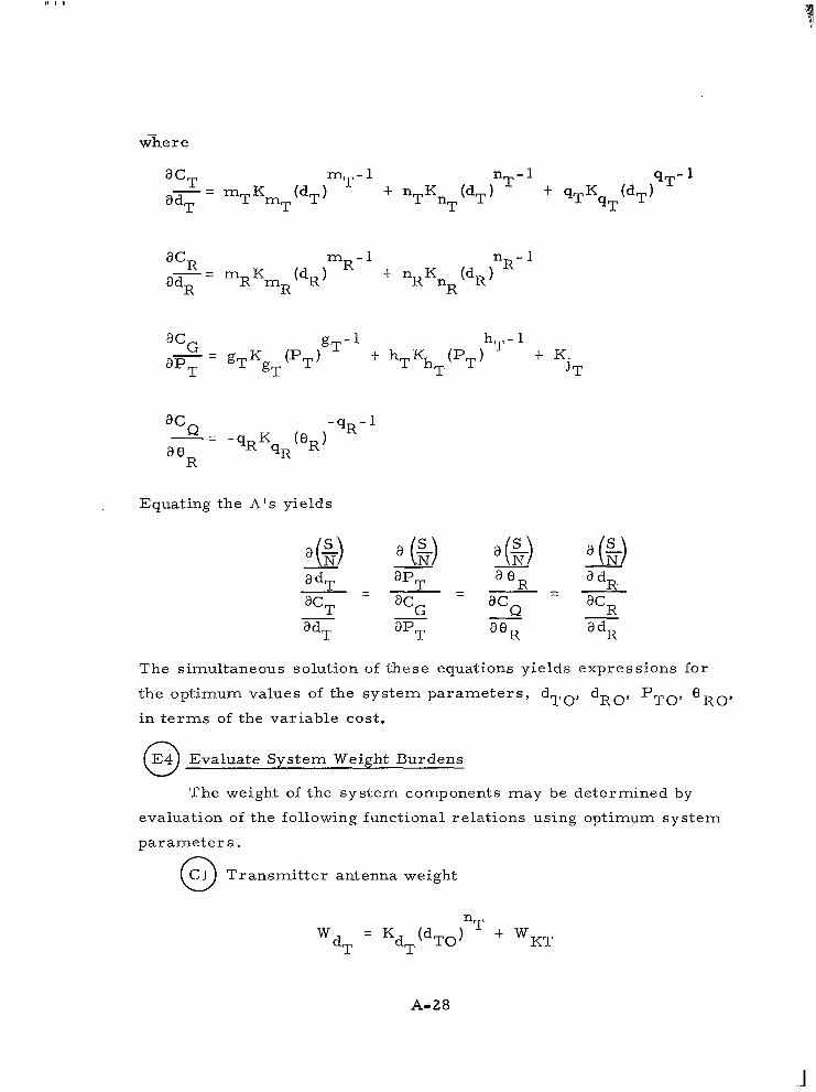
where
mR - 1 - m K (dR)
nR- I
a%- mR nR (’R)
acG - gT- I hT- 1
”
apT gTKgT(PT) (pT)
hT f K.
J T
Equating the A ’ s yields
- adT
5 apT
The simultaneous solution of these equations yields expressions for
the optimum values of t he sys t em pa rame te r s ,
i n t e r m s of the variable cost . dTO’ dRO’ pTO’ ‘RO’
0 E4 Evaluate System Weight Burdens
The weight of the system components may be determined by
evaluation of the following functional relations using optimum system
pa rame te r s .
0 C1 Transmitter antenna weight
A-28

0 C2 Receiver antenna weight
W = K IIR
dR dR ( d ~ ~ ) W~~
0 C3 Transmit ter acquis i t ion and t rack system weight
.QT - - WBT t K (dTo)
W~~ d~~
Receiver acquis i t ion and t rack system weight
WQR = WBR t K ( d R o ) n
W~~ d~~
0 C5 Transmi t t e r and transmitter heat exchanger weight
0 C6 Modulation equipment weight
W M = K R M B ’ W~~
0 C7 Demodulation equipment weight
WD = KDRB t WKD
A-29
L
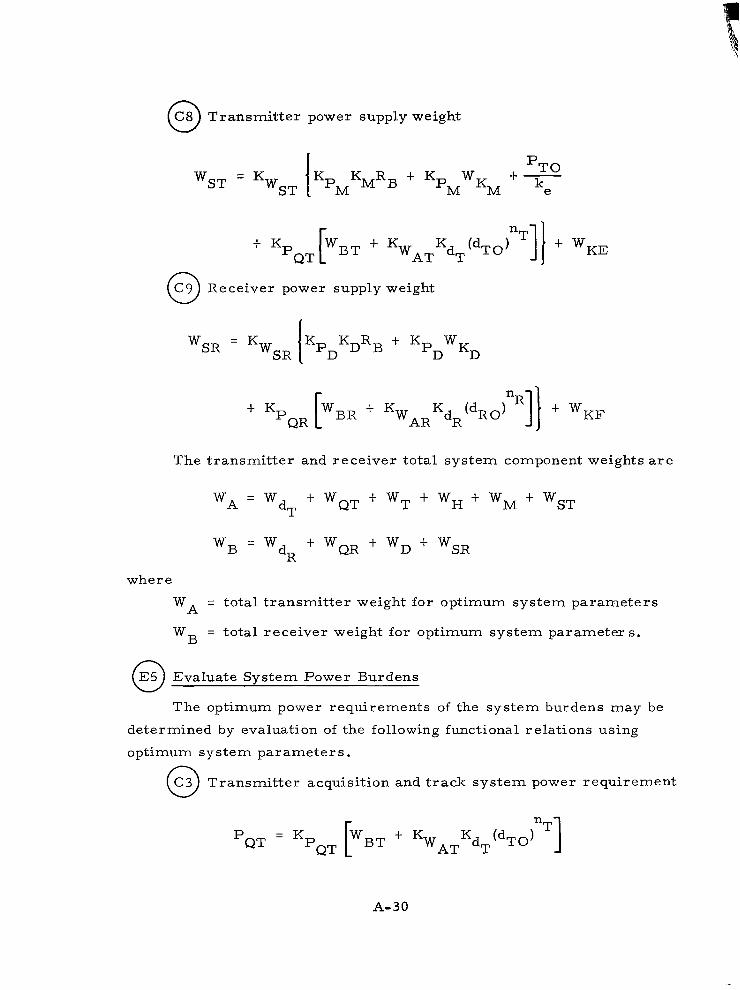
0 C8 Transmitter power supply weight
pTO +- ke
WST = K WST
0 C9 Receiver power supply weight
WSR = K WSR IKPDKDRB ’ pD KD
The t ransmit ter and receiver total system component weights are
WA = w t WQT + WT + WH + WM dT + WST
WB = w dR + w~~ + w~ + W~~
where
WA = to ta l t ransmi t te r weight for op t imum sys tem parameters
W B = total receiver weight for opt imum system parameters .
0 E5 Evaluate System Power Burdens
The optimum power requirements of the system burdens m a y be
determined by evaluation of the following functional relations using
opt imum sys tem parameters .
0 C3 Transmit ter acquis i t ion
P~~ - - KPQT [WBT
and t rack sys tem power requi rement
A-30

0 C4 Receiver acquisit ion and track system power requirement
PQR = K + K WARKdR (dR OTR]
0 C5 Transmit ter power requirement
0 C6 Modulation equipment power requirement
PM = K pM K ~ R ~ + K ~ M W ~ ~
0 C7 Demodulation equipment power requirement
PD = K pD K ~ R ~ ' K ~ D W ~ ~
The t ransmit ter and receiver total power requirements are
PA = PQT + PPT + PM
and
where
PA = total t ransmit ter power requirement for opt imum system
PB = total receiver power requirement for opt imum system
p a r a m e t e r s
p a r a m e t e r s
A-31
I

0
0
E6 Evaluate System Fabricat ion Cost Burdens
The optimum fabrication cost of the system components may be
determined by evaluation of the following functional relations using
opt imum sys tem parameters .
C1 Transmit ter antenna fabr icat ion cost
0 C 2 Receiver antenna fabrication cost
mR C = K eR eR ( d ~ ~ ) ’ ‘KR
0 C3 Transmit ter acquis i t ion and t rack system fabricat ion cost
CNT = CAT t -
Receiver acquis i t ion and t rack system fabricat ion cost
- qR
0 ‘NR = ‘AR ’ K~~ (% 0 )
C5 Transmit ter and t ransmit ter heat exchanger fabr icat ion cost
gT CFL = K pT (pTO) -t ‘KP
1 - k
‘H = k e e)PTO ’ ‘KH
Modulation equipment fabrication cost
- ‘FM - K ~ ~ R ~ ” ‘KM
A-32

and
0 C7 Demodulation equipment fabrication cost
0 C8 Transmitter power supply fabrication cost
pTO KPM M B K R t Kp WKM t -
M ke
[ W , T ' KWAT Kd (dTOp]l " 'KE
0 C9 Receiver power supply fabrication cost
The t ransmi t te r and rece iver to ta l fabr ica t ion costs a r e
CFA = c t CNT t CFL t c t CFM e, H 'FT J.
where
CFA = total t ransmit ter fabr icat ion cost for opt imum
CFB = total receiver fabr icat ion cost for opt imum system
s y s t e m p a r a m e t e r s
pa rame te r s
A-33
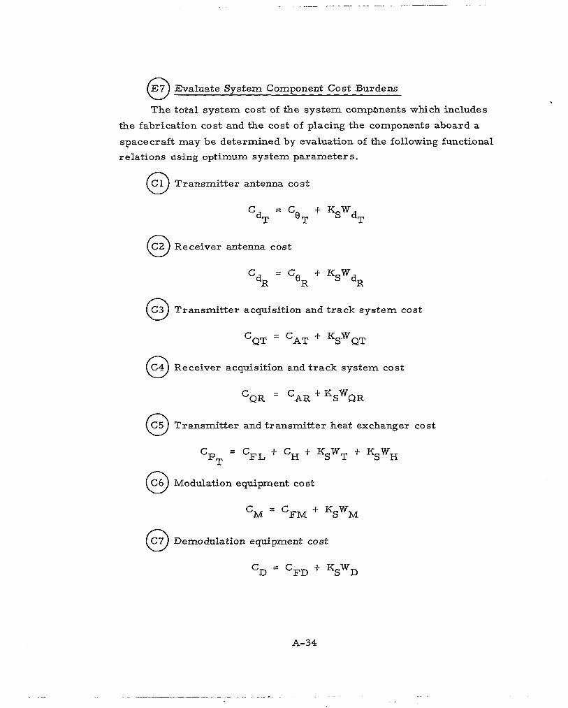
0 E7 Evaluate System Component Cost Burdens
The total system cost of the system compbnents which includes
the fabrication cost and the cost of placing the components aboard a
spacecraft may be determined by evaluation of the following functional
re la t ions us ing op t imum sys tem parameters .
0 C1 Transmit ter antenna cost
cdT = ceT " dT
0 C2 Receiver antenna cost
0 C 3 Transmit ter acquis i t ion and t rack system cost
0 'QT = 'AT + K ~ w ~ ~
C4 Receiver acquis i t ion and t rack system cost
CQR = C~~ + K ~ W ~ ~
0 C5 Transmi t te r and t ransmi t te r hea t exchanger cos t
C = CFL + CH + KsWT f KsWH pT
0 C6 Modulation equipment cost
'M - 'FM + K ~ w ~
0 -
C7 Demodulation equipment cost
A- 34

0 C8 Transmi t t e r
n
power supply cost
'ST = 'FT ' K ~ W ~ ~
Receiver power supply cost
Evaluate System Cost Burdens
The sys tem cos t var iab les for op t imum sys t em pa rame te r s a r e
The var iab le sys tem cos t is then
The to ta l sys tem cos t is
cs = cv t CXT t CXR
The to ta l t ransmi t te r and rece iver cos t s a re
c* = c t c t CXT G T
A-35
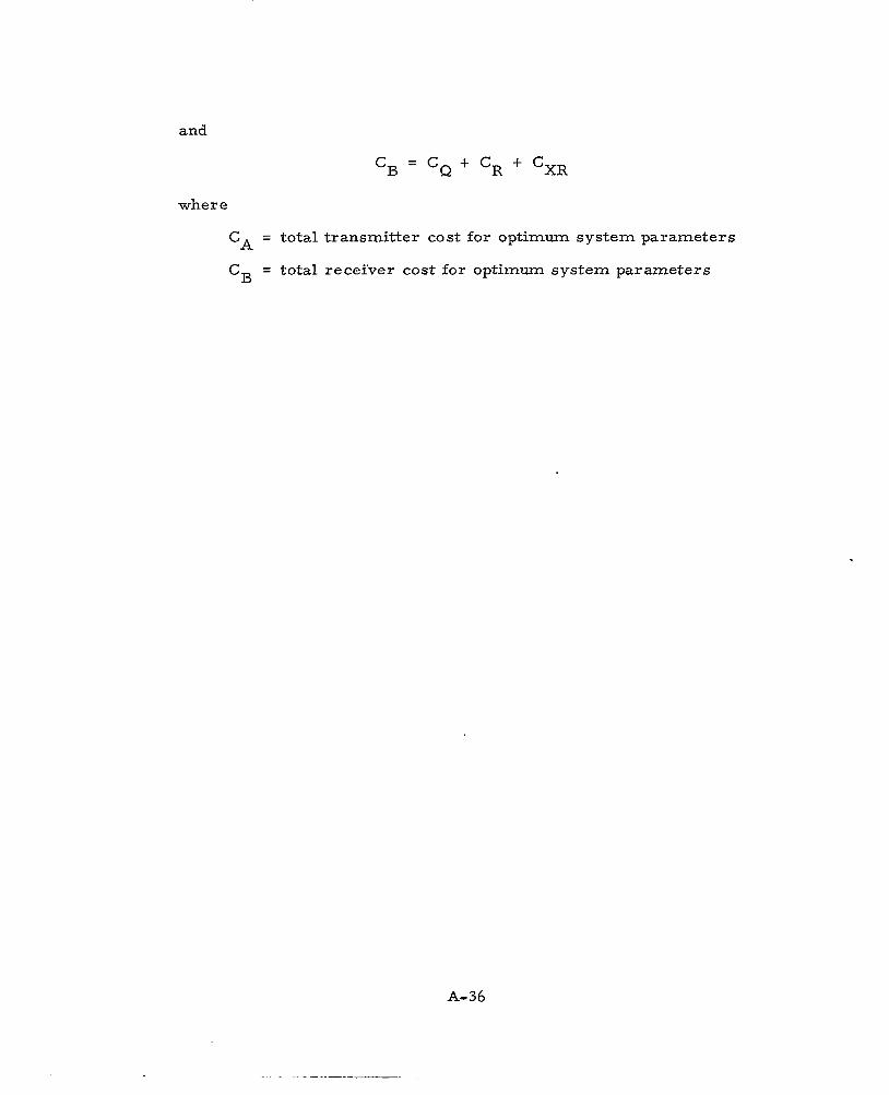
and
CB = c 4- c + CXR Q R
where
CA = total t ransmi t te r cos t for op t imum sys tem parameters
CB = total recei 'ver cost for opt imum system parameters
A-36

APPENDIX B
COPTRAN

"
APPENDIX B
COPTRAN
This appendix is an ex t r ac t f rom a f inal report for NAS 12-566 "Study
and Development of a Mathemat ica l Analys is for the Per formance Assess -
ment of Space Communicat ion System Parameters , ' ' dated May 1969. The
basic work and init ial computer tabulations were done under contract
NAS 5-9637. Subsequently a contract was made between the Hughes Aircraft
Company and NASA-ERC to adapt the original work such that it could be easily
used by a per son not familiar with computer programming. COPTRAN is a
resul t of the contract with NASA -ERG.
A complete documentation of COPTRAN is found in the referenced final
report , Per t inent sect ions are given here which descr ibe what the program
can do and what i s necessary to make it function. A single example i s also
given to indicate the output which may be obtained from the program.
B-1
t .


B. 0 USER'S MANUAL FOR COPTRAN, A METHOD OF OPTIMUM COMMUNICATION SYSTEM DESIGN
B. 1 Introduction
Calculations to determine communication capability of a pulse or digi ta l
, t ransmission l ink are basical ly dependent on a single equation which specifies
the probability of detect ion error for one way t ransmission. While there are
variants in this equation to account for different types of noise, modulation
and demodulation techniques, this one equation documents the interrelation-
ships among the communicat ion system parameters of range , t ransmi t te r
power, antenna gains, noise, etc. In the equation describing the probabili ty
of de t ec t ion e r ro r i t is possible to t rade one system parameter value against
others while maintaining a given performance. Thus, i t is difficult to
determine the "best" combination of pa rame te r s fo r a particular application
although this is an important determination, especially to space missions.
I t i s therefore desirable to formulate an analyt ical method or methodology
of not only select ing parameters which produce the desired performance
within the regulation of the range equation but of selecting optimum param-
eter values which meet the desired performance.
Consider the following relatively simple optimization example for a deep
space communication system. The effective radiated power from a spacecraf t
i s t o be maximized for a specified weight. Now the effective radiated power
may be increased by increasing e i ther the s ize of the transmitt ing antenna or
the t ransmit ter power, or by some suitable combination of i nc reases i n t hese
two parameters . The problem i s to de te rmine the p roper sp l i t in weight
between these two elements to maximize the effective radiated power subject
to the given weight constraint. It is very unlikely that a combination of an
extremely large antenna using a lmost all the available weight with a minimal
t r ansmi t t e r would give the best possible performance, nor would the combina-
tion of an extremely heavy t ransmit ter with a very low-gain antenna. The
optimum configuration probably l ies somewhere between these two ext remes .
In order to determine the opt imum configurat ion, both t ransmit ter power and
antenna gain must be expressed in terms of weight. If these two relationships
a r e known, a straight forward optimization procedure can be employed to
B-3

determine the opt imum values for both t ransmit ter power and the antenna
size associated with the result ing antenna gain.
Such an optimization concept has been expanded to all appl icable param-
eter values in the equat ion descr ibing the probabi l i ty of de t ec t ion e r ro r fo r
both a weight optimization and a cost optimization. The resulting methodology ' has been implemented in a computer program known as COPS (Communication
system Optimization Program with Stops).
The COPS program optimizes the values of the Major Communication
Systems Parameters which are: the t ransmit ter antenna diameter or gain, the
rece iver an tenna d iameter o r ga in , the t ransmi t te r power , and the rece iver
field of view. The program i s implemented for radio frequency homodyne
detect ion systems, opt ical f requency heterodyne detect ion systems, and for
opt ical f requency thermal or shot noise l imited direct detect ion systems.
The COPS program minimizes the total system cost for a g iven t ransmis-
s ion range, information ra te , and probabi l i ty of detect ion error for each
communicat ion system. The total system cost i s a function of the t ransmi t te r
system weight , t ransmit ter system fabricat ion cost , receiver system weight ,
and receiver system fabricat ion cost e i ther s ingly or in any combinat ion.
Fixed values for any of the Major Sys tem Parameters may be en te red in to the
programs. In addi t ion , maximum or min imum parameter va lues , ca l led s tops ,
m a y be placed on each of the Major Sys tem Parameters . The COPS program
provides an output tabulation of optimum values of Ma jo r Sys t em Pa rame te r s
as a function of information ra te .
The inputs required for the COPS program are a tabulation of Sys tems
Physical Data such as: range, sky noise background, wavelength, transmis-
s ivi ty losses , e tc ; System Burdens Data such as : constants re la t ing t ransmit ter
power to weight ; antenna s ize to cost ; e tc . , and System Parameter Constraints
such as the minimum, maximum, or f ixed values for the Major Systems
P a r a m e t e r s .
The COPS program has been wri t ten in Fortran IV language. In order to
facil i tate the use of the COPS program by persons unfamil iar with computer
opera t ion or p rogramming, a buffer computer language called COPTRAN
(Communication system Optimization Program TRANslator) has been developed.
B -4
To operate the COPS optimization program using the COPTRAN language
involves answering a few simple quest ions which are wri t ten in the language
of the user . For instance one quest ion is: "What is the t ransmiss ion range?"
Following this question is a choice of six le t te r mnemonics and the i r mean-
ings. One of these, RANMAR, may be chosen to tell the COPS methodology
through the COPTRAN buffer language that the range (RAN) is a M a r s (MAR) dis tance, lo8 km. Similar s imple quest ions, again using a multiple choice
l ist ing of mnemonics , a re answered for such top ics as the modulation type,
the type of optimization desired, the type of output desired, e tc . The user
may a l so use s tandard se t s of data for the interrelat ionship of t r ansmi t t e r
cost to power, e tc . (burden re la t ionships) . Or the user m a y change one or
all the nominal constants, thus superceding the stored values.
The mnemonic instruct ions and data values that are selected by the user
to descr ibe the p roblem he wishes to so lve a re wr i t ten down by the user on a
simple COPTRAN form. This form is then used as a guide to punch computer
cards , one card per mnemonic o r da ta va lue . The cards become par t of the
COPTRAN program and are batch processed by a computer. The computer
resu l t s a re re turned to the user e i ther in a l ine printout or in Cal Comp plots.
Figure B-1 summarizes the s teps used to obtain opt imized communicat ions
parameters us ing the COPS computer program with the COPTRAN language.
The major sect ions of the COPTRAN User's Manual which follow, are
summarized briefly for convenience.
Section B. 2 - COPTRAN Programming Structure
The COPTRAN program has several par ts , some of these a re changed by
the user and some a re no t in the course of solving a problem. This section
contains a descr ipt ion of these par t s , def ines the t e rms used to descr ibe them
and indicates which parts are changed by the user when solving a problem.
Section B. 3 - COPTRAN Program Entry
S imple forms for p roblem en t ry a re p rovided to a id the user in descr ib ing
his p rob lem in COPTMN l anguage . The fo rms a r e marked to indicate where
the symbols are placed and where the numerical value for the data is placed.
B -5

USER AND HIS REQUIREMENTS
CARDS FUNCHED FROM COPTRAN CODING
r
PROGRAM RUN BY COMPUTER
USER F U T S HIS REQUIREMENTS ON COPTRAN SHEETS
S A M
USER'S PROBLEM IS ASSEMBLED AS A CARD DECK
OUTKIT RETURNED TO USER
F i g u r e B- 1. C O P T R A N P r o g r a m m i n g
B-6

The program en t ry p rocedure needed for a computer faci l i ty using the
IBM 7094/IBSYS or the GE 635/GECOS III is also given.
Section B. 4 - COPTRAN Use
This section i s the one used by the user 's to put his problem in COPTRAN
language. The user considers each of the several categories and enters
mnemonics on the COPTRAN forms (see Sect ion 4 . 3) as appropriate. Section
4 . 4 is complete, containing all of the COPTRAN mnemonic values.
Section B. 5 - COPTRAN Use Simplified
The s implif ied vers ion of COPTRAN does not provide all the flexibility of
the general program. As such it l imits the problems that may be solved. I ts
advantage is it allows a user to obtain optimized solutions without the general
program complexity.
Section B. 6 - COPTRAN Examples
Seven examples are given in COPTRAN solutions. These examples have
been designed to indicate the capabilities of COPTRAN by using i t s var ious
features .
All program solutions published except Example E have been obtained from
the IBM 7094/IBSYS computer and verified on the GE 635/GECOS III computer.
The published solution for Example E has been obtained from the GE 635/
GECOS III computer.
Section B. 7 - COPTRAN Multiple Case
COPTRAN multiple case subprograms include the "Increment" subprogram,
the "Repeat" subprogram, the "Worth" subprogram and the "New Set" subpro-
gram. These are br ief ly descr ibed in Sect ionB. 4 , COPTRAN Use, but are
given in further detail here.
SectionB. 8 - COPTRAN E r r o r M e s s a g e s
The use of e r ror messages i s no ted in Sec t ion B. 4. The ac tua l messages
a r e given.
B -7

Section B. 9 - COPTRAN Automatic Data Selection
Mapy values used in the COPTRAN optimum solutions are taken f rom data
storage. This section l ists the values used and the conditions under which
they become par t of the COPTRAN program.
Section B. 10 - COPTRAN Nominal Value Decks
The mnemonics selected by the u s e r o r by the COPTRAN program in
turn select numerical values for a large number of constants (e. g . , t hose
relating transmitter power to weight) used in a given solution. The numerical
values a r e l is ted in this sect ion. Also given are means for changing o r adding
to the data storage.
B -8

B. 2 ' COPTRAN St ruc ture
B. 2. 1 Introduction. - The COPTRAN programming language is a special-
ized, simple computer language used in the design of communication systems.
COPTRAN allows a user to ,determine the optimum configuration of a complex
communication system with relatively few instructions phrased in the context
of his problem and without the necessity of supplying large quantities of data
to the computer . This is accomplished by s tor ing nominal values of the p ro-
gram da ta in the computer da ta banks . The per t inent da ta for a par t icu lar
problem is then automatically fetched by the COPTRAN program unless
countermanded by par t icular user select ions.
A COPTRAN job is composed of six main par ts which are subdivided as
follows:
COPTRAN Control Program
COPS Program
Output Program Program
Nominal Value Data
COPTRAN System
COPTRAN Instructions
COPTRAN Data COPTRAN User Program
The f i r s t four par t s of a COPTRAN job comprise the COPTRAN System Pro-
gram. This program is configured for a par t icular computer instal la t ion; i t i s
not changed by the general user . The las t two p a r t s of a COPTRAN job a r e
the COPTRAN User Program, which is wri t ten by the user for each problem.
This manual is la rge ly a descr ipt ion of the COPTRAN User Program.
Table B-I summarizes the nomenclature for the COPTRAN s t ructure while
Table B -11 gives the COPTRAN programming nomenclature used in this manual.
The following two parts of this sect ion descr ibes the basic use of COPTRAN
instructions and COPTRAN data, which are the user supplied parts of a
COPTRAN job.
B-9

TABLE B-I COPTRAN STRUCTURE NOMENCLATURE
COPTRAN System P r o g r a m
COPTRAN Control P r o g r a m
COPS Program
Output Program
Nominal Value Data
COPTRAN
COPTRAN Instructions
COPTRAN Data
The COPTRAN System Program i s composed of FORTRAN IV programming language state- ments and is in four basic par ts : 1 ) the COPTRAN Control Program, 2 ) the COPS P r o g r a m , 3 ) the Output Program, and 4) the Nominal Value Data. The COPTRAN System Program may be in e i ther FORTRAN source or object format for a par t icu lar computer installation.
A program which decodes the COPTRAN User Program instruct ions and provides l inkages between COPTRAN System Programs.
A program which provides opt imum values of system parameters and evaluat ion of associated cost , weight, and power burdens of a communication system as a function of information ra te .
A program which controls the format and presentation of output tabulations and plots.
L i s t s of System Physical Data , System Burdens Data , and System Parameter Con- straints Data from which automatic selections a r e m a d e .
A U s e r P r o g r a m l i s t of instruction mnemonics and data entries which automatically provides information for the performance of the COPS program.
L i s t s of mnemonics selected by the user to descr ibe his problem, the method of opt imiza- tion, and the presentation of the resul ts .
COPTRAN Data selected by the user to incorporate individual burdens, physical data, and parameter contraints into the COPTRAN solution.
B-10

TABLE B-I1 COPTRAN PROGRAMMING NOMENCLATURE
Job
Case
Run
Instruction/data s e t
Instruction/data category
. - ". . . ..
That which is submittal to the computer. I t cons is t s of a COPTRAN System Program, a COPTRAN User Program, and whatever submittal information is required by a com- pute r ins ta l la t ion.
A single solution of optimization equations by COPS program.
The resu l t s of one or more cases obtained by repeated performance of COPS program under direction of the increment o r repea t subpro- g r a m s o r t h e new instruct ion/data set .
A list of COPTRAN instruction mnemonics and da ta en t r ies .
A grouping of re la ted instruct ions or data en t r i e s . . ~ ~~ ~~~
B. 2 . 2 COPTRAN Instructions. - COPTRAN instructions are single
mnemonics which describe the communication problem to be solved, the
method of optimization, and the presentation of resul ts . The instruct ions
are divided into the following five classifications.
1. Physical Environment, which includes:
2 .
Transmit ter locat ion (spacecraf t )
Receiver location (earth)
Transmission range (one of a s e t of selected ranges may be chosen
to indicate physical environment or another range choice may be
made and the environment specified)
Background (choice of phys ica l source of background radiation)
Communication System, which includes:
Transmission wavelength (one selected wavelength may be chosen)
Modulation and demodulation methods (choice of one of s e v e r a l s e t s
available).
B-11

3. Optimization Basis, which includes:
Weight / fabr icat ion cost opt imizat ion: ( t ransmit ter system weight ,
t ransmi t te r sys tem fabr ica t ion cos t , rece iver sys tem weight , and
receiver system fabricat ion cost may be minimized individually or in
any combination).
Antenna Parameter Opt imiza t ion : (Transmi t te r an tenna ga in o r
diameter and receiver antenna gain or diameter may be opt imized) .
4 . Processing, which includes:
Computation format (choice of init ial and f inal values of information
rate and number of information ra te data points calculated) .
Pr int format (choice of data and results to be printed in tabular form).
Plot format (choice of results to be plotted by Cal Comp plotter) .
5. Nominal System Burdens" (see Section B. 10 for descr ipt ion)
Choices of system burdens may be made from a data bank list i f auto-
mat ic select ions are not desired. (Sect ion B. 9 descr ibes au tomat ic
data selection. ) System burdens va lues may a l so be en te red as new
data i f de s i r ed .
B. 2 . 3 COPTRAN Data. - COPTRAN data is the means by which individual
burdens , phys ica l da ta , and parameter cons t ra in ts a re inser ted in to the
COPTRAN User Program. If the automatic burdens and physical data selec-
tions provided by the COPTRAN instructions are acceptable to the user, and no
parameter cons t ra in ts a re spec i f ied , there w i l l be no COPTRAN Data for the
COPTRAN User Program. The COPTRAN User Program has been developed
so that user supplied COPTRAN Data automatically replaces i tems of data
normally selected f rom data banks. The program data is of three types.
.C -6.
Burdens represent the modeled re la t ionship between system parameters and the weight, fabrication cost , and power requirement of a component. For example, the transmitter system weight, Wx, may be modeled in terms of the t ransmit ter power, PT as Wx = K w T ( P T ) ~ T + WKP where KW hT, and WKp a re bu rden cons t an t s . TY
B- 12

1 . System Physical Data
Phys ica l da ta such as s igna l - to-noise ra t io , a tmospher ic t ransmiss i -
vi ty , receiver temperature , e tc .
2 . System Burdens Data ~
Weight, fabrication cost , and power requirement burdens for com-
munication system components.
3. System Parameter Cons t ra in ts
These a re f ixed and s top va lues of the Major Communication System
P a r a m e t e r s , namely t ransmit t ing or receiving antenna gains or
diameters , t ransmit ter power, and receiver f ie ld of view. (A Ilfixed'l
parameter value is one that remains f ixed throughout all port ions of
the optimization. A "stop" in the parameter value is the minimum or
maximum va lue the parameter may take . For ins tance , a communica-
t ion problem may require a fixed antenna diameter for a receiving
antenna on ea r th of 64 meters and have a stop value for a space
antenna diameter of 10 meters . The op t imiza t ion program w i l l
determine the optimum spli t between the spacecraft antenna size and
spacecraf t power as a function of da ta ra te . A s the data ra te require-
ments increase , the t ransmi t te r power and t ransmi t t ing an tenna s ize
w i l l increase unti l the antenna size of 10 m e t e r s is reached . For
larger data ra tes , the antenna s ize w i l l r ema in a t 10 meters and the
t ransmit ter power w i l l i nc rease , at a f a s t e r r a t e now, to meet the
demands of higher data ra tes . )
R- 13

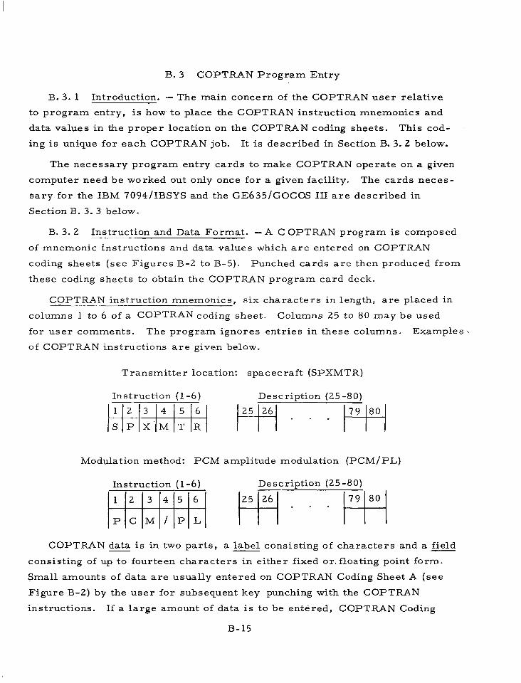
B. 3 COPTRAN Program Entry
B. 3 . 1 Introduction. - The main concern of the COPTRAN user relative.
to p rogram en t ry , is how to place the COPTRAN instruction mnemonics and
data values in the proper location on the COPTRAN coding sheets. This cod-
ing is unique for each COPTRAN job. It is described in Section B. 3. 2 below.
The necessary program entry cards to make COPTRAN operate on a given
computer need be worked out only once for a given faci l i ty . The cards neces-
sary for the IBM 7094/IBSYS and the GE635/GOCOS I11 a re desc r ibed i n
Section B. 3 . 3 below.
B. 3 . 2 Instruction ~" and Data Format . -A C OPTRAN program is composed
of mnemonic instructions and data values which are entered on COPTRAN
coding sheets (see Figures B-2 to B-5). Punched cards are then produced from
these coding sheets to obtain the COPTRAN program card deck.
COPTRAN - ~~ instruction mnemonics, six characters in length, are placed in
columns 1 to 6 of a COPTRAN coding sheet. Columns 25 to 80 may be used
for user comments . The program ignores entr ies in these columns. Examples '
of COPTRAN instructions are given below.
" -.
Transmitter location: spacecraft (SPXMTR)
Instruction (1 -6) Description (25-80)
1 1 2 3 4 5 6
I S R T X ' M P
Modulation method: PCM amplitude modulation (PCM/PL)
Instruction (1 -6) Description (25-80)
COPTRAN data is in two parts, a label consis t ing of characters and a field - consisting of up to fourteen characters in e i ther f ixed or . f loat ing point form.
Small amounts of da ta a re usua l ly en te red on COPTRAN Coding Sheet A ( see
F igure B-2) by the user for subsequent key punching with the COPTRAN
instruct ions. If a large amount of data is to be entered, COPTRAN Coding
B- 15

Sheets By Cy and D shown in Figures B - 3 and B-5 respectively may be
uti l ized. These later coding sheets contain preprinted data labels. Each
da ta parameter w i l l be punched on a s ingle card.
The data label must be justif ied left in columns 1 to 6 on the coding sheet.
Columns 7, 8, 23 , and 24 are left blank. The data value is entered in columns
9 to 22. Columns 2 5 to 80 may be employed for users comments.
Examples of fixed and floating point entries in the data field are given below.
The decimal point in both cases is always i n column 14. For floating point
numbers the l e t te r E must appear in column 19 followed by the sign (f) i n column 20. The exponent must be justified right to column 22.
B- 16

*E
N
4 Nl -
4- T 4 4
B- 17

COPTRAN CODING SHEET A
NAME DATE PROBLEM
COJPPTRAN INSTRUCTIONS AND DATA
Figure B-2 . COPTRAN Coding Sheet A

COPTRAN CODING SHEET B
NAME DATE PROBLEM
COPTRAN INSTRUCTIONS AND DATA E
2 3 4 6 a f7 8 s10111zh31~~6l61~18"i~~z1nn24~
1 2 3 4 5 6 7 8 01011121314~15101718192021222324
Figure B - 3 . COPTRAN Coding Sheet B

COPTRAN CODING SHEET c
NAME DATE PROBLEM
td N 0
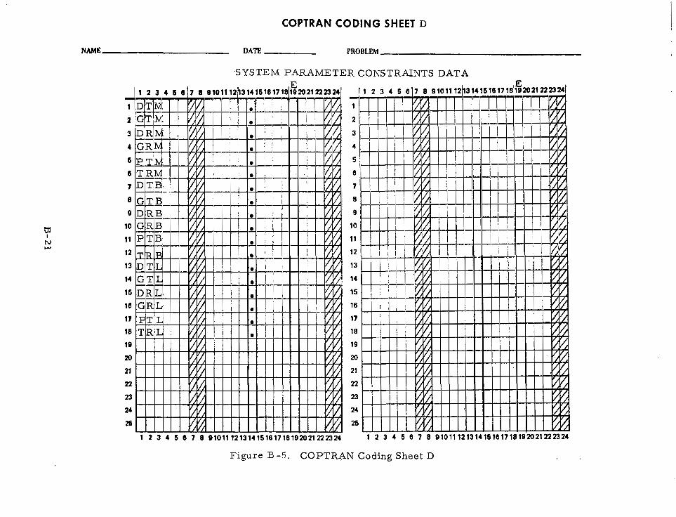
COPTRAN CODING SHEET D
NAME

B. 3. 3 Job En t rv fo r Compute r In s t a l l a t ions . - The COPTRAN job c a r d
deck cons i s t s of t h e C O P T R A N S y s t e m P r o g r a m c a r d d e c k , t h e C O P T R A N
U s e r P r o g r a m c a r d d e c k , a n d a n y s u b m i t t a l c o n t r o l c a r d s r e q u i r e d f o r a
p a r t i c u l a r c o m p u t e r i n s t a l l a t i o n . T h e C O P T R A N S y s t e m P r o g r a m c a r d d e c k
should no t be a l te red by t h e g e n e r a l u s e r . C O P T R A N j o b d e c k s t r u c t u r e s f o r
an IBM 7094/IBSYS and a G E 635/GECOS 111 computer ins ta l la t ion a re shown
in F igu res B-6 and B-7 . The submi t ta l cont ro l cards requi red for these
in s t a l l a t ions a r e i den t i f i ed by a ' I $' I i n c a r d c o l u m n 1.
As present ly implemented COPTRAN on the IBM 7094/IBSYS Version 13
computer ins ta l la t ion does no t execute the Nor th Subprogram due to memory ( 2
l imi ta t ions . The G E 635/GECOS III compute r i n s t a l l a t ion p rov ides a l l of the
COPTRAN fea tures .
7/8 PUNCH-END OF FILE CARD
EXECUTE IB JOB CARD
$ JOB CARD FOR USE IN INSTALLATION ACCOUNTING
F i g u r e B - 6 . COPTRAN Job Deck S t r u c t u r e f o r a n IBM 7 094 /IBSY S Ve r s ion 1 3 Computer
Ins ta l la t ion
B-22

ENDJOB CARD-PHYSICALLY LAST CARD IN DECK: NOTE: THE OPERATIONS STAFF OF 5 ENDJOB A PARTICULAR FACILITY
CHARACTER SET CARD-IDENTIFIES MORE SPECIFIC INFORMATION THE CHARACTER SET USED: ON CONTROL CARDS. $ I NCODE IBMF (INDICATED BY: $) (THIS INDICATES THAT THE IBM FORTRAN CHARACTER SET IS USED)
SHOULD BE CONTACTED FOR
LIMITS CARD-SPECIFIES
SIZE, AND LINES OF OUTPUT FOR THIS MAXIMUM EXECUTION TIME, MEMORY
\ I LIMITS IO, 15000, ,5000 I IDENT
EXECUTION CARD-LOADS THE
I EXECUTE I SNUMB COPTRAN SYSTEM FOR EXECUTION:
IDENTIFICATION CARD-CONTAINS ACCOUNTING
S IDENT O06,56815,3314A,61403,J A DOE INFORMATION:
SEQUENCE CARD-CONTAINS THE SEQUENCE NUMBER FOR THIS JOB: $ SNUMB C4400
F i g u r e B-7. C O P T R A N Job Deck S t ruc tu re fo r a G E 635/GECOS I11 Computer Instal la t ion
B- 2 3

B. 4 COPTRAN Use - A Complete Listing of COPTRAN Instructions and Data Mnemonics
This section contains a complete listing of COPTRAN instruction and data
mnemonics including a brief description of all of the COPTRAN subprograms.
In order to specify a problem properly the user must consider each COPTRAN "
category sequent ia l ly . In some instances several ins t ruct ions o r data entries
must be selected in each category. The notes associated with each category
indicate the restrictions that must be observed.
The user ' s a t ten t ion is called to: Section B. 5, which describes a s impli-
f ied version of COPTRAN use. A version that does not require consideration
of the subprograms (Increment, Repeat, Worth, etc. ), but does provide com-
plete optimization; to Section B. 6 whichgive examples of COPTRAN use; and
to SectionB. 7 which describes the multiple case subprograms in greater detail .
The categories and their titles are as follows:
Category
1 Transmit ter Locat ion 2 Receiver Location 3 Transmission Range 4 Background 5 Transmission Wavelength 6 Modulation and Demodulation Methods 7 Optimization Basis 8 Computational Format 9 Case Title
10 P r i n t F o r m a t 11 P lo t Format
*12 Worth Subprogram 13 Nominal System Burdens 14 System Physical Data 15 System Burdens Data 16 System Parameter Constraints Data 17 Increment Subprogram 18 P r o c e s s 19 Repeat Subprogram 20 New Set 2 1 End of Run
*Not presently implemented on the IBM 7094/IBSYS Version 1 3 computer installation.
B- 2 5

Complete Listing of COPTRAN Instruction and Data Mnemonics
Note: 1. Circled entr ies indicate instruct ion and date categories
t h a t m u s t be suppl ied for every COPTRAN User Program
2. Descriptions of instructions and data in columns 25 to 80
may be changed or omitted without affecting program.
Category Transmit ter Locat ion (Choose only one)
1 Note: If no choice is made , p rogram se lec ts SPXMTR
instruction.
Instruction (1 -6)'" Description (25-80) .L .L
SPXMTR-~ Spacec ra f t t r ansmi t t e r -~ - , "~ -
Category Receiver Location (Choose only one)
I 2 Note: If no choice is made , p rog ram se l ec t s EARCVR
instruction.
Instruction (1 -6) Description (25-80) .VI .VI
EA R c v R" "- Ear th r ece ive r ~~~
*Indicates column numbers, see Section B. 3. 2. **If Ear th t ransmi t te r and/or space rece iver a re des i red , these mnemonics
may be used and appropriate changes can be made using categories 13, 14, 15.
B- 26
Category Transmission Range (Choose only one)
1 @ Note: 1. If no choice is made , p rog ram p r in t s an e r ro r
message and proceeds to next case specif ied by
NEWSET (see Category 20) instruction.
2. If RANOTH instruction is selected, range value
must be included w i t h COPTRAN data in Category
14 statement. In addition, power supply burdens
in Category 1 3 a n d / o r 15 statements indicated by
dagger ( t) that are affected by range must be
supplied. Failure to comply with this rule causes
an error message to be pr inted. The program
then proceeds to next case specified by NEWSET
(see Category 2 0 ) instruction.
Instruction (1 - 6 ) Description (25-80) RANMAR Mars range (1. 0 E t 13 cm)
RAN JW Jupi ter range (7. 5 E t 13 cm)
RANSAT Synchronous satellite range (3. 6 E + 9 c m )
R A N ~ T H * Other range value
Category Background (Choose only one)
@ Note: If no choice is made , p rog ram p r in t s an e r ro r mes -
sage and proceeds to next case specified by N E W -
SET (see Category 2 0 ) instruction.
Instruction (1 - 6 ) Description (25-80)
BKDSKY Day sky ( for opt ical t ransmission)
BKNSKY Night sky (for optical transmission)
BKGALT Galactic (for radio transmission)
-“If des i red , RANMAR, RANJUP o r RANSAT m a y be chosen in order to select burdens per t inent to these general ranges and then specify the exact range by use of the RANG data value change (see Category 14).
B- 27

0 ~~ ~
Category Transmission Wavelength (Choose only one)
Note: 1. If no choice is made , p rogram pr in ts an
e r ror message and proceeds to next
case specified by N E W S E T (see Category 20)
instruction. i 2. If LAMaTH instruction is selected, the
following must also be done: (a) the
wavelength value must be included with
COPTRAN data in Category 14 statement,
(b) system physical d a t a in Category 1 3
and /or 1 5 s ta tements indicated by as ter isk
(:::) that are affected by wavelength must
be supplied. (c) stop values must be
supplied for the non-fixed maximum and
minimum values of the four major system
pa rame te r s ( s ee F igu re B -5 and see
Category 16) . Failure to comply with
these rules c a u s e s a n e r r o r m e s s a g e t o
be pr inted, The program then proceeds
to next case specified by NEWSET (see
Category 20) instruction.
Instruction (1 -6) Description (25-80)
LAM05 1 X = 0. 51 micron
LAM084 X = 0. 84 mic ron
LAM 1 06 X = IO. 6 mic rons
LAM13C X = 13 cm (2. 3 GHz)
L A M ~ T H * Other wavelength value
*If desired, LAM051, LAM084, LAM06 or LAM13C may be chosen in order to select burdens per t inent to these general f requencies and then specify the exact frequency by use of the LMDA data value change (see Category 14. )
B- 28

Category Modulation and Demodulation Methods (Choose only one
8 modulation and demodulation - pa i r )
Note: 1 . If no choice is m a d e p r o g r a m p r i n t s a n e r r o r
message and proceeds to next case specified
byNEWSET (see Category 20) instruct ion.
2. Sys tems burdens a re ava i lab le for au tomat ic
data selection only for those modulation and
demodulation methods indicated by "available"
in the table below. If any other select ions of
modulation and demodulation methods are made
sys tem burdens in Category 13 and/or 15 s ta te -
ments must be supplied. Shaded squares in the
table below indicate that modulation and demodu-
lation methods are not compatible with transmis-
sion frequency. Failure to comply with this rule
c a u s e s a n e r r o r m e s s a g e t o be printed. The pro-
gram then proceeds to next case specified by
NEWSET (see Category 20) instruct ion.
System Burdens Availabil i ty
Modulation Demodulation
Method
PCM/AM
GP TDIR . ~ .. .
P C M / P S
~ P T D I R
PCM/PL
OPTDIR
PCM/FM
. - ~ ~~~
QPTHET
PCM/PM
RADH(PM
Transmission Wavelength .. . - - . .
x = .o. 51 x = 0 . 84 1 = 10.. 6 mic ron mic ron mic ron X = 1 3 c m
not currently not currently available available I available I available not current ly not current ly
available I available I available
available
B- 29

I II II I I
Instruction (1 -6)
1 1 I I
PCM/AM
~ P T D I R
PCM/PL
~ P T D I R
PCM/ FM
~ P T H E T
PCM/PM
R A D H ~ M
P C M / P S
~ P T D I R
Descript ion (25-80)
PCM amplitude modulation
Optical direct detection
PCM polarization modulation
Optical d i rect detect ion
PCM frequency modulation
Optical heterodyne detection
PCM phase modulation
Radio homodyne detection
P C M pulse shift modulation
Optical direct detection
B-30
Category Optimizat ion Basis (Choose f rom e ,ach of the two
0 subcategories)
Note: If indicated choices are not made, program pr ints
an e r ror message and proceeds to next case spec i -
fied by NEWSET (see Category 20) instruction.
7a Weight/Fabrication Cost Optimization (Choose' at
least one; mult iple choices provide joint
optimization. )
Instruction (1 -6) Description (25-80)
X M W T ~ P Transmit ter weight opt imizat ion
R C W T ~ P Receiver weight optimization
X M F C ~ P Transmit ter fabr icat ion cost opt imizat ion
R C F C ~ P Receiver fabrication cost optimization
Note: If r e c e i v e r p a r a m e t e r s d R o r G R and 8, o r t r a n s -
m i t t e r p a r a m e t e r s d T o r G T and PT a r e not to be
optimized in weight or fabrication cost , their f ixed
values must be given in Category 15 statement.
Selection of more than one instruction in this sub-
category provides joint optimization of burdens (i. e. , fabricat ion cost or weight) se lected.
7b Antenna Parameter Optimization (Choose only one
a s indicated)
Instruction (1 -6) D T D R ~ P
G T D R ~ P
D T G R ~ P
G T G R ~ P
Note: 1.
Description (25-80)
Transmit ter antenna diam. and receiver antenna diam. opt. Transmitter antenna gain and receiver antenna diam. opt.
Transmit ter antenna diam. and receiver antenna gain opt.
Transmitter antenna gain and receiver antenna gain opt.
T ransmi t t e r o r r ece ive r an t enna ga in op t imiza - tion is to be used only for radio frequency sys t ems . If no choice is made, DTDRGP is automatically selected.
.
B-31

Category Computation Format (Choose one of each)
8 Note: 1.
2.
Instruction (1 -6)
If no choice is made , p rog ram se l ec t s RBINTO,
RBFIN9, RBFRQ2 instructions.
Final information rate, RB, mus t be g r e a t e r
than ini t ia l information ra te . Fai lure to com-
p ly wi th th i s ru le causes an e r ror message to
be pr inted. The program then proceeds to next
case specified by NEWSET (see Category 20)
instruction.
Description (25-80)
RBINT - Init ial information rate
RBFIN - Final information ra te
RBFRQ - Number of computations per decade
Initial Information Rate Instructions
I RBINTO RBINT 1 RBINT 2 RBINT 3 RBINT4
I R~ = 105 RB = l o 6 RB = 1 0 7 RB = l o 8 I Final Information Rate Instruction
I RBFIN1 RBFIN2 RBFIN3 RBFIN4 RBFIN5
I 1 RB = 10 RB = 10 2 RB = 10 3 RB = 10 4 5 RB = 10
I B R = 10 R = 1 0 RB = 1 0 RB = 1 0 6 7 8 B
B-32

. ... . . .. . .
Number of Computations per Decade Instruction I
Category Case Tit le (Choose i f de s i r ed )
9
-~ Instruction (1 -6) Description (25-80)
TITLEE (Ti t le to be pr inted on tabulation and plots f o r
each ins t ruc t ion lda ta se t . ) -- . - ~ " ~
I .

10 Note: 1. If no choice is made , p rog ram se l ec t s PRTALL
2
Instruct ion (1 -6)
PRTBUR
PRTSPD
PRTSNC
PRTBRC
PRTSPC
P R T ~ P T
PRTWGT
PRTPWP
PRTFAB
PRTSYC
PRTALL
PRTDAT
PRTWTH
Category Pr in t Format (Choose ins t ruc t ions des i red)
-
instruction.
See Worth subprogram, Section 4 . 7 . 4 , desc r ip -
t ion for fur ther information on PRTWTH
instruction.
Descr ipt ion (24-80)
Pr in t sys tem burdens da ta
Pr in t sys tem phys ica l da ta
Pr int s ignal- to-noise ra t io constants
Pr in t sys tem burden cons tan ts
P r in t pa rame te r cons t r a in t s
P r in t op t imum sys t em pa rame te r s
Print weight burdens for opt. system
p a r a m e t e r s
Pr int power burdens for opt . system
p a r a m e t e r s
Pr int fab cost burdens for opt . system
p a r a m e t e r s
Pr int system cost burdens for opt . system
p a r a m e t e r s
P r i n t all data and results
P r i n t all data
Pr int Worth instruct ion resul ts
B- 34

Category Plot Format (Choose up to f ive as des i r ed )
11 Note: 1. If no choice is made, program does no plott ing.
2. If more than f ive choices a re made , p rogram
selects only first five choices.
3 . See worth subprogram description, Section
4 . 7 . 4 , for fur ther information on PLTWTH
instruction.
Instruct ion ( 1 -6) Descr ipt ion (25-80)
P L T ~ P T P lo t op t imum sys t em pa rame te r s
PLTDTQ) Plot optimum value of t ransmit ter antenna diameter
PLTGT~, P lo t op t imum va lue of transmitter antenna gain
PLTDRO Plot optimum value of receiver antenna diameter
P L T G R ~ Plot opt imum value of receiver antenna gain
P L T P T ~ Plot opt imum value of t ransmit ter power
PLTTRa P lo t op t imum va lue of receiver f ie ld of view
PLTWDT Plot transmitter antenna weight
PLTWDR Plot receiver antenna weight
PLTWQT Plot t ransmit ter acquis i t ion and t rack equipment weight
PLTWQR Plot receiver acquisit ion and track equipment weight
PLTWXM Plot transmitter weight
PLTWHX Plot transmitter heat exchanger weight
PLTWMD Plot modulation equipment weight
PLTWDM Plot demodulation equipment weight
PLTWST Plot transmitter power supply weight
PLTWSR Plot receiver power supply weight
PLTWAY Plot transmitter system weight
PLTWBY Plot receiver system weight
PLTPQT P lo t t ransmi t te r acq . and t rack equipment power req .
PLTPQR Plot receiver acq. and t rack equipment power req.
PLTPXM Plot t ransmit ter power requirement
PLTPMD Plot modulation equipment power requirement
PLTPDM Plot demodulat ion equipment power requirement
PLTPAY Plo t t ransmi t te r sys tem power requi rement
B- 35

PLTPBY
PLTCDT
PLTCDR
PLTCQT
PLTCQR
PLTCXM
PLTCHX
PLTCMD
PLTCDM
PLTCST
PLTCSR
PLTCAY
PLTCBY
PLTCTY
PLTCRY
PLTCQY
PLTCGY
PLTCVY
PLTCSY
PLTWTH
Plot receiver system power requirement
Plot t ransmit ter antenna fabr icat ion cost
Plot receiver antenna fabr icat ion cost
Plot t ransmit ter acq. and t rack equipment fab. cost
Plot receiver acq. and t rack equipment fab. cost
P lo t t ransmi t te r fabr ica t ion cos t
Plot t ransmit ter heat exchanger fabr icat ion cost
Plot modulation equipment fabrication cost
Plot demodulation equipment fabrication cost
Plot transmitter power supply fabrication cost
Plot receiver power supply fabrication cost
Plot t ransmit ter system fabricat ion cost
Plot receiver system fabricat ion cost
Plot t ransmit ter antenna cost burden
Plot receiver antenna cost burden
Plot receiver f ie ld of view cost burden
Plot t ransmit ter power cost burden
Plot opt imizat ion cost
Plot total system cost
Plot worth instruction results
B-36
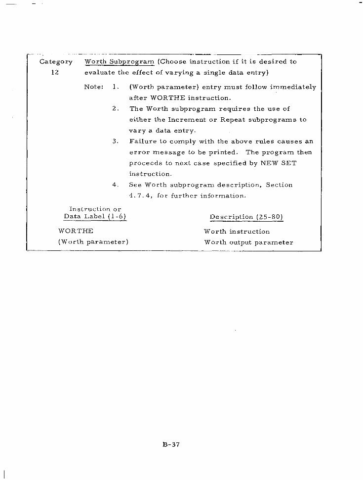
Category Worth Subprogram (Choose instruction if it is desired to
1 2 evaluate the effect of varying a single data entry)
Note: 1.
2.
3 .
4.
Instruct ion or Data Label (1 -6)
(Worth parameter) entry must follow immediately
a f t e r WORTHE instruction.
The Worth subprogram requires the use of
e i ther the Increment o r Repea t subprograms to
v a r y a data entry.
Failure to comply with the above rules causes an
e r r o r m e s s a g e to be printed. The program then
proceeds to next case specified by N E W SET
instruct ion.
See Worth subprogram description, Section
4. 7 . 4 , for fur ther information.
DescriDtion 125-80)
WORTHE Worth instruction
(Wor th pa rame te r ) Worth output parameter "
B-37

Category Nominal System Burdens (Choose desired system burdens
13 data f rom subcategories 13A through 131 as indicated)
Note: 1.
2 .
3.
4.
5.
6 .
Instruction (1 -6) 1 3A
NXANTA
NXANTC
NXANTD
NXANTF
NXANTG
13B
NRANTA
NRANTB NRANTC
.b *"See note 5 above
If no choices are made in a subca tegory pro-
gram automatical ly selects values for system
burdens da ta , un less superseded by a Category
15 (Systems Burden Data) statement.
If a choice is made i n a subca tegory , i t super -
sedes automatic select ion unless superseded
by Category 15 statement.
If more than one choice is made per subca te-
gory p rogram se lec ts first choice.
Entries with dagger ($) a r e t r a n s m i s s i o n r a n g e
dependent and must be supplied by e i ther Cate-
gory 13 or 15 statements when RANGTH
ins t ruc t ion i s se lec ted .
Ent r ies wi th as te r i sk (::) a r e t r a n s m i s s i o n
wavelength dependent and must be supplied by
either Category 13 or 15 statements when
LAMaTH instruct ion is selected.
Failure to comply with above rules causes an
e r r o r m e s s a g e to be printed. The program then
proceeds to next case specified by NEWSET
(see Category 20) instruct ion.
Description (25 -80)
"*Transmitter Antenna Burdens (Choose only one) J-
h = 0. 51 micron, spacecraf t
h = 0. 84 micron, spacecraf t
X = 10.6 microns , spacecraf t
h = 13 cm, d iameter burdens , spacecraf t
A = 13 cm, gain burdens, spacecraf t
::Receiver Antenna Burdens (Choose only one)
A = 0. 51 micron, opt ical d i rect detect ion, ear th
h = 0. 51 micron, opt ical heterodyne, ear th X = 0 . 84 micron, opt ical d i rect detect ion, ear th
B-38

NRANTD
NRANTE
NRANTF
NRANTG
13C
NXACTA
NXACTB
NXACTC
13D
NRACTA
NRACTB
NRACTC
13E
N M ~ D E A
N M ~ D E B
N M ~ D E C
N M ~ D E D
N M ~ D E E
N M ~ D E F
N M ~ D E C
N M ~ D E H
N M ~ D E I
N M ~ D E J
13F
N D M ~ D A
N D M ~ D B
N D M ~ D C
N D M ~ D E
N D M ~ D F
N D M ~ D G .Ir ‘See note 5 above.
X = 10.6 microns, opt ical d i rect detect ion, ear th
X = 10 .6 microns, opt ical heterodyne, ear th
X = 13 cm, d iameter burdens , ear th
X = 13 cm, gain burdens, ear th
Transmit ter Acquis i t ion and Track Burdens (Choose only one)
Optical frequencies, spacecraft
Radio frequencies , spacecraf t , d iameter burdens
Radio frequencies, spacecraft , gain burdens
Receiver Acquisit ion and Track Burdens (Choose only one)
Optical frequencies, earth
Radio frequencies, earth, diameter burdens
Radio frequencies, earth, gain burdens .* “’Modulation Equipment Burdens (Choose only one)
X = 0. 51 micron, CW lase r , spacec ra f t
X = 0.84 micron, CW lase r , spacec ra f t
X = 0.84 micron , pu lsed laser , spacecraf t
X = 10.6 microns , CW lase r , spacec ra f t
X = 13 cm, spacecraf t
X = 0. 51 micron , CW l a s e r , e a r t h
X = 0 . 84 micron, CW l a s e r , e a r t h
X = 0 . 84 micron, pulsed laser , ear th
X = 10. 6 m i c r o n s , CW laser , ea r th
X = 13 cm, ear th
::‘Demodulation Equipment Burdens (Choose only one)
Optical d i rect detect ion, ear th
Optical heterodyne detection, earth
Optical homodyne detection, earth
13 cm radio homodyne detection, earth
Optical direct detection, spacecraft
Optical heterodyne detection, spacecraft
B- 39

N D M ~ D H
NDMQ~DI
NDMQID J
13G
NXMTRA
NXMTRB
NXMTRE
NXMTRF
NXMTRG
NXMTRH
13H
NXP WSA
NXPWSB
NXPWSC
NXPWSD
NXP WSE
NXPWSF
NXPWSG
131
NRPWSA
NRPWSB
NRPWSC
N R P WSD
NRPWSE
NRPWSF
NRPWSG
Optical heterodyne detection, spacecraft
13 cm radio direct detect ion, spacecraf t
13 cm radio homodyne detect ion, spacecraf t * -.Transmitter Burdens (Choose only one)
x = 0. 51 micron, spacecraf t
X = 0. 51 micron , ear th
X = 10.6 microns , spacecraf t
X = 1 0 . 6 m i c r o n s , e a r t h
X = 13 cm, spacecraf t
X = 13 cm, ea r th
$Transmitter System Power Supply Burdens (Choose only one)
RTG, spacecraft
Reactor , spacecraf t
Solar ce l l , Mars , spacecraf t
Genera tor , ea r th
Solar cel l , sa te l l i te , spacecraf t
Solar cell , Venus, spacecraft
Solar cel l , Mercury, spacecraf t
*Receiver System Power Supply Burdens (Choose
only one)
RTG, spacecraft
Reactor , spacecraf t
Solar ce l l , Mars , spacecraf t
Genera tor , ea r th
Solar cell, satel l i te , spacecraf t
Solar cell , Venus, spacecraft
Solar cel l , Mercury, spacecraf t
.Ir
~ .~ ~ ; ~ _ i
"-See note 5 above. 'See note 4 above.
. . " - . ..
B-40

Category System Physical . . Data (Choose desired system physical
14 data- such as s ignal- to-noise ra t io a tmospheric t rans- missivi ty ,
Note: 1.
2 .
3.
4.
5 .
receiver temperature , e tc . as indicated.)
If no choice of an en t ry is made , p rogram au to-
mat ical ly selects a value.
If a choice of an en t ry i s made , it supersedes
automatic selection.
Entries with dagger ( $ ) a re t r ansmiss ion r ange
dependent and must be supplied when RANOTH
instruct ion is selected.
Ent r ies wi th as te r i sk (:::) a re t r ansmiss ion wave -
length dependent and must be supplied when
LAMaTH instruct ion is se lected.
Failure to comply with above rules causes an
e r r o r m e s s a g e to be printed. The program
then proceeds to next case specified by
NEWSET (see Category 20) instruct ion.
Data Label (1 -6)
f RANG * LMDA :k TAUT ':< TAUR >:< TAUA * R H ~ T
* RHOR * TEMP
** ETAA RLLL
** LMDI ** QBEE
PERR SNRR
Data Value (9 -22)
Y Y . . . Y
Y Y . . . Y
Y Y . . . Y
Y Y . . . Y
YY. . . Y
Y Y . . . Y
Y Y . . . Y
Y Y . . . Y
Y Y . . . Y
YY. . . Y
Y Y . . . Y
YY. . . Y
Y Y . . . Y
Y Y . . . Y
Description (25-80)
Transmission range Transmission wavelength Transmitter system transmissivity Receiver system transmissivity
Atmospheric transmissivity Transmitter antenna efficiency Receiver antenna efficiency Receiver equivalent temperature Detector quantum efficiency Receiver output load resistance Optical filter bandwidth Background radiation photon spectral radiance Required probability of detection e r ro r Required signal-to-noise power ratio
**Not Required for Radio Frequency .. . "" -. . ~~~
%See note 4 above. $See note 3 above.
B-4 1

111111
Category System Burdens Data (Choose desired system burdens
15 data as indicated. See Section 4.2 for definition of s y s -
tem burdens da ta . )
Note: 1.
2 .
3 .
4.
5.
If no choice of an en t ry i n a subcategory is
made, program automatical ly selects a value
unless superseded. by a Category 13 s ta tement .
If a choice of an en t ry i n a subcategory is made
it supersedes values selected by Category 13
s ta tement and automatic select ion.
Entries with dagger ( $ ) a r e t r a n s m i s s i o n r a n g e
dependent and must be supplied by e i ther
Category 13 or Category 15 statements when
RANOTH ins t ruc t ion i s se lec ted .
Ent r ies wi th as te r i sk (:::) a r e t r a n s m i s s i o n
wavelength dependent and must be supplied by
ei ther Category 13 or Category 15 s ta tements
when LAMOTH instruction is selected.
Failure to comply with above rules causes an
e r ro r message t o be p r in t ed . The p rog ram
then proceeds to next case specified by
NETSET (see Category 20) instruction.
Label (1-6) Value (9 -22) Description (25-80)
15A $Transmit ter Antenna Burdens
CDT = KTHT::'(DT):k*MT f CKT
HTHT:!(GT)::::::MT f CKT
KTHT HTHT KD T HDT CKT WKT MT NT
Y Y . . . Y Y Y . . . Y Y Y . , . Y YY.. . Y Y Y . . . Y Y Y . . . Y Y Y i . . Y Y Y . . . Y
Note equations above and Section ' 3.0, Symbols
*See note 4 above. B-42

KTHR HTHR KDR HDR CKR WKR MR NR
15B *Receiver Antenna Burdens
CDR = KTHR:k(DR)*<:MR + CKR = HTHR*(GR):k:kMR + CKR
Y Y . . . Y Y Y . . . Y Y Y . . . Y Y Y . . , Y Y Y . . . Y Y Y . . . Y Y Y . . , Y Y Y . . . Y
Note equations above and Section 3 . 0, Symbols
15C Transmitter Acquisit ion and Track Burdens
CQT = KAT:::(DT/LMDA)<:*QT + CAT = WT:::(GT:::%. 5 / ( 3 . 1416*sQRTF(RHOT)))*:::QT + CAT
WQT = KWAT:X(WDT) + WBT
P Q T = KPQT:::(WQT)
KAT Y Y . . . Y
KWAT Y Y . . . Y
KPQT Y Y . . . Y
C A. T Y Y . . . Y
WBT Y Y . . . Y
QT Y Y . , . Y
Note equations above and Section 3 . 0, Symbols
15D Receiver Acquisit ion and Track Burdens
CQR = KAR:k(DR/LMDA)::x:QR t CAR
= KAR<:(1. /GR)<c:::QR + CAR
= KAR*(GR'k*. 5 / ( 3 . 1416%3QRTF(RHOR)))+*QR t CAR
WQR = KWAR:::(WDR) t WBR
PQR = KPQR*(WQR)
-1-
'See note 4 above.
B-43
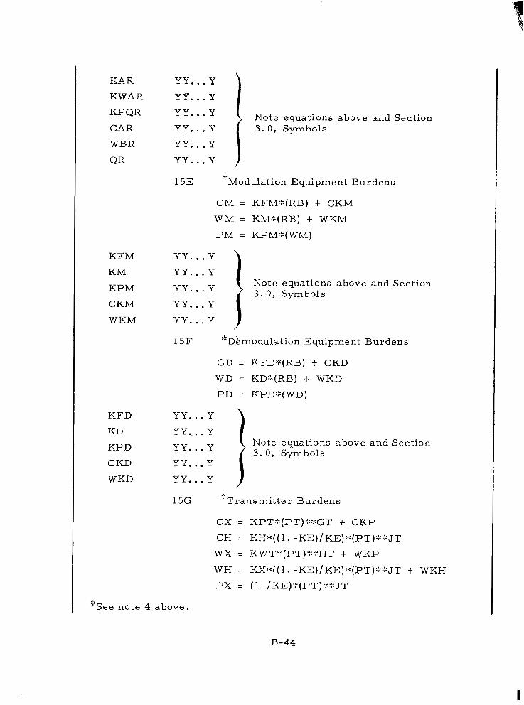
KAR
KWAR
KPQR
CAR
WBR
QR
KFM
KM
KPM
CKM
WKM
KFD
KD
KPD
C KD
WKD
YY. . . Y
YY. . . Y
Y Y . . . Y
Y Y . . . Y
Y Y . . . Y
Y Y . . . Y
I
Note equations above and Section 3 . 0, Symbols
15E ‘Modulation Equipment Burdens 4-
CM = KFM:::(RB) t CKM
WM = KM:::(RB) t WKM
P M = KPM:k(WM)
Y Y . . . Y
Y Y . . . Y
Y Y . . . Y
Y Y . . . Y
YY ... Y
Note equations above and Section ’ 3. 0, Symbols
1 5 F “’DLmodulation Equipment Burdens -8,
CD = KFD’::(RB) t CKD
WD = KD:::(RB) t WKD
P D = KPD:Z(WD)
Y Y . . . Y
Y Y ... . Y
Y Y . . . Y
Y Y . . . Y
Y Y . . . Y i Note equations above and Section 3. 0 , Symbols
.b “’See note 4 above
B-44

K P T
KWT
KH
KX
KE
CKP
CKH
WKP
WKH
G T
HT
J T
KS T
KWST
CKE
WKE
KSR
KWSF.
CKF
WKF
Y Y . . . Y
Y Y . . . Y
Y Y . . . Y
Y Y . . . Y
Y Y . . . Y Y Y . , , Y
Y Y . . . Y
Y Y . . . Y
Y Y . . . Y
YY. . . Y
Y Y . . . Y
Y Y . . . Y
Note equations above and Section 3 . 0 , Symbols
15H *Transmit ter System Power Supply Burdens
CST = KST:::(PQT t P M + P X ) t CKE
WST = KWST':'(PQT t P M t P X ) t WKE
Y Y . . . Y
Y Y . . . Y Note equations above and Section
Y Y . . . Y 3 . 0, Symbols
Y Y . . . Y
151 Receiver System Power Supply Burdens .1< -6-
.CSR = KSR::(PQR t PD) t CKF
WSR = KWSR:::(PQR t P D ) t W K F
Y Y . . . Y ) Y Y . . , Y
Y Y . . . Y
Y Y . . . Y
Note equations above and Section 3 . 0, Symbols
+ See note 3 above.
See note 4 above. .* 1.
B-45

Category System Parameter Constraints Data (Choose system
16 parameter cons t ra in ts da ta as indicated. See Section 4 . 2
for definition of sys t em pa rame te r cons t r a in t s da t a . )
Data Label (1 -6)
DTM
GTM
DRM
GRM
P T M
TRM
DTB
Note: 1.
2 .
3 .
4.
Data
Choose DTM, DTB, and DTL for t ransmi tkr
antenna diameter optimization and GTM,
GTB, and .GTL for transmitter antenna gain
optimization.
Choose DRM, DRB, and DRL for receiver
antenna diameter opt imizat ion and GRM,
GRB, and GRL for receiver antenna gain
optimization.
Choose the maximum and minimum
stop values for the non-f ixed system
p a r a m e t e r s when LAMOTH is chosen.
Fixed system parameters require no
stop values.
Maximum stop value of receiver f ie ld
of view must be smaller than mini-
mum value, TRB TRL. For all
o the r pa rame te r s max imum s top
value must be la rger than min imum
value, XXB>XXL.
Value (9 -22)
Y Y . . . Y
Y Y . . . Y
Y Y . . . Y
Y Y . . . Y
Y Y . . * Y
Y Y . . . Y
Y Y . . . Y
Descript ion (25-80)
Fixed value of t ransmit ter antenna
d i ame te r
Fixed value of transmitter antenna gain
Fixed value of rece iver an tenna d iameter
Fixed value of receiver antenna gain
Fixed value of t ransmi t te r power
Fixed value of receiver f ield of view
Maximum stop value of t r ansmi t t e r
antenna diameter
B-46

Data Label (1 -6)
GTB
DRB
GRB
P T B
TRB
DTL
GTL
DRL
GRL
P T L
TRL
Date Value (9-22)
YY. . . Y
YY. . . Y
YY.. . Y
YY. . . Y
Y Y . . . Y
Y Y . . . Y
Y Y . . . Y
Y Y . . , Y
Y Y . . . Y
Y Y . . . Y
Y Y . . . Y
Description (25-80)
Maximum stop value of t r ansmi t t e r
antenna gain
Maximum stop value of receiver antenna
d iameter
Maximum stop value of rece iver an tenna
gain
Maximum stop value of t r ansmi t t e r
power
Maximum stop value of receiver f ield
of view
Minimum stop value of t r ansmi t t e r
antenna diameter
Minimum stop value of t r ansmi t t e r
antenna gain
Minimum value of receiver antenna
d iameter
Minimum stop value of receiver antenna
gain
Minimum stop value of t ransmit ter power
Minimum stop value of receiver f ield of
view
B-47
IL
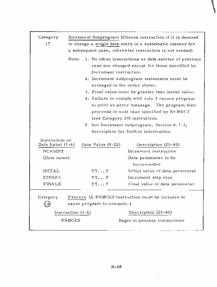
Category Increment Subprogram (Choose instruct ion i f it is des i red
17 to change a s ingle data entry in a systematic manner for
a subsequent case, otherwise instruction is not needed)
Note: 1. No o ther ins t ruc t ions o r da ta en t r ies of previous
case are changed except for those specif ied by
Increment instruction.
2 . Increment subprogram s ta tements must be
arranged in the order shown.
3 . Final value must be greater than init ial value.
4. Failure to comply with rule 3 causes p rog ram
to p r in t an e r ro r message . The p rog ram then
proceeds to next case specified by NEWSET
(see Category 20) instruction.
5. See Increment subprogram, Section 4 . 7 . 2 ,
description for further information.
Ins t ruc t ion or Data Label ( 1 -6) Data Value (9-22) Description (25-80)
NCRMNT Increment instruction
(Data name) Data parameter to be
incremented
INITAL
STPSZE
FINALE
Y Y . . . Y Initial value of da ta parameter
Y Y . . . Y Increment s tep s ize
Y Y . , . Y Final value of da ta parameter
I I
Category Process (A PRaCES instruct ion must be included to
@ cause program to compute. )
Instruction (1 -6)
P R ~ C E S
Description (25-80)
Begin to process instructions
B-48

Category Repeat Subprogram (Choose instruction - i f i t is des i red
19 to change a few ins t ruc t ions o r - data en t r ies for a subse-
quent case otherwise the instruction is not needed)
Note: 1.
2 .
Instruction (1 -6)
REPEAT
xxxxxx xxxxxx
xxxxxx P R ~ C E S
REPEAT
xxxxxx
xxxxxx P R ~ C E S
REPEAT
REPEAT
xxxxxx
xxxxxx P R ~ C E S
. _.I - : . . " . . . - _. .
Only those ins t ruc t ions o r da ta en t r ies of
previous case specif ied by the Repeat
instruct ion are changed.
See Repeat subprogram description, Section
4. 7 . 3 , for fur ther information.
Description (25-80)
f i rs t repeat inst ruct ion
new instruct ions and data for f i rs t repeat instruction
second repeat instruction
new instructions and data for second repeat instruction
third repeat inst ruct ion
las t repeat inst ruct ion
new instruct ions and data for las t repeat inst ruct ion
"_ " "
B-49
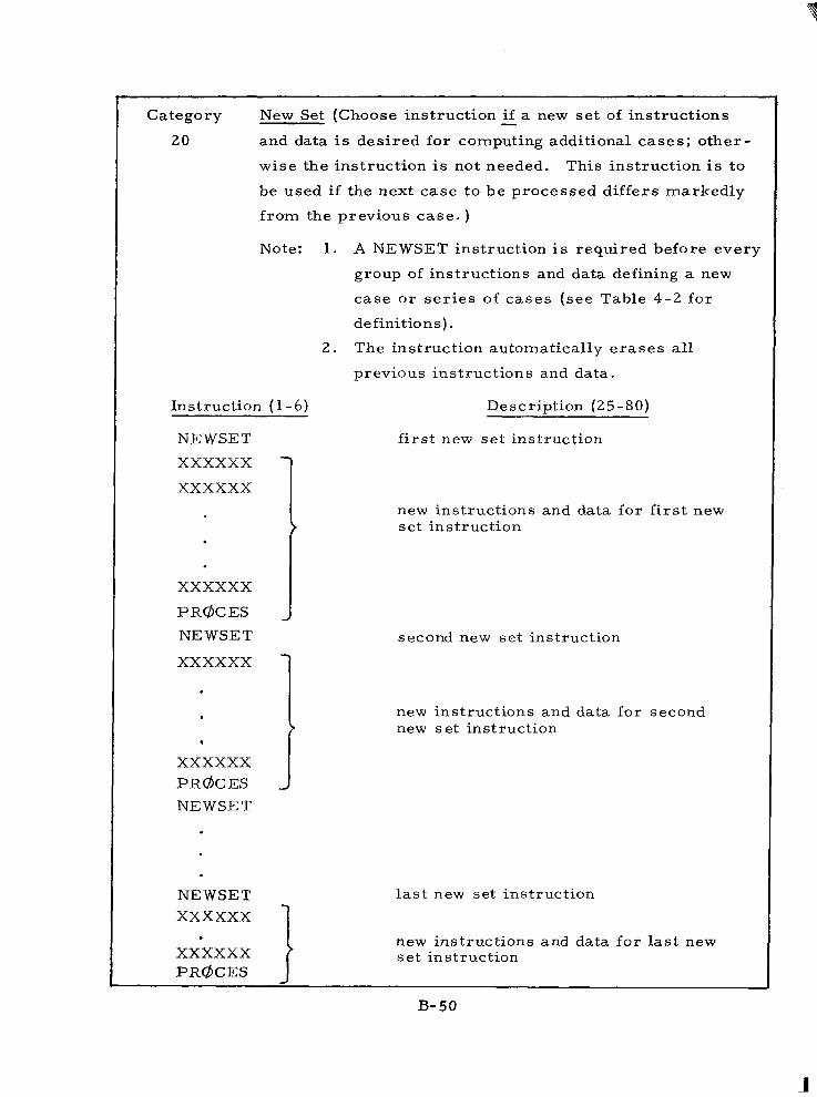
Category New Set (Choose instruction if a new s e t of instruct ions - 20 and data is desired for computing addi t ional cases; o ther-
wise the instruct ion is not needed. This instruction i s to
be used if the next case to be processed differs markedly
f rom the p rev ious case . )
Note: 1. A NEWSET instruction i s required before every
group of instructions and data defining a new
c a s e o r s e r i e s of cases ( see Table 4 - 2 for
definit ions).
2 . The instruct ion automatical ly erases all
previous instruct ions and data .
Instruction (1 - 6 )
NEWSET
xxxxxx xxxxxx
xxxxxx P R ~ C E S NEWSET
xxxxxx
t
xxxxxx P R ~ C E S NEWSET
NEWSET xxxxxx xxxxxx P R ~ C E S
Description (25-80)
f i r s t new se t ins t ruc t ion
new instruct ions and data fo r first new set inst ruct ion
second new set inst ruct ion
new instruct ions and data for second new set inst ruct ion
l a s t new set inst ruct ion
new instruct ions and data for las t new se t ins t ruc t ion
B- 5 0

- ~~~ ~ - " - -~ ~~
Category End of Run (An ENDRUN instruction must follow all
0 other instruct ions and data entr ies)
Instruction ( 1 -6) Description (25-80)
ENDRUN End of processing run
." . .. . _" . - . . -" ~~ "
B-5 1
I -


Example C
Example C i l lustrates the optimization of a heterodyne detection optical
communication system (HOPS example) using the complete listing of COPTRAN
instructions and data with the Repeat subprogram. The communication system
optimization problem is summarized below.
Jupi te r Spacecraf t Transmi t te r to Ear th Rece iver L ink
10.6 micron t ransmission wavelength
PCM frequency shift keying and optical heterodyne detection receiver
Transmitter system weight optimization
Parameters to be op t imized:
a. Transmi t te r an tenna d iameter
b. Receiver antenna diameter
c . Transmit ter power
F ixed parameters :
a. Receiver f ie ld of view at 1 mill iradian
Pa rame te r s tops :
a. Transmit ter power a t 1 kw
b. Receiver antenna diameter a t 1 m e t e r
c . Transmi t te r an tenna d iameter a t 50 cm and 80 cm
A COPTRAN coding sheet for this example is shown on the next page followed
by the computer tabulation and plots for the example.
B-53

1

. . . . . . . . . . . . . . . . . . . . . . . . . . . . . . . . . . . . . . . . . . . . . . . . . . . . . . . . . . . . . . . . EXAHPLr i HOPS *
. . . . . . . . . . . . . . . . . . . . . . . . . . . . . . . . . . . . . . . . . . . . . . . . . . . . . . . . . . . . . . . .
1

c 0
B-56

0.IOOC 01 0.1008 03 0.soor' 02 O.IUOE'02


2onon.00
15nun.no
0.Y80FO
o .wono
1 . 9 n ~ n o o.ono
5.unono
3.3mno
12nu000.
5000.
nATA
VKT
VKP
CAT
CAI,
WX J T
CKM
CKll
VKF
WKC
*.no
2.000no
uo.ono
s.ono
0.1oono I .onon0
10.00
55.000
NT
Na
e1
OR
CKP HT
2.10000
?.00000
0.30000
n.abaaa
lno,oo..no 1.00000


**e COPTRAN PUOGRAM *** SPXMTR LARCVR RAHJUP BKDWcl LAM106 PCWFM OPTnET XHllOP RUIN~O RBFIN7 LeFRa9 TITLEE PRTDAT PLloPT PT0 DUM Dl0 TRH
0.lUOC u 0.1COE u 0.500E U 0.100t-C
IY 15 I2 12

TRANSMITTED ANTENNA
RbCLIVER ANTENNA
ACOUISITIohl TRANSMITTER
A N D TRLCK SYSTEM
.RECEiVER A C ~ ~ I S I T I O N AND TRACK SYSTEM
THANSMITTEP
MODULATION EQUIPMENT
DEMODULATION EQUIPMENT
THANSNITTER POwtR SUPPLV
RECE I VER PoUtR SUPPLY
BOOSTER 8UROENS
71000.
CKH 1.Y3UOU
1JR00.
KFM o.onu50
kFU 0.0001110U
KST 500.000
KSH 2 5 . ~ 0 0
KSA 16'bO.UOO
KCAH .O.'b6000
KWSH 0.OOOOnOO
KSP I IY+O.~OO
?onon.oo
25noo.no
0.Y8000
o.unono
1.970110 o.ono
s.onooo
~ 3 3 o n o
12n0000.
5000.
UKT
YKR
CAT
CAR
K X JT
CKY
CKO
YKF
UKF
*.no
2.00000
@O+OOQ
s.000
O * ? P Q b q I .ooono
m.no
'J5.00-0,
2.20000.
" i.eoo,o
d.WO..
a.saa0i
0 . 0 Y%:o"-

2i I
I
B- 66

CR-1687 NASA-Langley, 1970 - 7 B- 67