Embed Size (px)
Citation preview
Parametric Lorenz Curves and the Modality of
the Income Density Function
Melanie Krause ∗
Goethe University Frankfurt
DRAFT VERSION 11.11.12
FOR FINAL, REVISED VERSION SEEReview of Income and Wealth 60, 2014, pp.905-929
Abstract
Similar looking Lorenz Curves can imply very different income density functions and
potentially lead to wrong policy implications regarding inequality. This paper derives
a relation between a Lorenz Curve and the modality of its underlying income density:
Given a parametric Lorenz Curve, it is the sign of its third derivative which indicates
whether the density is unimodal or zeromodal (i.e. downward-sloping). Several single-
parameter Lorenz Curves such as the Pareto, Chotikapanich and Rohde forms are
associated with zeromodal densities. The paper contrasts these Lorenz Curves with the
ones derived from the (unimodal) Lognormal density and the Weibull density, which,
remarkably, can be zero- or unimodal depending on the parameter. A performance
comparison of these five Lorenz Curves with Monte Carlo simulations and data from
the UNU-WIDER World Income Inequality Database underlines the relevance of the
theoretical result: Curve-fitting of decile data based on criteria such as mean squared
error might lead to a Lorenz Curve implying an incorrectly-shaped density function. It
is therefore important to take into account the modality when selecting a parametric
Lorenz Curve.
JEL Classification: C13, C16, D31, O57
Keywords: Lorenz Curve, Income Distribution, Modality, Inequality, Goodness of Fit
1 Introduction
In the macroeconomic field of growth and development it is not only of interest to analyze
a country’s total GDP but also how it is distributed across the population. A widely used
concept to express inequality is the Lorenz Curve L(π), developed by Lorenz (1905), which
∗Correspondence address: Goethe University Frankfurt, Faculty of Economics and Business Admin-
istration, Chair for International Macroeconomics & Macroeconometrics, Grueneburgplatz 1, House of
Finance, 60323 Frankfurt am Main, Germany; E-mail address: [email protected];
[email protected]. The author is grateful for comments and suggestions to seminar participants
at Goethe University, the RGSE conference in Duisburg, the IAES conference in Istanbul and the ’Jahresta-
gung des Vereins für Socialpolitik’ in Göttingen.
1
links the cumulative income share L to the cumulative share π of people in the population
earning an income up to this level. When income becomes more equally distributed, the LC
approaches the 45 degree line. An example of different LCs is depicted in Figure (1).
0 0.1 0.2 0.3 0.4 0.5 0.6 0.7 0.8 0.9 10
0.1
0.2
0.3
0.4
0.5
0.6
0.7
0.8
0.9
1
Population share π
Inco
me
shar
e L(
π)
Figure 1: Illustration of Different Lorenz Curves
Given empirical data, the choice of the appropriate functional form for the LC is usually
based on a goodness of fit criterion such as Mean Squared Error. This paper argues, how-
ever, that such a choice might be misleading because very similar looking LCs can imply
very different shapes of the underlying income density f(x). It proposes a way to infer the
modality of an income density from the functional form of the LC so that researchers can
take it into account when choosing among various LC functions.
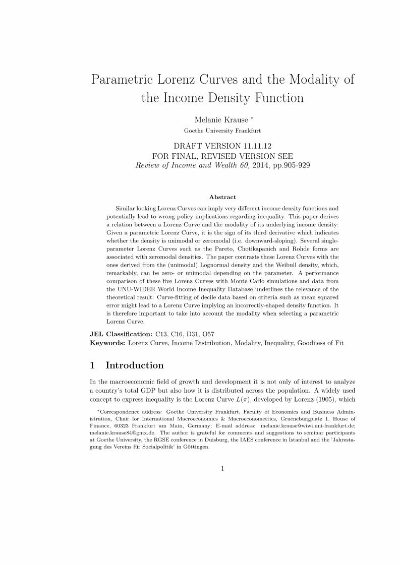
The modality - the number of modes - vitally determines the shape of a density: Figure (2)
shows three density functions of different modality, namely zeromodal (downward-sloping)
f0(x), the normal distribution as an example of a unimodal density f1(x) and a bimodal
normal mixture f2(x).
In this paper I argue that the third derivative of an LC indicates the modality of its under-
lying income density. So it is not necessary to derive the density explicitly (which can be
tedious).
It is generally acknowledged and pointed out e.g. by Dagum (1999) and Kleiber (2008)
that wealth densities tend to be zeromodal, whereas income densities are typically unimodal
(unless a country is very poor and overpopulated). However, several single-parameter LCs
used in empirical income studies belong to zeromodal densities. These are for example the
Pareto LC (see Arnold (1983)) and the LCs proposed by Chotikapanich (1993) and Rohde
(2009). This paper contrasts these LCs with ones associated with unimodal densities, like
the Lognormal density. A particular focus of my analysis lies on the LC associated with the
2
0 0.5 1 1.5 2 2.5 3 3.5 4 4.5 50
0.1
0.2
0.3
0.4
0.5
0.6
0.7
0.8
0.9
1
Variable x
Pro
babi
lity
Den
sity
Fun
ctio
n f
Zeromodal density f0(x)
Unimodal density f1(x)
Bimodal density f2(x)
Figure 2: Density Functions with Different Modalities
Weibull density because, depending on the value of its shape parameter, this density can be
either zeromodal or unimodal.
These five LCs are then used in a Monte Carlo simulation highlighting the relevance of
a density’s modality: Draws are taken from a given density and then aggregated to decile
points, the usually available format in large cross-country data sets. Will the LC best fitting
these decile points in a Mean Squared Error way imply a density with the correct shape?
And, given the answer is no, how can the researcher avoid such a situation in practice, when
the underlying modality is unknown? An application of the five LCs to decile data from the
United Nations University - World Institute for Development Economics Research (2008)
gives further insights.
This paper is structured as follows: In Section 2 the theoretical result on the relation
between the LC and the modality of its density function is derived, while in Section 3 it
is applied to the Pareto, Chotikapanich, Rohde, Lognormal and Weibull LCs. The Monte
Carlo Simulation is carried out in Section 4 and the empirical analysis follows in Section 5.
Section 6 briefly concludes. Some technical derivations and large tables have been relegated
to the Appendix.
2 Relation between the Lorenz Curve and the modality
of its density
Let us start with the formal definition of an LC L(π) by Kakwani and Podder (1973) and
Kakwani and Podder (1976):
3
Definition 1. A function L(π), continuous on [0, 1] and with second derivative L′′(π), is a
Lorenz Curve (LC) if and only if
L(0) = 0, L(1) = 1, L′(0+) ≥ 0, L′′(π) ≥ 0 in (0,1) (1)
A density f(x) with mean µ, cumulative distribution π = F (x) and its inverse function
x = F−1(π) is related to its LC L(π) by the following formula (see Gastwirth (1971) and
Kakwani (1980)):
F−1(π) = L′(π)µ (2)
Hence, starting with a given income density with f(x) and π = F (x), one can obtain the
LC as follows: Find the inverse cumulative distribution function x = F−1(π) and divide it
by µ to obtain the slope L′(π) of the LC. Integrating with respect to π and making sure
that the properties from (1) are fulfilled gives L(π).
The modality of the density function f(x) can be defined formally in terms of sign
changes in its first derivative f ′(x):
Definition 2. The modality of a continuously differentiable density f(x) on [xL, xU ] is the
number of local maxima x̃ ∈ (xL, xU ) where
f ′(x̃) = 0,
f ′(x) > 0 ∀x ∈ X̃N ∧ x < x̃
f ′(x) < 0 ∀x ∈ X̃N ∧ x > x̃,
(3)
with X̃N denoting the neighborhood of the point x̃.
In the following, I will make use of a result by Arnold (1987), who differentiates (2) with
respect to x and summarizes the relation in his theorem:
Theorem 1. If for the Lorenz Curve L(π) the second derivative L′′(π) exists and is positive
in an interval (x1, x2), then F (x) has a finite positive density in the interval (xL, xU ) =(µL′(F (x+
1 )), µL′(F (x−
2 )))
which is given by
f(x) =1
µL′′ (F (x))(4)
Proof. See Arnold (1987).
A key contribution of this paper is the following theorem on the relation between the
LC and the modality of its density:
Theorem 2. If the LC L(π) has a third derivative L′′′(π) and the cumulative distribution
F (x) has a finite positive and differentiable density f(x) in the interval (xL, xU ), it holds:
• If and only if L′′′(π) > 0 ∀π ∈ (0, 1), then f ′(x) < 0 ∀x ∈ (xL, xU ). This means that
f(x) is zeromodal and downward-sloping.
4
• If and only if L′′′(π) < 0 ∀π ∈ (0, 1), then f ′(x) > 0 ∀x ∈ (xL, xU ). This means that
f(x) is zeromodal and upward-sloping.
• If and only if L′′′(π) = 0 ∀π ∈ (0, 1), then f ′(x) = 0 ∀x ∈ (xL, xU ). This means that
f(x) is constant; the distribution is uniform.
• If and only if L′′′(π) < 0 ∀π < π̃ = F (x̃) and L′′′(π) > 0 ∀π > π̃ = F (x̃), then
f ′(x) > 0 ∀x < x̃ and f ′(x) < 0 ∀x > x̃. This means that f(x) is unimodal with mode
x̃.
• In general: If and only if L′′′(π) has n ≥ 1 sign changes from L′′′(π) < 0 to L′′′(π) > 0
occurring at n points π̃i (with i = 1, ..., n), then f ′(x) shows the corresponding sign
changes from f ′(x) > 0 to f ′(x) < 0 occurring at the n points x̃i (with i = 1, ..., n).
This means that f(x) is n-modal with modes at x̃i (with i = 1, ..., n).
Proof. Differentiating (4) with respect to x, one arrives at
f ′(x) = − f(x)
µ[L′′(F (x))]2L′′′(F (x)). (5)
Note that f(x), µ and [L′′(F (x))]2 are positive, so there is a negative relative between f ′(x)
and L′′′(F (x)). From Definition (2) one can express the modality of a density in terms of
f ′(x), with a sign change in f ′(x) occurring at a mode x̃. The combination of these two
results is the relation between L′′′(F (x)) and the density modality as stated in the theorem,
with a sign change in L′′′(F (x)) corresponding to a mode x̃.
Some of the cases from Theorem (2) are more practically relevant than others: The
second and third case, upward-sloping zeromodal and constant income densities have been
included here for mathematical rigor, but are of limited practical use and will be neglected
henceforth. Because of their empirical importance for income and wealth distributions, the
focus of the remainder of this paper will be on unimodality and (downward-sloping) zero-
modality, although according to Theorem (2), the theoretical result applies to distributions
of a higher modality as well.
So it is the sign of the third derivative of the LC which determines the modality of the
underlying density function. By Definition (1), the first and second derivatives of an LC are
positive. If the third derivative is positive as well, the density is zeromodal, but if its sign
changes n-times from negative to positive, the density is n-modal. This means that given
any parametric LC, one can infer the shape of the underlying density just from looking at its
third derivative, without explicitly deriving the density. In the following, I will discuss the
implications of this insight for LC fitting in practice. Because of the empirical importance
for income and wealth distributions, the focus will be on zeromodality and unimodality,
although as shown in (2), the theoretical result applies to distributions of a higher modality
as well.
5
3 The density modality of some parametric LCs
3.1 The Pareto, Chotikapanich and Rohde LCs
A number of parametric forms have been proposed to fit empirical LCs and they can have
one or more parameter; for an overview see Ryu and Slottje (1999) and Sarabia (2008).1
While multi-parameter LCs, such as the forms suggested by McDonald (1984), Dagum
(1977), Villasenor and Arnold (1989) and Basmann et al. (2002), tend to achieve a better
fit than their single-parameter counterparts, they entail an increased complexity in estimat-
ing the parameters, see e.g. Ryu and Slottje (1999). Single-parameter curves are known for
their simplicity, ease of parameter interpretation, and crucially, feasibility in the presence
of scarce data. In broad cross-country datasets often only decile data points are available,
so this paper will concentrate on single-parameter LCs.
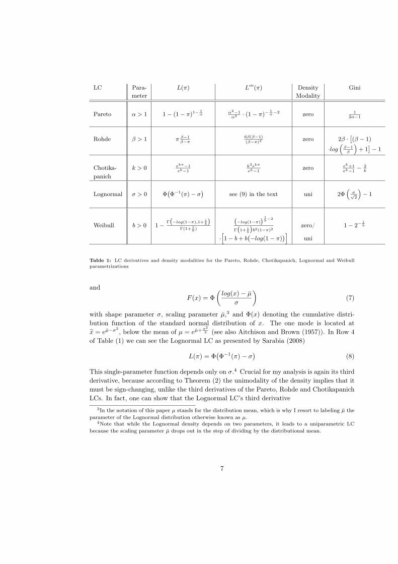
As examples, let us consider the well-known Pareto LC (see Arnold (1983)) and the forms
proposed by Chotikapanich (1993) and more recently by Rohde (2009). Their parametric
forms L(π) are given in the first three rows of Table (1). There one can also find their third
derivatives L′′′(π), which, intriguingly, are all positive on the whole domain. According
to Theorem (2), this means that the income density functions associated with these three
LCs are zeromodal.2 One should bear in mind that these LC parametrizations are used in
empirical studies with income data - which is often unimodal. One could argue that, given
the positivity restriction of L′(π) and L′′(π), it is more obvious to find single-parameter forms
whose third derivative is positive as well rather than sign-changing. Indeed, expressions for
the latter parametric LCs tend to be algebraically more involved, as we will see in the
following, when we consider the Lognormal and Weibull forms.
3.2 The Lognormal LC
A widely-used example of a unimodal income distribution is the Lognormal, whose density
and cumulative distribution function are given by:
f(x) =1
x√2πσ2
e−(log(x)−µ̄)2
2σ2 (6)
1For the merits and drawbacks of parametric LCs compared to their non-/semiparametric counterparts,
see Ryu and Slottje (1999). Research is advancing in both strands, consider e.g. Sarabia (2008) and Rohde
(2009) on parametric LCs and Hasegawa and Kozumi (2003) and Cowell and Victoria-Feser (2007) on non-
/semiparametric LCs. One should be aware that the structural assumptions underlying parametric LCs
might be a limitation, however, they offer the only feasible estimation approach in the presence of decile
data.2Because the density functions of these parametric LCs are known, one could also look at them directly
to check their zeromodality. For instance, Rohde (2009) has derived the income density of his LC as
f(x) = 12
√β(β−1)µ
x3 ∀x ∈
[(β−1)µ
β; βµβ−1
]. However, Theorem (2) allows to infer its zeromodality without
having to derive the functional form of the density explicitly.
6
LC Para- L(π) L′′′(π) Density Gini
meter Modality
Pareto α > 1 1− (1− π)1−1α
α2−1α3 · (1− π)−
1α−2 zero 1
2α−1
Rohde β > 1 π β−1β−π
6β(β−1)
(β−π)4zero 2β ·
[
(β − 1)
·log(
β−1β
)
+ 1]
− 1
Chotika- k > 0 ekπ−1ek−1
k3ekπ
ek−1zero ek+1
ek−1−
2k
panich
Lognormal σ > 0 Φ(
Φ−1(π)− σ)
see (9) in the text uni 2Φ(
σ√2
)
− 1
Weibull b > 0 1−Γ(
−log(1−π),1+ 1b
)
Γ(1+ 1b)
(
−log(1−π)) 1
b−2
Γ(
1+ 1b
)
b2(1−π)2zero/ 1− 2−
1b
·
[
1− b+ b(
−log(1− π))
]
uni
Table 1: LC derivatives and density modalities for the Pareto, Rohde, Chotikapanich, Lognormal and Weibull
parametrizations
and
F (x) = Φ
(log(x)− µ̄
σ
)(7)
with shape parameter σ, scaling parameter µ̄,3 and Φ(x) denoting the cumulative distri-
bution function of the standard normal distribution of x. The one mode is located at
x̃ = eµ̄−σ2
, below the mean of µ = eµ̄+σ2
2 (see also Aitchison and Brown (1957)). In Row 4
of Table (1) we can see the Lognormal LC as presented by Sarabia (2008)
L(π) = Φ(Φ−1(π)− σ
)(8)
This single-parameter function depends only on σ.4 Crucial for my analysis is again its third
derivative, because according to Theorem (2) the unimodality of the density implies that it
must be sign-changing, unlike the third derivatives of the Pareto, Rohde and Chotikapanich
LCs. In fact, one can show that the Lognormal LC’s third derivative
3In the notation of this paper µ stands for the distribution mean, which is why I resort to labeling µ̄ the
parameter of the Lognormal distribution otherwise known as µ.4Note that while the Lognormal density depends on two parameters, it leads to a uniparametric LC
because the scaling parameter µ̄ drops out in the step of dividing by the distributional mean.
7
L′′′(π) =φ′′(Φ−1(π)− σ) · φ(Φ−1(π))− φ(Φ−1(π)− σ) · φ′′(Φ−1(π))
[φ(Φ−1(π))]4(9)
−3[φ′(Φ−1(π)− σ) · φ′(Φ−1(π))− φ(Φ−1(π)−σ)
φ(Φ−1(π)) · (φ′)2(Φ−1(π))]
[φ(Φ−1(π))]4
is indeed sign-changing from negative to positive, with the change occurring at π̃ =
F (x̃) = Φ(−σ).
3.3 The Weibull LC
As this paper focuses on the relation between the LC and the modality of the underlying
income density, one functional form deserves particular attention: The Weibull density and
distribution function given by
f(x) =b
a
(xa
)b−1
e−(xa )
b
(10)
F (x) = 1− e−(xa )
b
(11)
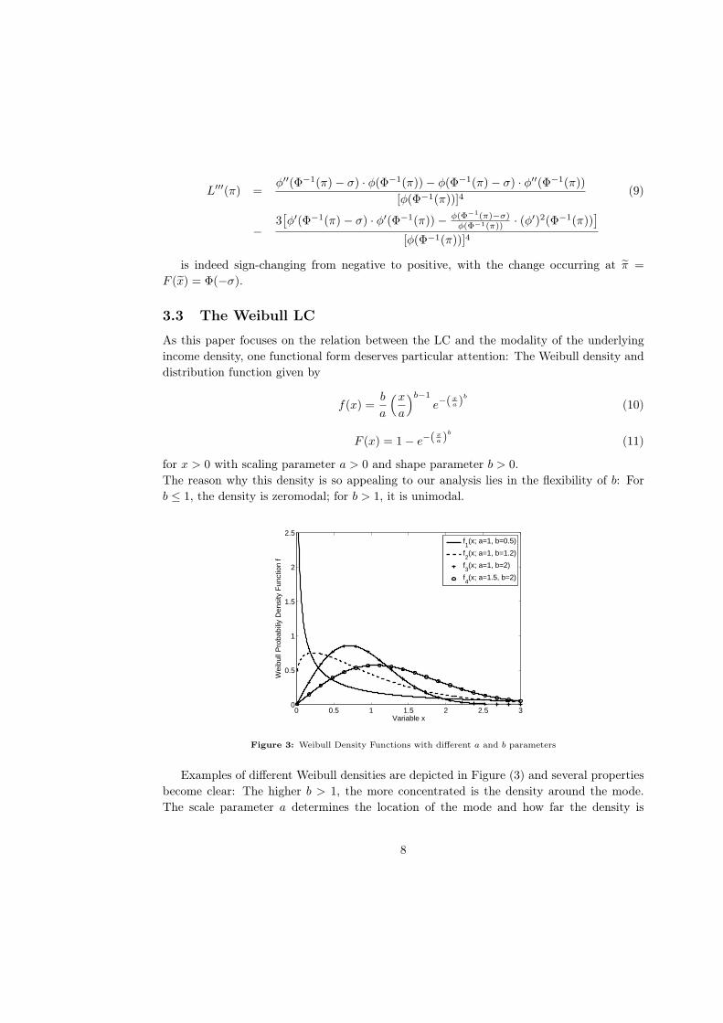
for x > 0 with scaling parameter a > 0 and shape parameter b > 0.
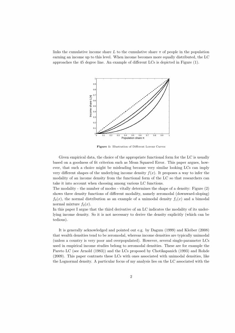
The reason why this density is so appealing to our analysis lies in the flexibility of b: For
b ≤ 1, the density is zeromodal; for b > 1, it is unimodal.
0 0.5 1 1.5 2 2.5 30
0.5
1
1.5
2
2.5
Variable x
Wei
bull
Pro
babi
liy D
ensi
ty F
unct
ion
f
f1(x; a=1, b=0.5)
f2(x; a=1, b=1.2)
f3(x; a=1, b=2)
f4(x; a=1.5, b=2)
Figure 3: Weibull Density Functions with different a and b parameters
Examples of different Weibull densities are depicted in Figure (3) and several properties
become clear: The higher b > 1, the more concentrated is the density around the mode.
The scale parameter a determines the location of the mode and how far the density is
8
spread out, but the shape is entirely captured by b. The Weibull density allows for positive
skewness; in particular, small values of b > 1 lead to unimodal and strongly positively skewed
densities. These properties make the Weibull density suitable for modeling (unimodal)
income densities, while also representing zeromodal densities with b ≤ 1. The Weibull
distribution is a special case of the Generalized Beta distribution. In this context, its
ability to model income densities has been analyzed by McDonald (1984) and McDonald
and Ransom (2008).
However, the single-parameter LC pertaining to the Weibull density does not seem to
have appeared in the literature yet, so I derive its functional form here.
Theorem 3. The LC associated with a Weibull distributed variable x with π = F (x) given
in (11) has the single-parameter LC
L(π) = 1− Γ(−log(1− π), 1 + 1
b
)
Γ(1 + 1b)
(12)
where Γ(α) =∫∞
0tα−1e−tdt is the Gamma function and Γ(x, α) =
∫∞
xtα−1e−tdt is the
upper incomplete Gamma function.
Proof. See Appendix A.
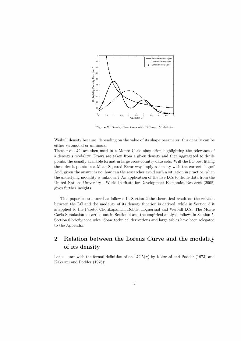
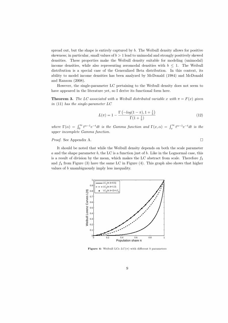
It should be noted that while the Weibull density depends on both the scale parameter
a and the shape parameter b, the LC is a function just of b. Like in the Lognormal case, this
is a result of division by the mean, which makes the LC abstract from scale. Therefore f3
and f4 from Figure (3) have the same LC in Figure (4). This graph also shows that higher
values of b unambiguously imply less inequality.
0 0.2 0.4 0.6 0.8 10
0.1
0.2
0.3
0.4
0.5
0.6
0.7
0.8
0.9
1
Population share π
Wei
bull
Lore
nz C
urve
s L(
π)
LC
1(π; b=0.5)
LC2(π; b=1.2)
LC3(π; b=2)=LC
4
Figure 4: Weibull LCs LC(π) with different b parameters
9
Row 5 of Table (1) presents the Weibull LC and its third derivative, which I derive as
L′′′(π) =
(−log(1− π)
) 1b−2
Γ(1 + 1
b
)b2(1− π)2
[1− b+ b
(−log(1− π)
)](13)
From Theorem (2) it directly follows that L′′′(π) is positive for b ≤ 1, implying a zero-
modal density, and sign-changing for b > 1, implying a unimodal density. In the latter
case, L′′′(π) = 0 occurs at the point π̃ referring to the mode x̃ = a(1− 1
b
) 1b of the Weibull
density. For an alternative proof of these properties, see Appendix B.
4 Monte Carlo Simulation
Section 3 has illustrated Theorem (2) on the relation between an LC’s third derivative and
the modality of its income density, using as examples of the Pareto, Rohde, Chotikapanich,
Lognormal and Weibull LCs. Let us now turn to the practical importance of this theoretical
insight: When a researcher fits decile data points to different LCs and chooses the one with
the best fit, what will the density of this LC look like?
For the purpose of deciding which of the five parametric LCs has the best fit, this paper
uses two complementary criteria: the Mean Squared Error (MSE) and the Gini difference.
While the MSE indicates how well the parametric LC fits the given (decile) data points, the
Gini difference (see Chotikapanich (1993)) exploits the relation between the Gini coefficient
and the LC:
Gini = 1− 2
∫ 1
0
L(π)dπ (14)
Having estimated the parametric LC to fit the data, one can calculate the Gini implied
by the LC according to this formula. The Gini difference is then obtained as the absolute
difference between the implied Gini and the actual one. In contrast to MSE, the Gini dif-
ference captures the overall fit of the shape of the LC rather than only the fit at the decile
data points.
The last column of Table (1) in Section 3 shows the Gini coefficients implied by the five
parametric LCs.5 One should note the sign of the relation between the functional parameter
and the Gini: A higher Pareto α, Rohde β and Weibull b are associated with less inequal-
ity, while a higher Chotikapanich k and Lognormal σ imply a more inegalitarian distribution.
The MC Simulation is carried out as follows:
1. Take 10,000 draws from a fixed underlying income density with zeromodal or unimodal
shape and mean 1.
5These formulas can be found, respectively, in Arnold (1983) (for the Pareto LC), Rohde (2009), Chotika-
panich (1993) (I use a simplified expression of her formula) and McDonald (1984) (with the Weibull and
Lognormal distributions as special cases of the Generalized Beta).
10
2. The drawn income data is aggregated to decile data points (which is the usually
available data format in large cross-country income inequality datasets).
3. For each of the five parametric forms, calculate the parameter which best fits the
decile data points by minimizing the MSE.6 This procedure is carried out using the
fminunc-routine in MatLab.
4. The MSE and the Gini difference are calculated for each of the five parametric forms
and stored.
5. Steps 1 to 4 are repeated 10,000 times.
6. Look which of the five parametric forms has the lowest MSE and/or Gini difference
overall: Does the density implied by this LC have the correct shape, that is, does it
look similar to the actual one?
I put the answer upfront - it is clearly no. It is an important conclusion of this paper
that the researcher cannot rely upon decile point MSE or Gini difference to pick an LC
whose density has the correct shape. Instead he/she should limit their choice upfront to the
LCs with the correct density modality.
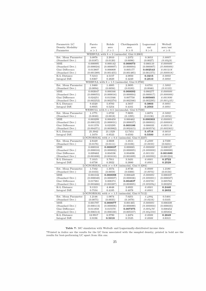
Table (7) in Appendix C displays the results when the underlying density is Lognormal
or Weibull, for varying inequality levels.7 Of course, fitting an LC of this given form always
leads to the lowest MSE and Gini difference. But the focus lies on which of the other LC
forms does best, highlighted in bold. For instance, for an underlying egalitarian Weibull
density (with b=3), a fitted Chotikapanich LC leads to the lowest MSE at the decile data
points. If, based on this criterion, the researcher chose the Chotikapanich LC, the implied
density would be zeromodal and very different from the true Weibull density. Figures (5)
and (6) show the LCs and densities for this case. The very similar looking LCs give rise to
considerably varying income densities. A researcher aware of the unimodality of his data
should rather decide on the Lognormal LC, which, despite its slightly higher MSE at the
given decile points, captures the unimodal shape of the Weibull income density. A diverging
shape might lead to incorrect conclusions about the distribution of income, because the
downward-sloping Chotikapanich density misses out on the dominance of the middle class
and implies a larger number of comparatively poor earners. As Table (7) shows, the Gini
difference as goodness of fit criterion would (appropriately) point towards the Lognormal
LC in the above setting. But in other MC simulations, this paper finds no evidence for a
general superiority of the Gini difference over MSE in selecting an LC whose density has
the correct shape.
6When using the Mean Absolute Error rather than the Mean Squared Error for LC fitting at the decile
points, the relative performance of the five parametric forms remains mostly unchanged. Only the Pareto
form tends to obtains a slightly better fit with this criterion, which penalizes large deviations less severely.7When conducting the simulations with other underlying densities other than the five discussed here, the
overall results and implications of modality and the goodness of fit criteria are similar.
11
0 0.2 0.4 0.6 0.8 10
0.1
0.2
0.3
0.4
0.5
0.6
0.7
0.8
0.9
1
Population share π
Inco
me
shar
e L(
π)
Pareto Lorenz Curve (α = 3.0976)Rohde Lorenz Curve (β = 2.2010)Chotikapanich Lorenz Curve (k = 1.2372)Lognormal Lorenz Curve (σ = 0.3653)(True) Weibull Lorenz Curve (b=3)
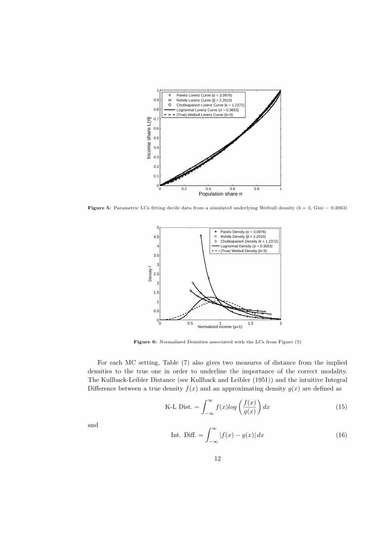
Figure 5: Parametric LCs fitting decile data from a simulated underlying Weibull density (b = 3, Gini = 0.2063)
0 0.5 1 1.5 20
0.5
1
1.5
2
2.5
3
3.5
4
4.5
5
Normalized income (µ=1)
Den
sity
f
Pareto Density (α = 3.0976)Rohde Density (β = 2.2010)Chotikapanich Density (k = 1.2372)Lognormal Density (σ = 0.3653)(True) Weibull Density (b=3)
Figure 6: Normalized Densities associated with the LCs from Figure (5)
For each MC setting, Table (7) also gives two measures of distance from the implied
densities to the true one in order to underline the importance of the correct modality.
The Kullback-Leibler Distance (see Kullback and Leibler (1951)) and the intuitive Integral
Difference between a true density f(x) and an approximating density g(x) are defined as
K-L Dist. =
∫ ∞
−∞
f(x)log
(f(x)
g(x)
)dx (15)
and
Int. Diff. =
∫ ∞
−∞
|f(x)− g(x)| dx (16)
12
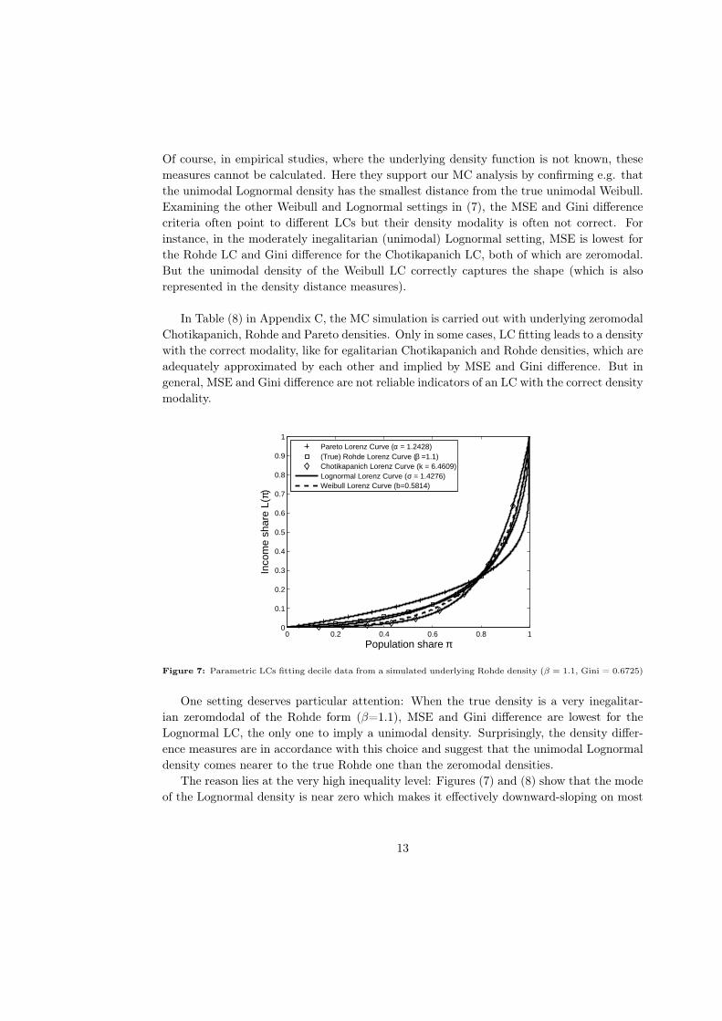
Of course, in empirical studies, where the underlying density function is not known, these
measures cannot be calculated. Here they support our MC analysis by confirming e.g. that
the unimodal Lognormal density has the smallest distance from the true unimodal Weibull.
Examining the other Weibull and Lognormal settings in (7), the MSE and Gini difference
criteria often point to different LCs but their density modality is often not correct. For
instance, in the moderately inegalitarian (unimodal) Lognormal setting, MSE is lowest for
the Rohde LC and Gini difference for the Chotikapanich LC, both of which are zeromodal.
But the unimodal density of the Weibull LC correctly captures the shape (which is also
represented in the density distance measures).
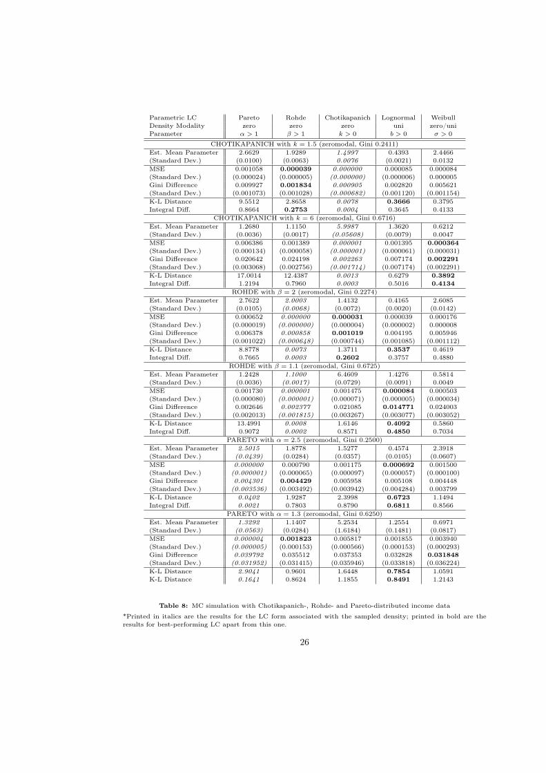
In Table (8) in Appendix C, the MC simulation is carried out with underlying zeromodal
Chotikapanich, Rohde and Pareto densities. Only in some cases, LC fitting leads to a density
with the correct modality, like for egalitarian Chotikapanich and Rohde densities, which are
adequately approximated by each other and implied by MSE and Gini difference. But in
general, MSE and Gini difference are not reliable indicators of an LC with the correct density
modality.
0 0.2 0.4 0.6 0.8 10
0.1
0.2
0.3
0.4
0.5
0.6
0.7
0.8
0.9
1
Population share π
Inco
me
shar
e L(
π)
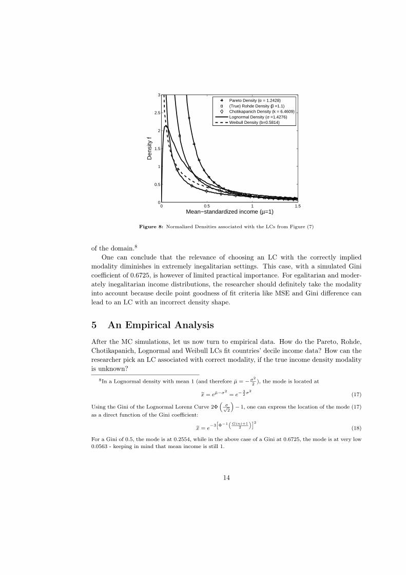
Pareto Lorenz Curve (α = 1.2428)(True) Rohde Lorenz Curve (β =1.1)Chotikapanich Lorenz Curve (k = 6.4609)Lognormal Lorenz Curve (σ = 1.4276)Weibull Lorenz Curve (b=0.5814)
Figure 7: Parametric LCs fitting decile data from a simulated underlying Rohde density (β = 1.1, Gini = 0.6725)
One setting deserves particular attention: When the true density is a very inegalitar-
ian zeromdodal of the Rohde form (β=1.1), MSE and Gini difference are lowest for the
Lognormal LC, the only one to imply a unimodal density. Surprisingly, the density differ-
ence measures are in accordance with this choice and suggest that the unimodal Lognormal
density comes nearer to the true Rohde one than the zeromodal densities.
The reason lies at the very high inequality level: Figures (7) and (8) show that the mode
of the Lognormal density is near zero which makes it effectively downward-sloping on most
13
0 0.5 1 1.50
0.5
1
1.5
2
2.5
3
Mean−standardized income (µ=1)
Den
sity
f
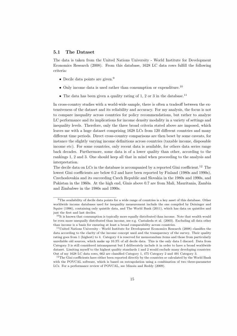
Pareto Density (α = 1.2428)(True) Rohde Density (β =1.1)Chotikapanich Density (k = 6.4609)Lognormal Density (σ =1.4276)Weibull Density (b=0.5814)
Figure 8: Normalized Densities associated with the LCs from Figure (7)
of the domain.8
One can conclude that the relevance of choosing an LC with the correctly implied
modality diminishes in extremely inegalitarian settings. This case, with a simulated Gini
coefficient of 0.6725, is however of limited practical importance. For egalitarian and moder-
ately inegalitarian income distributions, the researcher should definitely take the modality
into account because decile point goodness of fit criteria like MSE and Gini difference can
lead to an LC with an incorrect density shape.
5 An Empirical Analysis
After the MC simulations, let us now turn to empirical data. How do the Pareto, Rohde,
Chotikapanich, Lognormal and Weibull LCs fit countries’ decile income data? How can the
researcher pick an LC associated with correct modality, if the true income density modality
is unknown?
8In a Lognormal density with mean 1 (and therefore µ̄ = −σ2
2), the mode is located at
x̃ = eµ̄−σ2= e−
32σ2
(17)
Using the Gini of the Lognormal Lorenz Curve 2Φ(
σ√2
)− 1, one can express the location of the mode (17)
as a direct function of the Gini coefficient:
x̃ = e−3
[Φ−1
(Gini+1
2
)]2(18)
For a Gini of 0.5, the mode is at 0.2554, while in the above case of a Gini at 0.6725, the mode is at very low
0.0563 - keeping in mind that mean income is still 1.
14
5.1 The Dataset
The data is taken from the United Nations University - World Institute for Development
Economics Research (2008). From this database, 1628 LC data rows fulfill the following
criteria:
• Decile data points are given.9
• Only income data is used rather than consumption or expenditure.10
• The data has been given a quality rating of 1, 2 or 3 in the database.11
In cross-country studies with a world-wide sample, there is often a tradeoff between the ex-
tensiveness of the dataset and its reliability and accuracy. For my analysis, the focus is not
to compare inequality across countries for policy recommendations, but rather to analyze
LC performance and its implications for income density modality in a variety of settings and
inequality levels. Therefore, only the three broad criteria stated above are imposed, which
leaves me with a huge dataset comprising 1628 LCs from 120 different countries and many
different time periods. Direct cross-country comparisons are then beset by some caveats, for
instance the slightly varying income definitions across countries (taxable income, disposable
income etc). For some countries, only recent data is available, for others data series range
back decades. Furthermore, some data is of a lower quality than other, according to the
rankings 1, 2 and 3. One should keep all that in mind when proceeding to the analysis and
interpretation.
The decile data on LCs in the database is accompanied by a reported Gini coefficient.12 The
lowest Gini coefficients are below 0.2 and have been reported by Finland (1980s and 1990s),
Czechoslovakia and its succeeding Czech Republic and Slovakia in the 1980s and 1990s, and
Pakistan in the 1960s. At the high end, Ginis above 0.7 are from Mali, Mauritania, Zambia
and Zimbabwe in the 1980s and 1990s.
9The availability of decile data points for a wide range of countries is a key asset of this database. Other
worldwide income databases used for inequality measurement include the one compiled by Deininger and
Squire (1996), containing only quintile data, and The World Bank (2011), which has data on quintiles and
just the first and last deciles.10It is known that consumption is typically more equally distributed than income. Note that wealth would
be even more unequally distributed than income, see e.g. Castañeda et al. (2003). Excluding all data other
than income is a basis for ensuring at least a broad comparability across countries.11United Nations University - World Institute for Development Economics Research (2008) classifies the
data according to the clarity of the income concept used and the transparency of the survey. Their quality
rating goes from 1 (highest) to 4. Category 4 is reserved for memorandum items and those from particularly
unreliable old sources, which make up 10.3% of all decile data. This is the only data I discard. Data from
Category 3 is still considered intransparent but I deliberately include it in order to have a broad worldwide
dataset. Limiting myself to the highest quality standards 1 and 2 would exclude many developing countries:
Out of my 1628 LC data rows, 662 are classified Category 1, 475 Category 2 and 491 Category 3.12The Gini coefficients have either been reported directly by the countries or calculated by the World Bank
with the POVCAL software, which is based on extrapolation using a combination of two three-parameter
LCs. For a performance review of POVCAL, see Minoiu and Reddy (2009).
15
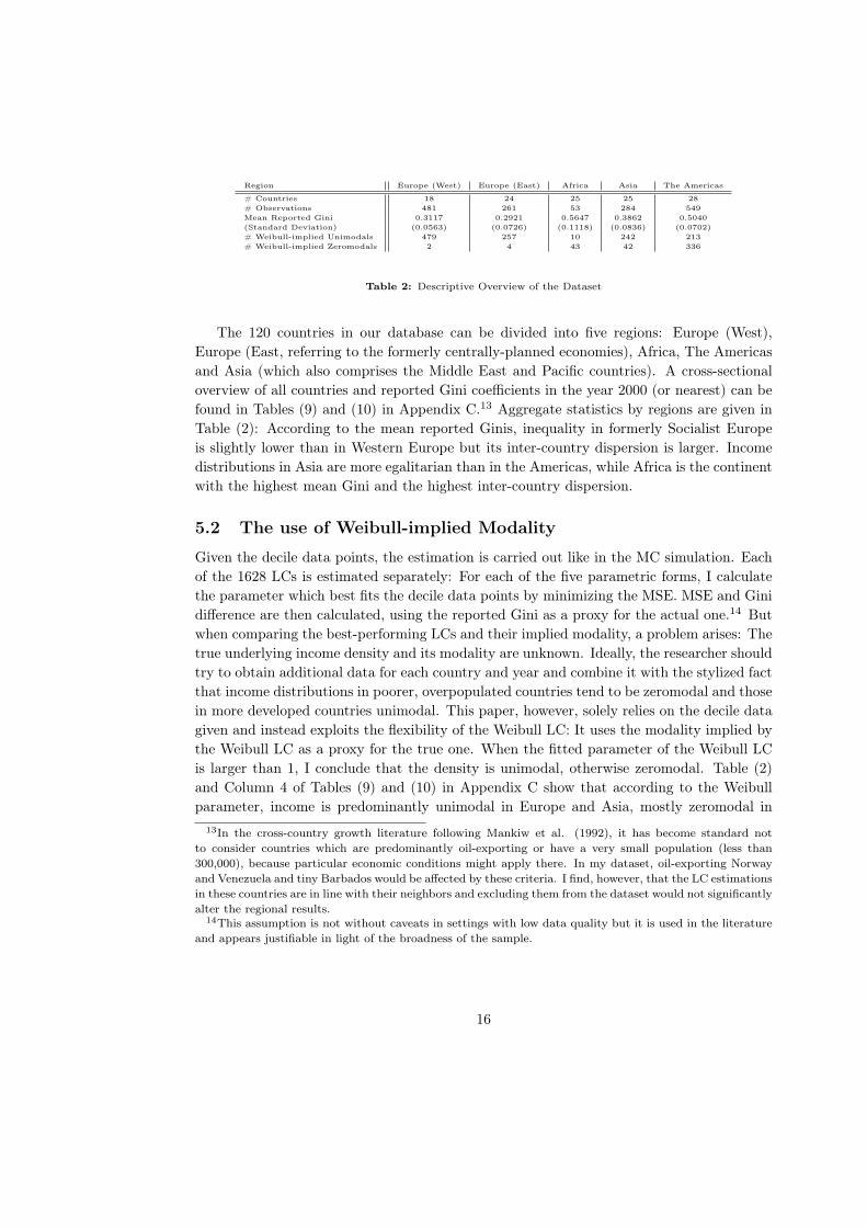
Region Europe (West) Europe (East) Africa Asia The Americas
# Countries 18 24 25 25 28
# Observations 481 261 53 284 549
Mean Reported Gini 0.3117 0.2921 0.5647 0.3862 0.5040
(Standard Deviation) (0.0563) (0.0726) (0.1118) (0.0836) (0.0702)
# Weibull-implied Unimodals 479 257 10 242 213
# Weibull-implied Zeromodals 2 4 43 42 336
Table 2: Descriptive Overview of the Dataset
The 120 countries in our database can be divided into five regions: Europe (West),
Europe (East, referring to the formerly centrally-planned economies), Africa, The Americas
and Asia (which also comprises the Middle East and Pacific countries). A cross-sectional
overview of all countries and reported Gini coefficients in the year 2000 (or nearest) can be
found in Tables (9) and (10) in Appendix C.13 Aggregate statistics by regions are given in
Table (2): According to the mean reported Ginis, inequality in formerly Socialist Europe
is slightly lower than in Western Europe but its inter-country dispersion is larger. Income
distributions in Asia are more egalitarian than in the Americas, while Africa is the continent
with the highest mean Gini and the highest inter-country dispersion.
5.2 The use of Weibull-implied Modality
Given the decile data points, the estimation is carried out like in the MC simulation. Each
of the 1628 LCs is estimated separately: For each of the five parametric forms, I calculate
the parameter which best fits the decile data points by minimizing the MSE. MSE and Gini
difference are then calculated, using the reported Gini as a proxy for the actual one.14 But
when comparing the best-performing LCs and their implied modality, a problem arises: The
true underlying income density and its modality are unknown. Ideally, the researcher should
try to obtain additional data for each country and year and combine it with the stylized fact
that income distributions in poorer, overpopulated countries tend to be zeromodal and those
in more developed countries unimodal. This paper, however, solely relies on the decile data
given and instead exploits the flexibility of the Weibull LC: It uses the modality implied by
the Weibull LC as a proxy for the true one. When the fitted parameter of the Weibull LC
is larger than 1, I conclude that the density is unimodal, otherwise zeromodal. Table (2)
and Column 4 of Tables (9) and (10) in Appendix C show that according to the Weibull
parameter, income is predominantly unimodal in Europe and Asia, mostly zeromodal in
13In the cross-country growth literature following Mankiw et al. (1992), it has become standard not
to consider countries which are predominantly oil-exporting or have a very small population (less than
300,000), because particular economic conditions might apply there. In my dataset, oil-exporting Norway
and Venezuela and tiny Barbados would be affected by these criteria. I find, however, that the LC estimations
in these countries are in line with their neighbors and excluding them from the dataset would not significantly
alter the regional results.14This assumption is not without caveats in settings with low data quality but it is used in the literature
and appears justifiable in light of the broadness of the sample.
16
Africa and sometimes unimodal, sometimes zeromodal on the American continent.15
5.3 Empirical LC Fitting Results, classified by Density Modality
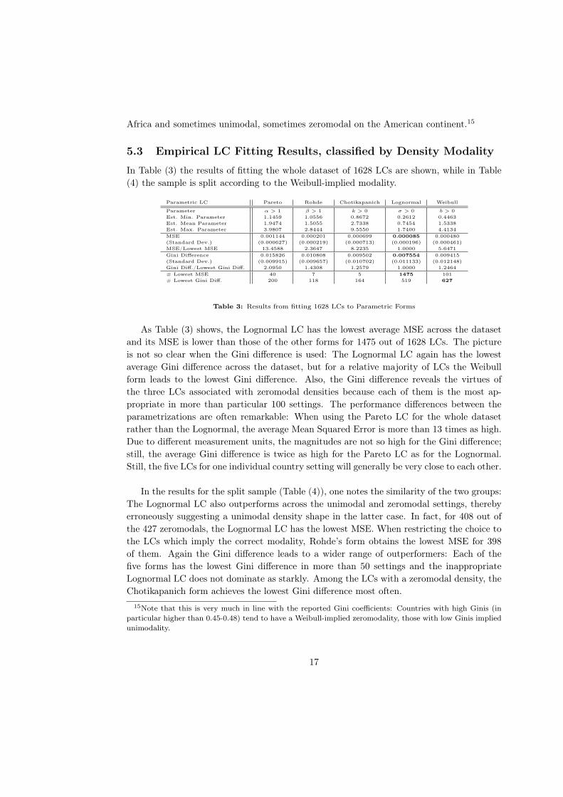
In Table (3) the results of fitting the whole dataset of 1628 LCs are shown, while in Table
(4) the sample is split according to the Weibull-implied modality.
Parametric LC Pareto Rohde Chotikapanich Lognormal Weibull
Parameter α > 1 β > 1 k > 0 σ > 0 b > 0
Est. Min. Parameter 1.1459 1.0556 0.8672 0.2612 0.4463
Est. Mean Parameter 1.9474 1.5055 2.7338 0.7454 1.5338
Est. Max. Parameter 3.9807 2.8444 9.5550 1.7400 4.4134
MSE 0.001144 0.000201 0.000699 0.000085 0.000480
(Standard Dev.) (0.000627) (0.000219) (0.000713) (0.000196) (0.000461)
MSE/Lowest MSE 13.4588 2.3647 8.2235 1.0000 5.6471
Gini Difference 0.015826 0.010808 0.009502 0.007554 0.009415
(Standard Dev.) (0.009915) (0.009657) (0.010702) (0.011133) (0.012148)
Gini Diff./Lowest Gini Diff. 2.0950 1.4308 1.2579 1.0000 1.2464
# Lowest MSE 40 7 5 1475 101
# Lowest Gini Diff. 200 118 164 519 627
Table 3: Results from fitting 1628 LCs to Parametric Forms
As Table (3) shows, the Lognormal LC has the lowest average MSE across the dataset
and its MSE is lower than those of the other forms for 1475 out of 1628 LCs. The picture
is not so clear when the Gini difference is used: The Lognormal LC again has the lowest
average Gini difference across the dataset, but for a relative majority of LCs the Weibull
form leads to the lowest Gini difference. Also, the Gini difference reveals the virtues of
the three LCs associated with zeromodal densities because each of them is the most ap-
propriate in more than particular 100 settings. The performance differences between the
parametrizations are often remarkable: When using the Pareto LC for the whole dataset
rather than the Lognormal, the average Mean Squared Error is more than 13 times as high.
Due to different measurement units, the magnitudes are not so high for the Gini difference;
still, the average Gini difference is twice as high for the Pareto LC as for the Lognormal.
Still, the five LCs for one individual country setting will generally be very close to each other.
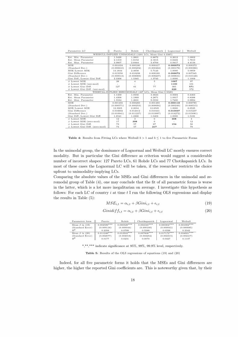
In the results for the split sample (Table (4)), one notes the similarity of the two groups:
The Lognormal LC also outperforms across the unimodal and zeromodal settings, thereby
erroneously suggesting a unimodal density shape in the latter case. In fact, for 408 out of
the 427 zeromodals, the Lognormal LC has the lowest MSE. When restricting the choice to
the LCs which imply the correct modality, Rohde’s form obtains the lowest MSE for 398
of them. Again the Gini difference leads to a wider range of outperformers: Each of the
five forms has the lowest Gini difference in more than 50 settings and the inappropriate
Lognormal LC does not dominate as starkly. Among the LCs with a zeromodal density, the
Chotikapanich form achieves the lowest Gini difference most often.
15Note that this is very much in line with the reported Gini coefficients: Countries with high Ginis (in
particular higher than 0.45-0.48) tend to have a Weibull-implied zeromodality, those with low Ginis implied
unimodality.
17
Parametric LC Pareto Rohde Chotikapanich Lognormal Weibull
WEIBULL-IMPLIED UNIMODALS (1201 LCs, Mean Gini 0.3387)
Est. Min. Parameter 1.5426 1.2601 0.8672 0.2612 1.0002
Est. Mean Parameter 2.1319 1.6152 2.1815 0.6222 1.7810
Est. Max. Parameter 3.9807 2.8444 3.4764 0.9417 4.4134
MSE 0.001034 0.000180 0.000417 0.000073 0.000372
(Standard Dev.) (0.000610) (0.000202) (0.000462) (0.000176) (0.000386)
MSE/Lowest MSE 14.1644 2.4658 5.7123 1.0000 5.0959
Gini Difference 0.015550 0.010238 0.009169 0.006672 0.007345
(Standard Dev.) (0.009513) (0.008969) (0.009237) (0.009631) (0.010148)
Gini Diff./Lowest Gini Diff. 2.3306 1.5345 1.3743 1.0000 1.1009
# Lowest MSE 28 4 5 1067 97
# Lowest MSE (uni-mod) - - - 1100 101
# Lowest Gini Diff. 127 61 77 365 571
# Lowest Gini Diff. (uni-mod) - - - 629 572
WEIBULL-IMPLIED ZEROMODALS (427 LCs, Mean Gini 0.5520)
Est. Min. Parameter 1.1459 1.0556 3.4624 0.9394 0.4463
Est. Mean Parameter 1.4306 1.1969 4.2871 1.0917 0.8388
Est. Max. Parameter 1.5534 1.2631 9.5550 1.7400 0.9994
MSE 0.001455 0.000260 0.001493 0.000118 0.000785
(Standard Dev.) (0.000571) (0.000253) (0.000694) (0.000240) (0.000515)
MSE/Lowest MSE 12.3305 2.2034 12.6525 1.0000 6.6525
Gini Difference 0.016602 0.012412 0.010441 0.010037 0.015237
(Standard Dev.) (0.010941) (0.011227) (0.013997) (0.014272) (0.015081)
Gini Diff./Lowest Gini Diff. 1.6541 1.2366 1.0403 1.0000 1.5181
# Lowest MSE 12 3 0 408 4
# Lowest MSE (zero-mod) 17 398 0 - 12
# Lowest Gini Diff. 73 57 87 154 56
# Lowest Gini Diff. (zero-mod) 74 57 217 - 79
Table 4: Results from Fitting LCs where Weibull b > 1 and b ≤ 1 to five Parametric Forms
In the unimodal group, the dominance of Lognormal and Weibull LC mostly ensures correct
modality. But in particular the Gini difference as criterion would suggest a considerable
number of incorrect shapes: 127 Pareto LCs, 61 Rohde LCs and 77 Chotikapanich LCs. In
most of these cases the Lognormal LC will be taken, if the researcher restricts the choice
upfront to unimodality-implying LCs.
Comparing the absolute values of the MSEs and Gini differences in the unimodal and ze-
romodal group of Table (4), one may conclude that the fit of all parametric forms is worse
in the latter, which is a lot more inegalitarian on average. I investigate this hypothesis as
follows: For each LC of country i at time t I run the following OLS regressions and display
the results in Table (5):
MSEi,t = αi,t + βGinii,t + ǫi,t (19)
Ginidiffi,t = αi,t + βGinii,t + ǫi,t (20)
Parametric form Pareto Rohde Chotikapanich Lognormal Weibull
Mean β in (19) 0.002596∗∗∗ 0.000528∗∗∗ 0.004540∗∗∗ 0.000302∗∗∗ 0.001902∗∗∗
(Standard Error) (0.000116) (0.000044) (0.000100) (0.000041) (0.000085)
R2 0.2356 0.0799 0.5588 0.0326 0.2342
Mean β in (20) 0.011249∗∗∗ 0.012502∗∗∗ 0.007608∗∗∗ 0.017172∗∗∗ 0.034921∗∗∗
(Standard Error) (0.002077) (0.002018) (0.002254) (0.002315) (0.002417)
R2 0.0177 0.0231 0.0070 0.0327 0.1137
*,**,*** indicate significance at 95%, 99%, 99.9% level, respectively.
Table 5: Results of the OLS regressions of equations (19) and (20)
Indeed, for all five parametric forms it holds that the MSEs and Gini differences are
higher, the higher the reported Gini coefficients are. This is noteworthy given that, by their
18
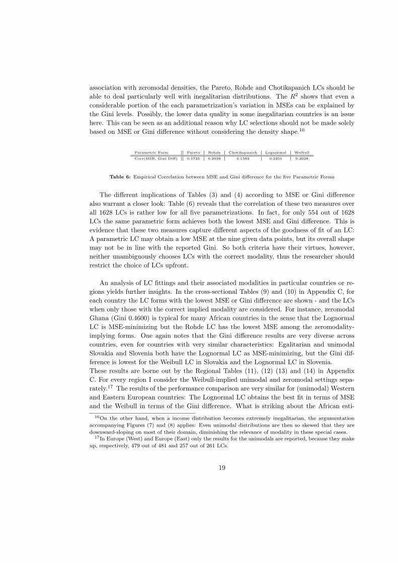
association with zeromodal densities, the Pareto, Rohde and Chotikapanich LCs should be
able to deal particularly well with inegalitarian distributions. The R2 shows that even a
considerable portion of the each parametrization’s variation in MSEs can be explained by
the Gini levels. Possibly, the lower data quality in some inegalitarian countries is an issue
here. This can be seen as an additional reason why LC selections should not be made solely
based on MSE or Gini difference without considering the density shape.16
Parametric Form Pareto Rohde Chotikapanich Lognormal Weibull
Corr(MSE, Gini Diff) 0.1725 0.2039 0.1592 0.2251 0.3028
Table 6: Empirical Correlation between MSE and Gini difference for the five Parametric Forms
The different implications of Tables (3) and (4) according to MSE or Gini difference
also warrant a closer look: Table (6) reveals that the correlation of these two measures over
all 1628 LCs is rather low for all five parametrizations. In fact, for only 554 out of 1628
LCs the same parametric form achieves both the lowest MSE and Gini difference. This is
evidence that these two measures capture different aspects of the goodness of fit of an LC:
A parametric LC may obtain a low MSE at the nine given data points, but its overall shape
may not be in line with the reported Gini. So both criteria have their virtues, however,
neither unambiguously chooses LCs with the correct modality, thus the researcher should
restrict the choice of LCs upfront.
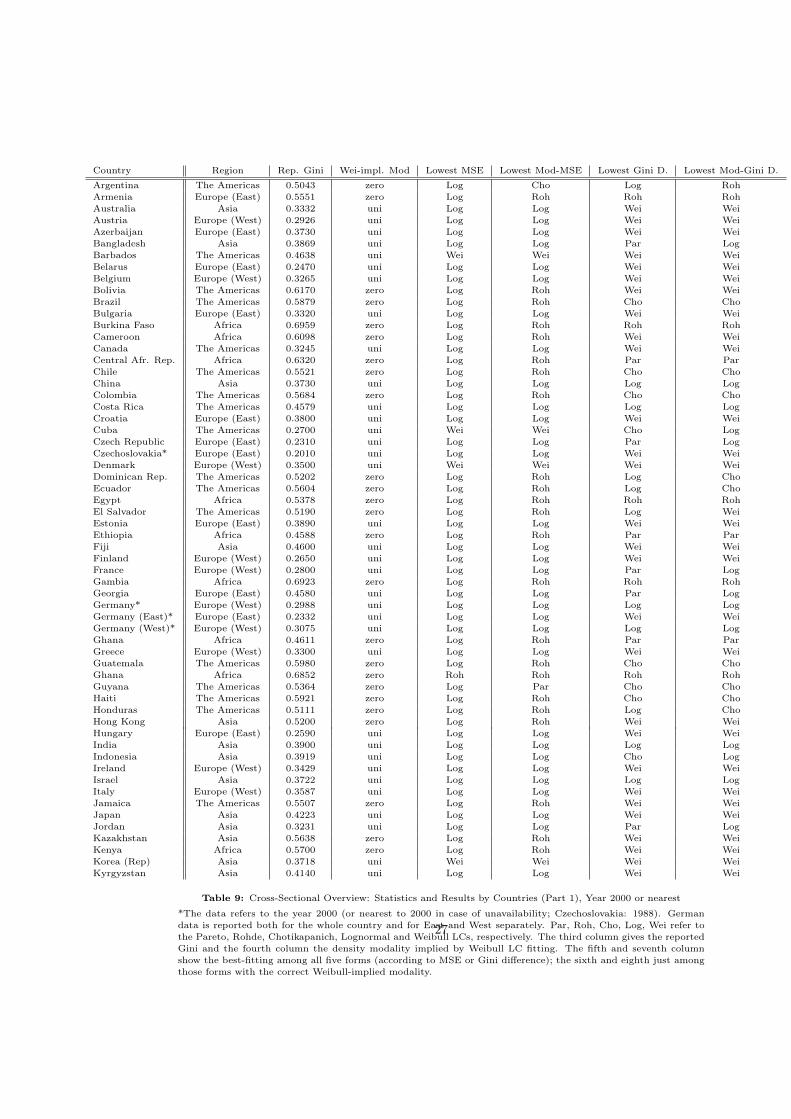
An analysis of LC fittings and their associated modalities in particular countries or re-
gions yields further insights. In the cross-sectional Tables (9) and (10) in Appendix C, for
each country the LC forms with the lowest MSE or Gini difference are shown - and the LCs
when only those with the correct implied modality are considered. For instance, zeromodal
Ghana (Gini 0.4600) is typical for many African countries in the sense that the Lognormal
LC is MSE-minimizing but the Rohde LC has the lowest MSE among the zeromodality-
implying forms. One again notes that the Gini difference results are very diverse across
countries, even for countries with very similar characteristics: Egalitarian and unimodal
Slovakia and Slovenia both have the Lognormal LC as MSE-minimizing, but the Gini dif-
ference is lowest for the Weibull LC in Slovakia and the Lognormal LC in Slovenia.
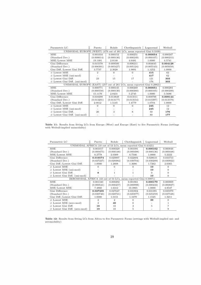
These results are borne out by the Regional Tables (11), (12) (13) and (14) in Appendix
C. For every region I consider the Weibull-implied unimodal and zeromodal settings sepa-
rately.17 The results of the performance comparison are very similar for (unimodal) Western
and Eastern European countries: The Lognormal LC obtains the best fit in terms of MSE
and the Weibull in terms of the Gini difference. What is striking about the African esti-
16On the other hand, when a income distribution becomes extremely inegalitarian, the argumentation
accompanying Figures (7) and (8) applies: Even unimodal distributions are then so skewed that they are
downward-sloping on most of their domain, diminishing the relevance of modality in these special cases.17In Europe (West) and Europe (East) only the results for the unimodals are reported, because they make
up, respectively, 479 out of 481 and 257 out of 261 LCs.
19
mation is that even among the unimodal settings, the Pareto LC achieves the lowest Gini
difference. Only when the unimodality restriction is imposed, the Lognormal LC outper-
forms. It is also noteworthy that the Weibull LC does poorly in the African sample, both in
the zeromodal and unimodal groups: It has the second-highest MSE and the highest Gini
difference of all five forms. And it does not fare much better in Asia and in the Americas.
In Asia, unimodal settings are best captured by the Lognormal LC, while the Pareto and
Rohde forms do well for the zeromodal observations. In the Americas, MSE and Gini differ-
ence point to the Lognormal LC for both groups; after considering modality, Rohde’s and
Chotikapanich’s forms outperform the others in the zeromodal settings.
Outside Europe, the Weibull LC thus mostly does worse than the other forms. Obviously,
its flexibility to encompass unimodal and zeromodal densities - and its ability to give a hint
at the underlying modality - comes at a cost. In many circumstances the other, more spe-
cialized, forms obtain a better fit. The empirical analysis has also shown that once modality
is correctly taken into account the Lognormal LC is the best for most unimodal settings
while the Pareto, Rohde and Chotikapanich forms all have some zeromodal settings where
they do best. The results are generally more mixed with Gini difference rather than MSE
as goodness of fit criterion.
6 Conclusion
This paper has derived a relation between the LC and the modality of its density function.
Given any parametric LC, its third derivative gives an indication of how the underlying
density looks like without having to derive it. Even LCs whose graphs appear similar can
have very different densities, as one can see with the zeromodal Pareto, Chotikapanich and
Rohde forms compared to the unimodal Lognormal and the flexible Weibull.
Both the Monte Carlo simulation and the empirical analysis show that LC fitting based on
MSE or Gini difference can lead to an LC whose density has an incorrect modality. The
resulting implications about the relative numbers of rich, middle-class and poor earners
can thus be highly misleading. This paper therefore argues that researchers should limit
their choice of LCs to those forms associated with the appropriate density modality (e.g. by
checking the third derivative of the LC). In case the shape of the income density is unknown,
more information should be gathered, or the parameter estimate of the best-fitting Weibull
LC can give a hint. Indeed, from our empirical analysis one may conclude that one main
asset of the Weibull LC is indicating the modality, while the other, more specialized, LCs
often obtain lower MSE or Gini differences in most unimodal or zeromodal settings.
Furthermore, the complementarity of the two goodness of fit criteria, MSE and Gini differ-
ence, is worth pointing out. While the MSE focuses on the fit of the curve at the given data
points, the Gini difference takes into account the appropriateness of the overall LC. In my
dataset these two measures have only a weak correlation and frequently lead to different
results. A more thorough investigation into these and alternative goodness of fit criteria
would be interesting for future research.
20
References
Aitchison, J. and J. Brown (1957). The Lognormal Distribution. Cambridge University
Press.
Arnold, B. C. (1983). Pareto Distributions. International Cooperative Publishing House.
Arnold, B. C. (1987). Majorization and the Lorenz Curve: A Brief Introduction. Springer.
Basmann, R., K. Hayes, J. Johnson, and D. Slottje (2002). A General Functional Form
for Approximating the Lorenz Curve. Journal of Econometrics 43, 77–90.
Castañeda, A., J. Díaz-Gimémez, and J.-V. Ríos-Rull (2003). Accounting for the U.S.
Earnings and Wealth Inequality. Journal of Political Economy 111, 818–857.
Chotikapanich, D. (1993). A Comparison of Alternative Functional Forms for the Lorenz
Curve. Economics Letters 41, 129–138.
Cowell, F. and M.-P. Victoria-Feser (2007). Robust Stochastic Dominance: A Semi-
Parametric Approach. Journal of Economic Inequality 5, 21–37.
Dagum, C. (1977). A New Model of Personal Income Distribution: Specification and
Estimation. Economie Appliquée 30, 413–437.
Dagum, C. (1999). A Study on the Distributions of Income, Wealth and Human Capital.
Revue Européenne des Sciences Sociales 113, 231–268.
Deininger, K. and L. Squire (1996). A New Data Set Measuring Income Inequality. The
World Bank Economic Review 10, 565–591.
Gastwirth, J. L. (1971). A General Definition of the Lorenz Curve. Econometrica 39,
1037–1039.
Hasegawa, H. and H. Kozumi (2003). Estimation of Lorenz Curves: A Bayesian Nonpara-
metric Approach. Journal of Econometrics 115, 277–291.
Kakwani, N. and N. Podder (1973). On the Estimation of the Lorenz Curve from Grouped
Observations. International Economic Review 14, 278–292.
Kakwani, N. and N. Podder (1976). Efficient Estimation of the Lorenz Curve and Asso-
ciated Inequality Measures from Grouped Observations. Econometrica 44, 137–149.
Kakwani, N. C. (1980). Income Inequality and Poverty: Methods of Estimation and Policy
Applications. Oxford University Press.
Kleiber, C. (2008). A Guide to the Dagum Distribution. In D. Chotikapanich (Ed.),
Modeling Income Distributions and Lorenz Curves (Economic Studies in Inequality),
pp. 97–117. Springer.
Kullback, S. and R. Leibler (1951). On Information and Sufficiency. Annals of Mathemat-
ical Statistics 22, 79–86.
Lorenz, M. O. (1905). Methods of Measuring the Concentration of Wealth. Publications
of the American Statistical Association 9, 209–219.
21
Mankiw, N. G., D. Romer, and D. N. Weil (1992). A Contribution to the Empirics of
Economic Growth. The Quarterly Journal of Economics 107, 407–437.
McDonald, J. B. (1984). Some Generalized Functions for the Size Distribution of Income.
Econometrica 52, 647–663.
McDonald, J. B. and M. Ransom (2008). The Generalized Beta Distribution as a Model
for the Distribution of Income: Estimation of Related Measures of Inequality. In
D. Chotikapanich (Ed.), Modeling Income Distributions and Lorenz Curves (Economic
Studies in Inequality), pp. 147–166. Springer.
Minoiu, C. and S. G. Reddy (2009). Estimating Poverty and Inequality from Grouped
Data: How Well Do Parametric Methods Perform? Journal of Income Distribution 18,
160–178.
Rohde, N. (2009). An Alternative Functional Form for Estimating the Lorenz Curve.
Economics Letters 100, 61–63.
Ryu, H. K. and D. J. Slottje (1999). Parametric Approximations of the Lorenz Curve. In
J. Silber (Ed.), Handbook of Income Inequality Measurement, pp. 291–314. Springer.
Sarabia, J. M. (2008). Parametric Lorenz Curves: Models and Applications. In
D. Chotikapanich (Ed.), Modeling Income Distributions and Lorenz Curves (Economic
Studies in Inequality), pp. 167–190. Springer.
The World Bank (2011). Distribution of Income and Consumption. World Development
Indicators.
United Nations University - World Institute for Development Economics Research (2008).
UNU-WIDER World Income Inequality Database. Version 2.0c.
Villasenor, J. and B. Arnold (1989). Elliptical Lorenz Curves. Journal of Econometrics 40,
327–338.
7 Appendix
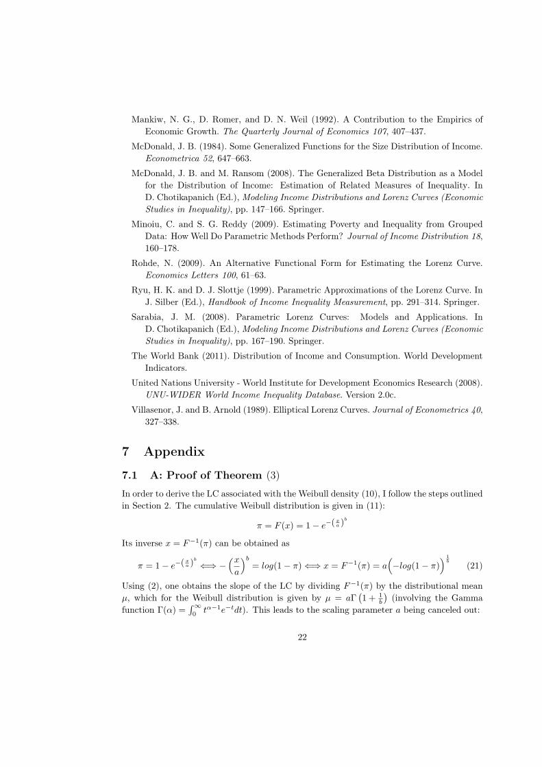
7.1 A: Proof of Theorem (3)
In order to derive the LC associated with the Weibull density (10), I follow the steps outlined
in Section 2. The cumulative Weibull distribution is given in (11):
π = F (x) = 1− e−(xa )
b
Its inverse x = F−1(π) can be obtained as
π = 1− e−(xa )
b
⇐⇒ −(xa
)b
= log(1− π) ⇐⇒ x = F−1(π) = a(−log(1− π)
) 1b
(21)
Using (2), one obtains the slope of the LC by dividing F−1(π) by the distributional mean
µ, which for the Weibull distribution is given by µ = aΓ(1 + 1
b
)(involving the Gamma
function Γ(α) =∫∞
0tα−1e−tdt). This leads to the scaling parameter a being canceled out:
22
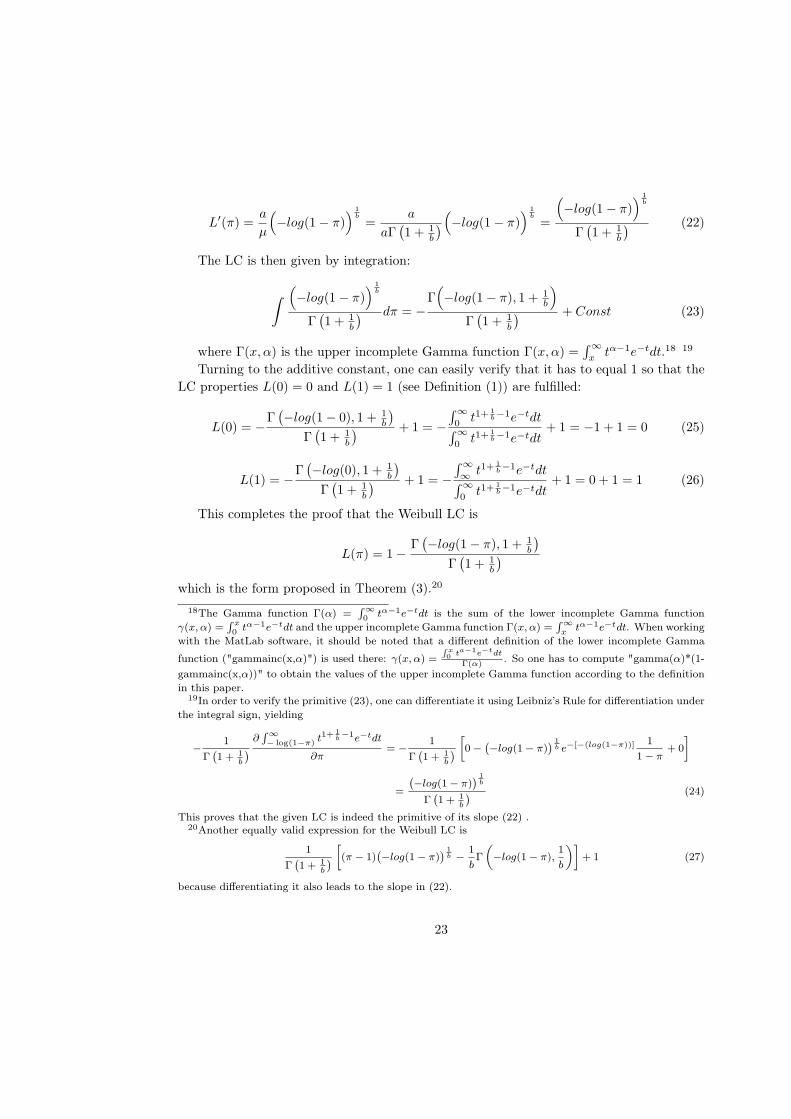
L′(π) =a
µ
(−log(1− π)
) 1b
=a
aΓ(1 + 1
b
)(−log(1− π)
) 1b
=
(−log(1− π)
) 1b
Γ(1 + 1
b
) (22)
The LC is then given by integration:
∫(−log(1− π)
) 1b
Γ(1 + 1
b
) dπ = −Γ(−log(1− π), 1 + 1
b
)
Γ(1 + 1
b
) + Const (23)
where Γ(x, α) is the upper incomplete Gamma function Γ(x, α) =∫∞
xtα−1e−tdt.18 19
Turning to the additive constant, one can easily verify that it has to equal 1 so that the
LC properties L(0) = 0 and L(1) = 1 (see Definition (1)) are fulfilled:
L(0) = −Γ(−log(1− 0), 1 + 1
b
)
Γ(1 + 1
b
) + 1 = −∫∞
0t1+
1b−1e−tdt
∫∞
0t1+
1b−1e−tdt
+ 1 = −1 + 1 = 0 (25)
L(1) = −Γ(−log(0), 1 + 1
b
)
Γ(1 + 1
b
) + 1 = −∫∞
∞t1+
1b−1e−tdt
∫∞
0t1+
1b−1e−tdt
+ 1 = 0 + 1 = 1 (26)
This completes the proof that the Weibull LC is
L(π) = 1− Γ(−log(1− π), 1 + 1
b
)
Γ(1 + 1
b
)
which is the form proposed in Theorem (3).20
18The Gamma function Γ(α) =∫∞0 tα−1e−tdt is the sum of the lower incomplete Gamma function
γ(x, α) =∫ x
0 tα−1e−tdt and the upper incomplete Gamma function Γ(x, α) =∫∞x
tα−1e−tdt. When working
with the MatLab software, it should be noted that a different definition of the lower incomplete Gamma
function ("gammainc(x,α)") is used there: γ(x, α) =∫x0 ta−1e−tdt
Γ(α). So one has to compute "gamma(α)*(1-
gammainc(x,α))" to obtain the values of the upper incomplete Gamma function according to the definition
in this paper.19In order to verify the primitive (23), one can differentiate it using Leibniz’s Rule for differentiation under
the integral sign, yielding
−1
Γ(1 + 1
b
)∂∫∞− log(1−π) t
1+ 1b−1e−tdt
∂π= −
1
Γ(1 + 1
b
)[0−
(−log(1− π)
) 1b e−[−(log(1−π))] 1
1− π+ 0
]
=
(−log(1− π)
) 1b
Γ(1 + 1
b
) (24)
This proves that the given LC is indeed the primitive of its slope (22) .20Another equally valid expression for the Weibull LC is
1
Γ(1 + 1
b
)[(π − 1)
(−log(1− π)
) 1b −
1
bΓ
(−log(1− π),
1
b
)]+ 1 (27)
because differentiating it also leads to the slope in (22).
23
7.2 B: Analysis of the Weibull LC’s third derivative (13)
The first three derivatives of the Weibull LC (12) are
L′(π) =
(−log(1− π)
) 1b
Γ(1 + 1
b
) ; L′′(π) =
(−log(1− π)
) 1b−1
Γ(1 + 1
b
)b(1− π)
(28)
L′′′(π) =
(−log(1− π)
) 1b−2
Γ(1 + 1
b
)b2(1− π)2
[1− b+ b
(−log(1− π)
)](29)
From Theorem (2) it directly follows that L′′′(π) is positive for b ≤ 1, implying a ze-
romodal density, and sign-changing for b > 1, implying a unimodal density. In the latter
case, L′′′(π) = 0 occurs at the point π̃ referring to the mode x̃ = a(1− 1
b
) 1b of the Weibull
density.
One can, however, also verify these properties without relying on Theorem (2), by looking
at (29): Recall that b > 0 and 0 ≤ π ≤ 1, so the ratio in (29) is unambiguously positive. It
is the term in square brackets which determines the sign of L′′′(π): For 0 < b ≤ 1, this term
is positive as well and hence, the third derivative is positive. By (5), f ′(x) is then negative
for all x, which corresponds to the zeromodality of the Weibull density for 0 < b ≤ 1. On
the other hand, if b > 1, the term in square brackets can become negative:
1− b+ b(−log(1− π)
)< 0 ⇐⇒ π < π̃ = 1− e
1b−1 (30)
In the case of a unimodal Weibull density, the third derivative of the LC is negative for
π below a threshold value π̃, referring to the upward-sloping part of the density. The more
concentrated the Weibull density (thus the higher b), the higher this threshold because the
higher the mode. In fact, the change from a negative to a positive third LC derivative occurs
just at the Weibull mode x̃ = a(1− 1
b
) 1b :
1− b+ b(−log(1− 1 + e−(
x̃a )
b
))= 0 ⇐⇒ x̃ = a
(1− 1
b
) 1b
(31)
This completes the proof.
7.3 C: Large Tables
24
Parametric LC Pareto Rohde Chotikapanich Lognormal Weibull
Density Modality zero zero zero uni zero/uni
Parameter α > 1 β > 1 k > 0 b > 0 σ > 0
WEIBULL with b = 3 (unimodal, Gini 0.2063)
Est. Mean Parameter 3.0976 2.2010 1.2372 0.3653 3.0007
(Standard Dev.) (0.0187) (0.0120) (0.0096) (0.0027) (0.0249)
MSE 0.000995 0.000142 0.000073 0.000110 0.000000
(Standard Dev.) (0.000024) (0.000007) (0.000004) (0.000007) (0.000000)
Gini Difference 0.013807 0.006809 0.005177 0.002543 0.001218
(Standard Dev.) (0.001389) (0.001455) (0.001485) (0.001375) (0.000918)
K-L Distance 7.5213 4.5157 4.0850 0.3215 0.0002
Integral Diff. 0.8367 0.4829 0.4249 0.2510 0.0002
WEIBULL with b = 1.5 (unimodal, Gini 0.3700)
Est. Mean Parameter 1.9460 1.4885 2.3695 0.6701 1.5002
(Standard Dev.) (0.0094) (0.0056) (0.0183) (0.0046) (0.0122)
MSE 0.002647 0.000346 0.000092 0.000277 0.000000
(Standard Dev.) (0.000055) (0.000016) (0.000004) (0.000017) (0.000000)
Gini Difference 0.024251 0.013346 0.007750 0.005665 0.001890
(Standard Dev.) (0.002252) (0.002274) (0.002346) (0.002295) (0.001425)
K-L Distance 9.4520 5.8783 4.5657 0.3803 0.0001
Integral Diff. 0.8935 0.5254 0.4161 0.2563 0.0001
WEIBULL with b = 0.5 (zeromodal, Gini 0.7500)
Est. Mean Parameter 1.1771 1.0722 7.9695 1.6074 0.5002
(Standard Dev.) (0.0040) (0.0018) (0.1295) (0.0136) (0.0056)
MSE 0.003299 0.000459 0.000462 0.000303 0.000001
(Standard Dev.) (0.000122) (0.000031) (0.000037) (0.000031) (0.000001)
Gini Difference 0.011570 0.023295 0.003186 0.006033 0.003116
(Standard Dev.) (0.004371) (0.003982) (0.002415) (0.003574) (0.002363)
K-L Distance 25.3942 21.1329 12.7451 5.4718 0.0010
Integral Diff. 1.3470 0.9523 0.6593 0.5500 0.0010
LOGNORMAL with σ = 0.4 (unimodal, Gini 0.2227)
Est. Mean Parameter 2.8449 2.0608 1.3511 0.4000 2.7339
(Standard Dev.) (0.0176) (0.0111) (0.0106) (0.0030) (0.0231)
MSE 0.000534 0.000037 0.000065 0.000000 0.000127
(Standard Dev.) (0.000016) (0.000002) (0.000005) (0.000000) (0.000008)
Gini Difference 0.009462 0.004536 0.004096 0.001321 0.001689
(Standard Dev.) (0.001600) (0.001616) (0.001609) (0.000992) (0.001224)
K-L Distance 7.1015 3.7911 3.3431 0.0001 0.2722
Integral Diff. 0.6738 0.3922 0.3880 0.0001 0.2529
LOGNORMAL with σ = 0.8 (unimodal, Gini 0.4284)
Est. Mean Parameter 1.7162 1.3574 2.8746 0.8000 1.2180
(Standard Dev.) (0.0103) (0.0059) (0.0300) (0.0072) (0.0134)
MSE 0.001532 0.000098 0.000449 0.000001 0.000337
(Standard Dev.) (0.000048) (0.000007) (0.000036) (0.000001) (0.000027)
Gini Difference 0.017261 0.008374 0.004837 0.002781 0.005762
(Standard Dev.) (0.003466) (0.003387) (0.003005) (0.002094) 0.003255
K-L Distance 9.1313 4.4648 2.6921 0.0001 0.2440
Integral Diff. 0.7534 0.4185 0.4078 0.0001 0.2632
LOGNORMAL with σ = 1.5 (unimodal, Gini 0.7112)
Est. Mean Parameter 1.2146 1.0874 7.0251 1.4994 0.5464
(Standard Dev.) (0.0075) (0.0035) (0.1879) (0.0216) 0.0105
MSE 0.001797 0.000077 0.001465 0.000001 0.000339
(Standard Dev.) (0.000113) (0.000006) (0.000088) (0.000002) (0.000035)
Gini Difference 0.011858 0.015570 0.007375 0.005470 0.008452
(Standard Dev.) (0.006513) (0.006530) (0.005557) (0.004258) 0.005834
K-L Distance 12.9917 6.9790 1.2474 0.0006 0.2649
Integral Diff. 0.9196 0.5018 0.5525 0.0006 0.8313
Table 7: MC simulation with Weibull- and Lognormally-distributed income data
*Printed in italics are the results for the LC form associated with the sampled density; printed in bold are the
results for best-performing LC apart from this one.
25
Parametric LC Pareto Rohde Chotikapanich Lognormal Weibull
Density Modality zero zero zero uni zero/uni
Parameter α > 1 β > 1 k > 0 b > 0 σ > 0
CHOTIKAPANICH with k = 1.5 (zeromodal, Gini 0.2411)
Est. Mean Parameter 2.6629 1.9289 1.4997 0.4393 2.4466
(Standard Dev.) (0.0100) (0.0063) 0.0076 (0.0021) 0.0132
MSE 0.001058 0.000039 0.000000 0.000085 0.000084
(Standard Dev.) (0.000024) (0.000005) (0.000000) (0.000006) 0.000005
Gini Difference 0.009927 0.001834 0.000905 0.002820 0.005621
(Standard Dev.) (0.001073) (0.001028) (0.000682) (0.001120) (0.001154)
K-L Distance 9.5512 2.8658 0.0078 0.3666 0.3795
Integral Diff. 0.8664 0.2753 0.0004 0.3645 0.4133
CHOTIKAPANICH with k = 6 (zeromodal, Gini 0.6716)
Est. Mean Parameter 1.2680 1.1150 5.9987 1.3620 0.6212
(Standard Dev.) (0.0036) (0.0017) (0.05608) (0.0079) 0.0047
MSE 0.006386 0.001389 0.000001 0.001395 0.000364
(Standard Dev.) (0.000134) (0.000058) (0.000001) (0.000061) (0.000031)
Gini Difference 0.020642 0.024198 0.002263 0.007174 0.002291
(Standard Dev.) (0.003068) (0.002756) (0.001714) (0.007174) (0.002291)
K-L Distance 17.0014 12.4387 0.0013 0.6279 0.3892
Integral Diff. 1.2194 0.7960 0.0003 0.5016 0.4134
ROHDE with β = 2 (zeromodal, Gini 0.2274)
Est. Mean Parameter 2.7622 2.0003 1.4132 0.4165 2.6085
(Standard Dev.) (0.0105) (0.0068) (0.0072) (0.0020) (0.0142)
MSE 0.000652 0.000000 0.000031 0.000039 0.000176
(Standard Dev.) (0.000019) (0.000000) (0.000004) (0.000002) 0.000008
Gini Difference 0.006378 0.000858 0.001019 0.004195 0.005946
(Standard Dev.) (0.001022) (0.000648) (0.000744) (0.001085) (0.001112)
K-L Distance 8.8778 0.0073 1.3711 0.3537 0.4619
Integral Diff. 0.7665 0.0003 0.2602 0.3757 0.4880
ROHDE with β = 1.1 (zeromodal, Gini 0.6725)
Est. Mean Parameter 1.2428 1.1000 6.4609 1.4276 0.5814
(Standard Dev.) (0.0036) (0.0017) (0.0729) (0.0091) 0.0049
MSE 0.001730 0.000001 0.001475 0.000084 0.000503
(Standard Dev.) (0.000080) (0.000001) (0.000071) (0.000005) (0.000034)
Gini Difference 0.002646 0.002377 0.021085 0.014771 0.024003
(Standard Dev.) (0.002013) (0.001815) (0.003267) (0.003077) (0.003052)
K-L Distance 13.4991 0.0008 1.6146 0.4092 0.5860
Integral Diff. 0.9072 0.0002 0.8571 0.4850 0.7034
PARETO with α = 2.5 (zeromodal, Gini 0.2500)
Est. Mean Parameter 2.5015 1.8778 1.5277 0.4574 2.3918
(Standard Dev.) (0.0439) (0.0284) (0.0357) (0.0105) (0.0607)
MSE 0.000000 0.000790 0.001175 0.000692 0.001500
(Standard Dev.) (0.000001) (0.000065) (0.000097) (0.000057) (0.000100)
Gini Difference 0.004301 0.004429 0.005958 0.005108 0.004448
(Standard Dev.) (0.003536) (0.003492) (0.003942) (0.004284) 0.003799
K-L Distance 0.0402 1.9287 2.3998 0.6723 1.1494
Integral Diff. 0.0021 0.7803 0.8790 0.6811 0.8566
PARETO with α = 1.3 (zeromodal, Gini 0.6250)
Est. Mean Parameter 1.3292 1.1407 5.2534 1.2554 0.6971
(Standard Dev.) (0.0563) (0.0284) (1.6184) (0.1481) (0.0817)
MSE 0.000004 0.001823 0.005817 0.001855 0.003940
(Standard Dev.) (0.000005) (0.000153) (0.000566) (0.000153) (0.000293)
Gini Difference 0.039792 0.035512 0.037353 0.032828 0.031848
(Standard Dev.) (0.031952) (0.031415) (0.035946) (0.033818) (0.036224)
K-L Distance 2.9041 0.9601 1.6448 0.7854 1.0591
K-L Distance 0.1641 0.8624 1.1855 0.8491 1.2143
Table 8: MC simulation with Chotikapanich-, Rohde- and Pareto-distributed income data
*Printed in italics are the results for the LC form associated with the sampled density; printed in bold are the
results for best-performing LC apart from this one.
26
Country Region Rep. Gini Wei-impl. Mod Lowest MSE Lowest Mod-MSE Lowest Gini D. Lowest Mod-Gini D.
Argentina The Americas 0.5043 zero Log Cho Log Roh
Armenia Europe (East) 0.5551 zero Log Roh Roh Roh
Australia Asia 0.3332 uni Log Log Wei Wei
Austria Europe (West) 0.2926 uni Log Log Wei Wei
Azerbaijan Europe (East) 0.3730 uni Log Log Wei Wei
Bangladesh Asia 0.3869 uni Log Log Par Log
Barbados The Americas 0.4638 uni Wei Wei Wei Wei
Belarus Europe (East) 0.2470 uni Log Log Wei Wei
Belgium Europe (West) 0.3265 uni Log Log Wei Wei
Bolivia The Americas 0.6170 zero Log Roh Wei Wei
Brazil The Americas 0.5879 zero Log Roh Cho Cho
Bulgaria Europe (East) 0.3320 uni Log Log Wei Wei
Burkina Faso Africa 0.6959 zero Log Roh Roh Roh
Cameroon Africa 0.6098 zero Log Roh Wei Wei
Canada The Americas 0.3245 uni Log Log Wei Wei
Central Afr. Rep. Africa 0.6320 zero Log Roh Par Par
Chile The Americas 0.5521 zero Log Roh Cho Cho
China Asia 0.3730 uni Log Log Log Log
Colombia The Americas 0.5684 zero Log Roh Cho Cho
Costa Rica The Americas 0.4579 uni Log Log Log Log
Croatia Europe (East) 0.3800 uni Log Log Wei Wei
Cuba The Americas 0.2700 uni Wei Wei Cho Log
Czech Republic Europe (East) 0.2310 uni Log Log Par Log
Czechoslovakia* Europe (East) 0.2010 uni Log Log Wei Wei
Denmark Europe (West) 0.3500 uni Wei Wei Wei Wei
Dominican Rep. The Americas 0.5202 zero Log Roh Log Cho
Ecuador The Americas 0.5604 zero Log Roh Log Cho
Egypt Africa 0.5378 zero Log Roh Roh Roh
El Salvador The Americas 0.5190 zero Log Roh Log Wei
Estonia Europe (East) 0.3890 uni Log Log Wei Wei
Ethiopia Africa 0.4588 zero Log Roh Par Par
Fiji Asia 0.4600 uni Log Log Wei Wei
Finland Europe (West) 0.2650 uni Log Log Wei Wei
France Europe (West) 0.2800 uni Log Log Par Log
Gambia Africa 0.6923 zero Log Roh Roh Roh
Georgia Europe (East) 0.4580 uni Log Log Par Log
Germany* Europe (West) 0.2988 uni Log Log Log Log
Germany (East)* Europe (East) 0.2332 uni Log Log Wei Wei
Germany (West)* Europe (West) 0.3075 uni Log Log Log Log
Ghana Africa 0.4611 zero Log Roh Par Par
Greece Europe (West) 0.3300 uni Log Log Wei Wei
Guatemala The Americas 0.5980 zero Log Roh Cho Cho
Ghana Africa 0.6852 zero Roh Roh Roh Roh
Guyana The Americas 0.5364 zero Log Par Cho Cho
Haiti The Americas 0.5921 zero Log Roh Cho Cho
Honduras The Americas 0.5111 zero Log Roh Log Cho
Hong Kong Asia 0.5200 zero Log Roh Wei Wei
Hungary Europe (East) 0.2590 uni Log Log Wei Wei
India Asia 0.3900 uni Log Log Log Log
Indonesia Asia 0.3919 uni Log Log Cho Log
Ireland Europe (West) 0.3429 uni Log Log Wei Wei
Israel Asia 0.3722 uni Log Log Log Log
Italy Europe (West) 0.3587 uni Log Log Wei Wei
Jamaica The Americas 0.5507 zero Log Roh Wei Wei
Japan Asia 0.4223 uni Log Log Wei Wei
Jordan Asia 0.3231 uni Log Log Par Log
Kazakhstan Asia 0.5638 zero Log Roh Wei Wei
Kenya Africa 0.5700 zero Log Roh Wei Wei
Korea (Rep) Asia 0.3718 uni Wei Wei Wei Wei
Kyrgyzstan Asia 0.4140 uni Log Log Wei Wei
Table 9: Cross-Sectional Overview: Statistics and Results by Countries (Part 1), Year 2000 or nearest
*The data refers to the year 2000 (or nearest to 2000 in case of unavailability; Czechoslovakia: 1988). German
data is reported both for the whole country and for East and West separately. Par, Roh, Cho, Log, Wei refer to
the Pareto, Rohde, Chotikapanich, Lognormal and Weibull LCs, respectively. The third column gives the reported
Gini and the fourth column the density modality implied by Weibull LC fitting. The fifth and seventh column
show the best-fitting among all five forms (according to MSE or Gini difference); the sixth and eighth just among
those forms with the correct Weibull-implied modality.
27
Country Region Rep. Gini Wei-impl. Mod Lowest MSE Lowest Mod-MSE Lowest Gini D. Lowest Mod-Gini D.
Latvia Europe (East) 0.3270 uni Log Log Par Log
Lesotho Africa 0.6850 zero Log Roh Log Par
Lithuania Europe (East) 0.3550 uni Log Log Wei Wei
Luxembourg Europe (West) 0.3029 uni Log Log Log Log
Macedonia Europe (East) 0.3460 uni Wei Wei Wei Wei
Madagascar Africa 0.5950 zero Log Roh Par Par
Malawi Africa 0.5670 zero Log Roh Par Par
Malaysia Asia 0.4848 zero Log Roh Par Par
Mali Africa 0.7862 zero Log Roh Wei Wei
Mauritania Africa 0.6908 zero Log Roh Roh Roh
Mexico The Americas 0.5325 zero Log Roh Log Cho
Moldova Europe (East) 0.4214 uni Log Log Log Log
Morocco Africa 0.5240 zero Roh Roh Par Par
Myanmar Asia 0.3806 zero Roh Log Cho Log
Nepal Asia 0.5046 zero Log Roh Par Par
Netherlands Europe (West) 0.2500 uni Log Log Wei Wei
New Zealand Asia 0.4040 uni Log Log Wei Wei
Nicaragua The Americas 0.5442 zero Log Roh Log Cho
Nigeria Africa 0.5290 zero Log Roh Log Wei
Norway Europe (West) 0.2890 uni Log Log Wei Wei
Pakistan Asia 0.3600 uni Log Log Par Log
Panama The Americas 0.5705 zero Log Roh Roh Roh
Paraguay The Americas 0.56925 zero Log Roh Log Wei
Peru The Americas 0.4962 zero Log Roh Log Wei
Philippines Asia 0.4818 zero Log Roh Par Par
Poland Europe (East) 0.3450 uni Log Log Wei Wei
Portugal Europe (West) 0.3600 uni Log Log Wei Wei
Puerto Rico The Americas 0.3970 zero Log Log Log Log
Romania Europe (East) 0.3100 uni Log Log Wei Wei
Russia Europe (East) 0.4262 uni Log Log Wei Wei
Senegal Africa 0.6117 zero Log Roh Roh Roh
Serbia & Monten. Europe (East) 0.3730 uni Log Log Wei Wei
Sierra Leone Africa 0.4400 uni Log Log Par Log
Slovakia Europe (East) 0.2640 uni Log Log Wei Wei
Slovenia Europe (East) 0.2460 uni Log Log Log Log
Somalia Africa 0.3970 uni Log Log Par Log
South Africa Africa 0.5452 zero Par Par Par Par
Spain Europe (West) 0.3458 uni Log Log Wei Wei
Sri Lanka Asia 0.5665 zero Par Par Par Par
Sudan Africa 0.3980 uni Log Log Cho Log
Suriname The Americas 0.5381 zero Log Roh Log Cho
Sweden Europe (West) 0.2950 uni Log Log Wei Wei
Switzerland Europe (West) 0.3596 uni Log Log Wei Wei
Taiwan Asia 0.3194 uni Log Log Log Log
Tanzania Africa 0.5973 zero Log Roh Log Cho
Thailand Asia 0.5595 zero Log Roh Par Par
Trinidad & Tob. The Americas 0.4027 uni Log Log Log Log
Turkey Asia 0.5679 zero Log Roh Log Cho
Turkmenistan Asia 0.3580 uni Log Log Log Log
Uganda Africa 0.5363 zero Log Roh Par Par
Ukraine Europe (East) 0.4916 zero Log Roh Cho Cho
United Kingdom Europe (West) 0.3459 uni Log Log Wei Wei
United States The Americas 0.4019 uni Log Log Wei Wei
Uruguay The Americas 0.4430 uni Log Log Log Log
USSR* Europe (East) 0.2890 uni Log Log Wei Wei
Uzbekistan Asia 0.4717 uni Log Log Roh Log
Venezuela The Americas 0.4410 uni Log Log Log Log
Yugoslavia* Europe (East) 0.3300 uni Wei Wei Wei Wei
Zambia Africa 0.6473 zero Log Roh Par Par
Zimbabwe Africa 0.7461 zero Log Roh Wei Wei
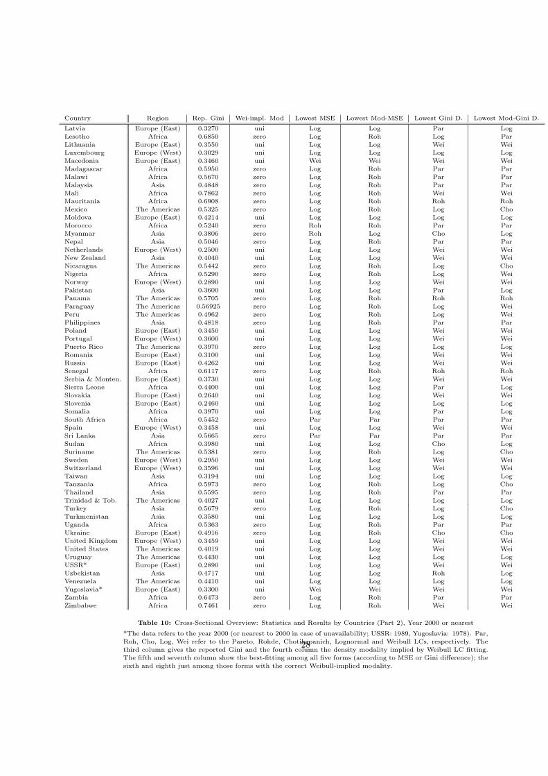
Table 10: Cross-Sectional Overview: Statistics and Results by Countries (Part 2), Year 2000 or nearest
*The data refers to the year 2000 (or nearest to 2000 in case of unavailability; USSR: 1989, Yugoslavia: 1978). Par,
Roh, Cho, Log, Wei refer to the Pareto, Rohde, Chotikapanich, Lognormal and Weibull LCs, respectively. The
third column gives the reported Gini and the fourth column the density modality implied by Weibull LC fitting.
The fifth and seventh column show the best-fitting among all five forms (according to MSE or Gini difference); the
sixth and eighth just among those forms with the correct Weibull-implied modality.
28
Parametric LC Pareto Rohde Chotikapanich Lognormal Weibull
UNIMODAL EUROPE (WEST) (479 out of 481 LCs, mean reported Gini 0.3109)
MSE 0.001034 0.000152 0.000251 0.000054 0.000247
(Standard Dev.) (0.000614) (0.000136) (0.000249) (0.000107) (0.000215)
MSE/Lowest MSE 19.1481 2.8148 4.6481 1.0000 4.5741
Gini Difference 0.015578 0.009506 0.008211 0.004645 0.004128
(Standard Dev.) (0.006301) (0.005427) (0.005124) (0.005543) (0.005659)
Gini Diff./Lowest Gini Diff. 3.7737 2.3028 1.9891 1.1252 1.0000
# Lowest MSE 2 0 0 415 62
# Lowest MSE (uni-mod) - - - 417 62
# Lowest Gini Diff. 23 15 17 121 303
# Lowest Gini Diff. (uni-mod) - - - 176 303
UNIMODAL EUROPE (EAST) (257 out of 261 LCs, mean reported Gini 0.2882))
MSE 0.000771 0.000145 0.000269 0.000051 0.000284
(Standard Dev.) (0.000558) (0.000130) (0.000260) (0.000105) (0.000209)
MSE/Lowest MSE 15.1176 2.8431 5.2745 1.0000 5.5686
Gini Difference 0.018299 0.013849 0.013511 0.009788 0.009144
(Standard Dev.) (0.013201) (0.013177) (0.013554) (0.013397) (0.013579)
Gini Diff./Lowest Gini Diff. 2.0012 1.5145 1.4779 1.0704 1.0000
# Lowest MSE 0 0 0 245 12
# Lowest MSE (uni-mod) - - - 245 12
# Lowest Gini Diff. 20 3 8 50 176
# Lowest Gini Diff. (uni-mod) - - - 80 177
Table 11: Results from fitting LCs from Europe (West) and Europe (East) to five Parametric Forms (settings
with Weibull-implied unimodality)
Parametric LC Pareto Rohde Chotikapanich Lognormal Weibull
UNIMODAL AFRICA (10 out of 53 LCs, mean reported Gini 0.4142))
MSE 0.001017 0.000329 0.001091 0.000162 0.000846
(Standard Dev.) (0.000475) (0.000148) (0.000498) (0.000136) (0.000448)
MSE/Lowest MSE 6.2778 2.0309 6.7346 1.0000 5.2222
Gini Difference 0.016574 0.020897 0.022684 0.028610 0.033753
(Standard Dev.) (0.027227) (0.029384) (0.030704) (0.030209) (0.030922)
Gini Diff./Lowest Gini Diff. 1.0000 1.2608 1.3686 1.7262 2.0365
# Lowest MSE 0 0 0 10 0
# Lowest MSE (uni-mod) - - - 10 0
# Lowest Gini Diff. 8 1 1 0 0
# Lowest Gini Diff. (uni-mod) - - - 10 0
ZEROMODAL AFRICA (43 out of 53 LCs, mean reported Gini 0.5997))
MSE 0.001340 0.000292 0.001861 0.000179 0.000869
(Standard Dev.) (0.000541) (0.000457) (0.000998) (0.000432) (0.000827)
MSE/Lowest MSE 7.4860 1.6312 10.3965 1.0000 4.8547
Gini Difference 0.027235 0.027647 0.031804 0.031391 0.035979
(Standard Dev.) (0.020746) (0.020721) (0.025877) (0.025259) (0.027548)
Gini Diff./Lowest Gini Diff. 1.0000 1.0151 1.1678 1.1525 1.3211
# Lowest MSE 2 2 0 39 0
# Lowest MSE (zero-mod) 2 40 0 - 1
# Lowest Gini Diff. 18 10 3 5 7
# Lowest Gini Diff. (zero-mod) 19 10 5 - 9
Table 12: Results from fitting LCs from Africa to five Parametric Forms (settings with Weibull-implied uni- and
zeromodality)
29
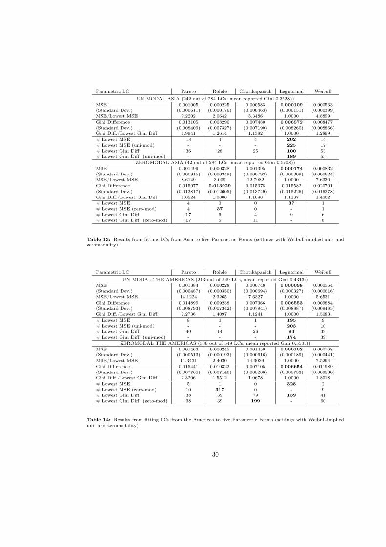
Parametric LC Pareto Rohde Chotikapanich Lognormal Weibull
UNIMODAL ASIA (242 out of 284 LCs, mean reported Gini 0.3628))
MSE 0.001005 0.000225 0.000583 0.000109 0.000533
(Standard Dev.) (0.000611) (0.000176) (0.000463) (0.000151) (0.000399)
MSE/Lowest MSE 9.2202 2.0642 5.3486 1.0000 4.8899
Gini Difference 0.013105 0.008290 0.007480 0.006572 0.008477
(Standard Dev.) (0.008409) (0.007327) (0.007190) (0.008260) (0.008866)
Gini Diff./Lowest Gini Diff. 1.9941 1.2614 1.1382 1.0000 1.2899
# Lowest MSE 18 4 4 202 14
# Lowest MSE (uni-mod) - - - 225 17
# Lowest Gini Diff. 36 28 25 100 53
# Lowest Gini Diff. (uni-mod) - - - 189 53
ZEROMODAL ASIA (42 out of 284 LCs, mean reported Gini 0.5208))
MSE 0.001499 0.000328 0.001395 0.000174 0.000832
(Standard Dev.) (0.000915) (0.000349) (0.000793) (0.000309) (0.000624)
MSE/Lowest MSE 8.6149 3.009 12.7982 1.0000 7.6330
Gini Difference 0.015077 0.013929 0.015378 0.015582 0.020701
(Standard Dev.) (0.012817) (0.012605) (0.013749) (0.015226) (0.016278)
Gini Diff./Lowest Gini Diff. 1.0824 1.0000 1.1040 1.1187 1.4862
# Lowest MSE 4 0 0 37 1
# Lowest MSE (zero-mod) 4 37 0 - 1
# Lowest Gini Diff. 17 6 4 9 6
# Lowest Gini Diff. (zero-mod) 17 6 11 - 8
Table 13: Results from fitting LCs from Asia to five Parametric Forms (settings with Weibull-implied uni- and
zeromodality)
Parametric LC Pareto Rohde Chotikapanich Lognormal Weibull
UNIMODAL THE AMERICAS (213 out of 549 LCs, mean reported Gini 0.4313))
MSE 0.001384 0.000228 0.000748 0.000098 0.000554
(Standard Dev.) (0.000487) (0.000350) (0.000694) (0.000327) (0.000616)
MSE/Lowest MSE 14.1224 2.3265 7.6327 1.0000 5.6531
Gini Difference 0.014899 0.009238 0.007366 0.006553 0.009884
(Standard Dev.) (0.008793) (0.007342) (0.007941) (0.008887) (0.009485)
Gini Diff./Lowest Gini Diff. 2.2736 1.4097 1.1241 1.0000 1.5083
# Lowest MSE 8 0 1 195 9
# Lowest MSE (uni-mod) - - - 203 10
# Lowest Gini Diff. 40 14 26 94 39
# Lowest Gini Diff. (uni-mod) - - - 174 39
ZEROMODAL THE AMERICAS (336 out of 549 LCs, mean reported Gini 0.5501))
MSE 0.001463 0.000245 0.001459 0.000102 0.000768
(Standard Dev.) (0.000513) (0.000193) (0.000616) (0.000189) (0.000441)
MSE/Lowest MSE 14.3431 2.4020 14.3039 1.0000 7.5294
Gini Difference 0.015441 0.010322 0.007105 0.006654 0.011989
(Standard Dev.) (0.007768) (0.007146) (0.008286) (0.008733) (0.009530)
Gini Diff./Lowest Gini Diff. 2.3206 1.5512 1.0678 1.0000 1.8018
# Lowest MSE 5 1 0 328 2
# Lowest MSE (zero-mod) 10 317 0 - 9
# Lowest Gini Diff. 38 39 79 139 41
# Lowest Gini Diff. (zero-mod) 38 39 199 - 60
Table 14: Results from fitting LCs from the Americas to five Parametric Forms (settings with Weibull-implied
uni- and zeromodality)
30