Course: 390026 (Economic Literature Seminar: Risk, Income Inequality, and Information Structures)

Instructor: Prof. Manfred Nermuth

Submitted by: Amjad Naveed (a1047825)

Application of Lorenz Curves in Economics

By

N. C. Kakwani

Focus of the paper:

The main focus of the paper is to extend the concept of the Lorenz curve and generalized it to study

the relationships among the distributions of different economic variables1. The extended version of

Lorenz curve is called concentration curves, and the Lorenz curve is only a special case of

concentration curves.

What is Lorenz Curve?

In economics, the Lorenz curve is a graphical representation of the cumulative distribution function

of the empirical probability distribution of wealth. It is often used to represent income distribution,

where it shows for the bottom percentage (x %) of households, what percentage (y %) of the total

income they have. Lorenz curve is drawn in the following figure 1, where percentage of households is

plotted on the x-axis and the percentage of income on the y-axis.

Figure 1

The Gini coefficient is usually used to measure the income inequality and that is based on

Lorenz curve (figure 1). The line at 45 degrees represents perfect equality of incomes. The 1 The interest in the Lorenz curve technique has been revived by Atkinson (1970) who provided a theorem relating the social welfare function and the Lorenz curve.

Gini coefficient can then be thought of as the ratio of the area that lies between the line of

equality and the Lorenz curve (marked 'A' in the figure 1) over the total area under the line of

equality (marked 'A' and 'B' in the diagram); i.e., G=A/(A+B).

Since, A+B=0.5, the Gini index, G=A/0.5=1-2B. If the Lorenz curve is represented by the

function Y = L(X), the value of B can be found with integration and:

.211

0dXXLG

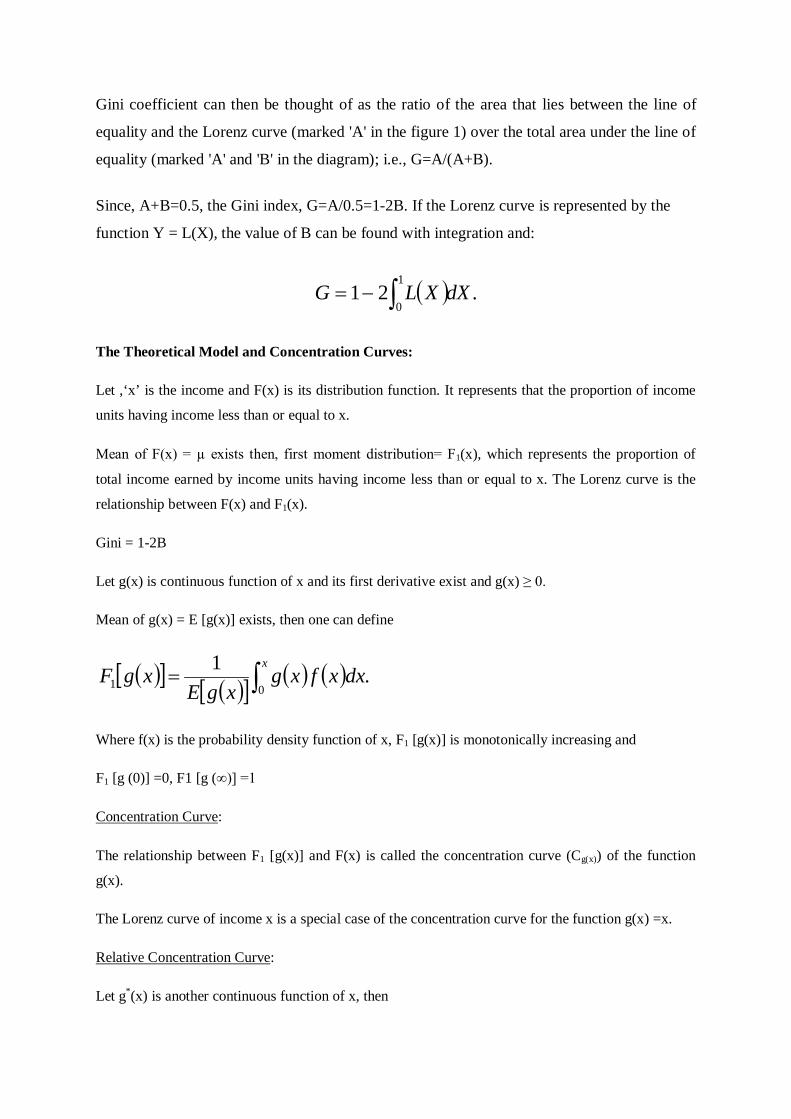
The Theoretical Model and Concentration Curves:

Let ,‘x’ is the income and F(x) is its distribution function. It represents that the proportion of income

units having income less than or equal to x.

Mean of F(x) = µ exists then, first moment distribution= F1(x), which represents the proportion of

total income earned by income units having income less than or equal to x. The Lorenz curve is the

relationship between F(x) and F1(x).

Gini = 1-2B

Let g(x) is continuous function of x and its first derivative exist and g(x) ≥ 0.

Mean of g(x) = E [g(x)] exists, then one can define

x

dxxfxgxgE

xgF01 .1

Where f(x) is the probability density function of x, F1 [g(x)] is monotonically increasing and

F1 [g (0)] =0, F1 [g (∞)] =1

Concentration Curve:

The relationship between F1 [g(x)] and F(x) is called the concentration curve (Cg(x)) of the function

g(x).

The Lorenz curve of income x is a special case of the concentration curve for the function g(x) =x.

Relative Concentration Curve:

Let g*(x) is another continuous function of x, then

x

dxxfxgxgE

xgF0

**

*1 .1

The graph of F1 [g (x)] versus F1 [g*(x)] will be called the relative concentration curve of g(x).

On the basis of above function, following theorem holds.

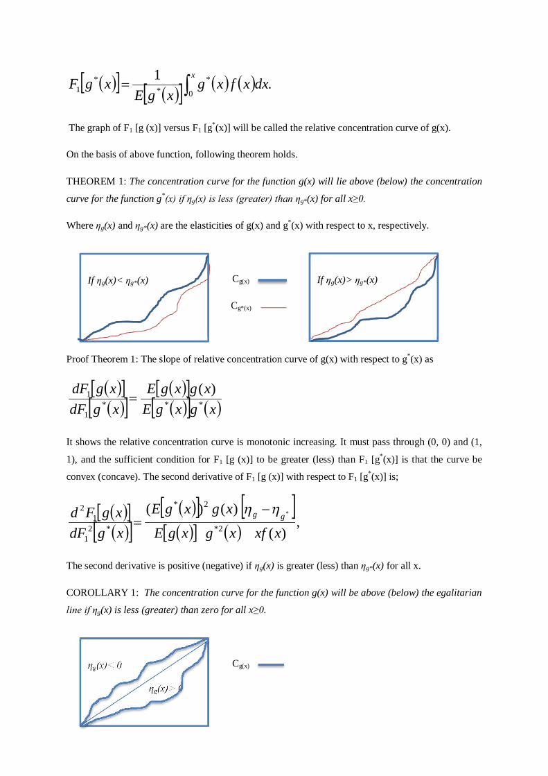
THEOREM 1: The concentration curve for the function g(x) will lie above (below) the concentration

curve for the function g*(x) if ηg(x) is less (greater) than ηg*(x) for all x≥0.

Where ηg(x) and ηg*(x) are the elasticities of g(x) and g*(x) with respect to x, respectively.

Cg(x)

Cg*(x)

Proof Theorem 1: The slope of relative concentration curve of g(x) with respect to g*(x) as

xgxgE

xgxgExgdFxgdF

***1

1 )(

It shows the relative concentration curve is monotonic increasing. It must pass through (0, 0) and (1,

1), and the sufficient condition for F1 [g (x)] to be greater (less) than F1 [g*(x)] is that the curve be

convex (concave). The second derivative of F1 [g (x)] with respect to F1 [g*(x)] is;

,

)(

)()(2*

2*

*21

12

*

xxfxgxgE

xgxgE

xgdFxgFd gg

The second derivative is positive (negative) if ηg(x) is greater (less) than ηg*(x) for all x.

COROLLARY 1: The concentration curve for the function g(x) will be above (below) the egalitarian

line if ηg(x) is less (greater) than zero for all x≥0.

Cg(x)

If ηg(x)< ηg*(x)

If ηg(x)> ηg*(x)

ηg(x)< 0

ηg(x)> 0

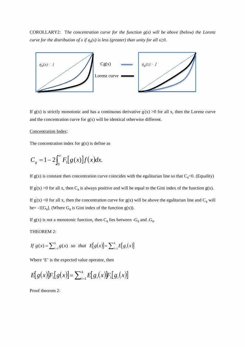
COROLLARY2: The concentration curve for the function g(x) will be above (below) the Lorenz

curve for the distribution of x if ηg(x) is less (greater) than unity for all x≥0.

Cg(x)

Lorenz curve

If g(x) is strictly monotonic and has a continuous derivative g'(x) >0 for all x, then the Lorenz curve

and the concentration curve for g(x) will be identical otherwise different.

Concentration Index:

The concentration index for g(x) is define as

0 1 .)(21 dxxfxgFCg

If g(x) is constant then concentration curve coincides with the egalitarian line so that Cg=0. (Equality)

If g'(x) >0 for all x, then Cg is always positive and will be equal to the Gini index of the function g(x).

If g'(x) <0 for all x, then the concentration curve for g(x) will be above the egalitarian line and Cg will

be= -1[Gg]. (Where Gg is Gini index of the function g(x)).

If g(x) is not a monotonic function, then Cg lies between -Gg and +Gg.

THEOREM 2:

k

i ik

ixgExgEthatsoxgxgIf

11)()(

Where ‘E’ is the expected value operator, then

xgFxgExgFxgE ik

i i 111

Proof theorem 2:

ηg(x)< 1

ηg(x)> 1

x

ik

ii

i

x

ik

i

dxxfxgxgE

xgF

anddxxfxgxgE

xgF

011

011

.1

.1

COROLLARY 3: if g(x) =∑k i=1 gi(x) and Cg and Cgi are concentration indices of g(x) and gi(x),

respectively, then

.1 gi

k

i ig CxgECxgE

It is noted that the Theorem 2 and Corollary 3 do not require the functions g(x) and gi(x) to be

monotonic. If we assume that g(x) is a non-decreasing function of ‘x’, then Cg = Gg.

If gi(x) is any function of ‘x’ (not necessarily monotonic), then Cg ≤ Ggi, where Ggi is the Gini index of

gi(x). And from Corollary 3 we have

.1 gi

k

i ig GxgEGxgE

If all gi(x) are non-decreasing functions of ‘x’ then the Gini index of g(x) will be equal to the

weighted average of the Gini indices of individual gi(x).

Applications of the Theorem

The Engel Curve:

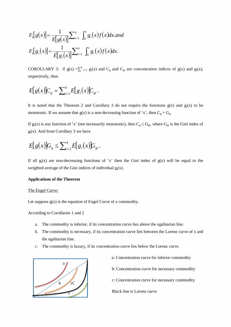
Let suppose g(x) is the equation of Engel Curve of a commodity.

According to Corollaries 1 and 2

a. The commodity is inferior, if its concentration curve lies above the egalitarian line.

b. The commodity is necessary, if its concentration curve lies between the Lorenz curve of x and

the egalitarian line.

c. The commodity is luxury, if its concentration curve lies below the Lorenz curve.

a: Concentration curve for inferior commodity

b: Concentration curve for necessary commodity

c: Concentration curve for necessary commodity

Black line is Lorenz curve

a

b LC

c

Consumption and Saving Functions:

C=f(Y) Consumption is related to income.

If APC (C/Y) decreases as income rises, then income elasticity of consumption will be less than one

and the income elasticity of saving will be greater than one. If both consumption and saving are non-

decreasing functions of income, then it follows from Corollary 2 that the inequality of income is

greater than that of consumption and less than that of saving.

Effect of Direct Taxes on the Income Distribution:

Disposable income is

d1(x) =x-T1(x)

Where ‘x’ is pre-tax income and ‘T1(x) is the tax function.

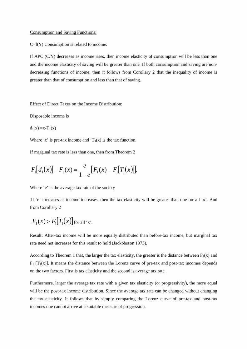
If marginal tax rate is less than one, then from Theorem 2

,)(1

)( 111111 xTFxFe

exFxdF

Where ‘e’ is the average tax rate of the society

If ‘e’ increases as income increases, then the tax elasticity will be greater than one for all ‘x’. And

from Corollary 2

xTFxF 111 )( for all ‘x’.

Result: After-tax income will be more equally distributed than before-tax income, but marginal tax

rate need not increases for this result to hold (Jackobsson 1973).

According to Theorem 1 that, the larger the tax elasticity, the greater is the distance between F1(x) and

F1 [T1(x)]. It means the distance between the Lorenz curve of pre-tax and post-tax incomes depends

on the two factors. First is tax elasticity and the second is average tax rate.

Furthermore, larger the average tax rate with a given tax elasticity (or progressivity), the more equal

will be the post-tax income distribution. Since the average tax rate can be changed without changing

the tax elasticity. It follows that by simply comparing the Lorenz curve of pre-tax and post-tax

incomes one cannot arrive at a suitable measure of progression.

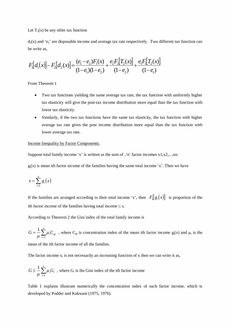
Let T2(x) be any other tax function

d2(x) and ‘e2’ are disposable income and average tax rate respectively. Two different tax function can

be write as,

)1()(

)1()(

)1)(1()()()(

1

211

2

222

21

1212211 e

xTFee

xTFeeexFeexdFxdF

From Theorem 1

Two tax functions yielding the same average tax rate, the tax function with uniformly higher

tax elasticity will give the post-tax income distribution more equal than the tax function with

lower tax elasticity.

Similarly, if the two tax functions have the same tax elasticity, the tax function with higher

average tax rate gives the post income distribution more equal than the tax function with

lower average tax rate.

Income Inequality by Factor Components:

Suppose total family income ‘x’ is written as the sum of ‚‘n’ factor incomes x1,x2,...,xn.

gi(x) is mean ith factor income of the families having the same total income ‘x’. Then we have

n

ii xgx

1

If the families are arranged according to their total income ‘x’, then xgF i1 is proportion of the

ith factor income of the families having total income ≤ x.

According to Theorem 2 the Gini index of the total family income is

n

igiiCG

1

1

, where Cgi is concentration index of the mean ith factor income gi(x) and µi is the

mean of the ith factor income of all the families.

The factor income xi is not necessarily an increasing function of x then we can write it as,

n

iiiGG

1

1

, where Gi is the Gini index of the ith factor income

Table 1 explains illustrate numerically the concentration index of each factor income, which is

developed by Podder and Kakwani (1975, 1976).

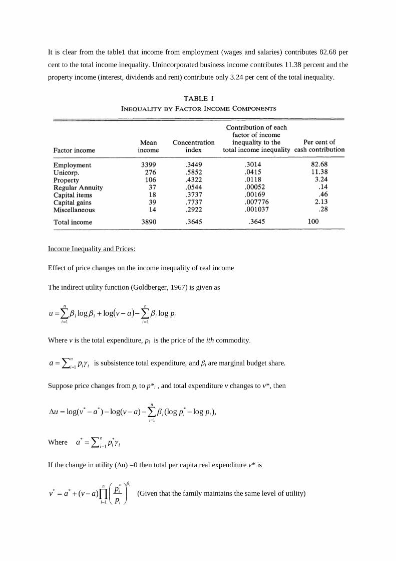
It is clear from the table1 that income from employment (wages and salaries) contributes 82.68 per

cent to the total income inequality. Unincorporated business income contributes 11.38 percent and the

property income (interest, dividends and rent) contribute only 3.24 per cent of the total inequality.

Income Inequality and Prices:

Effect of price changes on the income inequality of real income

The indirect utility function (Goldberger, 1967) is given as

n

i

n

iiiii pavu

1 1logloglog

Where v is the total expenditure, pi is the price of the ith commodity.

n

i iipa1

is subsistence total expenditure, and βi are marginal budget share.

Suppose price changes from pi to p*i , and total expenditure v changes to v*, then

,)log(log)log()log(1

***

n

iiii ppavavu

Where

n

i iipa1

**

If the change in utility (∆u) =0 then total per capita real expenditure v* is

n

i i

ii

ppavav

1

*** )(

(Given that the family maintains the same level of utility)

Let G* be the Gini index of real expenditure, µ is the mean of the money expenditure in the base year,

then according to Theorem 2,

i

i

n

i i

i

n

i i

i

ppaa

Gpp

G

1

**

1

*

*

)(

From the above equation if all prices change in the same proportion, then income inequality is

unaffected.

Let the ratio, v*/v = Index for true cost of living, which converts the money expenditure into real

expenditure.

The ratio G*/G = Index of income inequality that take into account the effect of relative price changes.

It converts the inequality of the money household expenditure distribution to the inequality of the real

household expenditure.

If (G*/G) < 1: Relative price changes are making the expenditure distribution more unequal.

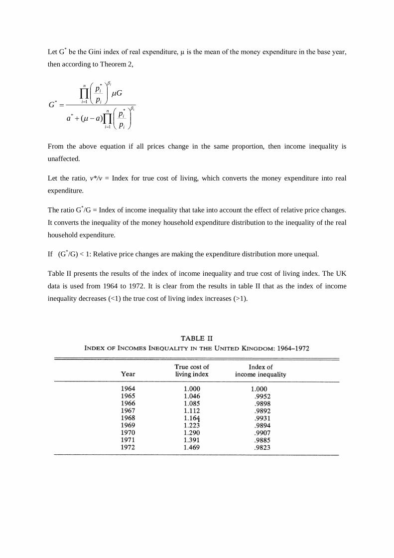
Table II presents the results of the index of income inequality and true cost of living index. The UK

data is used from 1964 to 1972. It is clear from the results in table II that as the index of income

inequality decreases (<1) the true cost of living index increases (>1).