Embed Size (px)
Citation preview

Parametric Model for
Structural Stability
Computation of Chassis
in Tipper Trailers
Maria Lagergren
Degree project in
Solid Mechanics
Second level, 30.0 HEC
Stockholm, Sweden 2011

Parametriserad modell för beräkning av stabilitet hos
tipptrailer-chassin
Maria Lagergren
Examensarbete i Hållfasthetslära
Avancerad nivå, 30 hp
Stockholm, Sverige 2011
Sammanfattning
När en tipptrailer tömmer sin last kan ett vridande moment uppstå om trailern står på lutande
underlag. För att förhindra att lastbilen välter måste vridstyvheten hos chassit vara tillräckligt
hög. Styvheten beror framförallt på hur chassit är dimensionerat. Vid analys av olika
chassigeometrier är modelleringen mycket tidskrävande.
I den första delen av projektet undersöktes vilken elementtyp som ska användas för den här
typen av analyser. För den andra delen av projektet var det nödvändigt att förenkla modellen
så mycket som möjligt. En elementverifierng utfördes, det undersöktes om det är tillräckligt
att använda balkelement istället för skalelement när chassits vridstyvhet ska bestämmas.
Slutsatsen som drogs var att resultant beam elements ska användas för den här typen av
analys.
I den andra delen av rapporten utvecklades ett program som automatiserar genereringen av en
finita element (FE)-modell av ett chassi. Beroende på olika parametrar givna av användaren
skapas en FE-modell av den önskade geometrin. FE-modellen definieras i form av en textfil
som kan läsas in och granskas i en LS-DYNA kompatibel pre-processor.

Parametric Model for Structural Stability Computation
of Chassis in Tipper Trailers
Maria Lagergren
Degree project in Solid Mechanics
Second level, 30 hp
Stockholm, Sweden 2011
Abstract
When a tipper trailer empties the load it carries, a torque occurs if the trailer stands on uneven
ground. To withstand this torque, and prevent the trailer to roll over, the chassis‟ torsional
stiffness must be high enough. The stiffness is highly dependent of the geometry of the
chassis structure. When analysing different geometries the pre-processing of the finite
element (FE)-model is time consuming.
The first part in this master thesis was to assess what element type to use for this type of load
case. It was necessary to simplify the FE-model as much as possible for the second part of the
thesis. A comparison of modelling the chassis with beam elements instead of shell elements
was performed. It was concluded that resultant beam elements should be used when analysing
the torsional stiffness of the chassis.
In the second part of this master thesis a program was developed to automate the FE-
modelling of the chassis, this to be able to compare several chassis structures in a short
amount of time. The program generates a FE-model of the desired chassis structure depending
on parameters given from the user. The program produces a text file, containing information
about the FE-model, which can be read and viewed in a LS-DYNA compatible pre-processor.
FOREWORD
This master thesis was performed in collaboration with SSAB in Borlänge and Epsilon UC
Mälardalen in Solna. Visits to Borlänge were made but the main part of the thesis was carried
out at Epsilon in Solna, during the late spring and summer of 2011.
Many thanks to all my supervisors; Linda Petersson at SSAB for providing me with
knowledge and insight on the subject, Zuheir Barsoum at KTH for support and good
feedback, especially with the writing of the thesis and last but not least Malin Lundgren at
Epsilon for encouragement and support concerning the main part of the thesis.
I also wish to thank Erik Svensson for never ending encouragement and support with the part
of the thesis involving programming.

TABLE OF CONTENTS
1 INTRODUCTION ................................................................................................. 1
1.1 Background .............................................................................................................................. 1
1.2 Purpose ................................................................................................................................... 1
1.3 Delimitations ............................................................................................................................ 2
2 FRAME OF REFERENCE ................................................................................... 3
2.1 SSAB ....................................................................................................................................... 3
2.2 Previous Project Performed at SSAB ...................................................................................... 3
2.3 Finite Element Methods ........................................................................................................... 3
2.4 Torsion Theories ...................................................................................................................... 6
2.5 High Strength Steel ................................................................................................................. 6
2.6 Torque Developed from Standing on Uneven Ground ............................................................ 7
2.7 Determination of Angle of Twist ............................................................................................... 8
3 TEST DESCRIPTION ........................................................................................ 10
3.1 Investigation ........................................................................................................................... 10
3.2 Verification ............................................................................................................................. 10
4 RESULTS .......................................................................................................... 20
4.1 Verification ............................................................................................................................. 20
5 PROGRAM DEVELOPMENT ............................................................................ 23
5.1 Introduction ............................................................................................................................ 23
5.2 Program Language ................................................................................................................ 23
5.3 Aim ......................................................................................................................................... 23
5.4 Structure ................................................................................................................................ 24
6 DISCUSSION .................................................................................................... 28
6.1 Elementary Case 1 ................................................................................................................ 28
6.2 Elementary Case 2 ................................................................................................................ 28
6.3 Framework Models ................................................................................................................ 28
6.4 Conclusions ........................................................................................................................... 29
7 RECOMMENDATIONS AND FUTURE WORK ................................................. 30
7.1 Recommendations ................................................................................................................. 30
7.2 Future Work ........................................................................................................................... 31
8 REFERENCES .................................................................................................. 33
9 APPENDIX ........................................................................................................ 34

1
1 INTRODUCTION
This chapter describes the background of the thesis. The purpose of i t is shortly
described as well as the outlines for the project.
1.1 Background
SSAB, Swedish Steel AB, provides support to clients that develop products with high strength
steel. The support includes advice on product design to optimise the qualities of high strength
steel. A previous project [1] investigated the stiffness of a tipper trailer‟s chassis when
changing the material from conventional steel to high strength steel. In order to give advice on
a certain geometry, seven different finite element models of the tipper trailers framework
were developed. The different models had variations in dimension of the beam‟s cross
sections as well as types of cross sections. Lower weight with satisfying stiffness against an
applied torque was required.
When designing the framework of tipper trailers, experience [2] has shown that a design load
case is when the framework‟s torsional stiffness, that is the relation between an applied torque
and the rotation of the same section, is tested. If the stiffness is not satisfying, the trailer, when
standing on slightly uneven ground, will in worst case roll over while emptying the load it
carries. Figure 1 pictures a tipper trailer from behind, a trailer in an up-lifted position is also
shown.
Hence, in the report [1] the load case tested on the models was an applied torque at the end of
the framework. Due to time and cost limitations only a couple of models were developed and
compared. If there had been a faster way to model the frameworks, a larger investigation on
how the torsional stiffness of the framework changes with varying beam geometry could have
been done.
1.2 Purpose
The main purpose of this thesis was to develop a program that easily generates a finite
element model of a tipper trailer‟s framework. With this tool several different geometries can
be modelled and investigated rapidly. The tool will help the engineer to make a decision on
which geometry to proceed with and recommend to clients. The load case that would be
investigated was stiffness against applied torque. The torque will be applied at the rear of the
framework while a fixed boundary condition is applied at the position of the king pin to hold
the structure in place. The angles of twist of the framework that arises are then compared.

2
1.3 Delimitations
When evaluating the framework models, the angle of twist of the frameworks will be
compared. The stresses have in this case not been of interest. It is assumed that the applied
torque will be small enough to only result in small displacements [1] and that the material will
not deform plastically. Hence, the material used is pure linear elastic and no plastic
deformation is considered.
The generated model would have to be compatible with the FE-solver LS-DYNA. This was
required since SSAB would be using this solver.
Figure 1. The trailer below is a tipper trailer, the trailer above is picturing, to the right, a tipper
trailer emptying the load.

3
2 FRAME OF REFERENCE
This section handles the theory that concerns the thesis.
2.1 SSAB
SSAB is a leading manufacturer of high strength and quenched steel, with global operations.
SSAB‟s strategy is not only to produce specialised steel but also to assist their clients in the
development and design of new products. SSAB‟s products and solutions are used in several
industry sectors; the automotive industry, mining and construction equipment, crane
manufacturers, manufacturers of contracting plant, the recycling industry and the energy
sector [3].
2.2 Previous Project Performed at SSAB
On SSAB‟s account a project had been made where a number of different chassis structures
were compared. The stiffness‟s of the structures were compared through the angle of twist
under an increasing applied moment. At least seven different FE-models were analysed where
small differences in geometric properties were made. The models were modelled with shell
elements and LS-DYNA was used for the implicit analysis. The project showed that a change
to Domex 700, a high strength steel, from conventional steel, lowered the weight of the
chassis while increasing the stiffness. A preferred model could be found where the models
weight also was a decision factor. Material from this project was received from SSAB.
2.3 Finite Element Methods
The Finite Element Method (FEM) is a numerical method that finds approximate solutions to
partial differential equations that are difficult or impossible to solve analytically. The problem
domain is discretised into smaller elements [4].
The problem domain is divided into smaller elements that are connected with nodes. In
general it can be said that the finer the element net (the mesh) is, the more accurate the results
get. Depending on the problem type, different types of elements can be chosen. If the element
choice is considered, time can be saved in the simulation process. For example; a beam should
be modelled with beam elements but can also be modelled with shell or solid elements.
However it is more cost-effective to use a 1D-element than a 3D-element if possible.

4
2.3.1 Beam Elements
A beam element is a two noded 1D-element. There are different types of beams elements,
which are well described in [4]. A planar beam element has two degree of freedoms (DOFs) at
each node, displacement degree in the transverse y-direction and a rotational degree around
the z-axis to describe bending moments. The coordinate system of a beam element is
illustrated in Figure 2. If however the problem domain consists of more than one beam
element with different orientations, a frame or framework is referred. To describe this
situation there are frame elements. They can carry both axial and transverse forces as well as
moments. They combine the properties of truss and beam elements. In most FE-analyse
programs the frame elements are called beam elements. There are two types of frame
elements, planar frames and space frames. The planar frames have a total of six DOFs. Except
the four DOFs that the beam element has it also has the truss‟s DOFs, deflection in the x-
direction. The space frame is a further improved element type. Translational displacements
and rotations in x, y and z-direction in each node makes a total of twelve DOFs. Unlike
trusses beams and frames can transmit forces and moments trough the nodes. In this thesis,
when speaking of beam elements we are referring to space frame elements.
Figure 2. Illustration of a beam‟s coordinate system.
2.3.2 Shell Elements
In a similar manor as for beam elements there are several different shell elements, also
described in [4]. Elements that handle membrane and in-plane effects are called 2D solid
elements. The membrane effects come from loading in the same plane as the element. At each
node there are two degrees of freedom for deflections u and v in x- and y-direction. Plate
elements handle bending or off-plane effects. The loading is applied in a transverse direction
from the plane of the element. In each node this element has three DOFs. One for deflections
perpendicular to the plane, w in z-direction and two degrees of freedom that handles rotations
θx and θy around the x- and y-axis. Both these elements are assumed to have a constant
thickness. If the thickness is varying it is recommended to model this with smaller elements
with different but constant thicknesses. For beam elements, combining the properties of truss
and beam elements we will have frame elements. In two dimensions, combining 2D solid
elements with plate elements we get shell elements. These elements have a total of six degrees
of freedom at each node. Three deflections and three rotational degrees, just as the frame
elements have.

5
2.3.3 Simulation
The simulations were performed in LS-DYNA [5]. LS-DYNA is a commercial finite element
software package. It is command line driven which means that you only need a text editor to
create your input files (ASCII format).
However, there are numerous graphical pre-processing softwares that interpret the models to
compatible input files and in this thesis mainly the commercial software Hypermesh 10.0 [6]
was used. Hypermesh is a pre-processor that is one of the several CAE programs that are
included in Altair Hyperworks. Another pre-processor program used was LS-PrePost [7]
which is LS-DYNAs own pre- and postprocessor program that is freely distributed. It was
used in particular for model checking. Minor modifications in the program were made directly
in a text editor.
When studying the results produced from the solver usually a post-processor is used. In this
thesis both Hyperview and LS-PrePost were utilised for graphical viewing.
2.3.4 Implicit and Explicit Methods
When solving systems that are subjected to transient excitation there are mainly two types of
methods used in solving these, explicit and implicit methods. Explicit methods are used when
the excitation is high or when dynamic effects are of interest, car crashes for example. The
time step is constant and is set sufficiently small enough to keep the solution stable. If
however the excitation is low a small time step will make the solution unnecessary long. The
implicit method is then recommended. In the implicit method a time step is taken and matrix
system equations are solved [4].
2.3.5 LS-DYNA
As earlier mentioned, LS-DYNA is command line driven. This means that an input file to LS-
DYNA is a text file in ASCII format, called a keyword-file. The keywords are for example
*NODE and *ELEMENT, examples of keywords are found to the left in Figure 3. Under each
keyword similar functions are collected [8]. A keyword usually has options for the user to
specify. Options for *ELEMENT, are among others, BEAM, SHELL or SOLID. In Figure 3
the organisation of keywords in LS-DYNA is illustrated. The arrows show the connections
between different keywords. The elements are connected to nodes and parts. The parts then
connect the elements to a material and a cross section.

6
Figure 3. Organisation of keywords in LS-DYNA [9].
2.4 Torsion Theories
Depending on boundary conditions and properties of the cross sections of the beams different
torsion theories must be considered [10]. Two different torsion theories handle two different
types of stress states in the beam. Saint Venant torsion theory implies that for a beam loaded
in torsion, each cross section, throughout the length of the beam, will twist as a rigid body;
there will be no change of the cross section‟s form. However, the cross sections are free to
warp. Warping implies that the cross section gets a deflection in x-direction. A cross section
that is circular will not experience warping. If the cross section is something else but circular
the beam will warp. If warping is restrained, normal and shear stresses will arise. To study
these stresses the Vlasov theory must be applied. The theory combines the shear stresses
according to St Venant and the shear and normal stresses that arise when warping is
prevented. The SSAB Sheet Steel Handbook [10] describes well what to keep in mind when
designing beams subjected to torsion. Generally speaking; if a beam has a thin open cross
section and some sort of boundary conditions applied to it, warping will be restrained and
Vlasov theory must be considered.
In our case the framework has several open cross section beams that will be restrained to
warping. To model these effects, beam elements with warping as a degree of freedom should
preferably be used.
2.5 High Strength Steel
High strength steel has higher yield strength than conventional steel. That is, it can take a
higher load before it starts to deform plastically, although with the same elastic material
properties as conventional steels. Generally, steel with a yield strength above 460 MPa can be
considered as high strength steel [2].

7
Since the high strength steel deforms at higher yield strength, thinner structures can be used.
Thinner structures equal lower weight which for trailers means an increase in payload and in
the long run fewer transports. When designing with high strength steel there are certain design
criteria that must be taken into consideration. In SSAB‟s Sheet Steel Handbook [10] several
recommendations are outlined.
2.6 Torque Developed from Standing on Uneven Ground
If a trailer is emptying the load while standing on uneven ground a moment will act on the
chassis-structure. If the load‟s weight is approximated with a mass point force from the centre
of the trailer we will have the situation showed to the left in Figure 4. The force that makes
the moment to arise can be found as follows. If the trailer is viewed from the side while the
loading is raised with an angle α, we get;
Where the definition of Fx and Fy can be found in Figure 4 and m is the weight of the load and
g the gravitational constant. If the ground has a slope of an angle β there will be resultant
forces in the z-direction. To the right in Figure 4 we see the trailer from behind. We then get
The torque is then calculated as follows
This says that if β is zero the moment will not arise, which is expected if the ground is even.

8
Figure 4. The illustration to the left shows the trailer from the side where the lorry is in an up-
lifted position. The illustration to the right shows the trailer from behind in an up-lifted
position while standing on uneven ground.
2.7 Determination of Angle of Twist
The angle between two vectors, and , can be determined with the scalar product of two
vectors;
(1)
In Figure 5 we see the situation that will be occurring when we apply the torque to the
framework. Using the coordinates from Figure 5 in Equation (1) we get the following.
However, from the analyse we will get resulting deformations for the two points. The
coordinates of the starting points must be considered, we will have
and the same for the other point, where δ is the deformation obtained from the analyse results
and and are the points coordinates at the undeformed state.

9
Figure 5. Illustration of the two points subjected to loads at the rear of the framework. The
coloured red dots symbolise the undeformed state and the red circles are after
deformation.
10
3 TEST DESCRIPTION
This section describes how and why different FE-analyses were performed.
3.1 Investigation
Previous framework-models [1] had been modelled with shell elements. To make a program
which assembly‟s nodes for all these shell elements would probably take longer time than was
set for this thesis. It was therefore decided that a verification test should be done to clarify if
the framework could be modelled satisfactory with beam elements instead of shell elements.
3.2 Verification
Tests were performed to evaluate the different beam elements in LS-DYNA. Tests were also
executed to compare a framework modelled with shell elements to one modelled with beam
elements. It was decided that the angle of twist of the rear of the frameworks at an applied
torque would be compared between the different models.
3.2.1 Beam Element Test
LS-DYNA has a number of different types of beam elements, of which two have been used in
this thesis. They are called cross section integrated (ELFORM=1) and resultant beam
(ELFORM=2) elements [8].
The cross section integrated beam (Hughes-Liu beam) uses through-the-cross-section
integration. The number of integration points over the cross section can be controlled and
hence the accuracy when it comes to the cross section is higher than for the resultant beam.
The resultant beam element (Belytschko beam) uses a „co-rotational technique‟ in the element
formulation to handle large rotations [11]. A disadvantage with the resultant beam element is
that stresses in the beams cannot be handled.
A test comparing the convergence of these elements under a bending test was performed. This
was done by simply adding the number of elements along the length of the beam while
applying the same load case.

11
Figure 6. Elementary case studied to evaluate the different LS-DYNA beam elements.
The case studied consisted of a cantilever beam with a c-cross section with a fixed support at
one end and a load applied to the other end, see Figure 6. In Table 3.1 the dimensions of the
beams length and cross section and the applied force are stated. The displacement in z-
direction at the load point was then collected for an increasing number of elements along the
beam length. These small models were all created by scripting directly in a text editor.
Table 3.1. A table showing the dimensions of the beam and value of applied load.
Dimensions Values Units
F 100 N
l 1 m
h 200 mm
w 80 mm
s 6 mm
t 11 mm
3.2.1.1 Element Types
The two beam elements used were defined with ELFORM = 1 (cross section integration) and
ELFORM = 2 (resultant) under *SECTION_BEAM. For the integrated element type an
integration rule was created with *INTEGRATION_BEAM to be able to define the c-cross
sections dimensions fairly easily. The K parameter, called integration refinement parameter
[8], was put equal to two. This parameter defines how many integration points that should be
used over the cross section. It was put to two, a total of 21 integration points. We wanted to

12
make sure that the element comparison would not be dependent of a choice of low number of
integration points. Other parameters were set to default values. The resultant beam elements‟
cross section were defined under *SECTION_BEAM.
3.2.1.2 Material Model
A linear elastic material model was used. This material model was implemented with
*MAT_ELASTIC. The material parameters are; Young‟s modulus 210 GPa, Poisson‟s ratio
0.3 and a material density of ton/mm3.
This material model and its material parameters will be used for all simulations performed in
this thesis.
3.2.1.3 Load and Boundary Conditions
A load F = 100 N was applied, in z-direction, with *LOAD_NODE to the end node. At the
other end all six degrees of freedom are fixed with *BOUNDARY_SPC_NODE.
This load and boundary condition will also be used in section 3.2.3.
3.2.1.4 Simulation
An implicit solution was performed on the load case with LS-DYNA [5]. Default settings
were chosen and the automatic step size control, under *CONTRL_IMPLICIT_AUTO [12],
was active.
This solver was used for all simulations performed throughout this thesis.
3.2.2 Warped Beam Element Test
To study the effects of modelling with beam elements with a warping degree of freedom the
same test as described in 3.2.1 was performed with warped beam elements. This model should
experience warping since the beam has an open cross section and fixed supports at the end.
The cross section‟s dimensions are again stated in Table 3.1. This model was also created by
scripting in a text editor. The few modifications made to the previous model are described in
the following two subsections. In the third subsection a description of a reference case model
is described.
3.2.2.1 Element Type
The elements are implemented with the *ELEMENT_BEAM_WARPAGE option and
ELFORM=11 under *SECTION_BEAM. The warpage beam elements demands extra scalar
nodes that are created with *NODE_SCALAR. Between two beam elements only one scalar
node is needed. Again an integration rule was defined, as in 3.2.1.1, to simplify the
implementation of the cross section‟s dimensions. Numbers of elements tested along the
length of the beam were two, four and eight.

13
3.2.2.2 Boundary Condition
The same boundary conditions as in 3.2.1.3 were applied. However, the scalar node at the
fixed end side had its degree of freedom fixed as well.
3.2.2.3 Reference Case
To have results to compare with, the same elementary case was modelled with four noded-
shell elements (ELFORM=1 under *SECTION_SHELL) in Hypermesh 10.0. The elements
had a side length of approximately 30 mm, with a total number of 400 elements and 440
nodes. The load, , was applied to the middle point of the cross section, see Figure
7. At the other end of the beam, fixed boundary conditions were applied to the set of nodes
with *BOUNDARY_SPC_SET. A mean value of the deflection from the nodes on the cross
section where the load was applied was calculated.
The deflections from the warped beam element-model were then compared to the deflection
from the shell model.
Figure 7. Picture showing the mesh of the beam built with shell elements, this to illustrate the
warping effects.
3.2.3 Framework Built with Shell Elements
A FE-model of the tipper trailer‟s framework was built with Hypermesh 10.0. Measurements
were taken from one of the FE-models from the report previously mentioned [1]. Some details
from the previous model were not modelled, only the main features. A comparison of the
structural stability will be performed between this shell element-model and a framework
modelled with beam elements, which will be described in section 3.2.4.

14
3.2.3.1 Geometry
The FE-model was mainly built in Hypermesh 10.0. Some error search was also made in LS-
PrePost [7]. Finally some final touches were made by scripting in a text editor.
Figure 8 shows the reference model together with width and length in mm. The king pin is the
device that connects the chassis to the truck. The area around the king pin is mostly the same
for all chassis-structures. The two longest beams with an I-cross section will be called main
beams and the beams connecting the two (in this case there are five of them) will be referred
to as cross beams. The small reinforcements on the main beams, which are indicated in the
figure, are examples of details that were not modelled in the new FE-model, nor were the
small holes. Simplifications were also made in the area around king pin and at the rear where
a cylinder is positioned to hold the lorry. The differences can be seen by comparing the front
and rear of the chassis in Figure 8 and Figure 9.
The cross beam closest to the king pin area has a c-cross section, the three following cross
beams have box-shaped cross sections and the cross beam furthest to the rear has an
approximated c-cross section.
For clarification of the directions in the model; the x-direction is defined in the same direction
as the length of the beam, the y-direction is defined as the longitudinal transverse direction of
the length of the beam and finally the z-direction is defined as the horizontal transverse
direction of the length of the beam.
3.2.3.2 Elements and Mesh
The FE-model, see Figure 9, was built with four-noded shell elements (ELFORM = 16 under
*SECTION_SHELL) and five trough the thickness integration points. The elements had a
side length of approximately 30 mm. The cross beams are connected to the main beams with
shared nodes. The different colours symbolise different thicknesses of the shell elements.
It was decided through discussions with SSAB that the area around king pin would not have a
great influence on the resulting angle of twist. The area was therefore simplified. The front
(flat in shape) and the back (box-shaped) of the king pin-area, see Figure 9, were constructed
similar to the reference model. A rigid body was then created, connecting the nodes at the
bottom, this is illustrated in Figure 10. The model contained approximately elements
and nodes.

15
Figure 8. A picture showing the geometry of the reference model.
Figure 9. FE-model of the framework modelled with shell elements. Loads and boundary
conditions are also shown.

16
Figure 10. A picture of the FE-shell model from beneath showing the rigid body at the front of the
chassis. For illustration reasons a thicker line has been drawn over the nodes connected
to the rigid body.
3.2.3.3 Boundary Conditions and Loads
A pair of forces of each N was applied at the rear of the chassis in positive and
negative y-direction, to nodes at the middle of the cross section. This generated a moment of
kNm. The loads where applied with the command *LOAD_NODE. The forces were
aligned with the y-axis and at a large angle of twist a reduced torque would have to be
compensated. This was however not done in this case since the loads were not judge to
generate a large rotation.
At the position of the king pin, where a rigid body has been created, fully constrained
boundary conditions have been applied with
*CONSTRAINED_NODAL_RIGID_BODY_SPC and the option to constrain all
displacements and all rotations. This condition applied to all nodes connected to the rigid
body.
The loads and boundary condition will be modelled the same way in the beam model
described in the next section.
3.2.4 Framework Built with Beam Elements
The FE-model was again built in Hypermesh 10.0. The area around the king pin was not
modelled with beam elements but with shell elements. It was taken from the model previous
described. This was a simplification done to save some time modelling and it was discussed to
not be affecting the results.
3.2.4.1 Geometry
All dimensions of the beams‟ cross sections, lengths of main beams and cross beams were
chosen to be as consistent as possible with the model with shell elements.

17
3.2.4.2 Elements and Mesh
The elements in the king pin-area are described in section 3.2.3.2. The beam elements were
created with ELFORM = 2 under *SECTION_BEAM. Depending on position in the
framework the elements were defined with different cross sections. In Figure 11 the FE-model
is shown with the different cross sections of the beam elements pointed out. The cross
sections were defined in *SECTION_BEAM.
At the connection between the main beams and the king pin-area rigid bodies were created.
All nodes at the cross section were connected to the closest beam element, see Figure 12.
Figure 11. FE-model of the framework built with mainly beam elements. Rigid bodies connect the
cross beams to the main beams as well as the area around king pin modelled with shell
elements to the main beams. Loads and boundary conditions are also illustrated.

18
Figure 12. Picture showing the connection point between the shell elements and the beam
elements. A rigid link connects all nodes on the thicker line to the node of the beam.
The line was drawn for illustration.
The main beams have I-cross sections where at the front of the chassis the beams are
increasing in height. This was modelled with smaller beam elements that had constant cross
sections but where the height of the cross section increased for each element, see Figure 13.
Where the main beam has a slight slope there will be elements overlapping each other as well
as some gaps where material is missing. This is inevitable and will hopefully not affect the
results too much.
Three cross sections were defined to model the cross beams. Two c-cross sections and one
box-shaped. Rigid links where used in order to get the positioning of the cross beams similar
to that of the shell model. In Figure 14 it is described how LS-DYNA positions a c-cross
section and a box-shaped cross section relative the node. With this in mind a rigid body was
created between the cross beam‟s node and the closest node on the main beam.
Number of beam elements added up to 120 and number of nodes to 230. In total the model
consisted of 2 800 elements and 3 000 nodes.

19
Figure 13. Picture showing the area of the frame work where the I-cross sections have varying
heights.
Figure 14. C-cross section and box-shaped cross section positioned relative the node, here marked
red. The node is positioned at half the width and half the height of the cross section.
3.2.5 Warped Beam Elements
Another test was performed to study the effect of allowing warping for the beam elements,
now in a larger model. Some of the beam elements in the FE-model previously described
were changed to integrated warped beam elements (ELFORM = 11). The same implement
procedure as described in section 3.2.2 was followed.
Changing the beam elements to warped beam elements could not be performed in Hypermesh.
It was done by editing the keyword file in a text editor. This was time consuming and
therefore not all beam elements were changed. In particular we were expecting warping in the
cross beams and hence, they were changed. The main part of the main beam, where the
elements have the same cross sections, were changed to warped beam elements as well.

20
4 RESULTS
This section handles results gathered from the tests performed in section 3.
4.1 Verification
Tests were performed to compare two different beam elements in LS-DYNA. An elementary
case was studied. Tests were also done to compare differences when modelling with beam
elements instead of shell elements. These tests were performed on a framework structure.
4.1.1 Convergence Test
A cantilever beam, with a c-cross section, subjected to a bending load in z-direction was
modelled with two different types of beam elements. The number of elements was increased
along the length of the beam to study the convergence of the elements. The deflections in the
load point were studied. The handbook formula was used to have an analytical value to
compare the results with. Case 1 in table 32.1 in [13] was studied. The results can be found in
Table 4.1.
Table 4.1. Table showing z-displacements for elementary case modelled with two different types of
beam elements.
Deflections
Number of elements Integrated * [mm] Resultant ** [mm]
2 8.53E-03 9.00E-03
4 8.93E-03 9.00E-03
6 9.01E-03 9.00E-03
8 9.03E-03
12 9.05E-03
Handbook formula [mm]
8.56E-03
* Cross section integrated beam elements (ELFORM = 1)
** Resultant beam elements (ELFORM = 2)

21
4.1.2 Warped Beams Test
A cantilever beam, with a c-cross section, subjected to a bending load in z-direction was
modelled with warped beam elements in one test and shell elements in another. The deflection
in z-direction for each case was then compared. For the beam model, the z-displacement in
the load point was studied. In the shell model a mean value was calculated from the
deflections of the nodes at the cross section were the load was applied. The results can be seen
in Table 4.2.
Table 4.2. Table showing z-displacements for elementary case modelled with warped beam
elements and shell elements.
Deflections
Number of elements Warped beam elements * [mm] First order shell elements [mm]
2 2.88E-02
4 3.64E-02
8 3.91E-02
400
2.16E-02
* Integrated warped beam (ELFORM = 11)
4.1.3 Shell Model
A model of a typical tipper trailer framework was modelled with first order shell elements.
The angle of twist under a torque of 10.1 kNm was calculated. It was assumed that the
displacements along the length of the framework (x-direction) were small and only the
displacements in the other two directions (y- and z-direction), transverse to the length of the
beam, were studied. The nodes‟ displacements in y- and z-direction on the cross section at the
rear of the framework were collected with Hyperview [6]. A mean value was calculated to
symbolise a point value.
) and )
Where Pos_left and Pos_right are the points where the loads are applied and
are the mean values of the deflections in y- and z-direction.
With the deformation for the two main beams an angle could be calculated between the
undeformed and deformed framework, this calculation is described in section 2.7. The
resulting angle of twist for the shell model is defined in Table 4.3. Deformation plots of the
whole framework have been added to the Appendix. The deformation plots show the beam
elements‟ cross sections. The cross sections‟ orientations are defined with a node that is fixed

22
in space. When the framework is deformed the cross sections will not deform correctly, and
the result plots might look slightly off. This is only a viewing error and will not affect the
displacement results.
Also, added to the Appendix, is a result plot showing the von Mises stresses in the shell
model. From this plot it can be verified that the stresses in the model is low.
Table 4.3. Resulting angle of twist at applied torque for framework modelled with shell
elements.
Applied torque [kNm] Angle of twist [°]
10.1 1.78
4.1.4 Beam Model
The framework modelled with mostly beam elements (ELFORM = 2) had a torque applied to
it. The angle of twist was calculated. Another model with warped beam elements was also
analysed for the same type of loading. The deformations in y- and z-direction were collected
from the nodes where the loads were applied, and the angle of twist was calculated. The
procedure was similar to that described in the previous section. The results from these two
cases are defined in Table 4.4.
Table 4.4. Angle of twist of frameworks modelled with beam elements and warped beam elements
under an applied torque of 10.1 kNm. The difference in percent from the shell model
described in section 4.1.3 is also presented.
Angle of twist [°] Difference from shell model [%]
Model 1 (beam elements) 1.703 -4.3
Model 2 (warped beam elements) 1.700 -4.5

23
5 PROGRAM DEVELOPMENT
In this chapter the development of the program is outlined. It describes which
programming language was used, how the program was constructed and
composed.
5.1 Introduction
The tests that were performed gave valuable input on the structure of the program. It was clear
that it would be sufficient to model the framework with beam elements. The program should
create the necessary beam elements and loads and then this model should be connected to the
FE-model already created around the king pin, i.e. do what was done in section 3.2.4 but
much quicker and almost automated.
5.2 Program Language
A programming language had to be chosen. It had to be easy to handle text files for
input/output, handle graphical user interfaces (GUIs), be easy to learn for beginners and,
perhaps most important, be a language which SSAB approved of. The choice came down to
Python [14]. It handles text files easily and it did not seem too hard to create GUI‟s. There are
numerous GUI frameworks compatible with Python. After some research the tool wxPython
[15] was chosen. Almost all knowledge about this program was collected from an online
tutorial [16].
5.3 Aim
The aim of the program was to be able to generate a FE-model of a framework fast. Some
parameters should preferably be variable in the program, and a list of desired parameters was
made following discussions with SSAB. More specifically, the end user should be able to:
Choose the number of cross beams, position them and apply different cross sections
Choose the length of main beams, change cross sections, and decide how the tilting
area, shown in Figure 13, should look like
Change material parameters
Boundary conditions and torque loads should also be possible to apply.

24
5.4 Structure
The program was built very much in the way LS-DYNA organises and structures elements,
material models and nodes, which is described in section 5.
Classes were made for elements, node points, materials, cross sections, parts, rigid bodies and
node lists. In Figure 15 a schematic drawing is shown to illustrate the classes (e.g. Node,
Element and Part) and their instances (NID, EID and PID).
When an object of a class had been created it was stored in a „global‟ vector. When all user
choices had been made in the program and the model was fully specified, a function collected
the objects from the global vectors and wrote information on them and their instances in a text
file for LS-DYNA.
Figure 15. Picture showing the class structure of the program.
5.4.1 Material Implementation
In Figure 15, if the class Material is studied, we see that Material and its instances do not
depend on any other class. The same applies to the class Section. This implies that materials
and different cross sections can be defined, created and stored without regards to other
classes. One might say that this is also the case for the node points, but they should not be
created unless they belong to an element. They will be created when information about the
element (position and orientation) is collected. It was determined that materials should be
created first.
A rather large number of cross sections probably had to be created. In order to avoid
confusion, it was decided to create a few cross sections at a time. The program was divided
into subprograms that handled material, main beams, cross beams and loads, see Figure 16.
The cross sections are designed in the Main Beam and Cross Beam GUIs.

25
Figure 16. Picture showing a scheme over the program layout.
5.4.2 Main Beam Creation
The main beams are created when the materials are defined. The main beams are not
dependent on anything but the position of the connecting nodes at the shell model around the
king pin. These two positions are stored in the background of the program. The left point,
when viewing the framework from above, is set to origo, see Figure 17. When the model is
finished the positions of the nodes will be updated to the same coordinate system as the shell
model. The main beam was divided into five sections, called Parts, in order to facilitate
positioning of its sloping part. The Parts positions were defined through a horizontal length
(x-value) and vertical offset (y-value) from origo according to Figure 17, which illustrates the
left main beam. If a straight main beam is wanted, five positions still have to be defined. For
each Part a number of elements is also decided.
When defining cross sections for the Parts it would be convenient not having to define every
single cross section in the Parts that are tilting. In these areas the cross sections have linearly
increasing heights. It would be sufficient to define the two end cross sections of each Part.
Given the number of elements, a function then defines the cross sections in between. The
function changes the cross section‟s height, as defined in [17]. The other parameters are held
constant. If a Part is not tilting the same cross sections are referred to at both ends. The right
main beam is automatically generated with different coordinates in z-direction. It is taken for
granted that the orientations of the cross sections are the same as in Figure 17.

26
Figure 17. Figure showing the framework from the side. The picture describes how the main beam
is defined by Parts. The second picture illustrates how to define cross sections for a Part
with slope.
5.4.3 Cross Beam Creation
For each cross beam, a number of elements, a cross section with orientation, position along
the main beam and possibly an offset from it had to be defined. To address the positioning of
the cross beam, a length in the x-direction sets its distance from origo. To position it
vertically, a length in the y-direction represents the distance from the line that connects the
Part‟s positioning nodes. This is illustrated in Figure 18 and the lengths are called and .
The red line is a rigid link that is created in order to connect the cross beam‟s node to the
closest node belonging to the main beam.
Next, a cross section has to be defined, which is done in the same way as for the main beam.
To orientate the cross section the user is asked to define a 2D-vector to point in the same
direction as the cross section‟s s-axis. The s-axis definitions for a c-cross section and a box-
shaped cross section are defined in Figure 14. Other cross sections can be found in [17]. For
the case pictured in Figure 18 the vector is . A third node is created in the vector
direction to orientate the beam‟s cross section.
When these steps have been made a cross beam is created. To create another the same steps
have to be repeated. All defined cross sections are stored, to avoid creating the same cross
section twice.

27
Figure 18. Picture of the cross beam‟s positioning alongside the main beam. The line connecting
the position nodes has been drawn for illustration. The line connecting the cross beam‟s
node and the main beam‟s node is a rigid link.
5.4.4 Define Loads
Last to define are the loads. The positions of them are constant, at the framework‟s rear; we
only need to decide the magnitude.

28
6 DISCUSSION
In this section the results from section 4 are discussed. Listed last in the section
are conclusions drawn.
6.1 Elementary Case 1
The first test done was a bending test performed with two different beam elements and
increasing number of elements. We see in Table 4.1 that a stable value was found already at
two elements when using the resultant beam element. The deflection does not change when
the number of elements is increased. For the integrated beam elements the stiffness of the
beam decreases with increasing number of elements. It is hard to tell if the value of the
deflection is stable with twelve elements, perhaps more elements are needed to get a stable
value. The analytical value is in the same region as the numerical ones.
The model would not be as dependent of number of elements if the resultant beam elements
were used. This was the reason to why the elements implemented in the program were the
resultant beam elements.
6.2 Elementary Case 2
In a second test beam elements with warping degree of freedom was studied. Here, to have a
reference case to compare with, the same cantilever beam was modelled with shell elements.
In Table 3.1 we see that the reference value is smaller than the values calculated with the
warped beam elements. We also see that the deformation is increasing when the number of
elements is increased. When we allow warping a decrease in stiffness is expected. A guess
was that the value would not deviate too much from the reference case, modelled with shell
elements, which it unfortunately seems to do. The value from the shell (reference-) model is a
mean value, however the largest of those values were mm. With four beam
elements we see a larger deformation than this top value. It is hard to tell if we will have any
convergence for the warped beam model, and how many elements to use. More simulations
would have to be done to establish this. One possibility is also that the elements are defined
wrongly. Documentations on how to utilise and implement these elements were poor. There
was some help received from the support at the Engineering Research AB, ERAB [18], but
the elements and their implementation was new for them as well.
6.3 Framework Models
In Table 4.4 we see the results from the two different beam models and also the difference in
percent from the shell model. The difference is under five percent which is seen as a good

29
result, especially when comparing the number of elements used in the different models. In the
area where beam elements are used the number of elements were reduced from 20 000 to 100.
We need however to think about that the shell model was a simplified model of a tipper
trailer‟s framework. Had it been more detailed perhaps the results would not have been as
agreeing. If for example stiffeners had been used to stabilise the main beams this would have
been difficult to model in the beam element-model. This would probably yield a higher
difference in angle of twist between the shell and beam-model.
One had hoped that the beam elements with warping had given us a lower stiffness of the
framework. Instead we see almost no difference in angle of twist between the two models.
However from the elementary case studied with warped beam elements we saw that they gave
very unpredictable results. Conclusions should probably not be drawn from the framework
modelled with these elements. It was however positive to see that the „regular‟ beam elements
gave us a stiffness similar to the shell model.
6.4 Conclusions
The conclusions drawn from the discussion are;
When analysing the framework‟s torsional stiffness it is concluded that the use of
resultant beam elements are preferred
It is clear that a larger investigation on the warped beam elements must be performed.
For now, it is not worth the effort of implementing this extra degree of freedom to the
framework analysis
To model the framework with beam elements instead of shell elements is a good
approximation

30
7 RECOMMENDATIONS AND FUTURE WORK
In this section advice will be given on how to utilise the tool. Recommendations
are also given from the conclusions drawn in the previous section. Suggestions
for future work are also stated.
7.1 Recommendations
7.1.1 Beam Elements
The two different beam elements that have been investigated, resultant and integration beam
elements, both have advantages and disadvantages.
Integration Beam Elements
Advantages
Possibility to study the stress state
Possibility to define own integration rules
Compatible with most material models
Disadvantages
Need to define an own integration rule if the cross section is not rectangular
Not compatible with Hyperbeam, a cross section definition program available in
Hypermesh.
Need a finer mesh to get convergence
Resultant Beam Elements
Advantages
Easy to implement, compatible with Hyperbeam
Converge quickly with only a few elements
Disadvantages
Show no stress results
Not compatible with as many material models as integration beam elements

31
The ease of which the resultant beam elements can be implemented and the convergence with
few elements where the two main reasons to why the resultant beam elements where
implemented in the program.
7.1.2 Framework Modelling
From the comparison between the shell model and the beam model we see that the difference
in angle of twist is not very big. However the shell model can be modelled more detailed and
true to original geometry. For example the real frameworks have stiffeners to stabilise the I-
cross section of the main beam. These would be difficult to model in the beam model. In the
shell model the cross beams are connected to the main beams with common nodes. There is
probably a more correct way to model these welds. The more detailed and true to reality the
shell model gets, larger differences between the stiffness of the shell and beam models are
expected.
7.1.3 Program Use
The way to use the program is probably to model a larger number of beam element models
and compare the stiffness of different geometries. From these results, decision can be made on
which geometries to model in detail with shell elements. In the detailed shell-models stresses
can also be analysed.
7.1.4 Warped Beam Elements
In LS-DYNA there are two types of beam elements that allow warping. In this thesis only the
integrated warped beam was implemented. The other type is called resultant warped beam
element. The reason to why these elements were not tested was due to the complicated
implementation. Several parameters concerning the cross section had to be hand calculated. It
would have been too cumbersome to use these in the program. In the end, no warped beam
elements were implemented in the program since the results from them where not satisfying.
7.2 Future Work
There are several topics worth studying in future research. First, a larger investigation on
warped beam elements should be done. We did not see a change in the results from the
framework analysis, when changing to the warped beam elements. From the small elementary
case study on the warped beam elements we saw some unreliable results. This stresses even
more that a larger scale investigation on the warped beam elements should be performed. It
should be mentioned that in the elementary case study, the displacements in the applied load

32
direction was compared. The displacements in the two other directions should in this further
investigation be studied as well.
It would be interesting as well to study the other type of warped beam elements, the resultant
warped beam elements. What could be seen from the test between the beam elements without
warping was that the resultant beam type did converge with fewer numbers of elements than
the integrated beam type did. If this is also the case with the warped beam types we could
perhaps get better results in the test performed in section 3.2.2.
The investigation between the frameworks modelled with beam and shell element can be
extended. It would be interesting to see how the results vary when more details are added to
the shell model. The difference gained of 4.3% will probably increase with a more detailed
shell model.
It would also be interesting to test different boundary conditions and load cases for the
framework. For example, it would be interesting to study the global bending of the framework
which was left out in this thesis.
The largest part of the beam model that is created, is the area around king pin, constructed
with shell elements. Since we have a rigid body connecting the nodes it can be debatable if we
need to use all these shell elements. The result plots in Appendix shows that the area around
king pin experience little deformation. It could perhaps be sufficient to create rigid nodes
between the point of king pin and the nodes attached to the beams.
Improvements in the program could be to let the user implement a different type of beam
element. Currently resultant beam elements are predefined. As an alternative the integration
beam elements could be implemented as well. If the warped beam elements are investigated
properly they too could be implemented in the program. Different load cases than the pre-
defined applied moment could be another further development.
Instead of manually extracting the displacements from Hyperview this step can be automated.
A script can be written to extract the resulting displacements from the current nodes, directly
from the result files and then compute the resulting angle of twist.

33
8 REFERENCES
[1] Anders Jonsson, “Stiffness analyses of trailer frames”, Engineering Research no.
10002-27, 2010
[2] Linda Petersson SSAB Centre of Excellence Structural Technology,
[email protected], oral reference
[3] SSAB webpage, http://www.ssab.com/en/, Sept 13th
2011
[4] G. R. Liu & S.S. Quek, “Finite Element Method: A Practical Course”,
Butterworth-Heinmann, published 2003, ISBN 0 7506 5866 5
[5] LS-DYNA version mpp971d R5.1.1, http://www.dynamore.se/, Sept 13th
2011
[6] Altair Hyperworks, http://www.altairhyperworks.com/, Sept 13th
2011
[7] LS-PrePost, 9th
of April 2011 (10:30)
[8] LS-DYNA Keyword User‟s Manual,
http://www.dynamore.de/documents/manuals/ls-dyna-manuals/, Sept 13th
2011
[9] LS-DYNA Keyword User‟s Manual (Version 971), Figure GS.1
[10] SSAB, Sheet Steel Handbook, Lygner Marknadskontakt AB, Göteborg 1996,
Chapter 4.3.6
[11] LS-DYNA Theory Manual – March 2006,
http://www.dynamore.de/documents/manuals/ls-dyna-manuals/, Sept 13th
2011
[12] LS-DYNA Keyword User‟s Manual (Version 971), Page 8.73
[13] B. Sundström, “Handbok och formelsamling i hållfasthetslära”, Institutionen for
hållfasthetslära, KTH, Stockholm, Sweden, Page 344
[14] Python 2.7.1 Windows Installer, http://python.org/, Sept 13th
2011
[15] wxPython2.8-win32-unicode-py27, http://www.wxpython.org/, Sept 13th
2011
[16] The wxPython tutorial – Zetcode, http://zetcode.com/wxpython/, Sept 13th
2011
[17] LS-DYNA Keyword User‟s Manual (Version 971), Figure 29.1
[18] ERAB, Engineering Research, http://www.erab.se/, June 6th
2011(From July 1st
2011 this was changed to DYNAmore Nordic, http://www.dynamore.se/, Sep
13th
2011)
34
9 APPENDIX
Attached to the thesis are result plots collected from LS -PrePost.
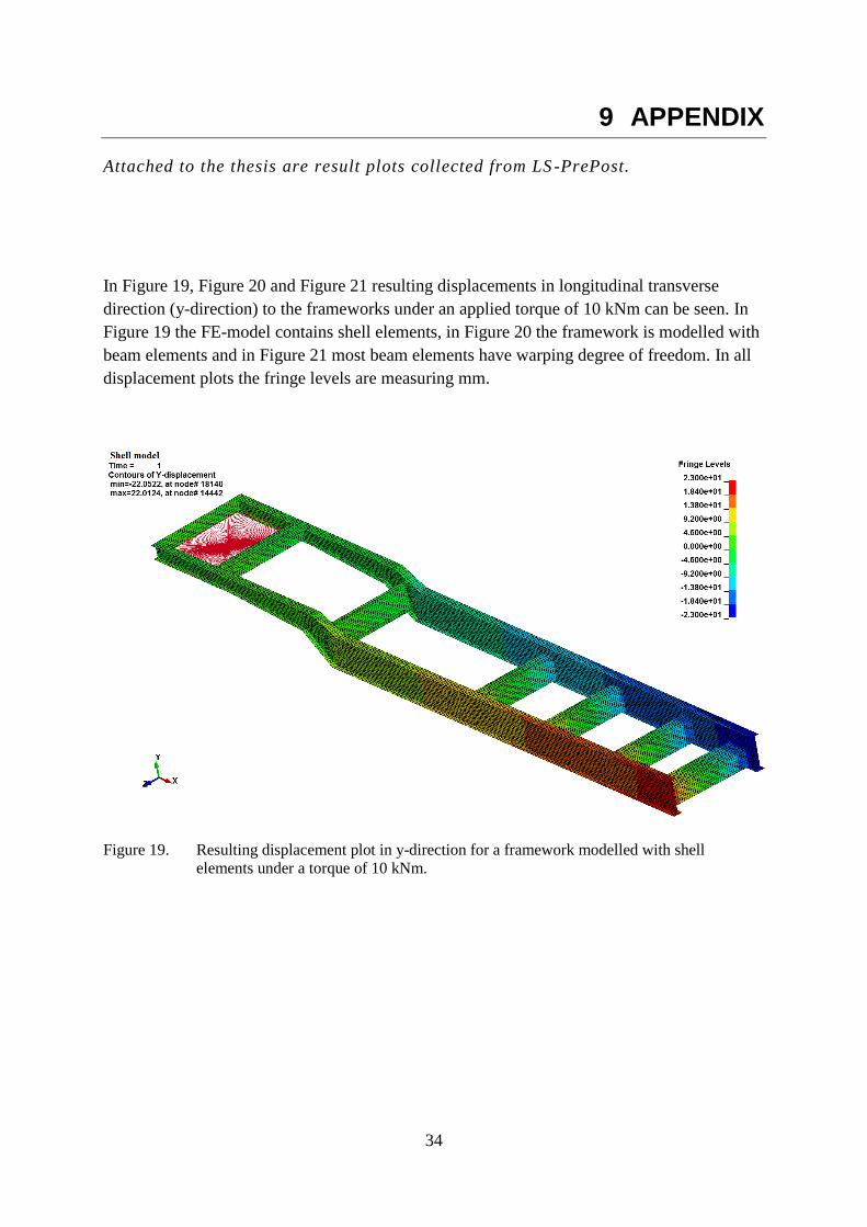
In Figure 19, Figure 20 and Figure 21 resulting displacements in longitudinal transverse
direction (y-direction) to the frameworks under an applied torque of 10 kNm can be seen. In
Figure 19 the FE-model contains shell elements, in Figure 20 the framework is modelled with
beam elements and in Figure 21 most beam elements have warping degree of freedom. In all
displacement plots the fringe levels are measuring mm.
Figure 19. Resulting displacement plot in y-direction for a framework modelled with shell
elements under a torque of 10 kNm.

35
Figure 20. Resulting displacement plot in y-direction for a framework modelled with beam
elements (ELFORM=2) under a torque of 10 kNm.
Figure 21. Resulting displacement plot in y-direction for a framework modelled with mostly
warped beam elements (ELFORM=11) and a few regular beam elements (ELFORM=2)
under a torque of 10 kNm.

36
In Figure 22, Figure 23 and Figure 24 resulting displacements in horizontal transverse
direction (z-direction), for frameworks under an applied torque of 10 kNm can be seen. In
Figure 22 the framework is modelled with shell elements, in Figure 23 the framework is
modelled with beam elements and in Figure 24 the beam elements have a warping degree of
freedom.
Figure 22. Resulting displacement plot in z-direction for a framework modelled with shell
elements under a torque of 10 kNm.
Figure 23. Resulting displacement plot in z-direction for a framework modelled with beam
elements (ELFORM=2) under a torque of 10 kNm.

37
Figure 24. Resulting displacement plot in z-direction for a framework modelled with mostly
warped beam elements (ELFORM=11) and a few regular beam elements (ELFORM=2)
under a torque of 10 kNm.

38
In Figure 25, Figure 26 and Figure 27 resulting displacements in the direction of the length (x-
direction), for frameworks under an applied torque of 10 kNm can be seen. In Figure 25 the
framework is modelled with shell elements, in Figure 26 the framework is modelled with
beam elements and in Figure 27 the beam elements have a warping degree of freedom.
Figure 25. Resulting displacement plot in x-direction for a framework modelled with shell
elements under a torque of 10 kNm.
Figure 26. Resulting displacement plot in x-direction for a framework modelled with beam
elements (ELFORM=2) under a torque of 10 kNm.

39
Figure 27. Resulting displacement plot in x-direction for a framework modelled with mostly
warped beam elements (ELFORM=11) and a few regular beam elements (ELFORM=2)
under a torque of 10 kNm.

40
In Figure 28 the von Mises stress state of the shell model can be observed. The torque applied
is 10 kNm.
Figure 28. The von Mises stress state of a framework modelled with shell elements under an
applied torque of 10 kNm. The values are displayed in MPa.

41