Embed Size (px)
Citation preview
October 24, 2005 Page 1 of 36 Rev D
Parametric Project Monitoring and Control
Performance-Based Progress Assessment and Prediction Mike Ross
Galorath Incorporated 100 North Sepulveda Boulevard
Suite 1801 El Segundo, California 90245
(480) 488-8366 (phone) (480) 488-8420 (fax) [email protected] http://www.galorath.com
Abstract. Performance Measurement (an integral part of Earned Value Management (EVM)) has, over at least the last two decades, become a gold standard process (i.e., best practice) for monitoring and controlling the progress of software development projects. It employs the fundamental measurement-based command/feedback principals of control theory to increase the probability that a project’s actual performance matches its expected (planned) performance; i.e., that a project is delivered on time and within budget or, at least, that there is an early warning of looming disaster. This process is generally well-understood by project managers and reasonably well supported by commercially-available tools. Experience with this process suggests an opportunity for significant process improvement by including established estimation methodology and algorithms as part of the forecasting and re-baselining activities performed during the project monitoring and control process. This paper first reviews the fundamentals of software project management and of Performance Measurement (including some proposed extensions to the notion of earning value) and then proposes a process called Parametric Project Monitoring and Control (PPMC) whereby accepted algorithms currently used for software cost and schedule estimation during the project planning process are incorporated into the forecasting and re-baselining processes to yield a more-realistic time-range prediction of the project’s cost and duration.
October 24, 2005 Page 2 of 36 Rev D
Introduction
Purpose The purpose of this paper is to first review the fundamentals of software project management and of Performance Measurement (including some proposed extensions to the notion of earning value) and then to propose a process called Parametric Project Monitoring and Control (PPMC) whereby accepted algorithms currently used for software cost and schedule estimation during the project planning process are incorporated into the Estimate at Completion (EAC) calculation to yield a more-realistic time-range prediction of the project’s cost and duration.
Scope This paper applies to the project management aspects of the software development process; particularly to those Level 2 process areas referred to in the Carnegie Mellon University Software Engineering Institute’s (SEI) Capability Maturity Model® Integration (CMMI™) for Project Planning, Project Monitoring and Control, and Measurement and Analysis [1]. While the scope and focus of this paper is the software development process, one could imagine how these ideas can be readily applied to hardware and system development as well.
Background Performance Measurement (an integral part of Earned Value Management (EVM)) has, over at least the last two decades, become a gold standard process (i.e., best practice) for monitoring and controlling the progress of software development projects. It employs the fundamental measurement-based command/feedback principals of control theory to increase the probability that a project’s actual performance matches its expected (planned) performance; i.e., that a project is delivered on time and within budget or, at least, that there is an early warning of looming disaster. This process is generally well-understood by project managers and reasonably well supported by commercially-available tools. Experience with this process suggests an opportunity for significant process improvement by including established estimation methodology and algorithms as part of the forecasting and re-baselining activities performed during the Project Monitoring and Control process.
Software Project Management The primary purpose of the software project management process is to ensure that its associated software development project is successful. Success, within this context, is
October 24, 2005 Page 3 of 36 Rev D
assumed to mean achieving or exceeding expectations; i.e., success occurs when the actual outcome matches (within a reasonable tolerance) the expected outcome [4].
The above definition of success, by virtue of its reference to expectations, implies the need for some sort of roadmap or plan; i.e., some sort of description of these expectations in terms of who, what, when, where, how, and why. It follows, then, that one of the software project management process’s primary activities should be planning.
Assuming correspondence between expectations and some sort of project plan, we can now assert that success occurs when the actual outcome matches this plan (within some reasonable tolerance). Ensuring that the actual outcome matches the plan must, therefore, be of primary concern to the software project management process. Ensuring this match implies influencing the actual outcome and/or changing the plan; therefore, one of the software project management process’s primary activities should be controlling.
Influencing the actual outcome is typically achieved by careful initialization, direction, and correction of the software development process and of the environment in which it is performed. Since the software development process is fueled primarily by labor (people), one of the software project management process’s primary activities should be resourcing. Since software development is, indeed, a process, it involves methods, skills/expertise, tools, and task flow. Therefore, the set of software project management process primary activities should also include organizing, training, and equipping.
Finally, once the project is complete, we must deliver the product, determine whether or not the project was a success, and learn from all that was measured and experienced during the project. We therefore suggest that one of the software project management process’s primary activities should be transitioning; transitioning the project’s product to the consumer and transitioning the project’s knowledge and experience to the next project(s).
A useful mental device for remembering the above-described software project management process primary activities is the fact that the first letter of each activity name forms the word PROTECT.
■ Planning – estimating, scheduling
■ Resourcing – interviewing, hiring, motivating
■ Organizing – establishing interpersonal communication paths and rules, mapping resources to tasks
■ Training – teaching, mentoring
■ Equipping – acquiring and allocating equipment, tools, materials, supplies, products etc.
■ Controlling – directing, measuring, correcting and/or replanning
October 24, 2005 Page 4 of 36 Rev D
■ Transitioning – delivering, reviewing, analyzing, archiving
The software project management process, by ensuring project success, is protecting the sponsoring organization’s investment in the project. Or, perhaps (I can’t resist injecting a little gallows humor here), it is protecting the software project manager’s job.
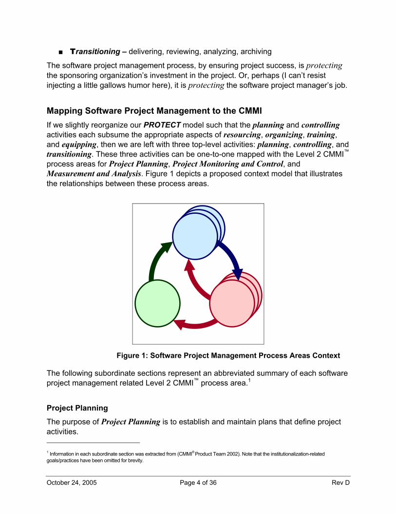
Mapping Software Project Management to the CMMI If we slightly reorganize our PROTECT model such that the planning and controlling activities each subsume the appropriate aspects of resourcing, organizing, training, and equipping, then we are left with three top-level activities: planning, controlling, and transitioning. These three activities can be one-to-one mapped with the Level 2 CMMI™ process areas for Project Planning, Project Monitoring and Control, and Measurement and Analysis. Figure 1 depicts a proposed context model that illustrates the relationships between these process areas.
Figure 1: Software Project Management Process Areas Context
The following subordinate sections represent an abbreviated summary of each software project management related Level 2 CMMI™ process area.1
Project Planning
The purpose of Project Planning is to establish and maintain plans that define project activities. 1 Information in each subordinate section was extracted from (CMMI® Product Team 2002). Note that the institutionalization-related goals/practices have been omitted for brevity.
October 24, 2005 Page 5 of 36 Rev D
Establish Estimates
Estimate the Scope of the Project
Establish Estimates of Work Product and Task Attributes
Define Project Life Cycle
Determine Estimates of Effort and Cost
Develop a Project Plan
Establish the Budget and Schedule
Identify Project Risks
Plan for Data Management
Plan for Project Resources
Plan for Needed Knowledge and Skills
Plan Stakeholder Involvement
Establish the Project Plan
Obtain Commitment to the Plan
Review Plans that Affect the Project
Reconcile Work and Resource Levels
Obtain Plan Commitment
Project Monitoring and Control
The purpose of Project Monitoring and Control is to provide an understanding of the project’s progress so that appropriate corrective actions can be taken when the project’s performance deviates significantly from the plan.
Monitor Project Against Plan
Monitor Project Planning Parameters
Monitor Commitments
Monitor Project Risks
Monitor Data Management
Monitor Stakeholder Involvement
Conduct Progress Reviews
Conduct Milestone Reviews
October 24, 2005 Page 6 of 36 Rev D
Manage Corrective Action to Closure
Analyze Issues
Take Corrective Action
Manage Corrective Action
Measurement and Analysis
The purpose of Measurement and Analysis is to develop and sustain a measurement capability that is used to support management information needs.
Align Measurement and Analysis Activities
Establish Measurement Objectives
Specify Measures
Specify Data Collection and Storage Procedures
Specify Analysis Procedures
Provide Measurement Results
Collect Measurement Data
Analyze Measurement Data
Store Data and Results
Communicate Results
Fundamentals of Software Development
Software Development Taxonomy Terms defined:2
Abstraction – A representation of an idea or concept expressed in a particular medium or language.
Desire – A want or need.
[Software] Requirements – An abstraction of a desire for which computer technology is thought to be a viable solution; the essence of a software product.
Software – An abstraction of a desire expressed as instructions and data in a form that can be acted upon by a computer. 2 Term definitions extracted from [4].
October 24, 2005 Page 7 of 36 Rev D
Process – A set of actions or operations conducing to an end [3].
Software Development Process – A generalized set of related activities that transform desires into software.
Software [Development] Project – A specific instance of a software development process.
Software Product – The primary (deliverable) result of a Software Development Project; the implementation of a software product.
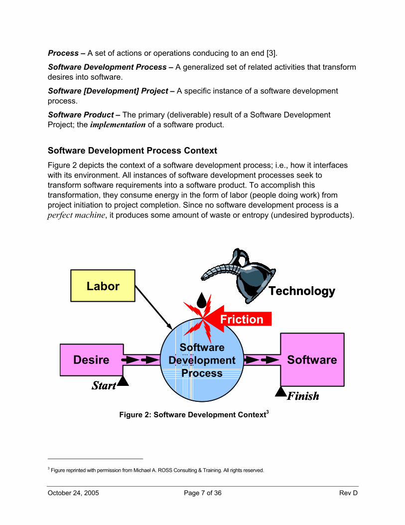
Software Development Process Context Figure 2 depicts the context of a software development process; i.e., how it interfaces with its environment. All instances of software development processes seek to transform software requirements into a software product. To accomplish this transformation, they consume energy in the form of labor (people doing work) from project initiation to project completion. Since no software development process is a perfect machine, it produces some amount of waste or entropy (undesired byproducts).
Desire Software
Labor
StartFinish
SoftwareDevelopment
Process
Technology
Friction
Desire SoftwareDesire Software
LaborLabor
StartFinish
StartFinish
SoftwareDevelopment
Process
TechnologyTechnology
Friction
Figure 2: Software Development Context3
3 Figure reprinted with permission from Michael A. ROSS Consulting & Training. All rights reserved.
October 24, 2005 Page 8 of 36 Rev D
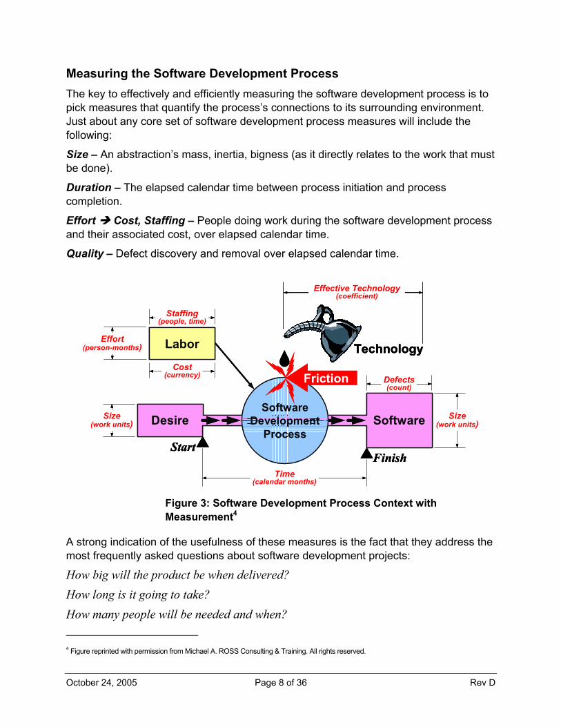
Measuring the Software Development Process The key to effectively and efficiently measuring the software development process is to pick measures that quantify the process’s connections to its surrounding environment. Just about any core set of software development process measures will include the following:
Size – An abstraction’s mass, inertia, bigness (as it directly relates to the work that must be done).
Duration – The elapsed calendar time between process initiation and process completion.
Effort Cost, Staffing – People doing work during the software development process and their associated cost, over elapsed calendar time.
Quality – Defect discovery and removal over elapsed calendar time.
Desire Software
Labor
StartFinish
Effort(person-months)
Size(work units)
Size(work units)
Defects(count)
Time(calendar months)
SoftwareDevelopment
Process
Staffing(people, time)
Cost(currency)
Technology
Friction
Effective Technology(coefficient)
Desire SoftwareDesire Software
LaborLabor
StartFinish
StartFinish
Effort(person-months)
Effort(person-months)
Size(work units)
Size(work units)
Size(work units)
Size(work units)
Defects(count)
Defects(count)
Time(calendar months)
Time(calendar months)
SoftwareDevelopment
Process
Staffing(people, time)
Staffing(people, time)
Cost(currency)
Cost(currency)
TechnologyTechnology
Friction
Effective Technology(coefficient)
Effective Technology(coefficient)
Figure 3: Software Development Process Context with Measurement4
A strong indication of the usefulness of these measures is the fact that they address the most frequently asked questions about software development projects:
How big will the product be when delivered? How long is it going to take? How many people will be needed and when? 4 Figure reprinted with permission from Michael A. ROSS Consulting & Training. All rights reserved.
October 24, 2005 Page 9 of 36 Rev D
How much will it cost? How reliable will the product be when delivered?
Progress Defined
Transforming Desires to Software The fundamental goal (i.e., the root of progress) associated with the software development process is the transformation of a mass of knowledge articulated as a desire into a mass of knowledge articulated as software. While this transformation may, in actuality, exist in a space of many dimensions and directions (bordering on chaotic), we choose to focus on a single dimension we will call progress, the axis or direction of which we will call s .
Progress Position and Change Within dynamic systems, the concept of position is typically used to quantify location within some space relative to some selected reference point. Position is typically represented as a vector quantity; i.e., it consists of both magnitude and direction from some given reference point or point of origin. We have already assumed that our system has only one relevant dimension which we have named progress. Within the progress dimension, we will establish the initial position of the mass of knowledge articulated as a desire (the initial state of the transformation) as being the point of origin of measurement and will measure position relative to this point in the s direction (along the s axis). We will further assume that our system is restricted to the positive side of the s axis; i.e., we will assume the notion of negative position to be undefined.5
Normalized Earned Value Since our system is a transformation from one tangible state (the desire) to another tangible state (the software) with intermediate states being somewhat intangible, we choose unity (1 or 100% complete) to represent the position of the transformation at completion. As previously stated, the initial position of the transformation is assumed to be zero (0% complete). We define any value that represents a specific position on the continuum of intermediate position values as normalized earned value. In other words, if a project’s position in the direction of progress is 0.5 (50% complete), then that project’s normalized earned value is said to be 0.5 or 50%. If a project has been assigned 5 The author acknowledges that this assumption is open to challenge; i.e., that it might be necessary to account for the notion of project digression beyond the initial state. The author, however, chooses to take the more positive viewpoint that what appears, on the surface, to be digression, is actually part of the necessary learning process that is key to any development activity. In other words, while it might not be obvious at the time, you are always better off today than you were yesterday.
October 24, 2005 Page 10 of 36 Rev D
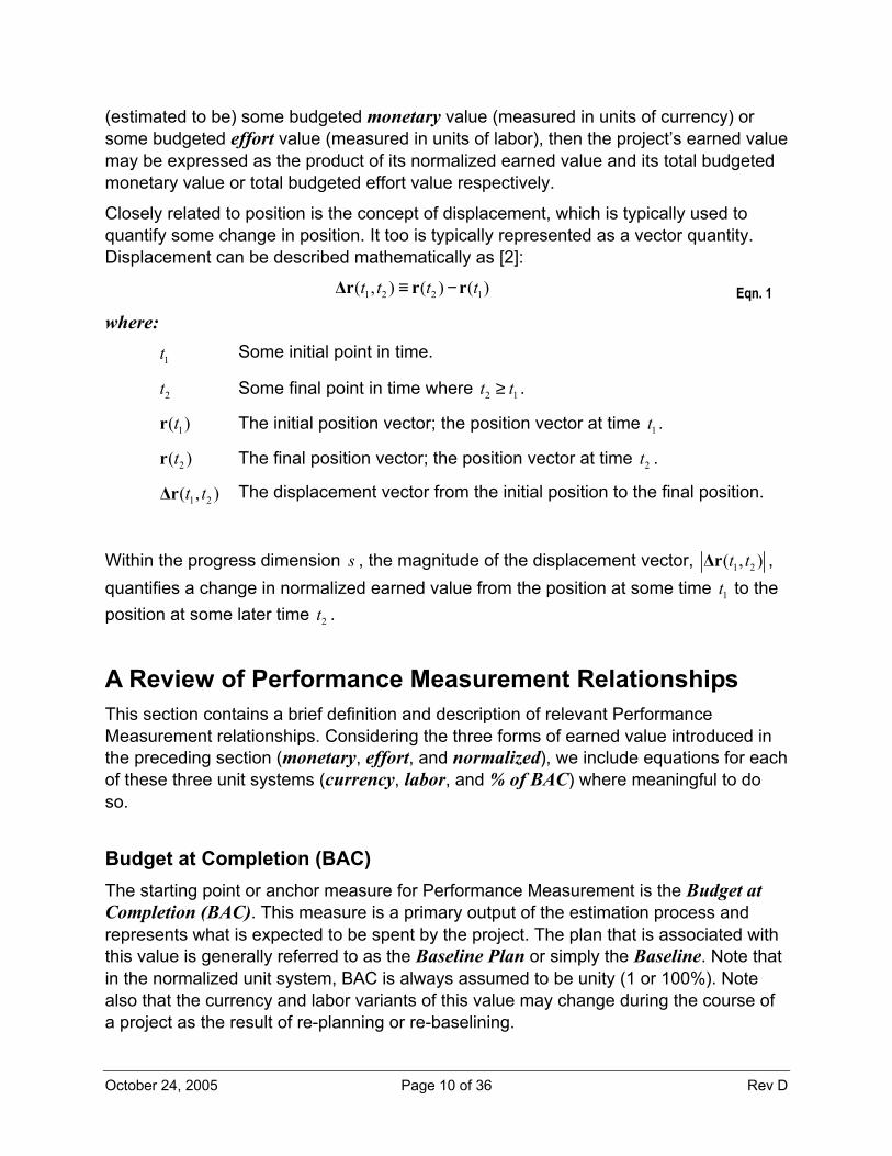
(estimated to be) some budgeted monetary value (measured in units of currency) or some budgeted effort value (measured in units of labor), then the project’s earned value may be expressed as the product of its normalized earned value and its total budgeted monetary value or total budgeted effort value respectively.
Closely related to position is the concept of displacement, which is typically used to quantify some change in position. It too is typically represented as a vector quantity. Displacement can be described mathematically as [2]:
1 2 2 1( , ) ( ) ( )t t t t≡ −∆r r r Eqn. 1
where:
1t Some initial point in time.
2t Some final point in time where 2 1t t≥ .
1( )tr The initial position vector; the position vector at time 1t .
2( )tr The final position vector; the position vector at time 2t .
1 2( , )t t∆r The displacement vector from the initial position to the final position.
Within the progress dimension s , the magnitude of the displacement vector, 1 2( , )t t∆r , quantifies a change in normalized earned value from the position at some time 1t to the position at some later time 2t .
A Review of Performance Measurement Relationships This section contains a brief definition and description of relevant Performance Measurement relationships. Considering the three forms of earned value introduced in the preceding section (monetary, effort, and normalized), we include equations for each of these three unit systems (currency, labor, and % of BAC) where meaningful to do so.
Budget at Completion (BAC) The starting point or anchor measure for Performance Measurement is the Budget at Completion (BAC). This measure is a primary output of the estimation process and represents what is expected to be spent by the project. The plan that is associated with this value is generally referred to as the Baseline Plan or simply the Baseline. Note that in the normalized unit system, BAC is always assumed to be unity (1 or 100%). Note also that the currency and labor variants of this value may change during the course of a project as the result of re-planning or re-baselining.
October 24, 2005 Page 11 of 36 Rev D
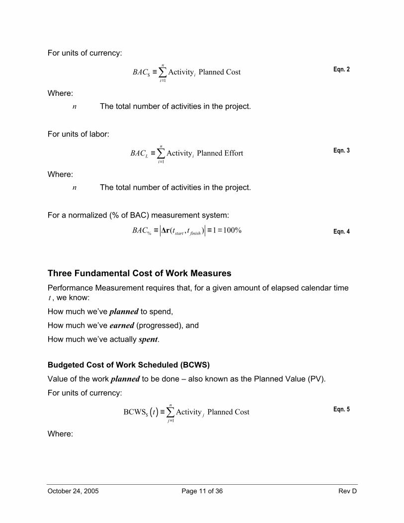
For units of currency:
$1
Activity Planned Costn
ii
BAC=
≡∑ Eqn. 2
Where: n The total number of activities in the project.
For units of labor:
1Activity Planned Effort
n
L ii
BAC=
≡∑ Eqn. 3
Where: n The total number of activities in the project.
For a normalized (% of BAC) measurement system:
% ( , ) 1 100%start finishBAC t t≡ ≡ =∆r Eqn. 4
Three Fundamental Cost of Work Measures Performance Measurement requires that, for a given amount of elapsed calendar time t , we know:
How much we’ve planned to spend,
How much we’ve earned (progressed), and
How much we’ve actually spent.
Budgeted Cost of Work Scheduled (BCWS)
Value of the work planned to be done – also known as the Planned Value (PV).
For units of currency:
( )$1
BCWS Activity Planned Costn
jj
t=
≡∑ Eqn. 5
Where:
October 24, 2005 Page 12 of 36 Rev D
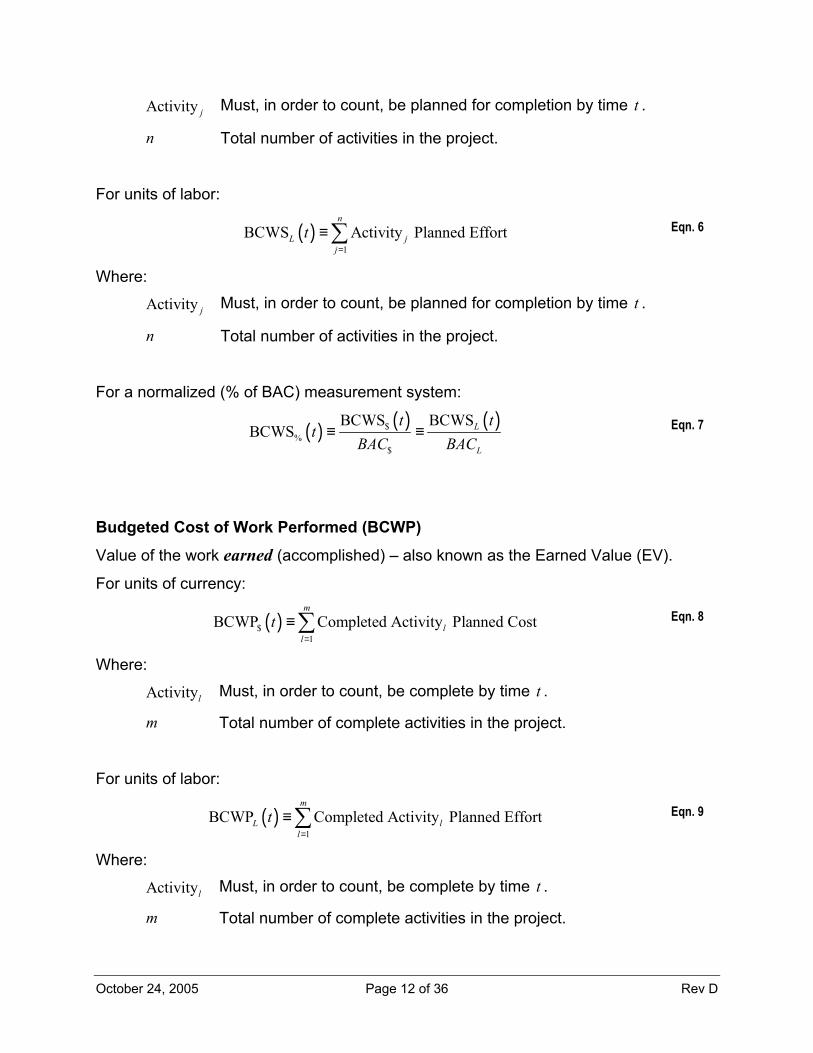
Activity j Must, in order to count, be planned for completion by time t .
n Total number of activities in the project.
For units of labor:
( )1
BCWS Activity Planned Effortn
L jj
t=
≡∑ Eqn. 6
Where:
Activity j Must, in order to count, be planned for completion by time t .
n Total number of activities in the project.
For a normalized (% of BAC) measurement system:
( ) ( ) ( )$%
$
BCWS BCWSBCWS L
L
t tt
BAC BAC≡ ≡ Eqn. 7
Budgeted Cost of Work Performed (BCWP)
Value of the work earned (accomplished) – also known as the Earned Value (EV).
For units of currency:
( )$1
BCWP Completed Activity Planned Costm
ll
t=
≡∑ Eqn. 8
Where:
Activityl Must, in order to count, be complete by time t .
m Total number of complete activities in the project.
For units of labor:
( )1
BCWP Completed Activity Planned Effortm
L ll
t=
≡∑ Eqn. 9
Where:
Activityl Must, in order to count, be complete by time t .
m Total number of complete activities in the project.
October 24, 2005 Page 13 of 36 Rev D
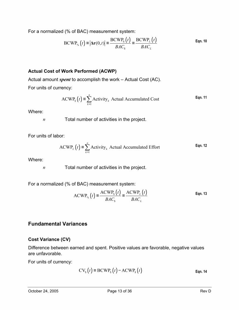
For a normalized (% of BAC) measurement system:
( ) ( ) ( )$%
$
BCWP BCWPBCWP (0, ) L
L
t tt t
BAC BAC≡ ≡ ≡∆r Eqn. 10
Actual Cost of Work Performed (ACWP)
Actual amount spent to accomplish the work – Actual Cost (AC).
For units of currency:
( )$1
ACWP Activity Actual Accumulated Costn
kk
t=
≡∑ Eqn. 11
Where: n Total number of activities in the project.
For units of labor:
( )1
ACWP Activity Actual Accumulated Effort n
L kk
t=
≡∑ Eqn. 12
Where: n Total number of activities in the project.
For a normalized (% of BAC) measurement system:
( ) ( ) ( )$%
$
ACWP ACWPACWP L
L
t tt
BAC BAC≡ ≡ Eqn. 13
Fundamental Variances
Cost Variance (CV)
Difference between earned and spent. Positive values are favorable, negative values are unfavorable.
For units of currency:
( ) ( ) ( )$ $ $CV BCWP ACWPt t t≡ − Eqn. 14
October 24, 2005 Page 14 of 36 Rev D
For units of labor:
( ) ( ) ( )CV BCWP ACWPL L Lt t t≡ − Eqn. 15
For a normalized (% of BAC) measurement system:
( ) ( ) ( )% % %CV BCWP ACWPt t t≡ − Eqn. 16
Schedule Variance (SV)
Difference between earned and planned. Positive values are favorable, negative values are unfavorable.
For units of currency:
( ) ( ) ( )$ $ $SV BCWP BCWSt t t≡ − Eqn. 17
For units of labor:
( ) ( ) ( )SV BCWP BCWSL L Lt t t≡ − Eqn. 18
For a normalized (% of BAC) measurement system:
( ) ( ) ( )% % %SV BCWP BCWSt t t≡ − Eqn. 19
Additional Variances
Budget Variance (BV)
Difference between planned and actual. Positive values are favorable, negative values are unfavorable.
For units of currency:
( ) ( ) ( )$ $ $BV BCWS ACWPt t t≡ − Eqn. 20
For units of labor:
October 24, 2005 Page 15 of 36 Rev D
( ) ( ) ( )BV BCWS ACWPL L Lt t t≡ − Eqn. 21
For a normalized (% of BAC) measurement system:
( ) ( ) ( )% % %BV BCWS ACWPt t t≡ − Eqn. 22
Time Variance (TV)
Difference in elapsed calendar time between time now and time where plan function equals earned function evaluated at time now. Positive values are favorable, negative values are unfavorable.
For units of elapsed calendar time:
( ) ( ) ( ) ( )$ $ % %BCWS BCWP BCWS BCWP BCWS BCWPTVL Lt t t tt t t t t t t= = =≡ − ≡ − ≡ − Eqn. 23
For a normalized (% of BAC) measurement system:
( ) ( )
( )
( )
( )
( )
( )
$ $ % %
$ $ % %
BCWS BCWP BCWS BCWP BCWS BCWP%
BCWS BCWP BCWS BCWP BCWS BCWP
TV L L
L L
t t t
t t t
t t t t t tt
t t t= = =
= = =
− − −≡ ≡ ≡ Eqn. 24
Fundamental Performance Indices
Cost Performance Index (CPI)
Amount earned to amount spent ratio; cost efficiency achieved from project start to time t . Values greater than unity are favorable, values less than unity are unfavorable.
( ) ( )( )
( )( )
( )( )
$ %
$ %
BCWP BCWP BCWPCPI
ACWP ACWP ACWPL
L
t t tt
t t t≡ ≡ ≡ Eqn. 25
Schedule Performance Index (SPI)
Amount earned to amount planned ratio; schedule efficiency achieved from project start to time t . Values greater than unity are favorable, values less than unity are unfavorable.
October 24, 2005 Page 16 of 36 Rev D
( ) ( )( )
( )( )
( )( )
$ %
$ %
BCWP BCWP BCWPSPI
BCWS BCWS BCWSL
L
t t tt
t t t≡ ≡ ≡ Eqn. 26
Additional Performance Indices
Budget Performance Index (BPI)
Amount planned to amount spent ratio; budget efficiency achieved from project start to time t . Values greater than unity are favorable, values less than unity are unfavorable.
( ) ( )( )
( )( )
( )( )
$ %
$ %
BCWS BCWS BCWSBPI
ACWP ACWP ACWPL
L
t t tt
t t t≡ ≡ ≡ Eqn. 27
Time Performance Index (TPI)
Time efficiency achieved from project start to time t . Values greater than unity are favorable, values less than unity are unfavorable.
( ) ( ) ( ) ( )$ $ % %BCWS BCWP BCWS BCWP BCWS BCWPTPI L Lt t tt t tt
t t t= = =≡ ≡ ≡ Eqn. 28
Composite Performance Index (XPI)
Combined cost and schedule efficiency achieved from project start to time t . Values greater than unity are favorable, values less than unity are unfavorable.
( ) ( ) ( )XPI CPI SPIt t t≡ Eqn. 29
Status and Forecasting Metrics
Percent Complete
%Percent Complete BCWP≡ Eqn. 30
October 24, 2005 Page 17 of 36 Rev D
Percent Spent
%Percent Spent ACWP≡ Eqn. 31
Estimate at Completion (EAC)
Expected (predicted) actual cost value when normalized earned value reaches 100%.
EAC Based on Cost Variance (Basic)
For units of currency:
( ) ( )$ $ $EACbasic CVt BAC t≡ − Eqn. 32
For units of labor:
( ) ( )EACbasic CVL L Lt BAC t≡ − Eqn. 33
For a normalized (% of BAC) measurement system:
( ) ( )% % %EACbasic CVt BAC t≡ − Eqn. 34
EAC Based on Cost Performance
For units of currency:
( ) ( )$
$EACcpiCPIBAC
tt
≡ Eqn. 35
For units of labor:
( ) ( )EACcpiCPI
LL
BACtt
≡ Eqn. 36
For a normalized (% of BAC) measurement system:
( ) ( )%
%EACcpiCPIBACt
t≡ Eqn. 37
October 24, 2005 Page 18 of 36 Rev D
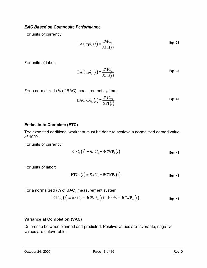
EAC Based on Composite Performance
For units of currency:
( ) ( )$
$EAC xpiXPIBAC
tt
≡ Eqn. 38
For units of labor:
( ) ( )EAC xpiXPI
LL
BACtt
≡ Eqn. 39
For a normalized (% of BAC) measurement system:
( ) ( )%
%EAC xpiXPIBACt
t≡ Eqn. 40
Estimate to Complete (ETC)
The expected additional work that must be done to achieve a normalized earned value of 100%.
For units of currency:
( ) ( )$ $ $ETC BCWPt BAC t≡ − Eqn. 41
For units of labor:
( ) ( )ETC BCWPL L Lt BAC t≡ − Eqn. 42
For a normalized (% of BAC) measurement system:
( ) ( ) ( )% % % %ETC BCWP 100% BCWPt BAC t t≡ − = − Eqn. 43
Variance at Completion (VAC)
Difference between planned and predicted. Positive values are favorable, negative values are unfavorable.
October 24, 2005 Page 19 of 36 Rev D
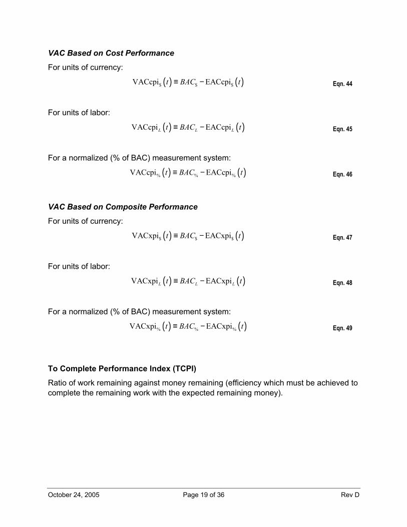
VAC Based on Cost Performance
For units of currency:
( ) ( )$ $ $VACcpi EACcpit BAC t≡ − Eqn. 44
For units of labor:
( ) ( )VACcpi EACcpiL L Lt BAC t≡ − Eqn. 45
For a normalized (% of BAC) measurement system:
( ) ( )% % %VACcpi EACcpit BAC t≡ − Eqn. 46
VAC Based on Composite Performance
For units of currency:
( ) ( )$ $ $VACxpi EACxpit BAC t≡ − Eqn. 47
For units of labor:
( ) ( )VACxpi EACxpiL L Lt BAC t≡ − Eqn. 48
For a normalized (% of BAC) measurement system:
( ) ( )% % %VACxpi EACxpit BAC t≡ − Eqn. 49
To Complete Performance Index (TCPI)
Ratio of work remaining against money remaining (efficiency which must be achieved to complete the remaining work with the expected remaining money).
October 24, 2005 Page 20 of 36 Rev D
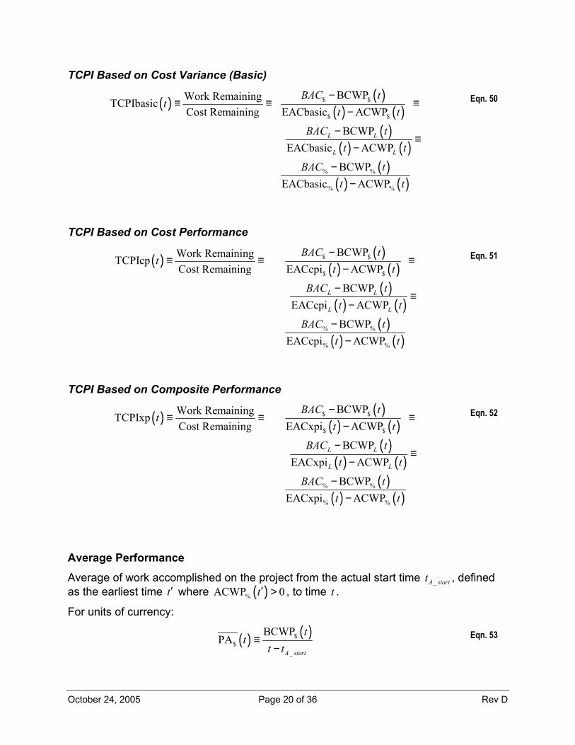
TCPI Based on Cost Variance (Basic)
( ) ( )( ) ( )
( )( ) ( )
( )( ) ( )
$ $
$ $
% %
% %
BCWPWork RemainingTCPIbasic Cost Remaining EACbasic ACWP
BCWP
EACbasic ACWP
BCWPEACbasic ACWP
L L
L L
BAC tt
t t
BAC tt t
BAC tt t
−≡ ≡ ≡
−
−≡
−
−−
Eqn. 50
TCPI Based on Cost Performance
( ) ( )( ) ( )
( )( ) ( )
( )( ) ( )
$ $
$ $
% %
% %
BCWPWork RemainingTCPIcp Cost Remaining EACcpi ACWP
BCWP
EACcpi ACWP
BCWPEACcpi ACWP
L L
L L
BAC tt
t t
BAC tt t
BAC tt t
−≡ ≡ ≡
−
−≡
−
−−
Eqn. 51
TCPI Based on Composite Performance
( ) ( )( ) ( )
( )( ) ( )
( )( ) ( )
$ $
$ $
% %
% %
BCWPWork RemainingTCPIxp Cost Remaining EACxpi ACWP
BCWP
EACxpi ACWP
BCWPEACxpi ACWP
L L
L L
BAC tt
t t
BAC tt t
BAC tt t
−≡ ≡ ≡
−
−≡
−
−−
Eqn. 52
Average Performance
Average of work accomplished on the project from the actual start time _A startt , defined as the earliest time t′ where ( )%ACWP 0t′ > , to time t .
For units of currency:
( ) ( )$$
_
BCWPPA
A start
tt
t t≡
− Eqn. 53
October 24, 2005 Page 21 of 36 Rev D
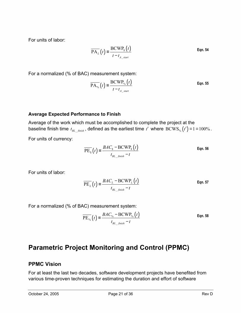
For units of labor:
( ) ( )$
_
BCWPPAL
A start
tt
t t≡
− Eqn. 54
For a normalized (% of BAC) measurement system:
( ) ( )%%
_
BCWPPA
A start
tt
t t≡
− Eqn. 55
Average Expected Performance to Finish
Average of the work which must be accomplished to complete the project at the baseline finish time _BL finisht , defined as the earliest time t′ where ( )%BCWS 1 100%t′ = = .
For units of currency:
( ) ( )$ $$
_
BCWPPE
BL finish
BAC tt
t t−
≡−
Eqn. 56
For units of labor:
( ) ( )_
BCWPPE L L
LBL finish
BAC tt
t t−
≡−
Eqn. 57
For a normalized (% of BAC) measurement system:
( ) ( )% %%
_
BCWPPE
BL finish
BAC tt
t t−
≡−
Eqn. 58
Parametric Project Monitoring and Control (PPMC)
PPMC Vision For at least the last two decades, software development projects have benefited from various time-proven techniques for estimating the duration and effort of software
October 24, 2005 Page 22 of 36 Rev D
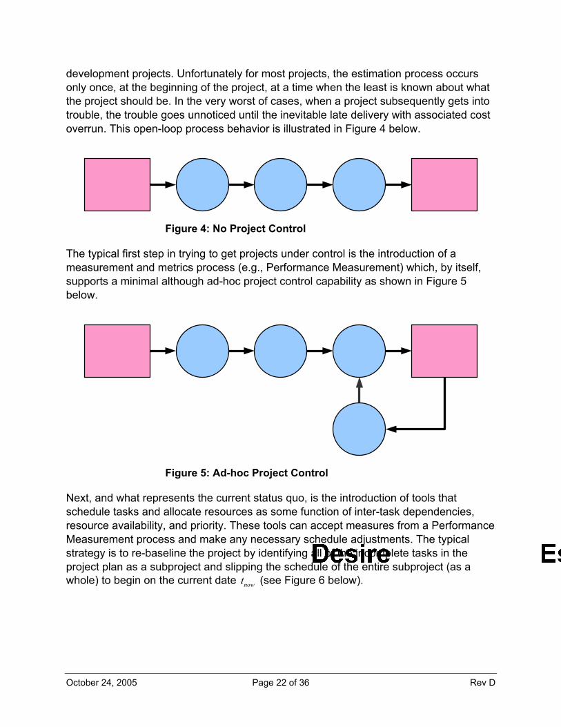
development projects. Unfortunately for most projects, the estimation process occurs only once, at the beginning of the project, at a time when the least is known about what the project should be. In the very worst of cases, when a project subsequently gets into trouble, the trouble goes unnoticed until the inevitable late delivery with associated cost overrun. This open-loop process behavior is illustrated in Figure 4 below.
Figure 4: No Project Control
The typical first step in trying to get projects under control is the introduction of a measurement and metrics process (e.g., Performance Measurement) which, by itself, supports a minimal although ad-hoc project control capability as shown in Figure 5 below.
Figure 5: Ad-hoc Project Control
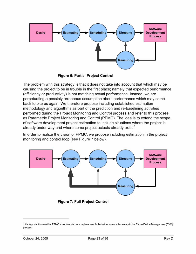
Next, and what represents the current status quo, is the introduction of tools that schedule tasks and allocate resources as some function of inter-task dependencies, resource availability, and priority. These tools can accept measures from a Performance Measurement process and make any necessary schedule adjustments. The typical strategy is to re-baseline the project by identifying all of the incomplete tasks in the project plan as a subproject and slipping the schedule of the entire subproject (as a whole) to begin on the current date nowt (see Figure 6 below).
October 24, 2005 Page 23 of 36 Rev D
SoftwareDevelopment
ProcessEstimating Scheduling DirectingDesire
Measuring
Figure 6: Partial Project Control
The problem with this strategy is that it does not take into account that which may be causing the project to be in trouble in the first place; namely that expected performance (efficiency or productivity) is not matching actual performance. Instead, we are perpetuating a possibly erroneous assumption about performance which may come back to bite us again. We therefore propose including established estimation methodology and algorithms as part of the prediction and re-baselining activities performed during the Project Monitoring and Control process and refer to this process as Parametric Project Monitoring and Control (PPMC). The idea is to extend the scope of software development project estimation to include situations where the project is already under way and where some project actuals already exist.6
In order to realize the vision of PPMC, we propose including estimation in the project monitoring and control loop (see Figure 7 below).
SoftwareDevelopment
ProcessEstimating Scheduling DirectingDesire
Measuring
Figure 7: Full Project Control
6 It is important to note that PPMC is not intended as a replacement for but rather as complementary to the Earned Value Management (EVM) process.
October 24, 2005 Page 24 of 36 Rev D
Extending the Notion of Quantifying Progress (Earning Value) Within the realm of Performance Measurement, one criticism that routinely surfaces is the sometimes arbitrary manner in which progress or value (percent complete) is credited to activities within a project or to the project as a whole. The result of this arbitrariness is sometimes referred to as the “90% complete 90% of the time” syndrome. This paper proposes a four-dimensional (4-D) approach for assigning progress to the development of each program/application (Computer Software Configuration Item (CSCI)) that is part of the project. The first dimension is Software Development Life Cycle (SDLC) primary activity completion for the development of a specific program/application (CSCI). Each SDLC primary activity7, in turn, is assigned progress according to a weighted combination of three other dimensions: artifact completion, milestone completion, and defect discovery / removal.
Program/Application (CSCI) Progress
( )%BCWP t for each program/application (CSCI) is computed as the normalized weighted sum of the applicable SDLC primary activities’ completion percentage. The weighting scheme is directly derived from the effort-to-activity allocation defined in the project’s baseline plan.
SDLC Primary Activity Completion
During the project monitoring and control process, the completion percentage for each SDLC primary activity is computed as the normalized weighted sum of its artifacts completed, its milestones completed, and its associated number of defects discovered and defects removed.
Artifact Completion
As part of the project planning process, a list of artifact types is identified and each type is assigned to the appropriate SDLC primary activity. Each artifact type is weighted according to its relative contribution to the completion of its associated primary activity. Additionally, as part of the project planning process, the total number of artifacts of each type is estimated for each program/application (CSCI). These totals are used to determine the relative weighted contribution of each completed artifact to the completion of its associated SDLC primary activity.
During the project monitoring and control process, the total number of completed artifacts of each type are periodically and/or aperiodically measured and recorded.
7 An example of a set of SDLC primary activities is System Requirements Design, Software Requirements Analysis, Preliminary Design, Detailed Design, Code & Unit Test, Component Integration & Test, Program Test, System Integration thru Operational Test & Evaluation. There are various SDLCs, each with its own unique set of primary activities.
October 24, 2005 Page 25 of 36 Rev D
Milestone Completion
As part of the project planning process, a list of milestones (events) is identified and each is assigned to the appropriate SDLC primary activity. Each milestone is weighted according to its relative contribution to the completion of its associated primary activity.
During the project monitoring and control process, milestone completion state is periodically/aperiodically determined and recorded.
Defect Discovery / Removal
As part of the project planning process, an estimate is made for each program/application (CSCI) of its total theoretical number defects. This body of defects is then twice distributed over elapsed calendar time; once according discovery and once according to removal. The body of defects is also proportionally distributed across the set of SDLC primary activities according to each activity’s corresponding effort allocation. The total number of defects allocated to each SDLC primary activity is used to determine the relative weighted contribution of each discovered and removed defect to the completion of its associated SDLC primary activity.
During the PPMC process, the total numbers of discovered and of removed defects for each SDLC primary activity are periodically/aperiodically measured and recorded.
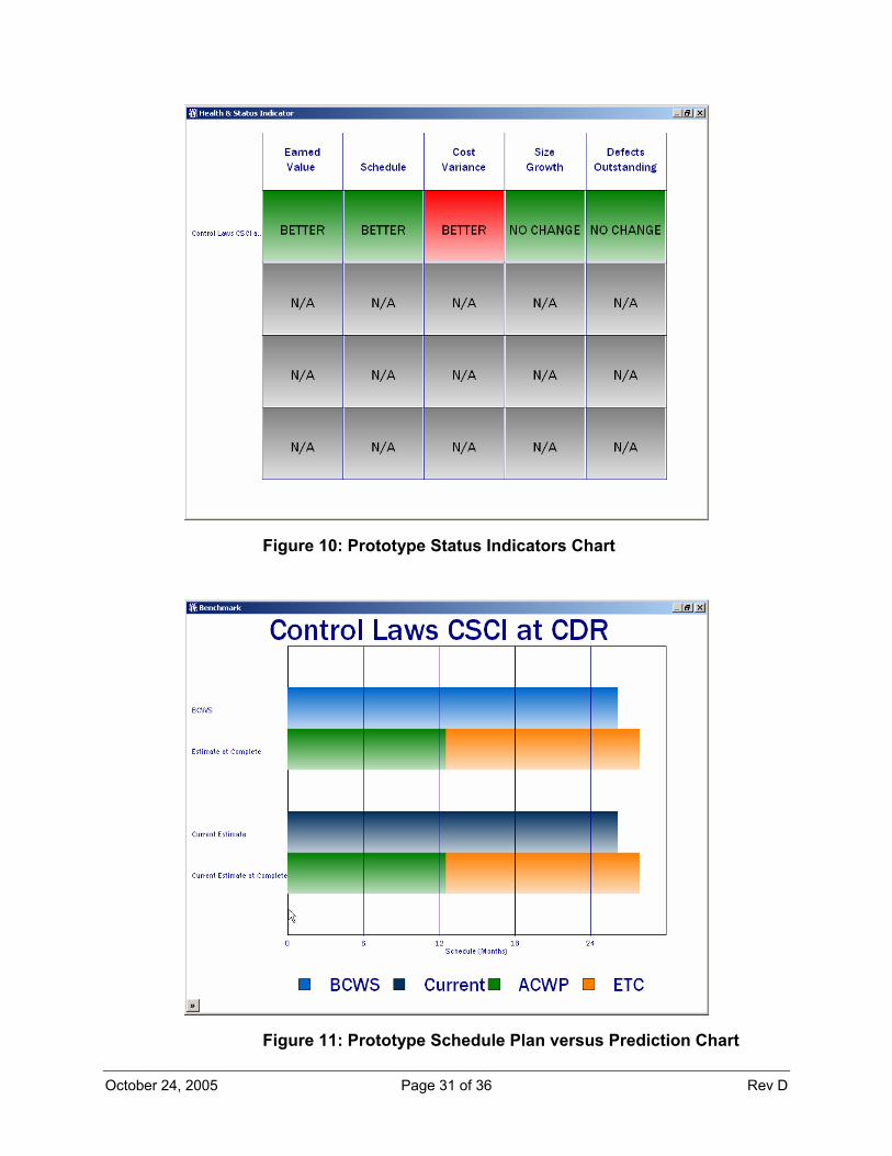
At-a-Glance Status Indication of Measures and Metrics The traffic signal metaphor has become a fairly commonplace strategy to indicate Work Breakdown Structure (WBS) individual task status (red, yellow, green). Since status can be tracked as a function of elapsed calendar time, the notion of status is often-times supplemented by the inclusion of status trend (better, no change, worse). We propose to extend this strategy to include several measures and metrics associated with each program/application (CSCI) that are managed as part of PPMC. These measures and metrics include:8
Cost Variance and Cost Performance Index
Schedule Variance and Schedule Performance Index
Budget Variance and Budget Performance Index
Time Variance and Time Performance Index
Size Growth [4]
Size Uncertainty Convergence [4]
Defect Discovery Variance
Defect Removal Variance 8 This is an evolving list of measures and metrics and is expected to grow as experience is gained applying PPMC to real projects.

October 24, 2005 Page 26 of 36 Rev D
Control Limits Earlier in this paper we defined success to mean achieving or exceeding expectations and asserted that success occurs when the actual outcome matches, within a reasonable tolerance, the expected outcome. In the preceding section we proposed quantifying measurement and metric status using the traffic signal metaphor with trend supplement. In order to realize the traffic signal metaphor for a given measure or metric, we must define all the transitions between green and yellow and between yellow and red. We propose to call these transitions control limits and include them as part of our PPMC process in order to link the notion of reasonable tolerance to the notion of status.
We now propose the following definition for the set of control limits associated with a particular measure or metric where the particular measure or metric can be expressed as a function of elapsed calendar time:9
_ __ __ __ _
control_limit_set upper_yellow to red_control_limitupper_green to yellow_control_limitlower_green to yellow_control_limitlower_yellow to red_control_limit
≡
Eqn. 59
[ ]_ _upper_yellow to red_control_limit control_limit_segment
control_limit_segment≡
K Eqn. 60
[ ]_ _upper_green to yellow_control_limit control_limit_segment
control_limit_segment≡
K Eqn. 61
[ ]_ _upper_yellow to red_control_limit control_limit_segment
control_limit_segment≡
K Eqn. 62
[ ]_ _upper_yellow to red_control_limit control_limit_segment
control_limit_segment≡
K Eqn. 63
_ __
control_limit_segment starting month numberscale factoroffset
≡
Eqn. 64
Note that _ _ 0starting month number = indicates both a null control_limit_segment and the last control_limit_segment in a list.
The control_limit_segment function ( )u j it for the thj control_limit_segment of a particular control_limit in a _control_limit set associated with a particular measure or metric that is
9 The author acknowledges that the “perfect” control limit schema would allow specification as any function of elapsed calendar time. The proposed schema represents a compromise between flexibility and computational complexity.
October 24, 2005 Page 27 of 36 Rev D
a function of elapsed calendar time ( )m it and evaluated at the thi month into the project is defined as:
( ) ( ) ( )u mj i j i jt a t b= + Eqn. 65
Where: m One more than the count of whole months in the range startt to finisht
where m ∈ ¥ . n The count of control limit segments in a particular control limit where
n ∈ ¥ . i Month number where [ ]1,i m∈ ∩¥ .
j Control limit segment index where [ ]* 0,j n∈ ∩¢
it Quantum elapsed calendar time from startt to i months into the project.
ja Scale factor of the thj control limit segment.
jb Offset of the thj control limit segment; must be scaled in the same units as is ( )m it .
( )m it A particular measure or metric defined as a function of elapsed calendar time it .
( )u j it thj control limit segment value for a particular control limit as a function
of elapsed calendar time it .
Performance-Based Forecasting and Re-Baselining At the heart of the PPMC vision is the desire to forecast the final project outcome. We have already proposed the idea of including the estimation process and all of its algorithmic strength in the forecasting process. The question now becomes, “How can we do that?” The following subordinate sections contain a set of process steps that support the creation of a new project plan (estimate) that, by its nature, represents a performance-based forecast and, therefore, represents a reasonable new baseline plan (re-baseline). A strategic goal of PPMC is to eventually automate as many steps in this process as are reasonably possible.
October 24, 2005 Page 28 of 36 Rev D
Step 1: Start a New Estimate
Use the current baseline as the starting point for a new estimate.
Step 2: Update Size Estimate
Revisit all of the assumptions (Basis of Estimate) associated with the current estimate of and uncertainty around software size. Include other sizing techniques, if appropriate, in order to improve sizing accuracy. Make changes where appropriate.
Step 3: Update Technology Assumptions
Revisit all Knowledge Base and technology parameter assumptions that formed the Basis of Estimate for the current baseline. Align Knowledge Base selections and technology parameter settings with what has actually happened to date on the project. Make changes where appropriate.
Step 4: Update Schedule Assumptions
Revisit the project start date and any assumptions about the time-effort tradeoff solution (i.e., minimum time versus optimal effort, schedule constraints, etc.). Make any changes where appropriate.
Step 5: Update Staffing Assumptions
Specify staffing constraints from project start to time now that match (as close as possible) the actual staffing profile to date. Revisit future staffing assumptions from time now and make adjustments where appropriate.
Step 6: Update Labor Rate and FTE Assumptions
Revisit all labor rates as well as the definition of a Full Time Equivalent person (typically specified as number of labor-hours per labor-month). Make any changes where appropriate.
Step 7: Time Now Calibration
This step assumes that the estimation model or process being used can be calibrated by making adjustments to one or more calibration coefficients. We propose iteratively adjusting each calibration coefficient with the goal of creating a plan that corresponds with actual performance (BCWP) and actual expenditure (ACWP) to date. We propose a reasonable test for this correspondence to be performance indices (BPI, CPI, SPI, TPI) approaching unity. Practically speaking, we are creating a new plan that matches
October 24, 2005 Page 29 of 36 Rev D
what has already happened and uses established estimation relationships to predict what is likely to happen from time now considering what has already happened up to time now.
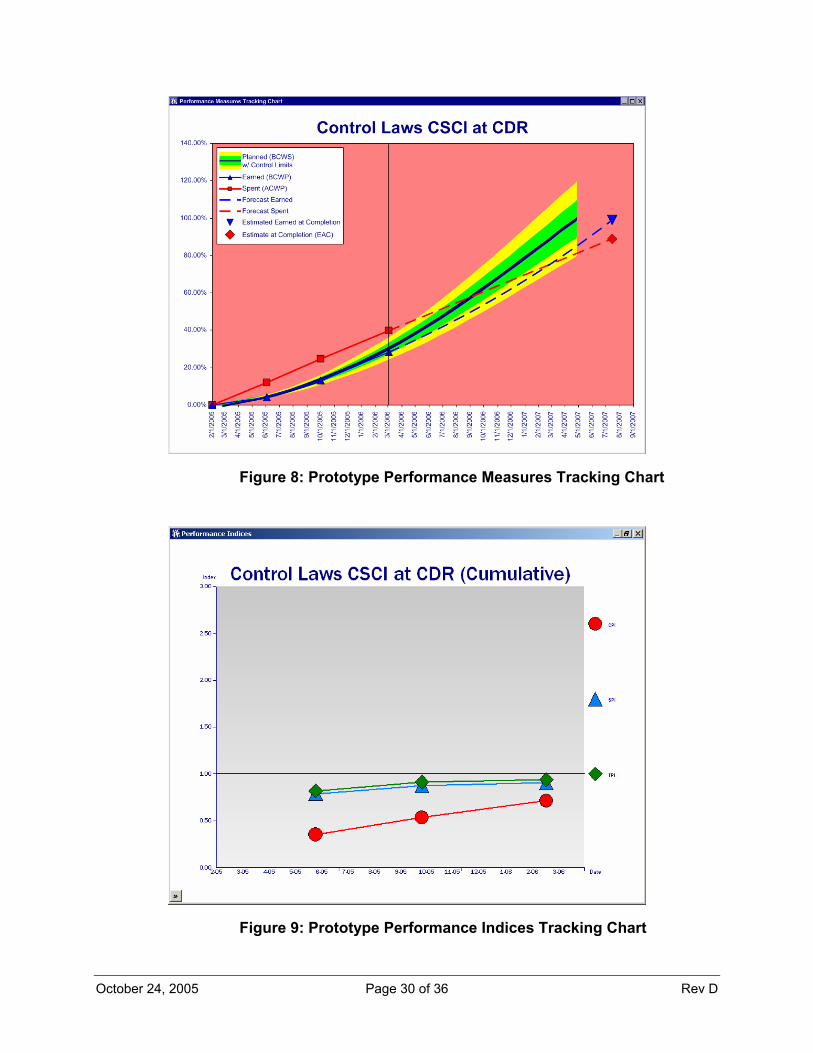
Step 8: Communicate the Results
Use an appropriate set of charts and reports to present the results of the forecasting process. A chart that is particularly useful for this purpose is of the type shown in Figure 8.
Step 9: Re-Baseline the Project
If warranted by project expectations, goals, and commitments and upon approval by appropriate authority, replace the current baseline with the current (new) estimate and track against this new baseline.
Communicating Performance Measurement Information
PPMC Outputs
One of the primary goals of PPMC is to provide adequate supporting documentation (charts and reports) to support the software project management process and to satisfy stakeholder needs. Figure 8 through Figure 14 show prototypical examples of charts and reports that can be used for such a purpose.
October 24, 2005 Page 30 of 36 Rev D
Figure 8: Prototype Performance Measures Tracking Chart
Figure 9: Prototype Performance Indices Tracking Chart
October 24, 2005 Page 31 of 36 Rev D
Figure 10: Prototype Status Indicators Chart
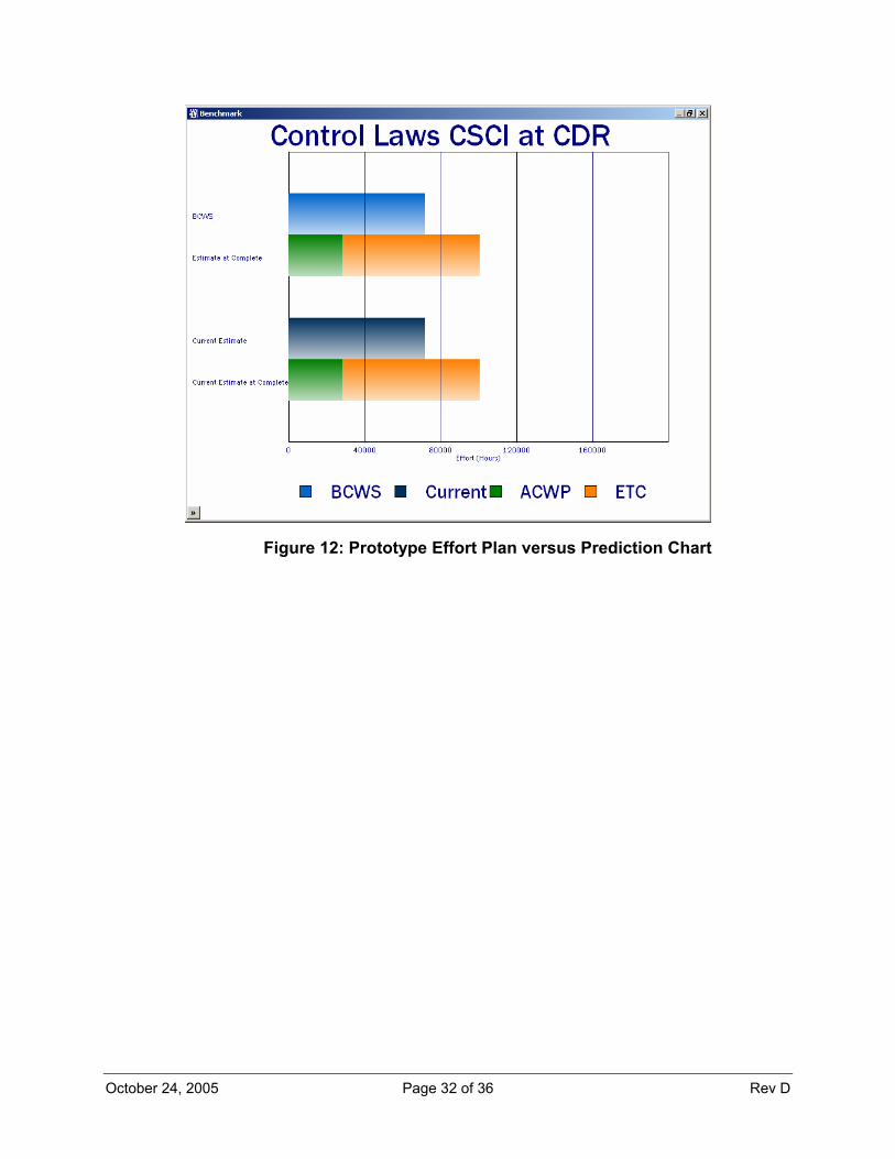
Figure 11: Prototype Schedule Plan versus Prediction Chart
October 24, 2005 Page 32 of 36 Rev D
Figure 12: Prototype Effort Plan versus Prediction Chart
October 24, 2005 Page 33 of 36 Rev D
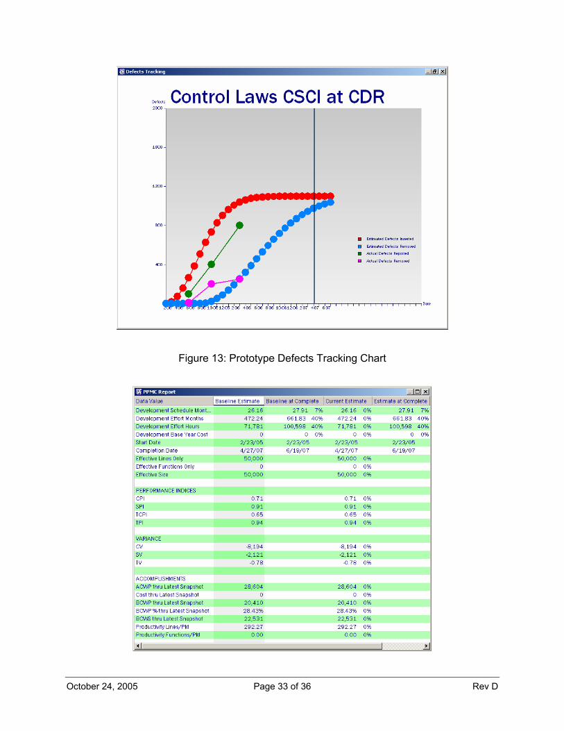
Figure 13: Prototype Defects Tracking Chart
October 24, 2005 Page 34 of 36 Rev D
Figure 14: Prototype PPMC Report
Summary and Conclusion
Purpose Revisited This paper has reviewed the fundamentals of software project management and of Performance Measurement (including proposed extensions) and then examined a proposed process called Parametric Project Monitoring and Control (PPMC) whereby accepted algorithms currently used for software cost and schedule estimation during the project planning process are incorporated into the forecasting and re-baselining processes to yield a more-realistic time-range prediction of a project’s cost and duration.
Areas of Future Study The following are suggested opportunities for improving PPMC:
Identify new measures and metrics that can provide better insight into project health and status.
Investigate methods for automating the Performance-Based Forecasting and Re-Baselining Process. Regarding the iterative calibration process, it might be possible to develop a system of equations that combine the fundamental software estimation equations with the equations for calculating Performance Measurement’s performance indices such that the calibration coefficients could be resolved directly; i.e., avoiding the iterative guessing process.
Develop new graphic and tabular representations of the measures and metrics data that improve communicating a project’s health and status.
Investigate the idea of some sort of project diagnostic expert system that would combine PPMC measures and metrics and provide a list of suggested potential project problems that are indicated by the given values of these measures and metrics.
References [1] CMMI® Product Team, Capability Maturity Model® Integration (CMMI™),
Version 1.1, Pittsburgh, PA: Software Engineering Institute, Carnegie Mellon University, 2002.
[2] Halliday, D., Resnick, R., Physics: Parts 1 & 2, Third Edition, John Wiley & Sons, New York, NY, 1997.
October 24, 2005 Page 35 of 36 Rev D
[3] Mish, F. (Editor in Chief), Merriam-Webster’s Collegiate Dictionary, Tenth Edition, Merriam-Webster, Incorporated, Springfield, MA, 1999.
[4] Ross, M., “Managing Software Size,” Proc. Joint ISPA / SCEA 2003 Conference, June 2003.
October 24, 2005 Page 36 of 36 Rev D
Biography Michael A. Ross has over 30 years of practical experience in software engineering as a developer, manager, process champion, consultant, instructor, and award-winning international speaker.
Mr. Ross is currently the Chief Engineer of Galorath Incorporated, makers of the SEER suite of estimation tools, where, for the past three years, he has been responsible for the advancement and realization of the technology aspects of Galorath’s mission and vision.
Prior to joining Galorath, Mr. Ross was Vice President of Education Services for Quantitative Software Management, Inc. (makers of the SLIM suite of software estimating tools). He was responsible for the development and delivery of all QSM training. During his seven-year tenure with QSM, he served as one of the company’s primary consultants and analysts working with Fortune 500 companies and government agencies in the areas of software measurement, sizing, estimating, tracking, forecasting, and benchmarking.
Mr. Ross, during 17 years with Honeywell Air Transport Systems (formerly Sperry Flight Systems) and 2 years with Tracor Aerospace, developed or managed the development of embedded software for avionics systems installed various commercial airplanes including the Boeing 737-500, 757, 767, 777, the Douglas MD-11, the Lockheed L1011-500, the British Aerospace BAe-146, the Airbus A320; and for expendable countermeasures systems installed in various military aircraft and missiles. He also co-founded Honeywell Air Transport Systems’ process improvement team (later to become its SEPG), served as its focal for software project management process improvement, and served as a Honeywell corporate SEI CMM assessor.
Mr. Ross did his undergraduate work at the United States Air Force Academy and Arizona State University, receiving a Bachelor of Science in Computer Engineering. He is a member of the Project Management Institute (PMI), the Institute of Electrical and Electronics Engineers (IEEE), the International Function Points Users Group (IFPUG), the International Society of Parametric Analysts (ISPA), the Society of Cost Estimating and Analysis (SCEA), the Arizona Software Association, and the Phoenix area Software Process Improvement Network.