Parametric study of the performance of a turbocharged compression

Simulation

Simulation: Transactions of the Society for

Modeling and Simulation International

2014, Vol. 90(12) 1375–1384

� 2014 The Author(s)

DOI: 10.1177/0037549714557046

sim.sagepub.com

Parametric study of the performanceof a turbocharged compressionignition engine

Brahim Menacer and Mostefa Bouchetara

AbstractIn this study, the thermodynamic performance of a turbocharged compression ignition engine with heat transfer and fric-tion term losses was analyzed. The purpose of this work was to provide a flexible thermodynamic model based on thefilling-and-emptying approach for the performance prediction of a four-stroke turbocharged compression ignition engine.To validate the model, comparisons were made between results from a computer program developed using FORTRANlanguage and the commercial GT-Power software operating under different conditions. The comparisons showed thatthere was a good concurrence between the developed program and the commercial GT-Power software. We also stud-ied the influence of several engine parameters on brake power and effective efficiency. The range of variation of the rota-tional speed of the diesel engine chosen extended from 800 to 2100 rpm. By analyzing these parameters with regard totwo optimal points in the engine, one relative to maximum power and another to maximum efficiency, it was found thatif the injection timing is advanced, so the maximum levels of pressure and temperature in the cylinder are high.

KeywordsThermodynamic, combustion, turbocharged compression ignition engine, GT-Power, performance optimization, filling-and-emptying method

1. Introduction

More than a century after its invention by Dr Rudolf

Diesel, the compression ignition engine remains the most

efficient internal combustion engine for ground vehicle

applications. Thermodynamic models (zero-dimensional)

and multi-dimensional models are the two types of models

that have been used in internal combustion engine simula-

tion modeling. Nowadays, trends in combustion engine

simulations are towards the development of comprehen-

sive multi-dimensional models that accurately describe the

performance of engines at a very high level of detail.

However, these models need a precise experimental input

and substantial computational power, which makes the

process significantly complicated and time-consuming.1

On the other hand, zero-dimensional models, which are

mainly based on energy conservation (first law of thermo-

dynamics) are used in this work due to their simplicity and

being less time-consuming in the program execution, and

their relatively accurate results.2 There are many modeling

approaches to analysis and optimization of the internal

combustion engine. Angulo-Brown et al.1 optimized the

power of the Otto and Diesel engines with friction loss

with finite duration cycle. Chen et al.2 derived the relation-

ships of correlation between net power output and the effi-

ciency for Diesel and Otto cycles; there are thermal losses

only on the transformations in contact with the sources

and the heat sinks other than isentropic. Merabet et al.3

proposed a model for which thermal loss is represented

more classically in the form of a thermal conductance

between the mean temperature of gases on each transfor-

mation, V = constant and p = constant, compared to the

wall temperature (Twall). Among the objectives of this

work was to compare the simulation results of the perfor-

mance of a six-cylinder, direct-injection, turbocharged

compression ignition engine using an elaborate calculation

code in FORTRAN with GT-Power software. We also

Department of Mechanical Engineering, University of Sciences and

Technology of Oran, Algeria

Corresponding author:

Brahim Menacer, Department of Mechanical Engineering, University of

Sciences and Technology of Oran, BP 1505 El-MNAOUER, 31000 Oran,

Algeria.

Email [email protected]

studied the influence of certain important thermodynamic

and geometric engine parameters on the brake power, on

the effective efficiency, and also on pressure and tempera-

ture of the gases in the combustion chamber.

2. Diesel engine modeling

There are three essential steps in the mathematical model-

ing of the internal combustion engine:4 (1) thermodynamic

models based on first and second law analysis, which have

been used since 1950 to help engine design or turbocharger

matching and to enhance engine processes understanding;

(2) empirical models based on input–output relations intro-

duced in early 1970s for primary control investigation; (3)

nonlinear models physically based for both engine simula-

tion and control design. Engine modeling for control tasks

involves researchers from different fields, mainly control

and physics. As a consequence, several specific nomina-

tions may designate the same class of model in accordance

with the framework. To avoid any misunderstanding, we

classify models within three categories with terminology

adapted to each field as follows.

1. Thermodynamic-based models or knowledge (so-

called ‘‘white box’’) models for nonlinear, physi-

cally based models suitable for control.

2. Nonthermodynamic models or ‘‘black-box’’ models

for experimental input–output models.

3. Semiphysical approximate models or parametric

(‘‘gray box’’) models. This is an intermediate cate-

gory; here, models are built with equations derived

from physical laws of which parameters (masses,

volume, inertia, etc.) are measured or estimated

using identification techniques.

The next section focuses on category 1, with greater inter-

est on thermodynamic models. For the second and third

classes of models see Guzzella and Amstutz.5

2.1. Thermodynamic-based engine model

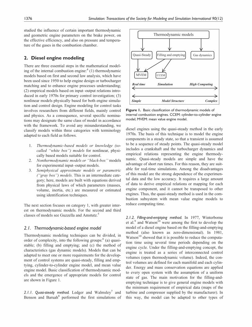
Thermodynamic modeling techniques can be divided, in

order of complexity, into the following groups:6 (a) quasi-

stable; (b) filling and emptying; and (c) the method of

characteristics (gas dynamic models). Models that can be

adapted to meet one or more requirements for the develop-

ment of control systems are quasi-steady, filling and emp-

tying, cylinder-to-cylinder engine model, and mean value

engine model. Basic classification of thermodynamic mod-

els and the emergence of appropriate models for control

are shown in Figure 1.

2.1.1. Quasi-steady method. Ledger and Walmsley7 and

Benson and Baruah8 performed the first simulations of

diesel engines using the quasi-steady method in the early

1970s. The basis of this technique is to model the engine

components in a steady state, so that a transient is assumed

to be a sequence of steady points. The quasi-steady model

includes a crankshaft and the turbocharger dynamics and

empirical relations representing the engine thermody-

namic. Quasi-steady models are simple and have the

advantage of short run times. For this reason, they are suit-

able for real-time simulations. Among the disadvantages

of this model are the strong dependence of the experimen-

tal data and the low accuracy. It requires a large amount

of data to derive empirical relations or mapping for each

engine component, and it cannot be transposed to other

engines. Thus, the quasi-steady method is used in the com-

bustion subsystem with mean value engine models to

reduce computing time.

2.1.2. Filling-and-emptying method. In 1977, Winterborne

et al.9 and Watson10 were among the first to develop the

model of a diesel engine based on the filling-and-emptying

method (also known as zero-dimensional). In 1981,

Watson10 showed that it is possible to reduce the computa-

tion time using several time periods depending on the

engine cycle. Under the filling-and-emptying concept, the

engine is treated as a series of interconnected control

volumes (open thermodynamic volume). Indeed, the con-

trol volumes are defined for each manifold and each cylin-

der. Energy and mass conservation equations are applied

to every open system with the assumption of a uniform

state of gas. The main motivation for the filling-and-

emptying technique is to give general engine models with

the minimum requirement of empirical data (maps of the

turbine and compressor supplied by the manufacturer). In

this way, the model can be adapted to other types of

Model StructureSimple

Real time Simulation High Computing

Thermodynamic models

Filling and emptyingQuasi-Steady

CCEMMVEM

Gas dynamics

Complex

Figure 1. Basic classification of thermodynamic models ofinternal combustion engines. CCEM: cylinder-to-cylinder enginemodel; MVEM: mean value engine model.

1376 Simulation: Transactions of the Society for Modeling and Simulation International 90(12)

engines with minimal effort. The filling-and-emptying

model shows good prediction of engine performance under

steady-state and transient conditions and provides informa-

tion about parameters known to affect pollutant or noise.

However, assumption of uniform state of gas covers up

complex acoustic phenomena (resonance). Wave effects

inside the manifold can affect engine performance and,

therefore, the error introduced by the filling-and-emptying

method must be considered.

2.1.3. Method of characteristics (or gas dynamic models). The

method of characteristics is a very powerful method to

access accurately parameters such as the equivalence ratio

or the contribution to the overall noise sound level of the

intake and the exhaust manifold or the amplitudes of the

pressure fluctuations in the tubes according to their dia-

meter. Its advantage is effectively understanding the

mechanism of the phenomena that happen in a manifold11

and it allows one to obtain accurately laws of evolution of

pressure, speed, and temperature manifolds at any point,

depending on the time, but the characteristic method

requires a much more important calculation program, and

the program’s complexity increases widely with the num-

ber of singularities to be treated.

3. General equation of the model

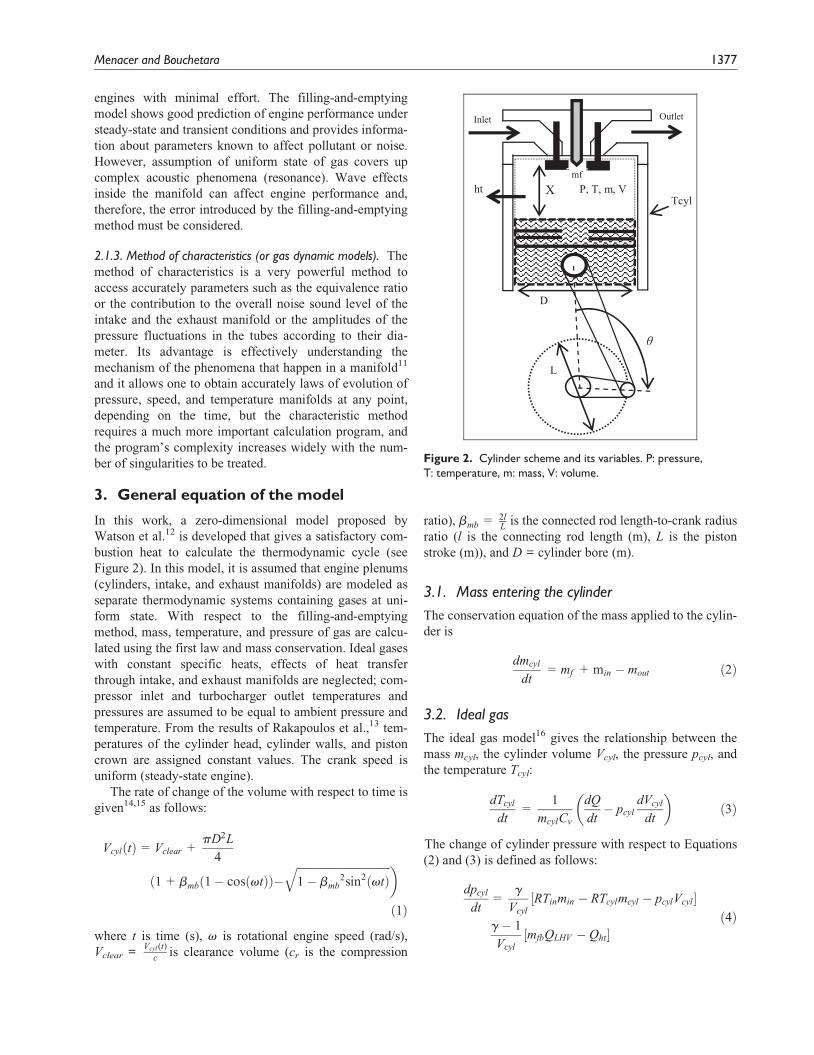
In this work, a zero-dimensional model proposed by

Watson et al.12 is developed that gives a satisfactory com-

bustion heat to calculate the thermodynamic cycle (see

Figure 2). In this model, it is assumed that engine plenums

(cylinders, intake, and exhaust manifolds) are modeled as

separate thermodynamic systems containing gases at uni-

form state. With respect to the filling-and-emptying

method, mass, temperature, and pressure of gas are calcu-

lated using the first law and mass conservation. Ideal gases

with constant specific heats, effects of heat transfer

through intake, and exhaust manifolds are neglected; com-

pressor inlet and turbocharger outlet temperatures and

pressures are assumed to be equal to ambient pressure and

temperature. From the results of Rakapoulos et al.,13 tem-

peratures of the cylinder head, cylinder walls, and piston

crown are assigned constant values. The crank speed is

uniform (steady-state engine).

The rate of change of the volume with respect to time is

given14,15 as follows:

Vcyl tð Þ=Vclear +pD2L

4

1+bmb 1� cos vtð Þð Þ�ðffiffiffiffiffiffiffiffiffiffiffiffiffiffiffiffiffiffiffiffiffiffiffiffiffiffiffiffiffiffiffiffiffiffi1� bmb

2sin2 vtð Þq �

ð1Þ

where t is time (s), v is rotational engine speed (rad/s),

Vclear =Vcyl(t)

cis clearance volume (cr is the compression

ratio), bmb =2lLis the connected rod length-to-crank radius

ratio (l is the connecting rod length (m), L is the piston

stroke (m)), and D = cylinder bore (m).

3.1. Mass entering the cylinder

The conservation equation of the mass applied to the cylin-

der is

dmcyl

dt=mf +min � mout ð2Þ

3.2. Ideal gas

The ideal gas model16 gives the relationship between the

mass mcyl, the cylinder volume Vcyl, the pressure pcyl, and

the temperature Tcyl:

dTcyl

dt=

1

mcylCv

dQ

dt� pcyl

dVcyl

dt

� �ð3Þ

The change of cylinder pressure with respect to Equations

(2) and (3) is defined as follows:

dpcyl

dt=

g

Vcyl

½RTinmin � RTcylmcyl � pcylVcyl�

g � 1

Vcyl

½mfbQLHV � Qht�ð4Þ

θ

D

Inlet Outlet

TcylP, T, m, V

mf

Xht

L

Figure 2. Cylinder scheme and its variables. P: pressure,T: temperature, m: mass, V: volume.

Menacer and Bouchetara 1377

3.3. Engine heat transfer, combustion,and friction loss models

3.3.1. Heat exchange correlation. For calculating the instan-

taneous heat flux out of the engine (Qht), the Woschni cor-

relation modified by Hohenberg17 is used:

dQht

dt=Acylht(Tcyl � Twall) ð5Þ

The heat transfer coefficient (ht; in kW/K�m2) at a given

piston position, according to Hohenberg’s17 correlation is

ht(t)= khoh p0:8cyl V

�0:06cyl T�0:4cyl (�vpis + 1:4)0:8 ð6Þ

where khoh is the constant of Hohenberg, which charac-

terizes the engine (khoh = 130).

3.3.2. Engine combustion model. The model of Watson

et al.12 is chosen in this work to develop equations for fuel

energy release appropriate for diesel engine simulations.

In their development, the combustion process starts from a

faster premixed burning phasedmfb

dt

� �p

followed by a

slower diffusion combustion phasedmfb

dt

� �d. So the heat

release (Qcomb) is related to the burned fuel mass ratedmfb

dt

and enthalpy of formation of the fuel (hfor):

dQcomb

dt=

dmfb

dthfor ð7Þ

The burned mass of fuel is related to the normalized

burned fuel mass ratedm�

fb

dtand the injected mass per cycle

(mf) and the duration of combustion (Ducomb):

dmfb

dt=

dm�fbdt

mf

Dtcomb

ð8Þ

The combustion process is described using an empirical model,

the zero-dimensional model obtained by Watson et al.12:

dm�fbdt

=bdmfb

dt

� �p

+ 1� bð Þ dmfb

dt

� �d

ð9Þ

3.3.3. Friction losses. The friction mean effective pressure is

calculated2 by

fmep=C + 0:005pmaxð Þ+ 0:162�vpis ð10Þ

3.4. Effective power and effective efficiency

For the four-stroke engine, the effective power is calcu-

lated18 as

bpower= bmepVdNcylsN=2 ð11Þ

where Vd =pD2S4

and Ncyls is the cylinder number.

The effective efficiency is calculated19 as

Reff =Wd=Qcomb ð12Þ

4. Engine simulation programs4.1. Computing steps of the developed model

The governing equations (Equations (1)–(12)) of the com-

prehensive model subjected to the assumptions previously

mentioned in the mathematical model are solved for differ-

ent processes of the engine cycle. The fourth-order Runge–

Kutta method is used to simulate the comprehensive model

equations at the prescribed initial conditions. The engine

cycle starts from the moment the exhaust valve closes. The

developed power cycle simulation program includes a

main program as an organizational routine, but which

incorporates a few technical calculations, and also several

subroutines. The computer program works out in discrete

crank angle incremental steps from the outset the compres-

sion, combustion, and expansion stroke. For the closed

cycle period, Watson et al.12 recommended the following

engine calculation crank angle steps: 10�CA before igni-

tion, 1�CA at fuel injection timing, 2�CA between ignition

and combustion end, and finally 10�CA for expansion.15

The solution is carried out with end results of each process

taken as the starting conditions for the following process

and end values of the completed thermal cycle taken as the

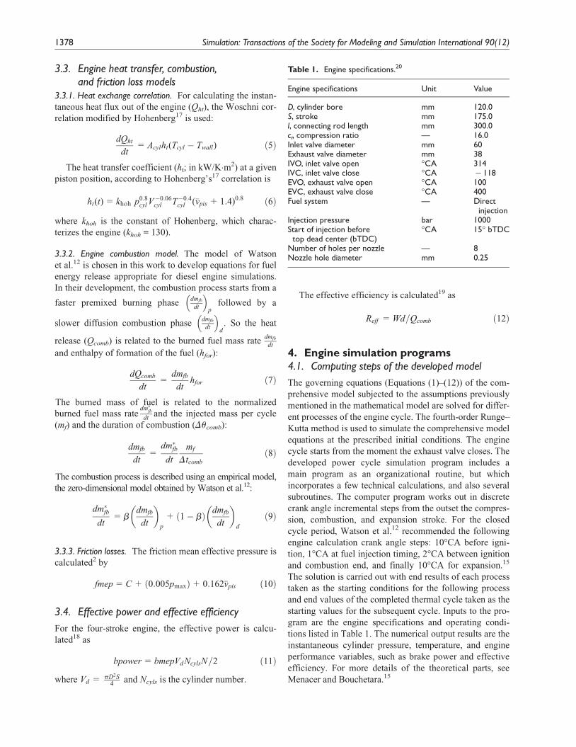
starting values for the subsequent cycle. Inputs to the pro-

gram are the engine specifications and operating condi-

tions listed in Table 1. The numerical output results are the

instantaneous cylinder pressure, temperature, and engine

performance variables, such as brake power and effective

efficiency. For more details of the theoretical parts, see

Menacer and Bouchetara.15

Table 1. Engine specifications.20

Engine specifications Unit Value

D, cylinder bore mm 120.0S, stroke mm 175.0l, connecting rod length mm 300.0cr, compression ratio — 16.0Inlet valve diameter mm 60Exhaust valve diameter mm 38IVO, inlet valve open �CA 314IVC, inlet valve close �CA − 118EVO, exhaust valve open �CA 100EVC, exhaust valve close �CA 400Fuel system — Direct

injectionInjection pressure bar 1000Start of injection beforetop dead center (bTDC)

�CA 15� bTDC

Number of holes per nozzle — 8Nozzle hole diameter mm 0.25


4.2. Commercial engine simulation code

In recent years, a few commercial engine simulation codes,

such as WAVE from Ricardo or GT-Power from Gamma

Technologies, have allowed co-simulations with software

dedicated to control and modeling. Optimized codes and

present computer power make possible detailed engine

simulation within time scales adapted to control system

development. These codes give full phenomenological rep-

resentation of the engine system with one-dimensional

compressible flow formulation. In addition, the code con-

tains several models for heat transfer or combustion.

Diesel engine combustion can be modeled with simple

combustion rate calculation (two functions Wiebe model)

or with a more sophisticated diesel jet model.20 GT-Power

is an object-based code including object libraries for

engine components (pipes, cylinder, cranktrain, compres-

sor, valve, etc.). Building an engine model with GT-Power

consists of parameterization and connection of these

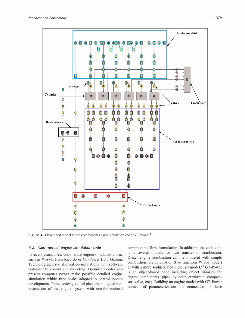
Figure 3. Developed model in the commercial engine simulation code GT-Power.15


objects. Figure 3 shows the developed model in the com-

mercial engine simulation code GT-Power. In the model-

ing view, the line of the exhaust manifold is composed in

three volumes: the cylinders are grouped by three and

emerge on two independent manifolds—these two com-

ponents are considered as open thermodynamic systems

with identical volumes—and the third control volume is

used to ensure the junction with the inlet of the turbine.

The turbocharger consists of an axial compressor con-

nected to a turbine by a shaft; the turbine is driven by

exhaust gas to power the compressor. So more air can be

added into the cylinders, allowing an increasing amount

of fuel to be burned compared to a naturally aspirated

engine.21 The heat exchanger can be assimilated to

an intermediate volume between the compressor and

the intake manifold; it solves a system of differential

equations supplementary identical to the manifold. It

appeared to assimilate the heat exchanger as a nondimen-

sional organ.

5. Results of engine simulation

The thermodynamic and geometric parameters chosen in

this study were as follows:

� engine geometry: compression ratio (cr), cylinder

bore (D), and more particularly the stroke–bore

ratio Rsb =LDÞ

�;

� combustion parameters: injected fuel mass (mf),

crankshaft angle marking the injection timing (Tinj),

and cylinder wall temperature (Twall).

Table 1 shows the main parameters of the chosen direct-

injection diesel engine.15,20

(a) (b)GT-Power

30,0

32,5

35,0

37,5

40,0

42,5

45,0

Max

Eff

icie

ncy

%

Dcyl=120 (mm) Dcyl=130 (mm) Dcyl=140 (mm)

150

175

200

225

250

275M

ax P

ower

(kW

)

Fortran

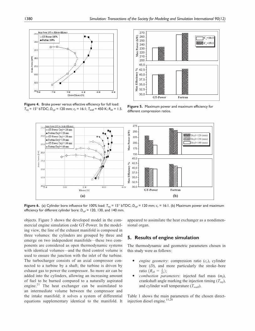
Figure 6. (a) Cylinder bore influence for 100% load: Tinj = 15� bTDC; Dcyl = 120 mm; cr = 16:1. (b) Maximum power and maximumefficiency for different cylinder bore: Dcyl = 120, 130, and 140 mm.

GT-Power Fortran30,032,535,037,540,042,545,0

Max

Eff

ecie

ncy

%

Cr=16:1

Cr=19:1

200210220230240250260270

Max

Pow

er (k

W)

Figure 5. Maximum power and maximum efficiency fordifferent compression ratios.

Figure 4. Brake power versus effective efficiency for full load:Tinj = 15� bTDC; Dcyl = 120 mm; cr = 16:1; Twall = 450 K; Rsb = 1.5.


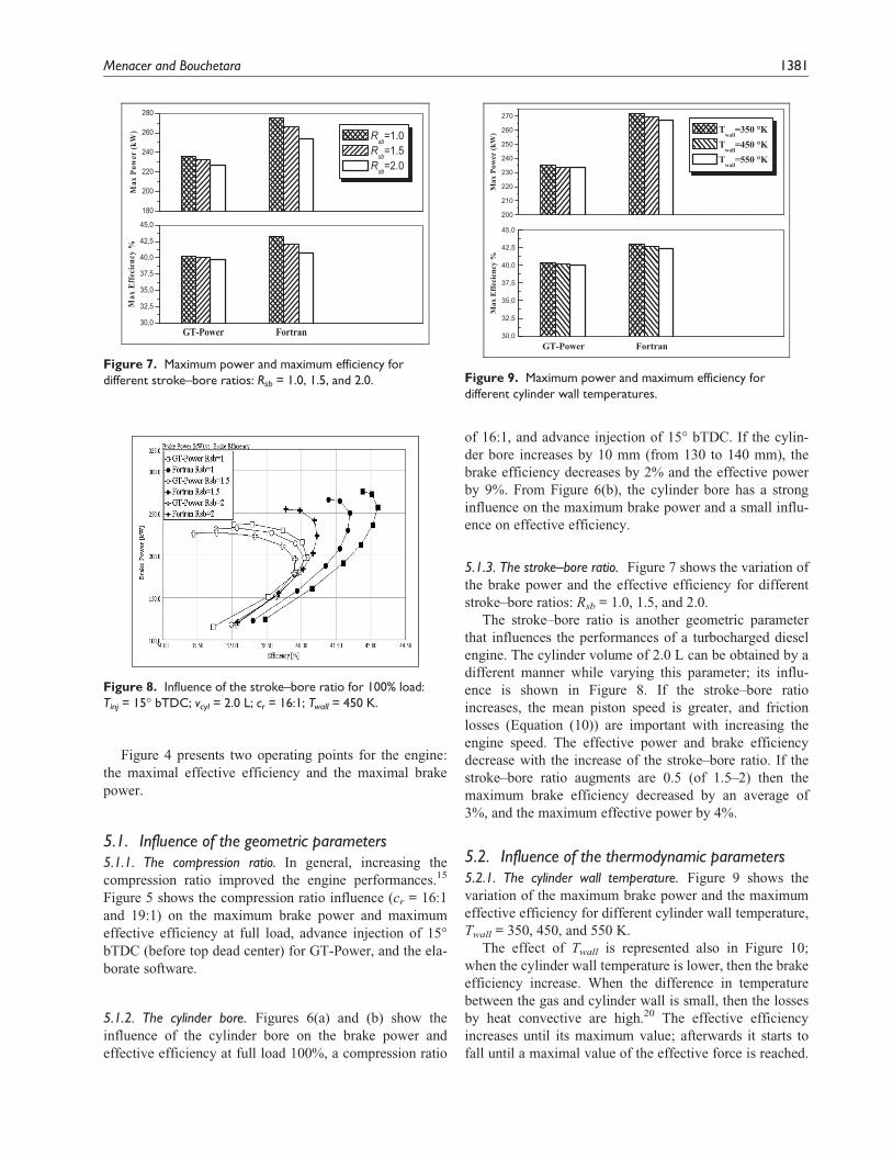
Figure 4 presents two operating points for the engine:

the maximal effective efficiency and the maximal brake

power.

5.1. Influence of the geometric parameters5.1.1. The compression ratio. In general, increasing the

compression ratio improved the engine performances.15

Figure 5 shows the compression ratio influence (cr = 16:1

and 19:1) on the maximum brake power and maximum

effective efficiency at full load, advance injection of 15�bTDC (before top dead center) for GT-Power, and the ela-

borate software.

5.1.2. The cylinder bore. Figures 6(a) and (b) show the

influence of the cylinder bore on the brake power and

effective efficiency at full load 100%, a compression ratio

of 16:1, and advance injection of 15� bTDC. If the cylin-

der bore increases by 10 mm (from 130 to 140 mm), the

brake efficiency decreases by 2% and the effective power

by 9%. From Figure 6(b), the cylinder bore has a strong

influence on the maximum brake power and a small influ-

ence on effective efficiency.

5.1.3. The stroke–bore ratio. Figure 7 shows the variation of

the brake power and the effective efficiency for different

stroke–bore ratios: Rsb = 1.0, 1.5, and 2.0.

The stroke–bore ratio is another geometric parameter

that influences the performances of a turbocharged diesel

engine. The cylinder volume of 2.0 L can be obtained by a

different manner while varying this parameter; its influ-

ence is shown in Figure 8. If the stroke–bore ratio

increases, the mean piston speed is greater, and friction

losses (Equation (10)) are important with increasing the

engine speed. The effective power and brake efficiency

decrease with the increase of the stroke–bore ratio. If the

stroke–bore ratio augments are 0.5 (of 1.5–2) then the

maximum brake efficiency decreased by an average of

3%, and the maximum effective power by 4%.

5.2. Influence of the thermodynamic parameters5.2.1. The cylinder wall temperature. Figure 9 shows the

variation of the maximum brake power and the maximum

effective efficiency for different cylinder wall temperature,

Twall = 350, 450, and 550 K.

The effect of Twall is represented also in Figure 10;

when the cylinder wall temperature is lower, then the brake

efficiency increase. When the difference in temperature

between the gas and cylinder wall is small, then the losses

by heat convective are high.20 The effective efficiency

increases until its maximum value; afterwards it starts to

fall until a maximal value of the effective force is reached.

GT-Power Fortran30,0

32,5

35,0

37,5

40,0

42,5

45,0

Max

Eff

ecie

ncy

%

Twall

=350 °KT

wall=450 °K

Twall

=550 °K

200

210

220

230

240

250

260

270

Max

Pow

er (k

W)

Figure 9. Maximum power and maximum efficiency fordifferent cylinder wall temperatures.


32,5

35,0

37,5

40,0

42,5

45,0

Max

Effe

cien

cy %

Rsb=1.0Rsb=1.5Rsb=2.0

180

200

220

240

260

280

Max

Pow

er (k

W)

Figure 7. Maximum power and maximum efficiency fordifferent stroke–bore ratios: Rsb = 1.0, 1.5, and 2.0.

Figure 8. Influence of the stroke–bore ratio for 100% load:Tinj = 15� bTDC; vcyl = 2.0 L; cr = 16:1; Twall = 450 K.


It is also valid for the effective power. If the cylinder wall

temperature increases by 100 K (from 350 to 450 K), the

maximum brake power and effective efficiency decrease

respectively by about 0.7%. The maximum operating tem-

perature of an engine is limited by the strength and geo-

metric variations due to thermal expansion, which can be a

danger of galling. Improved heat transfer to the walls of

the combustion chamber lowers the temperature and pres-

sure of the gas inside the cylinder, which reduces the work

transferred to the piston cylinder and reduces the thermal

efficiency of the engine. It is thus advantageous to cool the

cylinder walls provided they do not do it too vigorously.

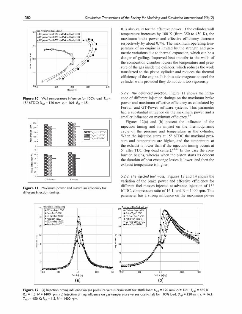
5.2.2. The advanced injection. Figure 11 shows the influ-

ence of different injection timings on the maximum brake

power and maximum effective efficiency as calculated by

Fortran and GT-Power software systems. This parameter

had a substantial influence on the maximum power and a

smaller influence on maximum efficiency.15

Figures 12(a) and (b) present the influence of the

injection timing and its impact on the thermodynamic

cycle of the pressure and temperature in the cylinder.

When the injection starts at 15� bTDC the maximal pres-

sure and temperature are higher, and the temperature at

the exhaust is lower than if the injection timing occurs at

5� after TDC (top dead center).22,23 In this case the com-

bustion begins, whereas when the piston starts its descent

the duration of heat exchange losses is lower, and then the

exhaust temperature is higher.

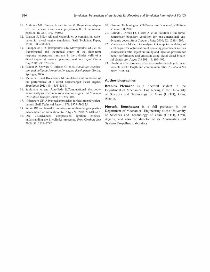
5.2.3. The injected fuel mass. Figures 13 and 14 shows the

variation of the brake power and effective efficiency for

different fuel masses injected at advance injection of 15�bTDC, compression ratio of 16:1, and N = 1400 rpm. This

parameter has a strong influence on the maximum power

Figure 12. (a) Injection timing influence on gas pressure versus crankshaft for 100% load: Dcyl = 120 mm; cr = 16:1; Twall = 450 K;Rsb = 1.5; N = 1400 rpm. (b) Injection timing influence on gas temperature versus crankshaft for 100% load: Dcyl = 120 mm; cr = 16:1;Twall = 450 K; Rsb = 1.5, N = 1400 rpm.

Figure 10. Wall temperature influence for 100% load: Tinj =15� bTDC; Dcyl = 120 mm; cr = 16:1; Rsb =1.5.

GT-Power Fortran15

20

25

30

35

40

45

Max

Eff

icie

ncy

%

Tinj=-15° bTDC Tinj=-5° bTDC Tinj=+5° bTDC

0

50

100

150

200

250

Max

Pow

er (k

W)

Figure 11. Maximum power and maximum efficiency fordifferent injection timings.


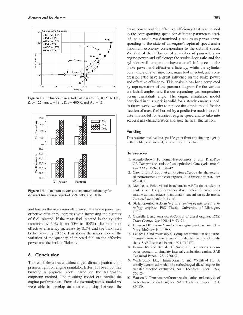
and less on the maximum efficiency. The brake power and

effective efficiency increases with increasing the quantity

of fuel injected. If the mass fuel injected in the cylinder

increases by 50% (from 50% to 100%), the maximum

effective efficiency increases by 3.5% and the maximum

brake power by 28.5%. This shows the importance of the

variation of the quantity of injected fuel on the effective

power and the brake efficiency.

6. Conclusion

This work describes a turbocharged direct-injection com-

pression ignition engine simulator. Effort has been put into

building a physical model based on the filling-and-

emptying method. The resulting model can predict the

engine performances. From the thermodynamic model we

were able to develop an interrelationship between the

brake power and the effective efficiency that was related

to the corresponding speed for different parameters stud-

ied; as a result, we determined a maximum power corre-

sponding to the state of an engine’s optimal speed and a

maximum economy corresponding to the optimal speed.

We studied the influence of a number of parameters on

engine power and efficiency: the stroke–bore ratio and the

cylinder wall temperature have a small influence on the

brake power and effective efficiency, while the cylinder

bore, angle of start injection, mass fuel injected, and com-

pression ratio have a great influence on the brake power

and effective efficiency. This analysis has been completed

by representation of the pressure diagram for the various

crankshaft angles, and the corresponding gas temperature

versus crankshaft angle. The engine simulation model

described in this work is valid for a steady engine speed.

In future work, we aim to replace the simple model for the

fraction of mass fuel burned by a predictive model, to vali-

date this model for transient engine speed and to take into

account gas characteristics and specific heat fluctuation.

Funding

This research received no specific grant from any funding agency

in the public, commercial, or not-for-profit sectors.

References

1. Angulo-Brown F, Fernandez-Betanzos J and Diaz-Pico

CA.Compression ratio of an optimized Otto-cycle model.

Eur J Phys 1994; 15: 38–42.

2. Chen L, Lin J, Lou J, et al. Friction effect on the characteris-

tic performances of diesel engines. Int J Energ Res 2002; 26:

965–971.

3. Merabet A, Feidt M and Bouchoucha A.Effet du transfert de

chaleur sur les performances d’un moteur a combustion

interne atmospherique fonctionnant suivant un cycle mixte.

Termotehnica 2002; 2: 43–46.

4. Stefanopoulou A.Modeling and control of advanced tech-

nology engines. PhD Thesis, University of Michigan,

1996.

5. Guzzella L and Amstutz A.Control of diesel engines. IEEE

Trans Control Syst 1998; 18: 53–71.

6. Heywood JB.Internal combustion engine fundamentals. New

York: McGraw-Hill, 1988.

7. Ledger JD and Walmsley S. Computer simulation of a turbo-

charged diesel engine operating under transient load condi-

tions. SAE Technical Paper, 1971, 710177.

8. Benson RS and Baruah PC. Some further tests on a com-

puter program to simulate internal combustion engine. SAE

Technical Paper, 1973, 730667.

9. Winterborne DE, Thiruarooran C and Wellstead PE. A

wholly dynamical model of a turbocharged diesel engine for

transfer function evaluation. SAE Technical Paper, 1977,

770124.

10. Watson N. Transient performance simulation and analysis of

turbocharged diesel engines. SAE Technical Paper, 1981,

810338.


32,5

35,0

37,5

40,0

42,5

45,0

Max

Effe

cienc

y %

25% 50% 100%

50

100

150

200

250

Max

Pow

er (k

W)

Figure 14. Maximum power and maximum efficiency fordifferent fuel masses injected: 25%, 50%, and 100%.

Figure 13. Influence of injected fuel mass for Tinj = 15� bTDC,Dcyl= 120 mm, cr = 16:1, Twall = 480 K, and βmb =1.5.


11. Anthoine MP, Dauron A and Serine M. Regulation adapta-

tive de richesse avec sonde propotionnelle et actionneur

papillon. In: SIA, 1992, 92032.

12. Watson N, Pilley AD and Marzouk M. A combustion corre-

lation for diesel engine simulation. SAE Technical Paper,

1980, 1980–800029.

13. Rakopoulos CD, Rakopoulos CD, Mavropoulos GC, et al.

Experimental and theoretical study of the short-term

response temperature transients in the cylinder walls of a

diesel engine at various operating conditions. Appl Therm

Eng 2004; 24: 679–702.

14. Gunter P, Schwarz C, Stiesch G, et al. Simulation combus-

tion and pollutant formation for engine-development. Berlin:

Springer, 2006.

15. Menacer B and Bouchetara M.Simulation and prediction of

the performance of a direct turbocharged diesel engine.

Simulation 2013; 89: 1355–1368.

16. Sakhrieha A and Abu-Nada E.Computational thermody-

namic analysis of compression ignition engine. Int Commun

Heat Mass Transfer 2010; 37; 299–303.

17. Hohenberg GF. Advanced approaches for heat transfer calcu-

lations. SAE Technical Paper, 1979, 1979–790825.

18. Semin RB and Ismail R.Investigation of diesel engine perfor-

mance based on simulation. Am J Appl Sci 2008; 5: 610–617.

19. Dec JE.Advanced compression ignition engines-

understanding the in-cylinder processes. Proc Combust Inst

2009; 32: 2727–2742.

20. Gamma Technologies. GT-Power user’s manual, GT-Suite

Version 7.0, 2009.

21. Galindo J, Arnau FJ, Tiseira A, et al. Solution of the turbo-

compressor boundary condition for one-dimensional gas-

dynamic codes. Math Comput Model 2010; 52: 1288–1297.

22. Venkatraman M and Devaradjane G.Computer modeling of

a CI engine for optimization of operating parameters such as

compression ratio, injection timing and injection pressure for

better performance and emission using diesel-diesel biodie-

sel blends. Am J Appl Sci 2011; 8: 897–902.

23. Ebrahimi R.Performance of an irreversible diesel cycle under

variable stroke length and compression ratio. J Ambient Sci

2009; 7: 58–64.

Author biographies

Brahim Menacer is a doctoral student in the

Department of Mechanical Engineering at the University

of Sciences and Technology of Oran (USTO), Oran,

Algeria.

Mostefa Bouchetara is a full professor in the

Department of Mechanical Engineering at the University

of Sciences and Technology of Oran (USTO), Oran,

Algeria, and also the director of its Aeronautics and

Systems Propelling Laboratory.


Documents

Parametric study of the performance of a turbocharged compression