Embed Size (px)
Citation preview

Part 2
By Xiao Qin
1

The crash severity model is to use statistical methods for identifying factors that are significantly associated with the consequence of a traffic crash, and their relationships.
The response variable is the person who sustains the most severe injury in a crash in the KABCO scale (i.e., killed, incapacitating injury, non-incapacitating injury, possible injury, and no injury).
A variety of models have been developed to account for data issues and methodological limitations.
The common modeling approaches include logistic, probit and their variations.
The impact of a factor on the injury severity levels can be estimated through its marginal effect or odds ratio.

Learn the characteristics of crash injury severity data.
Gain the knowledge about data limitations and modeling challenges.
Understand the assumptions, property and limitations of models for crash injury severity levels.
Develop crash injury severity models and perform analysis.
Interpret the modeling results.

Injury severity has a finite number of outcomes that are categorized on the KABCO scale
KABCO scale and AIS scale Imbalanced observations across at different scales Reporting inconsistency and underreporting Non-ordinal or ordered probabilistic if an ordinal structure for the response
variable is assumed; fixed or random parameter models, depending on the assumption for model coefficient estimation
Sample size for injury severity models Utility, utility function and random utility function Probit model and logistic regression model: model assumption, model
estimation and model results interpretation (e.g., probability, odds, odds ratio, marginal effect, elasticity)
Model variations are available if restrictions such as irrelevant and independent alternatives (IIA), proportional odds are relaxed
4

5

Can we increase the bus ridership by painting the bus with a different color?
UWM UWM
6

Clearly, the bus share should not have been changed. What is wrong?
The problem is with the underlying assumption in the logit model. The logit model requires that alternatives be independent (i.e. εred and εblue be independent). This is not the case in this example.
Obviously, the errors of the perceived utility from alternative of the red bus is dependent on the error from the blue bus, and vice versa. This does not justify the use of logit model.
Note: when the alternatives are distinctly different and independent, the logit model shall work well.
7

To overcome the IIA problem, the idea behind a nested logit model is to group alternate outcomes suspected of sharing unobserved effects into nests (this sharing sets up the disturbance term correlation that violates the derivation assumption).
Because the outcome probabilities are determined by differences in the functions determining these probabilities (both observed and unobserved), shared unobserved effects will cancel out in each nest providing that all alternatives in the nest share the same unobserved effects.
8

9

Mathematically, McFadden (1981) has shown the GEV disturbance assumption leads to the following model structure for observation nchoosing outcome i
WherePn(i) is the unconditional probability of observation n having discrete outcome i,'s are vectors of characteristics that determine the probability of discrete outcomes,'s are vectors of estimable parameters, Pn(ji) is the probability of observation n having discrete outcome j conditioned on the outcome being in
outcome category i, J is the conditional set of outcomes (conditioned on i), I is the unconditional set of outcome categories,
LSin is the inclusive value (logsum), and i is an estimable parameter.
(4.8a)
(4.8b)
(4.8c)
10
In order to be consistent with McFadden’s generalized extreme value derivation of the model, the parameter estimate for ϕi in the nested logit model must be between zero and one.
If ϕi equals to one or is not significantly different from one, there is no correlation between the severity levels in the nest, meaning the model reduces to the multinomial logit model.
If ϕi equals to zero, a perfect correlation is implied among the severity levels in the nest, indicating a deterministic process by which crashes result in particular severity levels.
The t test can be used to test if ϕi is significantly different from 1. Because ϕi is less than or equal to one, this is a one-tailed t test (half of the two-tailed t-test).
It is important to note that the typical t-test implemented in many commercial software packages are against zero instead of one. Thus, the t value must be calculated manually. The IIA assumption for a MNL model can also be tested with the Hausman-McFadden (1984) test which has been widely implemented in commercial statistical software.
11

Done in a sequential fashion.◦ Estimate the conditional model using only the
observations in the sample that are observed having discrete outcomes J.
◦ Once these estimation results are obtained, the logsum is calculated (this is the denominator of one or more of the conditional models) for all observations, both those selecting J and those not.
The full information maximum likelihood (FIML) estimation (Greene, W., Econometric Analysis, 2000).
12

Exercise 4.2: Coefficient Estimates for NL*
*: partial results shown here
13

1. Establish the nested structure of crash severities. :
2. Determine the functional form based on Eq. 4.8 (a), (b) and (c). For example, Pn(j|i) is the probability of crash n having injury outcome B or C conditioned on the injury outcome being in category not a K or A injury. I is the unconditional set of outcome categories (for example, the upper three branches in the figure: no K/A injury and K/A injury). LSni is the inclusive value (logsum).
3. Estimate the coefficients using the R “mlogit” package:nested_logit <- mlogit(INJSVR ~ 0|YOUNG + OLD + FEMALE + ALCFLAG + DRUGFLAG + SAFETY + DRVRPC_SPD + DRVRPC_RULEVIO + DRVRPC_RECK + TRFCONT_SIGNAL + TRFCONT_2WAY + TRFCONT_NONE + TOTUNIT + ROADCOND_SNOW + ROADCOND_ICE + ROADCOND_WET + LGTCOND_DARK, data = crash_mnl, nests = list(KA = c("3"), non_KA = c("1", "2")), un.nest.el = TRUE).
4. summarize your findings. The AIC value of the NL model (17871.11) is greater than that of MNL model (17869.32), indicating inferior performance. The inclusive value is 0.7161 and its t-value is -0.474. Apparently, the log-sum coefficient is not significantly different from 1. When the inclusive value is equal to one or not significantly different from 1, there is no correlation between the severity levels in the nest. We can conclude that for this dataset, the MNL model is more appropriate. 14
B, C, or PDO K or A
B or C PDO

◦ More aggregate – cannot include specific accident characteristics (driver characteristics, vehicle characteristics, restraint usage, alcohol consumption, etc.). ◦ Without detailed accident information, the approach
potentially introduces a heterogeneity problem.◦ Heterogeneity could result in varying effects of X that
could be captured with random parameters. ◦ Mixed logit may be appropriate. Relaxes possible IIA problems with a more general error-term structure. Can test a variety of distribution options for β . Estimated with simulation based maximum likelihood.
15

16
Similar to the random parameter model for crash-frequency. This means that the coefficients are allowed to vary across observations.
where 𝑓 𝜷|𝝋 is a density function of 𝜷 and 𝝋 is a vector of parameters which specify the density function, with all other terms as previously defined.
(4.9)
In a statistics term, the weighted average of several functions is called a mixed function, and the density that provides the weights is called the mixing distribution. Mixed logit is a mixture of the standard logit function evaluated at different 𝜷 with f(𝜷) being the mixing distribution.

The injury severity level probability is a mixture of logits. When all parameters β are fixed, the model reduces to the multinomial logit model.
When β is allowed to vary, the model is not in a closed form, and the probability of crash observation n having a particular injury outcome ican be calculated through integration.
Simulation-based maximum likelihood methods such as Halton draws are usually used.
The choice of the density function of β depends on the nature of the coefficient and the statistical goodness of fit. ◦ The lognormal distribution is useful when the coefficient is known to have the same sign for
each observation. ◦ Triangular and uniform distributions have the advantage of being bounded on both sides. ◦ Furthermore, triangular assumes that the probability increases linearly from the beginning to
the mid-range and then decreases linearly to the end. ◦ A uniform distribution assumes the same probability for any value within the range.
17

Random coefficient: 𝑈 𝛽 𝑥 𝜀 where 𝛽 can be decomposed into mean 𝛼 and deviations 𝜇 such as 𝛼 𝑥 𝜇 𝑥 and 𝜀 is a random term that is iidextreme value.
Error components: 𝑈 𝛼 𝑥 𝜇 𝑧 𝜀 where 𝑥 and 𝑧 are vectors of observable variables relating to alternative j. 𝛼 is a vector of fixed parameters and 𝜇 is random with zero mean, and 𝜀 is iid extreme value. So, the random portion of utility is (𝜇 𝑧 𝜀 ) which can be correlated over alternatives depending on 𝑧.
Error-component and random-coefficient specifications are formally equivalent; but a researcher thinks about the model affects the specification of the mixed logit.
It is important to know that the mixing distribution, whether driven by random parameters or by error components, captures variance and correlations in unobserved factors. But there is a limit on how much one can learn about things that are not seen.
18

Exercise 4.3: Coefficient Estimates for ML*
*: partial results shown here
19

1. Determine the density function in the R “mlogit” package, random parameter object “rpar” contains all the relevant information about the distribution of random parameters. Currently, the normal ("n"), log-normal ("ln"), zero-censored normal ("cn"), uniform ("u") and triangular ("t") distributions are available. For illustration, normal distribution is chosen as the density function of random parameter β.
2. Estimate the coefficients using the R “mlogit” package:crash_data_mixed <- mlogit.data(data_mixed_ch4, shape = "long", choice = "INJSVR", chid.var = "ID", alt.var = "OUTCOME")mixed_logit <- mlogit(INJSVR ~ OLD_2 + OLD_3 + FEMALE_2 + FEMALE_3 + ALCFLAG_2 + ALCFLAG_3 + DRVRPC_SPD_2 + DRVRPC_SPD_3 + ROADCOND_SNOW_2 + ROADCOND_SNOW_3 + LGTCOND_DARK_2 + LGTCOND_DARK_3, data = crash_data_mixed, rpar = c(FEMALE_2 = 'n’, FEMALE_3 = 'n', ALCFLAG_3 = 'n', DRVRPC_SPD_3 = 'n', ROADCOND_SNOW_2 = 'n’, ROADCOND_SNOW_3 = 'n', LGTCOND_DARK_3 = 'n'),panel = FALSE, correlation = FALSE, R = 100, halton = NA).
Note: rpar argument names random coefficients (‘n’ for a normal distribution); halton=NA means default haltondraws are applied. (if interested, read “Halton Sequences for Mixed Logit” by Kenneth Train at https://eml.berkeley.edu/wp/train0899.pdf)
3. Summarize the findings. The ML model can account for the data heterogeneity by treating coefficients as random variables. the snowy surface parameter for truck K or A injuries is fixed (-10.830); and for severity B or C, it is normally distributed with a mean of -0.8892 and a standard deviation of 1.8159, meaning that 31% of truck crashes occurring on snowy pavement have an increased possibility of B or C injuries. It is plausible that people often drive more slowly and cautiously on snowy roads but that the slick conditions still have a tendency to cause accidents.
20

In Milton et al. (2008), the application of the mixed logit model (also called the random parameters logit model) is undertaken by considering injury-severity proportions for individual roadway segments.
For all of the random parameters, the normal distribution was found to provide the best statistical fit (among normal, lognormal, triangular and uniform).
21
“the constant for the property-damage only proportion is normally distributed with mean −0.355 and standard deviation 1.776. ….This variability is likely capturing the unobserved heterogeneity in the roadway segments that could include factorssuch as visual noise and other physical and environmental factors. ….The average daily traffic (ADT) per lane is normally distributed with a mean 0.0403 and standard deviation 0.515. … 46.9% of the distribution is less than 0 and 53.1% is greater than 0…. a complex interaction among traffic volume, driver behavior and accident-injury severity.”
Milton, J. C., Shankar, V. N., & Mannering, F. L. (2008). Highway accident severities and the mixed logit model: an exploratory empirical analysis. Accident Analysis & Prevention, 40(1), 260-266.

In Milton et al. (2008), the application of the mixed logit model (also called the random parameters logit model) is undertaken by considering injury-severity proportions for individual roadway segments.
22
“The percentage of trucks…had a mean of−0.129 and standard deviation 0.1143, being less than 0 for 87.1% of the roadway segments and greater than 0 for 12.9% of the segments…in a small proportion of roadway segments, the truck percentage increases the proportion of possible injury accidents, while in a majority of roadway segments, the proportion tends to decrease. Note that this variable implies that for 87.1% of roadway segments increasing truck percentages make the severity proportions more likely to be minor (property damage only) or major (injury)... 75.2% of the roadway segments negative values (an increasing number of trucks decreases the likelihood of accidents resulting in injury) and 24.8% positivevalues (an increasing number of trucks increases the likelihood of accidents resulting in injury).The net effect of these twotruck variables points to a fairly complex picture of the effect of trucks on accident-injury severities.”

23

The primary rationale for using ordered discrete choice models for modeling crash severity is that there is an intrinsic order among injury severities, with fatality being the highest order and property damage being the lowest. Including the ordinal nature of the data in the statistical model defends the data integrity and preserves the information.
Second, the consideration of ordered response models avoids the undesirable properties of the multinomial model such as the IIA in the case of a multinomial logit model or a lack of closed-form likelihood in the case of a multinomial probit model.
Third, ignoring the ordinality of the variable may cause a lack of efficiency (i.e., more parameters may be estimated than are necessary if the order is ignored).
Although there are many positives to the ordered model, the disadvantage is that imposing restrictions on the data may not be appropriate despite the appearance of a rank. Therefore, it is important to test the validity of the ordered restriction.
24

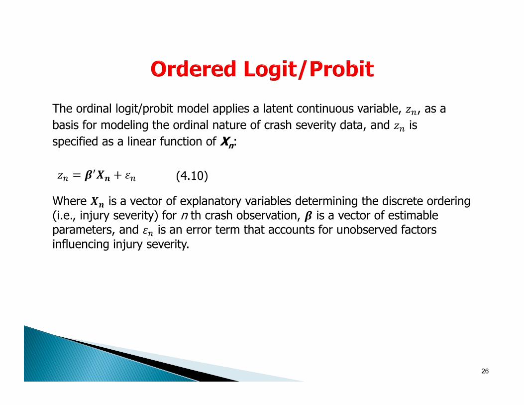
Ordered probability models are derived by defining an unobserved variable Z that is used as a basis for modeling the ordinal ranking of data.
Observed ordinal data, y, for each observation are defined as, A high indexing of zn is expected to result in a high level of observed injury
yn in the case of a crash. The observed discrete injury severity variable yn is stratified by thresholds as follows:
25
1
1 2
2 3
3 4
4
1, PDO or no injury
2, injury C
3, injury B
4, injury A
5, K or fatal injury
n
n
n n
n
n
if z
if z
y if z
if z
if z
(4.11)
Where 's are estimable parameters (referred to as thresholds) that define y, and y corresponds to integer ordering, and I is the highest integer ordered response.
26
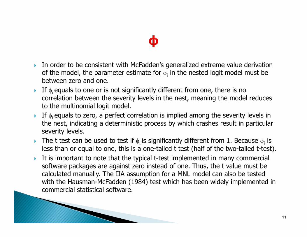
The ordinal logit/probit model applies a latent continuous variable, 𝑧 , as a basis for modeling the ordinal nature of crash severity data, and 𝑧 is specified as a linear function of Xn:
𝑧 𝜷 𝑿𝒏 𝜀
Where 𝑿𝒏 is a vector of explanatory variables determining the discrete ordering (i.e., injury severity) for n th crash observation, 𝜷 is a vector of estimable parameters, and 𝜀 is an error term that accounts for unobserved factors influencing injury severity.
(4.10)

is assumed to be normally distributed across observations with N(0,1), resulting in an ordered probit model
(4.12)
27
1 1 1
1
1 Pr 1 Pr Pr Prn n n n n n n
n
P y z
x β x β
x β
1 2 1 1
2 1
2 1
2 Pr 2 Pr Pr
Pr Prn n n n n
n n n n
n n
P y z
x β
x β x β
x β x β 11n i n i nP i x β x β
𝑃 𝐼 𝑃𝑟 𝑦 𝐼 𝑃𝑟 𝑧 𝜇 1 𝛷 𝜇 𝒙 𝜷

If is assumed to be normally distributed across observations with N(0,1), an ordered probit model results with the ordered selection probabilities being
Note threshold 𝜇 is set equal to 0 without loss of generality (this implies that one need only estimate I-2 thresholds.
28
𝜇 =0

The difficulty arises because the areas between the shifted thresholds may yield increasing or decreasing probabilities after shifts to the left or right, especially for the intermediate categories (i.e., y=2, y=3, and y=4).
The change depends on the location of the thresholds.
A trade-off is inherently being made between recognizing the ordering of responses and losing the flexibility in specification offered by unordered probability models.
29
?? ?

𝑃 𝑢 𝑖 Φ 𝜇 𝛽𝑋 Φ 𝜇 𝛽𝑋Where 𝜇 and 𝜇 represent the upper and lower thresholds for outcome i. The likelihood function is:
𝐿 𝑢 𝛽, 𝜇 Φ 𝜇 𝛽𝑋 Φ 𝜇 𝛽𝑋
𝐿𝐿 𝑢 𝛽, 𝜇 𝛿 𝐿𝑁 Φ 𝜇 𝛽𝑋 Φ 𝜇 𝛽𝑋
where 𝛿 1 if the observed discrete outcome for observation n is i, and zero otherwise. Maximize the LL is subject to the constraint 0≤1 ≤2… ≤I-2
30

Ordered logit can also be conceptualized as a latent variable model.
Let Z be a continuous random variable that depends on a set of explanatory variables X, Z = X + , that is used as a basis for modeling the ordinal ranking of data.
If we assume that follows a standard logistic distribution, it follows the cumulative logit, also known as ordered or ordinal logit model.
31
Recall 4.11,
32
1
1 2
2 3
3 4
4
1, PDO or no injury
2, injury C
3, injury B
4, injury A
5, K or fatal injury
n
n
n n
n
n
if z
if z
y if z
if z
if z
Pr Pr Pr
exp11 exp 1 exp
n n i n i n
n i
i n n i
y i Z
x β
x βx β x β
(4.15)
exp1 exp
nn
n
F
Where εn follows logistic distribution whose CDF is:
𝑃𝑟 𝜀 𝜇 𝒙 𝜷 1 𝐹 𝜀𝒙 𝜷
.So,
Model can be specified as below𝑙𝑜𝑔 𝒙𝒏𝜷 𝜇 i=1, …, I-1 (4.13)

The fact that you can calculate odds ratios highlights a key assumption of ordered logit: “Proportional odds assumption” Also known as the “parallel regression assumption” Which also applies to ordered probit
Model assumes that variable effects on the odds of lower vs. higher outcomes are consistent; or regression parameters have to be the same for different response outcomes.
If this assumption doesn’t seem reasonable, consider multinomial logit, generalized ordered logistic and proportional odds model.
33

Consider a model of three injury levels - no injury, injury, and fatality. Suppose that one of the factors is airbag. A negative parameter of the airbag indicator (1 if it was deployed and zero otherwise) becomes greater and hence, shifts values to the right on the X-axle. Thus, the model constrains the effect of the seatbelt to simultaneously decrease the probability of a fatality and increase the no injury probability. But we know for a fact that the activation of an airbag may cause injury and/or decrease no injury; but unfortunately, ordered models cannot account for this bi-directional possibility because the shift in thresholds is constrained to move in the same direction.
34

Exercise 4.4: Coefficient Estimates for OP and OL*
*: partial results shown here
3535
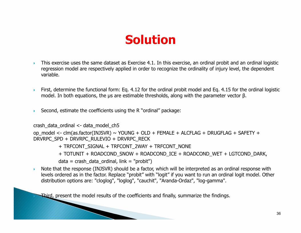
This exercise uses the same dataset as Exercise 4.1. In this exercise, an ordinal probit and an ordinal logistic regression model are respectively applied in order to recognize the ordinality of injury level, the dependent variable.
First, determine the functional form: Eq. 4.12 for the ordinal probit model and Eq. 4.15 for the ordinal logistic model. In both equations, the µs are estimable thresholds, along with the parameter vector β.
Second, estimate the coefficients using the R “ordinal” package:
crash_data_ordinal <- data_model_ch5op_model <- clm(as.factor(INJSVR) ~ YOUNG + OLD + FEMALE + ALCFLAG + DRUGFLAG + SAFETY + DRVRPC_SPD + DRVRPC_RULEVIO + DRVRPC_RECK
+ TRFCONT_SIGNAL + TRFCONT_2WAY + TRFCONT_NONE+ TOTUNIT + ROADCOND_SNOW + ROADCOND_ICE + ROADCOND_WET + LGTCOND_DARK,data = crash_data_ordinal, link = "probit")
Note that the response (INJSVR) should be a factor, which will be interpreted as an ordinal response with levels ordered as in the factor. Replace “probit” with “logit” if you want to run an ordinal logit model. Other distribution options are: "cloglog", "loglog", "cauchit", "Aranda-Ordaz", "log-gamma".
Third, present the model results of the coefficients and finally, summarize the findings.
36

A generalized ordered logistic model (gologit) provides results similar to those that result from running a series of binary logistic regressions/ cumulative logit models.
The ordered logit model is a special case of the gologit model where the coefficients β are the same for each category.
A gologit model and an MNL model, whose variables are freed from the proportional odds constraint, both generate many more parameters than an ordered logit model.
The partial proportional odds model (PPO) is in between, as some of the coefficients β are the same for all categories and others may differ.
A PPO model allows for the parallel lines/ proportional odds assumption to be relaxed for those variables that violate the assumption.
37

𝑃𝑟 𝑦𝑛 𝑖𝑒𝑥𝑝 𝐱𝑛′ 𝛃𝒊 𝜇𝑖
1 𝑒𝑥𝑝 𝐱𝑛′ 𝛃𝒊 𝜇𝑖, 𝑖 1, … 𝐼 1
In the gologit model, the probability of crash injury for a given crash can be specified as (I-1) set of equations:
Where μi is the cut-off point for the ith cumulative logit. Note that Equation 4.16 is different from Equation 4.14 in that βi is a single set of coefficients that vary by category i.
38
(4.16)

In the PPO model formulation, it is assumed that some explanatory variables may satisfy the proportional odds assumption while some may not. The cumulative probabilities in the PPO model are calculated as follows:
Where xn is a (p×1) vector of independent variables of crash n, β is a vector of regression coefficients, and each independent variable has a β coefficient. Tn is a (q×1) vector (q≤p) containing the values of crash n on the subset of p explanatory variables for which the proportional odds assumption is not assumed, and γi is a (q×1) vector of regression coefficients. So, γi represents deviation from the proportionality βi and is an increment associated only with the ithcumulative logit, i=1,⋯,(I-1).
39
𝑃𝑟 𝑦 𝑖 𝒙 𝜷 𝑻 𝜸𝒊𝒙 𝜷 𝑻 𝜸𝒊
, 𝑖 1, … 𝐼 1 (4.17)

An alternative but simplified way to think about the PPO model is to have two sets of explanatory variables: x1, the coefficients of which remain the same for all injury severities and x2, the coefficients of which vary across injury severities.
40
1 1 2 2
1 1 2 2
expPr
1 expi i
ni i
y i
x β x βx β x β
(4.18)

Although the generalized ordered logit model relaxes the proportional odds assumption by allowing some or all of the parameters to vary by severity levels, the set of explanatory variables is invariant over all severity levels.
The sequential logit/probit regression model should be considered when the difference in the set of explanatory variables at each severity level is important.
Sequential logit/probit regression allows different regression parameters for different severity levels. A sequential logit/probit model supposes (I-1) latent variables given as (I-1) sets of equations.
Sequential logistic regression not only accounts for the inherent order of dependent variables but also allows different sets of regression parameters to be independently considered in the model specification.
41

42
where zni is a continuous latent variable that determines whether the injury severity is observed as i or higher, βi’s are the vectors of estimated parameters, and εni’s are error terms that are independent of xn.
(4.19)

The sequential model is a type of hierarchical model where lower stages mean lower injury severity.
For example, stage 1 of the KABCO scale may be KABC versus O; stage 2 may be KAB versus C and stage 3 may be KA versus B. This change in definition matters when explaining the model results. Moreover, the hierarchical structure can be arranged from low to high or from high to low, which can also be called “forward” or “backward.”
It is important to know that the sequential model uses a subpopulation of the data to estimate the variant set of βi. The subpopulation decreases as the stages progresses forward or backward. In the forward format, all data are used in the first stage to estimate β1, but only the crashes with injury type C or higher are used in the second stage to estimate β2. Crashes with injury type B or higher are used in the second stage to estimate β3.
43

Jung et al. (2010) applied the sequential logit model to assess the effects of rainfall on the severity of single-vehicle crashes on Wisconsin interstate highways. ◦ The sequential logit regression model outperformed the ordinal logit
regression model in predicting crash severity levels in rainy weather when comparing goodness of fit, parameter significance, and prediction accuracies.
◦ The sequential logit model identified that stronger rainfall intensity significantly increases the likelihood of fatal and incapacitating injury crash severity, while this was not captured in the ordered logit model.
Yamamoto et al. (2008) also reported superior performance and unbiased parameter estimates with sequential binary models as compared with traditional ordered probit models, even when underreporting was a concern.
44

Where P1=probability of PDO;P2=probability of possible injury; and P3 = probability of fatal/incapacitating/non-incapacitating injury
DCD is defined as the minimum safe stopping distance (SSD) OCC: Average 5-min OCC (%)
Stage 1
Stage 2
Stage 1
Stage 2
Reference: Soyoung Jung, Xiao Qin, David Noyce (2012). Injury Severity of Multi-Vehicle Crash in Rainy Weather, ASCE, Journal of Transportation Engineering, 138(1), pp. 1-12.
45

To properly interpret model results, we need to be wary of the data formats as they can be structured differently because of different methods.
The dependent variable can be treated as individual categories, categories higher than level i, or categories lower than level i.
Independent variables can be continuous, indicator (1 or 0) or categorical.
Categorical variables should be converted to dummy variables, with a dummy variable assigned to each distinct value of the original categories.
The coefficient of a dummy variable can be interpreted as the log-odds for that particular value of dummy minus the log-odds for the base value which is 0 (e.g., the odds of being injured when drinking and driving is 10 times of someone who is sober).
46

The key concepts of marginal effect and elasticity are fundamental to understanding model estimates. The marginal effect is the unit-level change in y for a single-unit increase in x if x is a continuous variable.
In a simple linear regression, the regression coefficient of x is the marginal effect, .
Due to the nonlinear feature of logit models, the marginal effect of any continuous independent variable is: .
Such marginal effects are called instantaneous rates of change because they are computed for a variable while holding all other variables as constant.
47
kk
yx
1iki ii
ki
p p px

Elasticity can be used to measure the magnitude of the impact of specific variables on the injury-outcome probabilities.
For a continuous variable, elasticity is the % change in y given a 1% increase in x. It is computed from the partial derivative with respect to the continuous variable of each observation n.
For indicator or dummy variables (those variables taking on values of 0 or 1), a pseudo elasticity of an indicator variable with respect to an injury severity category represents the percent change in the probability of that injury severity category when the variable is changed from zero to one.
48

1. Brant, R., 1990. Assessing proportionality in the proportional odds model for ordinal logistic regression. Biometrics, 46, 1171–1178. doi:10.2307/2532457.
2. Chen, F., S. Chen, 2011, Injury severities of truck drivers in single- and multi-vehicle accidents on rural highways, Accident Analysis and Prevention, vol. 43, no. 5, 1677-1688.
3. Christensen, R. H. B. 2018. Cumulative link models for ordinal regression with the R package Ordinal. Submitted in J. Stat. Software.
4. Greene, W. 2000. Econometric Analysis, 4th Edition, Prentice Hall, Upper Saddle River, NJ.
5. Greene, W. H., and D. A. Hensher. Modeling ordered choices: A primer. Cambridge University Press, 2010.
6. Gumbel, E.J. (1958) Statistics of Extremes, Columbia University Press, New York.
7. Hausman, J.A. and D. McFadden (1984), A Specification Test for the Multinomial Logit Model, Econometrica, 52, pp.1219–1240.
8. Jung, S. Y., X. Qin, and D. A. Noyce. Rainfall effect on single-vehicle crash severities using polychotomous response models. Accident Analysis and Prevention, Vol. 42, No. 1, 2010, pp. 213-224.
9. McCullagh, P. (1980). Regression models for ordinal data. Journal of the Royal Statistical Society: Series B (Methodological), 42(2), 109-127.
10. McFadden, D. (1981) Econometric Models of Probabilistic Choice. In: Manski, C. and McFadden, D., Eds., Structural Analysis of Discrete Data with Econometric Applications, MIT Press, Cambridge, 198-272.
11. McFadden, D., & Train, K. (2000). Mixed MNL models for discrete response. Journal of applied Econometrics, 15(5), 447-470.
12. Milton, J. C., V. N. Shankar, and F. Mannering. Highway accident severities and the mixed logit model: An exploratory empirical analysis. Accident Analysis and Prevention, Vol. 40, No. 1, 2008, pp. 260-266.
13. Mujalli, R. O., López, G., & Garach, L. (2016). Bayes classifiers for imbalanced traffic accidents datasets. Accident Analysis & Prevention, 88, 37-51.
14. Peterson, B., and F. E. Harrell Jr. Partial proportional odds models for ordinal response variables. Applied statistics, 1990, pp. 205-217.
15. Qin, X., Wang, K., & Cutler, C. E. (2013). Analysis of crash severity based on vehicle damage and occupant injuries. Transportation research record, 2386(1), 95-102.
16. Qin, X., Wang, K., & Cutler, C. E. (2013). Logistic regression models of the safety of large
17. trucks. Transportation research record, 2392(1), 1-10.
18. Savolainen, P. T., F. Mannering, D. Lord, and M. A. Quddus. The statistical analysis of highway crash-injury severities: A review and assessment of methodological alternatives. Accident Analysis and Prevention, Vol. 43, No. 5, 2011, pp. 1666-1676.
19. Savolainen, P., and F. Mannering. Probabilistic models of motorcyclists' injury severities in single- and multi-vehicle crashes. Accident Analysis and Prevention, Vol. 39, No. 5, 2007, pp. 955-963.
20. Shankar, V., F. Mannering, and W. Barfield. Statistical analysis of accident severity on rural freeways. Accident Analysis and Prevention, Vol. 28, No. 3, 1996, pp. 391-401.
21. Train, K. Discrete choice methods with simulation (Second Edition). Cambridge university press, 2009.
22. Wang, X. S., and M. Abdel-Aty. Analysis of left-turn crash injury severity by conflicting pattern using partial proportional odds models. Accident Analysis and Prevention, Vol. 40, No. 5, 2008, pp. 1674-1682.
23. Washington, S. P., Karlaftis, M. G., & Mannering, F. (2020). Statistical and econometric methods for transportation data analysis. 3rd Edition, Chapman and Hall/CRC.
24. Williams (2016) Understanding and interpreting generalized ordered logit models, The Journal of Mathematical Sociology, 40:1, 7-20, DOI: 10.1080/0022250X.2015.1112384.
25. Williams, R. Generalized ordered logit/partial proportional adds models for ordinal dependent variables. The Stata Journal, vol. 6, no.1, 2006, pp.58-82.).
26. Yamamoto, T., Hashiji, Junpei, Shankar, V., (2008). “Underreporting in traffic accident data, bias in parameters and the structure of injury severity models”, Accident Analysis Prevention 40, 1320–1329.
27. Yasmin, S., and N. Eluru. Evaluating alternate discrete outcome frameworks for modeling crash injury severity. Accident Analysis and Prevention, Vol. 59, 2013, pp. 506-521.
49