Part 2: Projection and Regression 2-1/45 Econometrics I Professor William Greene Stern School of Business Department of Economics

Part 2: Projection and Regression2-1/45

Econometrics IProfessor William GreeneStern School of Business

Department of Economics


Econometrics I

Part 2 – Projection and Regression


Statistical Relationship

Objective: Characterize the ‘relationship’ between a variable of interest and a set of 'related' variables

Context: An inverse demand equation, P = + Q + Y, Y = income. P and Q are

two obviously related random variables. We are interested in studying the relationship between P and Q.

By ‘relationship’ we mean (usually) covariation. (Cause and effect is problematic.)


Bivariate Distribution - Model for a Relationship Between Two Variables

We might posit a bivariate distribution for P and Q, f(P,Q) How does variation in P arise?

With variation in Q, and Random variation in its distribution.

There exists a conditional distribution f(P|Q) and a conditional mean function, E[P|Q]. Variation in P arises because of Variation in the conditional mean, Variation around the conditional mean, (Possibly) variation in a covariate, Y which shifts the

conditional distribution


Conditional Moments The conditional mean function is the regression

function. P = E[P|Q] + (P - E[P|Q]) = E[P|Q] + E[|Q] = 0 = E[]. Proof: (The Law of iterated

expectations)

Variance of the conditional random variable = conditional variance, or the scedastic function.

A “trivial relationship” may be written as P = h(Q) + , where the random variable = P-h(Q) has zero mean by construction. Looks like a regression “model” of sorts.

An extension: Can we carry Y as a parameter in the bivariate distribution? Examine E[P|Q,Y]


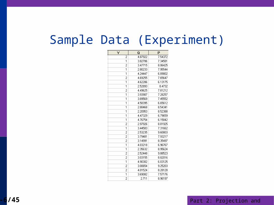
Sample Data (Experiment)


50 Observations on P and QShowing Variation of P Around E[P]


Variation Around E[P|Q](Conditioning Reduces Variation)


Means of P for Given Group Means of Q


Another Conditioning Variable


Conditional Mean Functions

No requirement that they be "linear" (we will discuss what we mean by linear)

Conditional Mean function: h(X) is the function that minimizes EX,Y[Y – h(X)]2

No restrictions on conditional variances at this point.


Projections and Regressions We explore the difference between the linear projection and

the conditional mean function y and x are two random variables that have a bivariate

distribution, f(x,y). Suppose there exists a linear function such that y = + x + where E(|x) = 0 => Cov(x,) = 0 Then, Cov(x,y) = Cov(x,) + Cov(x,x) + Cov(x,) = 0 + Var(x) + 0 so, = Cov(x,y) / Var(x) and E(y) = + E(x) + E() = + E(x) + 0 so, = E[y] - E[x].


Regression and Projection

Does this mean E[y|x] = + x? No. This is the linear projection of y on x It is true in every bivariate distribution,

whether or not E[y|x] is linear in x. y can always be written y = + x + where x, = Cov(x,y) / Var(x) etc. The conditional mean function is h(x) such that y = h(x) + v where E[v|h(x)] = 0. But, h(x)

does not have to be linear.The implication: What is the result of “linearly

regressing y on ,” for example using least squares?


Data from a Bivariate Population


The Linear Projection Computed by Least Squares


Linear Least Squares Projection

----------------------------------------------------------------------Ordinary least squares regression ............LHS=Y Mean = 1.21632 Standard deviation = .37592 Number of observs. = 100Model size Parameters = 2 Degrees of freedom = 98Residuals Sum of squares = 9.95949 Standard error of e = .31879Fit R-squared = .28812 Adjusted R-squared = .28086--------+-------------------------------------------------------------Variable| Coefficient Standard Error t-ratio P[|T|>t] Mean of X--------+-------------------------------------------------------------Constant| .83368*** .06861 12.150 .0000 X| .24591*** .03905 6.298 .0000 1.55603--------+-------------------------------------------------------------


The True Conditional Mean Function

True Conditional Mean Function E[y|x]

X

.35

.70

1.05

1.40

1.75

.00

1 2 30

EXPECTDY


The True Data Generating Mechanism

What does least squares “estimate?”




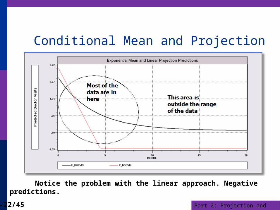
Application: Doctor Visits German Individual Health Care data: N=27,236 Model for number of visits to the doctor:

True E[V|Income] = exp(1.412 - .0745*income) Linear regression: g*(Income)=3.917 - .208*income


Conditional Mean and Projection

Notice the problem with the linear approach. Negative predictions.


Representing the Relationship Conditional mean function: E[y | x] = g(x) Linear approximation to the conditional mean function:

Linear Taylor series evaluated at x0

The linear projection (linear regression?) k

0 K 0 0k=1 k k k

K 00 k=1 k k

g( ) =g( )+Σ [g | = ](x -x )

= +Σ (x -x )

x x x x

Kk k0 1 k k

0

-1

g*(x)= (x -E[x ])

E[y]

Var[ ]} {Cov[ ,y]}x x


Representations of Y


Summary

Regression function: E[y|x] = g(x)

Projection: g*(y|x) = a + bx whereb = Cov(x,y)/Var(x) and a = E[y]-bE[x]Projection will equal E[y|x] if E[y|x] is linear.

Taylor Series Approximation to g(x)


The Classical Linear Regression Model The model is y = f(x1,x2,…,xK,1,2,…K) +

= a multiple regression model (as opposed to multivariate). Emphasis on the “multiple” aspect of multiple regression. Important examples: Marginal cost in a multiple output setting Separate age and education effects in an earnings equation.

Form of the model – E[y|x] = a linear function of x. (Regressand vs. regressors) ‘Dependent’ and ‘independent’ variables.

Independent of what? Think in terms of autonomous variation. Can y just ‘change?’ What ‘causes’ the change? Very careful on the issue of causality. Cause vs. association.

Modeling causality in econometrics…


Model Assumptions: Generalities Linearity means linear in the parameters. We’ll return to

this issue shortly. Identifiability. It is not possible in the context of the

model for two different sets of parameters to produce the same value of E[y|x] for all x vectors. (It is possible for some x.)

Conditional expected value of the deviation of an observation from the conditional mean function is zero

Form of the variance of the random variable around the conditional mean is specified

Nature of the process by which x is observed is not specified. The assumptions are conditioned on the observed x.

Assumptions about a specific probability distribution to be made later.


Linearity of the Model f(x1,x2,…,xK,1,2,…K) = x11 + x22 + … + xKK

Notation: x11 + x22 + … + xKK = x. Boldface letter indicates a column vector. “x” denotes a

variable, a function of a variable, or a function of a set of variables.

There are K “variables” on the right hand side of the conditional mean “function.”

The first “variable” is usually a constant term. (Wisdom: Models should have a constant term unless the theory says they should not.)

E[y|x] = 1*1 + 2*x2 + … + K*xK. (1*1 = the intercept term).


Linearity Simple linear model, E[y|x]=x’β Quadratic model: E[y|x]= α + β1x + β2x2

Loglinear model, E[lny|lnx]= α + Σk lnxkβk

Semilog, E[y|x]= α + Σk lnxkβk

Translog: E[lny|lnx]= α + Σk lnxkβk

+ (1/2) Σk Σl δkl lnxk lnxl

All are “linear.” An infinite number of variations.


Linearity Linearity means linear in the parameters,

not in the variables E[y|x] = 1 f1(…) + 2 f2(…) + … + K fK(…).

fk() may be any function of data. Examples:

Logs and levels in economics Time trends, and time trends in loglinear models –

rates of growth Dummy variables Quadratics, power functions, log-quadratic, trig

functions, interactions and so on.


Uniqueness of the Conditional Mean

The conditional mean relationship must hold for any set of N observations, i = 1,…,N. Assume, that N K (justified later)

E[y1|x] = x1 E[y2|x] = x2 … E[yN|x] = xN All n observations at once: E[y|X] = X = E.


Uniqueness of E[y|X]

Now, suppose there is a that produces the same expected value,

E[y|X] = X = E.

Let = - . Then, X = X - X = E - E = 0.

Is this possible? X is an NK matrix (N rows, K columns). What does X = 0 mean? We assume this is not possible. This is the ‘full rank’ assumption – it is an ‘identifiability’ assumption. Ultimately, it will imply that we can ‘estimate’ . (We have yet to develop this.) This requires N K .


Linear Dependence Example: from your text: x = [1 , Nonlabor income, Labor income, Total income] More formal statement of the uniqueness condition: No linear dependencies: No variable xk may be written

as a linear function of the other variables in the model. An identification condition. Theory does not rule it out, but it makes estimation impossible. E.g.,y = 1 + 2NI + 3S + 4T + , where T = NI+S. y = 1 + (2+a)NI + (3+a)S + (4-a)T + for any a,

= 1 + 2NI + 3S + 4T + . What do we estimate if we ‘regress’ y on (1,NI,S,T)? Note, the model does not rule out nonlinear

dependence. Having x and x2 in the same equation is no problem.


An Enduring Art Mystery

Why do larger paintings command higher prices?

The Persistence of Memory. Salvador Dali, 1931

The Persistence of EconometricsGreene, 2011

Graphics show relative sizes of the two works.

3/49


An Unidentified (But Valid)Theory of Art Appreciation

Enhanced Monet Area Effect Model: Height and Width Effects

Log(Price) = α + β1 log Area +

β2 log Aspect Ratio +

β3 log Height +

β4 Signature +

ε

(Aspect Ratio = Height/Width). This is a perfectly respectable theory of art prices. However, it is not possible to learn about the parameters from data on prices, areas, aspect ratios, heights and signatures.


NotationDefine column vectors of n observations on y and the K

variables.

1 11 12 1 11

2 21 22 2 22

N1 N2 NK

y

K

K

N NK

y x x x

y x x x

y x x x= X +

The assumption means that the rank of the matrix X is K.No linear dependencies => FULL COLUMN RANK of the matrix X.


Expected Values of Deviations from the Conditional Mean

Observed y will equal E[y|x] + random variation. y = E[y|x] + (disturbance)

Is there any information about in x? That is, does movement in x provide useful information about movement in ? If so, then we have not fully specified the conditional mean, and this function we are calling ‘E[y|x]’ is not the conditional mean (regression)

There may be information about in other variables. But, not in x. If E[|x] 0 then it follows that Cov[,x] 0. This violates the (as yet still not fully defined) ‘independence’ assumption


Zero Conditional Mean of ε

E[|all data in X] = 0

E[|X] = 0 is stronger than E[i | xi] = 0 The second says that knowledge of xi provides no

information about the mean of i. The first says that no xj provides information about the expected value of i, not the ith observation and not any other observation either.

“No information” is the same as no correlation. Proof: Cov[X,] = Cov[X,E[|X]] = 0


The Difference Between E[ε |X]=0 and E[ε]=0


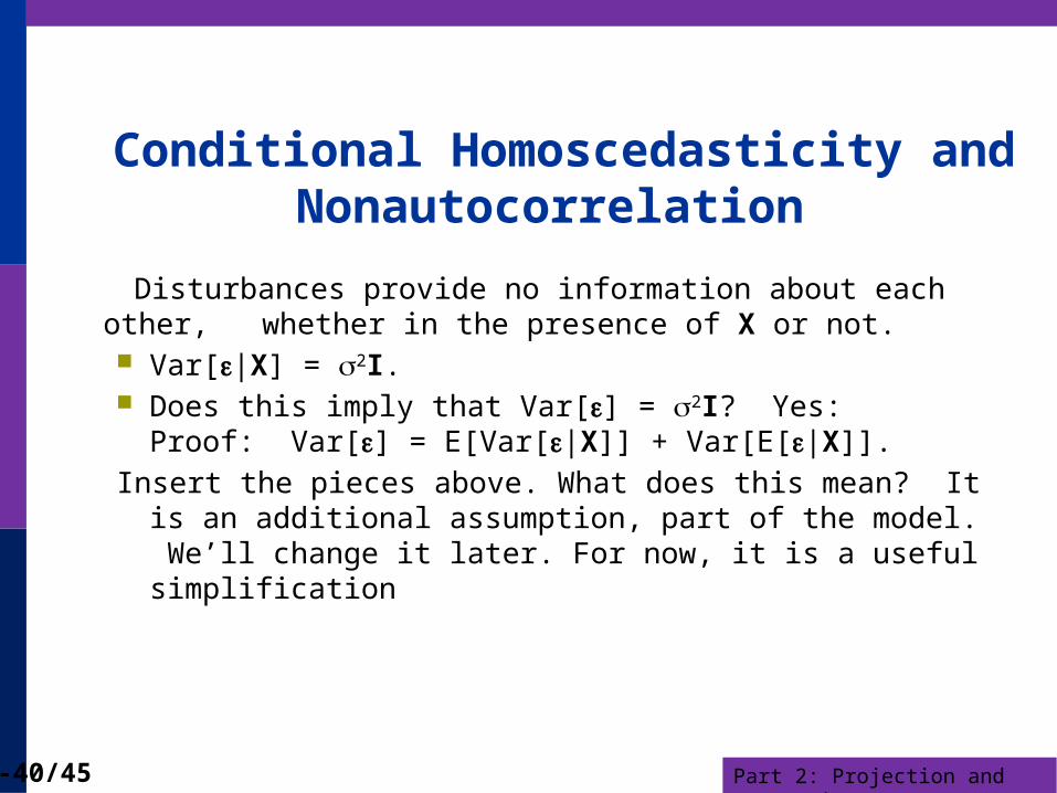
Conditional Homoscedasticity and Nonautocorrelation

Disturbances provide no information about each other, whether in the presence of X or not. Var[|X] = 2I. Does this imply that Var[] = 2I? Yes:

Proof: Var[] = E[Var[|X]] + Var[E[|X]]. Insert the pieces above. What does this mean? It is an

additional assumption, part of the model. We’ll change it later. For now, it is a useful simplification


Normal Distribution of ε An assumption of limited

usefulness

Used to facilitate finite sample derivations of certain test statistics.

Temporary.


The Linear Model

y = X+ε, N observations, K columns in X, including a column of ones. Standard assumptions about X Standard assumptions about ε|X E[ε|X]=0, E[ε]=0 and Cov[ε,x]=0

Regression? If E[y|X] = X then E[y|x] is also the projection.


Cornwell and Rupert Panel DataCornwell and Rupert Returns to Schooling Data, 595 Individuals, 7 YearsVariables in the file are

EXP = work experienceWKS = weeks workedOCC = occupation, 1 if blue collar, IND = 1 if manufacturing industrySOUTH = 1 if resides in southSMSA = 1 if resides in a city (SMSA)MS = 1 if marriedFEM = 1 if femaleUNION = 1 if wage set by union contractED = years of educationLWAGE = log of wage = dependent variable in regressions

These data were analyzed in Cornwell, C. and Rupert, P., "Efficient Estimation with Panel Data: An Empirical Comparison of Instrumental Variable Estimators," Journal of Applied Econometrics, 3, 1988, pp. 149-155. See Baltagi, page 122 for further analysis. The data were downloaded from the website for Baltagi's text.


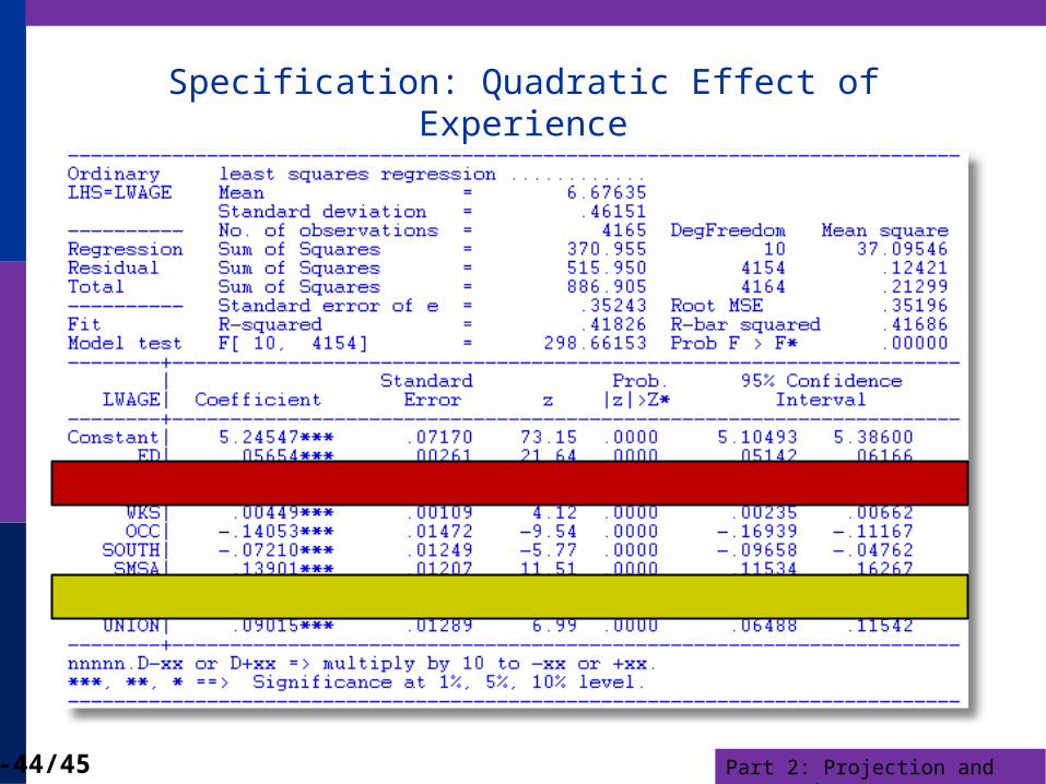
Specification: Quadratic Effect of Experience


Model Implication: Effect of Experience and Male vs. Female

Documents

Part 2: Projection and Regression 2-1/45 Econometrics I Professor William Greene Stern School of Business Department of Economics