Embed Size (px)
Citation preview

Part 5Part 5
© 2006 Thomson Learning/South-Western
Perfect Competition

Chapter 10Chapter 10
© 2006 Thomson Learning/South-Western
Perfect Competition in a Single Market

3
Pricing in the Very Short Run
The market period (very short run) is a short period of time during which quantity supplied is fixed.
In this period, price acts to ration demand as it adjusts to clear the market.
This situation is illustrated in Figure 10-1 where supply is fixed at Q*.

4
Price
S
D
P1
Quantityper week
Q*0
FIGURE 10-1: Pricing in the Very Short Run

5
Pricing in the Very Short Run
When demand is represented by the curve D, P1 is the equilibrium price.
The equilibrium price is the price at which the quantity demanded by buyers of a good is equal to the quantity supplied by sellers of the good.

6
Shifts in Demand: Price as a Rationing Device
If demand were to increase, as illustrated by the new demand curve D’ in Figure 10-1, P1 is no longer the equilibrium price since the quantity demanded exceeds the quantity supplied.
The new equilibrium price is now P2 where price has rationed the good to those who value it the most.

7
Price
P2
S
D
D’P1
Quantityper week
Q*0
FIGURE 10-1: Pricing in the Very Short Run

8
Construction of a Short-Run Supply Curve
The quantity that is supplied is the sum of the quantities supplied by each firm.
The short-run market supply curve is the relationship between market price and quantity supplied of a good in the short run.
In Figure 10-2 it is assumed that there are only two firms, A and B.

9
Price
P
SA
Output
(a) Firm A
0
Price
Output
(b) Firm B
0
Price
Quantityper week
(c) The Market
0
FIGURE 10-2: Short-Run Market Supply Curve
qA1

10
Price
P
SA
Output
(a) Firm A
0
Price
SB
Output
(b) Firm B
0
Price
Quantityper week
(c) The Market
0
FIGURE 10-2: Short-Run Market Supply Curve
qA1 qB
1

11
Price
P
SA
Output
(a) Firm A
0
Price
SB
Output
(b) Firm B
0
Price
S
Quantityper week
(c) The Market
0 Q1
FIGURE 10-2: Short-Run Market Supply Curve
qA1 qB
1

12
Construction of a Short-Run Supply Curve
Both firm A’s and firm B’s short-run supply curves (their marginal cost curves) are shown in Figure 10-2(a) and Figure 10-2(b) respectively.
The market supply curve is the horizontal sum of the two firms at every price. In Figure 10-2(c), Q1 equals the sum of q1
A and q1
B.

13
Short-Run Price Determination
Figure 10-3 (b) shows the market equilibrium where the market demand curve D and the short-run supply curve S intersect at a price of P1 and quantity Q1.
This equilibrium would persist since what firms supply at P1 is exactly what people want to buy at that price.

14
Price SMC
SAC
Output
(a) Typical Firm
0
Price S
D
Quantityper week
(b) The Market
Price
Quantity
(c) Typical Person
0 0
FIGURE 10-3: Interaction of Many Individuals and Firms Determine market price in the Short Run
P1
q1q2 q1 q2 q1‘Q1 Q2
d

15
Price SMC
SAC
Output
(a) Typical Firm
0
Price S
D
Quantityper week
(b) The Market
Price
Quantity
(c) Typical Person
0 0
D’
FIGURE 10-3: Interaction of Many Individuals and Firms Determine market price in the Short Run
P1
P2
q1q2 q1 q2 q1‘Q1 Q2
d
d’

16
Functions of the Equilibrium Price
The price serves as a signal to producers about how much should be produced. To maximize profit, firms will produce the
output level for which marginal costs equal P1.
This yields an aggregate production of Q1.

17
Functions of the Equilibrium Price
Given the price, utility maximizing individuals will decide how much of their limited incomes to spend At price P1 the total quantity demanded is
Q1. No other price brings about the balance of
quantity demanded and quantity supplied. These situations are depicted in Figure
10-3 (a) and (b) for the typical firm and individual, respectively.
18
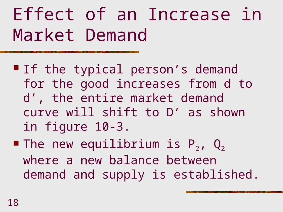
Effect of an Increase in Market Demand
If the typical person’s demand for the good increases from d to d’, the entire market demand curve will shift to D’ as shown in figure 10-3.
The new equilibrium is P2, Q2 where a new balance between demand and supply is established.

19
Effect of an Increase in Market Demand
The increase in demand resulted in a higher equilibrium price, P2 and a greater equilibrium quantity, Q2.
P2 has rationed the typical person’s demand so that only q2 is demanded rather than the q’1 that would have been demanded at P1.
P2 also signals the typical firm to increase production from q1 to q2.

20
Shifts in Demand Curves
Demand will increase, shift outward, because Income increases The price of a substitute rises The price of a complement falls Preferences for the good increase

21
Shifts in Demand Curves
Demand will decrease, shift inward, because Income falls The price of a substitute falls The price of a complement rises Preferences for the good diminish

22
Shifts in Supply Curves
Supply will increase, shift outward, because Input prices fall Technology improves
Supply will decrease, shift inward, because Input prices rise
23
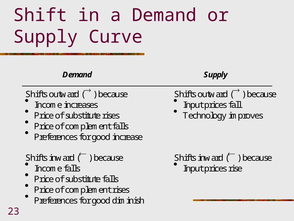
Table 10-1: Reasons for a Shift in a Demand or Supply Curve
Demand Supply Shifts outward ( ) because Shifts outward ( ) because Income increases Input prices fall Price of substitute rises Technology improves Price of complement falls Preferences for good increase Shifts inward ( ) because Shifts inward ( ) because Income falls Input prices rise Price of substitute falls Price of complement rises Preferences for good diminish

24
Short-Run Supply Elasticity
The short-run elasticity of supply is the percentage change in quantity supplied in the short run in response to a 1 percent change in price.
[10.1] price in change Percentage
run short in supplied
quantity in change Percentage
elasticitysupply run-Short .

25
Shifts in Supply Curves and the Importance of the Shape of the Demand Curve
The effect of a shift in supply upon equilibrium levels of P and Q depends upon the shape of the demand curve. If demand is elastic, as in Figure 10-4 (a),
a decrease in supply has a small effect on price but a relatively large effect on quantity.
If demand is inelastic, as in Figure 10-4 (b), the decrease in supply has a greater effect on price than on quantity.

26
Price
P
(a) Elastic Demand
Q
S
D
0 Quantityper week
(b) Inelastic Demand
Price
S
D
P
0 QQuantityper week
FIGURE 10-4: Effect of a Shift in the Short-Run Supply Curve on the Shape of the Demand Curve

27
Price
P
(a) Elastic Demand
Q
S
D
0 Quantityper week
(b) Inelastic Demand
PriceS’
SS’
D
P
P’
P’
0Q’ QQ’Quantityper week
FIGURE 10-4: Effect of a Shift in the Short-Run Supply Curve on the Shape of the Demand Curve

28
Shifts in Demand Curves and the Importance of the Shape of the Supply Curve
The effect of a shift in demand upon equilibrium levels of P and Q depends upon the shape of the supply curve. If supply is inelastic, as in Figure 10-5 (a), the
effect on price is much greater than on quantity.
If the supply curve is elastic, as in Figure 10-5 (b), the effect on price is relatively smaller than the effect on quantity.

29
Quantityper week
(a) Inelastic Supply
S
(b) Elastic Supply
S
Quantityper week
Q Q
P P
P’
PricePrice
0 0
D D
Figure 10-5: Effect of A shift in the Demand Curve Depends on the Shape of the Short-Run Supply Curve

30
Quantityper week
(a) Inelastic Supply
S
(b) Elastic Supply
S
Quantityper week
Q Q’ Q Q’
P PP’
P’
PricePrice
0 0
D D
D’D’
Figure 10-5: Effect of A shift in the Demand Curve Depends on the Shape of the Short-Run Supply Curve

31
Price
10
6
2
CDs per week
4 10
S
D0
FIGURE 10-6: Demand and Supply Curves for CDs

32
Price
$12
10
765
2
CDsper week3456 1012
S
D0
D’
FIGURE 10-6: Demand and Supply Curves for CDs

33
TABLE 10-2: Supply and Demand Equilibrium in the Market for CDs
Supply Demand
Price
Q = P - 2 Quantity Supplied (CDs per Week)
Case 1 Q = 10 – P Quantity Demanded (CDs per Week)
Case 2 q = 12 – P Quantity Demanded (CDs per Week)
$10 8 0 2 9 7 1 3 8 6 2 4 7 5 3 5 6 4 4 6 5 3 5 7 4 2 6 8 3 1 7 9 2 0 8 10 1 0 9 11 0 0 10 12
New equilibrium Initial equilibrium

34
Profit Maximization
It is assumed that the goal of each firm is to maximize profits. Since each firm is a price taker, this implies
that each firm produce where price equals long-run marginal cost.
This equilibrium condition, P = MC determines the firm’s output choice and its choice of inputs that minimize their long-run costs.

35
Entry and Exit
Entry will cause the short-run market supply curve to shift outward causing the market price to fall. This will continue until positive economic
profits are no longer available. Exit causes the short-run market supply
curve to shift inward causing the market price to increase, eliminating the economic losses.

36
Long-Run Equilibrium
P = MC results from the assumption that firm’s are profit maximizers.
P = AC results because market forces cause long run economic profits to equal zero.
In the long run, firm owners will only earn normal returns on their investments.

37
Long-Run Supply: The Constant Cost Case
The constant cost case is a market in which entry or exit has no effect on the cost curves of firms.
Figure 10-7 demonstrates long-run equilibrium for the constant cost case.
Figure 10-7 (b) shows that market where the market demand and supply curves are D and S, respectively, and equilibrium price is P1.

38
Price SMCS
D
MCAC
Output
(a) Typical Firm
0
Price
Quantityper week
(b) Total Market
0
FIGURE 10-7: Long-Run Equilibrium for a Perfectly Competitive Market: Constant Cost Case
q1 Q1
P1

39
Price SMCS
D
D
MCAC
Output
(a) Typical Firm
0
Price
Quantityper week
(b) Total Market
Q20
FIGURE 10-7: Long-Run Equilibrium for a Perfectly Competitive Market: Constant Cost Case
q1q2 Q1
P1
P2

40
Price SMCS
S’
D
D
LS
MCAC
Output
(a) Typical Firm
0
Price
Quantityper week
(b) Total Market
Q20
FIGURE 10-7: Long-Run Equilibrium for a Perfectly Competitive Market: Constant Cost Case
q1 q2 Q3Q1
P1
P2

41
Long-Run Supply: The Constant Cost Case
The typical firm will produce output level q1 which results in Q1 in the market.
The typical firm is maximizing profits since price is equal to long-run marginal cost.
The typical firm is earning zero economic profits since price equals long-run average total costs.
There is no incentive for exit or entry.

42
A Shift in Demand
If demand increases to D’, the short-run price will increase to P2.
A typical firm will maximize profits by producing q2 which will result in short-run economic profits (P2 > AC).
Positive economic profits cause new firms to enter the market until economic profits again equal zero.

43
A Shift in Demand
Since costs do not increase with entry, the typical firm’s costs curves do not change.
The supply curve shifts to S’ where the equilibrium price returns to P1 and the typical firm produces q1 again.
The new long-run equilibrium output will be Q3 with more firms in the market.
44
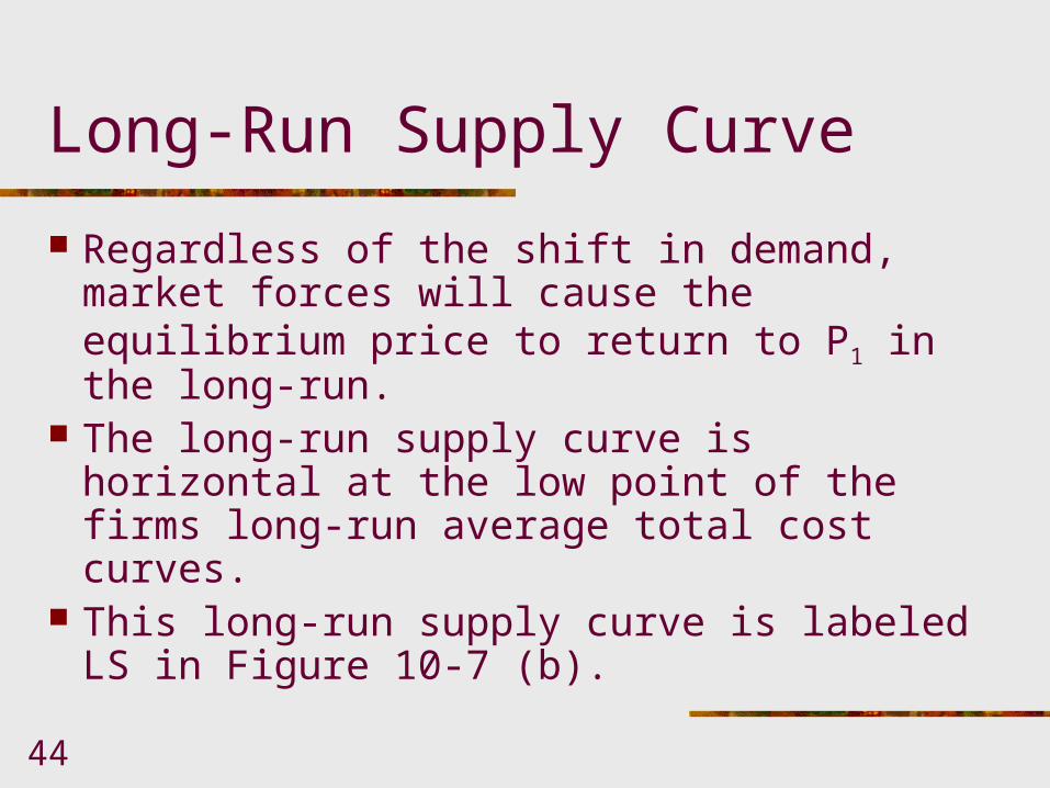
Long-Run Supply Curve
Regardless of the shift in demand, market forces will cause the equilibrium price to return to P1 in the long-run.
The long-run supply curve is horizontal at the low point of the firms long-run average total cost curves.
This long-run supply curve is labeled LS in Figure 10-7 (b).

45
Price
P1
SMC
MCAC
D
S
(a) Typical Firm before Entry
q1 q20 Output
(b) Typical Firm after Entry
Quantityper week
(c) The Market
Q1
2
FIGURE 10-8: Increasing Costs Result in a Positively Sloped Long-Run Supply Curve
SMC
MC
AC
Output q3
P1
P3
P2
P3
0 0
Price Price

46
Price
P1
SMC
MCAC
D
S
(a) Typical Firm before Entry
q1 q20 Output
(b) Typical Firm after Entry
Quantityper week
(c) The Market
Q1
2
FIGURE 10-8: Increasing Costs Result in a Positively Sloped Long-Run Supply Curve
SMCMC
AC
Output q3
P1
P2P2
Q3Q2
D’
0 0
Price Price

47
Price
P1
SMC
MCAC
D
S
LS
(a) Typical Firm before Entry
q1 q20 Output
(b) Typical Firm after Entry
Quantityper week
(c) The Market
Q1
2
FIGURE 10-8: Increasing Costs Result in a Positively Sloped Long-Run Supply Curve
SMCMC
AC
Output q3
P1
P3
P2
P3
P2
Q3Q2
D’ S’
0 0
Price Price
48
The Increasing Cost Case
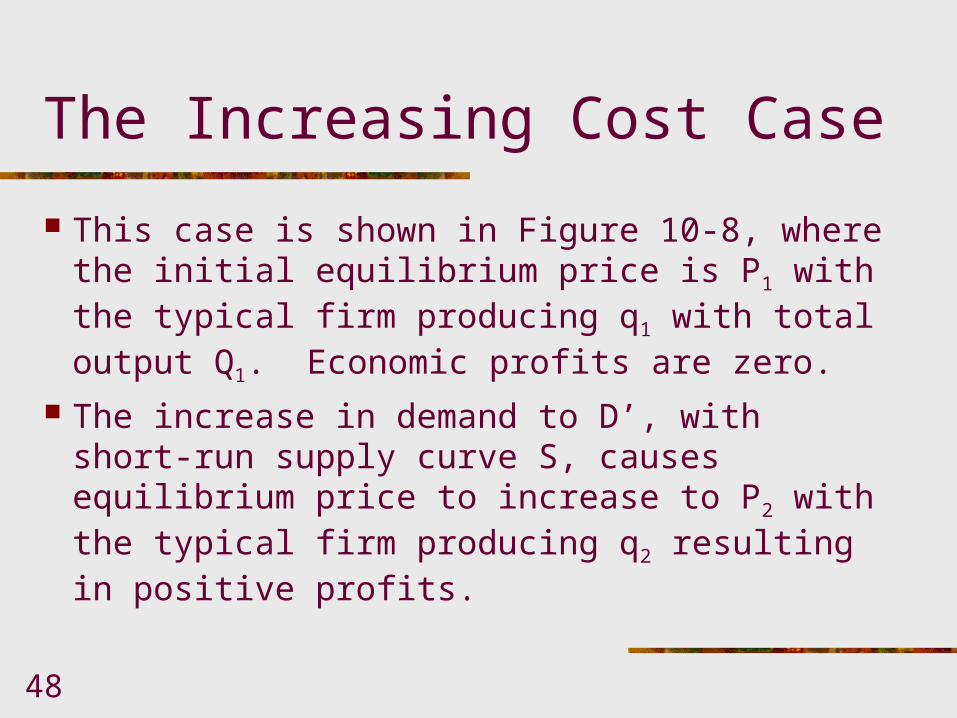
This case is shown in Figure 10-8, where the initial equilibrium price is P1 with the typical firm producing q1 with total output Q1. Economic profits are zero.
The increase in demand to D’, with short-run supply curve S, causes equilibrium price to increase to P2 with the typical firm producing q2 resulting in positive profits.

49
The Increasing Cost Case
The positive profits entice firms to enter which drives up costs.
The typical firm’s new cost curves are shown in Figure 10-8 (b).
The new long-run equilibrium price is P3 with market output Q3.
The long-run supply curve, LS, is positively sloped because of the increasing costs.

50
Long-Run Supply Elasticity
The long-run elasticity of supply is the percentage change in quantity supplied in the long run in response to a 1 percent change in price.
[10.5] price in change Percentage
run long the in supplied
quantity in change Percentage
supply of elasticity run-Long
51
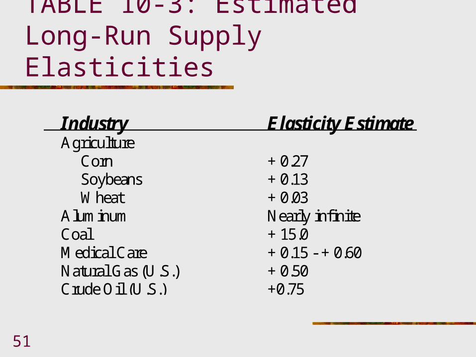
TABLE 10-3: Estimated Long-Run Supply Elasticities
Industry Elasticity EstimateAgriculture Corn + 0.27 Soybeans + 0.13 Wheat + 0.03Aluminum Nearly infiniteCoal + 15.0Medical Care + 0.15 - + 0.60Natural Gas (U.S.) + 0.50Crude Oil (U.S.) +0.75

52
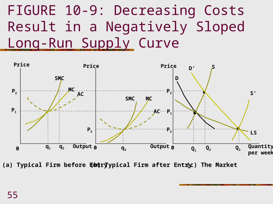
The Decreasing Cost Case
The initial equilibrium is shown as P1, Q1 in Figure 10-9 (c).
The increase in demand from D to D’ results in the short-run equilibrium, P2, Q2 where the typical firm is earning positive economic profits.
Entry drives down costs for the typical firm, as shown in Figure 10-9 (b).

53
Price
P1
SMC
MCAC
D
S
(a) Typical Firm before Entry
q10 Output
(b) Typical Firm after Entry
Quantityper week
(c) The Market
Q1
2
FIGURE 10-9: Decreasing Costs Result in a Negatively Sloped Long-Run Supply Curve
SMC MC
AC
Output
P1
P2
Price Price
0 0

54
Price
P1
SMC
MCAC
D
S
(a) Typical Firm before Entry
q1 q20 Output
(b) Typical Firm after Entry
Quantityper week
(c) The Market
Q1
2
FIGURE 10-9: Decreasing Costs Result in a Negatively Sloped Long-Run Supply Curve
SMC MC
AC
Output
P1
P2P2
Q2
D’Price Price
0 0
55
Price
P1
SMC
MCAC
D
S
LS
(a) Typical Firm before Entry
q1 q20 Output
(b) Typical Firm after Entry
Quantityper week
(c) The Market
Q1
2
FIGURE 10-9: Decreasing Costs Result in a Negatively Sloped Long-Run Supply Curve
SMC MC
AC
Output q3
P1
P3
P2
P3
P2
Q3Q2
D’
S’
Price Price
0 0

56
The Decreasing Cost Case
Entry continues until short-run economic profits are eliminated.
The new long-run equilibrium is P3, Q3 as shown in Figure 10-9 (c).
The long-run supply curve is downward sloping due to the decreasing costs as labeled LS in Figure 10-9 (c).