Embed Size (px)
Citation preview

Part OneExploratory Data Analysis
ProbabilityDistributions
Charles A. Rohde
Fall 2001
Contents
1 Numeracy and Exploratory Data Analysis 1
1.1 Numeracy . . . . . . . . . . . . . . . . . . . . . . . . . . . . . . . . . . . . . 1
1.1.1 Numeracy . . . . . . . . . . . . . . . . . . . . . . . . . . . . . . . . . 1
1.2 Discrete Data . . . . . . . . . . . . . . . . . . . . . . . . . . . . . . . . . . . 3
1.3 Stem and leaf displays . . . . . . . . . . . . . . . . . . . . . . . . . . . . . . 6
1.4 Letter Values . . . . . . . . . . . . . . . . . . . . . . . . . . . . . . . . . . . 9
1.5 Five Point Summaries and Box Plots . . . . . . . . . . . . . . . . . . . . . . 12
1.6 EDA Example . . . . . . . . . . . . . . . . . . . . . . . . . . . . . . . . . . . 14
1.7 Other Summaries . . . . . . . . . . . . . . . . . . . . . . . . . . . . . . . . . 21
1.7.1 Classical Summaries . . . . . . . . . . . . . . . . . . . . . . . . . . . 22
1.8 Transformations for Symmetry . . . . . . . . . . . . . . . . . . . . . . . . . . 23
1.9 Bar Plots and Histograms . . . . . . . . . . . . . . . . . . . . . . . . . . . . 27
1.9.1 Bar Plots . . . . . . . . . . . . . . . . . . . . . . . . . . . . . . . . . 27
1.9.2 Histograms . . . . . . . . . . . . . . . . . . . . . . . . . . . . . . . . 27
1.9.3 Frequency Polygons . . . . . . . . . . . . . . . . . . . . . . . . . . . . 30
1.10 Sample Distribution Functions . . . . . . . . . . . . . . . . . . . . . . . . . . 32
1.11 Smoothing . . . . . . . . . . . . . . . . . . . . . . . . . . . . . . . . . . . . 34
i

ii CONTENTS
1.11.1 Smoothing Example . . . . . . . . . . . . . . . . . . . . . . . . . . . 36
1.12 Shapes of Batches . . . . . . . . . . . . . . . . . . . . . . . . . . . . . . . . . 42
1.13 References . . . . . . . . . . . . . . . . . . . . . . . . . . . . . . . . . . . . . 43
2 Probability 47
2.1 Mathematical Preliminaries . . . . . . . . . . . . . . . . . . . . . . . . . . . 47
2.1.1 Sets . . . . . . . . . . . . . . . . . . . . . . . . . . . . . . . . . . . . 47
2.1.2 Counting . . . . . . . . . . . . . . . . . . . . . . . . . . . . . . . . . . 52
2.2 Relating Probability to Responses and Populations . . . . . . . . . . . . . . 54
2.3 Probability and Odds - Basic Definitions . . . . . . . . . . . . . . . . . . . . 56
2.3.1 Probability . . . . . . . . . . . . . . . . . . . . . . . . . . . . . . . . 56
2.3.2 Properties of Probability . . . . . . . . . . . . . . . . . . . . . . . . . 57
2.3.3 Methods for Obtaining Probability Models . . . . . . . . . . . . . . . 58
2.3.4 Odds . . . . . . . . . . . . . . . . . . . . . . . . . . . . . . . . . . . . 61
2.4 Interpretations of Probability . . . . . . . . . . . . . . . . . . . . . . . . . . 64
2.4.1 Equally Likely Interpretation . . . . . . . . . . . . . . . . . . . . . . 64
2.4.2 Relative Frequency Interpretation . . . . . . . . . . . . . . . . . . . . 65
2.4.3 Subjective Probability Interpretation . . . . . . . . . . . . . . . . . . 65
2.4.4 Does it Matter? . . . . . . . . . . . . . . . . . . . . . . . . . . . . . . 66
2.5 Conditional Probability . . . . . . . . . . . . . . . . . . . . . . . . . . . . . . 67
2.5.1 Multiplication Rule . . . . . . . . . . . . . . . . . . . . . . . . . . . . 69
2.5.2 Law of Total Probability . . . . . . . . . . . . . . . . . . . . . . . . . 71
2.6 Bayes Theorem . . . . . . . . . . . . . . . . . . . . . . . . . . . . . . . . . . 75
2.7 Independence . . . . . . . . . . . . . . . . . . . . . . . . . . . . . . . . . . . 80
2.8 Bernoulli trial models; the binomial distribution . . . . . . . . . . . . . . . . 81

CONTENTS iii
2.9 Parameters and Random Sampling . . . . . . . . . . . . . . . . . . . . . . . 83
2.10 Probability Examples . . . . . . . . . . . . . . . . . . . . . . . . . . . . . . . 94
2.10.1 Randomized Response . . . . . . . . . . . . . . . . . . . . . . . . . . 94
2.10.2 Screening . . . . . . . . . . . . . . . . . . . . . . . . . . . . . . . . . 96
3 Probability Distributions 99
3.1 Random Variables and Distributions . . . . . . . . . . . . . . . . . . . . . . 99
3.1.1 Introduction . . . . . . . . . . . . . . . . . . . . . . . . . . . . . . . . 99
3.1.2 Discrete Random Variables . . . . . . . . . . . . . . . . . . . . . . . . 101
3.1.3 Continuous or Numeric Random Variables . . . . . . . . . . . . . . . 107
3.1.4 Distribution Functions . . . . . . . . . . . . . . . . . . . . . . . . . . 116
3.1.5 Functions of Random Variables . . . . . . . . . . . . . . . . . . . . . 117
3.1.6 Other Distributions . . . . . . . . . . . . . . . . . . . . . . . . . . . . 118
3.2 Parameters of Distributions . . . . . . . . . . . . . . . . . . . . . . . . . . . 119
3.2.1 Expected Values . . . . . . . . . . . . . . . . . . . . . . . . . . . . . 119
3.2.2 Variances . . . . . . . . . . . . . . . . . . . . . . . . . . . . . . . . . 121
3.2.3 Quantiles . . . . . . . . . . . . . . . . . . . . . . . . . . . . . . . . . 122
3.2.4 Other Expected Values . . . . . . . . . . . . . . . . . . . . . . . . . . 123
3.2.5 Inequalities involving Expectations . . . . . . . . . . . . . . . . . . . 125
4 Joint Probability Distributions 127
4.1 General Case . . . . . . . . . . . . . . . . . . . . . . . . . . . . . . . . . . . 127
4.1.1 Marginal Distributions . . . . . . . . . . . . . . . . . . . . . . . . . . 128
4.1.2 Conditional Distributions . . . . . . . . . . . . . . . . . . . . . . . . 128
4.1.3 Properties of Marginal and Conditional Distributions . . . . . . . . . 129
4.1.4 Independence and Random Sampling . . . . . . . . . . . . . . . . . . 129

iv CONTENTS
4.2 The Multinomial Distribution . . . . . . . . . . . . . . . . . . . . . . . . . . 130
4.3 The Multivariate Normal Distribution . . . . . . . . . . . . . . . . . . . . . . 134
4.4 Parameters of Joint Distributions . . . . . . . . . . . . . . . . . . . . . . . . 136
4.4.1 Means, Variances, Covariances and Correlation . . . . . . . . . . . . 136
4.4.2 Joint Moment Generating Functions . . . . . . . . . . . . . . . . . . 138
4.5 Functions of Jointly Distributed Random Variables . . . . . . . . . . . . . . 139
4.5.1 Linear Combinations of Random Variables . . . . . . . . . . . . . . . 141
4.6 Approximate Means and Variances . . . . . . . . . . . . . . . . . . . . . . . 143
4.7 Sampling Distributions of Statistics . . . . . . . . . . . . . . . . . . . . . . . 145
4.8 Methods of Obtaining Sampling Distibutions or Approximations . . . . . . . 151
4.8.1 Exact Sampling Distributions . . . . . . . . . . . . . . . . . . . . . . 151
4.8.2 Asymptotic Distributions . . . . . . . . . . . . . . . . . . . . . . . . . 152
4.8.3 Central Limit Theorem . . . . . . . . . . . . . . . . . . . . . . . . . . 152
4.8.4 Central Limit Theorem Example . . . . . . . . . . . . . . . . . . . . 153
4.8.5 Law of Large Numbers . . . . . . . . . . . . . . . . . . . . . . . . . . 158
4.8.6 The Delta Method - Univariate . . . . . . . . . . . . . . . . . . . . . 160
4.8.7 The Delta Method - Multivariate . . . . . . . . . . . . . . . . . . . . 162
4.8.8 Computer Intensive Methods . . . . . . . . . . . . . . . . . . . . . . 166
4.8.9 Bootstrap Example . . . . . . . . . . . . . . . . . . . . . . . . . . . 170

Chapter 1
Numeracy and Exploratory DataAnalysis
1.1 Numeracy
1.1.1 Numeracy
Since most of statistics involves the use of numerical data to draw conclusions we first discussthe presentation of numerical data.
Numeracy may be broadly defined as the ability to effectively think about and presentnumbers.
• One of the most common forms of presentation of numerical information is in tables.
• There are some simple guidelines which allow us to improve tabular presentation ofnumbers.
• In certain situations, the guidelines presented here will need to be modified if theaudience e.g. readers of a professional journal expect the results to be presented in aspecified format.
1

2 CHAPTER 1. NUMERACY AND EXPLORATORY DATA ANALYSIS
Guidelines
• Round to two significant figures.
In order to understand a table of numbers it is almost always easier to do so ifthe numbers do not contain too many significant figures.
• Add averages or totals.
Adding row and/or column averages, proportions or totals when appropriate to atable often provide a useful focus for establishing trends or patterns.
• Numbers are easier to compare in columns.
• Order by size.
A more effective presentation is often achieved by rearranging so that the largest(and presumably most important numbers) appear first.
• Spacing and layout.
It is useful to present tables in single space format and not have a lot of “emptyspace” to detract the reader from concentrating on the numbers in the table.

1.2. DISCRETE DATA 3
1.2 Discrete Data
For discrete data present tables of the numbers of responses at the various values, possiblygrouped by factors. Also one can produce bar graphs and histograms for graphical pre-sentation. Thus in the first example in the introduction we might present the results asfollows:
Placebo VaccineProportion Cases .008 .004Studied 200,745 201,229
A sensible description might be 4 cases per thousand for the vaccinated group and 8 casesper thousand for the placebo group.

4 CHAPTER 1. NUMERACY AND EXPLORATORY DATA ANALYSIS
For the alcohol use data in the Overview Section eg.
Group Use Alcohol Surveyed ProportionClergy 32 300 .11Educators 51 250 .20Executives 67 300 .22Merchants 83 350 .24
we might present the data as
Figure 1.1:

1.2. DISCRETE DATA 5
For the self classification data in the Overview Section e.g.
Class Lower Working Middle UpperNumber 72 714 655 41
we might present the data as
Figure 1.2:

6 CHAPTER 1. NUMERACY AND EXPLORATORY DATA ANALYSIS
1.3 Stem and leaf displays
Suppose we have a batch or collection of numbers. Stem and leaf displays provide a simple,yet informative way to
• Develop summaries or descriptions of the batch either to learn about it in isolation orto compare it with other batches. The fundamental summaries are
location of the batch (a center concept)
scale or spread of the batch (a variability concept).
• Explore (note) characteristics of the batch including
symmetry and general shape
exceptional values
gaps
concentrations

1.3. STEM AND LEAF DISPLAYS 7
Consider the following batch of 62 numbers which give the ages in years of graduatestudents, post-docs, staff and faculty of a large academic department of statistics:
33 20 41 52 35 25 43 61 37 29 44 64 40 32 50 76
33 22 42 55 36 26 43 61 37 30 46 65 40 32 50 79
34 23 43 59 37 27 43 61 39 31 46 67 41 32 51 81
37 28 44 64 37 29 44 64 40 31 49 74 51 52
Not much can be learned by looking at the numbers in this form.
A simple display which begins to describe this collection of numbers is as follows:
9 |
( 1) 1 8 | 1
( 4) 3 7 | 4 6 9
(12) 8 6 | 1 4 5 7 4 1 1 4
(20) 8 5 | 9 1 5 2 1 2 0 0
(42) 16 4 | 2 1 4 3 3 3 0 3 6 0 1 6 4 0 9 4
(26) 17 3 | 0 7 6 3 7 2 7 2 2 2 1 5 9 4 7 1 7
( 9) 9 2 | 9 7 3 2 9 0 5 6 8
1 |
|
Interpretation: 1 at 8 means 81, 4 at 7 means 74, 6 at 7 means 76, 9 at 7 means 79,etc.

8 CHAPTER 1. NUMERACY AND EXPLORATORY DATA ANALYSIS
A more refined version of this display is:
9 |
( 1) 1 8 | 1
( 4) 3 7 | 4 6 9
(12) 8 6 | 1 1 1 4 4 4 5 7
(20) 8 5 | 0 0 1 1 2 2 5 9
(42) 16 4 | 0 0 0 1 1 2 3 3 3 3 4 4 4 6 6 9
(26) 17 3 | 0 1 1 2 2 2 3 3 4 5 6 7 7 7 7 7 9
( 9) 9 2 | 0 2 3 5 6 7 8 9 9
1 |
Interpretation: 1 at 8 means 81, 4 at 7 means 74, 6 at 7 means 76, 9 at 7 means 79, etc.
To construct a stem and leaf display we perform the following steps:
• To the left of the solid line we put the stem of the number
• To the right of the solid line we put the leaf of the number.
The remaining entries in the display are discussed in the next section. Note that a stem andleaf display provides a quick and easy way to display a batch of numbers. Every statisticalpackage now has a program to draw stem and leaf displays.
Some additional comments on stem and leaf displays:
• Number of stems. Understanding Robust and Exploratory Data Analysis suggests√
nfor n less than 100 and 10 log10(n) for n larger than 100.
(Usually more than 50 are done using a computer and each statistical package has itsown default method).
• Stems can be double (or more) digits and there can be stems such as 5? and 5· whichdivide the numbers with stem 5 into two groups (0,1,2,3,4) and (5,6,7,8,9). Largedisplays could use 5 or 10 divisions per stem. The important idea is to display thenumbers effectively.
• For small batches, when working by hand, the use of stem and leaf displays is a simpleway to obtain the ordered values of the batch.

1.4. LETTER VALUES 9
1.4 Letter Values
The stem and leaf display can be used to determine a collection of derived numbers, calledstatistics, which can be used to summarize some additional features of the batch. To do thiswe need determine the total size of the batch and where the individual numbers are locatedin the display.
• To the left of the stem we count the number of leaves on each stem.
• The numbers in parentheses are the cumulative numbers counting up and countingdown.
• Using the stem and leaf display we can easily “count in” from either end of the batch.
The associated count is called the depth of the number.
Thus at depth 4 we have the number 74 if we count down (largest to smallest)and the number 25 if we count up (smallest to largest).
• It is easier to understand the concept of depth if the numbers are written in a columnfrom largest to smallest.
• A measure of location is provided by the median, defined as that number in the displaywith depth equal to
1
2(1 + batch size)
If the size of the batch is even (n = 2m) the depth of the median will not be aninteger.
In such a case the median is defined to be halfway between the numbers withdepth m and depth m + 1.
In the example
median depth =1
2(1 + 62) =
63
2= 31.5
thus the median is given by:
(# with depth 31) + (# with depth 32)
2=
41 + 42
2= 41.5

10 CHAPTER 1. NUMERACY AND EXPLORATORY DATA ANALYSIS
The median has the property that 1/2 of the numbers in the batch are above itand 1/2 of the numbers in the batch are below it, i.e., it is halfway from eitherend of the batch.
• The median is just one example of a letter value. Other letter values enable us todescribe variability, shape and other characteristics of the batch.
The simplest sequence of letter values divides the lower half in two and the upperhalf in two, each of these halves in two, and so on.
To obtain these letter values we first find their depths by the formula
next letter value depth =1
2(1 + [previous letter value depth])
where [ ] means we discard any fraction in the calculation. (Called the “floorfunction”).
Thus the upper and lower quartiles have depths equal to
1
2(1 + [depth of median])
The quartiles are sometimes called fourths.
The eighths have depths equal to
1
2(1 + [depth of hinge])
We proceed down to the extremes which have depth 1.
The median, quartiles and extremes often describe a batch of numbers quite well.
The remaining letter values are used to describe more subtle features of the data(illustrated later).
In the example we thus have
F depth =1
2(1 + 31) =
32
2= 16
E depth =1
2(1 + 16) =
17
2= 8.5
Extreme depth =1
2(1 + 1) =
2
2= 1
The corresponding letter values are

1.4. LETTER VALUES 11
M 41.5 depth 31.5F 33 52 depth 16Ex 20 81 depth 1
We can display the letter values as follows:
Value Depth Lower Upper SpreadM 31.5 41.5 41.5 0F 16 33 52 19E 8.5 29 64 35Ex 1 20 81 61
where the spread of a letter value is defined as:
upper letter value− lower letter value

12 CHAPTER 1. NUMERACY AND EXPLORATORY DATA ANALYSIS
1.5 Five Point Summaries and Box Plots
• A useful summary of a batch of numbers is the five point summary in which we listthe upper and lower extremes, the upper and lower hinges and the median. Thus forthe example we have the five point summary given by
20, 33, 41.5, 52, 81
• A five point summary can be displayed graphically as a box plot in which we pictureonly the median, the lower fourth, the upper fourth and the extremes as on the followingpage:

1.5. FIVE POINT SUMMARIES AND BOX PLOTS 13
For this batch of numbers there is evidence of asymmetry or skewness as can beobserved from the stem-leaf display or the box plot.
Figure 1.3:
To measure spread we can use the interquartile range which is simply the diferencebetween the upper quartile and the lower quartile.

14 CHAPTER 1. NUMERACY AND EXPLORATORY DATA ANALYSIS
1.6 EDA Example
The following are the heights in centimeters of 351 elderly female patients. The data set iselderly.raw (from Hand et. al. pages 120-121)
156 163 169 161 154 156 163 164 156 166 177 158150 164 159 157 166 163 153 161 170 159 170 157156 156 153 178 161 164 158 158 162 160 150 162155 161 158 163 158 162 163 152 173 159 154 155164 163 164 157 152 154 173 154 162 163 163 165160 162 155 160 151 163 160 165 166 178 153 160156 151 165 169 157 152 164 166 160 165 163 158153 162 163 162 164 155 155 161 162 156 169 159159 159 158 160 165 152 157 149 169 154 146 156157 163 166 165 155 151 157 156 160 170 158 165167 162 153 156 163 157 147 163 161 161 153 155166 159 157 152 159 166 160 157 153 159 156 152151 171 162 158 152 157 162 168 155 155 155 161157 158 153 155 161 160 160 170 163 153 159 169155 161 156 153 156 158 164 160 157 158 157 156160 161 167 162 158 163 147 153 155 159 156 161158 164 163 155 155 158 165 176 158 155 150 154164 145 153 169 160 159 159 163 148 171 158 158157 158 168 161 165 167 158 158 161 160 163 163169 163 164 150 154 165 158 161 156 171 163 170154 158 162 164 158 165 158 156 162 160 164 165157 167 142 166 163 163 151 163 153 157 159 152169 154 155 167 164 170 174 155 157 170 159 170155 168 152 165 158 162 173 154 167 158 159 152158 167 164 170 164 166 170 160 148 168 151 153150 165 165 147 162 165 158 145 150 164 161 157163 166 162 163 160 162 153 168 163 160 165 156158 155 168 160 153 163 161 145 161 166 154 147161 155 158 161 163 157 156 152 156 165 159 170160 152 153

1.6. EDA EXAMPLE 15
STATA log for EDA of Heights of Elderly Women
. infile height using c:\courses\b651201\datasets\elderly.raw
(351 observations read)
. stem height
Stem-and-leaf plot for height
14t | 2
14f | 555
14s | 67777
14. | 889
15* | 000000111111
15t | 22222222222233333333333333333
15f | 44444444444555555555555555555555
15s | 6666666666666666666677777777777777777777
15. | 888888888888888888888888888888899999999999999999
16* | 00000000000000000000011111111111111111111
16t | 222222222222222222333333333333333333333333333333
16f | 44444444444444444555555555555555555
16s | 666666666667777777
16. | 88888899999999
17* | 00000000000111
17t | 333
17f | 4
17s | 67
17. | 88

16 CHAPTER 1. NUMERACY AND EXPLORATORY DATA ANALYSIS
. summarize height, detail
height
-------------------------------------------------------------
Percentiles Smallest
1% 145 142
5% 150 145
10% 152 145 Obs 351
25% 156 145 Sum of Wgt. 351
50% 160 Mean 159.7749
Largest Std. Dev. 6.02974
75% 164 176
90% 168 177 Variance 36.35777
95% 170 178 Skewness .1289375
99% 176 178 Kurtosis 3.160595
. display 3.49*6.02974*(351^(-1/3))
2.9832408
. display 3.49*sqrt(r(Var))*(351^(-1/3))
2.983241
. display (178-142)/2.98
12.080537
. display min(sqrt(351),10*log(10))
18.734994

1.6. EDA EXAMPLE 17
. graph height, normal xlabel ylabel ti(Heights of Elderly Women 5 Bins)
. graph height, normal xlabel ylabel ti(Heights of Elderly Women 5 Bins) saving
> (g1,replace)
. graph height, bin(12) normal xlabel ylabel ti(Heights of Elderly Women 5 Bins
> ) saving(g2,replace)
. graph height, bin(12) normal xlabel ylabel ti(Heights of Elderly Women 12 Bin
> s) saving(g2,replace)
. graph height, bin(18) normal xlabel ylabel ti(Heights of Elderly Women 18 Bin
> s) saving(g3,replace)
. graph height, bin(25) normal xlabel ylabel ti(Heights of Elderly Women 25 Bin
> s) saving(g4,replace)
. graph using g1 g2 g3 g4

18 CHAPTER 1. NUMERACY AND EXPLORATORY DATA ANALYSIS
Histograms of Data on Elderly Women
Figure 1.4: Histograms

1.6. EDA EXAMPLE 19
. lv height
# 351 height
---------------------------------
M 176 | 160 | spread pseudosigma
F 88.5 | 156 160 164 | 8 5.95675
E 44.5 | 153 159.5 166 | 13 5.667454
D 22.5 | 151 160.25 169.5 | 18.5 6.048453
C 11.5 | 148.5 159.5 170.5 | 22 5.929273
B 6 | 147 160 173 | 26 6.071367
A 3.5 | 145 160.75 176.5 | 31.5 6.659417
Z 2 | 145 161.5 178 | 33 6.360923
Y 1.5 | 143.5 160.75 178 | 34.5 6.355203
1 | 142 160 178 | 36 6.246375
| | # below # above
inner fence | 144 176 | 1 4
outer fence | 132 188 | 0 0
. format height %9.2f
. lv height
# 351 height
---------------------------------
M 176 | 160.00 | spread pseudosigma
F 88.5 | 156.00 160.00 164.00 | 8.00 5.96
E 44.5 | 153.00 159.50 166.00 | 13.00 5.67
D 22.5 | 151.00 160.25 169.50 | 18.50 6.05
C 11.5 | 148.50 159.50 170.50 | 22.00 5.93
B 6 | 147.00 160.00 173.00 | 26.00 6.07
A 3.5 | 145.00 160.75 176.50 | 31.50 6.66
Z 2 | 145.00 161.50 178.00 | 33.00 6.36
Y 1.5 | 143.50 160.75 178.00 | 34.50 6.36
1 | 142.00 160.00 178.00 | 36.00 6.25
| | # below # above
inner fence | 144.00 176.00 | 1 4
outer fence | 132.00 188.00 | 0 0

20 CHAPTER 1. NUMERACY AND EXPLORATORY DATA ANALYSIS
. graph height, box
. graph height, box ylabel
. graph height, box ylabel l1(Height in Centimeters) ti(Box Plot of Heights of
> Elderly Women)
. cumul height, gen(cum)
. graph cum height,s(i) c(l) ylabel xlabel ti(Empirical Distribution Function O
> f Heights of Elderly Women) rlabel yline(.25,.5,.75)
. kdensity height
. kdensity height,normal ti(Kdensity Estimate of Heights)
. log close

1.7. OTHER SUMMARIES 21
1.7 Other Summaries
Other measures of location are
• mid = 12(UQ + LQ)
• tri-mean = 12(mid + median) = LQ + 2M + UQ
4where UQ is the upper quartile, M
is the median and LQ is the lower quartile.
It is often useful to identify exceptional values that need special attention. We do thisusing fences.
• The upper and lower fences are defined by
upper fence = UF = upper hinge +32(H-spread)
lower fence = LF = lower hinge −32(H-spread)
• Values above the upper fence or below the lower fence can be considered as exceptionalvalues and need to be examined closely for validity.

22 CHAPTER 1. NUMERACY AND EXPLORATORY DATA ANALYSIS
1.7.1 Classical Summaries
The summary quantities developed in the previous sections are examples of statistics, for-mally defined as functions of a sample data set. There are other summary measures of asample data set.
• For location, the traditional summary measure is the sample mean defined by
x =1
n
n∑
i=1
xi
where n is the number of observations in the data set and (x1, x2, . . . , xn) is the sampledata set.
• For spread or variablity the sample variance, s2, and the sample standard deviation,s, are defined by
s2 =1
n− 1
n∑
i=1
(xi − x)2 and s =√
s2
• Note that
x =(1− 1
n
)x(i−1) +
1
nxi
where xi−1 is the sample mean of the data set with the ith observation removed.
It follows that a single observation can greatly influence the magnitude of thesample mean which explains why other summaries such as the median or tri-meanfor location are often used.
Similarly the sample variance and sample standard deviation are greatly influ-enced by single observations.
• For distributions which are “bell-shaped” the interquartile range is approximately equalto 1.34 s to where s is the sample standard deviation.
1.8. TRANSFORMATIONS FOR SYMMETRY 23
1.8 Transformations for Symmetry
Data can be easier to understand if it is nearly symmetric and hence we sometimes transforma batch to make it approximately symmetric. The reasons for transformations are:
• For symmetric batches we have an unambiguous measure of center (the mean or themedian).
• Transformed data may have a scientific meaning.
• Many statistical methods are more reliable for symmetric data.
As examples of transformed data with scientific meaning we have
• For income and population changes the natural logarithm is often useful since bothmoney and poulations grow exponentially i.e.
Nt = N0 exp(rt)
where r is the interest rate or growth rate.
• In measuring consumption e.g. miles per gallon or BTU per gallon the reciprocal is ameasure of power.
The fundamental use of transformations is to change shape which can be loosely describedas everything about the batch other than location and scale. Desirable features of a trans-formation is to preserve order and be a simple and smooth function of the data. We firstnote that a linear transformation does not change shape, it only changes the location andcenter of the batch since
t(yi) = a + byi, t(yj) = a + byj =⇒ t(yi)− t(yj) = b(yi − yj)
shows that a linear transformation does not change the relative distances between observa-tions. Thus a linear transformation does not change the shape of the batch.
To choose a transformation for symmetry we first need to determine whether the dataare skewed right or skewed left. A simple way to do this is to examine the “mid-list” definedas
mid letter value =lower letter value + upper letter value
2

24 CHAPTER 1. NUMERACY AND EXPLORATORY DATA ANALYSIS
If the values in the mid-list increase as the letter values increase then the batch is skewedright. Conversely if the values in the mid-list decrease as the letter values increase the batchis skewed left.
A convenient collection of transformations is the power family of transformations de-fined by
tk(y) =
yk k 6= 0
ln(y) k = 0
For this family of transformations we have the following ladder of re-expression or transfor-mation:
k tk(y)2 y2
1 y12
√y
0 ln(y)−1
2−1/
√y
−1 −1/y−2 −1/y2
The rule for using this ladder is to start at the transfomation where k = 1. If the data areskewed to high values, go down the ladder to find a transformation. If skewed towards lowvalues of y go up the ladder. For the data set on ages the complete set of letter vales asproduced by STATA is
# 62 y
---------------------------------
M 31.5 | 41.5 | spread
F 16 | 33 42.5 52 | 19
E 8.5 | 29 46.5 64 | 35
D 4.5 | 25.5 48 70.5 | 45
C 2.5 | 22.5 50 77.5 | 55
B 1.5 | 21 50.5 80 | 59
1 | 20 50.5 81 | 61
| |
| | # below # above
inner fence | 4.5 80.5 | 0 1
outer fence | -24 109 | 0 0

1.8. TRANSFORMATIONS FOR SYMMETRY 25
Thus the mid-list is
mid letter value41.5 median42.5 fourth46.5 eighth48 D50 B
50.5 A50.5 Extreme
Since the values increase we need to go down the ladder. Hence we try square roots ornatural logarithms first.
Note: There are some rather sophisticated symmetry plots now available. e.g. STATAhas a command symplot which determines the value of k. Often, however this results ink = .48 or k = .52. Try to choose a k which is simple e.g. k = 1/2 and hope for a scientificjustification.

26 CHAPTER 1. NUMERACY AND EXPLORATORY DATA ANALYSIS
Here are the stem and leaf plots of the natural logarithm and square root of the age data
30* | 09 4** | 47
31* | 4 4** | 69
32* | 26 4** | 80
33* | 0377 5** | 00,10
34* | 033777 5** | 20,29,39,39
35* | 00368 5** | 48,57,57
36* | 111116999 5** | 66,66,66,74,74
37* | 1146666888 5** | 83,92
38* | 339 6** | 00,08,08,08,08,08
39* | 113355 6** | 24,32,32,32
40* | 18 6** | 40,40,48,56,56,56,56
41* | 1116667 6** | 63,63,63,78,78
42* | 0 6** |
43* | 0379 7** | 00,07,07,14,14
lnage 7** | 21,21
7** | 42
7** | 68
7** | 81,81,81
8** | 00,00,00,06,19
8** |
8** |
8** | 60,72
8** | 89
9** | 00
square root of age

1.9. BAR PLOTS AND HISTOGRAMS 27
1.9 Bar Plots and Histograms
Two other useful graphical displays for describing the shape of a batch of data are providedby bar plots and histograms.
1.9.1 Bar Plots
• Barplots are very useful for describing relative proportions and frequencies defined fordifferent groups or intervals.
• The key concept in constructing bar plots is to remember that the plot must be suchthat the area of the bar is proportional to the quantity being plotted.
• This causes no problems if the intervals are of equal length but presents real problemsif the intervals are not of equal length.
• Such incorrect graphs are examples of “lying graphics” and must be avoided.
1.9.2 Histograms
• Histograms are similar to bar plots and are used to graph the proportion of data setvalues in specified intervals.
• These graphs give insight into the distributional patterns of the data set.
• Unlike stem-leaf plots, histograms sacrifice the individual data values.
• In constructing histograms the same basic principle used in constructing bar plotsapplies: the area over an interval must be proportional to the number or proportion ofdata values in the interval. The total area is often scaled to be one.
• Smoothed histograms are available in most software packages. (more later when wediscuss distributions).
The following pages show the histogram of the first data set of 62 values with equal intervalsand the kdensity graph.

28 CHAPTER 1. NUMERACY AND EXPLORATORY DATA ANALYSIS
Histogram
Figure 1.5:

1.9. BAR PLOTS AND HISTOGRAMS 29
Smoothed histogram
Figure 1.6:
30 CHAPTER 1. NUMERACY AND EXPLORATORY DATA ANALYSIS
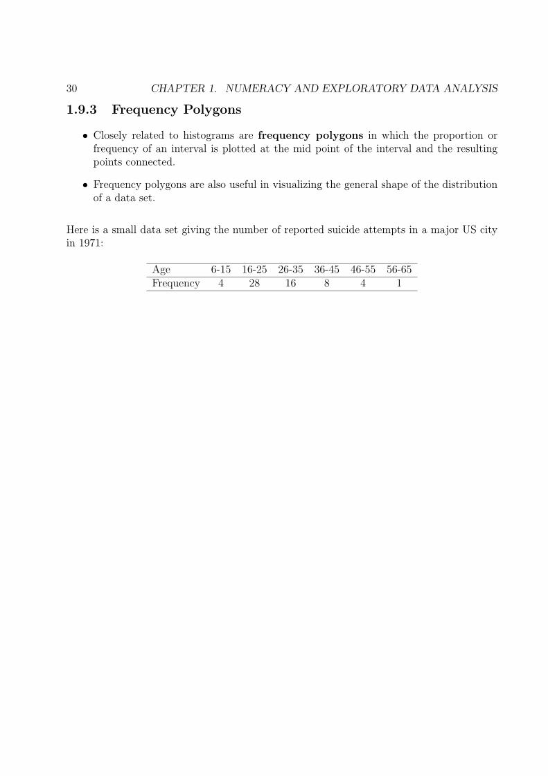
1.9.3 Frequency Polygons
• Closely related to histograms are frequency polygons in which the proportion orfrequency of an interval is plotted at the mid point of the interval and the resultingpoints connected.
• Frequency polygons are also useful in visualizing the general shape of the distributionof a data set.
Here is a small data set giving the number of reported suicide attempts in a major US cityin 1971:
Age 6-15 16-25 26-35 36-45 46-55 56-65Frequency 4 28 16 8 4 1

1.9. BAR PLOTS AND HISTOGRAMS 31
The frequency polygon for this data set is as follows:
Figure 1.7:

32 CHAPTER 1. NUMERACY AND EXPLORATORY DATA ANALYSIS
1.10 Sample Distribution Functions
• Another useful graphical display is the sample distribution function or empiricaldistribution function which is a plot of the proportion of values less than or equalto y versus y where y represents the ordered values of the data set.
• These plots can be conveniently made using current software but usually involve toomuch computation to be done by hand.
• They represent a very valuable technique for comparing observed data sets to theoret-ical models as we will see later.

1.10. SAMPLE DISTRIBUTION FUNCTIONS 33
Here is the sample distribution function for the first data set on ages.
Figure 1.8:

34 CHAPTER 1. NUMERACY AND EXPLORATORY DATA ANALYSIS
1.11 Smoothing
Time series data of the form yt : t = 0, 1, 2, . . . , n which we abbreviate to yt can usefullybe separate d into two additive parts: zt and rt where
• zt is the smooth or signal and represents that part of the data which is slowly varyingand structured.
• rt is the rough or noise and represents that part of the data which is rapidly varyingand unstructured.
zt, the smooth, tells us about long-run patterns while rt, the roughh, tells us aboutexceptional points. The operator which converts the data yt into the smooth is called adata smoother. The smoothed data may then be written as Smyt. The correspondingrough is then given by
Royt = yt − Smyt
There are many smoothers, defined by their properties. For our purposes two generaltypes are important:
• Linear smoothers defined by the property
Smaxt + byt = aSmxt+ bSmyt
• Semi-linear smoothers defined by the property
Smayt + b = aSmyt+ b
Examples of linear smoothers include moving averages e.g.
Smyt =yt−1 + yt + yt+1
3
and weighted moving averages such as Hanning defined by
Smyt =1
4yt−1 +
1
2yt +
1
4yt+1
(Special adjustments are made at the ends of the series.

1.11. SMOOTHING 35
Examples of semi-linear smoothers include running medians of length 3 or 5 when smooth-ing without a computer or even lengths if using a statistical package with the right programs.e.g.
Smyt = medyt−1, yt, yt+1is a smoother of running medians of length 3 with the ends replicated (copied). These kindsof smoothers are applied several times until they “settle down”. Then end adjustments aremade.
The two basic types of smoothers are usually combined to form compound smoothers.The nomenclature for these smoothers is rather bewildering at first but informative: e.g.
3RSSH,twice
refers to the smoother which
• takes running medians of length 3 until the series stabilizes (R)
• the S refers to splitting the repeated values, using the endpoint operator on them andthen replaces the original smooth with these values
• H applies the Hanning smoother to the series which remains
• twice refers to using the smoother on the rough and then adding the rough back to thesmooth to form the final smoothed version
A little trial and error is needed in using these smoothers. Velleman has recommendedthe smoother
4253H,twice
for general use.

36 CHAPTER 1. NUMERACY AND EXPLORATORY DATA ANALYSIS
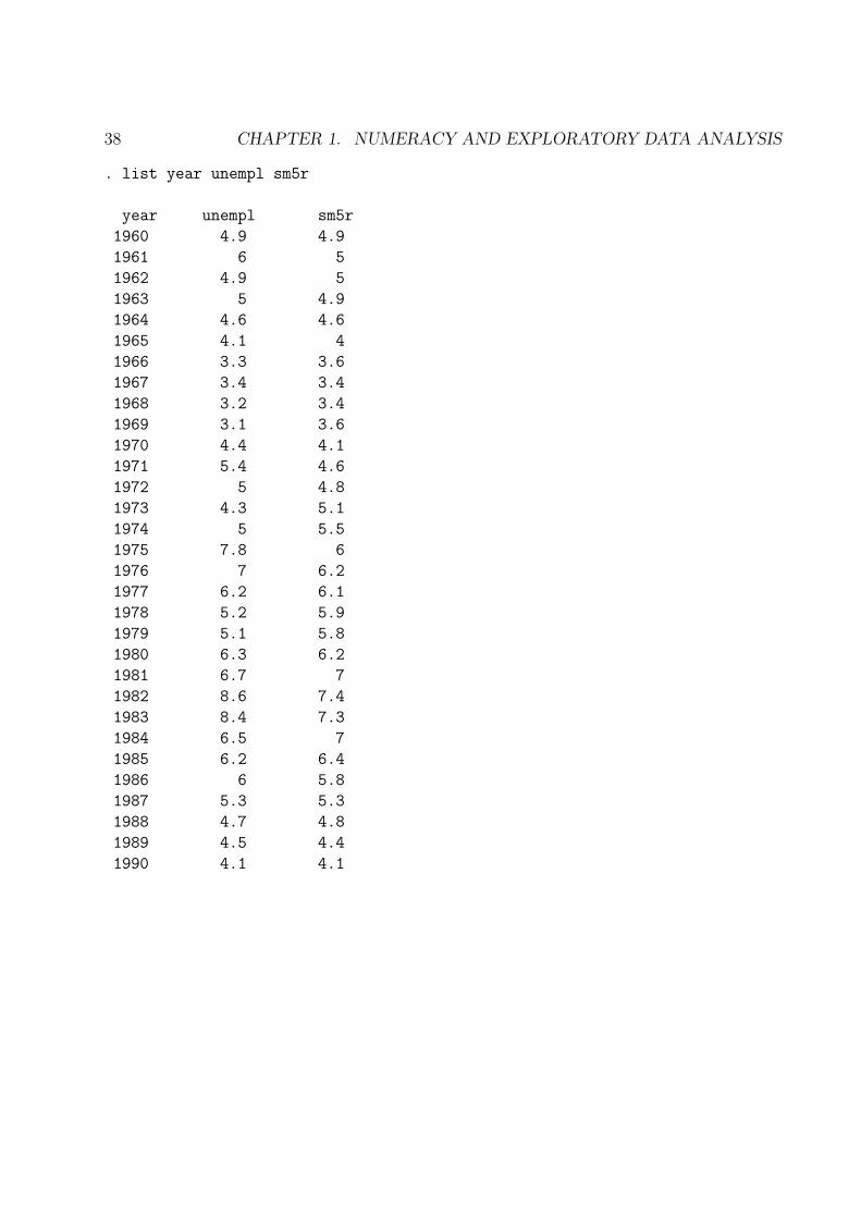
1.11.1 Smoothing Example
To illustrate the smoothing techniques we use data on unemployment percent for the years1960 to 1990.
. infile year unempl using c:\courses\b651201\datasets\unemploy.raw
(31 observations read)
. smooth 3 unempl, gen(sm1)
. smooth 3 sm1, gen(sm2)
. smooth 3R unempl, gen(sm3)
. smooth 3RE unempl, gen(sm4)
. smooth 4253H,twice unempl, gen(sm5)
. gen sm5r=round(sm5,.1)

1.11. SMOOTHING 37
. list year unempl sm1 sm2 sm3 sm4
year unempl sm1 sm2 sm3 sm4
1960 4.9 4.9 4.9 4.9 4.9
1961 6 4.9 4.9 4.9 4.9
1962 4.9 5 4.9 4.9 4.9
1963 5 4.9 4.9 4.9 4.9
1964 4.6 4.6 4.6 4.6 4.6
1965 4.1 4.1 4.1 4.1 4.1
1966 3.3 3.4 3.4 3.4 3.4
1967 3.4 3.3 3.3 3.3 3.3
1968 3.2 3.2 3.2 3.2 3.2
1969 3.1 3.2 3.2 3.2 3.2
1970 4.4 4.4 4.4 4.4 4.4
1971 5.4 5 5 5 5
1972 5 5 5 5 5
1973 4.3 5 5 5 5
1974 5 5 5 5 5
1975 7.8 7 7 7 7
1976 7 7 7 7 7
1977 6.2 6.2 6.2 6.2 6.2
1978 5.2 5.2 5.2 5.2 5.2
1979 5.1 5.2 5.2 5.2 5.2
1980 6.3 6.3 6.3 6.3 6.3
1981 6.7 6.7 6.7 6.7 6.7
1982 8.6 8.4 8.4 8.4 8.4
1983 8.4 8.4 8.4 8.4 8.4
1984 6.5 6.5 6.5 6.5 6.5
1985 6.2 6.2 6.2 6.2 6.2
1986 6 6 6 6 6
1987 5.3 5.3 5.3 5.3 5.3
1988 4.7 4.7 4.7 4.7 4.7
1989 4.5 4.5 4.5 4.5 4.5
1990 4.1 4.1 4.1 4.1 4.1
38 CHAPTER 1. NUMERACY AND EXPLORATORY DATA ANALYSIS
. list year unempl sm5r
year unempl sm5r
1960 4.9 4.9
1961 6 5
1962 4.9 5
1963 5 4.9
1964 4.6 4.6
1965 4.1 4
1966 3.3 3.6
1967 3.4 3.4
1968 3.2 3.4
1969 3.1 3.6
1970 4.4 4.1
1971 5.4 4.6
1972 5 4.8
1973 4.3 5.1
1974 5 5.5
1975 7.8 6
1976 7 6.2
1977 6.2 6.1
1978 5.2 5.9
1979 5.1 5.8
1980 6.3 6.2
1981 6.7 7
1982 8.6 7.4
1983 8.4 7.3
1984 6.5 7
1985 6.2 6.4
1986 6 5.8
1987 5.3 5.3
1988 4.7 4.8
1989 4.5 4.4
1990 4.1 4.1

1.11. SMOOTHING 39
. graph unempl sm4 year,s(oi) c(ll) ti(Unemployment and 3RE Smooth) xlab
. graph unempl sm5r year,s(oi) c(ll) ti(Unemployment and 4253H,twice Smooth) x
> lab
. log close
The graphs on the following two pages show the smoothed versions and the original data.

40 CHAPTER 1. NUMERACY AND EXPLORATORY DATA ANALYSIS
Graph of Unemployment Data and 3RE smooth
Figure 1.9:

1.11. SMOOTHING 41
Graph of Unemployment Data and 4253H,twice Smooth.
Figure 1.10:

42 CHAPTER 1. NUMERACY AND EXPLORATORY DATA ANALYSIS
1.12 Shapes of Batches
Figure 1.11:

1.13. REFERENCES 43
1.13 References
1. Bound, J. A. and A. S. C. Ehrenberg (1989). Significant Sameness. J. R. Statis. Soc.A 152(Part 2): pp. 241-247.
2. Chakrapani, C. Numeracy. Encyclopedia of Statistics.
3. Chambers, J. M., W. S. Cleveland, et al. (1983). Graphical Methods for Data Analysis,Wadsworth International Group.
4. Chatfield, C. (1985). The Initial Examination of Data. J.R.Statist. Soc. A 148(3):214-253.
5. Cleveland, W. S. and R. McGill (1984). The Many Faces of a Scatterplot. JASA79(388): 807-822.
6. Doksum, K. A. (1977). Some Graphical Methods in Statistics. Statistica NeelandicaVol. 31(No. 2): pp. 53-68.
7. Draper, D., J. S. Hodges, et al. (1993). Exchangability and Data Analysis. J. R.Statist. Soc. A 156(Part 1): pp. 9-37.
8. Ehrenberg, A. S. C. (1977). Graphs or Tables ? The Statistician Vol. 27(No.2): pp.87-96.
9. Ehrenberg, A. S. C. (1986). Reading a Table: An Example. Applied Statistics 35(3):237-244.
10. Ehrenberg, A. S. C. (1977). Rudiments of Numeracy. J. R. Statis. Soc. A 140(3):277-297.
11. Ehrenberg, A. S. C. Reduction of Data. Johnson and Kotz.
12. Ehrenberg, A. S. C. (1981). The Problem of Numeracy. American Statistician 35(3):67-71.
13. Finlayson, H. C. The Place of ln x Among the Powers of x. American MathematicalMonthly: 450.
14. Gan, F. F., K. J. Koehler, et al. (1991). Probability Plots and Distribution Curves forAssessing the Fit of Probability Models. American Statistician 45(1): 14-21.

44 CHAPTER 1. NUMERACY AND EXPLORATORY DATA ANALYSIS
15. Goldberg, K. and B. Iglewicz (1992). Bivariate Extensions of the Boxplot. Technomet-rics 34(3): 307-320.
16. Hand, D. J. (1996). Statistics and the Theory of Measurement. J. R. Statist. Soc. A159(Part 3): pp. 445-492.
17. Hand, D. J. (1998). Data Mining: Statistics and More? American Statistics 52(2):112-118.
18. Hoaglin, D. C., F. Mosteller, et al. (1991). Fundamentals of Exploratory Analysis ofVariance, John Wiley & Sons, Inc.
19. Hoaglin, D. C., F. Mosteller, et al., Eds. (1983). Understanding Robust and Ex-ploratory Data Analysis, John Wiley & Sons, Inc.
20. Hunter, J. S. (1988). The Digidot Plot. American Statistician 42(1): 54.
21. Hunter, J. S. (1980). The National System of Scientific Measurement. Science 210:869-874.
22. Kafadar, K. Notched Box-and-Whisker Plots. Encyclopedia of Statistics. Johnson andKotz.
23. Kruskal, W. (1978). Taking Data Seriously. Toward a Metric of Science, John Wiley& Sons: 139-169.
24. Mallows, C. L. and D. Pregibon (1988). Some Principles of Data Analysis, StatisticalResearch Reports No. 54 AT&T Bell Labs.
25. McGill, R., J. W. Tukey, et al. (1978). Variations of Box Plots. American Statistician32(1): 12-16.
26. Mosteller, F. (1977). Assessing Unknown Numbers: Order of Magnitude Estimation.Statistical Methods for Policy Analysis. W. B. Fairley and F. Mosteller, Addison-Wesley.
27. Paulos, J. A. (1988). Innumeracy: Mathematical Illiteracy and Its Consequences, Hilland Wang.
28. Paulos, J. A. (1991). Beyond Numeracy: Ruminations of a Numbers Man, Alfred A.Knopf.

1.13. REFERENCES 45
29. Preece, D. A. (1987). The language of size, quantity and comparison. The Statistician36: 45-54.
30. Rosenbaum, P. R. (1989). Exploratory Plots for Paired Data. American Statistician43(2): 108-109.
31. Scott, D. W. (1979). On optimal and data-based histograms. Biometrika 66(3): pp.605-610.
32. Scott, D. W. (1985). Frequency Polygons: Theory and Applications. JASA 80(390):348-354.
33. Sievers, G. L. Probability Plotting. Encyclopedia of Statistics. Johnson and Kotz:232-237.
34. Snee, R. D. and C. G. Pfeifer.. Graphical Representation of Data. Encyclopedia ofStatistics. Johnson and Kotz: 488-511.
35. Stevens, S. S. (1968). Measurement, Statistics and the Schemapric View. Science161(3844): 849-856.
36. Stirling, W. D. (1982). Enhancements to Aid Interpretation of Probablity Plots. TheStatistician 31(3): 211.
37. Sturges, H. A. (1926). The Choice of Class Interval. JASA 21: 65-66.
38. Terrell, G. R. and D. W. Scott (1985). Oversmoothed Nonparametric Density Esti-mates. JASA 80(389): 209-213.
39. Tukey, J. W. (1980). We Need Both Exploratory and Confirmatory. American Statis-tician 34(1): 23-25.
40. Tukey, J. W. (1986). Sunset Salvo. American Statistician 40(1): 72-76.
41. Tukey, J. W. (1977). Exploratory Data Analysis, Addison Wesley.
42. Tukey, J. W. and C. L. Mallows An Overview of Techniques of Data Analysis, Empha-sizing Its Exploratory Aspects: 111-172.
43. Velleman, P. F. Applied Nonlinear Smoothing. Sociological Methodology 1982 SanFrancisco: Jossey-Bass

46 CHAPTER 1. NUMERACY AND EXPLORATORY DATA ANALYSIS
44. Velleman, P. F. and L. Wilkinson (1993). Nominal, Ordinal, Interval, and Ratio Ty-pologies Are Misleading. American Statistician 47(1): 65-72.
45. Wainer, H. (1997). Improving Tabular Displays, With NAEP Tables as Examples andInspirations. Journal of Educational and Behavioral Statistics 22(1): 1-30.
46. Wand, M. P. (1997). Data-Based Choice of Histogram Bin Width. American Statisti-cian Vol. 51(No. 1): pp. 59-64.
47. Wilk, M. B. and R. Gnanadesikian (1968). Probability plotting methods for the anal-ysis of data. Biometrika 55(1): 1-17.

Chapter 2
Probability
2.1 Mathematical Preliminaries
2.1.1 Sets
To study statistics effectively we need to learn some probability. There are certain elementarymathematical concepts which we use to increase the precision of our discussions. The useof set notation provides a convenient and useful way to be precise about populations andsamples.
Definition: A set is a collection of objects called points or elements.
Examples of sets include:
• set of all individuals in this class
• set of all individuals in Baltimore
• set of integers including 0 i.e. 0, 1, . . .• set of all non-negative numbers i.e. [0, +∞)
• set of all real numbers i.e. (−∞, +∞)
47

48 CHAPTER 2. PROBABILITY
To describe the contents of a set we will follow one of two conventions:
• Convention 1: Write down all of the elements in the set and enclose them in curlybrackets. Thus the set consisting of the four numbers 1, 2, 3 and 4 is written as
1, 2, 3, 4
• Convention 2: Write down a rule which determines or defines which elements are inthe set and enclose the result in curly brackets. Thus the set consisting of the fournumbers 1, 2, 3 and 4 is written as
x : x = 1, 2, 3, 4
and is read as “the set of all x such that x = 1, 2, 3, or 4”. The general convention isthus
x : C(x)and is read as “the set of all x such that the condition C(x) is satisfied”.
Obviously convention 2 is more useful for complicated and large sets.

2.1. MATHEMATICAL PRELIMINARIES 49
Notation and Definitions:
• x ∈ A means that the point x is a point in the set A
• x 6∈ A means that the point x is not a point in the set A Thus1 ∈ 1, 2, 3, 4 but 5 6∈ 1, 2, 3, 4
• A ⊂ B means that each a ∈ A implies that a ∈ B. A. Such an A is said to be asubset of B. Thus1, 2 ⊂ 1, 2, 3, 4
• A = B means that every point in A is also in B and conversely. More precisely A = Bmeans that A ⊂ B and B ⊂ A.
• The union of two sets A and B is denoted by A ∪ B and is the set of all points xwhich are in at least one of the sets. Thus if A = 1, 2 and B = 2, 3, 4 thenA ∪B = 1, 2, 3, 4
• The intersection of two sets A and B is denoted by A∩B and is the set of all points xwhich are in both of the sets. Thus if A = 1, 2 and B = 2, 3, 4 then A∩B = 2.
• If there are no points x which are in both A and B we say that A and B are disjointor mutually exclusive and we write
A ∩B = ∅
where ∅ is called the empty set (the set containing no points).

50 CHAPTER 2. PROBABILITY
• Each set under discussion is usually considered to be a subset of a larger set Ω calledthe sample space.
• The complement of a set A, Ac is the set of all points not in A i.e.
Ac = x : x 6∈ A
Thus if Ω = 1, 2, 3, 4, 5 and A = 1, 2, 4 then Ac = 3, 5.• If B ⊂ A then A−B = A ∩Bc = x : x ∈ A ∩Bc• If a and b are elements or points we call (a, b) an ordered pair. a is called the first
coordinate and b is called the second coordinate. Two ordered pairs are equal definedto be equal if and only if both their first and second coordinates are equal. Thus
(a, b) = (c, d) if and only if a = c and b = d
Thus if we record for an individual their blood pressure and their age the result maybe written as (age, blood pressure).
• The Cartesian product of two sets A and B is written as A × B and is the set ofall ordered pairs having as first coordinate an element of A and second coordinate anelement of B. More precisely
A×B = (a, b) : a ∈ A; b ∈ B
Thus if A = 1, 2, 3 and B = 3, 4 then
A×B = (1, 3), (1, 4), (2, 3), (2, 4), (3, 3), (3, 4)
• Extension of Cartesian products to three or more sets is useful. Thus
A1 × A2 × A3 = (a1, a2, a3) : a1 ∈ A1, a2 ∈ A2, a3 ∈ A3
defines a set of triples. Two triples are equal if and only if they are equal coordinatewise.Most computer based storage systems (data base programs) implicitly use Cartesianproducts to label and store data values.
• An n tuple is an ordered collection of n elements of the form a1, a2, . . . , an.

2.1. MATHEMATICAL PRELIMINARIES 51
example: Consider the set (population) of all individuals in the United States. If
• A is all those who carry the AIDS virus
• B is all homosexuals
• C is all IV drug users
Then
• The set of all individuals who carry the AIDS virus and satisfy only one of the othertwo conditions is
(A ∩B ∩ Cc) ∪ (A ∩Bc ∩ C)
• The set of all individuals satisfying at least two of the conditions is
(A ∩B) ∪ (A ∩ C) ∪ (B ∩ C)
• The set of individuals satisfying exactly two of the conditions is
(A ∩B ∩ Cc) ∪ (A ∩Bc ∩ C) ∪ (Ac ∩B ∩ C)
• The set of all individuals satisfying all three conditions is
A ∩B ∩ C
• The set of all individuals satisfying at least one of the conditions is
A ∪B ∪ C

52 CHAPTER 2. PROBABILITY
2.1.2 Counting
Many probability problems involve “counting the number of ways” something can occur.
Basic Principle of Counting: Given two sets A and B with n1 and n2 elements respec-tively of the form
A = a1, a2, . . . , an1B = b1, b2, . . . , bn2
then the set A×B consisting of all ordered pairs of the form (ai, bj) contains n1n2 elements.
• To see this consider the table
b1 b2 · · · bn2
a1 (a1, b1) a1, b2) · · · (a1, bn2)a2 (a2, b1) a2, b2) · · · (a2, bn2)...
......
. . ....
an1 (an1 , b1) an1 , b2) · · · (an1 , bn2)
The conclusion is thus obvious.
• Equivalently: If there are n1 ways to perform operation 1 and n2 ways to performoperation 2 then there are n1n2 ways to perform first operation 1 and then operation2.
• In general if there are r operations in which the ith operation can be performed in ni
ways then there are n1n2 · · ·nr ways to perform the r operations in sequence.
• Permutations: If a set S contains n elements, there are
n! = n× (n− 1)× · · · × 3× 2× 1
different n tuples which can be formed from the n elements of S.
– By convention 0! = 1.
– If r ≤ n there are
(n)r = (n− r + 1)(n− r + 2) · · · (n− 1)n
r tuples composed of elements of S.
2.1. MATHEMATICAL PRELIMINARIES 53
• Combinations: If a set S contains n elements and r ≤ n, there are
Cnr =
(n
r
)=
n!
r!(n− r)!
subsets of size r containing elements of S.
To see this we note that if we have a subset of size r from S there are r! permutationsof its elements, each of which is an r tuple of elements from S. Therefore we have theequation
r! Cnr = (n)r
and the conclusion follows.
examples:
(1) For an ordinary deck of 52 cards there are 52 × 51 × 50 ways to choose a “hand” ofthree cards.
(2) If we toss two dies (each six-sided with sides numbered 1-6) there are 36 possibleoutcomes.
(3) The use of the convention that 0! = 1 can be considered a special case of the Gammafunction defined by
Γ(α) =∫ ∞
0xα−1e−xdx
defined for any positive α. We note by integration by parts that
Γ(α) = (α− 1)xα−1
∣∣∣∣∣∞
0
+ (α− 1)∫ ∞
0xα−2e−xdx = (α− 1)Γ(α− 1)
It follows that if α = n where n is an integer then
Γ(n) = (n− 1)!
and hence with n = 10! = Γ(1) =
∫ ∞
0e−xdx = 1

54 CHAPTER 2. PROBABILITY
2.2 Relating Probability to Responses and Populations
Probability is a measure of the uncertainty associated with the occurrence of events.
• In applications to statistics probability is used to model the uncertainty associatedwith the response of a study.
• Using probability models and observed responses (data) we make statements (statisticalinferences) about the study:
The probability model allows us to relate the uncertainty associated with sampleresults to statements about population characteristics.
Without such models we can say little about the population and virtually nothingabout the reliability or generalizability of our results.
• The term experiment or statistical experiment or random experiment denotesthe performance of an observational study, a census or sample survey or a designedexperiment.
The collection, Ω, of all possible results of an experiment will be called the samplespace.
A particular result of an experiment will be called an elementary event anddenoted by ω.
An event is a collection of elementary events.
Events are thus sets of elementary events.

2.2. RELATING PROBABILITY TO RESPONSES AND POPULATIONS 55
• Notation and interpretations:
ω ∈ E means that E occurs when ω occurs
ω 6∈ E means that E does not occur when ω occurs
E ⊂ F means that the occurrence of E implies the occurrence of F
E ∩ F means the event that both E and F occur
E ∪ F means the event that at least one of E or F occur
φ denotes the impossible event
E ∩ F = φ means that E and F are mutually exclusive
Ec is the event that E does not occur
Ω is the sample space

56 CHAPTER 2. PROBABILITY
2.3 Probability and Odds - Basic Definitions
2.3.1 Probability
Definition: Probability is an assignment to each event of a number called its probabilitysuch that the following three conditions are satisfied:
(1) P (Ω) = 1 i.e. the probability assigned to the certain event or sample space is 1
(2) 0 ≤ P (E) ≤ 1 for any event E i.e. the probability assigned to any event must bebetween 0 and 1
(3) If E1 and E2 are mutually exclusive then
P (E1 ∪ E2) = P (E1) + P (E2)
i.e. the probability assigned to the union of mutually exclusive events equals the sumof the probabilities assigned to the individual events.
P (E) is called the probability of the event E
Note: In considering probabilities for continuous responses we need a stronger form of (3):
P (∪iEi) =∑
i
P (Ei)
for any countable collection of events which are mutually exclusive.

2.3. PROBABILITY AND ODDS - BASIC DEFINITIONS 57
2.3.2 Properties of Probability
Important properties of probabilities are:
• P (Ec) = 1− P (E)
• P (∅) = 0
• E1 ⊂ E2 implies P (E1) ≤ P (E2)
• P (E1 ∪ E2) = P (E1) + P (E2)− P (E1 ∩ E2)
Rather than develop the theory of probability we will:
• Develop the most important probability models used in statistics.
• Learn to use these models to make calculations according to the definitions and prop-erties listed above
• Learn how to interpret probabilities.
examples:
• Suppose that P (A) = .4, P (B) = .3 and P (A ∩B) = .2 then
P (A ∪B) = .4 + .3− .2 = .5
• For any three events A,B and C we have
P (A∪B∪C) = P (A)+P (B)+P (C)−P (A∩B)−P (A∩C)−P (B∩C)+P (A∩B∩C)
and henceP (A ∪B ∪ C) ≤ P (A) + P (B) + P (C)

58 CHAPTER 2. PROBABILITY
2.3.3 Methods for Obtaining Probability Models
The four most important sample spaces for statistical applications are
0, 1, 2, . . . , n (discrete-finite)
0, 1, 2, . . . (discrete-countable)
[0,∞) (continuous)
(−∞,∞) (continuous)
For these sample spaces probabilities are defined by probability mass functions (discretecase) and probability density functions (continuous case). We shall call both of these prob-ability density functions (pdfs).
For the discrete cases a pdf assigns a number f(x) to each x in the sample space suchthat
f(x) ≥ 0 and∑x
f(x) = 1
Then P (E) is defined byP (E) =
∑
x∈E
f(x)
For the continuous cases a pdf assigns a number f(x) to each x in the sample spacesuch that
f(x) ≥ 0 and∫
xf(x)dx = 1
Then P (E) is defined by
P (E) =∫
x∈Ef(x)dx
Since sums and integrals over disjoint sets are additive probabilities can be assigned usingpdfs (i.e. the probabilities so assigned obey the three axioms of probabilities).
examples:
If
f(x) =
(n
x
)px(1− p)n−x x = 0, 1, 2, . . . , n

2.3. PROBABILITY AND ODDS - BASIC DEFINITIONS 59
where 0 ≤ p ≤ 1 we have a binomial probabilty model with parameter p. The fact that
∑x
f(x) =n∑
x=0
(n
x
)px(1− p)n−x = 1
follows from the fact (Newton’s binomial expansion) that
(a + b) =n∑
x=0
(n
x
)axbn−x
for any a and b.
If
f(x) =λxe−λ
x!x = 0, 1, 2, . . .
where λ ≥ 0 we have a Poisson probability model with parameter λ. The fact that
∑x
f(x) =∞∑
x=0
λxe−λ
x!= 1
follows from the fact that ∞∑
x=0
λx
x!= eλ
Iff(x) = λe−λx 0 ≤ x < ∞)
where λ ≥ 0 we have an exponential probability model with parameter λ. The factthat ∫
xf(x)dx =
∫ ∞
0λe−λxdx = 1
follows from the fact that ∫ ∞
0e−λxdx =
1
λ
60 CHAPTER 2. PROBABILITY
Iff(x) = (2πσ)−1/2 exp−(x− µ)2/2σ2 −∞ < x < +∞
where −∞ < µ < +∞ and σ > 0 we have a normal or Gaussian probability modelwith parameters µ and σ2. The fact that
∫
xf(x)dx =
∫ +∞
−∞(2πσ)−1/2 exp−(x− µ)2/2σ2dx = 1
is shown in the supplemental notes.
Each of the above examples of probability models play major roles in the statisticalanalysis of data from experimental studies. The binomial is used to model prospective(cohort), retrospective (case-control) studies in epeidemiology, the Poisson is used to modelaccident data, the exponential is used to model failure time data and the normal distributionis used for measurement data which has a bell-shaped distribution as well as to approximatethe binomial and Poisson. The normal distribution also figures in the calculation of manycommon statistics used for inference via the Central Limit Theorem. All of these models arespecial cases of the exponential family of distributions defined as having pdfs of the form:
f(x; θ1, θ2, . . . , θp) = C(θ1, θ2, . . . , θp)h(x) exp
p∑
j=1
tj(x)qj(θ)
2.3. PROBABILITY AND ODDS - BASIC DEFINITIONS 61
2.3.4 Odds
Closely related to probabilities are odds.
• If the odds of an event E occurring are given as a to b this means, by definition, that
P (E)
P (Ec)=
P (E)
1− P (E)=
a
b
We can solve for P (E) to obtain
P (E) =a
a + b
Thus we can go from odds to probabilities and vice-versa.
Thinking about probabilities in terms of odds sometimes provides useful interpre-tation of probability statements.
• Odds can also be given as the odds against E are c to d. This means that
P (Ec)
P (E)=
1− P (E)
P (E)=
c
d
so that in this case
P (E) =d
c + d
• example: The odds against disease 1 are 9 to 1. Thus
P (disease 1) =1
1 + 9= .1
• example: The odds of thundershowers this afternoon are 2 to 3. Thus
P (thundershowers) =2
2 + 3= .4

62 CHAPTER 2. PROBABILITY
• Ratios of odds are called odds ratios and play an important role in modern epidemi-ology where they are used to quantify the risk associated with exposure.
example: Let OR be the odds ratio for the occurrence of a disease in an exposedpopulation relative to an unexposed or control population. Thus
OR =odds of disease in exposed population
odds of disease in control population=
p2
1−p2
p1
1−p1
where p2 is the probability of the disease in the exposed population and p1 is theprobability of the disease in the control population.
Note that if OR = 1 then
p2
1− p2
=p1
1− p1
which implies that p2 = p1 i.e. that the probability of disease is the same in theexposed and control population.
If OR > 1 thenp2
1− p2
>p1
1− p1
which can be shown to imply that p2 > p1 i.e. that the probability of diseasein the exposed population exceeds the probability of the disease in the controlpopulation.
If OR < 1 the reverse conclusion holds i.e. the probability of disease in the controlpopulation exceeds the probability of disease in the exposed population.

2.3. PROBABILITY AND ODDS - BASIC DEFINITIONS 63
• The odds ratio, while useful in comparing the relative magnitude of risk of diseasedoes not convey the absolute magnitude of the risk (unless the risk is small).
Note thatp2
1−p2
p1
1−p1
= OR
implies that
p2 = OR
[p1
1 + (OR− 1)p1
]
Consider a situation in which the odds ratio is 100 for exposed vs control. Thusif OR = 100 and p1 = 10−6 (one in a million) then p2 is approximately 10−4 (onein ten thousand). If p1 = 10−2 (one in a hundred) then
p2 = 100
1100
1 + 99(
1100
) =
100
199= .50
64 CHAPTER 2. PROBABILITY
2.4 Interpretations of Probability
Philosophers have discussed for several centuries at various levels what constitues “proba-bility”. For our purposes probability has three useful operational interpretations.
2.4.1 Equally Likely Interpretation
Consider an experiment where the sample space consists of a finite number of elementaryevents
e1, e2, . . . , eN
If, before the experiment is performed, we consider each of the elementary events to be“equally likely” or exchangeable then an assignment of probability is given by
p(ei) =1
N
This allows an interpretation of statements such as “we selected an individual at randomfrom a population” since in ordinary language at random means that each invidual has thesame chance of being selected. Although defining probability via this recipe is circular it isa useful interpretation in any situation where the sample space is finite and the elementaryevents are deemed equally likely. It forms the basis of much of sample survey theory wherewe select individuals at random from a population in order to investigate properties of thepopulation.
Summary: The equally likely interpretation assumes that each element in the samplespace has the same chance of occuring.
2.4. INTERPRETATIONS OF PROBABILITY 65
2.4.2 Relative Frequency Interpretation
Another interpretation of probability is the so called relative frequency interpretation.
• Imagine a long series of trials in which the event of interest either occurs or does notoccur.
• The relative frequency (number of trials in which the event occurs divided by the totalnumber of trials) of the event in this long series of trials is taken to be the probabilityof the event.
• This interpretation of probability is the most widely used interpretation in scientificstudies. Note, however, that it is also circular.
• It is often called the “long run frequency interpretation”.
2.4.3 Subjective Probability Interpretation
This interpretation of probability requires the personal evaluation of probabilities using in-difference between two wagers (bets).
Suppose that you are interested in determining the probability of an event E. Considertwo wagers defined as follows:
Wager 1 : You receive $100 if the event E occurs and nothing if it does not occur.
Wager 2 : There is a jar containing x white balls and N − x red balls. You receive $100 ifa white ball is drawn and nothing otherwise.
You are required to make one of the two wagers. Your probability of E is taken to bethe ratio x/N at which you are indifferent between the two wagers.
66 CHAPTER 2. PROBABILITY
2.4.4 Does it Matter?
• For most applications of probability in modern statistics the specific interpretation ofprobability does not matter all that much.
• What matters is that probabilities have the properties given in the definition and thoseproperties derived from them.
• In this course we will take probability as a primitive concept leaving it to philosophersto argue the merits of particular interpretations.
• Each of the interpretations discussed above satisfies the three basic axioms of thedefinition of probability.

2.5. CONDITIONAL PROBABILITY 67
2.5 Conditional Probability
• Conditional probabilities possess all the properties of probabilities.
• Conditional probabilities provide a method to revise probabilities in the light of addi-tional information (the process itself is called conditioning).
• Conditional probabilities are important because almost all probabilities are conditionalprobabilities.
example:Suppose a coin is flipped twice and you are told that at least one coin is a head. What isthe chance or probability that they are both heads? Assuming a fair coin and a good tosseach of the four possibilities
(H,H), (H, T ), (T, H), (T, T )
which constitutes the sample space for this experiment has the same probability i.e. 1/4.Since the information given rules out (T, T ); a logical answer for the conditional probabilityof two heads given at least one head is 1/3.
example:A family has three children. What is the probability that two of the children are boys?Assuming that gender distributions are equally likely the eight equally likely possibilitiesare:
(B, B, B), (B, B, G), (B, G,B), (G,B,B),
(G,G, B), (G,B, G), (B, G, G), (G,G, G)
Thus the probability of two boys is
1
8+
1
8+
1
8=
3
8
Depending on the conditioning information the probability of two boys is modified e.g.
• What is the probability of two boys if you are told that at least one child in the familyis a boy?Answer: 3
7

68 CHAPTER 2. PROBABILITY
• What is the probability of two boys if you are told that at least one child in the familyis a girl?Answer: 3
7
• What is the probability of two boys if you are told that the oldest child is a boy?Answer: 1
2
• What is the probability of two boys if you are told that the oldest child is a girl?Answer: 1
4
We generalize to other situations using the following definition:
Definition: The conditional probability of event B given event A is
P (B|A) =P (B ∩ A)
P (A)
provided that P (A) > 0
example: The probability of two boys given that the oldest child is a boy is the probabilityof the event “two boys in the family and the oldest child in the family is a boy” dividedby the probability of the event “the oldest child in the family is a boy”. Thus the requiredconditional probability is given by
P ((B, G, B), (G,B,B))P ((B,B,B), (B,G, B), (G, B, B), (G,G, B)) =
2848
=1
2

2.5. CONDITIONAL PROBABILITY 69
2.5.1 Multiplication Rule
The multiplication rule for probabilities is as follows:
P (A ∩B) = P (A)P (B|A)
which can immediately be extended to
P (A ∩B ∩ C) = P (A)P (B|A)P (C|A ∩B)
and in general to:
P (E1 ∩ E2 ∩ · · · ∩ En) = P (E1)P (E2|E1) · · ·P (En|E1 ∩ E2 ∩ · · · ∩ En−1)
example: There are n people in a room. What is the probability that at least two of thepeople have a common birthday?
Solution: We first note that
P (common birthday) = 1− P (no common birthday)
If there are just two people in the room then
P (no common birthday) =(
365
365
) (364
365
)
while for three people we have
P (no common birthday) =(
365
365
) (364
365
) (363
365
)
It follows that the probability of no common birthday with n people in the room is givenby (
365
365
) (364
365
)· · ·
(365− (n− 1)
365
)

70 CHAPTER 2. PROBABILITY
Simple calculations show that if n = 23 then the probability of no common birthday isslightly less than 1
2. Thus if the number of people in a room is 23 or larger the probability of
a common birthday exceeds 12. The following is a short table of the results for other values
of n
n Prob n Prob2 .003 17 .3153 .008 18 .3474 .016 19 .3795 .027 20 .4116 .041 21 .4447 .056 22 .4768 .074 23 .5079 .095 24 .538
10 .117 25 .56911 .141 26 .59812 .167 27 .62713 .194 28 .65414 .223 29 .68115 .253 30 .70616 .284 31 .730
2.5. CONDITIONAL PROBABILITY 71
2.5.2 Law of Total Probability
Law of Total Probability:For any event E we have
P (E) =∑
i
P (E|Ei)P (Ei)
where Ei is a partition of the sample space i.e. the Ei are mutually exclusive and theirunion is the sample space.
example: An examination consists of multiple choice questions. Each question is a multiplechoice question in which there are 5 alternative answers only one of which is correct. If astudent has diligently done his or her homework he or she is certain to select the correctanswer. If not he or she has only a one in five chance of selecting the correct answer (i.e.they choose an answer at random). Let
• p be the probability that the student does their homework
• A the event that they do their homework
• B the event that they select the correct answer

72 CHAPTER 2. PROBABILITY
(i) What is the probability that the student selects the correct answer to a question?
Solution: We are given
P (A) = p ; P (B|A) = 1 and P (B|Ac) =1
5
By the Law of Total Probability
P (B) = P (A)P (B|A) + P (Ac)P (B|Ac)
= p× 1 + (1− p)×(
1
5
)
=5p + 1− p
5
=4p + 1
5
(ii) What is the probability that the student did his or her homework given that theyselected the correct anwer to the question?
Solution: In this case we want P (A|B) so that
P (A|B) =P (A ∩B)
P (B)
=P (A)P (B|A)
P (B)
=1× p4p+1
5
=5p
4p + 1

2.5. CONDITIONAL PROBABILITY 73
example: Cross-Sectional Study
Suppose a population of individuals is classified into four categories defined by
• their disease status (D is diseased and Dc is not diseased)
• their exposure status (E is exposed and Ec is not exposed).
If we observe a sample of n individuals so classified we have the following populationprobabilities and observed data.
Population SampleProbabilities Numbers
Dc D Total Dc D TotalEc P (Ec, Dc) P (Ec, D) P (Ec) n(Ec, Dc) n(Ec, D) n(Ec)E P (E, Dc) P (E, D) P (E) n(E,Dc) n(E, D) n(E)
Total P (Dc) P (D) 1 n(Dc) n(D) n
The law of total probability then states that
P (D) = P (E, D) + P (Ec, D)
= P (D|E)P (E) + P (D|Ec)P (Ec)

74 CHAPTER 2. PROBABILITY
Define the following quantities:
Population Parameters Sample Estimatesprob of exposure prob of exposure
P (E) = P (E, D) + P (E, Dc) p(E) = n(E,D)+n(E,Dc)n
prob of disease given exposed prob of disease given exposed
P (D|E) = P (E,D)P (E)
p(D|E) = n(D,E)n(E)
odds of disease if exposed odds of disease if exposed
O(D|E) = P (D,E)P (Dc,E)
o(D|E) = n(D,E)n(Dc,E)
odds of disease if not exposed odds of disease if not exposed
O(D|Ec) = P (D,Ec)P (Dc,Ec)
o(D|Ec) = n(D,Ec)n(Dc,Ec)
odds ratio (relative odds) odds ratio (relative odds)
OR = O(D|E)O(D|Ec)
or = o(D|E)o(D|Ec)
relative risk relative risk
RR = P (D|E)P (D|Ec)
rr = p(D|E)p(D|Ec)
It can be shown that if the disease is rare in both the exposed group and the non exposedgroup then
OR ≈ RR
The above population parameters are fundamental to the epidemiological approach tothe study of disease as it relates to exposure.
example: In demography the crude death rate is defined as
CDR =Total Deaths
Population Size=
D
N
If the population is divided into k age groups or other strata defined by gender, ethnicity,etc. then D = D1 + D2 + · · ·+ Dk and N = N1 + N2 + · · ·+ Nk and hence
CR =D
N=
∑ki=1 Di
N=
∑ki=1 NiMi
N=
k∑
i=1
piMi
where Mi = Di/Ni is the age specfic death rate for the ith age group and pi = Ni/N is theproportion of the population in the ith age group. This is directly analogous to the law oftotal probability,

2.6. BAYES THEOREM 75
2.6 Bayes Theorem
Bayes theorem combines the definition of conditional probability, the multiplication rule andthe law of total probability and asserts that
P (Ei|E) =P (Ei)P (E|Ei)∑j P (Ej)P (E|Ej)
• where E is any event
• the Ej constitute a partition of the sample space
• Ei is any event in the partition.
Since
P (Ei|E) =P (Ei ∩ E)
P (E)
P (Ei ∩ E) = P (Ei)P (E|Ei)
P (E) =∑
j
P (Ej)P (E|Ej)
Bayes theorm is obviously true.
Note: A partition of the sample space is a collection of mutually exclusive events such thattheir union is the sample space.

76 CHAPTER 2. PROBABILITY
example: The probability of disease given exposure is .5 while the probability of diseasegiven non-exposure is .1. Suppose that 10% of the population is exposed. If a diseasedindividual is detected what is the probability that the individual was exposed?
Solution: By Bayes theorem
P (Ex|Dis) =P (Ex)P (Dis|Ex)
P (Ex)P (Dis|Ex) + P (No Ex)P (Dis|No Ex)
=(.1)(.5)
(.1)(.5) + (.9)(.1)
=5
5 + 9
=5
14
The intuitive explanation for this result is as follows:
• Given 1,000 individuals 100 will be exposed and 900 not exposed
• Of the 100 individuals exposed 50 will have the disease.
• of the 900 non exposed individuals 90 will have the disease
Thus of the 140 individuals with the disease, 50 will have been exposed which yields aproportion of 5
14.

2.6. BAYES THEOREM 77
example: Diagnostic Tests
In this type of study we are interested in the performance of a diagnostic test designedto determine whether a person has a disease. The test has two possible results:
• + positive test (the test indicates presence of disease).
• − negative test (the test does not indicate presence of disease).
We thus have the following setup:
Population SampleProbabilities NumbersDc D Total Dc D Total
− P (−, Dc) P (−, D) P (−) n(−, Dc) n(−, D) n(−)+ P (+, Dc) P (+, D) P (+) n(+, Dc) n(+, D) n(+)
Total P (Dc) P (D) 1 n(Dc) n(D) n
78 CHAPTER 2. PROBABILITY
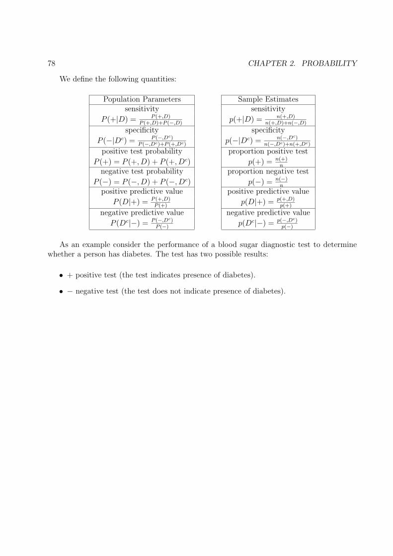
We define the following quantities:
Population Parameters Sample Estimatessensitivity sensitivity
P (+|D) = P (+,D)P (+,D)+P (−,D)
p(+|D) = n(+,D)n(+,D)+n(−,D)
specificity specificity
P (−|Dc) = P (−,Dc)P (−,Dc)+P (+,Dc)
p(−|Dc) = n(−,Dc)n(−,Dc)+n(+,Dc)
positive test probability proportion positive test
P (+) = P (+, D) + P (+, Dc) p(+) = n(+)n
negative test probability proportion negative test
P (−) = P (−, D) + P (−, Dc) p(−) = n(−)n
positive predictive value positive predictive value
P (D|+) = P (+,D)P (+)
p(D|+) = p(+,D)p(+)
negative predictive value negative predictive value
P (Dc|−) = P (−,Dc)P (−)
p(Dc|−) = p(−,Dc)p(−)
As an example consider the performance of a blood sugar diagnostic test to determinewhether a person has diabetes. The test has two possible results:
• + positive test (the test indicates presence of diabetes).
• − negative test (the test does not indicate presence of diabetes).

2.6. BAYES THEOREM 79
The following numerical example is from Epidemiology (1996) Gordis, L. W. B. Saunders.We have the following setup:
Population SampleProbabilities NumbersDc D Total Dc D Total
− P (−, Dc) P (−, D) P (−) 7600 150 7750+ P (+, Dc) P (+, D) P (+) 1900 350 2250
Total P (Dc) P (D) 1 9500 500 10, 000
We calculate the following quantities:
Population Parameters Sample Estimatessensitivity sensitivity
P (+|D) = P (+,D)P (+,D)+P (−,D)
p(+|D) = 350500
= .70
specificity specificity
P (−|Dc) = P (−,Dc)P (−,Dc)+P (+,Dc)
p(−|Dc) = 76009500
= .80
positive test probability proportion positive testP (+) = P (+, D) + P (+, Dc) p(+) = 2250
10,000= .225
negative test probability proportion negative testP (−) = P (−, D) + P (−, Dc) p(−) = 7750
10,000= .775
positive predictive value positive predictive value
P (D|+) = P (+,D)P (+)
p(D|+) = 3502250
= 0.156
negative predictive value negative predictive value
P (Dc|−) = P (−,Dc)P (−)
p(Dc|−) = 76007750
= 0.98

80 CHAPTER 2. PROBABILITY
2.7 Independence
Closely related to the concept of conditional probability is the concept of independence ofevents.
Definition Events A and B are said to be independent if
P (B|A) = P (B)
Thus knowledge of the occurrence of A does not influence the assignment of probabilities toB.
Since
P (B|A) =P (A ∩B)
P (A)
it follows that if A and B are independent then
P (A ∩B) = P (A)P (B)
This last formulation of independence is the definition used in building probability mod-els.

2.8. BERNOULLI TRIAL MODELS; THE BINOMIAL DISTRIBUTION 81
2.8 Bernoulli trial models; the binomial distribution
• One of the most important probability models is the binomial. It is widely used inepidemiology and throughout statistics.
• The binomial model is based on the assumption of Bernoulli trials.
The assumptions for a Bernoulli trial model are
(1) The result of the experiment or study can be thought of as the result of n smallerexperiments called trials each of which has only two possible outcomes e.g. (dead,alive), (diseased, non-diseased), (success, failure)
(2) The outcomes of the trials are independent
(3) The probabilities of the outcomes of the trials remain the same from trial to trial(homogeneous probabilities).
example 1: A group of n individuals are tested to see if they have elevated levels ofcholestrol. Assuming the results are recorded as elevated or not elevated and we can justify(2) and (3) we may apply the Bernoulli trial model.
example 2: A population of n individuals is found to have d deaths during a given periodof time. Assuming we can justify (2) and (3) we may use the Bernoulli model to describethe results of the study.
In Bernoulli trial models the quantity of interest is the number of successes x whichoccur in the n trials. It can be be shown that the following formula gives the probability ofobtaining x successes in n Bernoulli trials
P (x) =
(n
x
)px(1− p)n−x
where
• x can be 0, 1, 2, . . . , n
• p is the probability of success on a given trial

82 CHAPTER 2. PROBABILITY
•(
nx
), read as ”n choose x”, is defined by
(n
x
)=
n!
x! (n− x)!
In this last formula r! = r(r − 1)(r − 2) · · · 3 · 2 · 1 for any integer r and 0! = 1.
Note: The term distribution is used because the formula describes how to distribute prob-ability over the possible values of x.
example: The chance or probability of having an elevated cholesterol level is 1/100. If 10individuals are examined, what is the probability that one or more of them will have beenexposed?
Solution: The binomial model applies so that
P (0) =
(10
0
)(.01)0(1− .01)10−0
= (.99)10
Thus
P (1 or more elevated) = 1− P (0 elevated)
= 1− (.99)10
= .059

2.9. PARAMETERS AND RANDOM SAMPLING 83
2.9 Parameters and Random Sampling
• The numbers n and p which appear in the formula for the binomial distribution areexamples of what statisticians call parameters.
• Different values of n and p give different assignments of probabilities each of the bino-mial type.
• Thus a parameter can be considered as a label which identifies the particular assign-ment of probabilities.
• In applications of the binomial distribution the parameter n is known and can be fixedby the investigator - it is thus a study design parameter.
• The parameter p, on the other hand, is unknown and obtaining information about itis the reason for performing the experiment.
We use the observed data and the model to tell us something about p. This same set-upapplies in most applications of statistics.
To summarize:
• Probability distributions relate observed data to parameters.
• Statistical methods use data and probability models to make statementsabout the parameters of interest.
In the case of the binomial the parameter of interest is p, the probability of success on agiven trial.

84 CHAPTER 2. PROBABILITY
example: Random sampling and the binomial distribution. In many circumstances we aregiven the results of a survey or study in which the investigators state that they examined a“random sample” from the population of interest.
Suppose we have a population containing N individuals or objects. We are presentedwith a “random sample” consisting of n individuals from the population. What does thismean? We begin by defining what we mean by a sample.
Definition: A sample of size n from a target population T containing N objects is anordered collection of n objects each of which is an object in the target population.
In set notation a sample is just an n-tuple with each coordinate being an element of thetarget population. In symbols then a sample s is
s = (a1, a2, . . . , an)
where a1 ∈ T, a2 ∈ T, . . . , an ∈ T .
Specific example:If T = a, b, c, d then a possible sample of size 2 is (a, b) while some others are (b, a) and(c, d). What about (a, a)? Clearly, this is a sample according to the definition.
To distinguish between these two types of samples:
• A sample is taken with replacement if an element in the population can appearmore than once in the sample
• A sample is taken without replacement if an element in the population can appearat most once in the sample.

2.9. PARAMETERS AND RANDOM SAMPLING 85
Thus in our example the possible samples of size 2 with replacement are
(a, a) (a, b) (a, c) (a, d)(b, a) (b, b) (b, c) (b, d)(c, a) (c, b) (c, c) (c, d)(d, a) (d, b) (d, c) (d, d)
while without replacement the possible samples are
(a, b) (a, c) (a, d)(b, a) (c, a) (d, a)(b, c) (c, b) (b, d)(d, b) (c, d) (d, c)
Definition: A random sample of size n from a population of size N is a sample which isselected such that each sample has the same chance of being selected i.e.
P (sample selected) =1
number of possible samples
Thus in the example each sample with replacement would be assigned a chance of 116
whileeach sample without replacement would be assigned a chance of 1
12for random sampling.

86 CHAPTER 2. PROBABILITY
In the general case,
• For sampling with replacement the probability assigned to each sample is
1
Nn
• For sampling without replacement the probability assigned to each sample is
1
(N)n
where (N)n is given by:
(N)n = N(N − 1)(N − 2) · · · (N − n + 1)
In our example we see that
Nn = 42 = 16 and (N)n = (4)2 = 4(4− 2 + 1) = 4× 3 = 12
To summarize: A random sample is the result of a selection process in whicheach sample has the same chance of being selected.

2.9. PARAMETERS AND RANDOM SAMPLING 87
Suppose now that each object in the population can be classified into one of two categoriese.g. (exposed, not exposed), (success, failure), (A, not A), (0, 1) etc. For definiteness let uscall the two outcomes success and failure and denote them by S and F .
In the example suppose that a and b are successes while c and d are failures. The targetpopulation is now
T = a(S), b(S), c(F ), d(F )In general D of the objects will be successes and N −D will be failures.
The question of interest is: If we select a random sample of size n from a population ofsize N consisting of D successes and N −D failures, what is the probability that x successeswill be observed in the sample?
In the example we see that with replacement the samples are
(a(S), a(S)) (a(S), b(S)) (a(S), c(F )) (a(S), d(F ))(b(S), a(S)) (b(S), b(S)) (b(S), c(F )) (b(S), d(F ))(c(F ), a(S)) (c(F ), b(S)) (c(F ), c(F )) (c(F ), d(F ))(d(F ), a(S)) (d(F ), b(S)) (d(F ), c(F )) (d(F ), d(F ))
Thus if sampling is at random with replacement the probabilities of 0 successes, 1 successand 2 successes are given by
P (0) =4
16
P (1) =8
16
P (2) =4
16
If sampling is at random without replacement the probabilities are given by
P (0) =2
12
P (1) =8
12
P (2) =2
12

88 CHAPTER 2. PROBABILITY
These probabilities can, in the general case, be shown to be
without replacement :
P (x successes) =
(n
x
)(D)x(N −D)n−x
(N)n
with replacement :
P (x successes) =
(n
x
) (D
N
)x (1− D
N
)n−x
The distribution without replacement is called the hypergeometric distribution withparameters N, n and D. The distribution with replacement is the binomial distribution withparameters n and p = D/N .
In many applications the sample size, n, is small relative to the population size N . Inthis situation it can be shown that the formula
(n
x
) (D
N
)x (1− D
N
)n−x
provides an adequate approximation to the probabilities for sampling without replacement.
Thus for most applications, random sampling from a population in which each individualis classified as a success or a failure results in a binomial distribution for the probability ofobtaining x successes in the sample.
The interpretation of the parameter p = DN
is thus:
• “the proportion of successes in the target population”
• “the chance that an individual selected at random will be classified as a success”.

2.9. PARAMETERS AND RANDOM SAMPLING 89
example: Prospective (Cohort) Study
In this type of study
• we observe n(E) individuals who are exposed and n(Ec) individuals who are not ex-posed.
• These individuals are followed and the number in each group who develop the diseaseare recorded.
We thus have the following setup:
Population SampleProbabilities Numbers
Dc D Total Dc D TotalEc P (Dc|Ec) P (D|Ec) 1 n(Dc, Ec) n(D, Ec) n(Ec)E P (Dc|E) P (D|E) 1 n(Dc, E) n(D, E) n(E)
We can model this situation as two independent binomial distributions as follows:
n(D,E) is binomial (n(E), P (D|E))
n(D, Ec) is binomial (n(Ec), P (D|Ec))
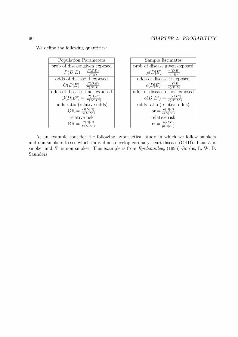
90 CHAPTER 2. PROBABILITY
We define the following quantities:
Population Parameters Sample Estimatesprob of disease given exposed prob of disease given exposed
P (D|E) = P (E,D)P (E)
p(D|E) = n(D,E)n(E)
odds of disease if exposed odds of disease if exposed
O(D|E) = P (D,E)P (Dc,E)
o(D|E) = n(D,E)n(Dc,E)
odds of disease if not exposed odds of disease if not exposed
O(D|Ec) = P (D,Ec)P (Dc,Ec)
o(D|Ec) = n(D,Ec)n(Dc,Ec)
odds ratio (relative odds) odds ratio (relative odds)
OR = O(D|E)O(D|Ec)
or = o(D|E)o(D|Ec)
relative risk relative risk
RR = P (D|E)P (D|Ec)
rr = p(D|E)p(D|Ec)
As an example consider the following hypothetical study in which we follow smokersand non smokers to see which individuals develop coronary heart disease (CHD). Thus E issmoker and Ec is non smoker. This example is from Epidemiology (1996) Gordis, L. W. B.Saunders.
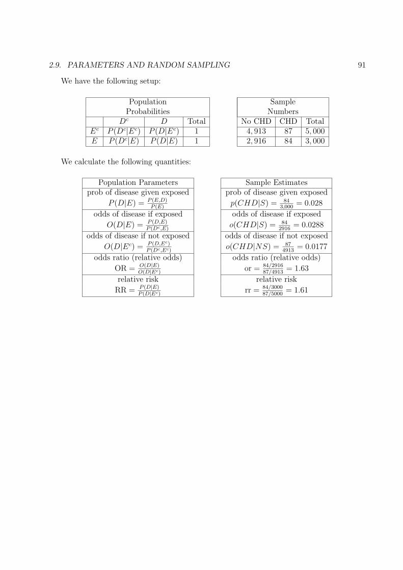
2.9. PARAMETERS AND RANDOM SAMPLING 91
We have the following setup:
Population SampleProbabilities Numbers
Dc D Total No CHD CHD TotalEc P (Dc|Ec) P (D|Ec) 1 4, 913 87 5, 000E P (Dc|E) P (D|E) 1 2, 916 84 3, 000
We calculate the following quantities:
Population Parameters Sample Estimatesprob of disease given exposed prob of disease given exposed
P (D|E) = P (E,D)P (E)
p(CHD|S) = 843,000
= 0.028
odds of disease if exposed odds of disease if exposed
O(D|E) = P (D,E)P (Dc,E)
o(CHD|S) = 842916
= 0.0288
odds of disease if not exposed odds of disease if not exposed
O(D|Ec) = P (D,Ec)P (Dc,Ec)
o(CHD|NS) = 874913
= 0.0177
odds ratio (relative odds) odds ratio (relative odds)
OR = O(D|E)O(D|Ec)
or = 84/291687/4913
= 1.63
relative risk relative risk
RR = P (D|E)P (D|Ec)
rr = 84/300087/5000
= 1.61
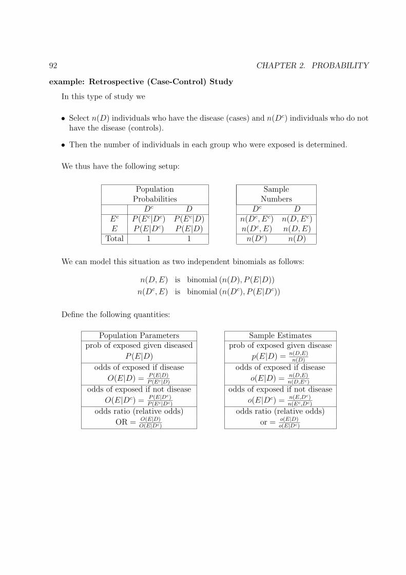
92 CHAPTER 2. PROBABILITY
example: Retrospective (Case-Control) Study
In this type of study we
• Select n(D) individuals who have the disease (cases) and n(Dc) individuals who do nothave the disease (controls).
• Then the number of individuals in each group who were exposed is determined.
We thus have the following setup:
Population SampleProbabilities Numbers
Dc D Dc DEc P (Ec|Dc) P (Ec|D) n(Dc, Ec) n(D, Ec)E P (E|Dc) P (E|D) n(Dc, E) n(D,E)
Total 1 1 n(Dc) n(D)
We can model this situation as two independent binomials as follows:
n(D,E) is binomial (n(D), P (E|D))
n(Dc, E) is binomial (n(Dc), P (E|Dc))
Define the following quantities:
Population Parameters Sample Estimatesprob of exposed given diseased prob of exposed given disease
P (E|D) p(E|D) = n(D,E)n(D)
odds of exposed if disease odds of exposed if disease
O(E|D) = P (E|D)P (Ec|D)
o(E|D) = n(D,E)n(D,Ec)
odds of exposed if not disease odds of exposed if not disease
O(E|Dc) = P (E|Dc)P (Ec|Dc)
o(E|Dc) = n(E,Dc)n(Ec,Dc)
odds ratio (relative odds) odds ratio (relative odds)
OR = O(E|D)O(E|Dc)
or = o(E|D)o(E|Dc)

2.9. PARAMETERS AND RANDOM SAMPLING 93
As an example consider the following hypothetical study in which examine individualswith coronary heart disease (CHD) (cases) and individuals without coronary heart diease(controls). We then determine which individuals were smokers and which were not. Thus Eis smoker and Ec is non smoker. This example is from Epidemiology (1996) Gordis, L. W.B. Saunders.
Population SampleProbabilities NumbersControls Cases Controls Cases
Ec P (Ec|Dc) P (Ec|D) 224 88E P (E|Dc) P (E|D) 176 112
Total 1 1 400 200
We calculate the following quantities:
Population Parameters Sample Estimatesprob of exposed given diseased prob of exposed given disease
P (E|D) p(E|D) = 112200
= 0.56odds of exposed if disease odds of exposed if disease
O(E|D) = P (E|D)P (Ec|D)
o(E|D) = 11288
= 1.27
odds of exposed if not disease odds of exposed if not disease
O(E|Dc) = P (E|Dc)P (Ec|Dc)
o(E|Dc) = 176224
= 0.79
odds ratio (relative odds) odds ratio (relative odds)
OR = O(E|D)O(E|Dc)
or = 112/88176/224
= 1.62

94 CHAPTER 2. PROBABILITY
2.10 Probability Examples
The following two examples illustrate the importance of probability in solving real problems.Each of the topics presented has been extended and generalized since their introduction.
2.10.1 Randomized Response
Suppose that a sociologist is interested in determining the prevalence of child abuse in apopulation. Obviously if individual parents are asked a question such as “have you abusedyour child” the reliability of the answer is in doubt. The sociologist would ideally like theparent to respond with an honest choice between the following two questions:
(i) Have you ever abused your children?
(ii) Have you not abused your children?
A clever method for determining prevalence in such a situation is to provide the respon-dent with a randomization device such as a deck of cards in which a proportion P of thecards are marked with the number 1 and the remainder with the number 2. The respondentselects a card at random and replaces it with the result unknown to the interviewer. Thusconfidentiality of the respondent is protected. If the card drawn is 1 the respondent answerstruthfully to question 1 whereas if the card drawn is a 2 the respondent answers truthfullyto question 2.
2.10. PROBABILITY EXAMPLES 95
It follows that the probability λ that the respondent answers yes is given by
λ = P (yes)
= P (yes|Q1)PQ1) + P (yes|Q2)PQ2)
= πP + (1− π)(1− P )
where π is the prevalence (the proportion in the population who abuse their children and Pis the proportion of 1’s in the deck of cards. We assume P 6= 1/2.
If we use this procedure on n respondents and observe x yes answers then the observedproportion x/n is a natural estimate of πP + (1− π)(1− P ) i.e.
λ =x
n= πP + (1− π)(1− P )
Since we know P we can solve for π giving us the estimate
π =λ + 1− P
2P − 1
Reference: Encyclopedia of Biostatistics.
96 CHAPTER 2. PROBABILITY
2.10.2 Screening
As another simple application of probability consider the following situation. We have afixed amount of money available to test individuals for the presence of a disease, say $1,000.The cost of testing one sample of blood is $5. We have to test a population of size 1,000 inwhich we suspect the prevalence of the disease is 3/1,000. Can we do it? If we divide thepopulation into 100 groups of size 10 then there should be 1 diseased individual in 3 of thegroups and the remaining 97 groups will be disease free. If we pool the samples from eachgroup and test each grouped sample we would need 100 + 30 = 130 tests instead of 1,000tests to screen eveyone.
The probabilistic version is as follows: A large number N of individuals are subject to ablood test which can be administered in one of two ways
(i) Each individual is to be tested separately so that N tests are required.
(ii) The samples of n individuals can be pooled or combined and tested. If this test isnegative then the one test suffices to clear all of these n individuals. If this test ispositive then each of the n individuals in that group must be tested. Thus n + 1 testsare required if the pooled samples tests positive.
Assume that individuals are independent and that each has probability p of testingpositive. Clearly we have a Bernoulli trial model and hence the probability that the combinedsample will test positive is
P (combined test positive) = 1− P (combined test negative) = 1− (1− p)n
Thus we have for any group of size n
P (1 test) = (1− p)n+1 ; P (n + 1 tests) = 1− (1− p)n
It follows that the expected number of tests if we combine samples is
(1− p)n + (n + 1)[1− (1− p)n] = n + 1− n(1− p)n
Thus if there are N/n groups we expect to run
N[1 +
1
n− (1− p)n
]
tests if we combine samples instead of the N tests if we test each individual. Given a valueof p we can choose n to minimize the total number of tests.

2.10. PROBABILITY EXAMPLES 97
As an example with N = 1, 000 and p = .01 we have the following numbers
Group Size Number of Tests2 519.93 363.03434 289.4045 249.00996 225.18657 210.79188 202.25539 197.593910 195.617911 195.570812 196.948513 199.402114 202.682815 206.608316 211.042217 215.880318 221.041819 226.46320 232.0931
Thus we should combine individuals into groups of size 10 or 11. In which case we expectto run 196 tests instead of 1,000 tests. Clearly we achieve real savings.
Reference: Feller, W. (1950 An Introduction to Probability Theory and Its Applications.John Wiley & Sons.

98 CHAPTER 2. PROBABILITY
Graph of Expected Number of Tests vs Group Size (N = 1, 000 and p = .01)
Figure 2.1:

Chapter 3
Probability Distributions
3.1 Random Variables and Distributions
3.1.1 Introduction
Most of the responses we model in statistics are numerical. It is useful to have a notation forreal valued responses. Real valued responses are called random variables. The notationis not only convenient, it is imperative when we consider statistics, defined as functions ofsample data. The probability models for these random variables are called their samplingdistributions and form the foundation of the modern theory of statistics.
Definition:
• Before the experiment is performed the possible numerical response is denoted by X,X is called a random variable.
• After the experiment is performed the observed value of X is denoted by x. We callx the realized or observed value of X.
99

100 CHAPTER 3. PROBABILITY DISTRIBUTIONS
Notation:
• The set of all possible values of a random variable X is called the sample space ofX and is denoted by X .
• The probability model of X is denoted by PX and we write
PX(B) = P (X ∈ B)
for the probability that the event X ∈ B occurs.
• The probability model for X is called the probability distribution of X.
There are two types of random variables which are of particular importance: discrete andcontinuous. These correspond to the two types of numbers introduced in the overview sectionand the two types of probability density functions introduced in the probability section.
• A random variable is discrete if its possible values (sample space) constitute a finiteor countable set e.g.
X = 0, 1 ; X = 0, 1, 2, . . . , n ; X = 0, 1, 2, . . .
Discrete random variables arise when we consider response variables which arecategorical or counts.
• A random variable is continuous or numeric if its possible values (sample space) isan interval of real numbers e.g.
X = [0,∞) ; X = (−∞,∞)
Continuous random variables arise when we consider response variables which arerecorded on interval or ratio scales.

3.1. RANDOM VARIABLES AND DISTRIBUTIONS 101
3.1.2 Discrete Random Variables
Probabilities for discrete random variables are specified by the probability density functionp(x) :
PX(B) = P (X ∈ B) =∑
x∈B
p(x)
Probability density functions for discrete random variables have the properties
• 0 ≤ p(x) ≤ 1 for all x in the sample space X• ∑
x∈X p(x) = 1
Binomial Distribution
A random variable is said to have a binomial distribution if its probability density functionis of the form:
p(x) =
(n
x
)px(1− p)n−x for x = 0, 1, 2, . . . , n
where 0 ≤ p ≤ 1.
If we define X as the number of successes in n Bernoulli trials then X is a randomvariable with a binomial distribution. The parameters are n and p where p is the probabilityof success on a given trial. The term distribution is used because the formula describes howto distribute probability over the possible values of x.
Recall that the assumptions necessary for a Bernoulli trial model to apply are:
• The result of the experiment or study consists of the result of n smaller experimentscalled trials each of which has only two possible outcomes e.g. (dead, alive), (diseased,non-diseased), (success, failure).
• The outcomes of the trials are independent.
• The probabilities of the outcomes of the trials remain the same from trial to trial(homogeneous probabilities).

102 CHAPTER 3. PROBABILITY DISTRIBUTIONS
Histograms of Binomial Distributions
Figure 3.1:
Note that as n ↑ the binomial distribution becomes more symmetric.

3.1. RANDOM VARIABLES AND DISTRIBUTIONS 103
Poisson Distribution
A random variable is said to have a Poisson distribution if its probability distribution isgiven by
p(x) =λxe−λ
x!for x = 0, 1, 2, . . .
• The parameter of the Poisson distribution is λ.
• The Poisson distribution is one of the most important distributions in the applicationsof statistics to public health problems. The reasons are:
It is ideally suited for modelling the occurence of “rare events”.
It is also particularly useful in modelling situations involving person-time.
Specific examples of situations in which the Poisson distribution applies include:
Number of deaths due to a rare disease
Spatial distribution of bacteria
Accidents
The Poisson distribution is also useful in modelling the occurence of events over time. Sup-pose that we are interested in modelling a process where:
(1) The occurrences of the event in an interval of time are independent.
(2) The probability of a single occurrence of the event in an interval of time is proportionalto the length of the interval.
(3) In any extremely short time interval, the probability of more than one occurrence ofthe event is approximately zero.
Under these assumptions:
• The distribution of the random variable X, defined as the number of occurrences ofthe event in the interval is given by the Poisson distribution.
• The parameter λ in this case is the average number of occurrences of the event in theinterval i.e.
λ = µt where µ is the rate per unit time

104 CHAPTER 3. PROBABILITY DISTRIBUTIONS
example: Suppose that the suicide rate in a large city is 2 per week. Then the probabilityof two suicides in one week is
P (2 suicides in one week) =22e−2
2!= .2707 = .271
The probability of two suicides in three weeks is
P (2 suicides in three weeks) =62e−6
2!= .0446 = .045
example: The Poisson distribution is often used as a model for the probability of automobileor other accidents for the following reasons:
(1) The population exposed is large.
(2) The number of people involved in accidents is small.
(3) The risk for each person is small.
(4) Accidents are “random”.
(5) The probability of being in two or more accidents in a short time period is approxi-mately zero.

3.1. RANDOM VARIABLES AND DISTRIBUTIONS 105
Approximations using the Poisson Distribution
Poisson probabilities can be used to approximate binomial probabilities when n is large, pis small and λ is taken to be np Thus for n = 150 and p = .02 we have the following table:
Binomial Poissonx n = 150, p = .02 λ = 150(.02) = 30 0.04830 0.049791 0.14784 0.149362 0.22478 0.224043 0.22631 0.224044 0.16974 0.168035 0.10115 0.100826 0.04989 0.050417 0.02094 0.021608 0.00764 0.008109 0.00246 0.0027010 0.00071 0.0008111 0.00018 0.0002212 0.00004 0.0000613 0.00001 0.0000114 0.00000 0.00000
Note the closeness of the approximation. The supplementary notes contain a “proof” of thepropositition that the Poisson approximates the binomial when n is large and p is small.

106 CHAPTER 3. PROBABILITY DISTRIBUTIONS
Histograms of Poisson Distributions
Figure 3.2:
Note that as n ↑ the Poisson distribution becomes more symmetric.
3.1. RANDOM VARIABLES AND DISTRIBUTIONS 107
3.1.3 Continuous or Numeric Random Variables
Probabilities for numeric or continuous random variables are given by the area under thecurve of its probability density function f(x).
P (E) =∫
Ef(x)dx
• f(x) has the properties:
f(x) ≥ 0
The total area under the curve is one
• Probabilities for numeric random variables are tabled or can be calculated using astatistical software package.
The Normal Distribution
By far the most important continuous probability distribution is the normal or Gaussian.The probability density function is given by:
p(x) =1√2πσ
exp
−(x− µ)2
2σ2
• The normal distribution is used as a basic model when theobserved data has a his-togram which is symmetric and bell-shaped.
• In addition the normal distribution provides useful approximations to other distribu-tions by the Central Limit Theorem.
• The Central Limit Theorem also implies that a variety of statistics have distributionsthat can be approximated by normal distributions.
• Most statistical methods were originally developed for the normal distribution andthen extended to other distributions.
• The parameter µ is the natural center of the distribution (since the distribution issymmetric about µ).

108 CHAPTER 3. PROBABILITY DISTRIBUTIONS
• The parameter σ2 or σ provides a measure of spread or scale.
• The special case where µ = 0 and σ2 = 1 is called the standard normal or Zdistribution

3.1. RANDOM VARIABLES AND DISTRIBUTIONS 109
The following quote indicates the importance of the normal distribution:
Thenormal
law of errorstands out in the
experience of mankindas one of the broadest
generalizations of naturalphilosophy. It serves as the
guiding instrument in researchesin the physical and social sciences and
in medicine, agriculture and engineering.It is an indispensible tool for the analysis and the
interpretation of the basic data obtained by observation and experimentation.
W. J. Youden

110 CHAPTER 3. PROBABILITY DISTRIBUTIONS
The principal characteristics of the normal distribution are
• The curve is bell-shaped.
• The possible values for x are between −∞ and +∞• The distribution is symmetric about µ
• median = mode (point of maximum height of the curve)
• area under the curve is 1.
• area under the curve over an interval I gives the probability of I
• 68% of the probability is between µ− σ and µ + σ
• 95% of the probability is between µ− 2σ and µ + 2σ
• 99.7% of the probability is between µ− 3σ and µ + 3σ
• For the standard normal distribution we have
P (Z ≥ z) = 1− P (Z ≤ z)
P (Z ≥ z0) = P (Z ≤ −z0) for z0 ≥ 0. Thus we have
P (Z ≤ 1.645) = .95
P (Z ≥ 1.645) = .05
P (Z ≤ −1.645) = .05
• Probabilities for any normal distribution can be calculated by converting to the stan-dard normal distribution (µ = 0 and σ = 1) as follows:
P (X ≤ x) = P(Z ≤ x− µ
σ
)

3.1. RANDOM VARIABLES AND DISTRIBUTIONS 111
Plot of Z Distribution
Figure 3.3:

112 CHAPTER 3. PROBABILITY DISTRIBUTIONS
Plots of Normal Distributions
Figure 3.4:

3.1. RANDOM VARIABLES AND DISTRIBUTIONS 113
Approximating Binomial Probabilities Using the Normal Distribution
If n is large we may approximate binomial probabilities using the normal distribution asfollows:
P (X ≤ x) ≈ P
Z ≤ x− np + 1
2√np(1− p)
• The 12
in the approximation is called a continuity correction since it improves theapproximation for modest values of n.
• A guideline is to use the normal approximation when
n ≥ 9
(p
1− p
)and n ≥ 9
(1− p
p
)
and use the continuity correction.
The Supplementary Notes give a brief discussion of the appropriateness of the conti-nuity correction.

114 CHAPTER 3. PROBABILITY DISTRIBUTIONS
For the Binomial distribution with n = 30 and p = .3 we find the following probabilities:
x P (X = x) P (X ≤ x)0 0.00002 0.000021 0.00029 0.000312 0.00180 0.002113 0.00720 0.009324 0.02084 0.030155 0.04644 0.076596 0.08293 0.159527 0.12185 0.281388 0.15014 0.431529 0.15729 0.5888110 0.14156 0.7303711 0.11031 0.8406812 0.07485 0.9155313 0.04442 0.9599514 0.02312 0.9830615 0.01057 0.9936316 0.00425 0.9978817 0.00150 0.99937
Thus P (Y ≤ 12) is exactly 0.91553. Using the normal approximation without the continuitycorrection yields a value of 0.88400 Using the continuity correction yields a value of 0.91841,close enough for most work. However, using STATA or other statistical packages makes iteasy to get exact probabilities.

3.1. RANDOM VARIABLES AND DISTRIBUTIONS 115
Approximating Poisson Probabilities Using the Normal Distribution
If λ ≥ 10 we can use the normal (Z) distribution to approximate the Poisson distribution asfollows:
P (X ≤ x) ≈ P
(Z ≤ x− λ√
λ
)
The following are some Poisson probabilities for λ = 10
x P (X = x) P (X ≤ x)0 0.00005 0.000051 0.00045 0.000502 0.00227 0.002773 0.00757 0.010344 0.01892 0.029255 0.03783 0.067096 0.06306 0.130147 0.09008 0.220228 0.11260 0.332829 0.12511 0.4579310 0.12511 0.5830411 0.11374 0.6967812 0.09478 0.7915613 0.07291 0.8644614 0.05208 0.9165415 0.03472 0.9512616 0.02170 0.9729617 0.01276 0.9857218 .0070911 0.9928119 .0037322 0.9965520 .0018661 0.99841
For y = 15 we find that P (≤ 15) = 0.95126 Using the normal approximation yields a valueof 0.94308 A continuity correction can again be used to improve the approximation.

116 CHAPTER 3. PROBABILITY DISTRIBUTIONS
3.1.4 Distribution Functions
For any random variable the probability that it assumes a value less than or equal to aspecified value, say x, is called its distribution function and denoted by F i.e.
F (x) = P (X ≤ x)
The distribution function F is between 0 and 1 and does not decrease as x increases. Thegraph of F is a step function for discrete random variables (the height of the step at x is theprobability of the value x) and is a differentiable function for continuous random varaibles(the derivative equals the density function).
Distribution functions are the model analogue to the empirical distribution function in-troduced in the exploratory data analysis section. They play an important role in goodnessof fit tests and in finding the distribution of functions of continuous random variables. In ad-dition, the natural estimate of the distribution function is the empirical distribution functionwhich forms the basis for the substitution method of estimation.

3.1. RANDOM VARIABLES AND DISTRIBUTIONS 117
3.1.5 Functions of Random Variables
It is often necessary to find the distribution of a function of a random variable(s).
Functions of Discrete Random Variables
In this case to find the pdf of Y = g(X) we find the probability density function directlyusing the formula
f(y) = P (Y = y) = P (x : g(x) = y)Thus if X has a binomial pdf with parameters n and p and represents the number of successesin n trials what is the pdf of Y = n−X, the number of failures? We find that
P (Y = y) = P (x : x = n− y) =
(n
n− y
)pn−y(1− p)n−(n−y) =
(n
y
)(1− p)ypn−y
i.e. binomial with parameters n and 1− p.
118 CHAPTER 3. PROBABILITY DISTRIBUTIONS
Functions of Continuous Random Variables
Here we find the distribution function of Y
P (Y ≤ y) = P (x : g(x) ≤ y)
and then differentiate to find the density function of Y .
example: Let Z be standard normal and let Y = Z2. The distribution function of Y isgiven by
F (y) = P (Y ≤ y) = P (z : −√y ≤ z ≤ √y) =
∫ √y
−√yφ(z)dz
where φ(z) is the standard normal density i.e.
φ(z) = (2π)−1/2e−z2/2
It follows that the density function of Y is equal to
dF (y)
dy=
1
2√
yφ(√
y) +1
2√
yφ(−√y)
or
f(y) =1√y(√
2π)−1/2e−y/2 =y1/2−1e−y/2
21/2√
π
which is called the chi-square distribution with one degree of freedom. That is, if Z isstandard normal then Z2 is chi-square with one degree of freedom.
3.1.6 Other Distributions
A variety of other distributions arise in statistical problems. These include the log-normal,the chi-square, the Gamma, the Beta, the t, the F , and the negative binomial. We willdiscuss these as they arise.

3.2. PARAMETERS OF DISTRIBUTIONS 119
3.2 Parameters of Distributions
3.2.1 Expected Values
In exploratory data analysis we emphasized the importance of a measure of location (center)and spread (variability) for a batch of numbers. There are analagous measures for probabilitydistributions.
Definition: The expected value, E(X), of a random variable is the weighted average ofits values, the weights being the probability assigned to the values.
• For a discrete random variable we have
E(X) =∑x
xp(x)
where p(x) is the probability density function of X.
• For continuous random variables
E(X) =∫
xxf(x)dx
Some important expected values are:
(1) The expected value of the binomial distribution is np
(2) The expected value of the Poisson distribution is λ
(3) The expected value of the normal distribution is µ

120 CHAPTER 3. PROBABILITY DISTRIBUTIONS
Using the properties of sums and integrals we have the following properties of expectedvalues
• E(c) = where c is a constant.In words: The expected value of a constant is equal to the constant.
• E(cX) = cE(X) where c is a constant.In words: The expected value of a constant times a random variable is equalto the constant times the expected value of the random variable.
• E(X + Y ) = E(X) + E(Y )In words: The expected value of the sum of two random variables is the sumof their expected values.
• If X ≥ 0 then E(X) ≥ 0In words: The expected value of a non-negative random variable is non-negative.
Note: The result that the expected value of the sum of two random variables is the sum oftheir expected values is non trivial in the sense that one must show that the distribution ofthe sum has expected value equal to the sum of the individual expected values.

3.2. PARAMETERS OF DISTRIBUTIONS 121
3.2.2 Variances
Definition: The variance of a random variable is
var (X) = E(X − µ)2 where µ = E(X)
• If we writeX = µ + (X − µ) or X = µ + error
we see that the variance of a random variable is a measure of the average size of thesquared error made when using µ to predict the value of X.
• The square root of var (X) is called the standard deviation of X and is used as abasic measure of variability for X.
(1) For the binomial var (X) = npq where q = 1− p
(2) For the Poisson var (X) = λ
(3) For the normal var (X) = σ2
Using the properties of sums and integrals we have the following properties of variances:
• var (c) = 0 where c is a constant.In words: The variance (variability) of a constant is 0.
• var (c + X) = var (X) where c is a constant.In words: The variance of a random variable is unchanged by the additionof a constant.
• var (cX) = c2var (X) where c is a constant.In words: The variance of a constant times a random variable equals theconstant squared times the variance of the random variable.
• var (X) ≥ 0In words: The variance of a random variable cannot be negative.

122 CHAPTER 3. PROBABILITY DISTRIBUTIONS
3.2.3 Quantiles
Recall that
• The median of a batch of numbers is the value which divides the batch in half.
• Similarly the upper quartile has one fourth of the numbers above it while the lowerquartile has one fourth of the numbers below it.
• There are analogs for probability distributions of random variables.
Definition: The pth quantile, Qp of X is defined by
P (X ≤ Qp) = p
where 0 < p < 1.
• Q.5 is called the median of X
• Q.25 is called the lower quartile of X
• Q.75 is called the upper quartile of X
• Q.75 −Q.25 is called the interquartile range of X

3.2. PARAMETERS OF DISTRIBUTIONS 123
3.2.4 Other Expected Values
If Y = g(X) is a function of X then Y is also a random variable and has expected valuegiven by
E[Y ] = E[g(X)] =
∑x g(x)f(x) if X is discrete∫
x g(x)f(x)dx if X is continuous
Definition: The moment generating function of X, M(t), is defined as the expectedvalue of Y = etX where t is a real number.
The moment generating function has two important theoretical properties:
(1) The rth derivative of M(t) with respect to t, evaluated at t = 0 gives the rth momentof X, E(Xr) for any integer r. This often provides an easy method to find the mean,variance, etc. of a random variable.
(2) The moment generating function is unique: that is, if two distributions have the samemoment generating function then they have the same distribution.
example: For the binomial distribution we have that
M(t) = E[etX ] =n∑
x=0
etx
(n
x
)px(1− p)n−x =
n∑
x=0
(n
x
)(pet)x(1− p)n−x = (pet + q)n
where q = 1− p. The first and second derivatives are
dM(t)dt
= npet(pet + q)n−1
d2M(t)dt2
= n(n− 1)p2e2t(pet + q)n−2 + npet(pet + q)n−1
Thus we haveE(X) = np ; E(X2) = n(n− 1)p2 + np
and hencevar (X) = n(n− 1)p2 + np− (np)2 = np(1− p)
example: For the Poisson distribution we have that
M(t) = E(etX) =∞∑
x=0
etxe−λ λx
x!== e−λ
∞∑
x=0
(λet)x
x!= eλ(et−1)

124 CHAPTER 3. PROBABILITY DISTRIBUTIONS
The first and second derivatives are
dM(t)dt
= λetM(t)d2M(t)dt2
= λ2etM(t) + λetM(t)
Thus we haveE(X) = λ ; E(X2) = λ2 + λ
and hencevar (X) = (λ2 + λ)− λ2 = λ
example: For the normal distribution we have that
M(t) = exptµ + t2σ2/2
The first two derivatives are
dM(t)dt
= (µ + tσ2)M(t)d2M(t)dt2
= (µ + tσ2)2M(t) + (σ2)M(t)
Thus we haveE(X) = µ ; E(X2) = µ2 + σ2
and hencevar (X) = (µ2 + σ2)− µ2 = σ2

3.2. PARAMETERS OF DISTRIBUTIONS 125
3.2.5 Inequalities involving Expectations
Markov’s Inequality: If Y is any non-negative random variable then
P (Y ≥ c) ≤ E(Y )
c
where c is any positive constant. To see this define a discrete random variable by the equation
Z =
c if Y ≥ c0 if Y < c
Note that Z ≤ Y so that
E(Y ) ≥ E(Z) = 0P (Z = 0) + cP (Z = c) = cP (Y ≥ c)
Tchebychev’s Inequality: If X is any random variable then
P (−δ < X − µ < δ) ≥ 1− σ2
δ2
where σ2 is the variance of X and δ is any positive number. To see this define
Y = (|X − µ|)2
Then Y is non-negative with expected value equal to σ2 and by Markov’s Inequality we havethat
P (Y ≥ δ2) ≤ σ2
δ2
and hence
1− P (Y < δ2) ≤ σ2
δ2or P (Y < δ2) ≥ 1− σ2
δ2
ButP (Y < δ2) = P (|X − µ| < δ) = P (−δ < |X − µ| < δ)
so that
P (−δ < X − µ < δ) ≥ 1− σ2
δ2

126 CHAPTER 3. PROBABILITY DISTRIBUTIONS
example: Consider n Bernoulli trials and let Sn be the number of successes. Then X = Sn/nhas
E(
Sn
n
)=
np
n= p and var
(Sn
n
)=
npq
n2=
pq
n
Thus Tchebychev’s Inequality says that
1 ≥ P(−δ <
Sn
n− p < δ
)≥ 1− pq
nδ2
In other words, if the number of trials is large, the probability that the observed frequencyof successes will be close to the true probability of success is close to 1. This is used as thejustification for the relative frequency interpretation of probability. It is also a special caseof the Weak Law of large Numbers.

Chapter 4
Joint Probability Distributions
4.1 General Case
Often we want to consider several responses simultaneously. We model these using randomvariables X1, X2, . . . and we have joint probability distributions. There are again twomajor types.
(i) Joint discrete distributions have the property that the sample space for each randomvariable is discrete and probabilities are assigned using the joint probability densityfunction defined by
0 ≤ f(x1, x2, . . . , xk) ≤ 1 ;∑x1
∑x2
· · ·∑xk
f(x1, x2, . . . , xk) = 1
(ii) Joint continuous distributions have the property that the sample space for each ran-dom variable is continuous and probabilities are assigned using the probability densityfunction which has the properties that
f(x1, x2, . . . , xk) ≥ 0∫
x1
∫
x2
· · ·∫
xk
f(x1, x2, . . . , xk)dx1dx2 · · · dxk = 1
127

128 CHAPTER 4. JOINT PROBABILITY DISTRIBUTIONS
4.1.1 Marginal Distributions
Marginal distributions are distributions of subsets of random variables which have a jointdistribution. In particular the marginal distribution of one of the components, say Xi, is saidto be the marginal distribution of Xi. Marginal distributions are obtained by “summing”or “integrating” out the other variables in the joint density. Thus if X and Y have a jointdistribution which is discrete the marginal distribution of X is given by
fX(x) =∑y
f(x, y)
If X and Y have a joint distribution which is continuous the marginal distribution of X isgiven by
fX(x) =∫
yf(x, y)dy
4.1.2 Conditional Distributions
Conditional distributions are distributions of subsets of random variables which havea joint distribution given that other components of the random variables are fixed. Theconditional distribution of Y given X = x is obtained by
fY |X(y|x) =f(y,x)
fX(x)
where f(y,x) is the joint distribution of Y and X and fX(x) is the marginal distribution ofX.
Conditional distributions are of fundamental importance in regression and predictionproblems.

4.1. GENERAL CASE 129
4.1.3 Properties of Marginal and Conditional Distributions
• The joint distribution of X1, X2, . . . , Xk can be obtained as
f(x1, x2, . . . , xk) = f1(x1)f2(xx|x1)f3(x3|x1, x2) · · · fk(xk|x1, x2, . . . , xk−1)
which is a generalization of the multiplication rule for probabilities.
• The marginal distribution of Y can be obtained via the formula
fY (y) =
∑x f(y|x)fX(x) if X,Y are discrete∫
x f(y|x)fX(x)dx if X,Y are continuous
which is is a generalization of the law of total probability.
• The conditional density of y given X = x can be obtained as
fY |X(y|x) =f(y,x)
fX(x)=
fY (y)fX|Y (x|y)
fX(x)
which is a version of Bayes Theorem.
4.1.4 Independence and Random Sampling
If X and Y have a joint distribution they are independent if
f(x,y) = fX(x)fY (y) or if fY |X(y|x) = fY (y)
In general X1, X2, . . . , Xn are independent if
f(x1, x2, . . . , xn) = fX1(x1)fX2(x2) · · · fXn(xn)
i.e. the joint distribution is the product of the marginal distributions.
Definition: We say that x1, x2, . . . , xn constitute a random sample from f if they arerealized values of independent random variables X1, X2, . . . , Xn, each of which has the sameprobability distribution f .
Random sampling from a distribution is fundamental to many applications of modernstatistics.

130 CHAPTER 4. JOINT PROBABILITY DISTRIBUTIONS
4.2 The Multinomial Distribution
The most important joint discrete distribution is the multinomial defined as
f(x1, x2, · · · , xk) = n!k∏
i=1
pxii
xi!
wherexi = 0, 1, 2, . . . , n , i = 1, 2, . . . , k ,
∑ki=1 xi = n
0 ≤ pi ≤ 1 , i = 1, 2, . . . , k ,∑k
i=1 pi = 1
The multinomial is the basis for the analysis trials where the outcomes are not binary but ofk distinct types and in the analysis of tables of data which consist of counts of the numberof times certain response patterns occur. Note that if k = 2 the multinomial reduces to thebinomial.
example: Suppose we are interested in the daily pattern of “accidents” in a manufactur-ing firm. Assuming individuals in the firm have accidents independent of others then theprobability of accidents by day has the multinomal distribution
P (x1, x2, x3, x4, x5) =n!
x1!x2!x3!x4!x5!px1
1 px22 px3
3 px44 px5
5
where pi is the probability of an accident on day i and i indexes working days. Of interestis whether or not the pi are equal. If they are not we might be interested in which seem toolarge.

4.2. THE MULTINOMIAL DISTRIBUTION 131
example: This data set consists of the cross classification of 12,763 applications for admis-sion to graduate programs at the University of California at Berkeley in 1973. The data wereclassified by gender and admission outcome. Of interest is the possibility of gender bias inthe admissions policy of the university.
Admissions OutcomeGender Admitted Not AdmittedMale 3738 4704
Female 1494 2827
In general we have that n individuals are investigated and their gender and admissionoutcome is recorded. The data are thus of the form:
Gender Admitted Not AdmittedMale n00 n01
Female n10 n11
To model this data we assume that individuals are independent and that the possible responsepatters for an individual are given by one of the following:
(male, admitted) = (0, 0)(female, admitted) = (1, 0)
(male, not admitted) = (0, 1)( female, not admitted) = (1, 1)
Denoting the corresponding probabilities by p11, p01, p10 and p00 the multinomial modelapplies and we have the probabilities of the observed responses given by
n!
n00!n01!n10!n11!pn00
00 pn0101 pn10
10 pn1111
The random variables are thus N00, N01, N10 and N11.

132 CHAPTER 4. JOINT PROBABILITY DISTRIBUTIONS
In the model above the probabilities are thus given by
Gender Admitted Not Admitted Marginal of GenderMale p00 p01 p0+
Female p10 p11 p1+
Marginal of Admission Status p+0 p+1 1
Note that p+0 gives the probability of admission and that p0+ gives the probability of be-ing male. It is clear (why?) that the marginal distribution of admission is binomial withparameters n and p = p+0.
The probability that N00 = n00 and N01 = n01 given that N00 + N01 = n0+ gives theprobability of admission given male and is
P (N00 = n00, N01 = n01|N00 + N01 = n0+)
This conditional probability is given by:
P (N00 = n00, N01 = n0+ − n00)
P (N00 + N01 = n0+)=
n!(n0+−n00)!n00!(n−n0+)!
n!n0+!(n−n0+)!
pn0000 p
n0+−n00
01 (1− p0+)n−n0+
pn0+
0+ (1− p0+)n−n0+
=n0+!
n00!(n0+ − n00)!
(p00
p0+
)n00(
p01
p0+
)n0+−n00
=
(n0+
n00
)pn00∗ (1− p∗)n0+−n00
which is a binomial distribution with parameters n0+, the number male and
p∗ =p00
p0+
Note that the odds of admission given male arep∗
1− p∗=
p00
p01
Similarly the probability of admission given female is binomial with parameters n1+, thenumber of females and P∗ where
P∗ =p10
p1+
Note that the odds in this case are given by
P∗1− P∗
=p10
p11
4.2. THE MULTINOMIAL DISTRIBUTION 133
Thus the odds ratio of admission (female to male) is given by
p10/p11
p00/p01
=p01p10
p00p11
If the odds ratio is one gender and admission are independent. (Why?) It follows that theodds ratio is a natural measure of association for categorical data.
In the example the odds of admission for males is estimated by
odds of admission for males =3738/8442
4704/8442=
3738
4704= 0.79
while the odds for admission given female is
odds of admission given female =1494/4321
2827/4321=
1494
2827= 0.53
Thus the odds of admission are lower for females. The odds ratio is estimated by
odds ratio of admission (females to males) =1494/2827
3738/4704=
1494× 4704
2827× 3738= 0.67
Is this odds ratio different enough from 1 to claim that females are discriminated againstin the admissions policy? More later!!!

134 CHAPTER 4. JOINT PROBABILITY DISTRIBUTIONS
4.3 The Multivariate Normal Distribution
The most important joint continuous distribution is the multivariate normal distribution.The density function of Y is given by
f(x) = (2π)−k2 [det(V)]−
12 exp
−1
2(x− µ)TV−1(x− µ)
where we assume that V is a non-singular, symmetric, positive definite matrix of rank k.The two parameters of this distribution are µ and V.
• It can be shown that the marginal distribution of any Xi is normal with parametersµi and vii where
µ =
µ1
µ2...
µk
, V =
v11 v12 · · · v1k
v12 v22 · · · v2k...
......
...v1k v2k · · · vkk
• It can also be shown that the distribution of linear combinations of multivariate normalrandom variables are also multivariate normal. More precisely let W = a+BY wherea is p × 1 and B is a p × k matrix with p ≤ k. Then the joint distribution of W ismultivariate normal with parameters
µW = a + BµY and VW = BVY BT
where BT is the transpose of B.

4.3. THE MULTIVARIATE NORMAL DISTRIBUTION 135
• It can also be shown that the conditional distribution of any subset of X given anyother subset is multivariate normal more precisely: let
X =
[X1
X2
]; µ =
[µ1
µ2
], V =
[V11 V12
VT12 V22
]
where AT denotes the transpose of A. Then the conditional distribution of X2 givenX1 = x1 is also multivariate normal with
µ∗ = µ2 + VT12V
−111 (x1 − µ1) ; V∗ = V22 −VT
12V−111 V12
• It follows that if X1 and X2 have a multivariate normal distribution then they areindependent if and only if
V12 = 0
The multivariate normal distribution forms the basis for regression analysis, analysisof variance and a variety of other statistical methods including factor analysis and latentvariable analysis.

136 CHAPTER 4. JOINT PROBABILITY DISTRIBUTIONS
4.4 Parameters of Joint Distributions
4.4.1 Means, Variances, Covariances and Correlation
The collection of expected values of the marginal distributions of Y is called the expectedvalue of Y and is written as
E(Y) = µ =
E(Y1)E(Y2)
...E(Yk)
=
µ1
µ2...
µk
The covariance between X and Y , where X and Y have a joint distribution is defined by
cov (X,Y ) = E(X − µX)(Y − µY )
The correlation between X and Y is defined as
ρ(X,Y ) =cov (X, Y )√
var (X)var (Y )
and is simply a standardized covariance. Correlations have the property that
−1 ≤ ρ(X, Y ) ≤ 1

4.4. PARAMETERS OF JOINT DISTRIBUTIONS 137
Using the properties of expected values we see that covariances have the following prop-erties
• cov (X,Y ) = cov (Y,X)
• cov (X,X) = var (X)
• cov (X + a, Y + b) = cov (X, Y )
• cov (aX, bY ) = abcov (X, Y )
• cov (aX + bY, cW + dZ) = ac cov (X, W ) + ad cov (X, Z) + bc cov (Y, W ) + bd cov (Y, Z)
We define the variance covariance matrix of Y as
VY =
var (Y1) cov (Y1, Y2) · · · cov (Y1, Yk)cov (Y1, Y1) var (Y2) · · · cov (Y2, Yk)
......
. . ....
cov (Yk, Y1) cov (Yk, Y2) · · · var (Yk, Yk)
Note that for the multivariate normal distribution with parameters µ and V we havethat
E(Y) = µ and VY = V
Thus the two parameters in the multivariate normal are respectively the mean vector andthe variance covariance matrix.

138 CHAPTER 4. JOINT PROBABILITY DISTRIBUTIONS
4.4.2 Joint Moment Generating Functions
The joint moment generating function of X1, X2, . . . , Xk is defined as
MX(t) = E(e∑k
i=1tiXi)
• Partial derivatives with respect to ti evaluated at t1 = t2 = · · · = tk = 0 give themoments of Xi and mixed partial derivatives (e.g. with respect to ti and tj give thecovariances, etc.)
• Joint moment generating functions are unique (if two distributions have the samemoment generating function then the two distributions are the same).
• The joint moment generating function for the multivariate normal distribution is givenby
MX(t) = expµT t +
1
2tTVt
= exp
k∑
i=1
tiµi +1
2
k∑
i=1
k∑
j=1
titjvij
• If random variables are independent then their joint moment generating function isequal to the product of the individual moment generating functions.

4.5. FUNCTIONS OF JOINTLY DISTRIBUTED RANDOM VARIABLES 139
4.5 Functions of Jointly Distributed Random Variables
If Y = g(X) is any function of random variables X we can find its distribution exacly as inthe one variable case i.e.
fY (y) =∑
x:g(x)=y f(x1, x2, . . . , xk) if X is discrete
fY (y) = dFY (y)dy
if X is continuous
whereFY (y) =
∫
x:g(x)≤yf(x1, x2, . . . , xk)dx1dx2 · · · dxk
Thus we can find the distribution of the sum, the difference, a linear combination, aratio, a product, etc. We shall not derive all of the results we use in later sections but weshall record a few of the most important results here
• If X has a multivariate normal distribution with mean µ and variance covariancematrix V then the distribution of
Y = a + bTX = a +k∑
i=1
biXi
is normal with
E(Y ) = a + bT µ = a +k∑
i=1
biE(Xi) and var (Y ) = bTVb =k∑
i=1
k∑
j=1
bibjcov (Xi, Xj)
140 CHAPTER 4. JOINT PROBABILITY DISTRIBUTIONS
• If Z1, Z2, . . . , Zr are independent each N(0, 1) then the distribution of
Z21 + Z2
2 + · · ·+ Z2r
is chi-square with r degrees of freedom.
• If Z is N(0, 1) and W is chi-square with r degrees of freedom and Z and W areindependent then
T =Z√W/r
has a Student’s t distribution with r degrees of freedom.
• If Z1 and Z2 are each N(0, 1) and independent then the distribution of the ratio
C =Z1
Z2
is Cauchy with parameters 0 and 1

4.5. FUNCTIONS OF JOINTLY DISTRIBUTED RANDOM VARIABLES 141
4.5.1 Linear Combinations of Random Variables
If X1, X2, . . . , Xn have a joint distribution with parameters µ1, µ2, . . . , µn and variances andcovariances given by
cov (Xi, Xj) = vij
then the expected value of∑n
i=1 aiXi is given by
E(n∑
i=1
aiXi) =n∑
i=1
aiE(µi) =n∑
i=1
aiµi
and the variance of∑n
i=1 aiXi is given by
var
(n∑
i=1
aiXi
)=
n∑
i=1
n∑
j=1
aiajcov (Xi, Xj) =n∑
i=1
n∑
j=1
aiajvij
If we write
µ =
µ1
µ2...
µn
; V =
v11 v12 · · · v1n
v21 v22 · · · v2n...
.... . .
...vn1 vn2 · · · vnn
we see that the above results may be written as
E(aTX) = aT µ ; var (aTX) = aTVa
142 CHAPTER 4. JOINT PROBABILITY DISTRIBUTIONS
As special cases we have
• var (X + Y ) = var (X) + var (Y ) + 2 cov (X, Y )
• var (X − Y ) = var (X) + var (Y )− 2 cov (X, Y )
• Thus if X and Y are uncorrelated with the same variance σ2 we hav
– var (X + Y ) = 2σ2
– var (X − Y ) = 2σ2
• More generally if X1, X2, . . . , Xn are uncorrelated then
var
(n∑
i=1
aiXi
)=
n∑
i=1
a2i var (Xi)
– In particular if we take each ai = 1n
we have
var (X) =σ2
n

4.6. APPROXIMATE MEANS AND VARIANCES 143
4.6 Approximate Means and Variances
In some problems we cannot find the expected value or variance or distribution of Y = g(X)exactly. It is useful to have approximations for the means and variances in such cases. Ifthe function g is reasonably linear in a neignorhood of µX , the expected value of X then wecan write
Y = g(X) ≈ g(µ) + g(1)(µX)(X − µX)
by Taylor’s Theorem. Hence we have
E(Y ) ≈ g(µX)var (Y ) ≈ [g(1)(µX)]2σ2
X
We can get an improved approximation to the expected value of Y by writing
Y = g(X) ≈ g(µ) + g(1)(µX)(X − µX) +1
2g(2)(µX)(X − µX)2
Thus
E(Y ) ≈ g(µX) +1
2g(2)(µX)σ2
X

144 CHAPTER 4. JOINT PROBABILITY DISTRIBUTIONS
If Z = g(X,Y ) is a function of two random variables then we can write
Z = g(X,Y ) ≈ g(µ) +∂g(µ)
∂x(X − µX) +
∂g(µ)
∂y(Y − µY )
where µ denotes the point (µX , µY ) and
∂g(µ)
∂x=
∂g(x, y)
∂x
∣∣∣∣∣x=µX ,y=µY
Thus we have that
E(Z) ≈ g(µ)
var (Z) ≈[
∂g(µ)∂x
]2σ2
X +[
∂g(µ)∂y
]2σ2
y + 2[
∂g(µ)∂x
] [∂g(µ)
∂y
]cov (X, Y )
As in the single variable case we can obtain an improved approximation for the expectedvalue by using Taylor’s Theorem with second order terms e.g.
E(Z) ≈ g(µ) +1
2
[∂2g(µ)
∂x2
]σ2
X +1
2
[∂2g(µ)
∂y2
]σ2
Y +
[∂2g(µ)
∂x∂y
]cov (X, Y )
• Note 1: The improved approximation is needed for the expected value because ingeneral E[g(X)] 6= g(µ) i.e. E(X2) 6= µ2
• Note 2: Some care is needed when working with discrete variables and certain functions.Thus if X is binomial with parameters n and p the expected value of log(X) is notdefined so that no approximation can be correct.

4.7. SAMPLING DISTRIBUTIONS OF STATISTICS 145
4.7 Sampling Distributions of Statistics
Definition: A statistic is a numerical quantity calculated from a set of data. Typically astatistic is designed to provide information about some parameter of the population.
• If x1, x2, . . . , xn is the data some statistics are
– x, the sample mean
– the median
– the upper quartile
– s2, the sample variance
– the range
• Since the data are realized values of random variables a statistic is also realized valueof a random variable.
• The probability distribution of this random variable is called the sampling distribu-tion of the statistic.

146 CHAPTER 4. JOINT PROBABILITY DISTRIBUTIONS
In most contemporary applications of statistics the sampling distribution of the statistic isused to assess the performance of a statistic used for inference about population parameters.The following is a schematic diagram of the concept of a sampling distribution of a statistics.experiment.
Figure 4.1:

4.7. SAMPLING DISTRIBUTIONS OF STATISTICS 147
Illustration of Sampling DistributionsSampling Distribution of Sample Mean, Sample Size 25
Figure 4.2:

148 CHAPTER 4. JOINT PROBABILITY DISTRIBUTIONS
Illustration of Sampling DistributionsSampling Distribution of (n− 1)s2/σ2, Sample Size n = 10
Figure 4.3:

4.7. SAMPLING DISTRIBUTIONS OF STATISTICS 149
Illustration of Sampling DistributionsSampling Distribution of t =
√n(x− µ)/s, Sample Size n = 10
Figure 4.4:

150 CHAPTER 4. JOINT PROBABILITY DISTRIBUTIONS
example: Given a sample of data suppose we calculate the sample mean x and the samplemedian q.5. Which of these is a better measure of the center of the population?
• If we assume that the data represent a random sample from a probability distributionwhich is N(µ, σ2) then it is known that:
the sampling distribution of X is N(µ, σ2
n)
the sampling distribution of the sample median is approximately N(µ, (π2)σ2
n).
• Thus the sample mean will, on average, be closer to the population mean than will thesample median. Thus the sample mean is preferred as as estimate of the populationmean.
• If the underlying population is not N(µ, σ2) then the above result does not hold andthe sample median may be the preferred estimate.
• It follows that the role of assumptions about the underlying probability model is crucialin the development and assesment of statistical procedures.

4.8. METHODS OF OBTAINING SAMPLING DISTIBUTIONS OR APPROXIMATIONS151
4.8 Methods of Obtaining Sampling Distibutions or
Approximations
There are three methods used to obtain information on sampling distributions:
• Exact sampling distributions. Statisticians have, over the last 100 years, developed thesampling distributions for a variety of useful statistics for specific parametric models.For the most part these statistics are simple functions of the sample data such as thesample mean, the sample variance, etc.
• Asymptotic (approximate) distributions. When exact sampling distributions are nottractable we may find the distribution of the statistic for large sample sizes. These arecalled asymptotic methods and are suprisingly useful.
• Computer intensive methods. These are based on resampling from the empirical distri-bution of the data and have been shown to have useful properties. The most importantof these methods is called the bootstrap.
4.8.1 Exact Sampling Distributions
Here we find the exact sampling distribution of the statistic using the methods previouslydiscussed. The most famous example of this method is the result that if we have a randomsample for a normal distribution then the distribution of the sample mean is also normal.Other examples include the distribution of the sample variance from a normal sample, the tdistribution and the F distribution.

152 CHAPTER 4. JOINT PROBABILITY DISTRIBUTIONS
4.8.2 Asymptotic Distributions
4.8.3 Central Limit Theorem
If we cannot find the exact sampling distribution of a statistic we may be able to find itsmean and variance. If the sampling distribution were approximately normal then we wouldbe able to make approximate statements using just the mean and variance. In the discussionof the Binomial and Poisson distributions we noted that for large n the distributions couldbe approximated by the normal distribution.
• In fact, the sampling distribution of X for almost any population distribution becomesmore and more similar to the normal distribution regardless of the shape of the originaldistribution as n increases.
More precisely:
Central Limit Theorem If X1, X2, . . . , Xn are independent each with the same distributionhaving expected value µ and variance σ2 then the sampling disribution of X is approximatelyN(µ, σ2
n) i.e.
P
X − µ
σ√n
≤ z
∼ P (Z ≤ z)
where P (Z ≤ z) is the area under the normal curve up to z.
The Central Limit Theorem has been extended and refined over the last 75 years.
• Many statistics have distributions whose sampling distributions are approximately nor-mal.
• This explains the great use of the normal distribution in statistics.
• In particular, whenever a measurement can be thought of as a sum of individual com-ponents we may expect it to be approximately normal.

4.8. METHODS OF OBTAINING SAMPLING DISTIBUTIONS OR APPROXIMATIONS153
4.8.4 Central Limit Theorem Example
We now illustrate the Central Limit Theorem and some other results on sampling distri-butions. The data set consists of a population of 1826 children whose blood lead values(milligarms per deciliter) were recorded at the Johns Hopkins Hospital. The data are cour-tesy of Dr. Janet Serwint. Lead in children is a serious public health problem, lead levelsexceeding 15 milligrams per deciliter are considered to have implications for learning disabil-ities, are implicated in violent behavior and are the concern of major governmental effortsaimed at reducing exposure.
The distribution in real populations is often assumed to follow a log-normal distributioni.e. the natural logarithm of blood lead values is normally distributed.
Note the asymmetry of the distribution of blood lead values. Note that the log trans-formation results in a decided improvement in symmetry, indicating that the log-normalassumption is probably appropriate.
We select random samples from the population of blood lead readings and log bloodlead readings. We select 100 random samples of size 10, 25 and 100 respectively. As thehistograms indicate the distribution of the sample means of the blood lead values do indeedappear normal even though the distribution of blood lead values is highly skewed.

154 CHAPTER 4. JOINT PROBABILITY DISTRIBUTIONS
Histograms of Blood Lead and Log Blood Lead Values
Figure 4.5:

4.8. METHODS OF OBTAINING SAMPLING DISTIBUTIONS OR APPROXIMATIONS155
Histograms of Sample Means of Blood Lead Values
Figure 4.6:

156 CHAPTER 4. JOINT PROBABILITY DISTRIBUTIONS
Histograms of Sample Means of Log Blood Lead Values
Figure 4.7:

4.8. METHODS OF OBTAINING SAMPLING DISTIBUTIONS OR APPROXIMATIONS157
The summary statistics for blood lead values and the samples are as follows
> summary(blpb)
Min. 1st Qu. Median Mean 3rd Qu. Max.
0 5 8 9.773 12 128
> var(blpb)
71.79325
Sample Size Mean Variance10 9.93 9.5325 9.75 2.91100 9.87 .72
The summary statistics for log blood lead values and the samples are as follows
summary(logblpb)
Min. 1st Qu. Median Mean 3rd Qu. Max.
-1.386 1.658 2.11 2.084 2.506 4.854
> var(logblpb)
[1] 0.4268104
Sample Size Mean Variance10 2.07 .03725 2.08 .017100 2.08 .004
158 CHAPTER 4. JOINT PROBABILITY DISTRIBUTIONS
4.8.5 Law of Large Numbers
Under most weak conditions, the average of a sample is “close” to the population average ifthe sample size is large. More precisely:
Law of Large Numbers: If we have a random sample X1, X2, . . . , Xn from a distributionwith expected value µ and variance σ2 then
P (X ≈ µ) ≈ 1
for n sufficiently large. The approximation becomes closer the larger the value of n.
We write Xp−→ µ and say that X converges in probability to µ. If g is a continuous
function then if X converges in probability to µ then g(X) converges in probability to g(µ).
Some idea of the value of n needed can be obtained from Chebychev’s inequality whichstates that
P (−k ≤ X − µ ≤ k) ≥ 1− σ2
n k2
where k is any constant.

4.8. METHODS OF OBTAINING SAMPLING DISTIBUTIONS OR APPROXIMATIONS159
Law of Large Numbers Examples
Figure 4.8:

160 CHAPTER 4. JOINT PROBABILITY DISTRIBUTIONS
4.8.6 The Delta Method - Univariate
For statistics Sn which are normal or approximately normal the delta method can be usedto find the approximate distribution of g(Sn), a function of Sn.
The technique is based on approximating g by a linear function as in obtaining approxi-mations to expected values and variances of functions i.e.
g(Sn) ≈ g(µ) + g(1)(µ)(Sn − µ)
where Sn converges in probability to µ and g(1)(µ) is the derivative of g evaluated at µ.
Thus we have thatg(Sn)− g(µ) ≈ g(1)(µ)(Sn − µ)
If√
n(Sn−µ) has an exact or approximate normal distribution with mean 0 and varianceσ2 then √
n[g(Sn)− g(µ)]
has an approximate normal distribution with mean 0 and variance
[g(1)(µ)]2σ2
It follows that we may make approximate calculations by treating g(Sn) as if were normalwith mean g(µ) and variance [g(1)(µ)]2σ2/n i.e.
P (g(Sn) ≤ s) = P
g(Sn)− g(µ)√
[g(1)(µ)]2σ2/n
≤ x− g(µ)√[g(1)(µ)]
2σ2/n
= P
Z ≤ x− g(µ)√
[g(1)(µ)]2σ2/n
where Z is N (0, 1). in addition if g(1)(µ) is continous then we can replace µ by Sn in theformula for the variance.

4.8. METHODS OF OBTAINING SAMPLING DISTIBUTIONS OR APPROXIMATIONS161
example: Let X be binomial with parameters n and p and let Sn = X/n. Then we knowby the Central Limit Theorem that the approximate distribution of
√n(Sn − p)
is N (0, pq). If we define
g(x) = ln(
x
1− x
)= ln(x)− ln(1− x)
then
g(1)(x) =1
x+
1
(1− x)=
(1− x) + x
x(1− x)=
1
x(1− x)
Thus
g(1)(µ) =1
pq
and hence √n
[ln
(Sn
1− Sn
)− ln
(p
1− p
)]
is approximately normal with mean 0 and variance
pg
(pq)2=
1
p+
1
q
Since g(1)(µ) is continuous we may treat ln(Sn) as if it where normal with
mean ln
(p
1− p
)and variance
1
n
[1
Sn
+1
1− Sn
]=
1
X+
1
n−X
Thus the distribution of the sample log odds in a binomial may be approximated by a normaldistribution with mean equal to the population log odds and variance equal to the sum ofthe reciprocals of the number of successes and the number of failures.

162 CHAPTER 4. JOINT PROBABILITY DISTRIBUTIONS
4.8.7 The Delta Method - Multivariate
More generally, if we have a collection of statistics S1, S2, . . . , Sk then we say that theyare approximately multivariate normally distributed with mean µ and variance covariancematrix V if √
n aT (Sn − µ)
has an approximate normal distribution with mean 0 and variance aTVa for any a.
In this case the distribution of g(Sn) is also approximately normal i.e.
√n [g(Sn)− g(µ)]
is approximately normal with mean 0 and variance σ2g = ∇(µ)TV∇(µ) where
∇(µ) =
∂g(µ)
∂µ1∂g(µ)
∂µ2
...∂g(µ)
∂µk2
Thus we may make approximate calculations by treating g(Sn) as if were normal with withmean g(µ) and variance σ2
g i.e.
P (g(Sn) ≤ s) = P
g(Sn)− g(µ)√
σ2g/n
≤ s− g(µ)√σ2
g/n
= P
Z ≤ x− g(µ)√
σ2g/n
where N (0, 1). In addition if each partial derivative is continuous we may replace µ by Sn
in the formula for the variance.

4.8. METHODS OF OBTAINING SAMPLING DISTIBUTIONS OR APPROXIMATIONS163
example: Let X1 be binomial n and p1 and let X2 be binomial n and p2 and be independent.Then then the joint distribution of
Sn =
[S1n
S2n
]=
[X1/nX2/n
]
is such that √n(Sn − p)
is approximately multivariate normal with mean 0 and variance covariance matrix V where
V =
[p1q1 00 p2q2
]
Thus if
g(p) = ln
(p2
1− p2
)− ln
(p1
1− p1
)= ln(p2)− ln(1− p2)− ln(p1) + ln(1− p1)
we have that∂g(p)∂p1
= − 1p1− 1
1−p1= − 1
p1q1∂g(p)∂p2
= 1p2
+ 11−p2
= 1p2q2
It follows that
σ2g =
[− 1
p1q1
1p2q2
] [p1q1 00 p2q2
] [ − 1p1q11
p2q2
]=
1
p1q1
+1
p2q2
Since the partial derivatives are continuous we may treat the sample log odds ratio as if itwhere normal with mean equal to the population log odds ratio
ln
(p2/(1− p2)
p1/(1− p1)
)
and variance1
X1
+1
n−X1
+1
X2
+1
n−X2
164 CHAPTER 4. JOINT PROBABILITY DISTRIBUTIONS
If we write the sample data as
sample 1 X1 = a n−X1 = bsample 2 X2 = c n−X2 = d
then the above formula reads as1
a+
1
b+
1
c+
1
d
a very widely used formula in epidemiology.
Technical Notes
(1) Only a minor modification is needed to show that the result is true when the samplesize in the two binomials is different provided that the ratio of the sample sizes doesnot tend to 0.
(2) The log odds ratio is much nearly normally distributed than the odds ratio.
We generate 1000 samples of size 20 from each of two binomial populations one with param-eter .3 and the other with parameter .5. It follows that the population odds ratio and thepopulation log odds ratio are given by
odds ratio =.5/.5
.3/.7=
7
3= 2.333 ; log odds ratio = .8473
The asymptotic variance for the log odds ratio is given by the formula
(1/6) + (1/14) + (1/10) + (1/10) = .4381
which leads to an asymptotic standard deviation of .6618.
The mean of the 1000 random samples is .9127 with variance .5244 and standard deviation.7241.

4.8. METHODS OF OBTAINING SAMPLING DISTIBUTIONS OR APPROXIMATIONS165
Graphs of the Simulated Distributions
Figure 4.9:

166 CHAPTER 4. JOINT PROBABILITY DISTRIBUTIONS
4.8.8 Computer Intensive Methods
• The determination of the sampling distribution of statistics which are complicatedfunctions of the observations can be approximated using the Delta Method.
• With the advent of fast modern computing techniques other methods of obtainingsampling distributions have been developed. One of these, called the bootstrap is ofgreat importance in estimation and in interval estimation.
The Bootstrap Method
Given data x1, x2, . . . , xn, a random sample from p(x; θ) we estimate θ by the statistic θ. Ofinterest is the standard error of θ. We may not be able to obtain the standard error if θis a complicated function of the data, nor do we want an asymptotic result which may besuspect if used for small samples.
The bootstrap method, introduced in 1979 by Bradley Efron, is a computer intensivemethod for obtaining the standard error of θ which has been shown to valid in most situations.The bootstrap method for estimating the standard error of θ is as follows:
(1) Draw a random sample of size n with replacement from the observed data x1, x2, . . . , xn
and compute θ.
(2) Repeat step 1 a large number, B, of times obtaining B separate estimates of θ denotedby
θ1, θ2, . . . , θB
(3) Calculate the mean of the estimates in step 2 i.e.
θ =
∑Bi=1 θi
B
(4) The bootstrap estimate of the standard error of θ is given by
σBS(θ) =
√√√√∑B
i=1(θi − θ)2
B − 1

4.8. METHODS OF OBTAINING SAMPLING DISTIBUTIONS OR APPROXIMATIONS167
The bootstrap is computationally intensive but is easy to use except in very complexproblems. Efron suggests about 250 samples be drawn (i.e. B=250) in order to obtainreliable estimates of the standard error. To obtain percentiles of the bootstrap distributionit is suggested that 500 to 1000 bootstrap samples be taken. The following is a schematic ofthe bootstrap procedure.
Figure 4.10:

168 CHAPTER 4. JOINT PROBABILITY DISTRIBUTIONS
It is interesting to note that the current citation index for statistics lists about 600 papersinvolving use of the bootstrap!
References:
1. A Leisurely Look at the Bootstrap, the Jackknife and Cross-Validation (1983) B. Efronand G. Gong; The American Statistician, February 1983, Vol. 37, No. 1
2. Bootstrapping (1993) C. Mooney and R. Duval; Sage Publications. This is a veryreadable introduction designed for applications in the Social Sciences.
3. The STATA Manual has an excellent section on the bootstrap and a bootstrap com-mand is available.
The Jackknife Method
The jackknife is another procedure for obtaining estimates and standard errors in situationswhere
• The exact sampling distribution of the estimate is not known.
• We want an estimate of the standard error of the estimate which is robust againstmodel failure and the assumption of large sample sizes.
The jackknife is computer intensive but relatively easy to implement.

4.8. METHODS OF OBTAINING SAMPLING DISTIBUTIONS OR APPROXIMATIONS169
Assume that we have n observations x1, x2, . . . , xn which are assumed to be a randomsample from a distribution p. Assume the parameter of interest is θ and that the estimateis θ
The jackknife procedure is as follows:
1. Let θ(i) denote the estimate of θ determined by eliminating the ith observation.
2. The jackknife estimate of θ is defined by
θ(JK) =1
n
n∑
i=1
θ(i)
i.e. the average of the θ(i).
3. The jackknife estimate of the standard error of θ is given by
σJK =
[(n− 1)
n
n∑
i=1
(θ(i) − θ(JK))2
]1/2

170 CHAPTER 4. JOINT PROBABILITY DISTRIBUTIONS
4.8.9 Bootstrap Example
In ancient Greece a rectangle was called a “Golden Rectangle” if the length to width ratiowas
2√5 + 1
= 0.618034
This ratio was a design feature of their architecture. The following data set gives the breadthto length ratio of beaded rectangles used by the Shoshani Indians in the decoration of leathergoods. Were they also using the Golden Rectangle?
.693 .672 .668 .553
.748 .615 .611 .570
.654 .606 .606 .844
.670 .690 .609 .576
.662 .628 .601 .933
We now use the bootstrap method for the sample mean and the sample median.

4.8. METHODS OF OBTAINING SAMPLING DISTIBUTIONS OR APPROXIMATIONS171
. infile ratio using "c:\courses\b651201\datasets\shoshani.raw
(20 observations read)
. stem ratio
Stem-and-leaf plot for ratio
ratio rounded to nearest multiple of .001
plot in units of .001
5** | 53,70,76
6** | 01,06,06,09,11,15,28
6** | 54,62,68,70,72,90,93
7** | 48
7** |
8** | 44
8** |
9** | 33
. summarize ratio
Variable | Obs Mean Std. Dev. Min Max
---------+-----------------------------------------------------
ratio | 20 .66045 .0924608 .553 .933
172 CHAPTER 4. JOINT PROBABILITY DISTRIBUTIONS
. bs "summarize ratio" "r(mean)", reps(1000) saving(mean)
command: summarize ratio
statistic: r(mean)
(obs=20)
Bootstrap statistics
Variable | Reps Observed Bias Std. Err. [95% Conf. Interval]
---------+-------------------------------------------------------------------
bs1 | 1000 .66045 .0017173 .0197265 .6217399 .6991601 (N)
| .626775 .70365 (P)
| .6264 .7021 (BC)
-----------------------------------------------------------------------------
N = normal, P = percentile, BC = bias-corrected
. use mean, clear
(bs: summarize ratio)
. kdensity bs1
. kdensity bs1,saving(g1,replace)
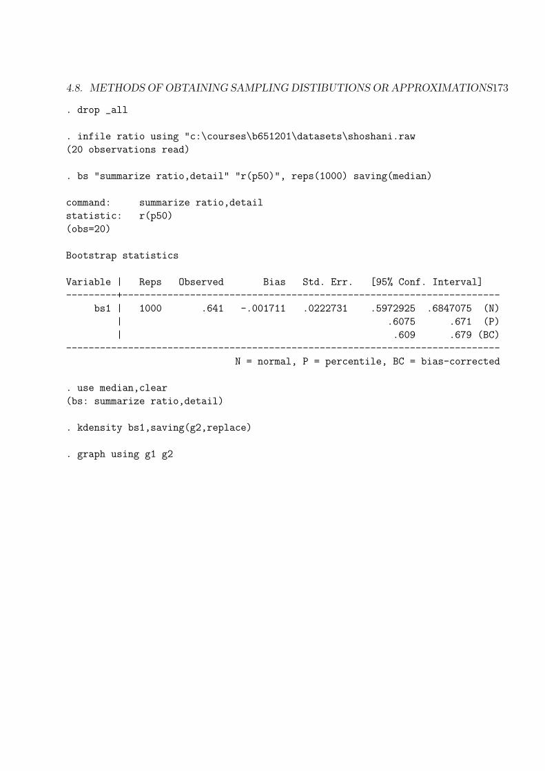
4.8. METHODS OF OBTAINING SAMPLING DISTIBUTIONS OR APPROXIMATIONS173
. drop _all
. infile ratio using "c:\courses\b651201\datasets\shoshani.raw
(20 observations read)
. bs "summarize ratio,detail" "r(p50)", reps(1000) saving(median)
command: summarize ratio,detail
statistic: r(p50)
(obs=20)
Bootstrap statistics
Variable | Reps Observed Bias Std. Err. [95% Conf. Interval]
---------+-------------------------------------------------------------------
bs1 | 1000 .641 -.001711 .0222731 .5972925 .6847075 (N)
| .6075 .671 (P)
| .609 .679 (BC)
-----------------------------------------------------------------------------
N = normal, P = percentile, BC = bias-corrected
. use median,clear
(bs: summarize ratio,detail)
. kdensity bs1,saving(g2,replace)
. graph using g1 g2

174 CHAPTER 4. JOINT PROBABILITY DISTRIBUTIONS
The bootstrap distributions of the sample mean and the sample median are given below:
Figure 4.11: