1

Part V. Time and Frequency Characterization of Signals and Systems

Topics to be covered

a. Introduction b. The magnitude phase representation of the Fourier transform

c. The magnitude phase representation of the frequency response of LTI systems

d. First-order and second order continuous and discrete time systems e. Time and frequency domain analysis

V.1. Introduction In system design, there are both time domain and frequency domain considerations. It is important to relate the time-domain and frequency domain characteristics and trade-offs.

V.2. The magnitude phase representation of the Fourier transform The magnitude-phase representation of the continuous-time Fourier transform )( jwX is

)()()( jwXjejwXjwX ∠=

Similarly the magnitude-phase representation of the discrete-time Fourier transform )( jweX is )()()(

jweXjjwjw eeXeX ∠= Remarks: The same essential points apply both to continuous time system and to the discrete time case.

)( jwX decomposes the signal )(tx into a sum of complex exponentials at different frequencies. 2)( jwX may be interpreted as the energy-density spectrum of )(tx .

The magnitude )( jwX describes the basic frequency content of a signal. The phase angle )( jwX∠ , on the other hand, does not affect the amplitudes of the individual frequency components. It provides us with information concerning the relative phase of these exponents

2

Remarks: in some instances, phase distortion may be important (images), whereas in others it is not (audio signal)

V.3. The magnitude phase representation of the frequency response of LTI systems

H(jw)X(jw) Y(jw)

The transform of the output of an LTI system )( jwY is related to the transform of the input

)( jwX by the equation: )()()( jwXjwHjwY =

Similar for discrete time system:

)()()( jwjwjw eXeHeY =

In continuous time:

Magnitude: )()()( jwXjwHjwY = and phase: )()()( jwXjwHjwY ∠+∠=∠

)( jwH∠ is typically referred to as the phase shift of the system. V.3.1) Linear and Nonlinear phase Consider the continuous time LTI system with frequency response:

0)( jwtejwH −= The system has the magnitude of 1)( 0 == − jwtejwH and linear phase 0)( wtjwH −=∠ The system with this frequency response characteristic produce an output that is simply a time shift of the input )()( 0ttxty −= In discrete-time case, the effect of linear phase is similar to that in the continuous time case

][][)( 00 nnxnyeeH jwnjw −=⇒= −

Remarks: 1) Linear phase shifts lead to simple changes in signal. The phase slope yields the size of the time shift. 2) Nonlinear phase shift may lead to considerably different from the input signal.

3

V.3.1) Group Delay The concept of delay can be naturally and simply extended to include nonlinear phase characteristics. Consider the input )(tx whose Fourier transform is close to zero outside a small band of frequencies at 0ww = . Since the band is very small, we can accurately approximate the phase of the system in the band with the linear approximation

wajwH −−=∠ φ)( So that

jwaj eejwHjwXjwY −−= φ)()()( Remarks: the approximate effect of the system on the Fourier transform of this narrowband input consists of the magnitude shaping corresponding to , manipulating by an overall constant complex factor φje− and multiplication by a linear phase term jwae− corresponding to a time delay of a seconds. This time delay is referred to as the group delay at 0ww = , as it is the effective common delay experienced by the small band or group of frequencies centered at 0ww = . Definition: group delay The group delay at each frequency equals the negative of the slope of the phase at that frequency; i.e, the group delay is defined as

( ) { })( jwHdwdw ∠−=τ

Remarks: The concept of group delay applies directly to discrete-time systems as well.

Example 5.1 Consider a linear-phase discrete-time LTI system with frequency response ( )jweH and real impulse response ][nh . The group delay function for such a system is defined as

( ) { })( jweHdwdw ∠−=τ

Where )( jweH∠ has no discontinuouities. Suppose that, for this system,

( ) 22/ =πjeH , 0)( 0 =∠ jeH , and 22

=⎟⎠⎞

⎜⎝⎛πτ

Determine the output of the system for each of the following inputs:

a) ⎟⎠⎞

⎜⎝⎛ n

2cos π

b) ⎟⎠⎞

⎜⎝⎛ +

427sin ππ n

Solution: a) the signal ⎟⎠⎞

⎜⎝⎛ n

2cos π can be broken up into a sum of two complex exponentials

( ) njenx 2

1 2/1][π

= and ( ) njenx 2

2 2/1][π

−= from the given information, we know that when

( ) njenx 2

1 2/1][π

= passes through the given LTI system, it experiences a delay of 2 samples. Since the system has a real impulse response, it has an even group delay function. Therefore, the

4

complex exponential ( ) njenx 2

2 2/1][π

−= with frequency 0w− also experiences a group delay of 2

samples. The output ][ny of the LTI system when the input is ][][][ 21 nxnxnx += is therefore

=−+−= ]2[2]2[2][ 21 nxnxny ( )⎟⎠⎞

⎜⎝⎛ − 2

2cos2 nπ

b) The signal ⎟⎠⎞

⎜⎝⎛ +

427sin ππ n is the same as ⎟

⎠⎞

⎜⎝⎛ −−

42sin ππ n . This signal may once again be

broken up into complex exponentials of frequency 2π and

2π

− . We will similarly to get

the output ( ) ⎟⎠⎞

⎜⎝⎛ −=⎟

⎠⎞

⎜⎝⎛ +−=−+−=

43

27sin2

42

27sin2]2[2]2[2][ 21

ππππ nnnxnxny

V.3.2) Log magnitude and phase plots Remarks: The advantage to display the magnitude of the Fourier transform on logarithmic amplitude is following:

)(log)(log)(log)()()( jwXjwHjwYjwXjwHjwY +=⇒= )()()( jwXjwHjwY ∠+∠=∠

Remarks: specific logarithmic amplitude scale used is in unit of 10log20 , referred to as decibels (dB). dB Magnitude 0 1 -20 0.1 20 10 6 2 For continuous-time system, it is also common and useful to use a logarithmic frequency scale. Bode plot: Plots of )(log20 10 jwH and )( jwH∠ versus ( )w10log are referred to as Bode plots.

Remarks: If )(th is real, then )( jwH is an even function of w and )( jwH∠ is an odd function of w . Thus the plots for negative w are superfluous and can be obtained immediately from the plots for positive w . Normally we only plot the frequency response characteristics versus

( )w10log for 0>w

Example 5.2 Bode plot for 10

1+jw

and 10

1+jwe

5

-60

-50

-40

-30

-20M

agni

tude

(dB)

10-1

100

101

102

103

-90

-45

0

Phas

e (d

eg)

Bode Diagram

Frequency (rad/sec) Continuous time Bode plot

-21

-20.5

-20

-19.5

-19

Mag

nitu

de (d

B)

10-1

100

101

-6

-4

-2

0

Phas

e (d

eg)

Bode Diagram

Frequency (rad/sec)

Discrete time Bode plot

6

V.3.3) Time domain properties of ideal frequency selective filters.

Ideal Continuous low pass filter: ⎩⎨⎧

>≤

=c

c

wwww

jwH01

)(

Impulse response

ttwth c

πsin)( =

w-wc wc

H(jw)

w-wc wc

H(ejw)

π π π2  π2

Ideal discrete time low pass filter: ⎩⎨⎧

<<≤

=πww

wweH

c

cjw

01

)(

Impulse response

tnnwnh c

πsin][ =

Figures of continuous and discrete time impulse response Figures of continuous and discrete time step response

7

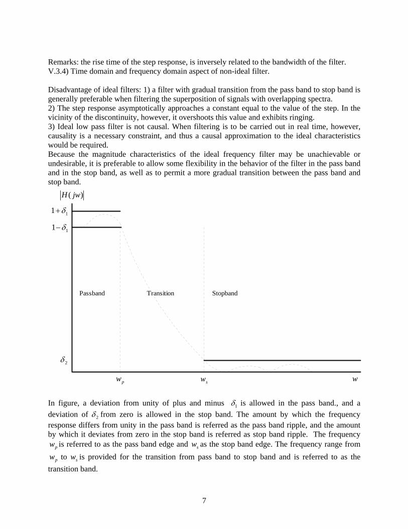
Remarks: the rise time of the step response, is inversely related to the bandwidth of the filter. V.3.4) Time domain and frequency domain aspect of non-ideal filter. Disadvantage of ideal filters: 1) a filter with gradual transition from the pass band to stop band is generally preferable when filtering the superposition of signals with overlapping spectra. 2) The step response asymptotically approaches a constant equal to the value of the step. In the vicinity of the discontinuity, however, it overshoots this value and exhibits ringing. 3) Ideal low pass filter is not causal. When filtering is to be carried out in real time, however, causality is a necessary constraint, and thus a causal approximation to the ideal characteristics would be required. Because the magnitude characteristics of the ideal frequency filter may be unachievable or undesirable, it is preferable to allow some flexibility in the behavior of the filter in the pass band and in the stop band, as well as to permit a more gradual transition between the pass band and stop band.

  pw sw w

  2δ

  11 δ−

 11 δ+

  )( jwH

Passband Transition Stopband

In figure, a deviation from unity of plus and minus 1δ is allowed in the pass band., and a deviation of 2δ from zero is allowed in the stop band. The amount by which the frequency response differs from unity in the pass band is referred as the pass band ripple, and the amount by which it deviates from zero in the stop band is referred as stop band ripple. The frequency

pw is referred to as the pass band edge and sw as the stop band edge. The frequency range from

pw to sw is provided for the transition from pass band to stop band and is referred to as the transition band.

8

Similar definitions apply to discrete-time low pass filters, as well as to other continuous and discrete time frequency selective filters. To control time-domain behavior, specifications are frequently imposed on the step response of a filter. There are rT or 1rT , pT , sT , sse

Example: 5.3 Consider an ideal high pass filter whose frequency response is specified as

⎩⎨⎧

<>

=c

c

wwww

jwH01

)(

a) Determine the impulse response t

twth c

πsin)( = for this filter.

b) As cw is increased, does )(th get more or less concentrated about the origin? c) Determine )0(s and )(∞s , where )(ts is the step response of the filter.

Solution: a) note that )(1)( 0 jwHjwH −= , where t

twthwwww

jwH c

c

c

πsin)(

01

)( 00 =↔⎩⎨⎧

>≤

=

Therefore, t

twtthtth c

πδδ sin)()()()( 0 −=−=

b) As cw is increased, )(th gets more concentrated about the origin. c) Note that the step response is given by

)()()(*)()()(*)()( 00 tstuthtutututhts −=−==

We know that 21)0(0 =s and 1)(0 =∞s

9

Therefore 21

211)0()0()0( 0 =−=−= ++ sus and 011)()()( 0 =−=∞−∞=∞ sus

V.4. First-order and second order continuous and discrete time systems

V.4.1) first order system differential equation:

)()()( txtydt

tdy=+τ

Frequency response is: 1

1)(+

=τjw

jwH

And the impulse response is )(1)( / tueth t τ

τ−=

Step response is [ ] )(1)(*)()( / tuetuthts t τ−−== Parameter τ is the time constant of the system, and it controls the rate at which the first order system responds. Example 5.4 Sketch the bode plot, and plot the impulse response and step response of following

system: 15

1)(+

=jw

jwH

-40

-30

-20

-10

0

Mag

nitu

de (d

B)

10-2

10-1

100

101

-90

-45

0

Phas

e (d

eg)

Bode Diagram

Frequency (rad/sec)

10

0 5 10 15 20 25 300

0.02

0.04

0.06

0.08

0.1

0.12

0.14

0.16

0.18

0.2Impulse Response

Time (sec)

Ampl

itude

0 5 10 15 20 25 300

0.1

0.2

0.3

0.4

0.5

0.6

0.7

0.8

0.9

1Step Response

Time (sec)

Ampl

itude

11

V.4.2) Second order continuous-time system

)()()(2)( 22 txwtywdt

tdywndt

tdynn =++ ξ

Frequency response:

( ) ( )12

12

)( 222

2

+⎟⎟⎠

⎞⎜⎜⎝

⎛+⎟⎟

⎠

⎞⎜⎜⎝

⎛=

++=

nn

nn

n

wwj

wjwwjwwjw

wjwH

ξξ

We see that the frequency response is the function of nw

w . Thus changing nw is essentially

identical to a time and frequency scaling. The parameter ξ is referred as the damping ratio and the parameter nw as the undamped natural frequency. Case 0: 0<ξ ? Case 1: 1=ξ , critical damped case

( ) ( ) ( ))()(

2)( 2

2

2

22

2

tutewthwjw

wwjwwjw

wjwH twn

n

n

nn

n n−=→+

=++

=

Step response : [ ] )(1)( tutewets tw

ntw nn −− −−=

Case 2: 1>ξ , over damped. Impulse response is the difference between two decaying exponentials. Case 3: 10 << ξ , under damped system. Use partial fraction expansion of the form

( )[ ] )(1sin1

)()( 2

221

tutwewthcjw

Mcjw

MjwH n

twn

n

ξξ

ξ

−−

=⇒−

−−

=−

Step response: )(1)(*)()(21

21

tuce

ceMtuthts

tctc

⎭⎬⎫

⎩⎨⎧

⎥⎦

⎤⎢⎣

⎡−+==

12

0 1 2 3 4 5 6 7 8 9 10-0.8

-0.6

-0.4

-0.2

0

0.2

0.4

0.6

0.8

1

ωnt

y(t)/ω

n

ζ=0.1,0.25,0.5,1.0

Impulse response

0 2 4 6 8 10 120

0.2

0.4

0.6

0.8

1

1.2

1.4

1.6

1.8

ωnt

y(t)/ω

n

ζ=0.1,0.25,0.5,1.0

Step response

13

Modern Control Systems: ELEVENTH EDITIONRichard C. Dorf and Robert H. Bishop 0-13-227028-5

Bode plot

14

V.4.3) First and second order discrete time system

a) First order discrete time system First order difference equation: ][]1[][ nxnayny =−−

With 1<a , frequency response : jwjw

aeeH −−

=1

1)(

Impulse response: ][][ nuanh n=

Step response: ][1

1][*][][1

nua

anhnunsn

−−

==+

The magnitude and phase of the first order system are:

( )21

2 cos21

1)(waa

eH jw

−+=

⎥⎦⎤

⎢⎣⎡−

−=∠ −

wawaeH jw

cos1sintan)( 1

Remarks: the magnitude of the parameter a plays a role similar to that of the time constant τ in the continuous time first order system. a determines the rate at which the first order system responds.

1) The impulse response decays sharply and the step response settles quickly for a small.

2) For a near to 1, these responses are slower. 3) When 0<a , step response exhibits both overshoot of its final value and ringing. 4) For frequency response, for 0>a , the system attenuates high frequencies. i.e., )( jweH is

smaller for w near π± than it is for w near 0. 5) For frequency response, for 0<a , the system amplifies high frequencies and attenuates

low frequencies. i.e., )( jweH is smaller for w near π2± than it is for w near π± .

Figures of frequency response and impulse response and step response see next two pages

15

-505

Mag

nitu

de (d

B)

10-1

100

101

01020

Phas

e (d

eg)

Bode Diagram

Frequency (rad/sec)

0 1 2 3 4 5 6 7 8 9 10-1

0

1Impulse Response

Time (sec)

Ampl

itude

0 1 2 3 4 5 6 7 8 9 10

0.70.80.9

Step Response

Time (sec)

Ampl

itude

a=0.25

-505

Mag

nitu

de (d

B)

10-1

100

101

01020

Phas

e (d

eg)

Bode Diagram

Frequency (rad/sec)

0 1 2 3 4 5 6 7 8 9 10-1

0

1Impulse Response

Time (sec)

Ampl

itude

0 1 2 3 4 5 6 7 8 9 10

0.70.80.9

Step Response

Time (sec)

Ampl

itude

a=-0.25

16

-200

20

Mag

nitu

de (d

B)

10-3

10-2

10-1

100

101

-90-45

0

Phas

e (d

eg)

Bode Diagram

Frequency (rad/sec)

0 5 10 15 20 25 30 35 400

0.5

1Impulse Response

Time (sec)

Ampl

itude

0 5 10 15 20 25 30 35 40 450

5

10Step Response

Time (sec)

Ampl

itude

a=7/8

-200

20

Mag

nitu

de (d

B)

10-1

100

101

04590

Phas

e (d

eg)

Bode Diagram

Frequency (rad/sec)

0 5 10 15 20 25 30 35 40-1

0

1Impulse Response

Time (sec)

Ampl

itude

0 5 10 15 20 25 30 35 40 450

0.5

1Step Response

Time (sec)

Ampl

itude

a=-7/8

17

b) Second order discrete time system

( ) ][]2[]1[cos2][ 2 nxnyrnyrny =−+−− θ With 10 << r and πθ ≤≤0 The frequency response for this system is

( )

( )[ ] ( )[ ]jwjjwj

wjjwjw

ereere

erereH

−−−

−−

−−=

+−=

θθ

θ

111

cos211)( 22

Case 1: 0≠θ or π , the two factors in the denominator of )( jweH are different, and a partial fraction expansion yields,

( )[ ] ( )[ ] ( )[ ] ( )[ ]jwjjwjjwjjwjjw

ereB

ereA

ereereeH −−−−−− −

+−

=−−

= θθθθ 11111)(

Where , θ

θ

sin2 jeA

j

= ,θ

θ

sin2 jeB

j−

=

Impulse response is ( ) ( )[ ] ( )[ ] ][sin

1sin][][ nunnrnureBreAnh nnjnj

θθθ +

=+= −

Step response: ( ) ( ) ][1

11

1][*][][11

nure

reBre

reAnhnuns j

nj

j

nj

⎥⎥⎦

⎤

⎢⎢⎣

⎡

⎟⎟⎠

⎞⎜⎜⎝

⎛

−−

+⎟⎟⎠

⎞⎜⎜⎝

⎛

−−

== −

+−+

θ

θ

θ

θ

Case 2: 0=θ or π , the two factors in the denominator of )( jweH are same,

0=θ πθ = Frequency response [ ]21

1)(jw

jw

reeH

−−= [ ]21

1)(jw

jw

reeH

−+=

Impulse response

( ) ][1][ nurnnh n+= ( )( ) ][1][ nurnnh n−+=

Step response ( ) ( ) ( ) ( ) ][1

1111

22 nurnr

rrr

rr

nn⎥⎦

⎤⎢⎣

⎡+

−+

−−

− ( ) ( )( ) ( ) ( )( ) ][1

1111

22 nurnr

rrr

rr

nn⎥⎦

⎤⎢⎣

⎡−+

+−−

++ Remarks: 1) The rate of decay of ][nh is controlled by r . The closer the r is to 1, the slower the decay in ][nh . Similarly, the value of θ determines the oscillation. With 0=θ , there is no oscillation,

πθ = there is rapid oscillation. Figures of frequency response and impulse response and step response

18

468

Mag

nitu

de (d

B)

10-2

10-1

100

101

-20-10

0

Phas

e (d

eg)

Bode Diagram

Frequency (rad/sec)

0 1 2 3 4 5 6 7 8 9 100

1

2Impulse Response

Time (sec)

Ampl

itude

0 1 2 3 4 5 6 7 8 9 102

2.5Step Response

Time (sec)

Ampl

itude

r=0.1, 0=θ

5.56

6.5

Mag

nitu

de (d

B)

10-2

10-1

100

101

-101

Phas

e (d

eg)

Bode Diagram

Frequency (rad/sec)

0 1 2 3 4 5 6 7 8 9 10-2

0

2Impulse Response

Time (sec)

Ampl

itude

0 1 2 3 4 5 6 7 8 9 101.95

2

2.05Step Response

Time (sec)

Ampl

itude

r=0.1,

2πθ =

468

Mag

nitu

de (d

B)

10-1

100

101

01020

Phas

e (d

eg)

Bode Diagram

Frequency (rad/sec)

0 1 2 3 4 5 6 7 8 9 10-2

0

2Impulse Response

Time (sec)

Ampl

itude

0 1 2 3 4 5 6 7 8 9 101.6

1.8

2Step Response

Time (sec)

Ampl

itude

r=0.1, πθ =

19

-200

20

Mag

nitu

de (d

B)

10-2

10-1

100

101

-90-45

0

Phas

e (d

eg)

Bode Diagram

Frequency (rad/sec)

0 5 10 15 20 250

1

2Impulse Response

Time (sec)

Ampl

itude

0 5 10 15 20 250

5

10Step Response

Time (sec)

Ampl

itude

r=0.5, 0=θ

05

10

Mag

nitu

de (d

B)

10-2

10-1

100

101

-200

20

Phas

e (d

eg)

Bode Diagram

Frequency (rad/sec)

0 1 2 3 4 5 6 7 8 9 10-2

0

2Impulse Response

Time (sec)

Ampl

itude

0 2 4 6 8 10 12

1.6

1.8

2Step Response

Time (sec)

Ampl

itude

r=0.5,

2πθ =

-200

20

Mag

nitu

de (d

B)

10-1

100

101

04590

Phas

e (d

eg)

Bode Diagram

Frequency (rad/sec)

0 5 10 15 20 25-2

0

2Impulse Response

Time (sec)

Ampl

itude

0 5 10 15 20 250

1

2Step Response

Time (sec)

Ampl

itude

r=0.5, πθ =

20

-500

50

Mag

nitu

de (d

B)

10-3

10-2

10-1

100

101

-180-90

0

Phas

e (d

eg)

Bode Diagram

Frequency (rad/sec)

0 10 20 30 40 50 600

5

10Impulse Response

Time (sec)

Ampl

itude

0 10 20 30 40 50 600

100

200Step Response

Time (sec)

Ampl

itude

r=0.9, 0=θ

02040

Mag

nitu

de (d

B)

10-2

10-1

100

101

-900

90

Phas

e (d

eg)

Bode Diagram

Frequency (rad/sec)

0 5 10 15 20 25 30 35 40 45-2

0

2Impulse Response

Time (sec)

Ampl

itude

0 10 20 30 40 50 600

1

2Step Response

Time (sec)

Ampl

itude

r=0.9,

2πθ =

-500

50

Mag

nitu

de (d

B)

10-1

100

101

090

180

Phas

e (d

eg)

Bode Diagram

Frequency (rad/sec)

0 10 20 30 40 50 60-10

0

10Impulse Response

Time (sec)

Ampl

itude

0 10 20 30 40 50 60-5

0

5Step Response

Time (sec)

Ampl

itude

r=0.9, πθ =

21

It is also possible to have consider the second order systems having factors with the real coefficients

( )( )jwjwjw

ededeH −− −−

=21 11

1)( , where 1d and 2d are both real numbers with 11 <d , 12 <d

( ) ][]2[]1[][ 2121 nxnyddnyddny =−+−+−

( )( ) ( ) ( )jwjwjwjwjw

edB

edA

ededeH −−−− −

+−

=−−

=2121 1111

1)( ,

Where 21

1

dddA−

= ,12

2

dddB−

=

Thus [ ] ][][ 21 nuBdAdnh nn += , which is the sum of two decaying real exponentials.

][1

11

1][*][][2

12

1

11 nu

ddB

ddAnhnuns

nn

⎥⎦

⎤⎢⎣

⎡⎟⎟⎠

⎞⎜⎜⎝

⎛−−

+⎟⎟⎠

⎞⎜⎜⎝

⎛−−

==++

V.5. Time and frequency domain analysis Example