Embed Size (px)
Citation preview
Partial Autocorrelation Function, PACF
Al NosedalUniversity of Toronto
March 5, 2019
Al Nosedal University of Toronto Partial Autocorrelation Function, PACF March 5, 2019 1 / 39
We have seen that the ACF is an excellent tool in identifying the order ofan MA(q) process, because it is expected to ”cut off” after lag q.However, we pointed out that the ACF is not as useful in the identificationof the order of an AR(p) process for which it will most likely have amixture of exponential decay and damped sinusoid expressions. Hencesuch behaviour, while indicating that the process might have an ARstructure, fails to provide further information about the order of suchstructure. For that, we will define and employ the partial autocorrelationfunction (PACF) of the time series.
Al Nosedal University of Toronto Partial Autocorrelation Function, PACF March 5, 2019 2 / 39
A reminder
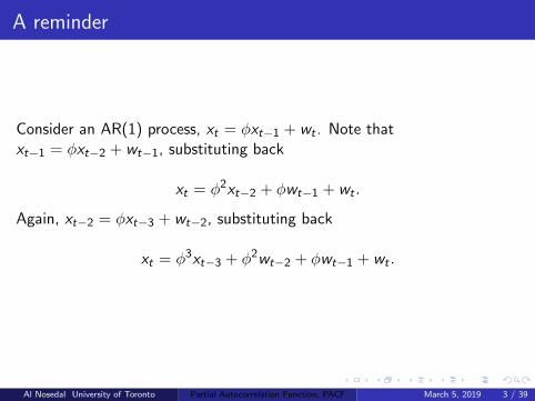
Consider an AR(1) process, xt = φxt−1 + wt . Note thatxt−1 = φxt−2 + wt−1, substituting back
xt = φ2xt−2 + φwt−1 + wt .
Again, xt−2 = φxt−3 + wt−2, substituting back
xt = φ3xt−3 + φ2wt−2 + φwt−1 + wt .
Al Nosedal University of Toronto Partial Autocorrelation Function, PACF March 5, 2019 3 / 39
A reminder
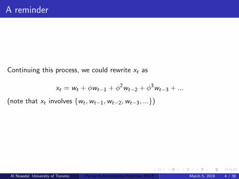
Continuing this process, we could rewrite xt as
xt = wt + φwt−1 + φ2wt−2 + φ3wt−3 + ...
(note that xt involves {wt ,wt−1,wt−2,wt−3, ...})
Al Nosedal University of Toronto Partial Autocorrelation Function, PACF March 5, 2019 4 / 39
PACF
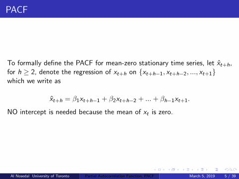
To formally define the PACF for mean-zero stationary time series, let x̂t+h,for h ≥ 2, denote the regression of xt+h on {xt+h−1, xt+h−2, ..., xt+1}which we write as
x̂t+h = β1xt+h−1 + β2xt+h−2 + ...+ βh−1xt+1.
NO intercept is needed because the mean of xt is zero.
Al Nosedal University of Toronto Partial Autocorrelation Function, PACF March 5, 2019 5 / 39
PACF
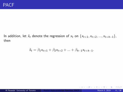
In addition, let x̂t denote the regression of xt on {xt+1, xt+2, ..., xt+h−1},then
x̂t = β1xt+1 + β2xt+2 + ...+ βh−1xt+h−1.
Al Nosedal University of Toronto Partial Autocorrelation Function, PACF March 5, 2019 6 / 39
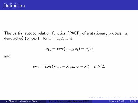
Definition
The partial autocorrelation function (PACF) of a stationary process, xt ,denoted φhh (or φhh) , for h = 1, 2, ... is
φ11 = corr(xt+1, xt) = ρ(1)
and
φhh = corr(xt+h − x̂t+h, xt − x̂t), h ≥ 2.
Al Nosedal University of Toronto Partial Autocorrelation Function, PACF March 5, 2019 7 / 39
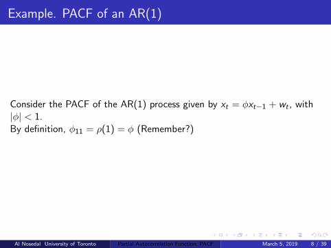
Example. PACF of an AR(1)
Consider the PACF of the AR(1) process given by xt = φxt−1 + wt , with|φ| < 1.By definition, φ11 = ρ(1) = φ (Remember?)
Al Nosedal University of Toronto Partial Autocorrelation Function, PACF March 5, 2019 8 / 39
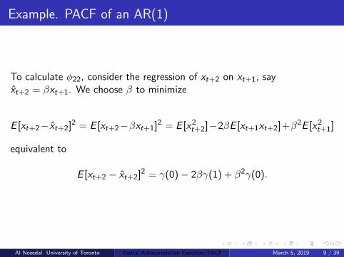
Example. PACF of an AR(1)
To calculate φ22, consider the regression of xt+2 on xt+1, sayx̂t+2 = βxt+1. We choose β to minimize
E [xt+2− x̂t+2]2 = E [xt+2−βxt+1]2 = E [x2t+2]−2βE [xt+1xt+2]+β2E [x2t+1]
equivalent to
E [xt+2 − x̂t+2]2 = γ(0)− 2βγ(1) + β2γ(0).
Al Nosedal University of Toronto Partial Autocorrelation Function, PACF March 5, 2019 9 / 39
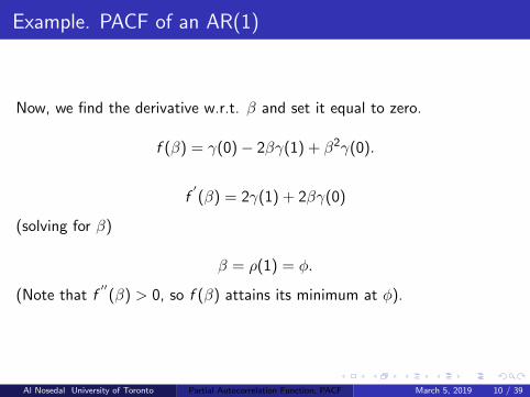
Example. PACF of an AR(1)
Now, we find the derivative w.r.t. β and set it equal to zero.
f (β) = γ(0)− 2βγ(1) + β2γ(0).
f′(β) = 2γ(1) + 2βγ(0)
(solving for β)
β = ρ(1) = φ.
(Note that f′′
(β) > 0, so f (β) attains its minimum at φ).
Al Nosedal University of Toronto Partial Autocorrelation Function, PACF March 5, 2019 10 / 39

Example. PACF of an AR(1)
Next, consider the regression of xt on xt+1, say x̂t = βxt+1. We choose βto minimize
E [xt − x̂t ]2 = E [xt − βxt+1]2 = E [x2t ]− 2βE [xtxt+1] + β2E [x2t+1]
equivalent to
E [xt − x̂t ]2 = γ(0)− 2βγ(1) + β2γ(0).
This is the same equation as before, so β = ρ(1) = φ.
Al Nosedal University of Toronto Partial Autocorrelation Function, PACF March 5, 2019 11 / 39
Example. PACF of an AR(1)
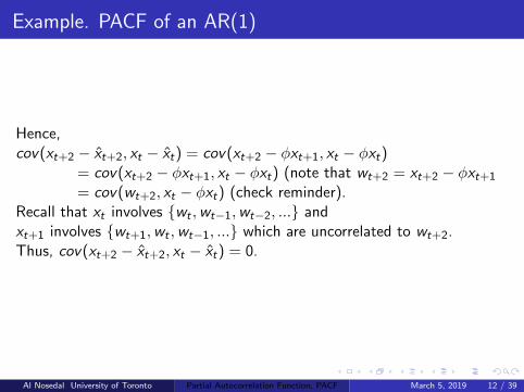
Hence,cov(xt+2 − x̂t+2, xt − x̂t) = cov(xt+2 − φxt+1, xt − φxt)
= cov(xt+2 − φxt+1, xt − φxt) (note that wt+2 = xt+2 − φxt+1
= cov(wt+2, xt − φxt) (check reminder).Recall that xt involves {wt ,wt−1,wt−2, ...} andxt+1 involves {wt+1,wt ,wt−1, ...} which are uncorrelated to wt+2.Thus, cov(xt+2 − x̂t+2, xt − x̂t) = 0.
Al Nosedal University of Toronto Partial Autocorrelation Function, PACF March 5, 2019 12 / 39
Example. PACF of an AR(1)
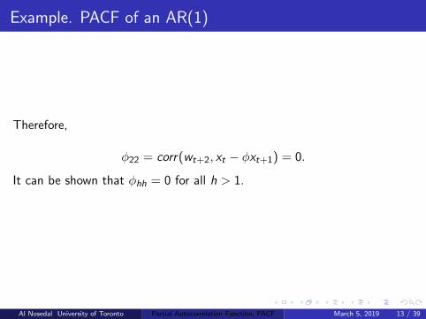
Therefore,
φ22 = corr(wt+2, xt − φxt+1) = 0.
It can be shown that φhh = 0 for all h > 1.
Al Nosedal University of Toronto Partial Autocorrelation Function, PACF March 5, 2019 13 / 39
What is the PACF
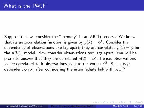
Suppose that we consider the ”memory” in an AR(1) process. We knowthat its autocorrelation function is given by ρ(k) = φk . Consider thedependency of observations one lag apart; they are correlated ρ(1) = φ forthe AR(1) model. Now consider observations two lags apart. You will beprone to answer that they are correlated ρ(2) = φ2. Hence, observationsxt are correlated with observations xt+2 to the extent φ2. But is xt+2
dependent on xt after considering the intermediate link with xt+1?
Al Nosedal University of Toronto Partial Autocorrelation Function, PACF March 5, 2019 14 / 39
What is the PACF
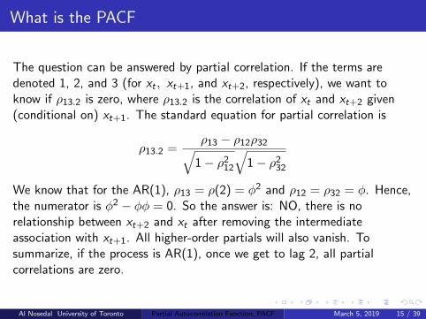
The question can be answered by partial correlation. If the terms aredenoted 1, 2, and 3 (for xt , xt+1, and xt+2, respectively), we want toknow if ρ13.2 is zero, where ρ13.2 is the correlation of xt and xt+2 given(conditional on) xt+1. The standard equation for partial correlation is
ρ13.2 =ρ13 − ρ12ρ32√
1− ρ212√
1− ρ232
We know that for the AR(1), ρ13 = ρ(2) = φ2 and ρ12 = ρ32 = φ. Hence,the numerator is φ2 − φφ = 0. So the answer is: NO, there is norelationship between xt+2 and xt after removing the intermediateassociation with xt+1. All higher-order partials will also vanish. Tosummarize, if the process is AR(1), once we get to lag 2, all partialcorrelations are zero.
Al Nosedal University of Toronto Partial Autocorrelation Function, PACF March 5, 2019 15 / 39
Example: Applying the Yule-Walker Equations
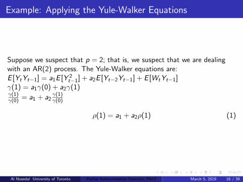
Suppose we suspect that p = 2; that is, we suspect that we are dealingwith an AR(2) process. The Yule-Walker equations are:E [YtYt−1] = a1E [Y 2
t−1] + a2E [Yt−2Yt−1] + E [WtYt−1]γ(1) = a1γ(0) + a2γ(1)γ(1)γ(0) = a1 + a2
γ(1)γ(0)
ρ(1) = a1 + a2ρ(1) (1)
Al Nosedal University of Toronto Partial Autocorrelation Function, PACF March 5, 2019 16 / 39
Example: Applying the Yule-Walker Equations (cont.)
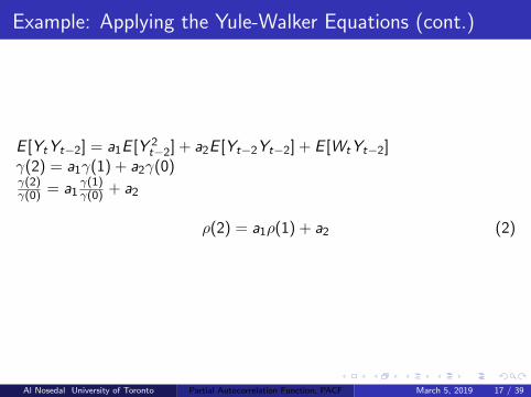
E [YtYt−2] = a1E [Y 2t−2] + a2E [Yt−2Yt−2] + E [WtYt−2]
γ(2) = a1γ(1) + a2γ(0)γ(2)γ(0) = a1
γ(1)γ(0) + a2
ρ(2) = a1ρ(1) + a2 (2)
Al Nosedal University of Toronto Partial Autocorrelation Function, PACF March 5, 2019 17 / 39
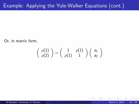
Example: Applying the Yule-Walker Equations (cont.)
Or, in matrix form,(ρ(1)ρ(2)
)=
(1 ρ(1)ρ(1) 1
)(a1a2
)
Al Nosedal University of Toronto Partial Autocorrelation Function, PACF March 5, 2019 18 / 39
Example: Applying the Yule-Walker Equations (cont.)
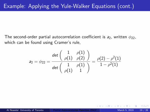
The second-order partial autocorrelation coefficient is a2, written φ22,which can be found using Cramer’s rule,
a2 = φ22 =
det
(1 ρ(1)ρ(1) ρ(2)
)det
(1 ρ(1)ρ(1) 1
) =ρ(2)− ρ2(1)
1− ρ2(1)
Al Nosedal University of Toronto Partial Autocorrelation Function, PACF March 5, 2019 19 / 39
Example
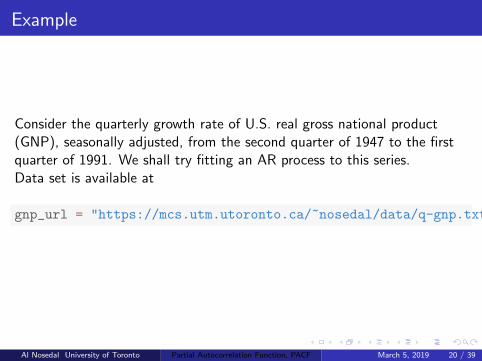
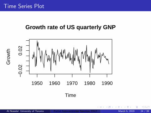
Consider the quarterly growth rate of U.S. real gross national product(GNP), seasonally adjusted, from the second quarter of 1947 to the firstquarter of 1991. We shall try fitting an AR process to this series.Data set is available at
gnp_url = "https://mcs.utm.utoronto.ca/~nosedal/data/q-gnp.txt"
Al Nosedal University of Toronto Partial Autocorrelation Function, PACF March 5, 2019 20 / 39
R Code
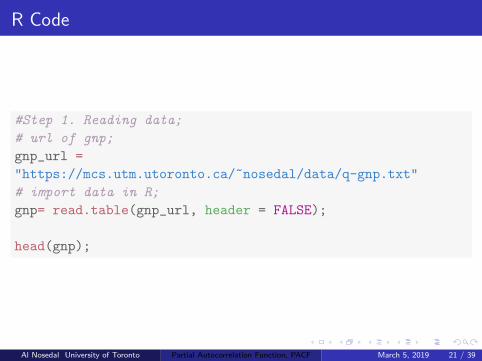
#Step 1. Reading data;
# url of gnp;
gnp_url =
"https://mcs.utm.utoronto.ca/~nosedal/data/q-gnp.txt"
# import data in R;
gnp= read.table(gnp_url, header = FALSE);
head(gnp);
Al Nosedal University of Toronto Partial Autocorrelation Function, PACF March 5, 2019 21 / 39
R Code
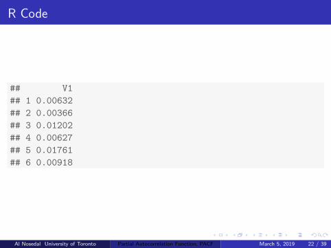
## V1
## 1 0.00632
## 2 0.00366
## 3 0.01202
## 4 0.00627
## 5 0.01761
## 6 0.00918
Al Nosedal University of Toronto Partial Autocorrelation Function, PACF March 5, 2019 22 / 39
Time Series Plot
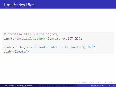
# creating time series object;
gnp.ts=ts(gnp,frequency=4,start=c(1947,2));
plot(gnp.ts,main="Growth rate of US quarterly GNP",
ylab="Growth");
Al Nosedal University of Toronto Partial Autocorrelation Function, PACF March 5, 2019 23 / 39
Time Series Plot
Growth rate of US quarterly GNP
Time
Gro
wth
1950 1960 1970 1980 1990
−0.
020.
02
Al Nosedal University of Toronto Partial Autocorrelation Function, PACF March 5, 2019 24 / 39
ACF
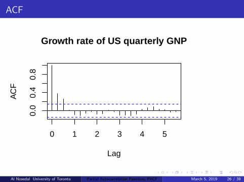
acf(gnp.ts,main="Growth rate of US quarterly GNP");
Al Nosedal University of Toronto Partial Autocorrelation Function, PACF March 5, 2019 25 / 39
ACF
0 1 2 3 4 5
0.0
0.4
0.8
Lag
AC
F
Growth rate of US quarterly GNP
Al Nosedal University of Toronto Partial Autocorrelation Function, PACF March 5, 2019 26 / 39
Autocorrelations (values)
rhos=acf(gnp.ts,plot=FALSE)$acf;
rhos[1];
rhos[2];
rhos[3];
rhos[4];
Al Nosedal University of Toronto Partial Autocorrelation Function, PACF March 5, 2019 27 / 39
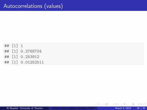
Autocorrelations (values)
## [1] 1
## [1] 0.3768704
## [1] 0.253912
## [1] 0.01252511
Al Nosedal University of Toronto Partial Autocorrelation Function, PACF March 5, 2019 28 / 39
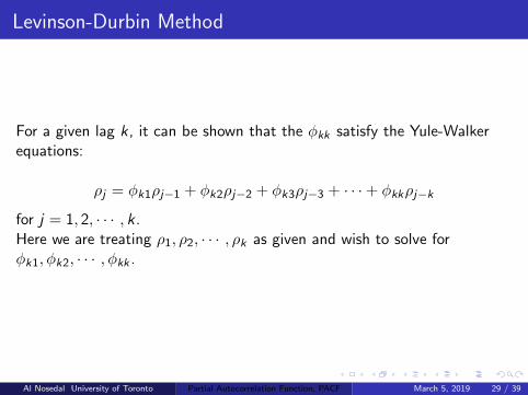
Levinson-Durbin Method
For a given lag k, it can be shown that the φkk satisfy the Yule-Walkerequations:
ρj = φk1ρj−1 + φk2ρj−2 + φk3ρj−3 + · · ·+ φkkρj−k
for j = 1, 2, · · · , k .Here we are treating ρ1, ρ2, · · · , ρk as given and wish to solve forφk1, φk2, · · · , φkk .
Al Nosedal University of Toronto Partial Autocorrelation Function, PACF March 5, 2019 29 / 39
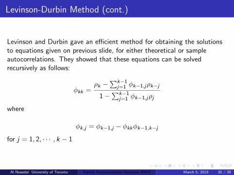
Levinson-Durbin Method (cont.)
Levinson and Durbin gave an efficient method for obtaining the solutionsto equations given on previous slide, for either theoretical or sampleautocorrelations. They showed that these equations can be solvedrecursively as follows:
φkk =ρk −
∑k−1j=1 φk−1,jρk−j
1−∑k−1
j=1 φk−1,jρj
where
φk,j = φk−1,j − φkkφk−1,k−j
for j = 1, 2, · · · , k − 1
Al Nosedal University of Toronto Partial Autocorrelation Function, PACF March 5, 2019 30 / 39
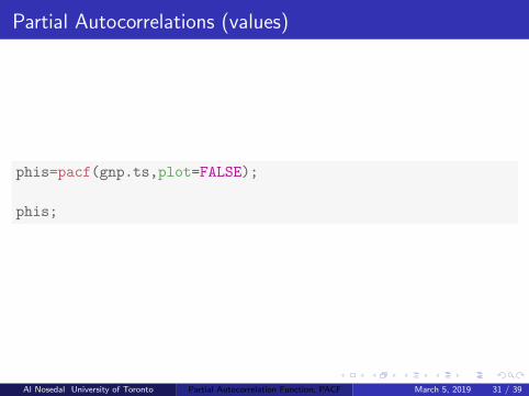
Partial Autocorrelations (values)
phis=pacf(gnp.ts,plot=FALSE);
phis;
Al Nosedal University of Toronto Partial Autocorrelation Function, PACF March 5, 2019 31 / 39
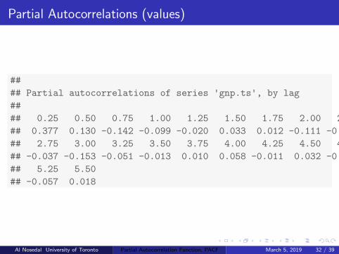
Partial Autocorrelations (values)
##
## Partial autocorrelations of series 'gnp.ts', by lag
##
## 0.25 0.50 0.75 1.00 1.25 1.50 1.75 2.00 2.25 2.50
## 0.377 0.130 -0.142 -0.099 -0.020 0.033 0.012 -0.111 -0.042 0.098
## 2.75 3.00 3.25 3.50 3.75 4.00 4.25 4.50 4.75 5.00
## -0.037 -0.153 -0.051 -0.013 0.010 0.058 -0.011 0.032 -0.017 -0.016
## 5.25 5.50
## -0.057 0.018
Al Nosedal University of Toronto Partial Autocorrelation Function, PACF March 5, 2019 32 / 39

PACF
pacf(gnp.ts,main="Growth rate of US quarterly GNP");
Al Nosedal University of Toronto Partial Autocorrelation Function, PACF March 5, 2019 33 / 39
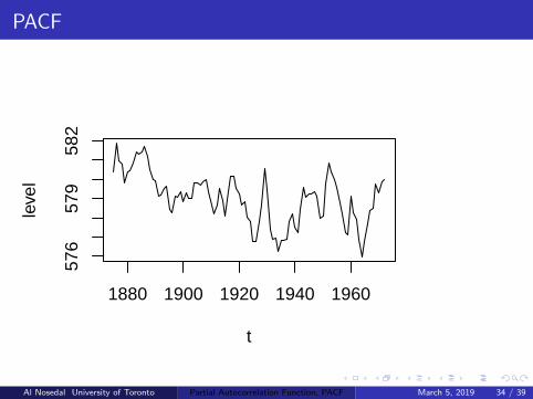
PACF
t
leve
l
1880 1900 1920 1940 1960
576
579
582
Al Nosedal University of Toronto Partial Autocorrelation Function, PACF March 5, 2019 34 / 39
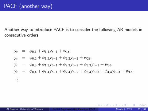
PACF (another way)
Another way to introduce PACF is to consider the following AR models inconsecutive orders:
yt = φ0,1 + φ1,1yt−1 + w1t ,
yt = φ0,2 + φ1,2yt−1 + φ2,2yt−2 + w2t ,
yt = φ0,3 + φ1,3yt−1 + φ2,3yt−2 + φ3,3yt−3 + w3t ,
yt = φ0,4 + φ1,4yt−1 + φ2,4yt−2 + φ3,4yt−3 + φ4,4yt−3 + w4t ,
...
Al Nosedal University of Toronto Partial Autocorrelation Function, PACF March 5, 2019 35 / 39
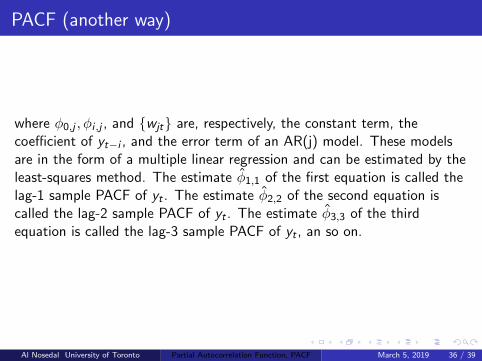
PACF (another way)
where φ0,j , φi ,j , and {wjt} are, respectively, the constant term, thecoefficient of yt−i , and the error term of an AR(j) model. These modelsare in the form of a multiple linear regression and can be estimated by theleast-squares method. The estimate φ̂1,1 of the first equation is called thelag-1 sample PACF of yt . The estimate φ̂2,2 of the second equation iscalled the lag-2 sample PACF of yt . The estimate φ̂3,3 of the thirdequation is called the lag-3 sample PACF of yt , an so on.
Al Nosedal University of Toronto Partial Autocorrelation Function, PACF March 5, 2019 36 / 39
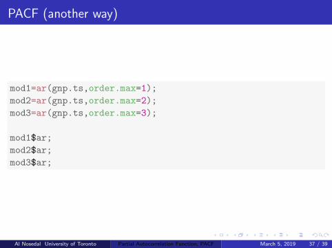
PACF (another way)
mod1=ar(gnp.ts,order.max=1);
mod2=ar(gnp.ts,order.max=2);
mod3=ar(gnp.ts,order.max=3);
mod1$ar;
mod2$ar;
mod3$ar;
Al Nosedal University of Toronto Partial Autocorrelation Function, PACF March 5, 2019 37 / 39
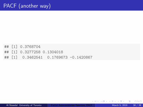
PACF (another way)
## [1] 0.3768704
## [1] 0.3277258 0.1304018
## [1] 0.3462541 0.1769673 -0.1420867
Al Nosedal University of Toronto Partial Autocorrelation Function, PACF March 5, 2019 38 / 39
For a stationary Gaussian AR(p) model, it can be shown that the samplePACF has the following properties:
φ̂p,p converges to φp as the sample size T goes to infinity.
φ̂l ,l converges to zero for all l > p.
The asymptotic variance of φ̂l ,l is 1T for l > p.
These results say that, for an AR(p) series, the sample PACF cuts off atlag p.
Al Nosedal University of Toronto Partial Autocorrelation Function, PACF March 5, 2019 39 / 39