Embed Size (px)
Citation preview
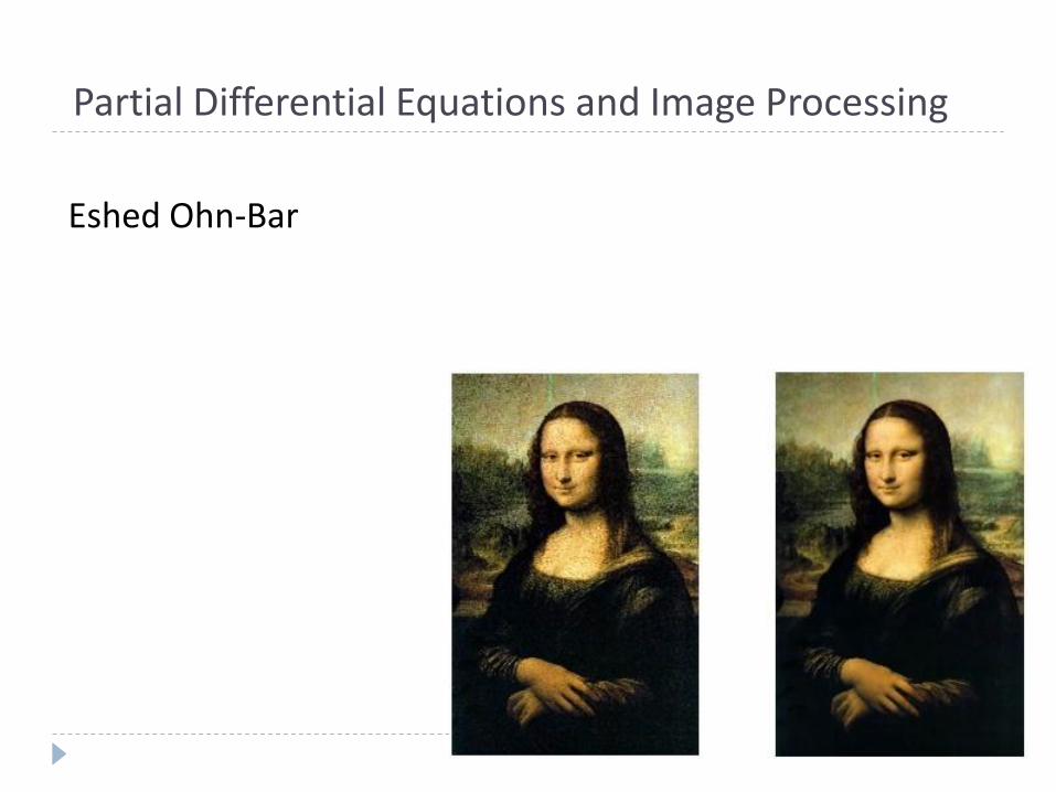
Partial Differential Equations and Image Processing
Eshed Ohn-Bar
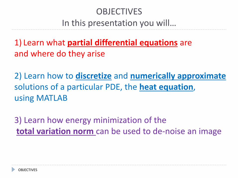
OBJECTIVES In this presentation you will…
1) Learn what partial differential equations are and where do they arise
2) Learn how to discretize and numerically approximate solutions of a particular PDE, the heat equation, using MATLAB 3) Learn how energy minimization of the total variation norm can be used to de-noise an image
OBJECTIVES
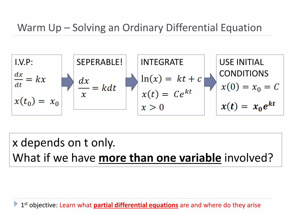
Warm Up – Solving an Ordinary Differential Equation
x depends on t only. What if we have more than one variable involved?
1st objective: Learn what partial differential equations are and where do they arise
I.V.P:
SEPERABLE!
INTEGRATE
USE INITIAL CONDITIONS
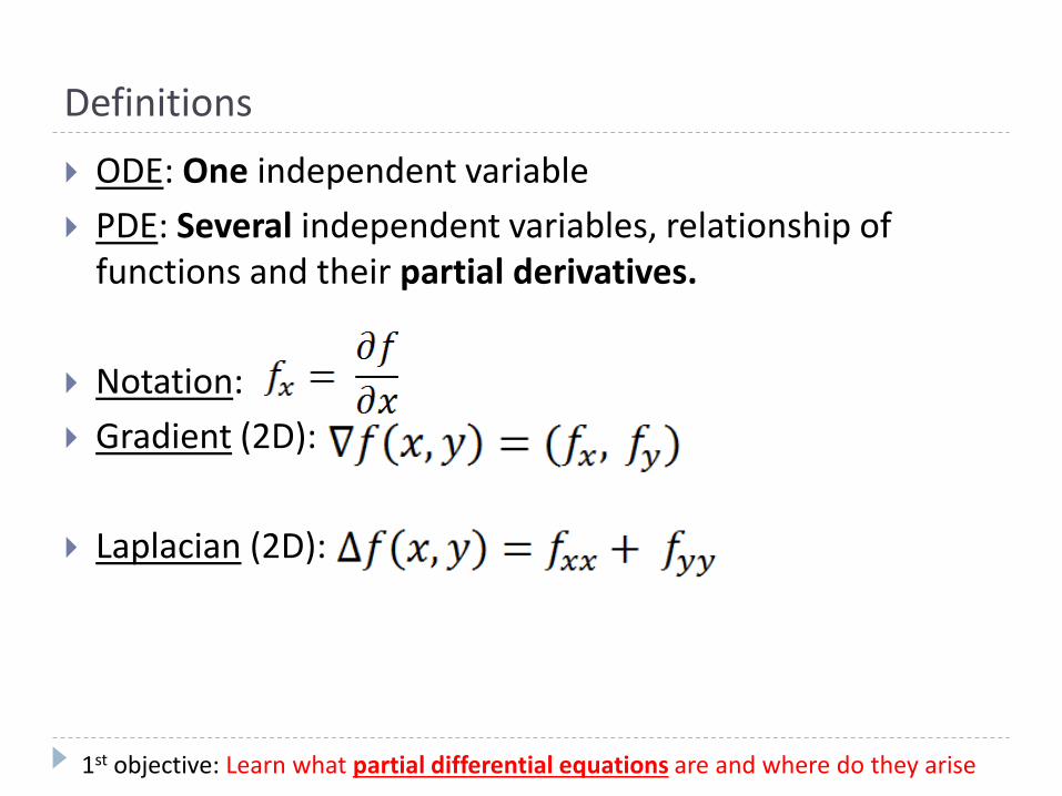
Definitions
ODE: One independent variable
PDE: Several independent variables, relationship of functions and their partial derivatives.
Notation:
Gradient (2D):
Laplacian (2D):
1st objective: Learn what partial differential equations are and where do they arise
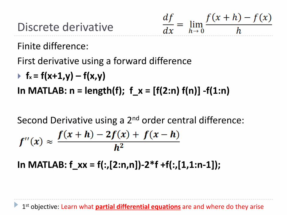
Discrete derivative
Finite difference:
First derivative using a forward difference
fx = f(x+1,y) – f(x,y)
In MATLAB: n = length(f); f_x = [f(2:n) f(n)] -f(1:n)
Second Derivative using a 2nd order central difference:
In MATLAB: f_xx = f(:,[2:n,n])-2*f +f(:,[1,1:n-1]);
1st objective: Learn what partial differential equations are and where do they arise
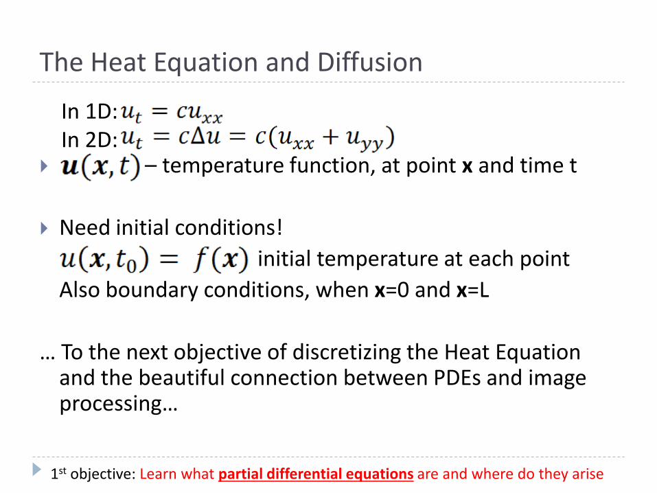
The Heat Equation and Diffusion
– temperature function, at point x and time t
Need initial conditions!
initial temperature at each point
Also boundary conditions, when x=0 and x=L
… To the next objective of discretizing the Heat Equation and the beautiful connection between PDEs and image processing…
In 1D: In 2D:
1st objective: Learn what partial differential equations are and where do they arise
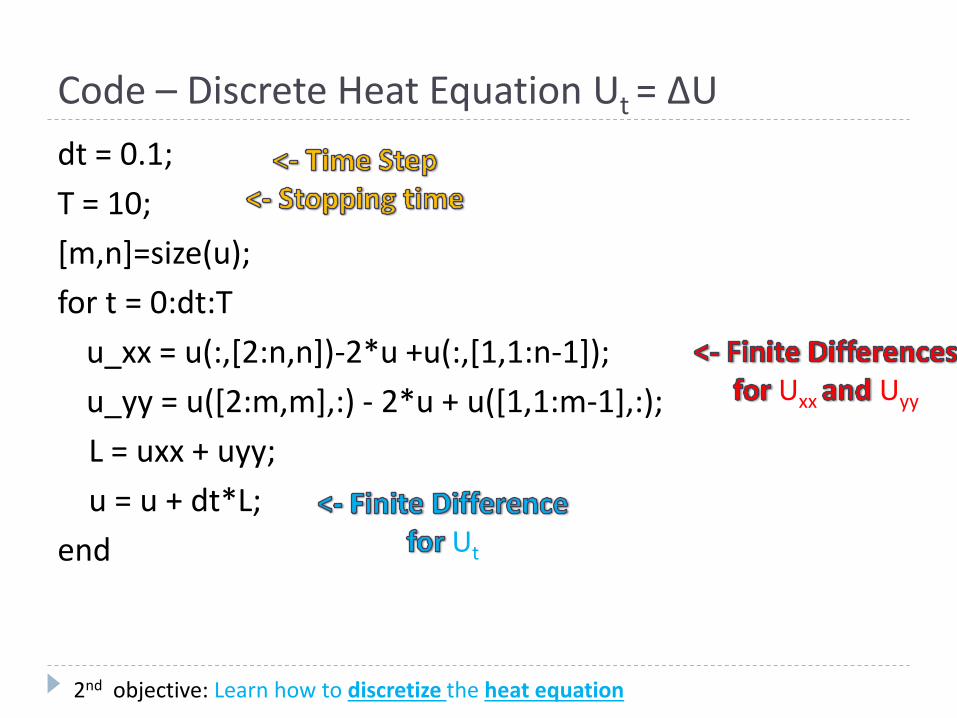
Code – Discrete Heat Equation Ut = ΔU
dt = 0.1;
T = 10;
[m,n]=size(u);
for t = 0:dt:T
u_xx = u(:,[2:n,n])-2*u +u(:,[1,1:n-1]);
u_yy = u([2:m,m],:) - 2*u + u([1,1:m-1],:);
L = uxx + uyy;
u = u + dt*L;
end
2nd objective: Learn how to discretize the heat equation
Uxx Uyy
Ut
Heat Equation on an Image
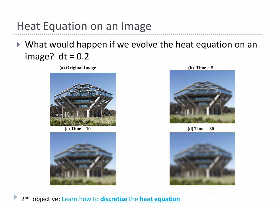
What would happen if we evolve the heat equation on an image? dt = 0.2
2nd objective: Learn how to discretize the heat equation
(a) Original Image (b) Time = 5
(c) Time = 10 (d) Time = 30
Heat Equation on an Image
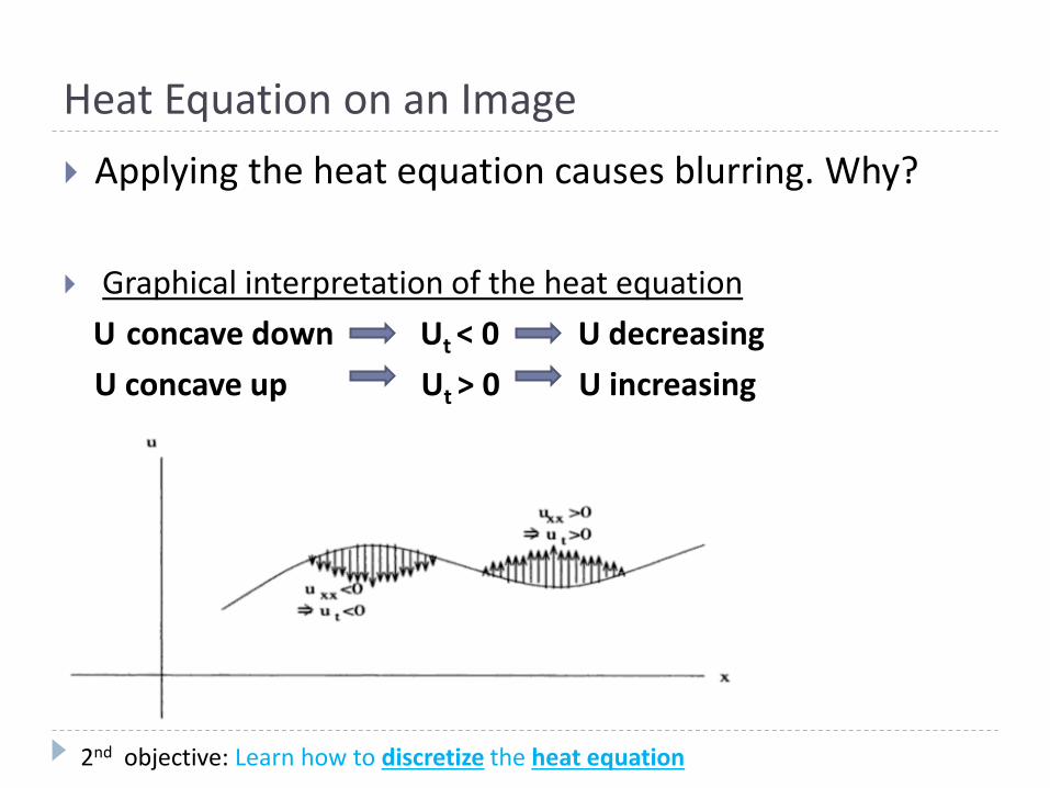
Applying the heat equation causes blurring. Why?
Graphical interpretation of the heat equation
U concave down Ut < 0 U decreasing
U concave up Ut > 0 U increasing
2nd objective: Learn how to discretize the heat equation
Heat Equation on an Image
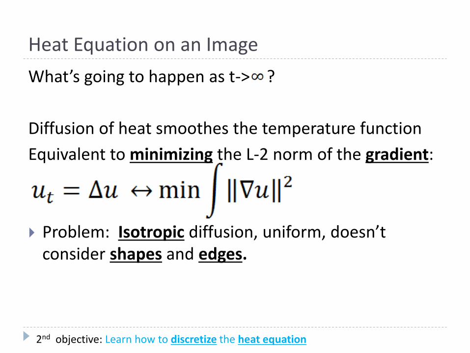
What’s going to happen as t-> ?
Diffusion of heat smoothes the temperature function
Equivalent to minimizing the L-2 norm of the gradient:
Problem: Isotropic diffusion, uniform, doesn’t consider shapes and edges.
2nd objective: Learn how to discretize the heat equation
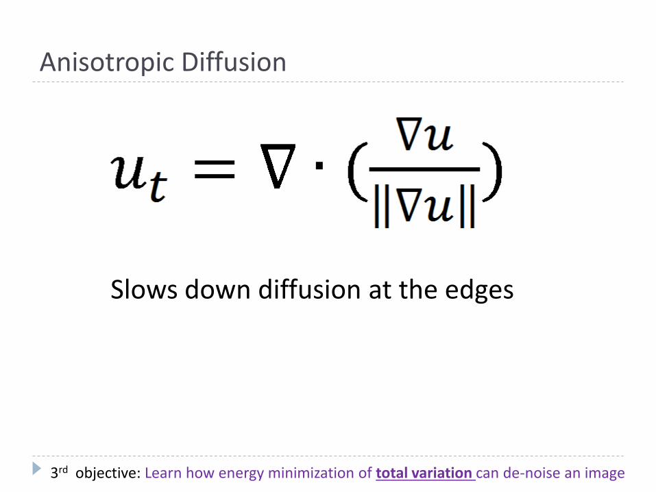
Anisotropic Diffusion
Slows down diffusion at the edges
3rd objective: Learn how energy minimization of total variation can de-noise an image
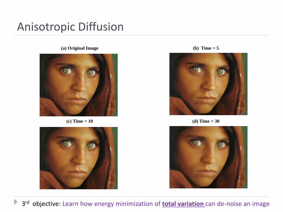
Anisotropic Diffusion
(a) Original Image (b) Time = 5
(c) Time = 10 (d) Time = 30
3rd objective: Learn how energy minimization of total variation can de-noise an image
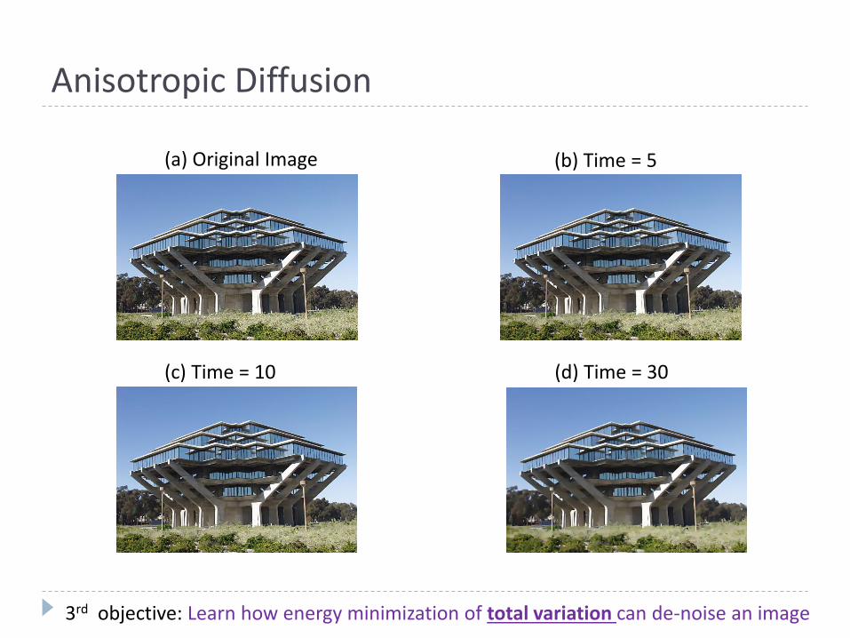
Anisotropic Diffusion
3rd objective: Learn how energy minimization of total variation can de-noise an image
(a) Original Image (b) Time = 5
(c) Time = 10 (d) Time = 30
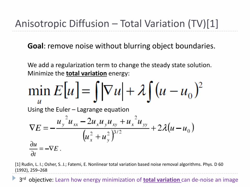
Anisotropic Diffusion – Total Variation (TV)[1]
3rd objective: Learn how energy minimization of total variation can de-noise an image
[1] Rudin, L. I.; Osher, S. J.; Fatemi, E. Nonlinear total variation based noise removal algorithms. Phys. D 60 (1992), 259–268
Goal: remove noise without blurring object boundaries. We add a regularization term to change the steady state solution. Minimize the total variation energy:
Using the Euler – Lagrange equation
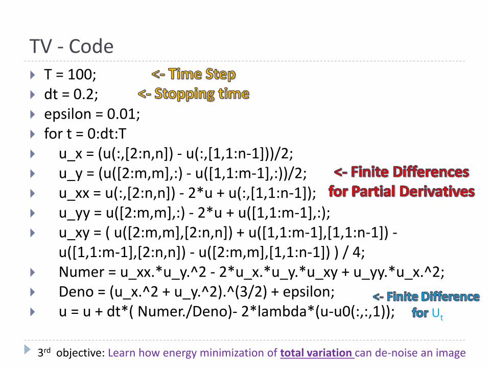
TV - Code T = 100; dt = 0.2; epsilon = 0.01; for t = 0:dt:T u_x = (u(:,[2:n,n]) - u(:,[1,1:n-1]))/2; u_y = (u([2:m,m],:) - u([1,1:m-1],:))/2; u_xx = u(:,[2:n,n]) - 2*u + u(:,[1,1:n-1]); u_yy = u([2:m,m],:) - 2*u + u([1,1:m-1],:); u_xy = ( u([2:m,m],[2:n,n]) + u([1,1:m-1],[1,1:n-1]) - u([1,1:m-1],[2:n,n]) - u([2:m,m],[1,1:n-1]) ) / 4; Numer = u_xx.*u_y.^2 - 2*u_x.*u_y.*u_xy + u_yy.*u_x.^2; Deno = (u_x.^2 + u_y.^2).^(3/2) + epsilon; u = u + dt*( Numer./Deno)- 2*lambda*(u-u0(:,:,1));
Ut
3rd objective: Learn how energy minimization of total variation can de-noise an image
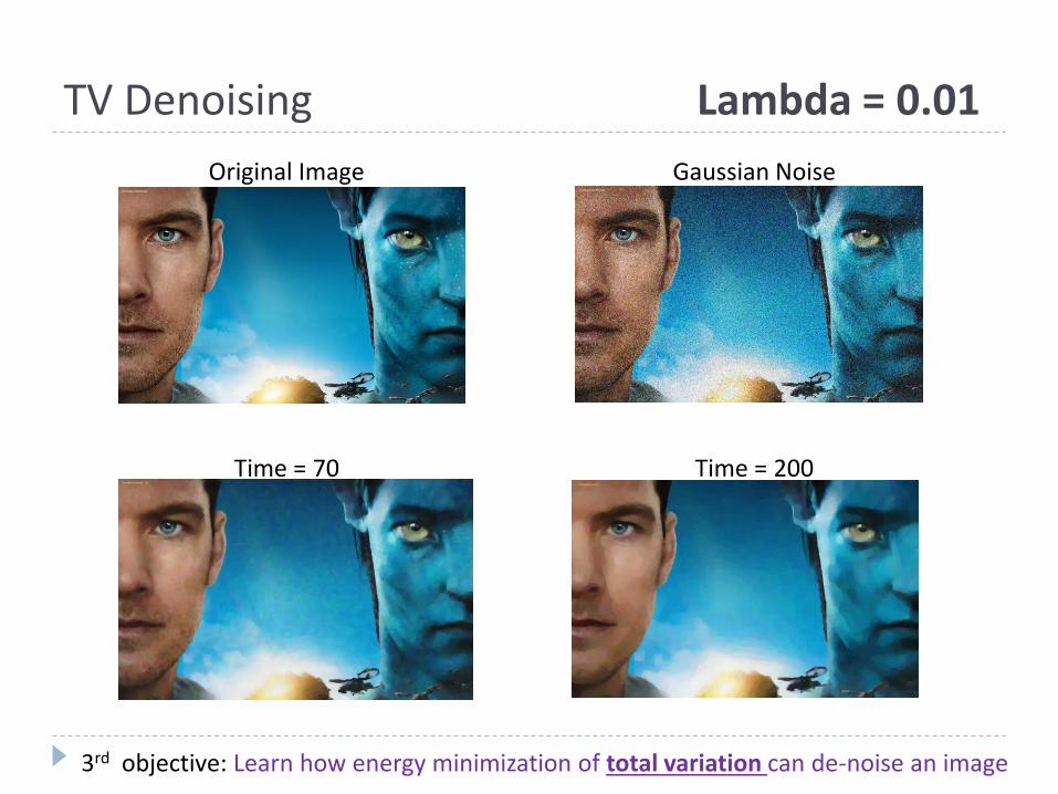
TV Denoising Lambda = 0.01
Original Image
Gaussian Noise
Time = 70 Time = 200
3rd objective: Learn how energy minimization of total variation can de-noise an image
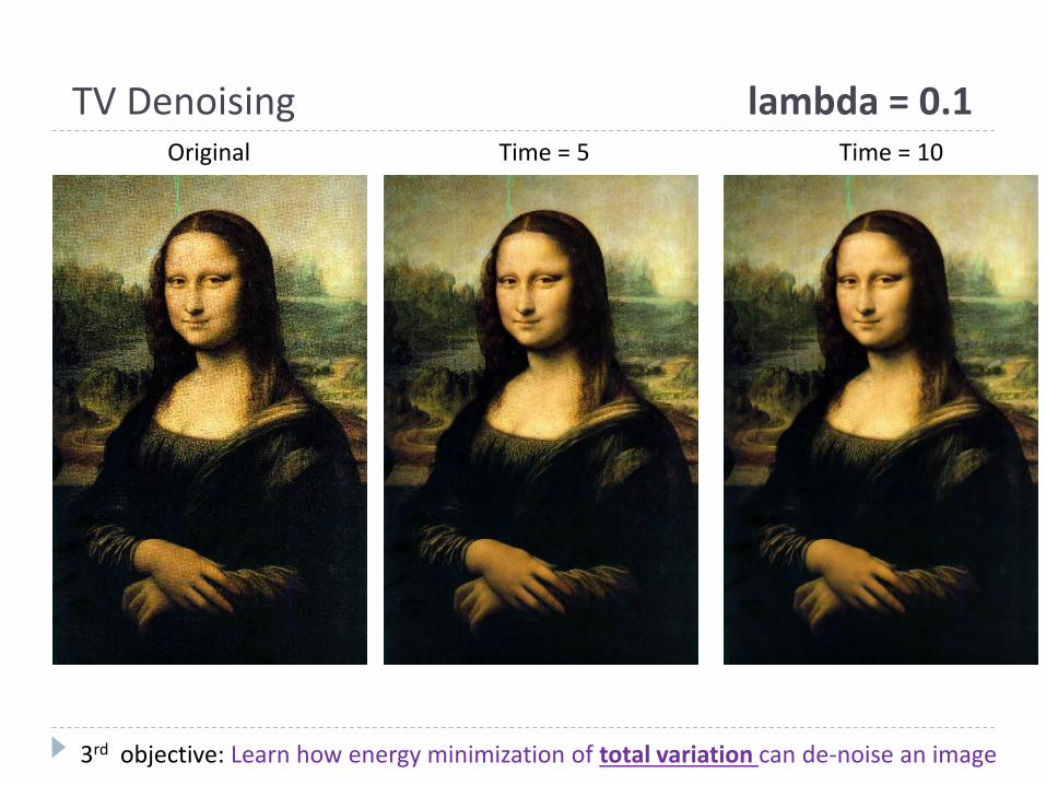
TV Denoising lambda = 0.1
3rd objective: Learn how energy minimization of total variation can de-noise an image
Original Time = 5 Time = 10
How to choose Lambda?
There are various optimization and ad-hoc methods, beyond the scope of this project.
In this project, the value is determined by pleasing results.
Lambda too large -> may not remove all the noise in the image.
Lambda too small -> it may distort important features from the image.
3rd objective: Learn how energy minimization of total variation can de-noise an image
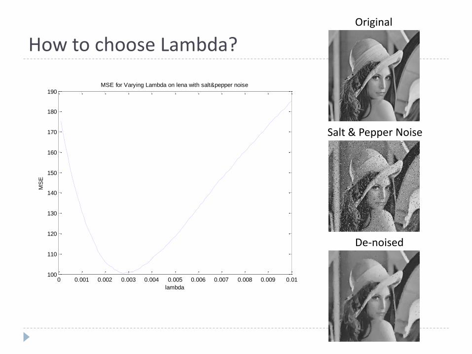
How to choose Lambda?
0 0.001 0.002 0.003 0.004 0.005 0.006 0.007 0.008 0.009 0.01100
110
120
130
140
150
160
170
180
190
lambda
MS
E
MSE for Varying Lambda on lena with salt&pepper noise
Original
Salt & Pepper Noise
De-noised
Summary
Energy minimization problems can be translated to a PDE and applied to de-noise images
We can use the magnitude of the gradient to produce anisotropic diffusion that preserves edges
TV energy minimization uses the L1-norm of the gradient, which produces nicer results on images than the L2-norm