Embed Size (px)
Citation preview
1
Lecture 11 • 1
6.825 Techniques in Artificial Intelligence
Partial-Order Planning Algorithms
Last time we talked about partial order planning, and we got through the basic idea and the formal description of what constituted a solution. So, our plan for today is to actually write the algorithm, and then go back and work through the example that we did, especially the last part of it and be sure we see how the algorithm would do the steps that are necessary to get the plan steps to come out in the right order, and to do another example just for practice. Then, next time, we’ll talk about a newer algorithm called GraphPlan.

2
Lecture 11 • 2
Partially Ordered Plan
• Plan• Steps• Ordering constraints• Variable binding constraints• Causal links
Let’s just briefly review the parts of a partially ordered plan. There are the steps, or actions we plan to take. There are ordering constraints that say which steps have to be before which other ones. They need to be consistent, but they don’t need to specify a total order on the steps. There are variable binding constraints that specify which variables are equal to which other variables or constants. And there are causal links to remind us which effects of actions we are using to satisfy which preconditions of other actions.
3
Lecture 11 • 3
Partially Ordered Plan
• Plan• Steps• Ordering constraints• Variable binding constraints• Causal links
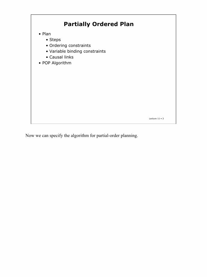
• POP Algorithm
Now we can specify the algorithm for partial-order planning.
4
Lecture 11 • 4
Partially Ordered Plan
• Plan• Steps• Ordering constraints• Variable binding constraints• Causal links
• POP Algorithm• Make initial plan start
finish
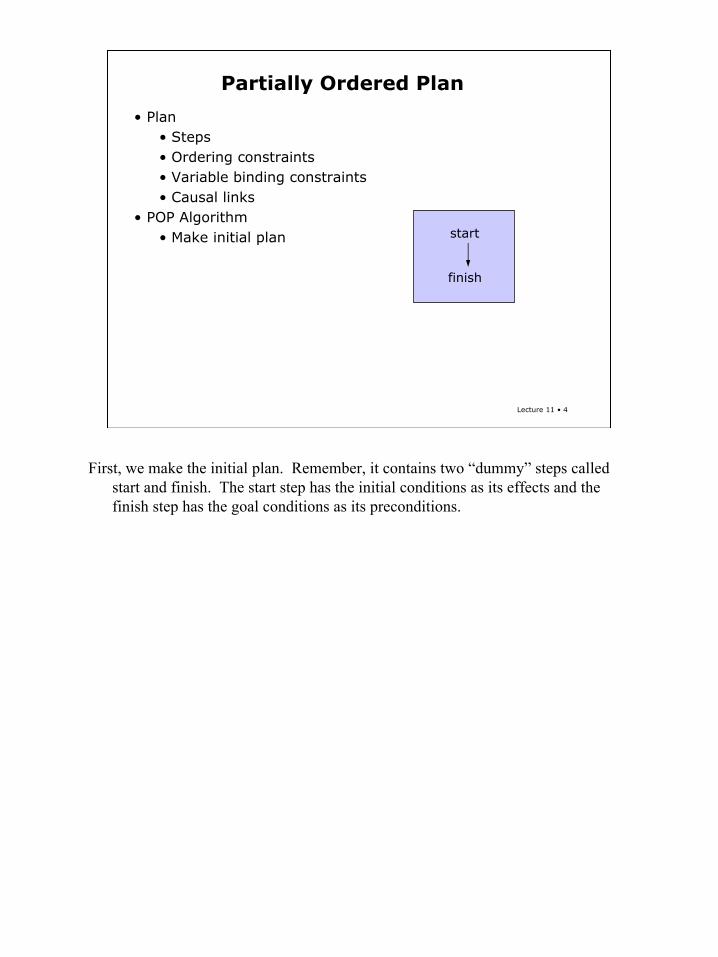
First, we make the initial plan. Remember, it contains two “dummy” steps called start and finish. The start step has the initial conditions as its effects and the finish step has the goal conditions as its preconditions.
5
Lecture 11 • 5
Partially Ordered Plan
• Plan• Steps• Ordering constraints• Variable binding constraints• Causal links
• POP Algorithm• Make initial plan
• Loop until plan is a complete
start
finish
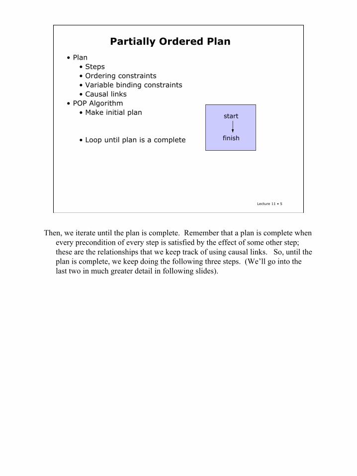
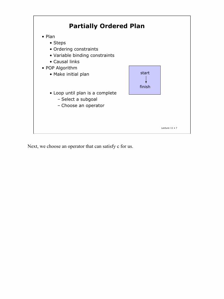
Then, we iterate until the plan is complete. Remember that a plan is complete when every precondition of every step is satisfied by the effect of some other step; these are the relationships that we keep track of using causal links. So, until the plan is complete, we keep doing the following three steps. (We’ll go into the last two in much greater detail in following slides).
6
Lecture 11 • 6
Partially Ordered Plan
• Plan• Steps• Ordering constraints• Variable binding constraints• Causal links
• POP Algorithm• Make initial plan
• Loop until plan is a complete– Select a subgoal
start
finish
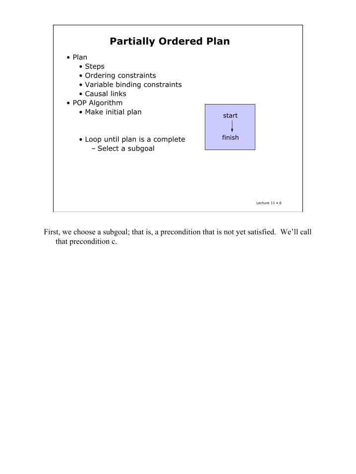
First, we choose a subgoal; that is, a precondition that is not yet satisfied. We’ll callthat precondition c.
7
Lecture 11 • 7
Partially Ordered Plan
• Plan• Steps• Ordering constraints• Variable binding constraints• Causal links
• POP Algorithm• Make initial plan
• Loop until plan is a complete– Select a subgoal– Choose an operator
start
finish
Next, we choose an operator that can satisfy c for us.
8
Lecture 11 • 8
Partially Ordered Plan
• Plan• Steps• Ordering constraints• Variable binding constraints• Causal links
• POP Algorithm• Make initial plan
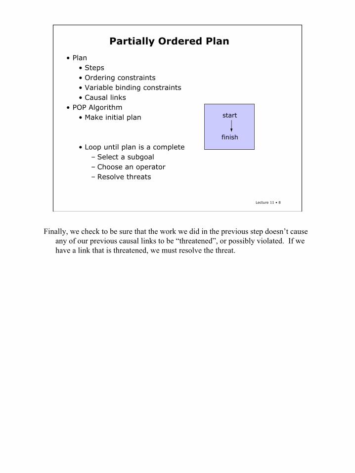
• Loop until plan is a complete– Select a subgoal– Choose an operator– Resolve threats
start
finish
Finally, we check to be sure that the work we did in the previous step doesn’t cause any of our previous causal links to be “threatened”, or possibly violated. If we have a link that is threatened, we must resolve the threat.

9
Lecture 11 • 9
Choose Operator
• Choose operator(c, Sneeds)
Okay. In the previous step, we chose a condition c that was an unsatisfied precondition of some step. Let’s call the step that needs c to be true “S sub needs”. Now, we need to find a way to make c true. There are two basic ways to do it: either we find some step in the existing plan that has c as an effect, or we add a new step to the plan.
10
Lecture 11 • 10
Choose Operator
• Choose operator(c, Sneeds)
Nondeterministic choice
We’re going to describe the algorithm for choosing operators using a special kind of programming language feature called “nondeterministic choice”. It’s a very convenient and effective way to describe search algorithms without getting into the details. A few real programming languages have been built that have this feature, but most don’t. We use it to make our pseudocode short.
11
Lecture 11 • 11
Choose Operator
• Choose operator(c, Sneeds)
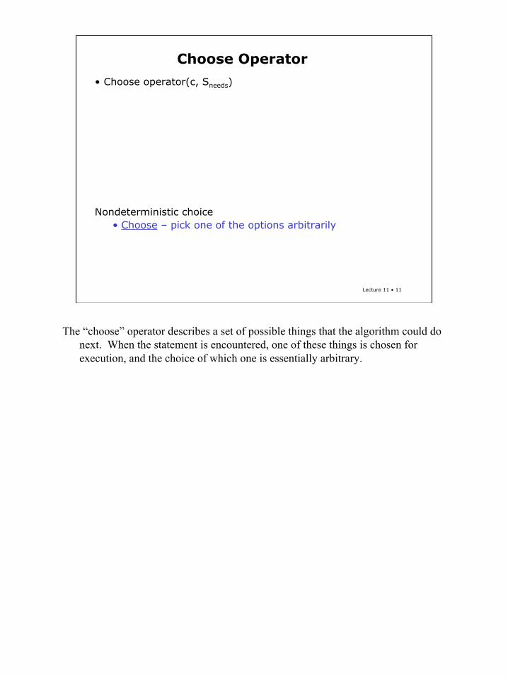
Nondeterministic choice• Choose – pick one of the options arbitrarily
The “choose” operator describes a set of possible things that the algorithm could do next. When the statement is encountered, one of these things is chosen for execution, and the choice of which one is essentially arbitrary.

12
Lecture 11 • 12
Choose Operator
• Choose operator(c, Sneeds)
Nondeterministic choice• Choose – pick one of the options arbitrarily• Fail – go back to most recent non-deterministic choice and
try a different one that has not been tried before
The “fail” operator says the algorithm should go back to the most recent non-deterministic choice point and choose a different option, from among those that have not yet been tried. If they’ve all been tried, then the whole “choose” operation fails, and we go back to the next most recent choose operation, and so on.
13
Lecture 11 • 13
Choose Operator
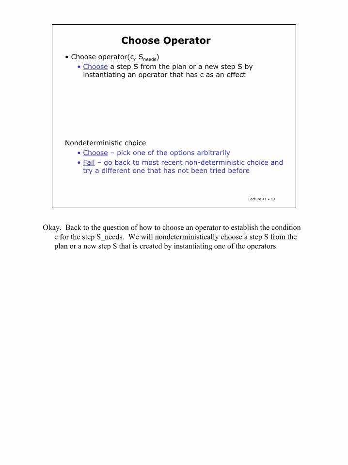
• Choose operator(c, Sneeds)• Choose a step S from the plan or a new step S by
instantiating an operator that has c as an effect
Nondeterministic choice• Choose – pick one of the options arbitrarily• Fail – go back to most recent non-deterministic choice and
try a different one that has not been tried before
Okay. Back to the question of how to choose an operator to establish the condition c for the step S_needs. We will nondeterministically choose a step S from the plan or a new step S that is created by instantiating one of the operators.
14
Lecture 11 • 14
Choose Operator
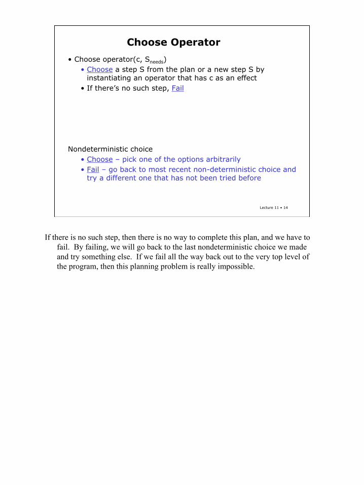
• Choose operator(c, Sneeds)• Choose a step S from the plan or a new step S by
instantiating an operator that has c as an effect• If there’s no such step, Fail
Nondeterministic choice• Choose – pick one of the options arbitrarily• Fail – go back to most recent non-deterministic choice and
try a different one that has not been tried before
If there is no such step, then there is no way to complete this plan, and we have to fail. By failing, we will go back to the last nondeterministic choice we made and try something else. If we fail all the way back out to the very top level of the program, then this planning problem is really impossible.
15
Lecture 11 • 15
Choose Operator
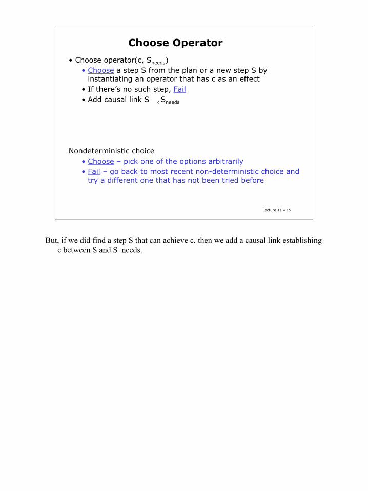
• Choose operator(c, Sneeds)• Choose a step S from the plan or a new step S by
instantiating an operator that has c as an effect• If there’s no such step, Fail• Add causal link S �c Sneeds
Nondeterministic choice• Choose – pick one of the options arbitrarily• Fail – go back to most recent non-deterministic choice and
try a different one that has not been tried before
But, if we did find a step S that can achieve c, then we add a causal link establishing c between S and S_needs.
16
Lecture 11 • 16
Choose Operator
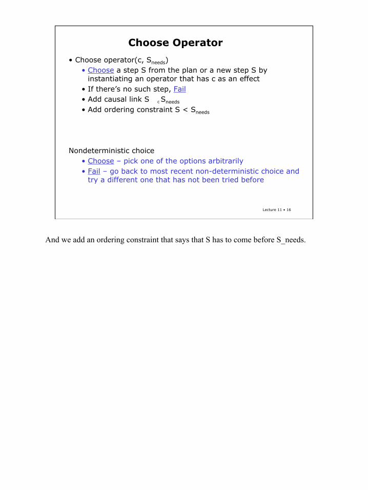
• Choose operator(c, Sneeds)• Choose a step S from the plan or a new step S by
instantiating an operator that has c as an effect• If there’s no such step, Fail• Add causal link S �c Sneeds
• Add ordering constraint S < Sneeds
Nondeterministic choice• Choose – pick one of the options arbitrarily• Fail – go back to most recent non-deterministic choice and
try a different one that has not been tried before
And we add an ordering constraint that says that S has to come before S_needs.
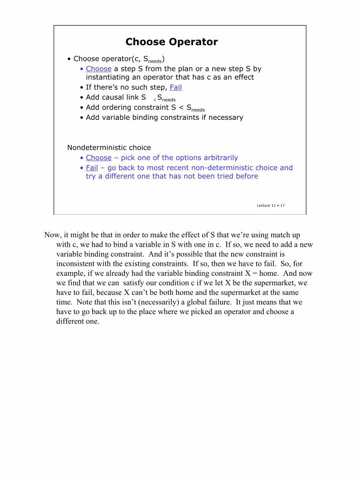
17
Lecture 11 • 17
Choose Operator
• Choose operator(c, Sneeds)• Choose a step S from the plan or a new step S by
instantiating an operator that has c as an effect• If there’s no such step, Fail• Add causal link S �c Sneeds
• Add ordering constraint S < Sneeds
• Add variable binding constraints if necessary
Nondeterministic choice• Choose – pick one of the options arbitrarily• Fail – go back to most recent non-deterministic choice and
try a different one that has not been tried before
Now, it might be that in order to make the effect of S that we’re using match up with c, we had to bind a variable in S with one in c. If so, we need to add a new variable binding constraint. And it’s possible that the new constraint is inconsistent with the existing constraints. If so, then we have to fail. So, for example, if we already had the variable binding constraint X = home. And now we find that we can satisfy our condition c if we let X be the supermarket, we have to fail, because X can’t be both home and the supermarket at the same time. Note that this isn’t (necessarily) a global failure. It just means that we have to go back up to the place where we picked an operator and choose a different one.

18
Lecture 11 • 18
Choose Operator
• Choose operator(c, Sneeds)• Choose a step S from the plan or a new step S by
instantiating an operator that has c as an effect• If there’s no such step, Fail• Add causal link S �c Sneeds
• Add ordering constraint S < Sneeds
• Add variable binding constraints if necessary• Add S to steps if necessary
Nondeterministic choice• Choose – pick one of the options arbitrarily• Fail – go back to most recent non-deterministic choice and
try a different one that has not been tried before
Finally, if S was a new step, we add it to the steps of the plan.
19
Lecture 11 • 19
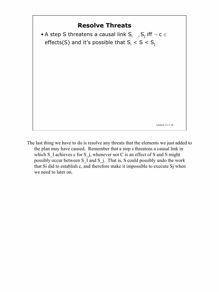
Resolve Threats• A step S threatens a causal link Si �c Sj iff ¬ c ∈
effects(S) and it’s possible that Si < S < Sj
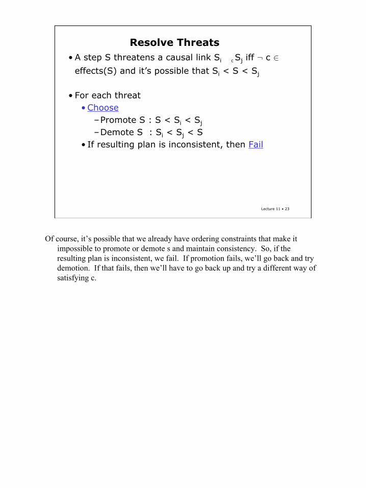
The last thing we have to do is resolve any threats that the elements we just added to the plan may have caused. Remember that a step s threatens a causal link in which S_I achieves c for S_j, whenever not C is an effect of S and S might possibly occur between S_I and S_j. That is, S could possibly undo the work that Si did to establish c, and therefore make it impossible to execute Sj when we need to later on.
20
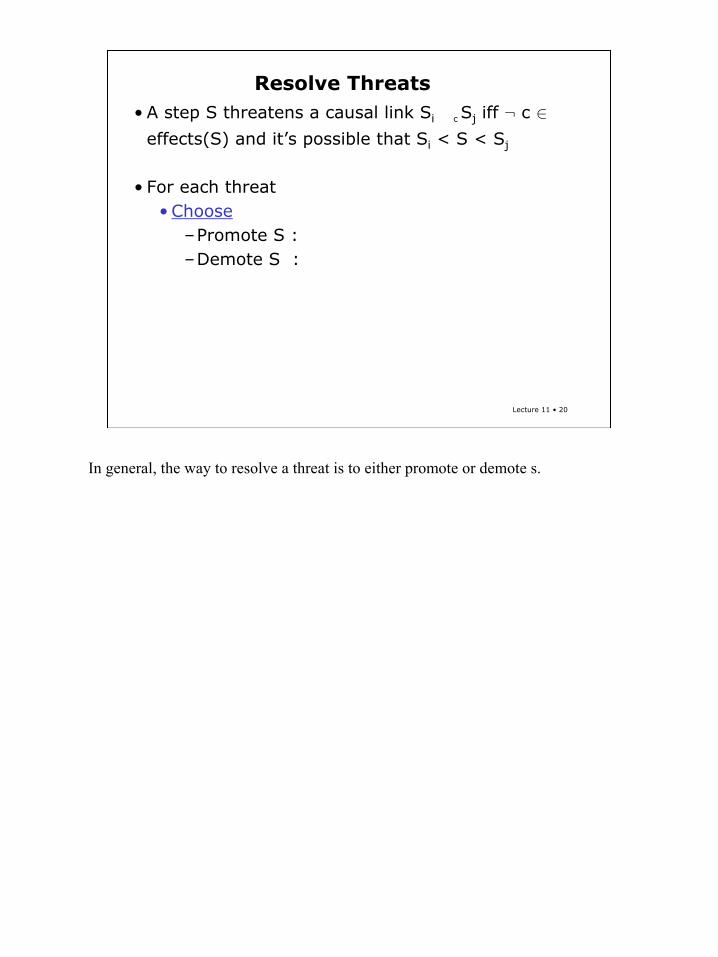
Lecture 11 • 20
Resolve Threats• A step S threatens a causal link Si �c Sj iff ¬ c ∈
effects(S) and it’s possible that Si < S < Sj
• For each threat• Choose
–Promote S :–Demote S :
In general, the way to resolve a threat is to either promote or demote s.

21
Lecture 11 • 21
Resolve Threats• A step S threatens a causal link Si �c Sj iff ¬ c ∈
effects(S) and it’s possible that Si < S < Sj
• For each threat• Choose
–Promote S : S < Si < Sj
–Demote S :
Promoting s means requiring that it come before both Si and Sj. Then, even if it does make c false, it’s not a problem, because Si will make it true again.
22
Lecture 11 • 22
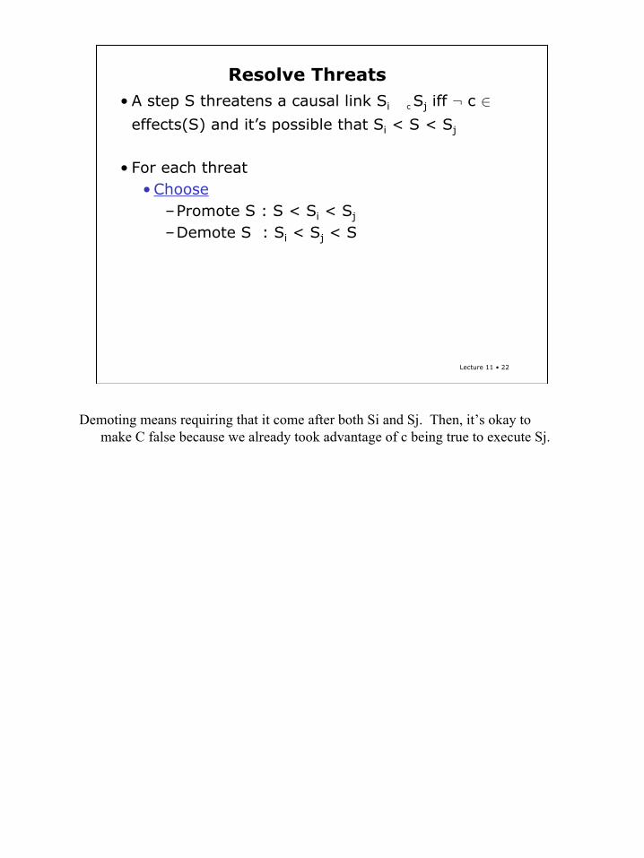
Resolve Threats• A step S threatens a causal link Si �c Sj iff ¬ c ∈
effects(S) and it’s possible that Si < S < Sj
• For each threat• Choose
–Promote S : S < Si < Sj
–Demote S : Si < Sj < S
Demoting means requiring that it come after both Si and Sj. Then, it’s okay to make C false because we already took advantage of c being true to execute Sj.
23
Lecture 11 • 23
Resolve Threats• A step S threatens a causal link Si �c Sj iff ¬ c ∈
effects(S) and it’s possible that Si < S < Sj
• For each threat• Choose
–Promote S : S < Si < Sj
–Demote S : Si < Sj < S• If resulting plan is inconsistent, then Fail
Of course, it’s possible that we already have ordering constraints that make it impossible to promote or demote s and maintain consistency. So, if the resulting plan is inconsistent, we fail. If promotion fails, we’ll go back and try demotion. If that fails, then we’ll have to go back up and try a different way of satisfying c.

24
Lecture 11 • 24
Threats with Variables
If c has variables in it, things are kind of tricky.• S is a threat if there is any instantiation of the
variables that makes ¬ c ∈ effects(S)
If the condition c has a variable in it, then things get a bit more tricky. Now we’ll say that S is a threat not just if not C is in the effects of S, but if there is any instantiations of the variables of C or S that would cause not C to be in the effects of S.

25
Lecture 11 • 25
Threats with Variables
If c has variables in it, things are kind of tricky.• S is a threat if there is any instantiation of the
variables that makes ¬ c ∈ effects(S)
• We could possibly resolve the threat by adding a negative variable binding constraint, saying that two variables or a variable and a constant cannot be bound to one another
If we have a threat with variables, then there is one more potential way to resolve the threat. We could constraint the variables not to be bound in a way that lets C match up with a negative effect in S.

26
Lecture 11 • 26
Threats with Variables
If c has variables in it, things are kind of tricky.• S is a threat if there is any instantiation of the
variables that makes ¬ c ∈ effects(S)
• We could possibly resolve the threat by adding a negative variable binding constraint, saying that two variables or a variable and a constant cannot be bound to one another
• Another strategy is to ignore such threats until the very end, hoping that the variables will become bound and make things easier to deal with
Another strategy is to ignore such threats until the very end, hoping that the variables will become bound and make things easier to deal with.
27
Lecture 11 • 27
Shopping Domain
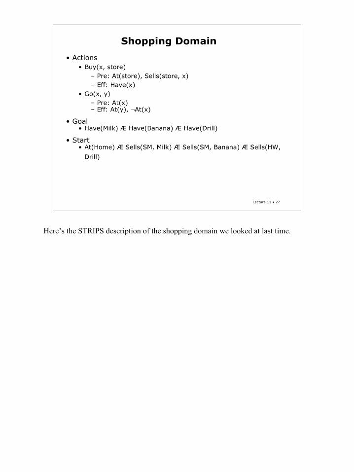
• Actions• Buy(x, store)
– Pre: At(store), Sells(store, x)– Eff: Have(x)
• Go(x, y)– Pre: At(x)– Eff: At(y), ¬At(x)
• Goal• Have(Milk) Æ Have(Banana) Æ Have(Drill)
• Start• At(Home) Æ Sells(SM, Milk) Æ Sells(SM, Banana) Æ Sells(HW,
Drill)
Here’s the STRIPS description of the shopping domain we looked at last time.
28
Lecture 11 • 28
Shop ‘til You Drop!
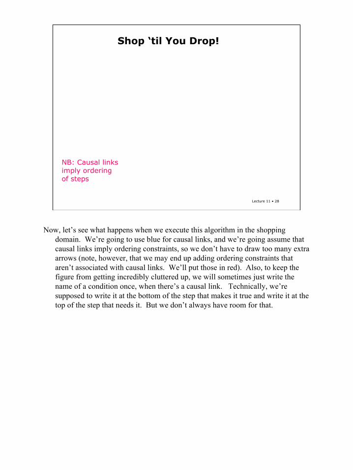
NB: Causal links imply ordering of steps
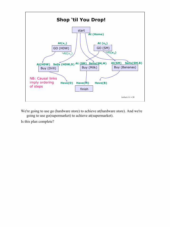
Now, let’s see what happens when we execute this algorithm in the shopping domain. We’re going to use blue for causal links, and we’re going assume that causal links imply ordering constraints, so we don’t have to draw too many extra arrows (note, however, that we may end up adding ordering constraints that aren’t associated with causal links. We’ll put those in red). Also, to keep the figure from getting incredibly cluttered up, we will sometimes just write the name of a condition once, when there’s a causal link. Technically, we’re supposed to write it at the bottom of the step that makes it true and write it at the top of the step that needs it. But we don’t always have room for that.
29
Lecture 11 • 29
Shop ‘til You Drop!
startAt (Home)
Buy (Bananas)Buy (Drill)Sells (HDW,D)At(HDW)
Buy (Milk)At (SM) Sells(SM,M)
finish
Have(D) Have(B)Have(M)
At(SM) Sells(SM,B)
NB: Causal links imply ordering of steps
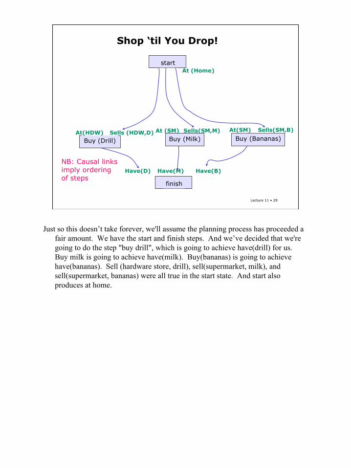
Just so this doesn’t take forever, we'll assume the planning process has proceeded a fair amount. We have the start and finish steps. And we’ve decided that we're going to do the step "buy drill", which is going to achieve have(drill) for us. Buy milk is going to achieve have(milk). Buy(bananas) is going to achieve have(bananas). Sell (hardware store, drill), sell(supermarket, milk), and sell(supermarket, bananas) were all true in the start state. And start also produces at home.
30
Lecture 11 • 30
Shop ‘til You Drop!
¬At(x2)
GO (SM)
At (x2)
GO (HDW)
At(x1)
¬At(x1)
startAt (Home)
Buy (Bananas)Buy (Drill)Sells (HDW,D)At(HDW)
Buy (Milk)At (SM) Sells(SM,M)
finish
Have(D) Have(B)Have(M)
At(SM) Sells(SM,B)
NB: Causal links imply ordering of steps
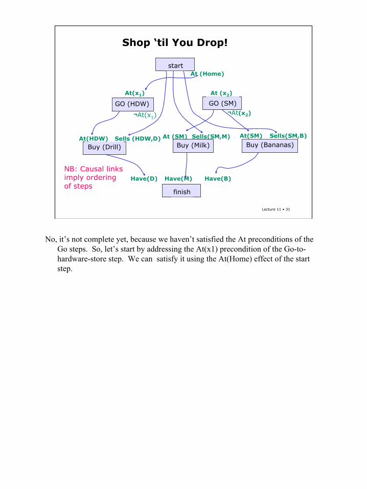
We're going to use go (hardware store) to achieve at(hardware store). And we're going to use go(supermarket) to achieve at(supermarket).
Is this plan complete?
31
Lecture 11 • 31
Shop ‘til You Drop!
¬At(x2)
GO (SM)
At (x2)
GO (HDW)
At(x1)
¬At(x1)
startAt (Home)
Buy (Bananas)Buy (Drill)Sells (HDW,D)At(HDW)
Buy (Milk)At (SM) Sells(SM,M)
finish
Have(D) Have(B)Have(M)
At(SM) Sells(SM,B)
NB: Causal links imply ordering of steps
No, it’s not complete yet, because we haven’t satisfied the At preconditions of the Go steps. So, let’s start by addressing the At(x1) precondition of the Go-to-hardware-store step. We can satisfy it using the At(Home) effect of the start step.
32
Lecture 11 • 32
Shop ‘til You Drop!
¬At(x2)
GO (SM)
At (x2)
GO (HDW)
At(x1)
¬At(x1)
startAt (Home)
Buy (Bananas)Buy (Drill)Sells (HDW,D)At(HDW)
Buy (Milk)At (SM) Sells(SM,M)
finish
Have(D) Have(B)Have(M)
At(SM) Sells(SM,B)
x1=Home
NB: Causal links imply ordering of steps
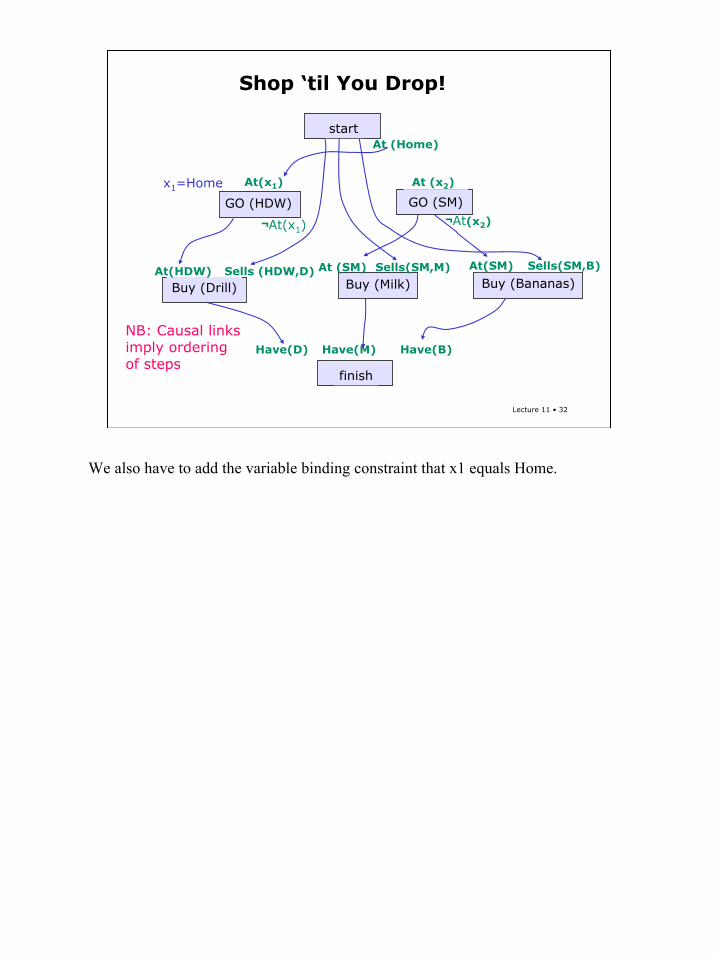
We also have to add the variable binding constraint that x1 equals Home.
33
Lecture 11 • 33
Shop ‘til You Drop!
¬At(x2)
GO (SM)
At (x2)
GO (HDW)
At(x1)
¬At(x1)
startAt (Home)
Buy (Bananas)Buy (Drill)Sells (HDW,D)At(HDW)
Buy (Milk)At (SM) Sells(SM,M)
finish
Have(D) Have(B)Have(M)
At(SM) Sells(SM,B)
x1=Home
NB: Causal links imply ordering of steps
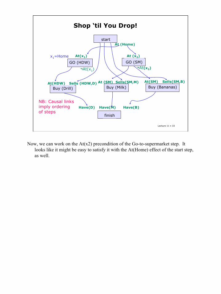
Now, we can work on the At(x2) precondition of the Go-to-supermarket step. It looks like it might be easy to satisfy it with the At(Home) effect of the start step, as well.
34
Lecture 11 • 34
Shop ‘til You Drop!
¬At(x2)
GO (SM)
At (x2)
GO (HDW)
At(x1)
¬At(x1)
startAt (Home)
Buy (Bananas)Buy (Drill)Sells (HDW,D)At(HDW)
Buy (Milk)At (SM) Sells(SM,M)
finish
Have(D) Have(B)Have(M)
At(SM) Sells(SM,B)
x1=Home x2=Home
NB: Causal links imply ordering of steps
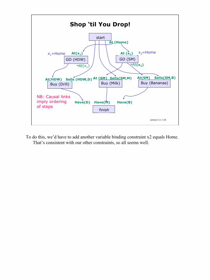
To do this, we’d have to add another variable binding constraint x2 equals Home. That’s consistent with our other constraints, so all seems well.
35
Lecture 11 • 35
Shop ‘til You Drop!
¬At(x2)
GO (SM)
At (x2)
GO (HDW)
At(x1)
¬At(x1)
startAt (Home)
Buy (Bananas)Buy (Drill)Sells (HDW,D)At(HDW)
Buy (Milk)At (SM) Sells(SM,M)
finish
Have(D) Have(B)Have(M)
At(SM) Sells(SM,B)
x1=Home x2=Home
NB: Causal links imply ordering of steps
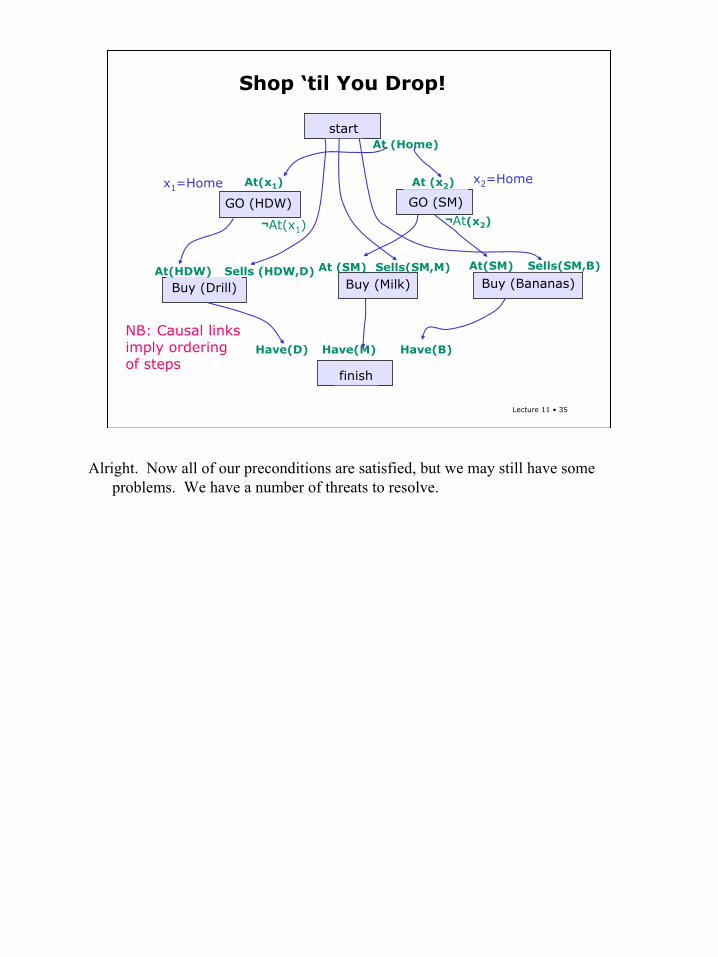
Alright. Now all of our preconditions are satisfied, but we may still have some problems. We have a number of threats to resolve.
36
Lecture 11 • 36
Shop ‘til You Drop!
¬At(x2)
GO (SM)
At (x2)
GO (HDW)
At(x1)
¬At(x1)
startAt (Home)
Buy (Bananas)Buy (Drill)Sells (HDW,D)At(HDW)
Buy (Milk)At (SM) Sells(SM,M)
finish
Have(D) Have(B)Have(M)
At(SM) Sells(SM,B)
x1=Home x2=Home
NB: Causal links imply ordering of steps
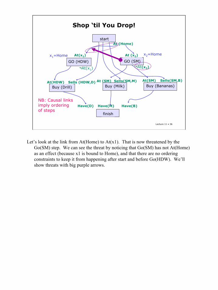
Let’s look at the link from At(Home) to At(x1). That is now threatened by the Go(SM) step. We can see the threat by noticing that Go(SM) has not At(Home) as an effect (because x1 is bound to Home), and that there are no ordering constraints to keep it from happening after start and before Go(HDW). We’ll show threats with big purple arrows.
37
Lecture 11 • 37
Shop ‘til You Drop!
¬At(x2)
GO (SM)
At (x2)
GO (HDW)
At(x1)
¬At(x1)
startAt (Home)
Buy (Bananas)Buy (Drill)Sells (HDW,D)At(HDW)
Buy (Milk)At (SM) Sells(SM,M)
finish
Have(D) Have(B)Have(M)
At(SM) Sells(SM,B)
x1=Home x2=Home
NB: Causal links imply ordering of steps
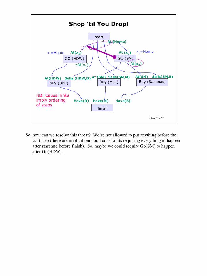
So, how can we resolve this threat? We’re not allowed to put anything before the start step (there are implicit temporal constraints requiring everything to happen after start and before finish). So, maybe we could require Go(SM) to happen after Go(HDW).
38
Lecture 11 • 38
Shop ‘til You Drop!
¬At(x2)
GO (SM)
At (x2)
GO (HDW)
At(x1)
¬At(x1)
startAt (Home)
Buy (Bananas)Buy (Drill)Sells (HDW,D)At(HDW)
Buy (Milk)At (SM) Sells(SM,M)
finish
Have(D) Have(B)Have(M)
At(SM) Sells(SM,B)
x1=Home x2=Home
NB: Causal links imply ordering of steps
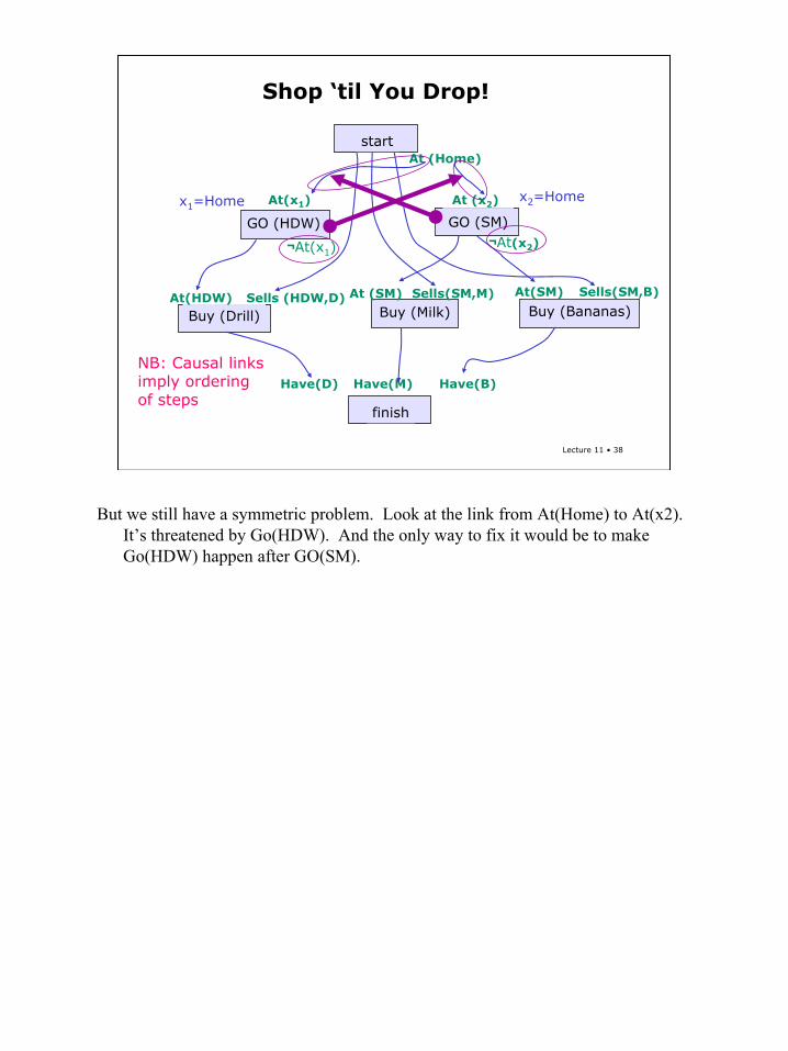
But we still have a symmetric problem. Look at the link from At(Home) to At(x2). It’s threatened by Go(HDW). And the only way to fix it would be to make Go(HDW) happen after GO(SM).
39
Lecture 11 • 39
Shop ‘til You Drop!
startAt (Home)
Buy (Bananas)Buy (Drill)Sells (HDW,D)At(HDW)
¬At(x2)
GO (SM)At (x2)
Buy (Milk)At (SM) Sells(SM,M)
finish
Have(D) Have(B)Have(M)
At(SM) Sells(SM,B)
GO (HDW)
At(x1)
¬At(x1)
x1=Home x2=Home
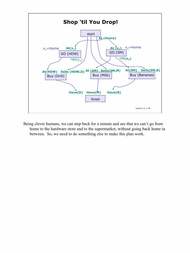
Being clever humans, we can step back for a minute and see that we can’t go from home to the hardware store and to the supermarket, without going back home in between. So, we need to do something else to make this plan work.
40
Lecture 11 • 40
Shop ‘til You Drop!
startAt (Home)
Buy (Bananas)Buy (Drill)Sells (HDW,D)At(HDW)
¬At(x2)
GO (SM)At (x2)
Buy (Milk)At (SM) Sells(SM,M)
finish
Have(D) Have(B)Have(M)
At(SM) Sells(SM,B)
GO (HDW)
At(x1)
¬At(x1)
x1=Home x2=Home
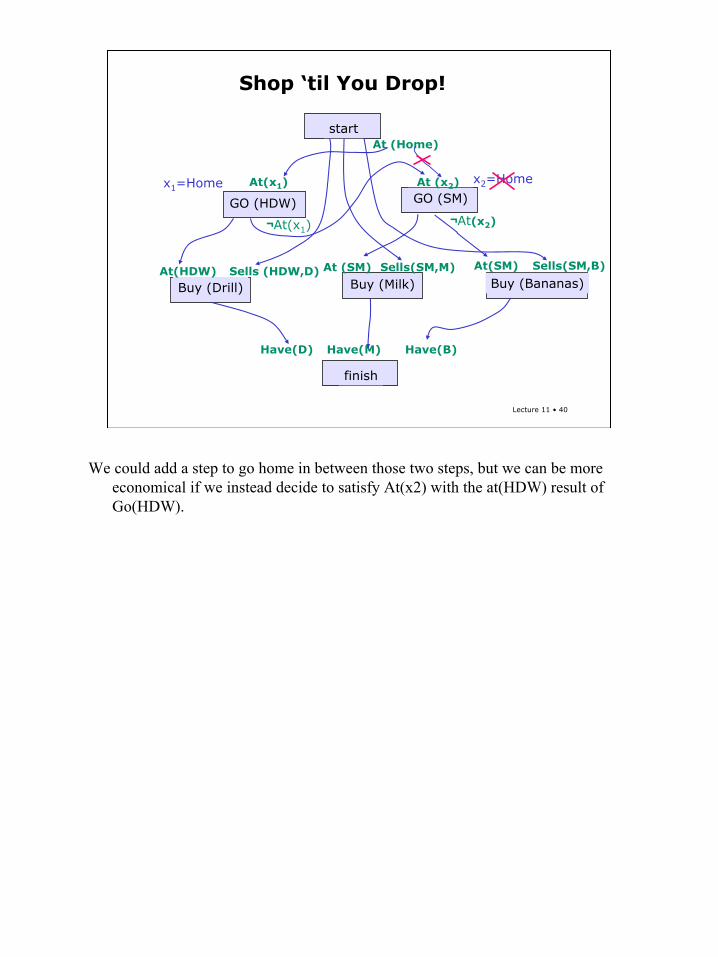
We could add a step to go home in between those two steps, but we can be more economical if we instead decide to satisfy At(x2) with the at(HDW) result of Go(HDW).
41
Lecture 11 • 41
Shop ‘til You Drop!
startAt (Home)
Buy (Bananas)Buy (Drill)Sells (HDW,D)At(HDW)
¬At(x2)
GO (SM)At (x2)
Buy (Milk)At (SM) Sells(SM,M)
finish
Have(D) Have(B)Have(M)
At(SM) Sells(SM,B)
GO (HDW)
At(x1)
¬At(x1)
x1=Home x2=Home
x2=HDW
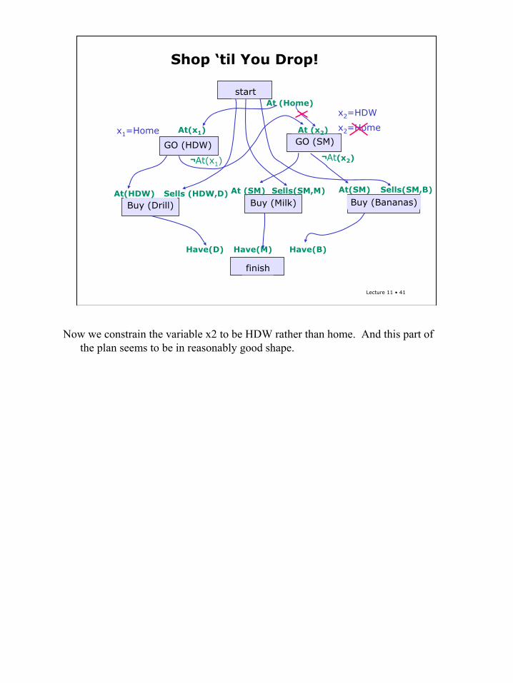
Now we constrain the variable x2 to be HDW rather than home. And this part of the plan seems to be in reasonably good shape.
42
Lecture 11 • 42
Shop ‘til You Drop!
startAt (Home)
Buy (Bananas)Buy (Drill)Sells (HDW,D)At(HDW)
¬At(x2)
GO (SM)At (x2)
Buy (Milk)At (SM) Sells(SM,M)
finish
Have(D) Have(B)Have(M)
At(SM) Sells(SM,B)
GO (HDW)
At(x1)
¬At(x1)
x1=Home x2=Home
x2=HDW
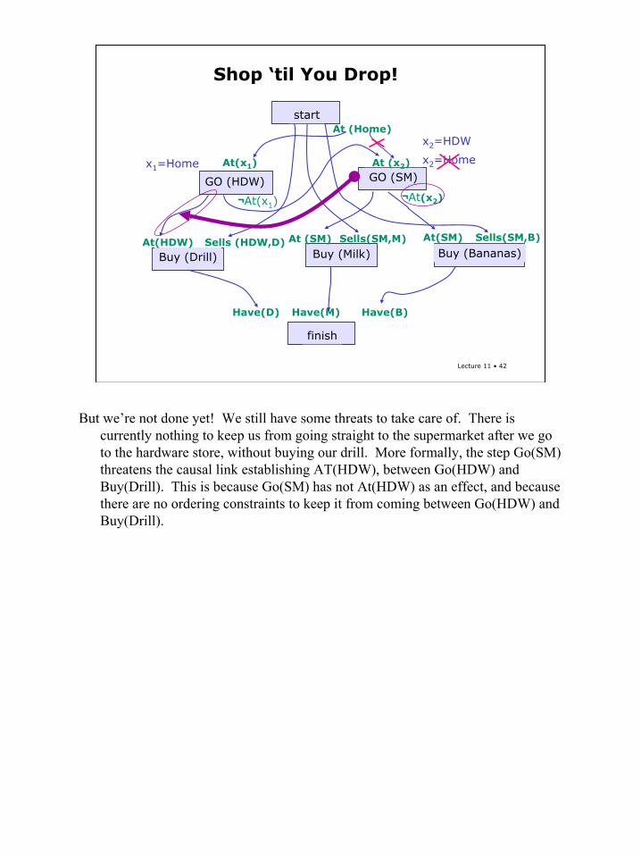
But we’re not done yet! We still have some threats to take care of. There is currently nothing to keep us from going straight to the supermarket after we go to the hardware store, without buying our drill. More formally, the step Go(SM) threatens the causal link establishing AT(HDW), between Go(HDW) and Buy(Drill). This is because Go(SM) has not At(HDW) as an effect, and because there are no ordering constraints to keep it from coming between Go(HDW) and Buy(Drill).
43
Lecture 11 • 43
Shop ‘til You Drop!
startAt (Home)
Buy (Bananas)Buy (Drill)Sells (HDW,D)At(HDW)
¬At(x2)
GO (SM)At (x2)
Buy (Milk)At (SM) Sells(SM,M)
finish
Have(D) Have(B)Have(M)
At(SM) Sells(SM,B)
GO (HDW)
At(x1)
¬At(x1)
x1=Home x2=Home
x2=HDW
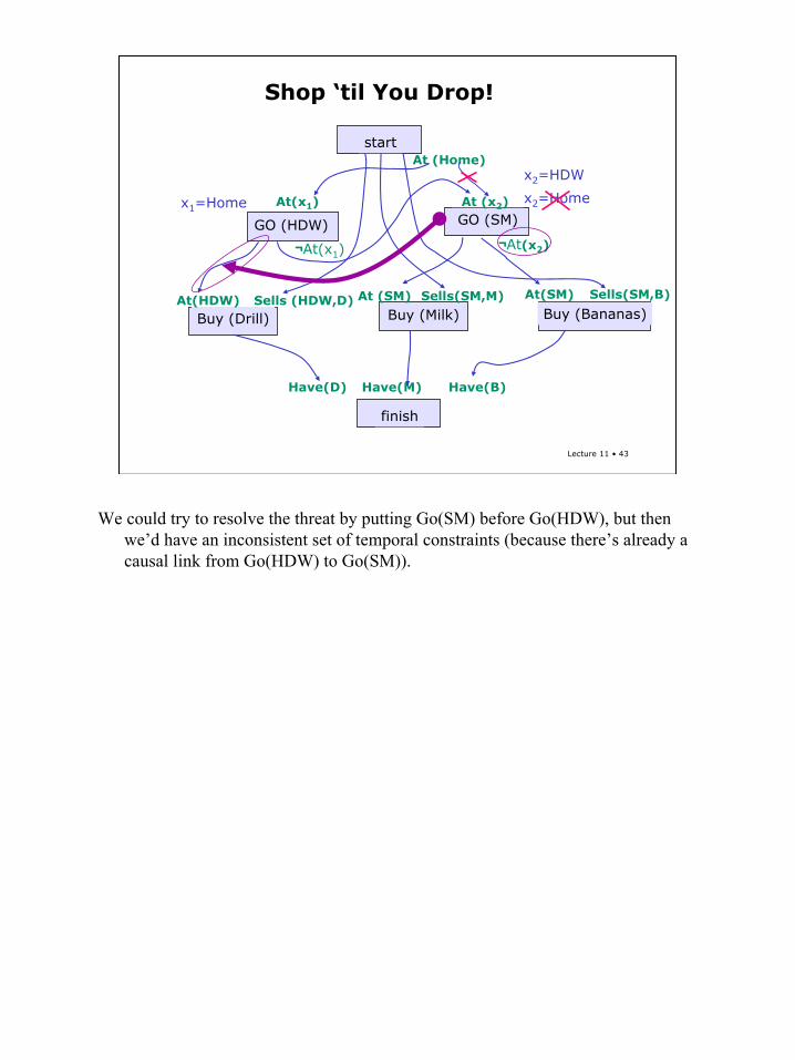
We could try to resolve the threat by putting Go(SM) before Go(HDW), but then we’d have an inconsistent set of temporal constraints (because there’s already a causal link from Go(HDW) to Go(SM)).
44
Lecture 11 • 44
Shop ‘til You Drop!
startAt (Home)
Buy (Bananas)Buy (Drill)Sells (HDW,D)At(HDW)
¬At(x2)
GO (SM)At (x2)
Buy (Milk)At (SM) Sells(SM,M)
finish
Have(D) Have(B)Have(M)
At(SM) Sells(SM,B)
GO (HDW)
At(x1)
¬At(x1)
x1=Home x2=Home
x2=HDW
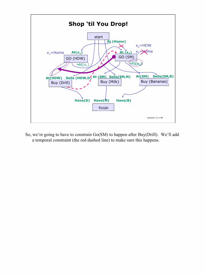
So, we’re going to have to constrain Go(SM) to happen after Buy(Drill). We’ll add a temporal constraint (the red dashed line) to make sure this happens.
45
Lecture 11 • 45
Shop ‘til You Drop!
startAt (Home)
Buy (Bananas)Buy (Drill)Sells (HDW,D)At(HDW)
¬At(x2)
GO (SM)At (x2)
Buy (Milk)At (SM) Sells(SM,M)
finish
Have(D) Have(B)Have(M)
At(SM) Sells(SM,B)
GO (HDW)
At(x1)
¬At(x1)
x1=Home x2=Home
x2=HDW
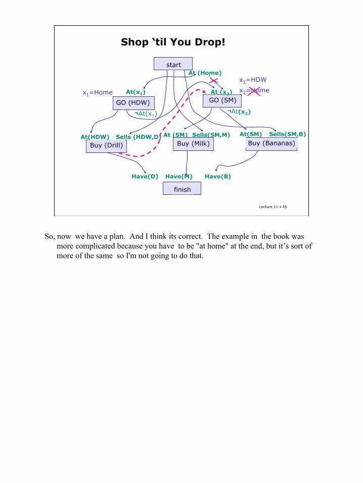
So, now we have a plan. And I think its correct. The example in the book was more complicated because you have to be "at home" at the end, but it’s sort of more of the same so I'm not going to do that.
46
Lecture 11 • 46
Shop ‘til You Drop!
startAt (Home)
Buy (Bananas)Buy (Drill)Sells (HDW,D)At(HDW)
¬At(x2)
GO (SM)At (x2)
Buy (Milk)At (SM) Sells(SM,M)
finish
Have(D) Have(B)Have(M)
At(SM) Sells(SM,B)
GO (HDW)
At(x1)
¬At(x1)
x1=Home x2=Home
x2=HDW
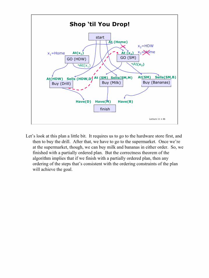
Let’s look at this plan a little bit. It requires us to go to the hardware store first, and then to buy the drill. After that, we have to go to the supermarket. Once we’re at the supermarket, though, we can buy milk and bananas in either order. So, we finished with a partially ordered plan. But the correctness theorem of the algorithm implies that if we finish with a partially ordered plan, then any ordering of the steps that’s consistent with the ordering constraints of the plan will achieve the goal.
47
Lecture 11 • 47
Shop ‘til You Drop!
startAt (Home)
Buy (Bananas)Buy (Drill)Sells (HDW,D)At(HDW)
¬At(x2)
GO (SM)At (x2)
Buy (Milk)At (SM) Sells(SM,M)
finish
Have(D) Have(B)Have(M)
At(SM) Sells(SM,B)
GO (HDW)
At(x1)
¬At(x1)
x1=Home x2=Home
x2=HDW
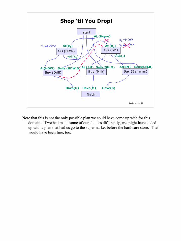
Note that this is not the only possible plan we could have come up with for this domain. If we had made some of our choices differently, we might have ended up with a plan that had us go to the supermarket before the hardware store. That would have been fine, too.
48
Lecture 11 • 48
Shop ‘til You Drop!
startAt (Home)
Buy (Bananas)Buy (Drill)Sells (HDW,D)At(HDW)
¬At(x2)
GO (SM)At (x2)
Buy (Milk)At (SM) Sells(SM,M)
finish
Have(D) Have(B)Have(M)
At(SM) Sells(SM,B)
GO (HDW)
At(x1)
¬At(x1)
x1=Home x2=Home
x2=HDW
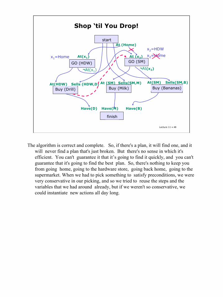
The algorithm is correct and complete. So, if there's a plan, it will find one, and it will never find a plan that's just broken. But there's no sense in which it's efficient. You can't guarantee it that it’s going to find it quickly, and you can't guarantee that it's going to find the best plan. So, there's nothing to keep you from going home, going to the hardware store, going back home, going to the supermarket. When we had to pick something to satisfy preconditions, we were very conservative in our picking, and so we tried to reuse the steps and the variables that we had around already, but if we weren't so conservative, we could instantiate new actions all day long.
49
Lecture 11 • 49
Shop ‘til You Drop!
startAt (Home)
Buy (Bananas)Buy (Drill)Sells (HDW,D)At(HDW)
¬At(x2)
GO (SM)At (x2)
Buy (Milk)At (SM) Sells(SM,M)
finish
Have(D) Have(B)Have(M)
At(SM) Sells(SM,B)
GO (HDW)
At(x1)
¬At(x1)
x1=Home x2=Home
x2=HDW
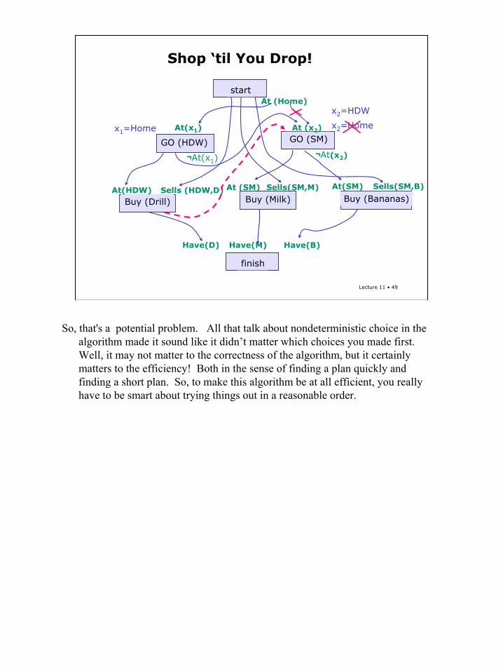
So, that's a potential problem. All that talk about nondeterministic choice in the algorithm made it sound like it didn’t matter which choices you made first. Well, it may not matter to the correctness of the algorithm, but it certainly matters to the efficiency! Both in the sense of finding a plan quickly and finding a short plan. So, to make this algorithm be at all efficient, you really have to be smart about trying things out in a reasonable order.
50
Lecture 11 • 50
Shop ‘til You Drop!
startAt (Home)
Buy (Bananas)Buy (Drill)Sells (HDW,D)At(HDW)
¬At(x2)
GO (SM)At (x2)
Buy (Milk)At (SM) Sells(SM,M)
finish
Have(D) Have(B)Have(M)
At(SM) Sells(SM,B)
GO (HDW)
At(x1)
¬At(x1)
x1=Home x2=Home
x2=HDW
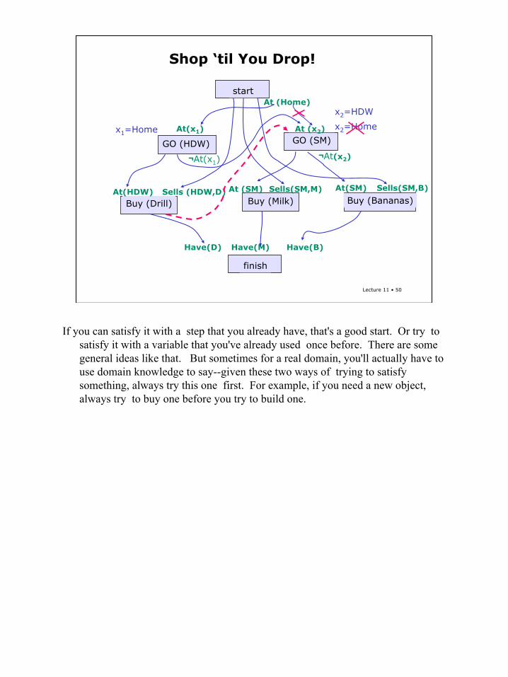
If you can satisfy it with a step that you already have, that's a good start. Or try to satisfy it with a variable that you've already used once before. There are some general ideas like that. But sometimes for a real domain, you'll actually have to use domain knowledge to say--given these two ways of trying to satisfy something, always try this one first. For example, if you need a new object, always try to buy one before you try to build one.
51
Lecture 11 • 51
Subgoal Dependence
C
A B
Goal: on(A,B) Æ on(B,C)
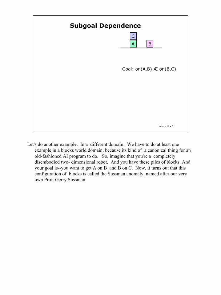
Let's do another example. In a different domain. We have to do at least one example in a blocks world domain, because its kind of a canonical thing for an old-fashioned AI program to do. So, imagine that you're a completely disembodied two- dimensional robot. And you have these piles of blocks. And your goal is--you want to get A on B and B on C. Now, it turns out that thisconfiguration of blocks is called the Sussman anomaly, named after our very own Prof. Gerry Sussman.
52
Lecture 11 • 52
Subgoal Dependence
C
A B
Goal: on(A,B) Æ on(B,C)
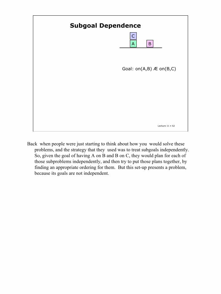
Back when people were just starting to think about how you would solve these problems, and the strategy that they used was to treat subgoals independently. So, given the goal of having A on B and B on C, they would plan for each of those subproblems independently, and then try to put those plans together, by finding an appropriate ordering for them. But this set-up presents a problem, because its goals are not independent.
53
Lecture 11 • 53
Subgoal Dependence
C
A B
Goal: on(A,B) Æ on(B,C)
C
A
B
Put A on B first
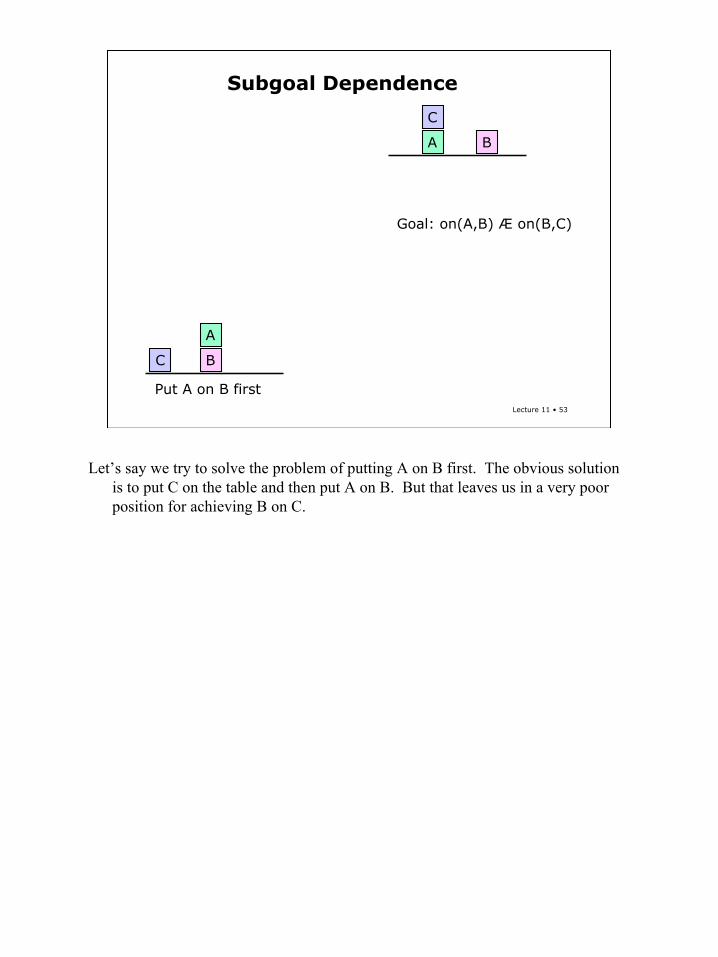
Let’s say we try to solve the problem of putting A on B first. The obvious solution is to put C on the table and then put A on B. But that leaves us in a very poor position for achieving B on C.
54
Lecture 11 • 54
Subgoal Dependence
C
A B
Goal: on(A,B) Æ on(B,C)
C
A
B
C
A
B
Put A on B first Put B on C first
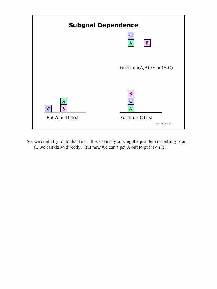
So, we could try to do that first. If we start by solving the problem of putting B on C, we can do so directly. But now we can’t get A out to put it on B!
55
Lecture 11 • 55
Subgoal Dependence
C
A B
Goal: on(A,B) Æ on(B,C)
C
A
B
C
A
B
Put A on B first Put B on C first
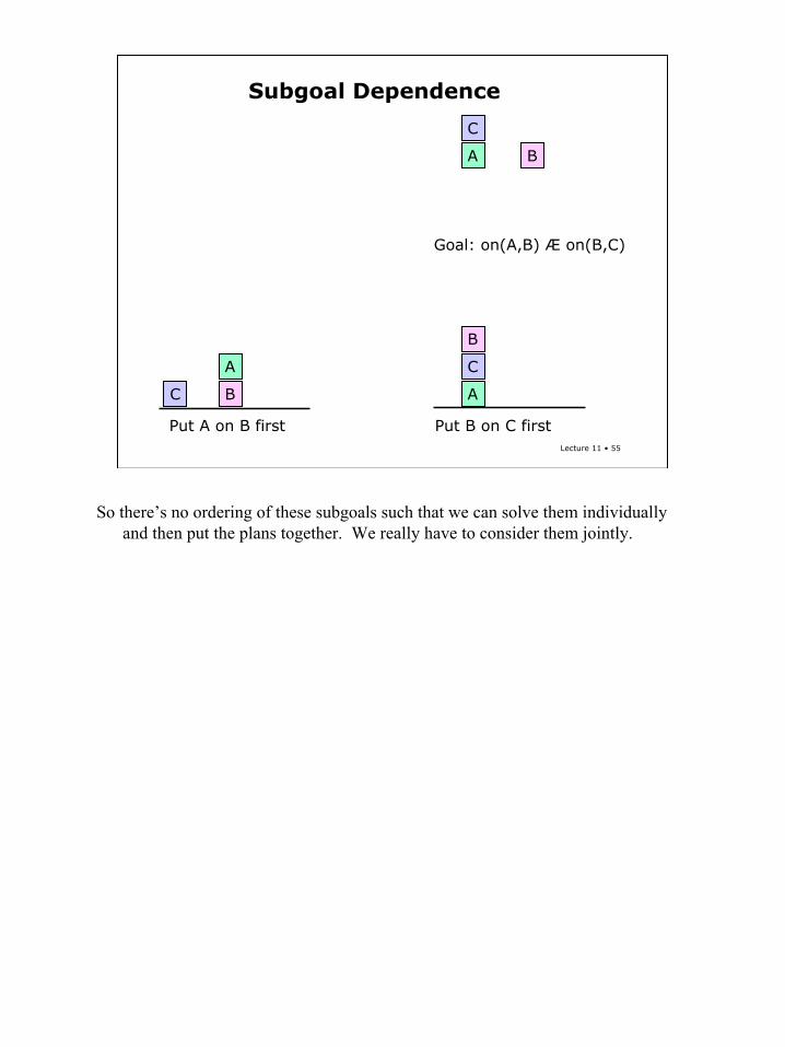
So there’s no ordering of these subgoals such that we can solve them individually and then put the plans together. We really have to consider them jointly.
56
Lecture 11 • 56
Subgoal Dependence
C
A B
Objects: A, B, C, Tableon(x,y)clear(x)Goal: on(A,B) Æ on(B,C)
C
A
B
C
A
B
Put A on B first Put B on C first
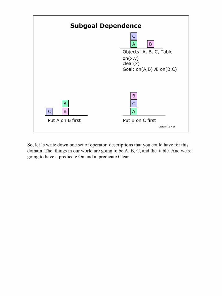
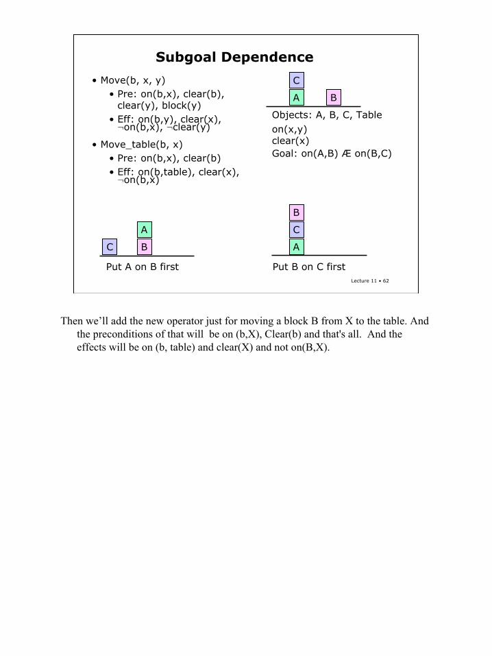
So, let ‘s write down one set of operator descriptions that you could have for this domain. The things in our world are going to be A, B, C, and the table. And we're going to have a predicate On and a predicate Clear
57
Lecture 11 • 57
Subgoal Dependence
• Move(b, x, y)• Pre: on(b,x), clear(b),
clear(y)• Eff: on(b,y), clear(x), ¬on(b,x), ¬clear(y)
C
A B
Objects: A, B, C, Tableon(x,y)clear(x)Goal: on(A,B) Æ on(B,C)
C
A
B
C
A
B
Put A on B first Put B on C first
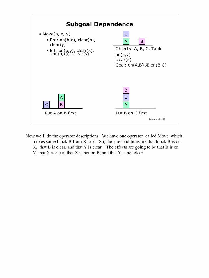
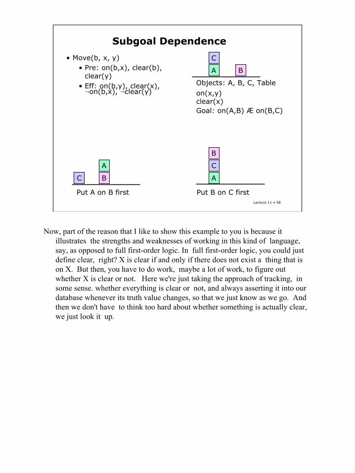
Now we’ll do the operator descriptions. We have one operator called Move, which moves some block B from X to Y. So, the preconditions are that block B is on X, that B is clear, and that Y is clear. The effects are going to be that B is on Y, that X is clear, that X is not on B, and that Y is not clear.
58
Lecture 11 • 58
Subgoal Dependence
• Move(b, x, y)• Pre: on(b,x), clear(b),
clear(y)• Eff: on(b,y), clear(x), ¬on(b,x), ¬clear(y)
C
A B
Objects: A, B, C, Tableon(x,y)clear(x)Goal: on(A,B) Æ on(B,C)
C
A
B
C
A
B
Put A on B first Put B on C first
Now, part of the reason that I like to show this example to you is because it illustrates the strengths and weaknesses of working in this kind of language, say, as opposed to full first-order logic. In full first-order logic, you could just define clear, right? X is clear if and only if there does not exist a thing that is on X. But then, you have to do work, maybe a lot of work, to figure out whether X is clear or not. Here we're just taking the approach of tracking, in some sense. whether everything is clear or not, and always asserting it into our database whenever its truth value changes, so that we just know as we go. And then we don't have to think too hard about whether something is actually clear, we just look it up.
59
Lecture 11 • 59
Subgoal Dependence
• Move(b, x, y)• Pre: on(b,x), clear(b),
clear(y)• Eff: on(b,y), clear(x), ¬on(b,x), ¬clear(y)
C
A B
Objects: A, B, C, Tableon(x,y)clear(x)Goal: on(A,B) Æ on(B,C)
C
A
B
C
A
B
Put A on B first Put B on C first
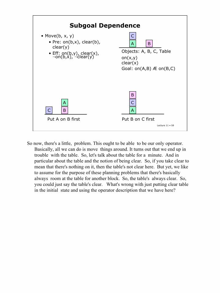
So now, there's a little, problem. This ought to be able to be our only operator. Basically, all we can do is move things around. It turns out that we end up in trouble with the table. So, let's talk about the table for a minute. And in particular about the table and the notion of being clear. So, if you take clear to mean that there's nothing on it, then the table's not clear here. But yet, we like to assume for the purpose of these planning problems that there's basically always room at the table for another block. So, the table's always clear. So, you could just say the table's clear. What's wrong with just putting clear table in the initial state and using the operator description that we have here?
60
Lecture 11 • 60
Subgoal Dependence
• Move(b, x, y)• Pre: on(b,x), clear(b),
clear(y)• Eff: on(b,y), clear(x), ¬on(b,x), ¬clear(y)
• Move_table(b, x)
C
A B
Objects: A, B, C, Tableon(x,y)clear(x)Goal: on(A,B) Æ on(B,C)
C
A
B
C
A
B
Put A on B first Put B on C first
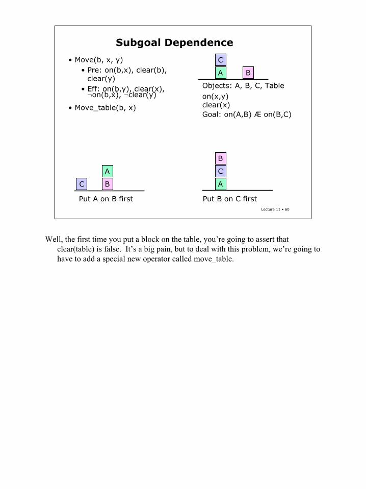
Well, the first time you put a block on the table, you’re going to assert that clear(table) is false. It’s a big pain, but to deal with this problem, we’re going to have to add a special new operator called move_table.
61
Lecture 11 • 61
Subgoal Dependence
• Move(b, x, y)• Pre: on(b,x), clear(b),
clear(y), block(y)• Eff: on(b,y), clear(x), ¬on(b,x), ¬clear(y)
• Move_table(b, x)
C
A B
Objects: A, B, C, Tableon(x,y)clear(x)Goal: on(A,B) Æ on(B,C)
C
A
B
C
A
B
Put A on B first Put B on C first
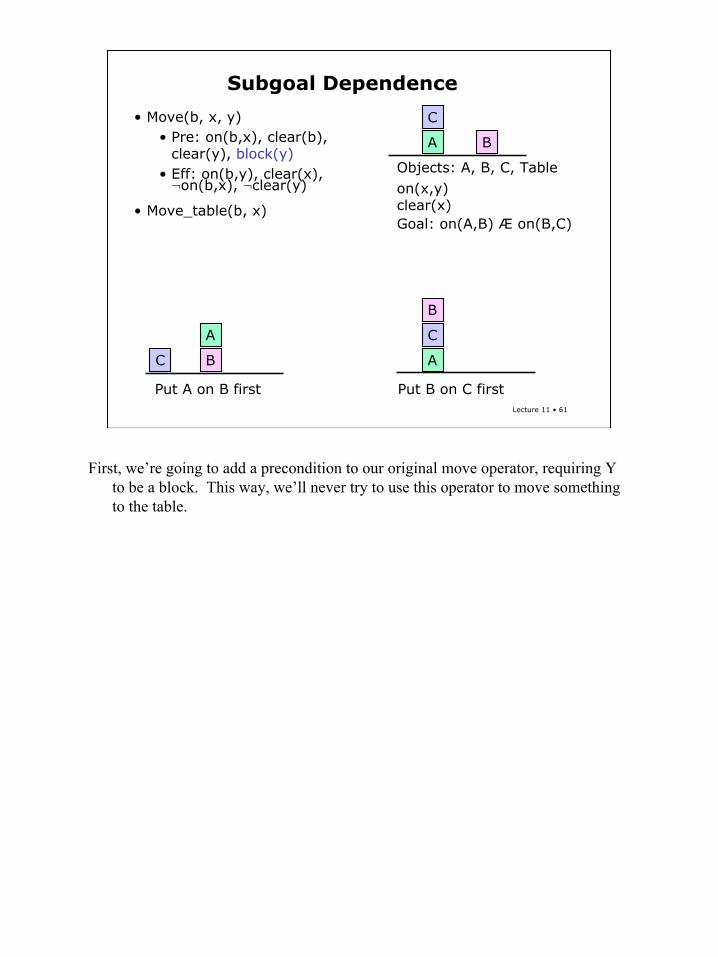
First, we’re going to add a precondition to our original move operator, requiring Y to be a block. This way, we’ll never try to use this operator to move something to the table.
62
Lecture 11 • 62
Subgoal Dependence
• Move(b, x, y)• Pre: on(b,x), clear(b),
clear(y), block(y)• Eff: on(b,y), clear(x), ¬on(b,x), ¬clear(y)
• Move_table(b, x)• Pre: on(b,x), clear(b)• Eff: on(b,table), clear(x), ¬on(b,x)
C
A B
Objects: A, B, C, Tableon(x,y)clear(x)Goal: on(A,B) Æ on(B,C)
C
A
B
C
A
B
Put A on B first Put B on C first
Then we’ll add the new operator just for moving a block B from X to the table. And the preconditions of that will be on (b,X), Clear(b) and that's all. And the effects will be on (b, table) and clear(X) and not on(B,X).
63
Lecture 11 • 63
Sussman Anomaly
start
clear(T) on(C,A) on(B,T) clear(C) clear(B)on(A,T)
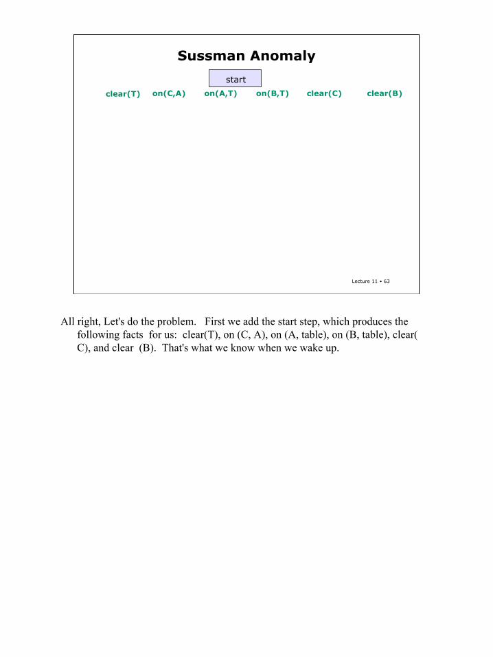
All right, Let's do the problem. First we add the start step, which produces the following facts for us: clear(T), on (C, A), on (A, table), on (B, table), clear( C), and clear (B). That's what we know when we wake up.
64
Lecture 11 • 64
Sussman Anomaly
start
clear(T) on(C,A) on(B,T) clear(C) clear(B)on(A,T)
finish
on(A,B) on(B,C)
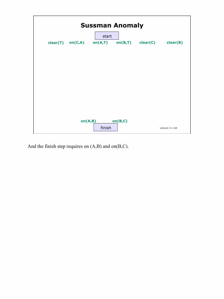
And the finish step requires on (A,B) and on(B,C).
65
Lecture 11 • 65
Sussman Anomaly
start
clear(T) on(C,A) on(B,T) clear(C) clear(B)on(A,T)
Move (A,x1,B)
finish
on(A,B) on(B,C)
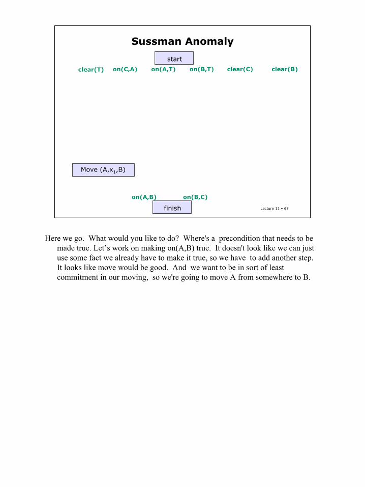
Here we go. What would you like to do? Where's a precondition that needs to be made true. Let’s work on making on(A,B) true. It doesn't look like we can just use some fact we already have to make it true, so we have to add another step. It looks like move would be good. And we want to be in sort of least commitment in our moving, so we're going to move A from somewhere to B.
66
Lecture 11 • 66
Sussman Anomaly
start
clear(T) on(C,A) on(B,T) clear(C) clear(B)on(A,T)
Move (A,x1,B)
on(A,B) ¬on(A,x1) clear (x1) ¬clear(B)
finish
on(A,B) on(B,C)
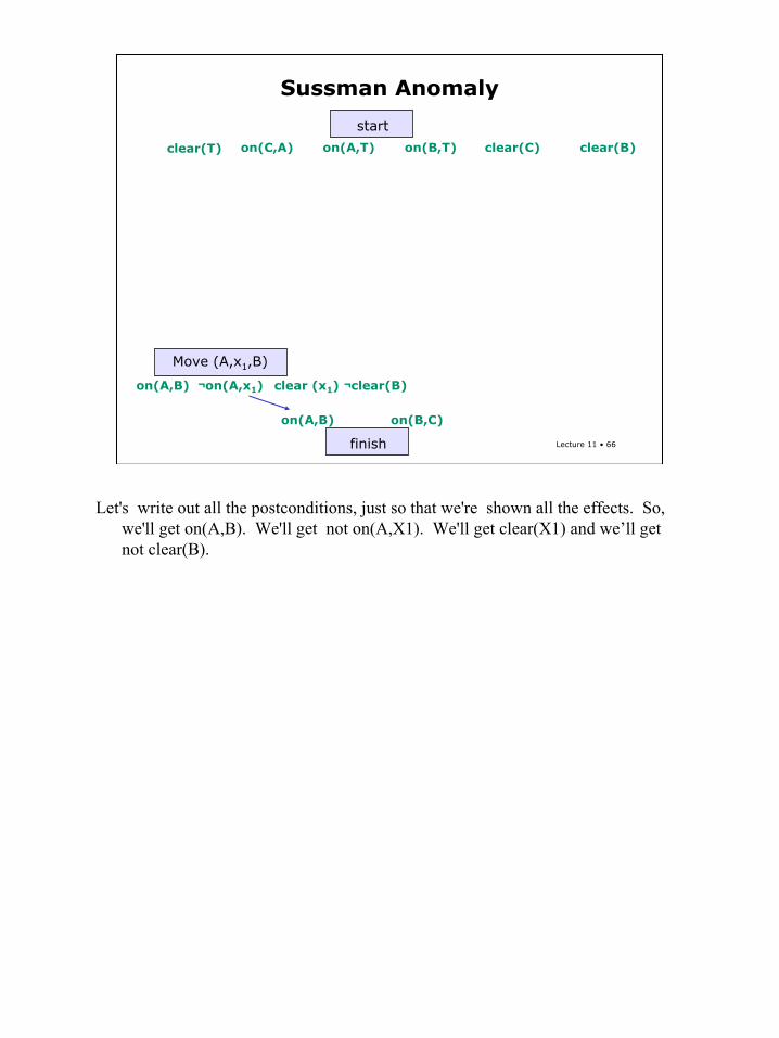
Let's write out all the postconditions, just so that we're shown all the effects. So, we'll get on(A,B). We'll get not on(A,X1). We'll get clear(X1) and we’ll get not clear(B).
67
Lecture 11 • 67
Sussman Anomaly
start
clear(T) on(C,A) on(B,T) clear(C) clear(B)on(A,T)
Move (A,x1,B)
on(A,x1) clear(A) clear(B)
on(A,B) ¬on(A,x1) clear (x1) ¬clear(B)
finish
on(A,B) on(B,C)
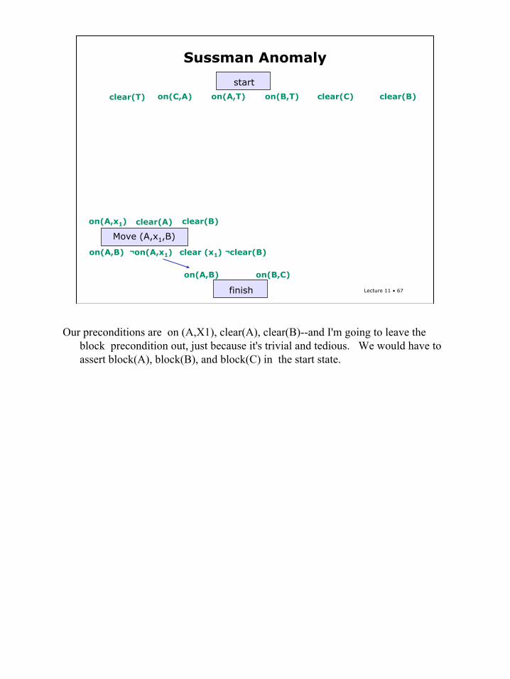
Our preconditions are on (A,X1), clear(A), clear(B)--and I'm going to leave the block precondition out, just because it's trivial and tedious. We would have to assert block(A), block(B), and block(C) in the start state.
68
Lecture 11 • 68
Sussman Anomaly
start
clear(T) on(C,A) on(B,T) clear(C) clear(B)on(A,T)
Move (A,x1,B)
on(A,x1) clear(A) clear(B)
on(A,B) ¬on(A,x1) clear (x1) ¬clear(B)
finish
on(A,B) on(B,C)
MoveT(y,A)
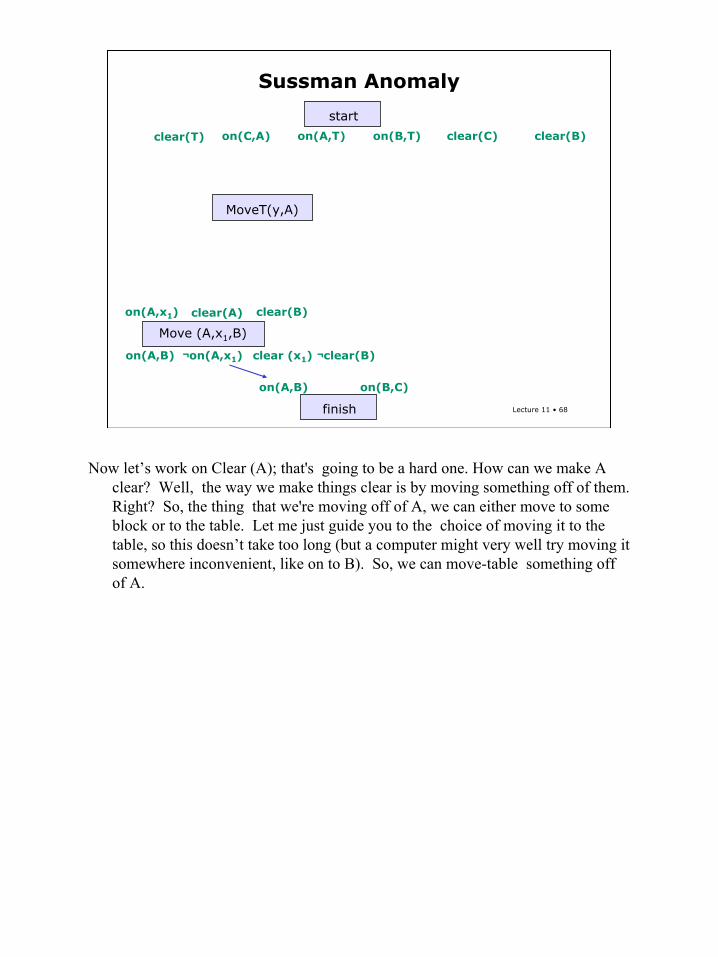
Now let’s work on Clear (A); that's going to be a hard one. How can we make A clear? Well, the way we make things clear is by moving something off of them. Right? So, the thing that we're moving off of A, we can either move to some block or to the table. Let me just guide you to the choice of moving it to the table, so this doesn’t take too long (but a computer might very well try moving it somewhere inconvenient, like on to B). So, we can move-table something off of A.
69
Lecture 11 • 69
Sussman Anomaly
start
clear(T) on(C,A) on(B,T) clear(C) clear(B)on(A,T)
Move (A,x1,B)
on(A,x1) clear(A) clear(B)
on(A,B) ¬on(A,x1) clear (x1) ¬clear(B)
finish
on(A,B) on(B,C)
MoveT(y,A)
on(y,T) clear(A) ¬on(y,A)
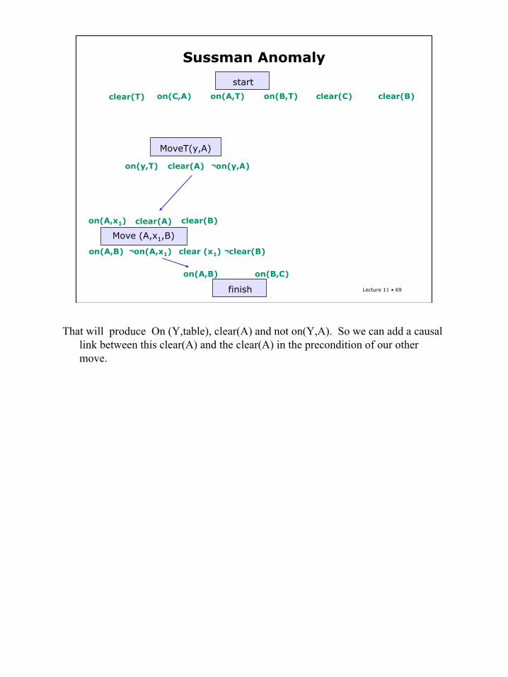
That will produce On (Y,table), clear(A) and not on(Y,A). So we can add a causal link between this clear(A) and the clear(A) in the precondition of our other move.
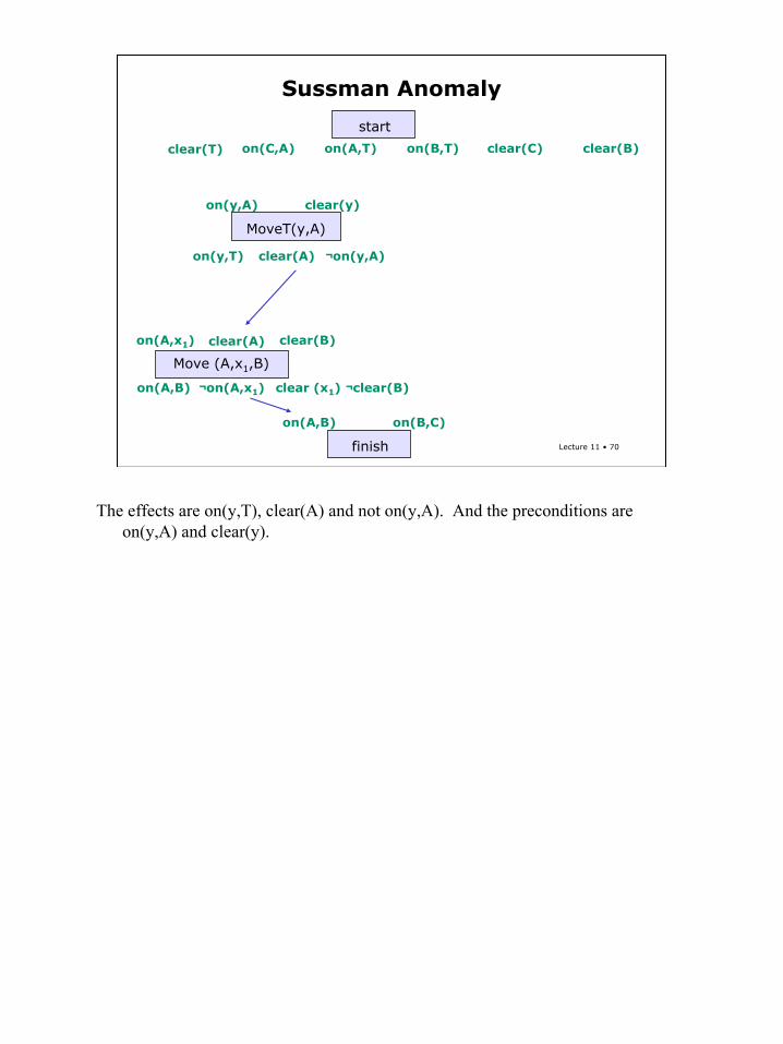
70
Lecture 11 • 70
Sussman Anomaly
start
clear(T) on(C,A) on(B,T) clear(C) clear(B)on(A,T)
Move (A,x1,B)
on(A,x1) clear(A) clear(B)
on(A,B) ¬on(A,x1) clear (x1) ¬clear(B)
finish
on(A,B) on(B,C)
MoveT(y,A)
on(y,A) clear(y)
on(y,T) clear(A) ¬on(y,A)
The effects are on(y,T), clear(A) and not on(y,A). And the preconditions are on(y,A) and clear(y).

71
Lecture 11 • 71
Sussman Anomaly
start
clear(T) on(C,A) on(B,T) clear(C) clear(B)on(A,T)
Move (A,x1,B)
on(A,x1) clear(A) clear(B)
on(A,B) ¬on(A,x1) clear (x1) ¬clear(B)
finish
on(A,B) on(B,C)
y=C
MoveT(y,A)
on(y,A) clear(y)
on(y,T) clear(A) ¬on(y,A)
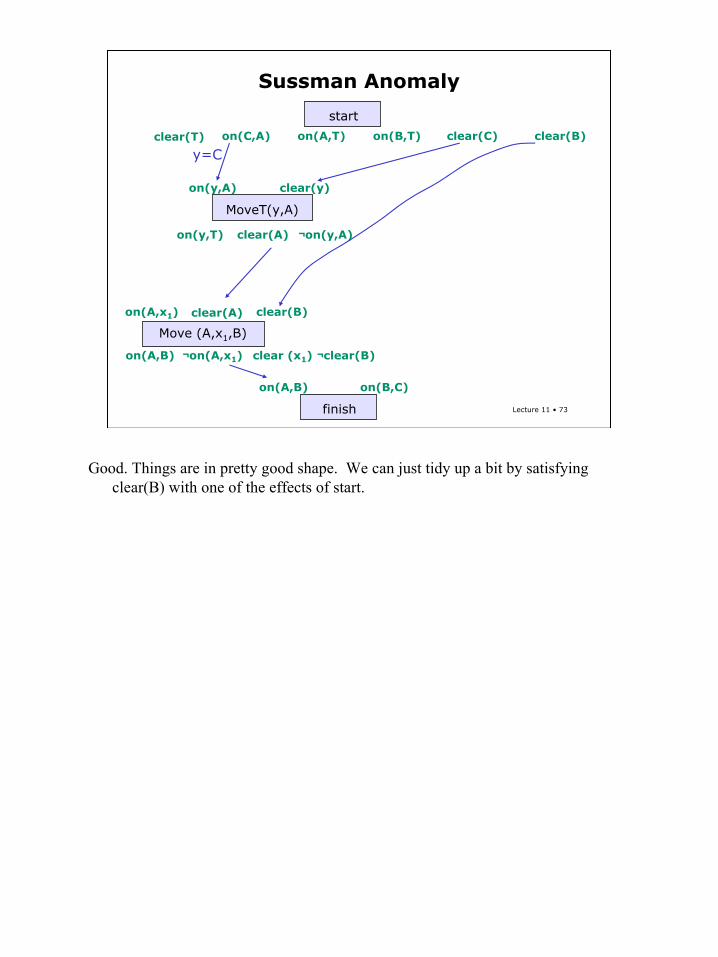
We can satisfy on(y,A) by letting y be C, and adding a causal connection from on(C,A) in the effects of start.

72
Lecture 11 • 72
Sussman Anomaly
start
clear(T) on(C,A) on(B,T) clear(C) clear(B)on(A,T)
Move (A,x1,B)
on(A,x1) clear(A) clear(B)
on(A,B) ¬on(A,x1) clear (x1) ¬clear(B)
finish
on(A,B) on(B,C)
y=C
MoveT(y,A)
on(y,A) clear(y)
on(y,T) clear(A) ¬on(y,A)
Since y is bound to C, we need clear C, which we can also find in the effects of start.
73
Lecture 11 • 73
Sussman Anomaly
start
clear(T) on(C,A) on(B,T) clear(C) clear(B)on(A,T)
Move (A,x1,B)
on(A,x1) clear(A) clear(B)
on(A,B) ¬on(A,x1) clear (x1) ¬clear(B)
finish
on(A,B) on(B,C)
y=C
MoveT(y,A)
on(y,A) clear(y)
on(y,T) clear(A) ¬on(y,A)
Good. Things are in pretty good shape. We can just tidy up a bit by satisfying clear(B) with one of the effects of start.
74
Lecture 11 • 74
Sussman Anomaly
start
clear(T) on(C,A) on(B,T) clear(C) clear(B)on(A,T)
Move (A,x1,B)
on(A,x1) clear(A) clear(B)
on(A,B) ¬on(A,x1) clear (x1) ¬clear(B)
finish
on(A,B) on(B,C)
y=C
x1=T
MoveT(y,A)
on(y,A) clear(y)
on(y,T) clear(A) ¬on(y,A)
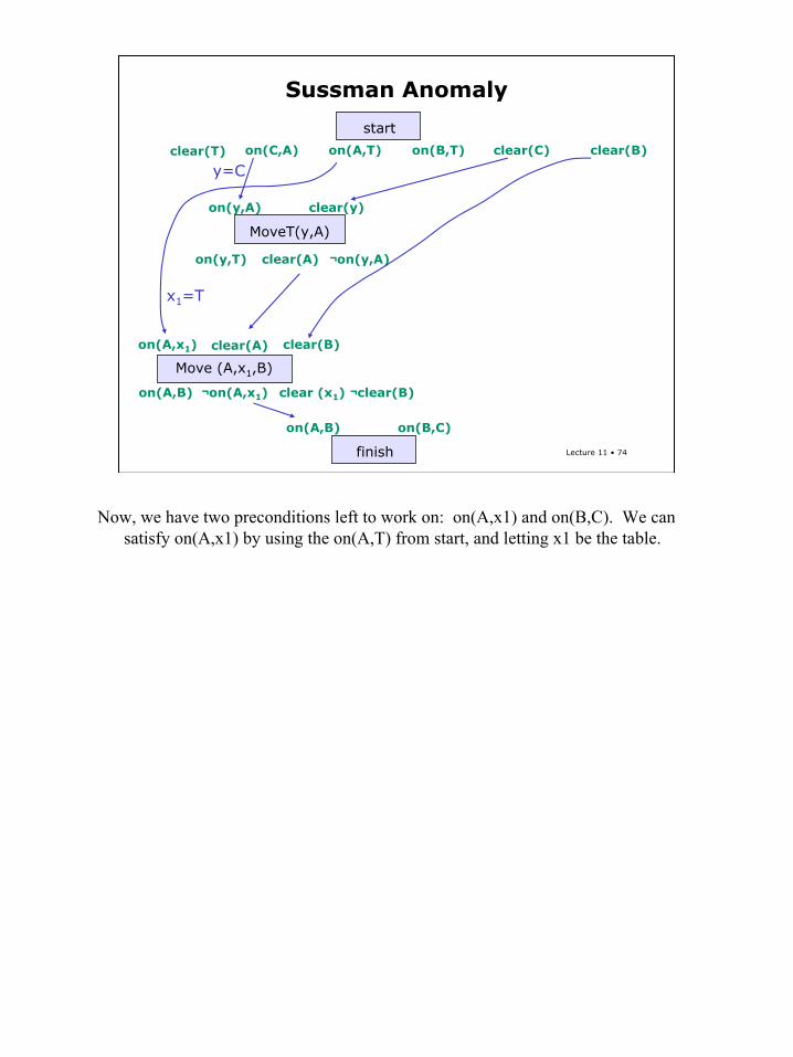
Now, we have two preconditions left to work on: on(A,x1) and on(B,C). We can satisfy on(A,x1) by using the on(A,T) from start, and letting x1 be the table.
75
Lecture 11 • 75
Sussman Anomaly
start
clear(T) on(C,A) on(B,T) clear(C) clear(B)on(A,T)
Move (A,x1,B)
on(A,x1) clear(A) clear(B)
on(A,B) ¬on(A,x1) clear (x1) ¬clear(B)
finish
on(A,B) on(B,C)
y=C
x1=T
MoveT(y,A)
on(y,A) clear(y)
on(y,T) clear(A) ¬on(y,A)
Move (B,x2,C)
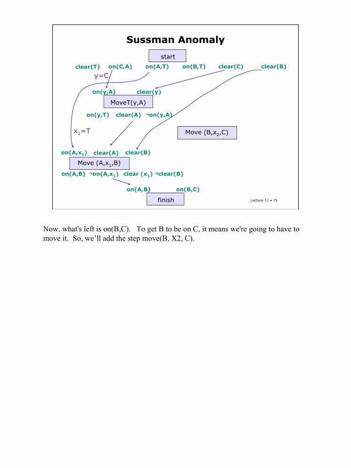
Now, what's left is on(B,C). To get B to be on C, it means we're going to have to move it. So, we’ll add the step move(B, X2, C).

76
Lecture 11 • 76
Sussman Anomaly
start
clear(T) on(C,A) on(B,T) clear(C) clear(B)on(A,T)
Move (A,x1,B)
on(A,x1) clear(A) clear(B)
on(A,B) ¬on(A,x1) clear (x1) ¬clear(B)
finish
on(A,B) on(B,C)
y=C
x1=T
MoveT(y,A)
on(y,A) clear(y)
on(y,T) clear(A) ¬on(y,A)
Move (B,x2,C)
on(B,x2) clear (B)
on(B,C) ¬on(B,x2) clear (x2) ¬clear(C)
clear (C)
That produces on(B,C), not on(B,x2), clear(x2) and not clear( C ). And it has as preconditions on(B,X2), clear(B), and clear(C).
77
Lecture 11 • 77
Sussman Anomaly
start
clear(T) on(C,A) on(B,T) clear(C) clear(B)on(A,T)
Move (A,x1,B)
on(A,x1) clear(A) clear(B)
on(A,B) ¬on(A,x1) clear (x1) ¬clear(B)
finish
on(A,B) on(B,C)
y=C
x1=T
x2=TMoveT(y,A)
on(y,A) clear(y)
on(y,T) clear(A) ¬on(y,A)
Move (B,x2,C)
on(B,x2) clear (B)
on(B,C) ¬on(B,x2) clear (x2) ¬clear(C)
clear (C)
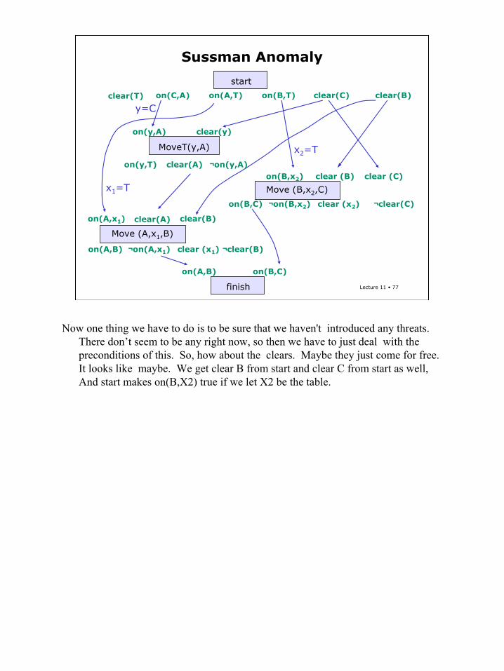
Now one thing we have to do is to be sure that we haven't introduced any threats. There don’t seem to be any right now, so then we have to just deal with the preconditions of this. So, how about the clears. Maybe they just come for free. It looks like maybe. We get clear B from start and clear C from start as well, And start makes on(B,X2) true if we let X2 be the table.
78
Lecture 11 • 78
Sussman Anomaly
start
clear(T) on(C,A) on(B,T) clear(C) clear(B)on(A,T)
Move (A,x1,B)
on(A,x1) clear(A) clear(B)
on(A,B) ¬on(A,x1) clear (x1) ¬clear(B)
finish
on(A,B) on(B,C)
y=C
x1=T
x2=TMoveT(y,A)
on(y,A) clear(y)
on(y,T) clear(A) ¬on(y,A)
Move (B,x2,C)
on(B,x2) clear (B)
on(B,C) ¬on(B,x2) clear (x2) ¬clear(C)
clear (C)
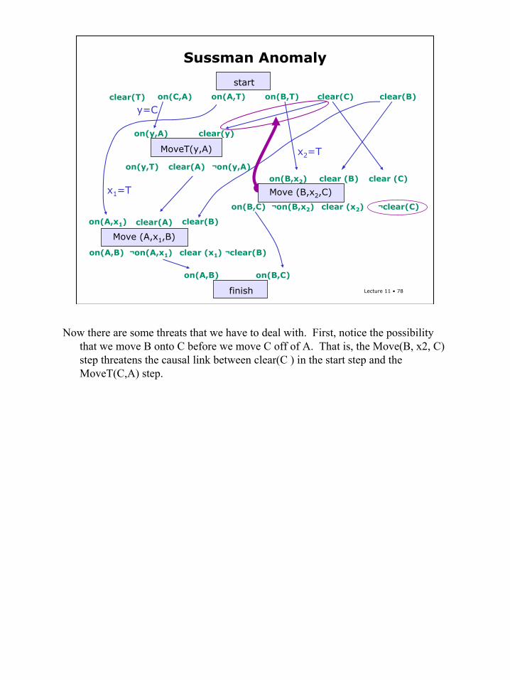
Now there are some threats that we have to deal with. First, notice the possibility that we move B onto C before we move C off of A. That is, the Move(B, x2, C) step threatens the causal link between clear(C ) in the start step and the MoveT(C,A) step.
79
Lecture 11 • 79
Sussman Anomaly
start
clear(T) on(C,A) on(B,T) clear(C) clear(B)on(A,T)
Move (A,x1,B)
on(A,x1) clear(A) clear(B)
on(A,B) ¬on(A,x1) clear (x1) ¬clear(B)
finish
on(A,B) on(B,C)
y=C
x1=T
x2=TMoveT(y,A)
on(y,A) clear(y)
on(y,T) clear(A) ¬on(y,A)
Move (B,x2,C)
on(B,x2) clear (B)
on(B,C) ¬on(B,x2) clear (x2) ¬clear(C)
clear (C)
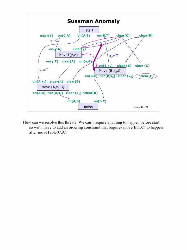
How can we resolve this threat? We can’t require anything to happen before start, so we’ll have to add an ordering constraint that requires move(B,T,C) to happen after moveTable(C,A).
80
Lecture 11 • 80
Sussman Anomaly
start
clear(T) on(C,A) on(B,T) clear(C) clear(B)on(A,T)
Move (A,x1,B)
on(A,x1) clear(A) clear(B)
on(A,B) ¬on(A,x1) clear (x1) ¬clear(B)
finish
on(A,B) on(B,C)
y=C
x1=T
x2=TMoveT(y,A)
on(y,A) clear(y)
on(y,T) clear(A) ¬on(y,A)
Move (B,x2,C)
on(B,x2) clear (B)
on(B,C) ¬on(B,x2) clear (x2) ¬clear(C)
clear (C)
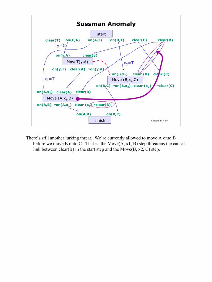
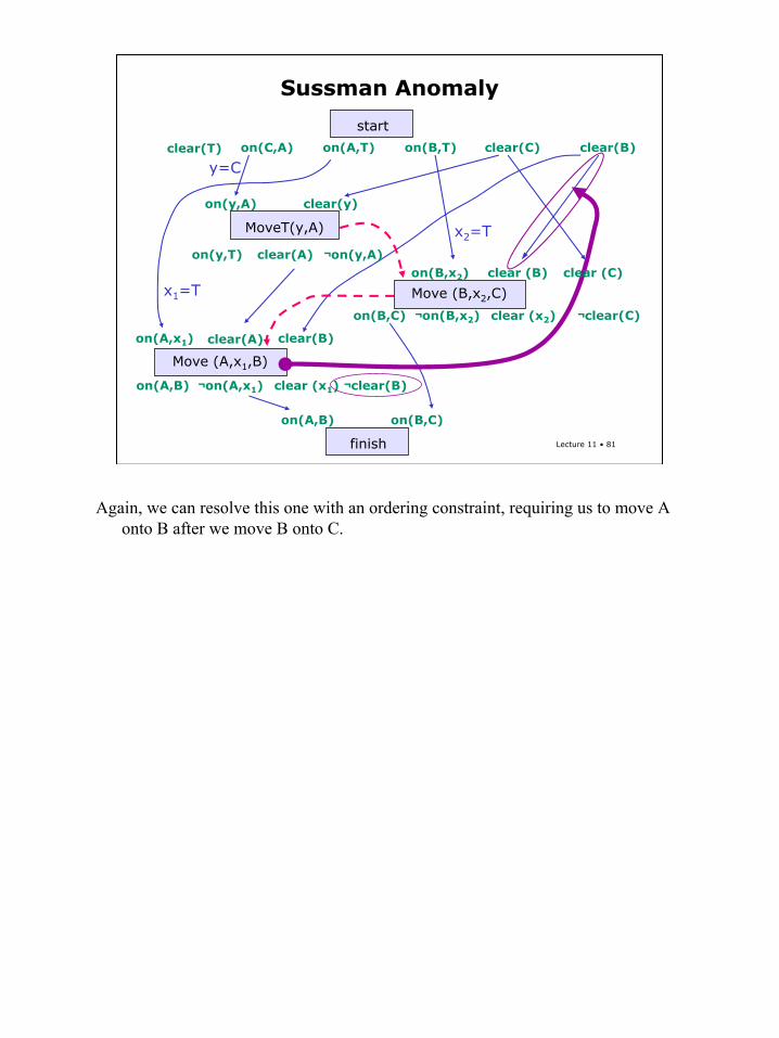
There’s still another lurking threat. We’re currently allowed to move A onto B before we move B onto C. That is, the Move(A, x1, B) step threatens the causal link between clear(B) in the start step and the Move(B, x2, C) step.
81
Lecture 11 • 81
Sussman Anomaly
start
clear(T) on(C,A) on(B,T) clear(C) clear(B)on(A,T)
Move (A,x1,B)
on(A,x1) clear(A) clear(B)
on(A,B) ¬on(A,x1) clear (x1) ¬clear(B)
finish
on(A,B) on(B,C)
y=C
x1=T
x2=TMoveT(y,A)
on(y,A) clear(y)
on(y,T) clear(A) ¬on(y,A)
Move (B,x2,C)
on(B,x2) clear (B)
on(B,C) ¬on(B,x2) clear (x2) ¬clear(C)
clear (C)
Again, we can resolve this one with an ordering constraint, requiring us to move A onto B after we move B onto C.
82
Lecture 11 • 82
Sussman Anomaly
start
clear(T) on(C,A) on(B,T) clear(C) clear(B)on(A,T)
Move (A,x1,B)
on(A,x1) clear(A) clear(B)
on(A,B) ¬on(A,x1) clear (x1) ¬clear(B)
finish
on(A,B) on(B,C)
y=C
x1=T
x2=TMoveT(y,A)
on(y,A) clear(y)
on(y,T) clear(A) ¬on(y,A)
Move (B,x2,C)
on(B,x2) clear (B)
on(B,C) ¬on(B,x2) clear (x2) ¬clear(C)
clear (C)
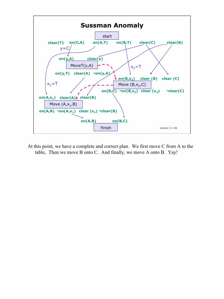
At this point, we have a complete and correct plan. We first move C from A to the table, Then we move B onto C. And finally, we move A onto B. Yay!

83
Lecture 11 • 83
Recitation Problems
• Russell & Norvig• 11.2• 11.7 a,b,c• 11.9
We can see the dependence of the subgoals quite clearly. We had to end up interleaving the steps required for each of the subgoals, in order to get a completely correct plan.