Embed Size (px)
Citation preview
A Partitioning-Centric Approach for the
Modeling and the Methodical Design of
Automotive Embedded Systems Architectures
Dissertation
A thesis submitted to the
Faculty of Electrical Engineering and Computer Sciencesof the
Technical University of Berlinin partial fulfillment of the requirements for the academical degree of
Dr.-Ing.
by
Augustin Kebemou
Berlin 2008D 83

ii

A Partitioning-Centric Approach for the
Modeling and the Methodical Design of
Automotive Embedded Systems Architectures
vorgelegt vonDipl.-Ing. Augustin Kebemou
Berlin
Von der Fakultat IV - Elektrotechnik und Informatik -der Technischen Universitat Berlin
zur Erlangung des akademischen Grades
Doktor der Ingenieurwissenschaften- Dr.-Ing. -
genehmigte Dissertation
Promotionsausschuss:
- Prof. Dr.Sabine Glesner (Vorsitzender)- Prof. Dr.-Ing. Ina Schieferdecker (Gutachter)- Prof. Dr. Jakob Rehof (Gutachter)
Tag der wissenschaftlichen Aussprache: 06.05.2008
Berlin 2008D 83

ii

Acknowledgments
”Acquiring knowledge is useless unless it makes us better servants of humanity”.The achievement of this thesis would not have been possible without the intervention and the
support of many people. I am very grateful to all those who supported me during the work thatled to this thesis.
In particular, I would like to thank the supervisor of this work, Prof. Dr.-Ing. Ina Schieferdecker(holder of the chair for Design and Testing of Telecommunication Systems at the TU Berlin andconcurrently leader of the research group MOTION at the Fraunhofer Institute FOKUS) for heradvices, for her reviews and her suggestions that improved both the technical and the scientificquality of this thesis. I also thank Ina for the friendly working atmosphere that gave me additionalself-confidence to go ahead.
I am also deeply grateful to Prof. Dr. Jakob Rehof, the director of the Fraunhofer Institutefor Software and Systems Engineering (ISST) and concurrently holder of the chair for SoftwareEngineering at the university of Dortmund, who accepted spontaneously to support me, invested histime to examine my work and undertook the co-supervision activities that considerably contributedto the achievement of this thesis.
Taking this opportunity, I would further like to thank Rainer Mackenthun, the head of theDepartment of Dependable Technical Systems at the Fraunhofer Institute for Software and SystemsEngineering (ISST) in Berlin, Prof. Dr. Herbert Weber, Dr. Alexander Borusan and Dr. VolkerZurwehn, also from the ISST institute in Berlin, for their psychological support. I did appreciateyour fairness and the way you judged my work during my hard days.
I would also like to address my special thanks to Angelika Becker, who played a central role inthe accomplishment of this thesis. Thank you very much, Geli, for the nights and the weekendsyou spent to review this thesis and to correct my textual formulations. Thank you for your advices.Thank you for the time you invested in intensive discussions with me. Thank you once more foryour emotional support.
I finally wish to express my gratefulness to my family and all of my friends for their patienceduring the years of this thesis as well as to my colleagues at the Fraunhofer Institute for Softwareand Systems Engineering (ISST) who participated in the fruitful discussions that made this thesispossible.
Thank u all.
Once more, remember: ”Acquiring knowledge is useless unless it makes you a better servantof humanity”.
A. Kebemou
i

ii

Abstract
Because of the increasing demand for more comfort, security and environmental compatibility,the development of E/E-systems (Electric/Electronic) has become a central task for automobilemanufacturers. In the actual context that is characterized by the rapid increase of software- andelectronic-based components in modern vehicles and the related hard competition in the automobilemarket, it is necessary to design optimal architectures for automobiles’ E/E-systems in a relativelyshort time. An optimal architecture of an E/E-system must minimize the usage of the hardware(i.e. processing units, memory elements, communication cables, etc.) as well as the operatingcosts (energy and fuel consumption, maintenance, waste disposal, etc.) and concurrently optimizethe functioning and the quality (i.e. performance, reliability, safety, security, etc.) of the system.In this thesis we suggest to solve this problem by means of CAD-supported tools. This requiresdrastic changes within both the established development methods and the design processes. Wepropose a system-oriented design process and an automatic partitioning method with appropriatemodeling techniques to support the model-based definition of the architectures of automobiles’E/E-systems.
Abstrakt (Deutsch)
Vor dem Hintergrund der steigenden Nachfrage nach mehr Komfort, Sicherheit und Umweltfre-undlichkeit ist die Entwicklung von E/E-Systemen (elektrik/elektronik) zu einer zentralen Auf-gabe fur die Automobilhersteller geworden. In der gegenwartigen Situation, die durch die rapideZunahme von software- und elektronikbasierten Bestandteilen in modernen Fahrzeugen und dendamit verbundenen harten Konkurrenzkampf auf dem Automobilmarkt gekennzeichnet ist, ist esnotwendig, optimale Architekturen fur automobile E/E-Systeme in relativ kurzer Zeit zu entwickeln.Die optimale Architektur eines E/E-Systems muss die Hardwarenutzung (d. h. Prozessoren, Daten-speicher, Kommunikationskabel, I/O Module, etc.) und die Betriebskosten (Energie- und Treibstof-fverbrauch, Wartung, Verschrottung, etc.) verringern und gleichzeitig die Funktionstuchtigkeit unddie Qualitat (Leistung, Zuverlassigkeit, Sicherheit, etc.) des Systems verbessern. In dieser Arbeitschlagen wir vor, dieses Problem durch computergestutzte Werkzeuge zu losen. Dies macht ein-schneidende Veranderungen sowohl in den Entwicklungsmethoden als auch in den Designprozessenerforderlich. Wir schlagen einen systemorientierten Entwicklungsprozess vor, der die modellbasierteDefinition der Architekturen von automobilen E/E-Systemen unterstutzen kann. Diese Arbeitdefiniert die passenden Modellierungstechniken und die Algorithmen, die eine automatische Parti-tionierung von System-level-E/E-Modellen ermoglichen.
iii

iv
Contents
1 General introduction 1
1.1 Motivation . . . . . . . . . . . . . . . . . . . . . . . . . . . . . . . . . . . . . . . 11.2 Problem definition . . . . . . . . . . . . . . . . . . . . . . . . . . . . . . . . . . . 31.3 Procedural method to solve the problem . . . . . . . . . . . . . . . . . . . . . . . 91.4 Contributions . . . . . . . . . . . . . . . . . . . . . . . . . . . . . . . . . . . . . 121.5 Publications . . . . . . . . . . . . . . . . . . . . . . . . . . . . . . . . . . . . . . 131.6 Scheduling of the thesis . . . . . . . . . . . . . . . . . . . . . . . . . . . . . . . . 13
2 Automotive Embedded Systems 15
2.1 Automotive electronics . . . . . . . . . . . . . . . . . . . . . . . . . . . . . . . . 152.1.1 Embedded systems . . . . . . . . . . . . . . . . . . . . . . . . . . . . . . 152.1.2 Automotive and embedded systems . . . . . . . . . . . . . . . . . . . . . 162.1.3 Example: The Active Cruise Control . . . . . . . . . . . . . . . . . . . . . 172.1.4 The ACC functional connectivity . . . . . . . . . . . . . . . . . . . . . . . 19
2.2 Automotive connectivity . . . . . . . . . . . . . . . . . . . . . . . . . . . . . . . . 192.2.1 Automotive communication protocols . . . . . . . . . . . . . . . . . . . . 192.2.2 All-rounder automotive communication protocols . . . . . . . . . . . . . . 202.2.3 High-speed and real-time protocols . . . . . . . . . . . . . . . . . . . . . . 212.2.4 General-purpose protocols . . . . . . . . . . . . . . . . . . . . . . . . . . . 232.2.5 Other in-vehicle and smart network protocols . . . . . . . . . . . . . . . . 24
2.3 Conclusion . . . . . . . . . . . . . . . . . . . . . . . . . . . . . . . . . . . . . . . 25
3 Embedded systems design 27
3.1 Embedded systems design methods . . . . . . . . . . . . . . . . . . . . . . . . . . 273.1.1 The sequential design process . . . . . . . . . . . . . . . . . . . . . . . . . 273.1.2 The concurrent design method . . . . . . . . . . . . . . . . . . . . . . . . 28
3.2 Design activities . . . . . . . . . . . . . . . . . . . . . . . . . . . . . . . . . . . . 293.2.1 The specification . . . . . . . . . . . . . . . . . . . . . . . . . . . . . . . 293.2.2 The partitioning . . . . . . . . . . . . . . . . . . . . . . . . . . . . . . . . 29
3.3 The implementation . . . . . . . . . . . . . . . . . . . . . . . . . . . . . . . . . . 303.3.1 The software synthesis . . . . . . . . . . . . . . . . . . . . . . . . . . . . 303.3.2 The hardware synthesis . . . . . . . . . . . . . . . . . . . . . . . . . . . . 313.3.3 The synthesis of the interfaces . . . . . . . . . . . . . . . . . . . . . . . . 32
3.4 Conclusion . . . . . . . . . . . . . . . . . . . . . . . . . . . . . . . . . . . . . . . 32
4 Automotive systems design 35
4.1 Design of AES . . . . . . . . . . . . . . . . . . . . . . . . . . . . . . . . . . . . . 354.1.1 Top-down and bottom-up . . . . . . . . . . . . . . . . . . . . . . . . . . . 354.1.2 Current OEM design practice . . . . . . . . . . . . . . . . . . . . . . . . . 354.1.3 Limitations of the current OEM design practice . . . . . . . . . . . . . . . 36
4.2 Proposed design approach . . . . . . . . . . . . . . . . . . . . . . . . . . . . . . . 374.2.1 Factors of the problem resolution . . . . . . . . . . . . . . . . . . . . . . . 37
v
vi CONTENTS
4.2.2 The system-oriented design approach . . . . . . . . . . . . . . . . . . . . . 384.2.3 Analysis . . . . . . . . . . . . . . . . . . . . . . . . . . . . . . . . . . . . 39
4.3 Conclusion . . . . . . . . . . . . . . . . . . . . . . . . . . . . . . . . . . . . . . . 40
5 Modeling AES: State-of-the-art 415.1 Modeling AES . . . . . . . . . . . . . . . . . . . . . . . . . . . . . . . . . . . . . 41
5.1.1 Model-driven system development in the automotive engineering . . . . . . 415.1.2 AES are heterogeneous and complex systems . . . . . . . . . . . . . . . . 42
5.2 AES modeling needs . . . . . . . . . . . . . . . . . . . . . . . . . . . . . . . . . . 425.2.1 AES modeling prerequisites . . . . . . . . . . . . . . . . . . . . . . . . . . 425.2.2 Features expected from an AES model-based design solution . . . . . . . . 43
5.3 AES basic modeling concepts . . . . . . . . . . . . . . . . . . . . . . . . . . . . . 445.3.1 Abstraction levels in the AES design . . . . . . . . . . . . . . . . . . . . . 445.3.2 AES architectural modeling concepts . . . . . . . . . . . . . . . . . . . . . 455.3.3 AES behavioral modeling concepts . . . . . . . . . . . . . . . . . . . . . . 47
5.4 Conclusion . . . . . . . . . . . . . . . . . . . . . . . . . . . . . . . . . . . . . . . 48
6 The value of AES modeling languages 496.1 The evaluation framework . . . . . . . . . . . . . . . . . . . . . . . . . . . . . . . 49
6.1.1 AES modeling requirements for the partitioning . . . . . . . . . . . . . . . 496.1.2 Related work . . . . . . . . . . . . . . . . . . . . . . . . . . . . . . . . . . 506.1.3 Classification criteria . . . . . . . . . . . . . . . . . . . . . . . . . . . . . 516.1.4 Criteria for evaluating the level of support . . . . . . . . . . . . . . . . . . 53
6.2 AES modeling languages . . . . . . . . . . . . . . . . . . . . . . . . . . . . . . . 556.2.1 General-purpose languages . . . . . . . . . . . . . . . . . . . . . . . . . . 556.2.2 Automotive domain-specific modeling languages . . . . . . . . . . . . . . . 58
6.3 Evaluation and classification of AES modeling languages . . . . . . . . . . . . . . 616.4 Conclusion . . . . . . . . . . . . . . . . . . . . . . . . . . . . . . . . . . . . . . . 62
7 Inputs for the partitioning 677.1 Required inputs for the partitioning . . . . . . . . . . . . . . . . . . . . . . . . . . 677.2 Specifying the system’s functionalities . . . . . . . . . . . . . . . . . . . . . . . . 68
7.2.1 Relevant modeling concepts . . . . . . . . . . . . . . . . . . . . . . . . . . 687.2.2 The FN: The modeling solution for the functional specification . . . . . . 69
7.3 Specifying the hardware platform . . . . . . . . . . . . . . . . . . . . . . . . . . . 727.3.1 Relevant modeling concepts . . . . . . . . . . . . . . . . . . . . . . . . . . 727.3.2 The HN: The hardware platform . . . . . . . . . . . . . . . . . . . . . . . 75
7.4 The partitioning . . . . . . . . . . . . . . . . . . . . . . . . . . . . . . . . . . . . 757.4.1 Formal definition of the partitioning problem . . . . . . . . . . . . . . . . . 757.4.2 Relevant attributes for the elements of the input models . . . . . . . . . . 77
7.5 Conclusion . . . . . . . . . . . . . . . . . . . . . . . . . . . . . . . . . . . . . . . 79
8 The synthesis Model 818.1 Definition of the synthesis model . . . . . . . . . . . . . . . . . . . . . . . . . . . 81
8.1.1 Requirements for the synthesis model . . . . . . . . . . . . . . . . . . . . 818.1.2 The synthesis model . . . . . . . . . . . . . . . . . . . . . . . . . . . . . . 82
8.2 Annotations for the synthesis model . . . . . . . . . . . . . . . . . . . . . . . . . 858.2.1 Concurrency, sequencing . . . . . . . . . . . . . . . . . . . . . . . . . . . 858.2.2 Annotations for the nodes . . . . . . . . . . . . . . . . . . . . . . . . . . . 858.2.3 Annotations for the edges . . . . . . . . . . . . . . . . . . . . . . . . . . . 868.2.4 Annotations for the tokens . . . . . . . . . . . . . . . . . . . . . . . . . . 868.2.5 Formal definition of the synthesis model . . . . . . . . . . . . . . . . . . . 87
8.3 Applications . . . . . . . . . . . . . . . . . . . . . . . . . . . . . . . . . . . . . . 88

CONTENTS vii
8.3.1 The weight of an edge in a CDFM model . . . . . . . . . . . . . . . . . . 888.3.2 Model transformation . . . . . . . . . . . . . . . . . . . . . . . . . . . . . 89
8.4 Conclusion . . . . . . . . . . . . . . . . . . . . . . . . . . . . . . . . . . . . . . . 89
9 The partitioning: State-of-the-art 91
9.1 The partitioning problem . . . . . . . . . . . . . . . . . . . . . . . . . . . . . . . 919.1.1 Frames of the problem . . . . . . . . . . . . . . . . . . . . . . . . . . . . 919.1.2 Requirements for the partitioning algorithm . . . . . . . . . . . . . . . . . 92
9.2 Partitioning methods . . . . . . . . . . . . . . . . . . . . . . . . . . . . . . . . . 939.2.1 Exact and heuristic methods . . . . . . . . . . . . . . . . . . . . . . . . . 939.2.2 Constructive partitioning techniques . . . . . . . . . . . . . . . . . . . . . 959.2.3 Iterative improvement techniques . . . . . . . . . . . . . . . . . . . . . . . 97
9.3 Conclusion . . . . . . . . . . . . . . . . . . . . . . . . . . . . . . . . . . . . . . . 101
10 The partitioning algorithms 103
10.1 The partitioning strategy . . . . . . . . . . . . . . . . . . . . . . . . . . . . . . . 10310.1.1 A three-step process . . . . . . . . . . . . . . . . . . . . . . . . . . . . . . 10310.1.2 Definitions of terms . . . . . . . . . . . . . . . . . . . . . . . . . . . . . . 10410.1.3 The main procedure . . . . . . . . . . . . . . . . . . . . . . . . . . . . . . 105
10.2 The pre-clustering . . . . . . . . . . . . . . . . . . . . . . . . . . . . . . . . . . . 10510.2.1 Definition . . . . . . . . . . . . . . . . . . . . . . . . . . . . . . . . . . . 10510.2.2 The pre-clustering algorithm . . . . . . . . . . . . . . . . . . . . . . . . . 106
10.3 The clustering . . . . . . . . . . . . . . . . . . . . . . . . . . . . . . . . . . . . . 10710.3.1 Closeness metrics . . . . . . . . . . . . . . . . . . . . . . . . . . . . . . . 10710.3.2 The closeness function . . . . . . . . . . . . . . . . . . . . . . . . . . . . 11010.3.3 The QT clustering algorithm . . . . . . . . . . . . . . . . . . . . . . . . . 11110.3.4 Conclusion . . . . . . . . . . . . . . . . . . . . . . . . . . . . . . . . . . . 113
11 Evaluating and improving a partition 115
11.1 The CAN: A frame-oriented communication protocol . . . . . . . . . . . . . . . . 11511.1.1 Organization of a CAN network . . . . . . . . . . . . . . . . . . . . . . . 11511.1.2 CAN frames . . . . . . . . . . . . . . . . . . . . . . . . . . . . . . . . . . 11611.1.3 Format of a standard CAN data frame . . . . . . . . . . . . . . . . . . . . 11611.1.4 Frames multiplexing . . . . . . . . . . . . . . . . . . . . . . . . . . . . . . 11711.1.5 Relations with the partitioning . . . . . . . . . . . . . . . . . . . . . . . . 11911.1.6 Practical considerations for the frames multiplexing . . . . . . . . . . . . . 119
11.2 The value of a partition . . . . . . . . . . . . . . . . . . . . . . . . . . . . . . . . 12111.2.1 The cost function . . . . . . . . . . . . . . . . . . . . . . . . . . . . . . . 12111.2.2 The cost as a bin packing problem . . . . . . . . . . . . . . . . . . . . . . 122
11.3 Bin packing techniques . . . . . . . . . . . . . . . . . . . . . . . . . . . . . . . . 12311.3.1 The Next Fit, the First Fit and the Best Fit strategies . . . . . . . . . . . 12311.3.2 Off-line packing strategies . . . . . . . . . . . . . . . . . . . . . . . . . . . 124
11.4 Investigating the cost of a partition . . . . . . . . . . . . . . . . . . . . . . . . . . 12511.4.1 The FFD strategy for the cost estimation . . . . . . . . . . . . . . . . . . 12511.4.2 The frames packing algorithm for the cost investigation . . . . . . . . . . . 126
11.5 Improving the partition . . . . . . . . . . . . . . . . . . . . . . . . . . . . . . . . 12711.5.1 The Kernighan & Lin strategy . . . . . . . . . . . . . . . . . . . . . . . . 12711.5.2 The improvement technique . . . . . . . . . . . . . . . . . . . . . . . . . 12811.5.3 The improvement procedure . . . . . . . . . . . . . . . . . . . . . . . . . 130
11.6 Conclusion . . . . . . . . . . . . . . . . . . . . . . . . . . . . . . . . . . . . . . . 132

viii CONTENTS
12 Applications 13312.1 The application case . . . . . . . . . . . . . . . . . . . . . . . . . . . . . . . . . . 133
12.1.1 Presentation of the application case . . . . . . . . . . . . . . . . . . . . . 13312.1.2 Objectives and scenario . . . . . . . . . . . . . . . . . . . . . . . . . . . . 134
12.2 The investigation . . . . . . . . . . . . . . . . . . . . . . . . . . . . . . . . . . . 13512.2.1 The models . . . . . . . . . . . . . . . . . . . . . . . . . . . . . . . . . . 13512.2.2 The attributes of the tokens . . . . . . . . . . . . . . . . . . . . . . . . . 13712.2.3 The partitioning . . . . . . . . . . . . . . . . . . . . . . . . . . . . . . . . 139
12.3 Results . . . . . . . . . . . . . . . . . . . . . . . . . . . . . . . . . . . . . . . . . 13912.4 Conclusion . . . . . . . . . . . . . . . . . . . . . . . . . . . . . . . . . . . . . . . 140
13 General conclusion 14113.1 Summary . . . . . . . . . . . . . . . . . . . . . . . . . . . . . . . . . . . . . . . . 14113.2 Outlook . . . . . . . . . . . . . . . . . . . . . . . . . . . . . . . . . . . . . . . . 145
A Zusammenfassung der Dissertation 1A.1 Motivation . . . . . . . . . . . . . . . . . . . . . . . . . . . . . . . . . . . . . . . 1A.2 Problemlosung . . . . . . . . . . . . . . . . . . . . . . . . . . . . . . . . . . . . . 3A.3 Wissenschaftliche Beitrage der Dissertation . . . . . . . . . . . . . . . . . . . . . 5
Glossary of Terms and Abbreviations i
List of Figures v
List of Algorithms vii
List of Tables ix
Bibliography xi

Chapter 1
General introduction
In this chapter we give a general presentation of this thesis. Beginning with the genesis of the problemthat is to be solved, we define the concerns of our work and we provide an overview of our solutionschemata. The problem of finding a CAD-supported partitioning method that is applicable to system-level specifications of automotive embedded systems (AES) is elucidated and its necessity for today’sdesign process of AES is justified. The following problem definition clarifies the purpose and the goalof our investigations. It also describes the scope of this thesis. We then provide our solution schemataand an outlook on the possible expansions and the usability of the solutions.
1.1 Motivation
Today’s vehicle manufacturers must produce pretty, reliable, safe-functioning vehicles with powerfulengines, robust mechanics and high comfort, all that in mass-production, where stringent qualityrequirements go together with the demand for low costs and low maintenance needs, but highsafety and security levels, high dependability, absolute reliability and short time-to-market. Thereto,vehicles underlie severe legal constraints such as the required environmental compatibility prescribedfor example in [3–5]. Sophisticated embedded electronic controllers are used to cope with theseconstraints and to satisfy the steadily increasing expectations of the consumers. In this context, thequantity of automotive electronic- and software-based functionalities is likely to grow continuously,requiring efficient development and production methodologies to continue to build high-quality andcost sensitive vehicles. The required methodologies must not only assure the best product quality,but they must also facilitate the maintenance and finally the disposal of the resulting vehicles andincrease the productivity of the vehicle manufacturers.
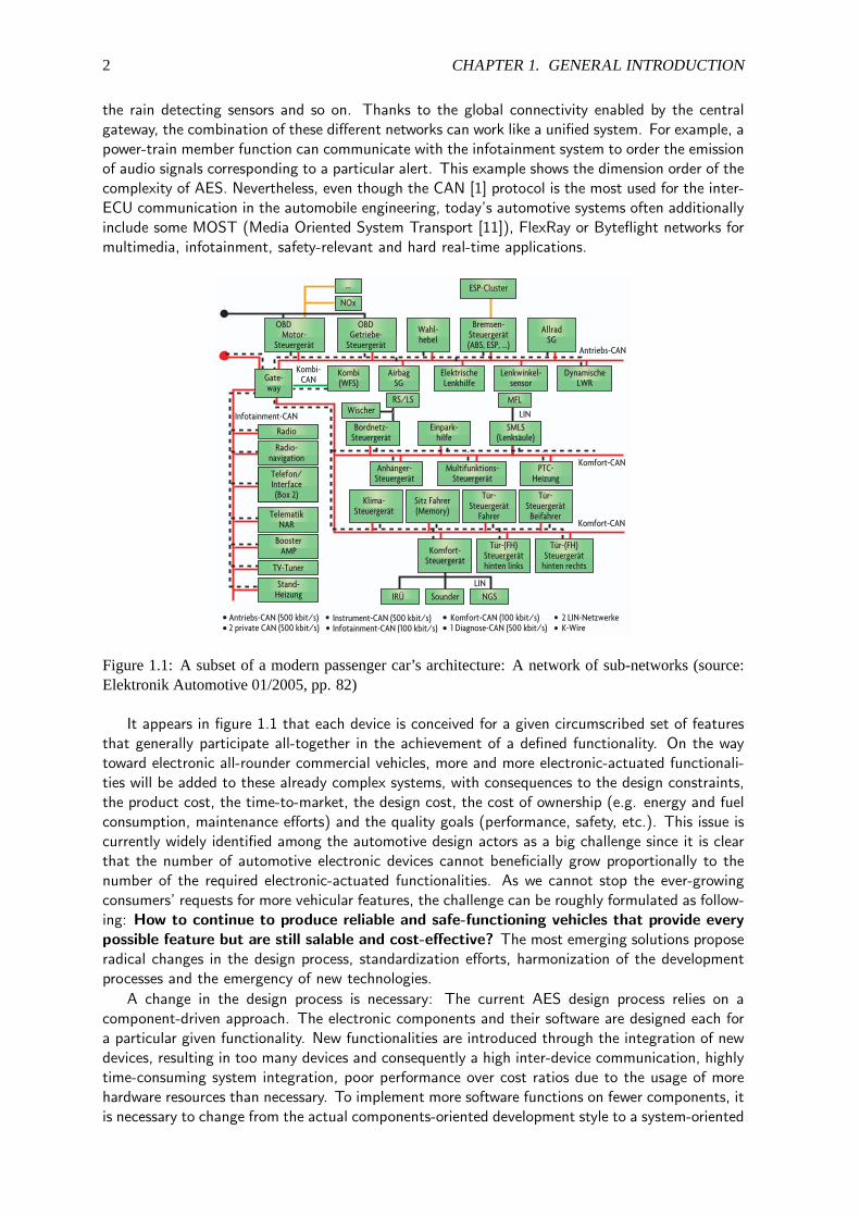
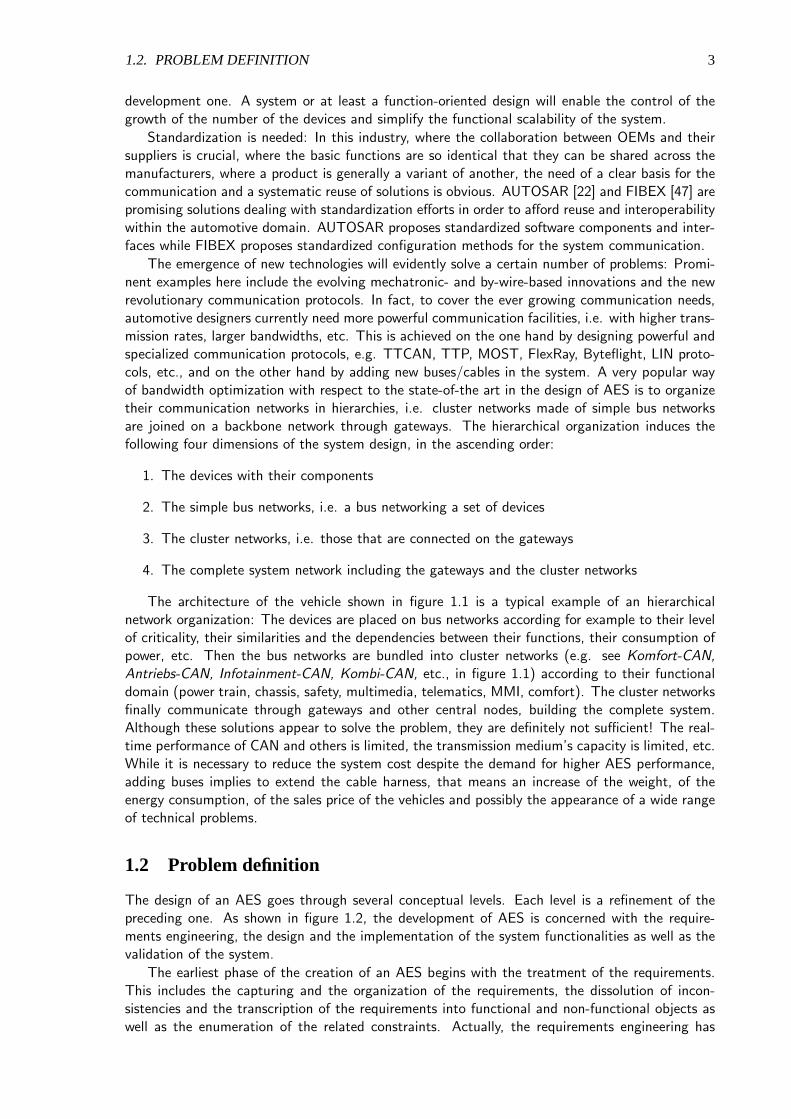
Automotive systems are actually very complex systems the software-based functionalities ofwhich are distributed on several embedded components including electronic control units (ECU),sensors and actuators which do not only cooperate with each other, but also depend on each other.Figure 1.1 shows the typical architecture of the platform of a modern personal vehicle. In thiscar, there are five high-speed CAN (Controller Area Network) networks operating at 500 kbit/s:The power-train bus, called ”Antrieb-CAN” in the figure, networks the engine, the gearbox, thetransmission, the airbags, the all-wheel controller units and several braking, stability and steeringassistance controllers. Another high-speed CAN bus connects the instrumentations controller(”Kombi” in the figure) with the rest of the system through the central gateway while the carexhaust management system (”NOx,...”) uses the engine controller as gateway to the other partsof the system. This complex system around the high-speed CAN also includes the ESP-Cluster andthe diagnosis bus (i.e. the one enclosed by dotted lines) that feeds the entire system. Concurrently,a low-speed CAN protocol running at 100 kbit/s is implemented for the infotainment and othercomfort functions (here ”Komfort-CAN”). In addition, the system runs two LIN networks. LINstands for Local Interconnect Network [10]. The first LIN network clusters the multi-functionalsteering wheel sensing system (“MFL”) and the second one interconnects the wipers, the mirrors,
1
2 CHAPTER 1. GENERAL INTRODUCTION
the rain detecting sensors and so on. Thanks to the global connectivity enabled by the centralgateway, the combination of these different networks can work like a unified system. For example, apower-train member function can communicate with the infotainment system to order the emissionof audio signals corresponding to a particular alert. This example shows the dimension order of thecomplexity of AES. Nevertheless, even though the CAN [1] protocol is the most used for the inter-ECU communication in the automobile engineering, today’s automotive systems often additionallyinclude some MOST (Media Oriented System Transport [11]), FlexRay or Byteflight networks formultimedia, infotainment, safety-relevant and hard real-time applications.
LIN
Kombi-CAN
Infotainment-CAN
LIN
Komfort-CAN
Komfort-CAN
Antriebs-CAN
Antriebs-CAN (500 kbit/s)2 private CAN (500 kbit/s)
Telefon/Interface(Box 2)
Radio-navigation
Bordnetz-Steuergerät
Einpark-hilfe
Multifunktions-Steuergerät
Anhänger-Steuergerät
PTC-Heizung
SMLS(Lenksäule)
Kombi(WFS)
AirbagSG
ElektrischeLenkhilfe
Lenkwinkel-sensor
DynamischeLWR
TelematikNAR
BoosterAMP
Stand-Heizung
Radio
NOx
...
Sounder NGSIRÜ
WischerRS/LS MFL
TV-Tuner
Bremsen-Steuergerät(ABS, ESP, ...)
ESP-Cluster
Tür-Steuergerät
Beifahrer
Tür-Steuergerät
Fahrer
Sitz Fahrer(Memory)
Klima-Steuergerät
Wahl-hebel
Getriebe-Steuergerät
Motor-Steuergerät
OBD OBD AllradSG
Tür-(FH)Steuergeräthinten links
Komfort-Steuergerät
Tür-(FH)Steuergerät
hinten rechts
Instrument-CAN (500 kbit/s)Infotainment-CAN (100 kbit/s)
Komfort-CAN (100 kbit/s)1 Diagnose-CAN (500 kbit/s)
2 LIN-NetzwerkeK-Wire
Gate-way
Figure 1.1: A subset of a modern passenger car’s architecture: A network of sub-networks (source:Elektronik Automotive 01/2005, pp. 82)
It appears in figure 1.1 that each device is conceived for a given circumscribed set of featuresthat generally participate all-together in the achievement of a defined functionality. On the waytoward electronic all-rounder commercial vehicles, more and more electronic-actuated functionali-ties will be added to these already complex systems, with consequences to the design constraints,the product cost, the time-to-market, the design cost, the cost of ownership (e.g. energy and fuelconsumption, maintenance efforts) and the quality goals (performance, safety, etc.). This issue iscurrently widely identified among the automotive design actors as a big challenge since it is clearthat the number of automotive electronic devices cannot beneficially grow proportionally to thenumber of the required electronic-actuated functionalities. As we cannot stop the ever-growingconsumers’ requests for more vehicular features, the challenge can be roughly formulated as follow-ing: How to continue to produce reliable and safe-functioning vehicles that provide everypossible feature but are still salable and cost-effective? The most emerging solutions proposeradical changes in the design process, standardization efforts, harmonization of the developmentprocesses and the emergency of new technologies.
A change in the design process is necessary: The current AES design process relies on acomponent-driven approach. The electronic components and their software are designed each fora particular given functionality. New functionalities are introduced through the integration of newdevices, resulting in too many devices and consequently a high inter-device communication, highlytime-consuming system integration, poor performance over cost ratios due to the usage of morehardware resources than necessary. To implement more software functions on fewer components, itis necessary to change from the actual components-oriented development style to a system-oriented
1.2. PROBLEM DEFINITION 3
development one. A system or at least a function-oriented design will enable the control of thegrowth of the number of the devices and simplify the functional scalability of the system.
Standardization is needed: In this industry, where the collaboration between OEMs and theirsuppliers is crucial, where the basic functions are so identical that they can be shared across themanufacturers, where a product is generally a variant of another, the need of a clear basis for thecommunication and a systematic reuse of solutions is obvious. AUTOSAR [22] and FIBEX [47] arepromising solutions dealing with standardization efforts in order to afford reuse and interoperabilitywithin the automotive domain. AUTOSAR proposes standardized software components and inter-faces while FIBEX proposes standardized configuration methods for the system communication.
The emergence of new technologies will evidently solve a certain number of problems: Promi-nent examples here include the evolving mechatronic- and by-wire-based innovations and the newrevolutionary communication protocols. In fact, to cover the ever growing communication needs,automotive designers currently need more powerful communication facilities, i.e. with higher trans-mission rates, larger bandwidths, etc. This is achieved on the one hand by designing powerful andspecialized communication protocols, e.g. TTCAN, TTP, MOST, FlexRay, Byteflight, LIN proto-cols, etc., and on the other hand by adding new buses/cables in the system. A very popular wayof bandwidth optimization with respect to the state-of-the art in the design of AES is to organizetheir communication networks in hierarchies, i.e. cluster networks made of simple bus networksare joined on a backbone network through gateways. The hierarchical organization induces thefollowing four dimensions of the system design, in the ascending order:
1. The devices with their components
2. The simple bus networks, i.e. a bus networking a set of devices
3. The cluster networks, i.e. those that are connected on the gateways
4. The complete system network including the gateways and the cluster networks
The architecture of the vehicle shown in figure 1.1 is a typical example of an hierarchicalnetwork organization: The devices are placed on bus networks according for example to their levelof criticality, their similarities and the dependencies between their functions, their consumption ofpower, etc. Then the bus networks are bundled into cluster networks (e.g. see Komfort-CAN,Antriebs-CAN, Infotainment-CAN, Kombi-CAN, etc., in figure 1.1) according to their functionaldomain (power train, chassis, safety, multimedia, telematics, MMI, comfort). The cluster networksfinally communicate through gateways and other central nodes, building the complete system.Although these solutions appear to solve the problem, they are definitely not sufficient! The real-time performance of CAN and others is limited, the transmission medium’s capacity is limited, etc.While it is necessary to reduce the system cost despite the demand for higher AES performance,adding buses implies to extend the cable harness, that means an increase of the weight, of theenergy consumption, of the sales price of the vehicles and possibly the appearance of a wide rangeof technical problems.
1.2 Problem definition
The design of an AES goes through several conceptual levels. Each level is a refinement of thepreceding one. As shown in figure 1.2, the development of AES is concerned with the require-ments engineering, the design and the implementation of the system functionalities as well as thevalidation of the system.
The earliest phase of the creation of an AES begins with the treatment of the requirements.This includes the capturing and the organization of the requirements, the dissolution of incon-sistencies and the transcription of the requirements into functional and non-functional objects aswell as the enumeration of the related constraints. Actually, the requirements engineering has

4 CHAPTER 1. GENERAL INTRODUCTION
Requirements
Design
Implementation
Val
idat
ion
Verification
Figure 1.2: Activities in the AES development
proposed notable solutions to identify, capture, analyze and manage the requirements in the auto-motive engineering domain [92,108]. Some advanced solutions are successfully integrated in CARE(Computer Aided Requirements Engineering) tools, e.g. DOORS (www.telelogic.com), AnalystPro (www.analysttool.com), CARE (www.sophist.de), ClearSpecs Composer (www.livespecs.com),RequisitePro (IBM Rational), etc. But, these solution are all discrete solutions, i.e. totally sep-arated from the following design activities. Unfortunately, independently of its quality, a discreterequirements engineering solution is not the most viable, since it does not enable a continuoussystem engineering. Furthermore, as we pointed out in [82], as long as there is no solution propos-ing formal specifications of the requirements, the requirements engineering will still be a very hotresearch area. However, these problems will not be discussed in this work.
In the design phase of the development of an AES, the system functionalities are specified andthen, implemented on a hardware platform following the design constraints. Here, decisions aremade about the logical architecture of the system, the composition and the topology of the hard-ware platform on which the system’s application will run as well as the coding and the deploymentof the functional specification on the platform. As the functionalities of an embedded system canbe implemented on different architectures built each of different hardware components, the choiceof the hardware and the quality of the implementation are decisive for both the economy and theperformance of the system. An optimal resource usage can considerably reduce the cost of theAES platform. We can thus achieve the goal of cost reduction if we reduce both the design costand the hardware usage of AES.
We can reduce the hardware usage if we optimize the architectures of the system in a waythat will reduce the quantity of the hardware needed to run the required functionalities, and useoptimally the hardware units installed in the system and the cables provided for the inter-devicecommunication, i.e. The operation by which the architecture of an AES is designed is calledthe partitioning. The partitioning aims at finding the most cost-sensitive hardware platform anddistributing the system working load within the available resources of this platform so that thefunctioning of the system is optimized by concurrently avoiding resource underutilization. Moreconcretely, during the partitioning, the system architect is concerned with questions like:
• Which hardware components are needed to realize the functionalities of the system?
• How many devices (ECUs, sensors, actuators, gateways) are needed to implement the givenfunctionalities?
• Which hardware units (processing units, memories, etc.) will be installed in each device?
• Where must each device be geographically located in the vehicle?
• Which communication systems are optimal for the chosen configuration of the platform?
• etc.
Thus, globally, the partitioning involves three activities:

1.2. PROBLEM DEFINITION 5
• The allocation, i.e. the choice of the hardware components of the platform,
• the mapping, which is the assignment of the elements of the functional specification of thesystem to the components of the platform and
• the deployment, i.e. the distribution of the computing power and the memory space of theplatform among the elements of the functional specification.
A good partitioning must minimize the usage of processing units and memories as well as thequantity of cables used for the inter-device communication. However, to achieve a good architec-ture, it is necessary to design all the parts of the system simultaneously in order to ensure thatthey will conjointly meet the given performance and economic goals of the design. The concurrentdesign of the components of an AES will allow the coordination of the resource allocation acrossthe boundaries of the devices, facilitate the system integration and enable the system scalabilitywith positive consequences on the economy and the performance of the system. The concurrentdesign is made possible only by a system-oriented design style. Regarding the system orientation,we roughly distinguish three levels of conception in the development of AES:
• The functional level, where the functionalities of the system are specified in terms of coarseand abstract functions.
• The implementation level, where the functional architecture of the system is defined in termsof communicating software components, tasks or processes.
• The platform level, that deals with the configuration of the platform’s physical devices, theirtopological positioning, the deployment of the software, the cabling of the devices and thetransport of electric signals for their communication.
Intuitively, the reduction of the costs of AES can be achieved by reducing or at least slowingthe growth of the number of devices in the vehicles. Once more intuitively, this can be done byacting on each of the above conception levels. For example, one can imagine following solutions:
1. Re-engineering the platform in order to reduce the number of devices. This can be achievedby grouping the devices that are close in order to build aggregative devices.
2. Building consequent functional modules with the software components defined in the imple-mentation level or with the functions defined in the functional level of the system’s specifi-cation.
Two devices are close if they have some common approaching properties, e.g. when theyincorporate functions that are related. Two functions are related when they communicate with eachother or when they underlie approaching constraints, for example when they can share resources,share data, have common accessors or when they underlie constrained relationships with each other[81], etc.
– Re-engineering the platform means to revise the system’s organization and then, either mergevery close devices in order to build larger devices or cluster them in order to place them on thesame bus. Only, building larger devices through the merging of several smaller ones is problematicsince the individual processing capability and the memory space in a device are limited. Moreover,this approach might produce heavily unbalanced computation and communication loads that mayprevent the system to take full advantage of the capability of the platform and compromise thescalability and the maintenance of the system (e.g. the exchangeability of the system components).On the other hand, placing too many devices on the same bus involves the risk of non-economictopological placements. The available bandwidth for the communication is limited and the requiredcommunication rates might be different from one device to the other.
– Following the second solution, we can process either by splitting too large functional com-ponents or by grouping highly related functions to build more cost-effective modules. However, as

6 CHAPTER 1. GENERAL INTRODUCTION
the functional level specifications are too rough to support the necessary analysis, we can do thisreasonably only at the implementation level. Thus, following this approach, software componentswill be assigned to a location on the hardware platform depending on their contents and theirenvironments. Heavily related software components will be placed on the same bus or better,on the same device. This solution needs a wide overview on the functional specification and theproperties of the software components including their performance requirements and their costs,but it is the most realistic solution. However, with this approach, the partitioning process dependson the substance of the software components, i.e. their granularity and their behavior. Dependingon the granularity of the software components, the partitioning process might include the mappingor not, i.e. if the software components are all designed as tasks that can run each as a sequenceof uninterrupted instructions on a processor, then we just need a judicious definition of the cor-responding platform and an intelligent deployment of the software components on the processorsand the memories. Else, we must firstly distribute the software components among the devicesbefore deploying the contained tasks and processes on the available processors and memories. Inthis case, the purpose of the partitioning is as shown in figure 1.3 to find the best sample of devicesand the necessary communication systems, and determine the software components that must beimplemented on the same bus or on the same device so that the cost and the performance of thesystem can be optimal with each intelligent deployment.
ECU Gateway ECU
ECU ActuatorSensor
Sensor Actuator
CAN High
LIN
FlexRay
CAN Low
Figure 1.3: The partitioning with coarse-granular software components
In a realistic AES design process, it is absolutely not possible to specify the functionalities ofthe system in the form of schedulable chunks of behaviors at the system-level, but rather, in theform of software components implementing each a function of the application software that is madeof several tasks that can run concurrently or sequentially. This means that we have to considerthe partitioning of coarse-granular software components (see figure 1.3). However, as we mapthe entire content of each software component and not a part of it on a device, it is importantthat the software components are atomic components. Otherwise, it will be necessary to splitthem in order to achieve atomic components. In the automotive engineering, this important issueis commonly perceived like a creative process. The designer is responsible to define the system’sfunctional modules following his feeling an his intuition. Due to the lack of methodical support, theoutcome of this phase of the design is totally dependent on the experience of the people workingfor the system development. Excepting the current AUTOSAR initiative to identify the softwarecomponents that are common in AES in order to standardize them as atomic entities, we are notaware of any systematic or methodical approach to define the atomic functional components ofan AES. But, we think that a good deal of the expertise provided by the SOA (Service orientedArchitecture) domain can help here.
However, we consider in this work that the system’s application is made of atomic softwarecomponents. Note that this is a pretty realistic assumption, since the partitioning will not beginas long as the functional components of the system are not considered to be each atomic. Atomicin this context means that a component can be assigned to a device only entirely or not. Thecorresponding partitioning process is shown in figure 1.4. During the mapping, the system archi-tect assigns each functional component of the system to a given set of devices depending on the
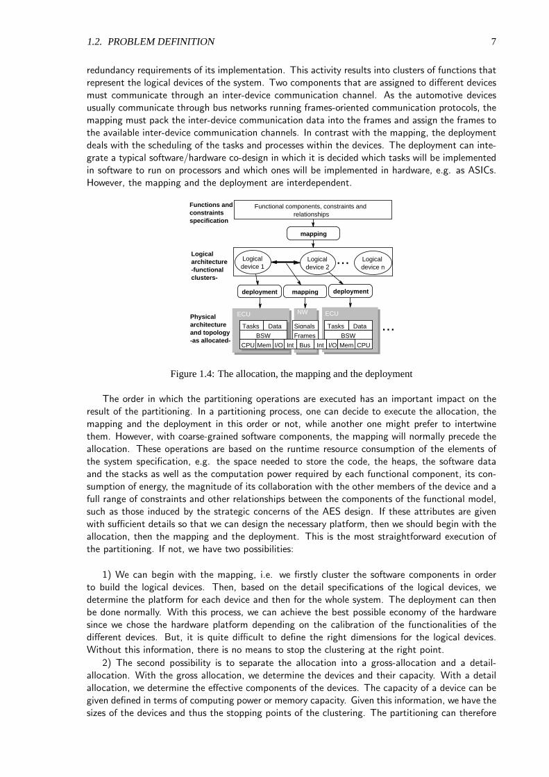
1.2. PROBLEM DEFINITION 7
redundancy requirements of its implementation. This activity results into clusters of functions thatrepresent the logical devices of the system. Two components that are assigned to different devicesmust communicate through an inter-device communication channel. As the automotive devicesusually communicate through bus networks running frames-oriented communication protocols, themapping must pack the inter-device communication data into the frames and assign the frames tothe available inter-device communication channels. In contrast with the mapping, the deploymentdeals with the scheduling of the tasks and processes within the devices. The deployment can inte-grate a typical software/hardware co-design in which it is decided which tasks will be implementedin software to run on processors and which ones will be implemented in hardware, e.g. as ASICs.However, the mapping and the deployment are interdependent.
Functional components, constraints and relationships
Functions and constraints specification
Logical architecture -functional clusters-
Logical device 1
Logical device n
...
Physical architecture and topology -as allocated-
Tasks Data
BSW
CPU Mem I/O Int Bus Int I/O CPU
BSW
DataTasks
Mem
Signals
ECU ECUNW
Frames
deployment mapping deployment
mapping
Logical device 2
...
Figure 1.4: The allocation, the mapping and the deployment
The order in which the partitioning operations are executed has an important impact on theresult of the partitioning. In a partitioning process, one can decide to execute the allocation, themapping and the deployment in this order or not, while another one might prefer to intertwinethem. However, with coarse-grained software components, the mapping will normally precede theallocation. These operations are based on the runtime resource consumption of the elements ofthe system specification, e.g. the space needed to store the code, the heaps, the software dataand the stacks as well as the computation power required by each functional component, its con-sumption of energy, the magnitude of its collaboration with the other members of the device and afull range of constraints and other relationships between the components of the functional model,such as those induced by the strategic concerns of the AES design. If these attributes are givenwith sufficient details so that we can design the necessary platform, then we should begin with theallocation, then the mapping and the deployment. This is the most straightforward execution ofthe partitioning. If not, we have two possibilities:
1) We can begin with the mapping, i.e. we firstly cluster the software components in orderto build the logical devices. Then, based on the detail specifications of the logical devices, wedetermine the platform for each device and then for the whole system. The deployment can thenbe done normally. With this process, we can achieve the best possible economy of the hardwaresince we chose the hardware platform depending on the calibration of the functionalities of thedifferent devices. But, it is quite difficult to define the right dimensions for the logical devices.Without this information, there is no means to stop the clustering at the right point.
2) The second possibility is to separate the allocation into a gross-allocation and a detail-allocation. With the gross allocation, we determine the devices and their capacity. With a detailallocation, we determine the effective components of the devices. The capacity of a device can begiven defined in terms of computing power or memory capacity. Given this information, we have thesizes of the devices and thus the stopping points of the clustering. The partitioning can therefore

8 CHAPTER 1. GENERAL INTRODUCTION
begin with a gross-allocation, then the mapping, and with the result of these operations, we proceeda detail-allocation and then the deployment. This process is for example the solution if we havea stock of devices at our disposal. It might involve many loops of allocation, mapping, detail-mapping, deployment and evaluation, but it is the most realistic process since the partitioning isnormally given the functional specification of the AES under construction, and the system designersknow approximately the capacity of the available devices.
In this work, we refer to a partitioning process that follows the above second process, i.e. itfirstly executes the allocation, then the mapping and finally the deployment. Since we are concernedwith the design of the architecture of the system, the allocation is reduced to the determination ofthe number of devices (i.e. gross-allocation) while the internal equipment of the individual devicesand the corresponding deployment are partially under the responsibility of the components suppliers.Following this separation of duties, the most actual objective of the system architecture design isto minimize the inter-device communication. With frame-oriented communication protocols, thisobjective is to be achieved by reducing the number of frames used to exchange information throughthe buses. To do that, the mapping must assign the most heavily communicating componentsof the functional specification to the same device. However, reducing the number of frames isnot the unique optimization goal of the mapping. Within this design process, the mapping isheavily constrained by the allocation. The mapping must result in executable partitions, i.e. eachdevices’ functionality must be schedulable and respect the capacity of the corresponding device.Furthermore, each device functionality must use the hardware that is installed in the correspondingdevice optimally, with respect to the defined room that must be reserved for the possible futureextensions of the device functionality. The allocation depends on the working load of the system.We can only determine the equipments of the devices for a given working load if we can measurethe execution time, the size of the software code, the magnitude of the communication of thecomponents of the system’s functional specification, etc. This information can only be providedif the partitioning is given a consequent description of the behavior and the functioning of thesystem, what is not always the case. In fact, depending on the functions that are assigned toa device and the design constraints, an automotive device might be equipped with all kinds ofprocessing units (including ASICs, micro-controllers, DSPs, etc.) as well as all kinds of memoriesand several intra-device communication systems (e.g. SPI, I2C, etc). Figure 1.5 shows a possibleresult of the detailed deployment with an ECU for which the system partitioner only defined theapplication software and the communication matrix. For all these reasons, the scope of this workis limited to the mapping. In the remainder of this work, the partitioning will refer to the mappingwhenever there is no need for precision.
Funktions Tasks, Processes
HAL, OS, NW driver, Comm contoller, ...
Application SW
Basic SW
ECU SW
ECU
HW Patform
ECU SW
ECU CommunicationECU
Messages
Micro-Controller, DSP, ASIC, ASIP, FPGA, ...
ADC, Mux, ... DIO, I2C controller, ...
Processing Units
I/O devices
HW Platform
RAM, Flash, EEPROM, ...Memories
SPI, I2C, ...Buses
Figure 1.5: Detailed allocation and deployment
The design cost is also an important factor of the price of a vehicle. We will reduce the cost ofthe design if we provide efficient and CAD-supported techniques for the implementation of AES.In the current practice, the partitioning is done manually by highly experienced OEM designers,usually called system integrators. The partitioning is currently limited to the addition of the newsoftware components on the existing system without changing the precedent contents of the de-vices. When the existing devices are overloaded, the system architect generally decides to add

1.3. PROCEDURAL METHOD TO SOLVE THE PROBLEM 9
new devices to implement the new functionalities. This optimistic approach of the partitioning isjustified by the fact that the existing systems are well-functioning and reliable configurations withstable communication matrices. A new design of the system architecture is practically equivalentto a design from scratch, economically unsupportable in this industry where the competition isextremely hard. In fact, the AES domain is a fast-evolving engineering field where new featuresbecome rapidly customary. The time to market is vital for each OEM. However, the direct con-sequence of this practice of the partitioning is the difficulty to enhance the system’s functionality.This shortcoming is illustrated by the excessive number of buses and processors installed in thenew vehicles. Thereto, during the partitioning, a system architect must take hundreds of oftencontradictory and competitive constraints into account. Keeping this information for a long time inmind is not easy for a human intelligence. Furthermore, done per hand the partitioning is guided byvague estimations and is so poorly documented that it is difficult to add new functionalities into analready partitioned system, e.g. after delivery, without adding new hardware. A further importantdisadvantage of manual partitioning is the fact that it is not possible to examine a large number ofsystem architectures. The design space is reduced to the solutions that are familiar to the designerand those that are deemed by his feeling to be potential good solutions. In this context, new,innovative and revolutionary architectures cannot be realistically expected. A CAD-supported par-titioning will allow automotive systems architects, so-called systems integrators, to investigate newarchitectural options. Automated partitioning will be time-saving and produce well-documentedand good system architectures since much more solution alternatives can be consulted. If provided,this will be an effective contribution to the goal of optimizing the economy and the performanceof AES.
1.3 Procedural method to solve the problem
For the partitioning, the exploration of the design space allows designers to find optimal imple-mentations of the system specification by analyzing various alternatives of both the architecture ofthe system and the hardware platform. This requires powerful and complete models. The existingapproaches for the partitioning input very low-level, fine-granular specifications (e.g. logical andarithmetical operations or simple assignments) at the level of abstraction given for example by theprogramming languages like C, C++, assembler, Java and similar specification languages. Unfor-tunately, because of the complexity of the automotive electronics, this dimension of granularity isdifficult to achieve when following a system-oriented design scheme. System-oriented developmentrequires a global view of the system, resulting in the handling of very complex models. As a specialdomain of interest, important works have addressed the specification of AES, producing appre-ciable results. Near general-purpose embedded systems-qualified modeling tools (UML [39, 60],SDL [8], SysML [12],...), domain-specialized modeling languages have been proposed for the de-velopment of AES (e.g. EAST-EEA[40], AADL[16], AUTOSAR[22], etc.). But as these solutionswere mostly focused on the definition of modeling languages, neglecting the substance of modelingitself, i.e. its potential methodological support for the design process, it is necessary to examine ifAES specifications presented at this level of abstraction are apt to support the partitioning of thesystem.
This observation leads to the structuring of this work in two main parts. We first need to definethe input specification for the partitioning. This must be a model that fulfills the requirements ofthe partitioning. In this part of this work, we need to investigate the level of support that is providedto system architects by the existing AES modeling solutions with regard to the partitioning. Here,we concretely need to answer questions like:
• Which information is needed in a specification to support the partitioning?
• Which modeling features are needed to provide this information?
• Do the actual modeling techniques provide these features?

10 CHAPTER 1. GENERAL INTRODUCTION
• How capable are the modeling languages used?
We would appreciate if there is a modeling solution that fulfills our expectations. Else, wemust define a convenient input specification for the partitioning. In the second part of this work,we will design the partitioning algorithms that will find the optimal system architecture. The twoparts are described with more details in the following subsections.
Defining the input specification for the partitioning
The development of AES has incontestably experienced a great leap forward during the last decade.On the way toward its maturity, the AES design has adopted the model-driven development scheme.The purpose of model-driven system development is to use models to study the artifacts of a systembefore building it. Model-driven development offers an effective way to decrease the technical andfinancial risk of try and error and improves the savings of design time and system resources,etc. and improves the quality (reliability, soundness, performance, electromagnetic compatibility,etc.) of the system. Furthermore, model-driven development has the potentiality to boost theinnovation, afford collegiate work and simplify the product maintenance. All these concerns arequoted to be vital in the automobile industry. Unfortunately, the state of the art in modelingembedded systems in the context of the automotive engineering does not yet allow the designerto take the best possible advantages from model-based development. In fact, even if modelingis current practice for today’s automotive systems designers, models are still considered as simpledescription and communication media, although in the context of hard competition that rules theautomotive industry, modeling can unacceptably continue to be a task that unnecessarily consumestime instead of being helpful and easy.
Hence, even though models are abstractions of the reality, useful specifications must highlightthe system characteristics, motivate the design options and facilitate the design decisions. In brief,a model should bear all necessary information needed for the subsequent design operations, forexample the partitioning. AES modeling is concerned with the specification of the architectures,the communications, the behaviors, the constraints and the non-functional requirements of theautomotive-embedded software and its electronics as well as the process of the system developmentand the contained transitions. Architectural models include the description of the structure of thesystem and its topology while behavioral models describe the system’s operation. Transition modelsare needed to capture the evolution along the design process. Modeling the transitions includes forexample the description of the mappings as well as the rules governing the relations between theabstraction levels, the instantiations, the configurations and the deployment. However, the value ofa modeling solution that is eligible for the AES design depends not only on the way it handles theseartifacts but also on how it considers the modeling of the automotive-specific domains of interestsuch as hardware platforms, product lines, non-software components (e.g. driver’s interaction),and vehicles environment (e.g. the road). High resolution, clear encapsulation, execution andsynthesis tools are needed in both the high- and the low-level design, while clear modularity isessential in the higher levels of the design to support the partitioning.
We have evaluated the most common modeling tools that are usual in the automotive designon their ability to support the partitioning. We examined low-level languages, i.e. program-ming languages and hardware description languages (HDL), and high-level languages includinggeneral-purpose modeling languages (UML, SDL, SysML) and automotive domain-specific model-ing languages (EAST-ADL and AUTOSAR). Unsurprisingly, we found that when the design followsa top-down strategy, none of the above languages can be expressive enough to be used efficientlyfor all purposes along the design process, since each of them offers in reality only a limited set offeatures. Otherwise, we are not aware of the existence of an all-rounder general-purpose model-ing language. At each step of the development process, the most adequate language should beselected depending on the actual conceptual layer, the level of abstraction and the intended useof the model. Within a system-oriented design scheme following a top-down strategy, the designof AES begins with high levels of abstraction for which the modeling languages like UML, SDL,

1.3. PROCEDURAL METHOD TO SOLVE THE PROBLEM 11
SysML, EAST ADL or AUTOSAR are adequate. Although all these languages claim sufficientorientation to the implementation, they still remain very abstract and lack synthesis and executiontools. However, as domain-dedicated languages, EAST ADL, SysML and AUTOSAR provide themost convenient features and the best precision needed to model automotive AES at the highlevels of the design, but they remain very insufficient to support the automated partitioning of thesystem. Firstly, because they are not synthesizable. Secondly, the semantics of ports, interfacesand connectors are fuzzy.
As we are dealing with a domain where the partitioning shall be done on high-level models,a promising solution to the first drawback is to combine these languages with synthesizable lan-guages such as programming languages, HDLs, etc. Two questions arise here: How should thelanguages be combined? and What are the best combinations? These questions are not in thefocus of this work since even the best combination will not be the ultimate solution for supportingthe partitioning of system specifications at high level. However, if EAST ADL and AUTOSAR lan-guages are enhanced with the missing capabilities, i.e. precise computations and communicationmodeling tools, accurate time and data handling, etc. so that the QoS of the model elementscan be extracted and analyzed, then they will represent appreciable solutions to build partitioning-compliant models of AES. We defined a modeling solution, the FN-for functional network-, that isfit for a CAD-supported partitioning at high level by adding some rules to the concepts importedfrom EAST ADL and AUTOSAR. In addition to the partitioning-friendly features provided by theselanguages, i.e. components detachability, standardized interfaces, QoS modeling, the FN providesclear screening of the communication paths and tracing of the communication data.
Partitioning AES
With the FN, AES functional specifications are modeled in the form of separable building blocks,where each building block represents a functional component of the system. As the FN allowsto clearly identify the boundaries of each model element, it enables to move each componentof the system and assign it individually to a given device. Furthermore, due to the concepts ofports and interfaces, the communication data can be properly specified with the FN, at leaststatically. In fact, although the FN is sufficient to model the structure of the system, it is lackingthe appropriate concepts to describe the behavior of the system. Instead of fine-granular and high-resolution modeling solutions that are desirable for the allocation, the FN, like all the standardsolutions that are adequate for the system-level specification of AES, proposes high-level modelingtools like state machines or communication, interaction, sequence, data flow diagrams, etc. tospecify the behavior of the system. Because of the low resolution of these behavioral modelingtools, it is not possible to produce a system specification that can be used for a detailed systemallocation, and much less for the deployment. In fact, the allocation and the deployment rely on theQoS attributes of the model elements. These attributes include the runtime resource requirementsof the functional components, e.g. the code size, the execution time, the communication load,etc.
In order to specify the system behavior so that these attributes can be extracted, we needmore detail specifications. These can be provided only for a single component that is also not toocomplex if we do not want to face an order of explosion of the size of the specification that willlead to the loss of visibility and reduce the navigation within the specification. Note that this isthe main reason why the mapping precedes the deployment. After the mapping, we can producemanageable behavioral models for each device and use them for the detail allocation and thedeployment. Although this strategy gives rice to much more loops of allocation-mapping-allocation-deployment-evaluation-allocation-mapping-... than with a straightforward process, we adopted itbecause of the incapacity of the actual state-of-the-art in the modeling of automotive systems toprovide more detailed specifications of the behaviors at the high level of the design. However,even if the runtime resource requirements of the functional components cannot be predicted withthe FN, we can appropriately use the syntax of communication diagrams, sequence diagrams and

12 CHAPTER 1. GENERAL INTRODUCTION
timing diagrams to specify their communication at the level of abstraction that is inherent to anAES system-level, with a precision that can be sufficient to determine the quantity of the dataexchanged between two components, the frequency of the data exchange, the timing organizationof the communication and the constraints on the communication. This solution provides sufficientmeans to measure the closeness between the system’s functional components, essential to guidethe mapping. We sampled the information extracted from this solution in a Components DataFlow Machine, the CDFM.
The CDFM is a modeling format that enables the analysis and particularly the synthesis of thedata flow within the system’s specification. We solved the problem of defining the optimal partitionof the input functional specification of an AES using a combination of constructive and iterativepartitioning algorithms. A constructive algorithm was used to generate a partition that was refinediteratively. As the number of devices to be installed in the system to run the required functionalitywas not predefined, we designed a Quality Threshold (QT) partitioning algorithm to construct theinitial partitions. The threshold is given by the capacities of the allocated devices. The refinementof an initial partition is achieved by the means of a specific adaptation of the Kernighan & Linalgorithm [86] whereas the quality of the partitions is based on the execution of a bin packingalgorithm that realizes the multiplexing of the communication frames, i.e. a mapping of the inter-devices communication data on the communication channels of the inter-devices communicationnetwork.
1.4 Contributions
The goal of this thesis is to provide a design process and the partitioning algorithms that will enableto automatically determine the architectures of AES. In order to implement a CAD-supportedpartitioning tool for the system-level architectural design of AES, it is necessary to define adequateinput models, formalize the relationships between the different models and within the models,formalize the partitioning constraints, design the partitioning algorithms, optimize them, applythem on the inputs and evaluate the results of the partitioning. To achieve these goals, this thesisprovides a broad overview of the design concerns of AES. It begins with a clear definition of AESthat includes the identification of the relationships between automobiles, electronic and softwaresystems that outline the importance of the latter in vehicles. Then, a detailed presentation of thereasons that motivate the need of CAD-based partitioning tools gives rise to the current challengesidentified in the automotive industry. The solutions proposed from both the academia and theindustry to cope with these challenges are evaluated and commented. A partitioning method isprovided.
Thus, although this thesis focuses on the design of the architectures of AES, its most importanttechnical contributions include:
1. A valuable sample of background information relative to the constitution of AES and theirdevelopment. This includes a particularly profound review of the specification, the modelingand the architectural design issues of automobiles’ E/E systems and the related designprocesses as well as the documentation of the state-of-the-practice, the actual requirements,the actual and the feature challenges of the AES design.
2. The definition of a framework for the evaluation and the classification of the modelingsolutions that are used in the development of AES.
3. The definition of reference modeling solutions that are fit to support the automatic definitionof AES architectures. This contribution includes a revealing evaluation and a categorizationof the main modeling languages that are used in the AES design with regard to their abilityto support the implementation.
4. A study of the interdependencies between E/E design processes, E/E models, abstractionlevels and E/E design operations.

1.5. PUBLICATIONS 13
5. The definition of a novel, original modeling format for the synthesis of AES high-level specifi-cations. This format can also be used for validation purposes, e.g. for simulation, verificationor test.
6. The definition of a partitioning process that is adapted to AES high-level system specifi-cations. This contribution includes the formalization of complex closeness factors in thecontext of a CAD-supported design of AES architectures and the development of powerfulclustering and partitioning algorithms for the design of AES architectures.
7. The definition of the means for the evaluation of AES architectures and the related metrics.A correlated but also important contribution is the formalization of a frame multiplexingapproach for the packaging of signals within frames.
1.5 Publications
By now, we have published some results of this thesis in international conferences [81] and [85].Some others are actually submitted for publication [84], [83] and several papers are in preparation.However, the contents of each of these papers are presented in details in this document as describedin the following section. We resume our publications in relation with this thesis as follows.
• Partitioning Metrics for improved Performance and Economy of Distributed Embedded Sys-tems. A. Kebemou in IESS proceedings on IFIP TC10 Working Conference, pp 289-300,Aug. 15-17 2005.
• AutomotiveArchitect: A Partitioning-Centric Modeling and Architectural Design Environ-ment for Automotive E/E Systems. A. Kebemou and I. Schieferdecker in INFOS 2008 proc.of the 6th International Conference on Informatics and Systems, 27-28 March 2008, Cairo,Egypt.
• Evaluating Modeling Solutions on their Ability to Support the Partitioning of AutomotiveEmbedded Systems. A. Kebemou and I. Schieferdecker, International Conference on Em-bedded and Ubiquituous Computing, Taipei, Taiwan, 12.2007.
• A Model-Based Design Approach for the Partitioning of Automotive Embedded Systems. A.Kebemou and I. Schieferdecker in INFOS 2008 proc. of the 6th International Conference onInformatics and Systems, 27-28 March 2008, Cairo, Egypt.
• The Components Data Flow Machine: An Intermediate Modeling Format for the Design ofAutomotive E/E Systems Architectures. A. Kebemou and I. Schieferdecker in DIPES 2008proceedings on the IFIP Working Conference on Distributed and Parallel Embedded Systems,Milano, Italy, Sept. 7-10,2008
1.6 Scheduling of the thesis
As illustrated in figure 1.6, the rest of this thesis is organized as follows: We provide an illustrativedefinition of AES in the chapter 2. We begin with an outline of the relationships between AES andembedded systems. Then, based on an example of functional inter-actions in AES, we introducethe automotive communication systems and we discuss the purpose of the automotive connectivity.Chapter 3 gives an overview of the usual design methods of embedded systems and the relateddesign activities. Also in this chapter, we compare the sequential design method with the concurrentdesign method in order to provide a basis on which an efficient design process can be proposed forAES. This is done in chapter 4. The second part of this thesis is concerned with the purpose ofmodeling. To mark the beginning of this part, chapter 5 presents the state-of-the-art in modelingAES. In chapter 6, we evaluate the modeling solutions used in the AES design on their ability

14 CHAPTER 1. GENERAL INTRODUCTION
to support the partitioning. As these modeling solutions cannot provide the best support for thepartitioning, we define our modeling solutions for the desired inputs in chapter 7. Then, theCDFM, the modeling format for the corresponding synthesis models is defined in chapter 8. In thethird part of the thesis, we investigate the partitioning of CDFM models. As CDFM models areformalized as graphs, the first chapter of this part, i.e. chapter 9, gives an overview of the state-of-the-art in the partitioning, particularly the partitioning of graphs. Then our partitioning algorithmsare described in the chapters 10 and 11 and the results of their applications are summarized inchapter 12. A general conclusion, given in chapter 13 closes the thesis.
1 st Part: Backgroung Knowledge - Definition of the Domain
Chap 2-4
2 nd Part: Modeling - Overview, Evaluation, Definition of the Input Models
Chap 5-8
3 rd Part: The Partitioning - Definition of the Partitioning, Partitioning Algorithms
General Presentation: Introduction, Motivation, Problem Definition, Solution Approach, Contributions, Organization
Chap 1
Chap 9-11
Application and Conclusion: Application, Results, Summary and Outlook
Chap 12-13
Figure 1.6: Vertical logic of the thesis

Chapter 2
Automotive Embedded Systems
In this chapter, we present the relationships between automotive systems and embedded systems. AsAES (automotive embedded systems)1 will be the subject of investigation of this work, it is necessaryto define the term AES in a way that canalizes every imaginative representation of the discoursed item.We begin by defining the term embedded systems. Progressively, we show how AES are concerned withembedded systems and then following an example, we give a survey of the networking of embeddedsystems in today’s vehicles. We discuss the means by which interdependent automotive embeddedfunctions that are geographically separated communicate with each other.Then we give a brief surveyof the different communication protocols used in the automobile industry. The most famous of them,the CAN protocol, will be more extensively presented in the part of the workdealing with the problemresolution.
2.1 Automotive electronics
2.1.1 Embedded systems
Most of today’s life facilitating instruments embody a processing unit which undertakes the com-putation and control tasks needed to realize their functionalities. Telecommunication systems(e.g. mobile and fixed sets, routers, switchers, ...), household appliances, multimedia and medi-cal equipments, manufacturing facilities for the industry, transportation systems (aircrafts, trains,automobiles, ...), etc., embed such electronic-based components. The term embedded systemis used to designate a computer system that is not perceived as such. It is a computer systemwhich is integrated in a larger system that hides it from the user. Originally, embedded systemswere specialized on a predefined functionality and were not able to work independently from theirenvironment. They could only operate when triggered by another system, e.g. a sensor or the user.This conception of embedded systems refers to a piece of silicon implementing a given functional-ity. In the last decade, the technological evolution has afforded the emergence of electronic devicesthat integrate several functions. Embedded systems are no more restricted to single-function prod-ucts that are conceived for a fixed and predefined functionality. They are becoming very complexand they can no more be conceived to react exclusively to the inputs of other systems. Modernembedded systems are increasingly requested to control complex and heterogeneous systems. Forexample, a high-definition TV handset controller must incorporate control and signal processingfunctions, audio and video data processing features, wireless and wired communication modules,etc. Such an embedded system can contain very heterogeneous functional blocks including DSPs,ASICs, memories, converters, etc. and sometimes it even might integrate a whole system on asingle piece of silicon. The latter is referred to as a SoC (System-On-Chip).
As the emergence of billion-transistor chips is just around the corner, the next generationof SoCs will implement more complex functions. Actually, Network-On-Chips (NoCs) implement
1In this context, automotive embedded systems (AES) is synonymous with automotive E/E systems
15
16 CHAPTER 2. AUTOMOTIVE EMBEDDED SYSTEMS
switches, routers as well as different communication formats and protocols to connect SoCs on asingle chip. NoCs will enable the integration of an exceedingly large number of computational,logic, and storage blocks in a single chip. Embedded systems are mostly used in systems thatare typically mission-critical, but also most of the time safety- and business-critical. Therefore,embedded systems are expected to operate reliably and faultlessly. They generally underly very highperformance and cost requirements. Thereto, to cope with the actual changing world, embeddedsystems must be scalable and upgradeable. This is why they are more and more implemented insoftware.
2.1.2 Automotive and embedded systems
The automobile is originally a machine construction product. Until 1967, the engine ignition andthe lighting systems of personal vehicles were controlled exclusively by electrical circuits [24]. Theelectrical components were connected with their actuators and their consumers by means of dedi-cated peer-to-peer cables. With the electronic fuel injection controllers, the first microprocessor-based devices appeared in personal cars in the ’70s when the worldwide oil crisis boosted the needfor control devices to reduce the fuel-consumption. The subsequent introduction of the electroniccruise control, the central doors locking systems and the gear steering units marked the beginningof massive integration of electronic units in the automobile. Over the years, the technologicalevolution has turned the vehicles into high-tech systems. Although the first image of a car mightstill be that of a large piece of hardware, one must be aware that there are hundreds of computingsystems and millions of software code lines implemented in each modern vehicle. Today’s auto-mobiles are heavily equipped with computers and associated software to control everything fromthe engine to the brakes, the cruise and all kinds of new on-board navigation and communicationsystems.
Each electronic control unit (ECU) embeds one or more processing elements and memories, eachof which is either a general-purpose, an application-dedicated embedded system or a combinationof both. Figure 2.1 shows a layered architectural representation of an ECU. From the bottomupwards: The first layer contains the material components used in the ECU, e.g. the processingunits (e.g. DSP, MCU, ASIP, etc.), the IPs (e.g. ASIC, ASSP, FPGA, ...), the memories and thecommunication media (buses, cables). The MCAL (Micro Controller Abstraction Layer) containshardware-specific software components called drivers. A driver is a software component that enablesto interact with a hardware device. Possible contents of the MCAL include the MCU drivers, thememory drivers, the I/O drivers, the drivers for the communication controllers, etc. The HAL(Hardware Abstraction Layer) contains further hardware-closed software components that serveeither as pilots for the I/O devices and the memory devices or as interrupt and communicationmanagers. The layer with the operating system (OS) builds an abstraction layer between theapplication software and the hardware details. It provides the API services that are necessaryto access and manage the resources (i.e. hardware, drivers, pilots, service managers). The OSprovides the scheduling and the interrupt services, the resource/memory and tasks managementservices as well as the task intercommunication and synchronization solutions that are needed bythe application that runs on the ECU. In the realm of embedded systems, OS are generally requiredto be RTOS, i.e. they must provide deterministic timing behavior.
Automobile electronic devices (ECUs) are rarely stand-alone components. They must commu-nicate to fulfill their duties. To achieve efficient communication, automobile ECUs are networkedon different architectures (bus, ring, star, tree) running several communication protocols, e.g.CAN, MOST, LIN, FlexRay, etc. We identify the collectivity of such networks and the connectedelectronic devices as automotive embedded systems (AES). Automotive embedded systems thusconsist of sensors, control units, actuators and several communication networks. Sensors are usedto collect the information about the operational and environmental conditions of the vehicle, e.g.temperature, speed, lightness, etc. Most sensors in automotive systems are ”intelligent”, i.e. theyare able to transform the collected physical or chemical values into electrical values that can be
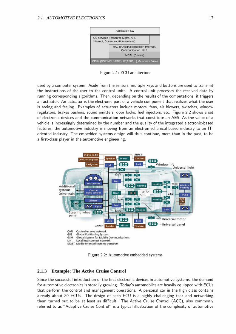
2.1. AUTOMOTIVE ELECTRONICS 17
Application SW
CPUs (DSP,MCU,ASIP), IP(ASIC,...),Memories,Buses
TextHAL (I/O signal controller, Interrupt, Communication, etc.)
MCAL (Drivers)
OS services (Resource Mgmt, API, Interrupt, Communication services)
Figure 2.1: ECU architecture
used by a computer system. Aside from the sensors, multiple keys and buttons are used to transmitthe instructions of the user to the control units. A control unit processes the received data byrunning corresponding algorithms. Then, depending on the results of the computations, it triggersan actuator. An actuator is the electronic part of a vehicle component that realizes what the useris seeing and feeling. Examples of actuators include motors, fans, air blowers, switches, windowregulators, brakes pushers, sound emitters, door locks, fuel injectors, etc. Figure 2.2 shows a setof electronic devices and the communication networks that constitute an AES. As the value of avehicle is increasingly determined by the number and the quality of the integrated electronic-basedfeatures, the automotive industry is moving from an electromechanical-based industry to an IT-oriented industry. The embedded systems design will thus continue, more than in the past, to bea first-class player in the automotive engineering.
Figure 2.2: Automotive embedded systems
2.1.3 Example: The Active Cruise Control
Since the successful introduction of the first electronic devices in automotive systems, the demandfor automotive electronics is steadily growing. Today’s automobiles are heavily equipped with ECUsthat perform the control and management operations. A personal car in the high class containsalready about 80 ECUs. The design of each ECU is a highly challenging task and networkingthem turned out to be at least as difficult. The Active Cruise Control (ACC), also commonlyreferred to as ”Adaptive Cruise Control” is a typical illustration of the complexity of automotive

18 CHAPTER 2. AUTOMOTIVE EMBEDDED SYSTEMS
electronic systems. The ACC is an enhanced version of the automatic speed limitation control,also called ”Tempomat” in some countries. In addition to the basic functions performed by theprevious automatic speed limiter, i.e. adjusting the car speed to a selected upper limit, the ACCprovides automatic collision detection and security distance adjustment. More succinctly, the ACCadjusts the vehicle’s speed to the changing flow of the surrounding traffic. It uses a three-beamradar sensor (see figure 2.3) to monitor the road in order to detect if an object moves ahead ofthe vehicle.
Figure 2.3: The ACC radar sensor
When the radar eye of the ACC detects an object ahead of the vehicle, the sensors pick upthe information concerning the location (e.g. the relative distance), the relative speed and otherattributes describing the movement (e.g. angle) of the moving obstacle. Based on this information,the ACC’s electronics determine if the object moves, and if so, the ACC will check if the objectmoves in the vehicle’s lane, then it immediately decides whether the car’s speed needs to beadjusted or not. Depending on the situation, the ACC autonomously initiates the slowing down orthe acceleration of the car. This is done through the activation of special engine management andbrakes activation functions. Moreover, when driving downhill, the ACC can automatically adjustthe car’s speed to the pitch gradient. The ACC is also able to recognize when the vehicle entersa curve. In this case, the ACC is able to adjust the speed of the vehicle to the accuracy of thecoming bend. If a car is moving ahead of the vehicle in the curve, the ACC will additionally takecare to keep a minimum (security) distance between the vehicle and the preceding car.
Further advanced features of the ACC include the driver support and the comfort. For example,the speed adaption when driving downhill or in curves is not only a security remedial action, butit is also a passengers comfort feature. In every critical phase of the traffic, the correspondinginformation (current status of the traffic, driving instructions, etc.) is displayed to support thedriver. For example, when a moving obstacle is detected in the vehicle’s lane, the ACC willautonomously display advising information at the same time as it starts the procedure that adjuststhe speed of the vehicle to the actual situation of the traffic. As soon as the obstacle is out ofthe lane, the ACC releases and the vehicle’s speed goes back to the control of the driver, withrespect to the chosen maximal speed if any has been set. Thereby, the setting of the ACC ismade comfortable for the driver as the ACC settings (selection of maximal speed, minimal securitydistance) can be done through all kinds of switches, steering arms or buttons from the dashboard.Figure 2.4 shows the electronic control unit running the main of the functionality of the ACC.
Figure 2.4: The ACC device

2.2. AUTOMOTIVE CONNECTIVITY 19
2.1.4 The ACC functional connectivity
The above description of the functioning of the ACC shows that the ACC needs to run functionsthat are located on different devices. Moreover, in addition to the data supplied by its sensors,the so-called ACC device needs information from other parts of the system. For example, the ACCcombines the data supplied by its sensors (e.g. relative distance of the obstacle, relative speed,etc.) with the car’s current course attributes (e.g. wheel revolutions, vehicle pitch, centrifugalforces acting on the vehicle, etc.) to calculate the tightness of the approaching curve and toadjust the car’s speed to maintain the necessary security distance. In fact, the ACC collects datafrom the accelerator pedal sensor, from the brake pedal sensor, from the setting buttons of theinstrumentation and the steering block, etc. The ACC also needs to activate some functions thatare located on different ECUs, e.g. braking functions, accelerators, lighting signals senders, etc.This necessitates the communication with the other devices.
Figure 2.5 illustrates the level of interconnection needs for the functioning of the ACC. The ACCis linked to the braking system, the stability control, the lighting system, the engine management,the dashboard, the steering control and the gears control, so that it can access data that isnecessary for its computations and can automatically activate the brakes, adjust the gear, displayinformation, instruct the fuel injection and the lighting announcements, etc. The functioning ofsuch a distributed application is highly dependent on the communication, the coordination andthe synchronization of different functions across the whole system and the real-time constraintsthat apply to the various functions performing the distributed functionality are determinant forits successful working, and thus for its acceptance. If the system does not react on time, itis useless and dangerous. If the system is informed on a critical situation too late or if thesystem’s instructions are received too late, the vehicle will probably not react as expected. However,in addition to the need of predictable behavior, automotive electronic-actuated features underlystringent costs constraints that depend on both their resources and the design time.
ACC
Gear ControlDashboardLight Modul
Steering Block
Stability Control
Engine Management
Braking System
Figure 2.5: ACC interconnection
2.2 Automotive connectivity
2.2.1 Automotive communication protocols
Several network technologies have been defined to cope with the particular requirements of AES.The transmission rate, the bandwidth, the real-time performance, the immunity against noise, thescalability, and the implementation costs are the most decisive attributes of these solutions. Asthe different networks are based on different technologies, they also present different interfaces,i.e. the word length, the header format, the physical medium, the bit rate, etc. according tothe networking solution. Gateways are used to interconnect the networks (see figure 1.1). Fol-lowing, we survey the most popular communication protocols that are used to interconnect theautomotive devices. The survey includes automotive domain-specific communication protocols,general-purpose protocols that have been implemented in vehicles or are identified as competitorsfor some automotive-specific protocols and the communication protocols that appear as trends for
20 CHAPTER 2. AUTOMOTIVE EMBEDDED SYSTEMS
future generations of vehicles. In order to be brief, we only pick out the principal characteristicsof these network technologies that can help us to understand their applications. For example,the medium access strategy and the arbitration method are important performance attributes thataddress the throughput, the transmission delays and the determinism of the network behavior. Thephysical medium has consequences on the weight, the shielding, the robustness, the price, etc. ofthe given network technology. The bandwidth and the triggering control of the network are alsoimportant indicators of its performance. The triggering control (event, time) indicates the abilityto react to asynchronous or synchronous events. Further important attributes, that are also usefulfor our understanding of the automotive networking include the size of the networks, the art ofaddressing, the handling of priorities and the jitter. The target application fields, the quality of theexisting implementations and the future (evolution) of the surveyed technologies will also improveour understanding of the criteria that guide the choice of the automotive designers.
2.2.2 All-rounder automotive communication protocols
Originally designed for automotive systems, some communication protocols have been adoptedin various domains such as in industrial production installations, home connectivity, etc. This isthe case with the CAN (Control Area Network) and the VAN (Vehicle Area Network). We alsoconsider the communication protocols such as the SAE J1567 and J1850 protocols, that originallyproprietary, where adopted automobile industry-wide.
The CAN (Control Area Network) [1, 2] is the most popular automotive communicationprotocol. CAN is used to network ”intelligent” devices (ECUs, sensors and actuators) within asystem. The CAN protocol was defined at Robert Bosch GmbH to enable automobile in-vehicleembedded communication. CAN has found wide application in the industrial automation, theaircraft and aerospace, the building automation (e.g. lift and escalators), etc. In automotivesystems, the CAN is generally implemented on a bus topology. CAN is an asynchronous, serialtransmission, multi-master and broadcasting communication system, using a CSMA/CA (CarrierSense Multiple Access with Collision Avoidance) media access method. That means that all CANnodes are able to transmit data and several CAN nodes can request the bus simultaneously. InCAN networks, data integrity[32] is assured by sophisticated error detection mechanisms and re-transmission of faulty frames. CAN is defined in the ISO standard ISO 11898-1. The protocolsupports single POF (Plastic Optical Fiber) or twisted pair cupric cables at the physical layer. Asingle cupric wire is allowed when the transfer rate is lower than 100 kbit/s. The bit rate dependson the bus length: short bus, high rate. The maximum specified transmission rate is 1 Mbit/s(in the high-speed version). This value applies to networks up to 40 m. For longer distances, thedata rate is reduced, for example for distances up to 500m a speed of 125 kbit/s is possible, fortransmissions over more than 1km the reasonable data rate is around 50 kbit/s. Theoretically, aCAN bus can support a non-limited number of nodes. But in the practice, an acceptable QoS isobtained by an average of 64 nodes.
CAN is an event-triggered bus concept, by which the frames are identified rather than thenodes. The identifier of a frame determines its content and also the priority that the frame enjoys incompetition for the bus access. Therefore, every frame identifier is unique within the whole system.The priorities of the frames are laid down off-line during the system design and cannot be changeddynamically. This concept allows the modular design of CAN networks, that facilitates the networkextendability. CAN networks offer high transmission reliability, but no deterministic frame latency.In the automobile industry, the high-speed CAN is usually implemented in vehicle’s chassis andpower train applications, on shielded wires in linear bus architectures. The main application domainof the single-wire CAN-bus is in the comfort electronic. As the CAN does not offer the degreeof real-time deterministic behavior that is necessary for safety-critical applications, it has beenenhanced to build a time-triggered variant, the TTCAN. However, the great success of CAN (i.e.CAN is implemented in most of the European cars and other high-volume markets like industrial

2.2. AUTOMOTIVE CONNECTIVITY 21
production controls, domestic and medical appliances, etc.) led to a low-cost implementation ofCAN devices and therefore guarantees the presence of the CAN in the future. CAN still has gooddays in the automotive engineering.
The SAE J1567 or C2d (Chrysler Collision Detection) protocol was defined by Chrysler as asensor network protocol with the goal to minimize the software overhead needed for the integrationof network nodes [79]. The C2d protocol prescribes a bus topology. The transmission medium isa twisted-pair of cables on which serial SCI-interfaces can be connected. The SAE J1567 protocolsupports a pulse width signal modulation and a multi-master media access (CSMA/CR) with abit-by-bit arbitration. The theoretical transmission rate is around 7.812 kbit/s. J1567 has beenimplemented by Chrysler for diagnosis and data sharing in the vehicle body, the chassis and thepower train, for example in the ”‘Grand Cherokee”’.
The SAE J1850 was seen in the last decade as the emerging standard for U.S. vehicles. J1850is designed as a combination of SAE J1567 with other proprietary protocols like the Ford’s HBCC(Hosted Bus Controller Chip) and the General Motor’s DLCS. It supports two multiplexing methods:a pulse width signal modulation (PWM) with a rate of 41.6 kbit/s and a variable pulse widthsignal modulation (VPWM) with 10.4 kbit/s. The transmission medium is a two-wire bus forthe PWM version and a single-wire bus for the VPWM version. J1850 is a CSMA/CR protocol,that means that there is no unique master on the bus. DaimlerChrysler, General Motors and Fordhave implemented the J1850 for diagnosis and power train services including engine management,transmission as well as the functions of the instrumentation and the ABS connections. But today,the SAE J1850 has been replaced by the CAN protocol.
2.2.3 High-speed and real-time protocols
To interconnect multimedia and safety-critical applications, the automotive engineering has de-signed high-speed and real-time communication protocols. Although the MOST (Media OrientedSystem Transport) protocol is actually the most famous protocol for multimedia applications, D2B(Domestic Data Bus), GigaStar, MML (Mobile Media Link) and other well-known general-purposecommunication protocols like FireWire/IEEE 1394 and USB are also serious candidates for multi-media applications. Moreover, a time-triggered version of the CAN, the TTCAN (Time-Triggeredon CAN), is competing with the other real-time protocols including TTP, FlexRay and Byteflightin the area of safety-critical applications.
A - Multimedia protocols
Most modern vehicles offer entertainment for the passengers (TV, movies, etc.) as well as vocaland visual assistance for the driver (navigation, representation of the images from video cameras).These applications need a broadband communication with real-time performance. We presentonly the MOST protocol because of its extremly dominant position in the list of the automotivemultimedia-capable protocols.
The MOST (Media Oriented System Transport) protocol specification [11] is a standardof the MOST Cooperation, that actually comprises BMW, DaimlerChrysler, Harman/Becker andOASIS Silicon Systems. With a bandwidth of 25Mbit/s, the MOST can connect up to 64 nodesin every possible topology, using a POF (Plastic Optical Fiber) at the physical layer. This is aconsiderable advantage in terms of electromagnetic compatibility, cost and weight. It is thereforenot surprising to find MOST implementations in practically every actual car in which multimediadata must be transported. MOST is a peer-to-peer network protocol that can be configuredas single or multi-master network. The MOST specification defines a multiplexing method thatclearly distinguishes the time slots for (synchronous) data transfer from those that can be used for

22 CHAPTER 2. AUTOMOTIVE EMBEDDED SYSTEMS
asynchronous frames. With its 25Mbit/s, today’s MOST is apt to supply most multimedia servicesat a good quality level. Since the evolution in the multimedia application domain is related with themagnitude of the data to be handled and eventually to be transported, other high-speed protocolswith larger bandwidths like FireWire (400Mbit/s, 800Mbit/s and probably up to 3.2 Gbit/s) andUSB 2.0 are competing to replace the MOST in the cars of the future.
B - Safety-critical application-compliant protocols
Real-time and deterministic behavior are particularly important for safety-critical applications.TTP, Byteflight, FlexRay and TTCAN are automotive domain-specific protocols with these prop-erties.
The TTP (Time-Triggered Protocol) is known in the avionics and the railway (www.ttagroup.org).TTP is designed for stringent fault tolerant real-time distributed systems. It is said to ensure thatthere is no point of failure in the system. TTP is a TDMA protocol where the arbitration is doneonce at the initialization time. TTP can be found in two versions: The low-cost version TTP/Athat is classified following the SAE (Society of Automotive Engineers) taxonomy as a class A pro-tocol, is a master-slave UART-based protocol, used in the automobile industry for sub-networking,i.e. branching several sensors (cluster) to a single ECU that itself is related to a backbone bus.TTP/A applications are known in engine control and car body applications, as competitor of theLIN and the low-speed CAN protocols. The higher performance version, designed for safety-criticaland fault tolerant hard real-time applications is the standardized TTP/C[107]. TTP/C offers abandwidth of 25Mbit/s on a bus topology. Because of its hard real-time capacities, the TTP/C isproposed in the automobile industry as a competitor of the TTCAN, and moreover of the FlexRay,particularly for x-by-wire applications.
The TTCAN (Time-Triggered communication on CAN) is an extension of the CAN withthe time-triggered paradigm. The TTCAN[19] is defined as a higher layer protocol on top of thestandard CAN protocol’s physical layer. The goal of the TTCAN is to provide the determinismneeded in the design of hard real-time systems. This is achieved by avoiding the latency jitters forthe media access and ensuring deterministic communication patterns. The TTCAN provides themechanisms to schedule the frames in a time-triggered way as well as in an event-triggered way.The TTCAN bus arbitration relies on a special, hybrid TDMA method, where every node accessesthe medium at predefined time slots, depending on the priority of the frame it is sending (see ISO11898-4). In order to support time-triggering and to handle asynchronous frames conveniently, theTTCAN protocol allows the definition of tree different sorts of time windows: The preassigned timeslots, called exclusive time windows, support the time-sharing medium access. The arbitrating timewindows support the handling of asynchronous frames. A node must compete for an arbitratingtime window in the same way as in a CAN network to send asynchronous frames. The thirdclass of time windows, the free-time windows, serves for eventual extensions of the network. Afree-time window can be converted in exclusive windows for new nodes or in arbitrating windowsto extend the bandwidth. TTCAN is implemented in the power train, i.e. for engine management,transmission, chassis control applications, and in some security- and safety-oriented car bodyapplications that need deterministic communication behavior. Since TTCAN is well adapted forx-by-wire applications, its future is considered very hopeful. Indeed, the implementation costs aremuch lower than those of its competitor FlexRay.
The FlexRay protocol is defined by the FlexRay Consortium (BMW, Bosch, DaimlerChrysler,Freescale, General Motors, Philips and Volkswagen) to be a protocol combining the attributes of theByteflight and the TTP protocols, including fault tolerance, deterministic behavior, collision-freetransmission, guaranty frame latency, arbitration-free medium access, flexibility in both bandwidth

2.2. AUTOMOTIVE CONNECTIVITY 23
and system extension, functional scalability and on-board diagnosis, support of optical and electri-cal physical layers. Moreover, the FlexRay Consortium (www.flexray.com) is guided in its initiativeby the need to simplify the design and manufacturing of vehicles, master the cost of the automo-tive micro controllers and other electronic devices while simplifying the system scalability. FlexRayintends to be a low-cost communication system, not only because of low component and imple-mentation costs, but also because of its ability to provide system scalability and its energy-efficientbehavior. For example, FlexRay supports a wake-up/sleep functionality (via bus) that addressesthe power management needs. The FlexRay specification targets on power train, chassis and bodycontrol applications. The FlexRay protocol provides a combination of static and dynamic frametransmission, incorporating the advantages of familiar synchronous and asynchronous protocols.FlexRay can be configured as asynchronous (event-triggered), synchronous (time-triggered) or amix of both. The communication medium consists of a single POF or two cables that act as twobuses, each offering a bandwidth of 10Mbit/s. A FlexRay network can connect up to 64 nodes.FlexRay is designed to support bus, star and cluster star topologies in single as well as in dualchannel modes. Some FlexRay implementations have been tested in Mercedes and BMW cars.The first commercial productions with FlexRay were expected by the end of the year 2006.
Byteflight (www.byteflight.com) is a FTDMA (Flexible Time Division Media Access) in-carelectronic communication protocol defined by a consortium around BMW to provide a means forfault tolerant communication with deterministic behavior for safety-critical systems. The flexiblebandwidth management of Byteflight enables easy on-board diagnosis. Furthermore, Byteflightis defined to be collision-free and low-cost. Similar to the CAN, Byteflight uses a frame-orientedaddressing via the awarding of identifiers. Hard real-time signals (alarm, etc.) can be prioritized.The physical layer is generally implemented on a star topology of POF (Plastic Optical Fiber)supporting half-duplex communication by up to 10Mbit/s. But bus and cluster topologies arepossible. Since 2001, Byteflight is implemented in BMW’s cars for passive (e.g. air bags triggeringand crash sensing) and active safety functions (e.g. belt tensioner), and for the body applications.
2.2.4 General-purpose protocols
Because of its severe cost constraints, the automobile industry is constantly looking for cost-efficientcommunication facilities. Hence, asides from the automotive systems specific communicationprotocols, the automobile industry has adopted a full range of general-purpose communicationstandards that are common for example in the consumer and building automation. USB, Bluetooth,SPI and I2C are such cost-efficient general-purpose communication protocols used to connectautomotive devices.
USB: With a bandwidth of 480Mbit/s and its plug-and-play capacity, USB 2.0 (Universal SerialBus)[15] is well-adapted for audio and video data transfer between the car and external peripheraldevices. USB 1.1/2.0 [14] is currently used to connect portable devices, e.g. navigation systems,external memories, flash card readers, video cameras, MP3 players or CD-writers, etc. to thevehicle. From the 4-wire communication medium of the first versions, the USB has evolved tooffer wireless communication possibilities. Some car makers are actually trying to connect vehicle’sembedded multimedia devices with each other through USB networks. Profiting in addition fromits broad bandwidth, the USB is supposed to gain more place in the automotive engineering in thenear future.
Bluetooth: Bluetooth (www.bluetooth.com) is an open specification for short-range (10-100 me-ters) wireless networking at low cost providing instantaneous connections between Bluetooth-enabled devices. Potential usage of Bluetooth in the automotive domain includes the wirelessconnection of mobile phones, portable DVD/CD drives or diagnostic equipments. Most automo-tive brands worldwide offer optional or standard Bluetooth-enabled communication systems in their

24 CHAPTER 2. AUTOMOTIVE EMBEDDED SYSTEMS
new models. Applications that enable hand-free usage in cars and synchronized operation of mo-bile phones with the car’s audio system are becoming popular. Unfortunately, although Bluetoothis a high-secured network (using authorization, authentication, FFH (Fast Frequency Hopping)mechanisms), we are yet not aware of commercial Bluetooth applications enabling vehicular ex-ternal connections, such as remote car handling. This is due to some deficiencies of the securityin the implementations of Bluetooth connections. In fact, the Bluetooth special interest groupfaces implementation weaknesses that can cause unsecured Bluetooth communications, such ascar whispering2, cabir3, bluesnarfing4, etc.
SPI: The SPI (Serial Peripheral Interface), a 4-wire serial communication interface that is oftenused by microprocessors to interface with peripheral smart chips in industrial and building instal-lations is a simple-to-implement synchronous serial protocol for connecting devices at low-speed(up to 5 Mbit/s). SPI connections follow a master/slave principle. Connected peripherals can beprocessors, converters (A/D and D/A), memories (EEPROM and flash), real-time clocks, sensors(temperature, pressure) or others (signal mixer, potentiometer, LCD controller, UART, CAN con-troller, USB controller, amplifier). When connecting two processors or two systems, the SPI canbe configured as a single-master-multi-slaves as well as a multi-masters-multi-slaves network withtwo control and two data lines. Since SPI lacks a standard specification, its implementations aredifferent from one chip to another, from one developer to another. SPI is used in the automobileindustry as a sub-bus (for smart networks). For example, SPI has been used to connect sensor’smicrochips in car’s instrumentations.
I2C: The I2C (Inter-IC bus) is like SPI also a control bus that provides communication linksbetween integrated circuits. I2C is a 2-wire serial bus standard (www.philips-semiconductors.com),supporting multi-master configuration, frame-priority and bi-directional communication from 100kbit/sin standard mode to 3,4 Mbit/s in high-speed mode. Only two lines (clock and data) are requiredfor full duplexed communication between multiple devices. The I2C protocol specifies a range of127 addresses. Each IC on the bus has a unique address. The I2C bus protocol allows collisiondetection, clock synchronization and hand-shaking features for multi-master systems. This simplebus concept is widely used for system control and data transfer from e.g. temperature sensors,voltage level translators, general-purpose I/O, A/D and D/A converters, CODECs, and micropro-cessors of all kinds. The automotive engineering uses I2C protocol for applications similar to thoseof the SPI application areas [7], i.e. for smart on-board networks.
2.2.5 Other in-vehicle and smart network protocols
LIN, ISO9141, K-Line, BSD, RS-232, RS-485, SAE J2058 protocols are implemented in secondaryin-vehicle networks (such as sensor networks subsidiary to a backbone net). The LIN protocolis (at least in Europe) almost the standard in this class, even if its specification itself is not yetstandardized.
LIN: The LIN (Local Interconnect Network) is defined to be a cost-saving (compared with CAN)protocol that can connect (intelligent) sensors and actuators through a single-wire medium [9].LIN communication is based on UART/SCI interfaces, very common and thus easily available atvery low price. LIN is particularly useful where the CAN is too powerful and too expensive, i.e. LIN
2The car whisperer is a software tool developed to enable the connection with the Bluetooth kit of a car in order tosend and receive audio and video data. Potentially, an individual using the tool can be remotely connected to a car andcommunicate with it from an unauthorized device, for example to send false audio information to the driver over the speakersof the car or the illegal visitor can spy the cars occupants by retrieving information from the car on its remote device
3The Cabir is a malicious software that when installed on a phone, uses Bluetooth technology to send itself to othersimilarly vulnerable devices. Due to this self-replicating behavior, it is classified as a worm.
4Bluesnarfing allows hackers to gain access to data stored on a Bluetooth-enabled device, e.g. phone, using Bluetoothwireless technology without alerting the user

2.3. CONCLUSION 25
is considered as a ”junior CAN”. It provides a 20kbit/s bandwidth for low-end applications. LIN’smain application field is in the car body, i.e. for applications like doors and sunroofs, servo steering,seats, climate regulation, lighting, mirrors, wipers control and similar applications. LIN networksare implemented in the vehicles of Smart, Mercedes, BMW, VW and a lot of other constructors.The size of a LIN network is typically under 12 nodes (actually 1..10). LIN guarantees a maximalframe latency. The LIN medium access is organized on a single-master arbitration. Each frame hasa unique identifier. The LIN master is charged to pilot the slaves (generally sensors and actuators),and at the same time it is the communication interface between the LIN (cluster) network andthe backbone network, e.g. CAN. Nodes can be added to the LIN network without requiringchanges in other slave nodes. Only the LIN master must be reconfigured when changes occur inthe network configuration. Recently, the LIN Consortium has published the version 2.0 [10] of theLIN that includes real-time capabilities, standard driver for all LIN-component hardware and thecertification of all LIN-components. This is an initiative to sustain the proliferation of off-the-shelfLIN slaves. When attached to a CAN backbone, the LIN network can access advanced systemdiagnostics services. As LIN has gained a wide acceptance, the LIN Consortium has good reasonsto project a positive future. The standardization of the functionalities of common LIN-slaves willaccelerate the vehicle design process, reduce the prices of the LIN-components and enable moreviable LIN-networks.
2.3 Conclusion
A premium-class vehicle today contains a considerable number of ECUs and some intelligent actua-tors and sensors (cf. figure 2.2) that need efficient communication facilities to provide the requiredfunctionalities. Currently, most of the communication protocols used in the automobile industryare either standardized or in a standardization process. Standardized communication protocolsafford modularity, distributed development, portability, external integration, cost reduction andachieve easy gateway functionality. CAN is the most used network technology in the automotiveengineering. A vehicle generally contains several CAN networks, each of them tailored for a partic-ular application domain (see example 1.1. Running at less than 125kbit/s, the low-speed CAN isusually implemented in the car body to network the devices that are concerned with the realizationof personal comfort, e.g. seats, doors, sunroofs and windows control. The air conditioning, the in-ternal lighting system, etc. are usually also controlled through a low-speed CAN network. A higherspeed CAN, that can runs theoretically 1Mbit/s, but generally operates at about 500kbit/s is usedfor more safety-critical functions like engine and gearbox control, brake and cruise management,etc.
MOST, USB and Bluetooth are promising solutions in the networking of automotive multimediaand telematics solutions, whereas FlexRay is observed as the future standard for hard real-timeand broadband applications and LIN for less constrained communications. As automotive-specifictechnology, LIN might remain for a long time the standard in the field of sensors and smart networks.TTP yields very good performance, but provides very limited means to treat asynchroneous andeven-triggered frames. In the same class with TTP and FlexRay, TTCAN is featured to managetime- and event-triggered frames, but its bandwidth is right limited. A pertinent observation showsthat TTCAN and TTP do either not seem to be well-prepared for the competition against FlexRay.
The panoramic view on the automotive communication technologies shown in table 2.6 refersto the most implemented protocols in the automobile industry from the OEM point of view. Theinformation (e.g. topology, implementation) given in this table is based on the implementationsof the protocols with regard to the automotive domain. The medium load represents the maximaleffective throughput, given as a percentage of the theoretical bandwidth. The maximum numberof nodes is the largest size with which the network is able to work with guaranty QoS. The costis coded as follows: 1 = very low cost, i.e. 0.5-2¤; 2 = low cost, i.e. 1-3¤; 3 = high cost, i.e.3-4¤; 4 = very high cost, i.e. > 4¤.
Although these automotive networking technologies are powerful, they are naturally limited.

26 CHAPTER 2. AUTOMOTIVE EMBEDDED SYSTEMS
Properties CAN TTCAN LIN Byteflight MOST FlexRay
Bandwidthin bit/s
Triggering
Medium(Length in m)
Latency
Topology
Medium
Load in %
Main
Application
Domain
Max Nbr
of Nodes
33,3k-500k…1M
20k 10M 25M 10M
EventTime
+ EventEvent Event/Time Event Time
Twisted-Pair/Single wire(40-1000)
SingleWire(40)
POF POF POF/Dual Cable
Variable Deterministic Deterministic Deterministic Variable
Bus Bus Bus Bus, Star Ring, Star Bus (12), Star(24)
50 ???50 60 15 90
32 (single wire)
110 Pair
32/110 12 22 64 64
PT, Body PT
X-by-Wire
SmartSubsystemsCluster NW
Comfort
BodyPassive
+ActiveSecurity
Multimedia
33,3k-500k…1M
TTP/C
Cost
(1,2,3,4)2-3 3
Twisted-Pair/Single wire(40-1000)
1 2 4
25M
Time
Deterministic
Bus
80
64
PTX-by-Wire
3
Twin axe Cable
PTX-by-Wire
Deterministic
???
Figure 2.6: Some automotive in-vehicle communication technologies
For illustration, the CAN, specified to run 1Mbit/s can only achieve a maximum of 500kbit/s inautomotive environments, due to the electromagnetic radiation on the twisted pair cables (shieldingis too expensive). The ideal communication technology for the automotive industry does actuallynot exist. Progress in the automotive E/E-related technologies i.e. including electronics, embeddedsystems design, communication and telematic will enable the integration of more functions intothe vehicles. For instance, the next wave of new features in automobiles will include parking aid,electronic toll collection, collision warning, personal digital assistance, driver alertness monitoring,intelligent brakes, etc. and extend existing functions to more complicated functionalities, forexample the new ACC (Adaptive Cruise Control) that is announced by the main European and Asianbrands will enhance the actual version with preemptive collision detection. Thus, the automotiveengineering must look for methods to manage the system complexity. In our mind, we will be ableto solve this problem if we can control the growth of the number of the device and optimize theusage of the capacities of the buses and the processors. It is thus well-advised to start today tolook for the solutions before the knock-out arises.

Chapter 3
Embedded systems design
The design of embedded systems is concerned with the development of the software and the hardware.The software is the program code of the system functionality. The hardwareis the material part of thesystem. As embedded systems constraints include the performance, the cost and the time-to-market,only proved and efficient design techniques are adopted. In this chapter, we give a survey of the embed-ded systems design methods that will help us to identify the similarities with the design of AES. Sincethe sequential design process does not allow the trade-offs and the efficiency that are so important inthe embedded systems design, we particularly focus on the concurrent design method.
3.1 Embedded systems design methods
3.1.1 The sequential design process
The most important activities in the embedded systems design include the specification of thesystem functionality, the conception of the hardware platform, the analysis and the implementationof the software and the hardware, and the integration of the software and the hardware. Thetraditional embedded systems design process makes use of a sequential design flow as shown infigure 3.1. Based on the specification of the system-desired functionality, the architecture of thehardware platform is decided. This activity is called allocation. Then the elements of the functionalspecification are assigned to the elements of the hardware platform. This is called binding ormapping. Afterward the application code is generated and loaded on the target hardware platform.This operation is the deployment.
Specification
HW Requirements Analysis
Conception of the HW Platform
SW Requirements Analysis
Development of the SW
Integration
Information flow
Process flow
Figure 3.1: Sequential embedded systems design method
The sequential development process can be roughly divided into two phases: The design of thefunctionality, the design of the hardware platform and the implementation. The implementationis concerned with the mapping, the development and the targeting of the code. The design ofthe hardware platform is guided by the type and the characteristics of the application. Based onthe characteristics of the application, the designer will decide which sorts of processors, memories,buses, interfaces, etc., must be used in the hardware platform. Depending on the calibration of thechosen components (e.g. clock frequency, memory architecture, levels of caches, communication
27

28 CHAPTER 3. EMBEDDED SYSTEMS DESIGN
protocols, synchronization techniques, number of I/O pins, etc.), the designer will decide whichnumber of each type of component is needed.
Typically, the allocation is not an automatic process. It is influenced by several unpredictablefactors like the availability of the components, the quality of the development environment of theexisting components, e.g. the quality of the coding tools (compilers, debuggers, simulators, etc.),as well as the preferences and the experience of the designer. In the implementation phase, thedesigner must try to take the best advantage of the processing power and the communicationbandwidth that is available on the platform, e.g. the tasks and the data of the application softwaremust be distributed optimally on the different components of the platform. This is achieved bythe means of the partitioning. The functional specification of the system has to be captured ina platform-compatible language. Depending on the hardware components on which the functionis mapped, the specification languages vary from ”high” level (e.g. Java, Pascal, Fortran, C)to ”low” level languages (assembler, bytecodes, ...). Note that the notion of ”high” and ”low”level languages is relative and absolutely contextual. With high level languages, i.e. as definedabove, an OS or a middleware is generally needed to link the application software on the hardwareplatform. The integration is concerned on the one hand with the deployment of the code on thehardware platform and on the other hand with the interconnection of the different components ofthe platform.
Following this development method, the platform is defined a priori, hopefully by ”gurus”,based on expert evaluation of the functionality and the constraints of the system. The imple-mentation of the system software is constrained by the chosen platform. The system partitioningis done after the allocation, whereas the designer supposes that the system will be successfullyimplemented on the available processors that are generally commercial-available processors. It isthus difficult to find the optimal tailoring for the hardware. Specific hardware is joined only whentiming or space constraints cannot be met. This is economically sensible, but in the embeddedsystems development, minimizing the price of the system is not the unique goal. The size, theweight and the power consumption of the system are often more important business criteria, forexample in the ubiquitous computing domain. In fact, a higher-sized hardware means more ma-terial, larger volume, supplementary weight and power consumption than needed, and thus highercosts. Furthermore, with this method, design errors such as the non-observation of the perfor-mance constraints are detected after the integration. This is obviously very late and changes inthe design may necessitate to reanalyze the specification. In the extreme case, the specificationmust be revised. The sequential design method can be a time-consuming, hazardous and thusan inefficient process with consequences on the time to market and the product cost. Variousalternative development flows have been proposed. Mostly differing only in the details. One of themost popular design methods proposes the concurrent design of the hardware and the software.This method is called HW/SW co-design.
3.1.2 The concurrent design method
The concurrent design of the different parts of a system is called co-design. In a co-design scheme,the functional specification is partitioned before the implementation begins (figure 3.2). Theco-designer supposes at the beginning that some parts of the system should be implemented inhardware to guarantee high performance and the rest in the software that will run on general-purpose processors, thus at low-cost. After the partitioning, the software and the hardware partsof the system are developed concurrently in observation of the communication interfaces betweenthem. Then, the hardware and the software are integrated and the whole system is validated withregard to its performance and its functionality requirements.
Compared with the sequential method, this design method allows to find better trade-offsbetween performance and cost. The co-design method allows to early detect incompatibilitiesbetween the hardware and the software. The communication interfaces between the softwareand the hardware can be easily optimized when these are designed cooperatively. The design
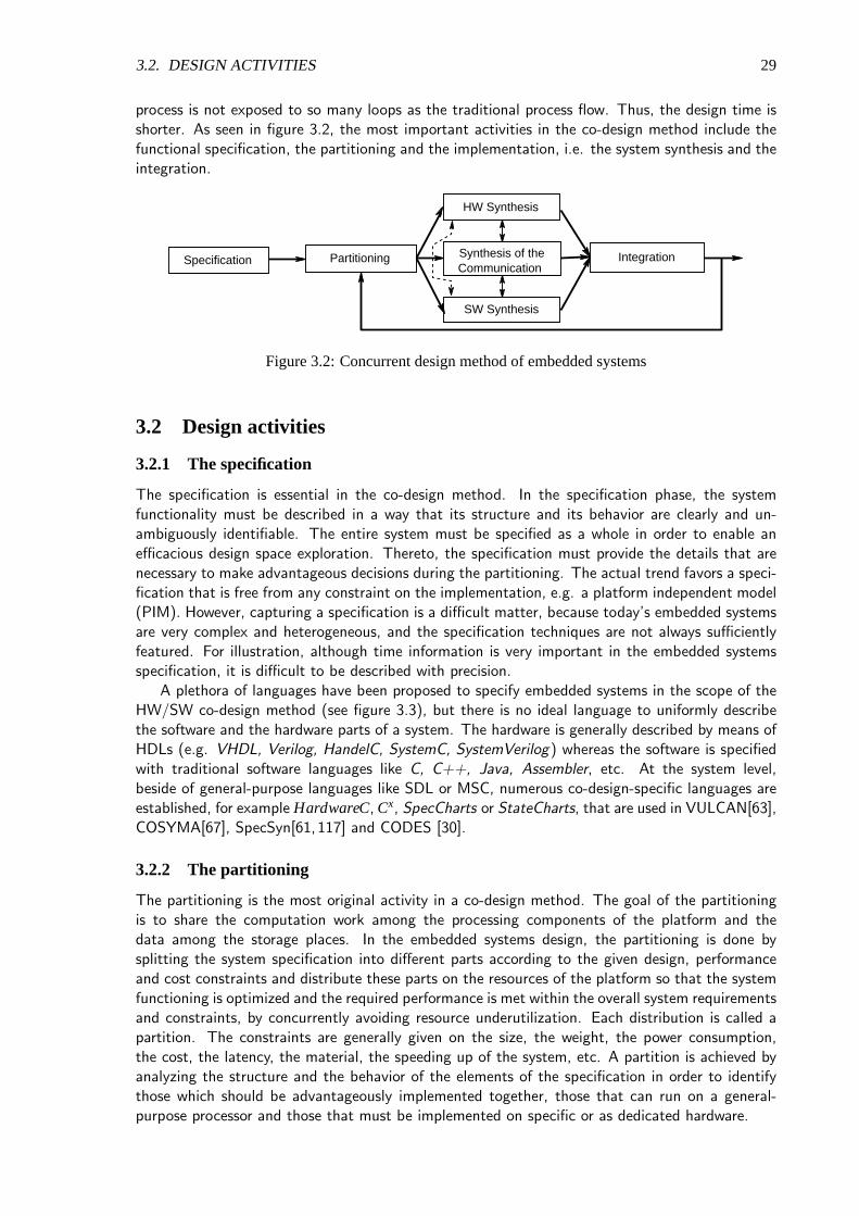
3.2. DESIGN ACTIVITIES 29
process is not exposed to so many loops as the traditional process flow. Thus, the design time isshorter. As seen in figure 3.2, the most important activities in the co-design method include thefunctional specification, the partitioning and the implementation, i.e. the system synthesis and theintegration.
Specification Partitioning
HW Synthesis
SW Synthesis
Synthesis of the Communication
Integration
Figure 3.2: Concurrent design method of embedded systems
3.2 Design activities
3.2.1 The specification
The specification is essential in the co-design method. In the specification phase, the systemfunctionality must be described in a way that its structure and its behavior are clearly and un-ambiguously identifiable. The entire system must be specified as a whole in order to enable anefficacious design space exploration. Thereto, the specification must provide the details that arenecessary to make advantageous decisions during the partitioning. The actual trend favors a speci-fication that is free from any constraint on the implementation, e.g. a platform independent model(PIM). However, capturing a specification is a difficult matter, because today’s embedded systemsare very complex and heterogeneous, and the specification techniques are not always sufficientlyfeatured. For illustration, although time information is very important in the embedded systemsspecification, it is difficult to be described with precision.
A plethora of languages have been proposed to specify embedded systems in the scope of theHW/SW co-design method (see figure 3.3), but there is no ideal language to uniformly describethe software and the hardware parts of a system. The hardware is generally described by means ofHDLs (e.g. VHDL, Verilog, HandelC, SystemC, SystemVerilog) whereas the software is specifiedwith traditional software languages like C, C++, Java, Assembler, etc. At the system level,beside of general-purpose languages like SDL or MSC, numerous co-design-specific languages areestablished, for example HardwareC, Cx, SpecCharts or StateCharts, that are used in VULCAN[63],COSYMA[67], SpecSyn[61,117] and CODES [30].
3.2.2 The partitioning
The partitioning is the most original activity in a co-design method. The goal of the partitioningis to share the computation work among the processing components of the platform and thedata among the storage places. In the embedded systems design, the partitioning is done bysplitting the system specification into different parts according to the given design, performanceand cost constraints and distribute these parts on the resources of the platform so that the systemfunctioning is optimized and the required performance is met within the overall system requirementsand constraints, by concurrently avoiding resource underutilization. Each distribution is called apartition. The constraints are generally given on the size, the weight, the power consumption,the cost, the latency, the material, the speeding up of the system, etc. A partition is achieved byanalyzing the structure and the behavior of the elements of the specification in order to identifythose which should be advantageously implemented together, those that can run on a general-purpose processor and those that must be implemented on specific or as dedicated hardware.

30 CHAPTER 3. EMBEDDED SYSTEMS DESIGN
Software Specification
Platform Architecture +Partitioning
Hardware Specification
NetlistSoftware Executable Code
HardwareC, SpecCharts, UML, StateCharts, SDL, Esterel, Signal, ...
C, C++, C#, Java,
Assembler, Pascal, Fortran,
...
VHDL, Verilog, System C,
SystemVerilog, ...
SW/HW Interface Specification
Validation
Performance Estimation
Prototyping
ASICProcessor
Interface
Evaluation
VHDL, Verilog,
System C, ...
Co-Validation
SW Synthesis SW Compilation
HW Synthesis
System Functional Specification +Constraints
Allocation +Mapping
Figure 3.3: Specification languages in the HW/SW co-design method
The partitioning process itself depends on its objectives. In some approaches, the partitioningaims at the definition of the parts of the system that will be implemented as hardware, i.e. customcomponent, and the parts that can be implemented as software to run on general-purpose pro-cessors. This is called HW/SW partitioning. The HW/SW partitioning is generally a functionalpartitioning, i.e. the functions of the system are grouped into consistent modules that are eachassigned to a platform component that is implemented either in hardware or in software. In an-other approach of the partitioning, the system specification is partitioned among several customcomponents, e.g. among several ASICs. This is a hardware partitioning. The hardware partitioningproduces an all-hardware solution since it does not consider any software component. Generally,in the hardware partitioning, the system is first implemented with (fine-grained) structural de-vices (e.g. gates), that are then partitioned among several custom components. This techniqueis called structural partitioning. The all-hardware implementation has the potential to providehigh-performance (via hardware speeds and parallel execution of operations) and reduced spaceoccupation, but is expensive in the fabrication of ASICs. The all-software implementation, evenwhen running on high-performance (general-purpose or specialized) processors is in principle thelow-cost solution, providing flexibility and upgrading, but it does not guarantee the achievement ofthe performance constraints and can incur high costs in developing and maintaining complex soft-ware. The trade-offs between quality, performance and cost are achieved through mixed HW/SWarchitectures, i.e. architectures containing general-purpose processors as well as custom processors.
3.3 The implementation
3.3.1 The software synthesis
The software synthesis is concerned with the implementation of the software part of the system,i.e. the embedded software, that will run on programmable hardware units and the configurationof the corresponding OS. This includes the translation of complex software descriptions (e.g.concurrency, timing behaviors or task scheduling) into a software language that can be compiledby common compilers, the coding, the targeting of the software and the optimization of the code,e.g. reduction of the amount of busy-waiting of the processor. This can be done automatically

3.3. THE IMPLEMENTATION 31
or manually. Because of its particular requirements, the embedded software development hasevolved to a special engineering field. In fact, the embedded software development is significantlyconstrained, not only because of the tight requirement on the code size, but also because of thelimitations concerning the implementation cost, the performance and the functional requirementsof embedded systems (dependability, maintainability, timeliness, concurrency, reliability, reactivity,real-time communication with the real world, etc.). For illustration, OS for embedded systemsare generally required to behave in real-time and concurrently, because of the shortage of space,embedded systems OS are tailored to provide only the minimum obligatory services. The principalactivities of the embedded software development are summarized in figure 3.4.
Specification
SchedulingChoice of the processors
SW and OS Implementation and Targeting
Validation
Figure 3.4: Design of the embedded software
Potential targets of the software include GPPs, DSP, MCUs and ASIPs. A GPP is designedindependently from any particular application, so that it can be used for a large set of applicationfamilies. Some examples are RISC, CISC, Sparc, Pentium processors. Nevertheless, some GPPsare optimized and thus specialized on a particular application domain (e.g. video, audio, mobiletelecommunication, etc.) but not on a specific application. Examples of domain-specific proces-sors include network processors, multimedia processors, Digital Signaling Processors (DSP), etc.DSPs are processors that are specialized on digital signal processing operations. Their architectureand their instruction sets are optimized for arithmetic operations such as Multiple-Accumulateoperations (MAC), pipelining, direct memory access, address coding and decoding, . . . that canadvantageously accelerate the operations that are usually implemented in signal processing algo-rithms, such as Fast Fourier Transform (FFT). DSPs are more powerful and space-saving thannon-specialized GPPs, but DSP development frameworks are generally tighter than those of non-specialized GPPs. For example, DSPs are generally more efficiently programmed in assembler thanin higher level languages like C. Microcontrollers architectures are optimized for control opera-tions. Their architectures and instruction sets are based on build-in clock operators and a largevariety of I/O devices, such as ADCs, timers, UARTs or specialized communications interfaceslike I2C, SPI or CAN. Microcontrollers have the advantage that they can be easily programmedwith high-level languages like BASIC. The range of utilization of application specific instructionset processors (ASIP) is tighter, since they are specialized on the common needs of a specific classof applications.
3.3.2 The hardware synthesis
The hardware synthesis aims at developing custom hardware, generally in form of ApplicationSpecific Integrated Circuits (ASIC). This activity is concerned with the process that transformsa description of the hardware part of the system in a description of the corresponding chips in aform from which integrated circuits can be manufactured. An ASIC is a processing unit that istailored for a task and only for this task. ASICs are very efficient in speed and resource usage, sinceonly the resources that are necessary for the application are effectively used. The ASIC solutionpromises the best economy of resources, space, weight and power consumption. But the lack offlexibility is dramatic with ASICs. Thereto, ASICs are very expensive in the manufacturing.
The hardware synthesis can be divided in two phases: The behavioral synthesis and the registertransfer-level (RTL) synthesis. The behavioral synthesis, also called the algorithmic synthesis inputs
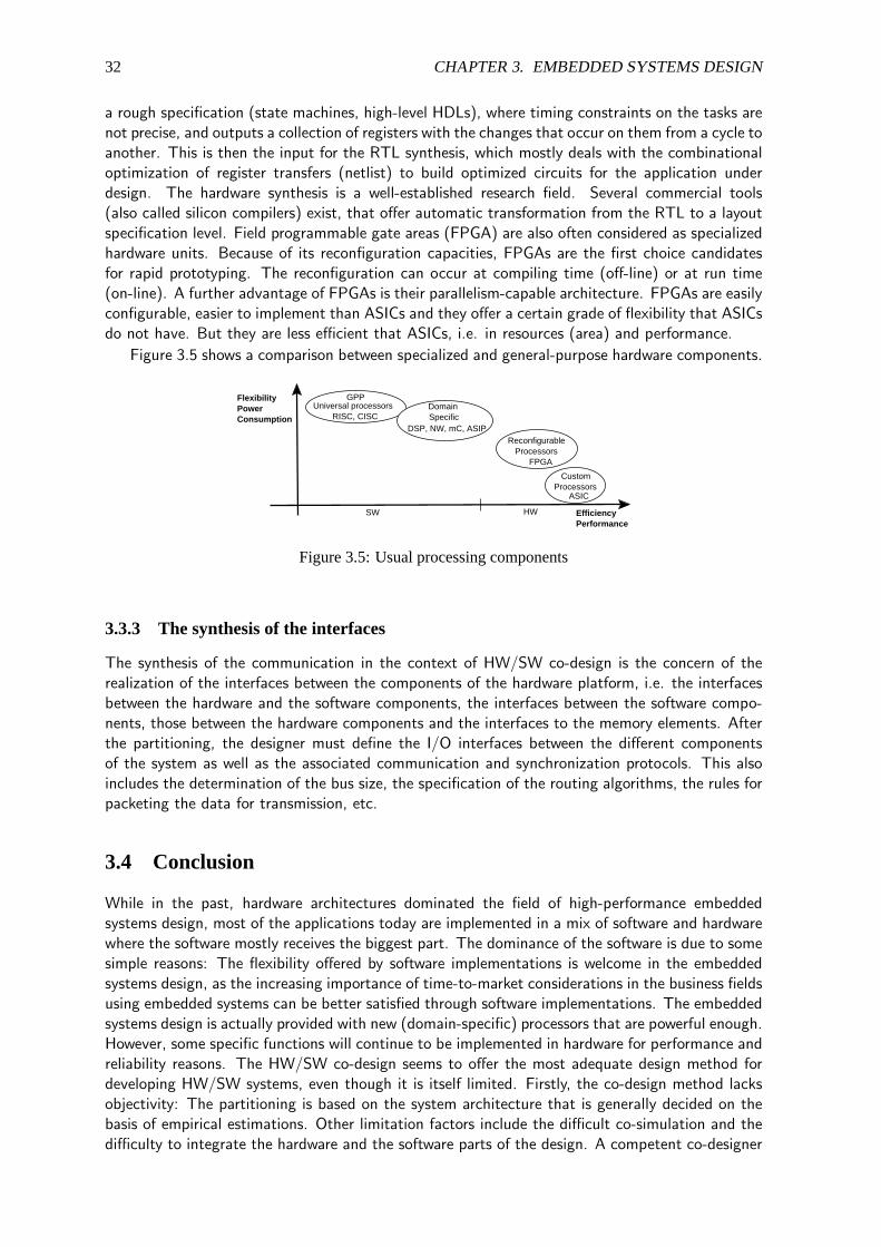
32 CHAPTER 3. EMBEDDED SYSTEMS DESIGN
a rough specification (state machines, high-level HDLs), where timing constraints on the tasks arenot precise, and outputs a collection of registers with the changes that occur on them from a cycle toanother. This is then the input for the RTL synthesis, which mostly deals with the combinationaloptimization of register transfers (netlist) to build optimized circuits for the application underdesign. The hardware synthesis is a well-established research field. Several commercial tools(also called silicon compilers) exist, that offer automatic transformation from the RTL to a layoutspecification level. Field programmable gate areas (FPGA) are also often considered as specializedhardware units. Because of its reconfiguration capacities, FPGAs are the first choice candidatesfor rapid prototyping. The reconfiguration can occur at compiling time (off-line) or at run time(on-line). A further advantage of FPGAs is their parallelism-capable architecture. FPGAs are easilyconfigurable, easier to implement than ASICs and they offer a certain grade of flexibility that ASICsdo not have. But they are less efficient that ASICs, i.e. in resources (area) and performance.
Figure 3.5 shows a comparison between specialized and general-purpose hardware components.
Efficiency Performance
Flexibility Power Consumption
HWSW
GPPUniversal processors
RISC, CISC
Reconfigurable Processors
FPGA
Custom Processors
ASIC
Domain Specific
ProcessorsDSP, NW, mC, ASIP
Figure 3.5: Usual processing components
3.3.3 The synthesis of the interfaces
The synthesis of the communication in the context of HW/SW co-design is the concern of therealization of the interfaces between the components of the hardware platform, i.e. the interfacesbetween the hardware and the software components, the interfaces between the software compo-nents, those between the hardware components and the interfaces to the memory elements. Afterthe partitioning, the designer must define the I/O interfaces between the different componentsof the system as well as the associated communication and synchronization protocols. This alsoincludes the determination of the bus size, the specification of the routing algorithms, the rules forpacketing the data for transmission, etc.
3.4 Conclusion
While in the past, hardware architectures dominated the field of high-performance embeddedsystems design, most of the applications today are implemented in a mix of software and hardwarewhere the software mostly receives the biggest part. The dominance of the software is due to somesimple reasons: The flexibility offered by software implementations is welcome in the embeddedsystems design, as the increasing importance of time-to-market considerations in the business fieldsusing embedded systems can be better satisfied through software implementations. The embeddedsystems design is actually provided with new (domain-specific) processors that are powerful enough.However, some specific functions will continue to be implemented in hardware for performance andreliability reasons. The HW/SW co-design seems to offer the most adequate design method fordeveloping HW/SW systems, even though it is itself limited. Firstly, the co-design method lacksobjectivity: The partitioning is based on the system architecture that is generally decided on thebasis of empirical estimations. Other limitation factors include the difficult co-simulation and thedifficulty to integrate the hardware and the software parts of the design. A competent co-designer

3.4. CONCLUSION 33
needs expertise in both hardware and software design, as well as in the design of communicationsystems.
Notable research have been done to help embedded systems designers and team managers tocope with today’s design requirements. ”High-level” specification languages have been developed,the partitioning can be automatized (at least partially), there exists a number of software andhardware synthesis solutions of performance. Some industrial tools that are available on themarket include: Arexys (SDL, VHDL, C), CoWare (C/C++), LavalLogic (Java to Verilog), Cynlib(C++ to Verilog), Art, Algorithm to RT (C++ to RTL), SUPERLOG (System-level descriptionlanguage). Known academical productions include: POLIS (U.C. Berkeley), PTOLEMY (U.C.Berkeley), VULCAN (Stanford Univ. (Hardware C)), CHINOOK (U. of Washington (VHDL)),COSYMA (U. of Braunschweig (C*)), MEIJE (INRIA and others (Esterel, Lustre, Signal)). But asembedded systems are becoming more and more complex, the level of granularity of the commonlyused specification languages in the co-design is too fine to capture large-scale systems. This isparticularly the case in the design of AES, the use of hierarchical specification techniques and aspecify-refine-verify loop design flow are necessary to cope with the actual complexity.

34 CHAPTER 3. EMBEDDED SYSTEMS DESIGN

Chapter 4
Automotive systems design
As a highly constrained domain of production, the automotive engineering needs efficient design meth-ods. In this chapter, we discuss the design of automotive electronics and we present the related prob-lems. In opposition to the actual components-oriented design process, we propose a more efficientdesign approach, based on the system-oriented perception of the design, that sketches and motivatesthe idea of co-designing the system’s devices. We define the problem to besolved and we precise thesolution strategy.
4.1 Design of AES
4.1.1 Top-down and bottom-up
The design of automotive systems can be divided in two views: The OEM’s view and the com-ponents supplier’s view. Figure 4.1 shows the interfaces between the OEM’s and the suppliers’sresponsibilities in the development chain of activities. The OEM is responsible for the whole ve-hicle. It is its role to define the functionalities of the system, and of course, it is the one thatorders the implementations of the corresponding functions. The components suppliers competeto acquire the implementation of the system’s components (i.e. in form of ECUs, software com-ponents or any other imaginable goods). The successful candidate must deliver the componentimplementation as specified by the OEM. After validation, the OEM integrates the componentinto the rest of the system and then validates all together, generally per test or simulation. Inmany automobile manufacturing companies, the development of the vehicle electronics is plannedfollowing some adapted versions of the waterfall model of development, i.e. an activity beginswhen the preceding activity is supposed to be finished. The relations between the phases of sucha development process can be easily represented in form of a V-model like in figure 4.1. This isa top-down design process (left side), completed with a bottom-up implementation process (rightside).
4.1.2 Current OEM design practice
Traditionally, the automotive industry sees the development of the electronic components (ECUs,actuators and sensors) like different activities that can be isolated and carried out independently. Inthe current practice, automotive electronic components are conceived like add-ons for the existingsystem. As shown in figure 4.2, ECUs and their software are each designed for a particulargiven functionality. Based on the requirements for the new features, a functional specificationis established, then partitioned to define the number of ECUs that should realize the neededfunctionalities. The OEM then orders the corresponding ECUs from the suppliers and plugs themon the system. After all, a range of tests is done to validate the integration. When the new featuresare proposed by a supplier, the OEM generally gets a black-box view of the new components thatare integrated and tested against their consistency with the rest of the system. This design method
35

36 CHAPTER 4. AUTOMOTIVE SYSTEMS DESIGN
System Level Design
Partial View Design
Components Design
Components Implementation
Partitional Level Integration&Validation
System Level Integration&Validation
Specification & Design Implementation & Integration
OEM
Components Suppliers
Components Definition
Components Level Integration&Validation
Global view System’s functional specifications: Logical & Technical Architectures
Domain restricted view Application domain specifications Logical & Technical Architectures
Component restricted view Components specifications: SW + HW Architectures
Partitioning
Development of SW + HW Components
Interface between OEM and Components suppliers
Ordering D
eliv
ery
Figure 4.1: OEM and suppliers views in the development process of AES
relies on a component-driven approach. The simplified representation of the development processshown in figure 4.2 makes abstraction of details that are not relevant for our purpose.
Existing SystemNew Features
proposed by a Supplier "as black box"
Requirements for new features "proposed by OEM"
Functional spec of the features
ECU’s interfaces & performance spec
Partitioning
Validation
Ordering ECUs
Integration & test
Interface spec and funtional description Interface spec of existing system
Figure 4.2: The components-based design process
4.1.3 Limitations of the current OEM design practice
In the design scheme described above, each ECU is designed for a fixed given functionality. TheOEM’s integrators are responsible to bring the different parts of the system together. They tryto make this easy by well defining the interfaces between the system’s components beforehand.This approach recalls the idea of modularity, well-known in the mechanical engineering, where theautomotive engineering, which is originally a machine construction industry, should have accu-mulated helpful experience. In fact, considering the complexity of automotive E/E systems, themodular design approach is absolutely right. But if the mechanical engineering can easily definestand-alone components, it is because these are essentially hardware pieces (metal, plastics, . . . ),which do not bear any internal live. The external behavior of these mechanical components is quasialways deterministic and thus, easily predictable. This is not the case for software and embeddedelectronic components. The clear link between structure and function that is typical to mechanicalobjects is not evident for intelligent systems. Furthermore, the interactions between the differentparts of intelligent systems seriously constrain their distribution. Here, modularity cannot encour-age careless separation of things that belong together. Unfortunately, automotive architects todaystill partition the specifications empirically, according to experience or vague estimations of theinter-components relationships. The consequences are obvious:

4.2. PROPOSED DESIGN APPROACH 37
• Too many ECUs
• High inter-ECU communication and underutilization of hardware resources, incuring poorcost/performance ratio
• The system integration is difficult and time-consuming
• The quality constraints (e.g. real-time requirements) are difficult to achieve at the sametime with the economy goals
• Difficult system scalability, since new functionalities are only introduced through the inte-gration of new ECUs
To solve these problems, the automotive industry designs more and more powerful communica-tion protocols, e.g. TTCAN, FlexRay, Byteflight, TTP, LIN, etc. If necessary, new buses, i.e. wiresare added to increase the communication bandwidth. Unfortunately, these solutions are not suffi-cient! Like the maximal load of the transmission medium, the performance of the communicationprotocols is limited. Adding buses implies to extend the cable harness, thus to increase the weight,the energy consumption, the product selling price and the technical problems (e.g. robustness).This development process is limited to manage the expansion of the current architecture and istherefore not apt to master the growing complexity.
4.2 Proposed design approach
4.2.1 Factors of the problem resolution
Nowadays, the differences between vehicle constructors in terms of manufacturing ability are prettyslim. The ability to design efficient, reliable and cost-optimal systems on time is essential to survive.In this context, the design flow can make a difference. Our aim is to master the galloping complexityof AES in such a way that avoids the explosion of the system cost by concurrently improving thesystem performance. AES costs are materialized by the vehicle selling prices and the costs ofownership. The vehicle selling price is based on the engineering costs (NRE) and the costs of thematerial installed in the system. We can control the costs of AES if we provide efficient designprocesses and innovative design techniques that can induce positive effects on the engineeringcosts and optimize the material usage. AES performance is measured on the real-time behavior ofthe computations in the system components and the timeliness of the communication. Each ECUuses a platform of processors (i.e. microcontrollers, ASICs, DSPs, etc.) and memories on whichthe associated application runs. We will optimize the costs of the material used in the system ifwe optimize the costs of the hardware in the ECUs and the cost of the communication system.The latter will be achieved by reducing the cable harness in the system while the former dependson the resource management techniques and the scheduling strategies applied in the ECUs.
In order to decrease the engineering costs and the costs of ownership of AES, a helpful designapproach must provide time-saving and flexible design processes. CAD-supported design opera-tions enable short design times and allow easier documentation of the design process. For theoptimization of the material usage, we need an efficient resource management that can:
• Reduce or at least slow down the galloping growth of the number of ECUs in the vehicles,
• Reduce the inter-ECU communication,
• Facilitate the system updating and upgrading and
• Simplify the system scalability so that OEM can sell software functionalities on demand,which can be flashed into a vehicle after delivery.

38 CHAPTER 4. AUTOMOTIVE SYSTEMS DESIGN
Suitably localized functions communicate cheaper and can easily share the resources. Thus, agoal-oriented approach of the partitioning, which can be automated is the key to master the costsand the performance requirements of the design of automotive electronic systems. Several factorsare needed to achieve these goals, for example we must be able to:
• assign functions to ECUs independently of the underlying hardware,
• define the ”occupation grade” (working load) of the hardware platform,
• provide efficient design processes with CAD-supported design operations.
4.2.2 The system-oriented design approach
In order to achieve our goal. we propose a system-oriented design approach, i.e. we perceive theelectronic system of a vehicle from the beginning as a ”whole”, joined mixture of hardware andsoftware components rather than a simple collection of parts. So, we can be constantly consciousof the dependencies between the parts of the system. We propose a partitioning approach thatcan be automated, and thus, enable CAD. The flow of the design as we conceive is sketched infigure 4.3.
System Spec
Logical Device 1
System Integration & Validation
……..Interface
Configuration
& Validation
………
System Requirements
Mapping
System Constraints Spec
ECU Allocation
Functional Spec for ECU 1
Logical Device 2 Logical Devices n
Deployment
SW Implementation HW Synthesis
ECU Integration & Validation
OEM
OEM or
Components
Supplier
Interface
Configuration
& Validation
Ordering Grey Box ECUs
RefinementRefinement
OEM
Assignment
System view
Components view
System view
Constraints
Constraints
Functional Spec for ECU 2 ………
Figure 4.3: System-oriented design approach
The specification: In a system-oriented design scheme, we shall separate the design of the ap-plication software from the basic software and the hardware platform, so that the design of theapplication software is free from the constraints of the hardware and the basic software and viceversa. This separation of concerns allows us to inventory and estimate distinguished design options.
The partitioning: The partitioning is done according to the performance and the cost objectivesin conformance with the system constraints. The mapping is the assignment of the elements ofthe functional specification to the components of the platform, i.e. the functional components areassigned to the devices and the inter-ECU communication data objects are grouped into the frames.The mapping must guarantee the consistencies (in terms of configurability and performance) of the

4.2. PROPOSED DESIGN APPROACH 39
interfaces between the function clusters. After the mapping, each ECU can be developed followinga typical co-design method.
The system integration: The OEM is responsible for the system architecture. It orders the devicesfrom component suppliers and integrates them together. Then, after successful tests, the systemis validated.
4.2.3 Analysis
The system-oriented method provides the ability to design more efficient systems, since each com-ponent of the system is designed as a part, rather than a stand-alone or a self-completing com-ponent. This process reveals several similarities with the concurrent design method of embeddedsystems as well as with the AUTOSAR design flow:
• The design starts with a system-level specification where the desired system functionality isspecified, analyzed and designed as a composite of building blocks,
• Like in the co-design, the partitioning aims at deciding which functions of the specificationwill be implemented together,
• The logical devices are analyzed, specified and refined concurrently,
• The allocation determines the number, the equipment of the ECUs, the topology of theplatform and the communication protocols for the inter-ECU communication, then
• The software/hardware partitioning, the scheduling of the tasks, etc. is done within eachdevice (the deployment) and
• The components of the system, i.e. the devices and the buses, are designed cooperativelyand implemented concurrently before being integrated and validated.
The AUTOSAR proposed design approach begins with a system-level functional description(figure 4.4(a)) where the system functions are encapsulated in AUTOSAR software componentsthat communicate through the VFB. This specification is then partitioned and mapped on thedifferent devices.
Figure 4.4: The AUTOSAR design approach (source: Autosar web content V23.4)
(a) The idea
ECU I
Virtual Functional Bus
AU
TO
SA
R
SW
-C
1
AU
TO
SA
R
SW
-C
2
AU
TO
SA
R
SW
-C
3
AU
TO
SA
R
SW
-C
n
...
ECU II
AU
TO
SA
R
SW
-C
1
AU
TO
SA
R
SW
-C
2
AU
TO
SA
R
SW
-C
3
ECU m
AU
TO
SA
R
SW
-C
n
RTE
Basic Software
RTE
Basic Software
RTE
Basic Software
...
VFB view
Mapping
System Contraint
DescriptionECU
Descriptions
Tool supporting deployment
of SW components
Gateway
SW-C
Description
SW-C
Description
SW-C
Description
SW-C
Description
(b) The activities
System Configuration
Inputs
System Configuration
System Configuration Description
ECU Specific Infos Extraction
ECU Specific Infos
ECU Configuration
ECU Configuration Description
ECU Synthesis and
Implementation
Appl. SWC, HW and Constraints Specifications
System configuration constaints
ECU Executable
Partitioning and Mapping infos Syst. topology, Bus mapping,
Appl. SW deployment Syst communication matrix
ECU architecture ECU SW, ECU HW and ECU
local Constraints Specifications
ECU Configuration Tasks scheduling, necessary
basis SW modules, configuration of basic SW, AUTOSAR Services, assigments of runnable entities to Tasks, Implementation technology
for each atomic SWC
ECU runnable SW ECU executables, code for RTE, basic SW(comm module, OS,...),
appl. SW and HWInput information flow
Process flow
Output information flow

40 CHAPTER 4. AUTOMOTIVE SYSTEMS DESIGN
The AUTOSAR design flow is roughly sketched in figure 4.4(b). The right-side items representthe design activities and their relationships. The left-side items are the products that result from thepreceding design activities. The products are given in the form of documents describing the resultsof the corresponding activity and the inputs for the following activity. The system configurationinputs include the software components, the allocated hardware and the system constraints. Thesystem configuration, i.e. the mapping of the software components on the devices and the mappingof the frames on the buses outputs the ”System Configuration Description” that contains allsignificant system information such as the topology, the bus mapping, the software componentsdeployment and the associated communication matrix. The system communication matrix is acomplete description of the frames (i.e. contents and timing behaviors of the frames) transportedaround the system. After the system configuration, the devices are configured individually, i.e.for each device, the runnable entities are assigned to the tasks, the tasks are scheduled, the basissoftware is defined and configured, etc. The result of these operation is described in an ”ECUConfiguration Description” from which the executables are generated. An ECU executable isthe code for the application software, the RTE and the basic software, plus the synthesis of thehardware components of the ECU if some do exist.
4.3 Conclusion
The components-oriented design approach of AES is obviously not capable enough to cope withthe problems following the explosion of the number of electronic-actuated features. The mostpromising solutions to these problems need a system-oriented approach of the design that enablesthe concurrent design of the components of the system. We propose a co-design approach thatmakes use of a partitioning of the system-level specification. However, this method will be realizableonly if the input specifications fulfill the requirements for the partitioning. Firstly, a system-oriented development method requires a global view of the system, resulting in the handling ofvery complex models. Thus complexity management and expressiveness are concurrently requiredfor the input specifications. Secondly, a qualified input specification must provide a certain degreeof freedom that is necessary to investigate various architectural alternatives. This necessitatesplatform independent functional specifications and configurable or standardized interfaces of thefunctional components.

Chapter 5
Modeling AES: State-of-the-art
In this chapter we overview the state-of-the-art in modeling AES. We first present the problematic ofthe modeling of AES, then we enumerate the features expected from an AES modeling solution. In thefollowing, we outline the techniques used to provide these features and we review the basic conceptsused to model AES in the actual state-of-the-art.
5.1 Modeling AES
5.1.1 Model-driven system development in the automotive engineering
The development of automobile E/E (Electric/Electronics) systems has incontestably experienceda great leap forward during the last decade. On the way to its maturity, the Automotive EmbeddedSystems (AES) design has adopted the model-based development scheme. The purpose of model-based system development is to use models to study the artifacts of a system before building it.Model-based development offers an effective way to decrease the technical and financial risk of ”tryand error” and improves the economy (design time, material usage, etc.) and the quality (reliability,soundness, performance, electromagnetic compatibility, etc.) of the system. Furthermore, model-based development has the potentiality to boost the innovation, afford collegiate work and simplifythe product maintenance. All these concerns are quoted to be vital in the automobile industry.Unfortunately, the state-of-the-art in modeling embedded systems in the context of the automotiveengineering does not yet allow the designer to take the best possible advantages from model-baseddevelopment. In fact, even if modeling is current practice for today’s automotive systems designers,models are still considered as simple description and communication media, although in the contextof hard competition that rules the automotive industry, modeling can unacceptably continue to bea task that unnecessarily consumes time instead of being helpful and easy.
The overall goal of modeling is to build the system. With a model-based design approach,models are expected to guide the whole design process. That means that all the activities withinthe life cycle of a car’s E/E system, from its conception to its destruction, must be supported bymodels as far as possible. Thus, here, models are the primary artifacts in the system developmentprocess. In our opinion, AES modeling must be outermost concerned with the support for theactivities of the implementation phase. Therefore, a model should bear all necessary informationneeded for the subsequent design operations. Hence, even though models are abstractions ofthe reality, useful specifications must highlight the system characteristics, motivate the designoptions and facilitate the design decisions. In the context of embedded systems design, one of themost decisive design operations is the partitioning, i.e. the assignment of the system specificationwithin the available resources. In the current practice, the partitioning is done inputing very low-level, fine-granular specifications (e.g. logical and arithmetical operations or simple assignments).Unfortunately, because of the complexity of AES, this dimension of granularity is difficult to achievewhen following a system-oriented design scheme. Coarse granularity is needed to describe suchcomplex systems, but coarse granular models are generally abstract. However, the quality of the
41
42 CHAPTER 5. MODELING AES: STATE-OF-THE-ART
partitioning depends on the information that is available in the input models. As a special domainof interest, important works have addressed the modeling of AES, producing appreciable results.Near general-purpose embedded systems-qualified tools (UML, MatLab, Simulink, SDL,...), moredomain-specific modeling languages have been proposed for the development of AES (e.g. EAST-EEA[40], AADL[16], AUTOSAR[22], etc.). But most of these solutions were focused on thedefinition of modeling languages, neglecting the substance of modeling itself and its potentialmethodological support for the design process. Some of these modeling solutions are nowadaysfirmly established in the AES design, but this engineering field is still seeking for a unified, consistentand robust modeling solution that will efficiently support the system development. This is partiallydue to the very particular nature of AES, i.e. AES are complex and highly heterogeneous.
5.1.2 AES are heterogeneous and complex systems
When considering a system-oriented design style, AES are very complex (in both the size and thefunctionality) and heterogeneous. In fact, AES are mixed compositions of hardware and softwaresystems that cooperate and also depend of each other. These aggregates are evidently different intheir natures and behave almost differently. As AES are multi-dimensional heterogeneous, the de-sign of AES must be able to manage different scales of heterogeneity. For example, even within thehardware and the software, there is a wide range of heterogeneous components, for example GPPand specialized processors, reactive and interactive tasks, event-driven and time-driven tasks, con-tinuous and discrete tasks, control-oriented and data/computation/transformation-oriented tasks,real-time and non-real-time tasks, etc. These items may necessitate different techniques of de-scription and design, but must be handled with the same care. In particular, the design of AESmust face the heterogeneity of the components, the heterogeneity of the specification languages,the heterogeneity of the abstraction levels.The heterogeneity of the components: The electronics of AES consist of ECUs and severalcommunication networks that are realized through cabled, optical or radio wave links running dif-ferent protocols. An ECU consists itself of hardware and software. Hardware components areof different sorts: GPPs, custom processors (ASICs, ASIPs, FPGAs, ...), memories, I/O devices,timers, etc.The heterogeneity of the specification languages: The heterogeneity of the components inAES indicates that it may be difficult to describe the whole system in a unique language. Eachpart of the system may be described using appropriate, e.g. domain-specific languages, resultingin a multiplicity of specification languages for the same system.The heterogeneity of the abstraction levels: The design process of AES is an agile cycle ofspecifications, validations and refinements that consequently involves different abstraction levelsinducing a vertical heterogeneity. Furthermore, when the elements that have been approved inprecedent designs are reused, the same abstraction level may contain objects that are in differentstages of development, i.e. in different levels of refinement. This fact yields what we call horizontalheterogeneity.
Hence, handling the complexity and the heterogeneity is a central issue in the AES design.
5.2 AES modeling needs
5.2.1 AES modeling prerequisites
Key prerequisite to manage the complexity and the heterogeneity is a clear separation of concerns.This is achieved through modularization and abstraction principles. Thereto, formal definitions ofthe modeling concepts would simplify the analysis, the validation and enable design automation.Modularization techniques allow to split the system into smaller parts that are easier to manage.Through this ”divide-and-rule” principle, AES are specified as networks of modules, each represent-ing a building block of the system. Usual abstraction techniques include the definition of different

5.2. AES MODELING NEEDS 43
views on the system under construction, the definition of different conceptual and abstractionlevels, the use of hierarchical decompositions, and the use of encapsulations. The definition ofdifferent conceptual levels of abstraction allows to write valid models with different degrees ofprecision. So, a specification can begin with non-mature but semantically correct models that willbe progressively refined as the design goes forth.
Encapsulation is a means for information hiding, domain delimitation and system isolation.Through encapsulations, the internal properties (structure and behavior) of a model element canbe hidden to the others. Encapsulations are necessary to isolate and protect one view fromanother one, one abstraction level from another one or one element of the specification (e.g.component, connection) from the rest of the specification. Encapsulation affords the detachabilityand subsequently the reuse of model elements. Anyway, despite the encapsulations, the relationsbetween the views and between the abstraction levels in the specification of a system must bemodeled to assure traceability. Traceability across the abstraction levels is modeled by meansof the refinement rules. Modularization and abstraction considerably afford the reuse of modelartifacts, the flexibility and the evolvability in the design process.
5.2.2 Features expected from an AES model-based design solution
AES system modeling is concerned with the specification of the architectures, the behaviors, theconstraints and non-functional requirements of the automotive embedded software and its elec-tronics as well as the transitions within the system development. An architectural model includesthe description of the structure of the system and the interactions between its components. Itmust support modularity, hierarchy and abstraction. Behavioral models describe the system’s op-eration, that is the ”sum” of the behaviors of the system components and their interconnections.The behavior of a component is made of two dimensions: The internal behavior and the externalbehavior. The internal behavior describes the part of the behavior that is concerned with the com-putations. The computations may be modeled using states transitions and flow graphs, activityschedules or algorithms. The external behavior describes the interactions of the component withits environment, i.e. the communication. Communication models involve the transfer of informa-tion between the communicating partners and the relationships (e.g. synchronization) betweenthem. Communication models are concerned with the description of the communication pathsbetween the system modules and the protocols that rule these communications. This may also in-clude further useful information like the scheduling of the communication, the access frequencies,the throughputs, the communication media and the information shared in the communication.Behavioral models must support the modeling of concurrency and time.
Constraints are statements that fix restrictions on the design. They restrain the design spaceand thus influence significantly the configuration and the implementation of the system. Usually,the constraints and non-functional requirements state obligations on the cost, the performance,the reliability, etc. Transition models are necessary for traceability of the evolution along the designprocess. Modeling the transitions includes the description of the mappings as well as the refinementrules relating the abstraction levels, the rules governing the instantiations, the configurationsand the deployments. This can be done by means of typical deployment and mapping/linkagedescription tools and some adaptations of feature trees. These points of interest can be placedin different views and treated at different abstraction levels. However, the value of a modelingsolution that is eligible for the AES design depends not only on the way it handles these artifactsbut also on how it considers the modeling of AES specific domains of interest such as hardwareplatforms, product lines, non-software components and vehicles environments.
A model-based design framework needs to:
• provide modeling concepts to capture these system artifacts,
• provide modeling languages to express the contents of the models,

44 CHAPTER 5. MODELING AES: STATE-OF-THE-ART
• define the design processes, i.e. the steps through which the creation of a system must go,their schedules and the corresponding activities and
• specify the design operations that are needed to perform the activities related to the processof system creation.
5.3 AES basic modeling concepts
5.3.1 Abstraction levels in the AES design
The cost requirements of automotive-embedded systems can only be met if portability and reuseare provided amongst others along the system life cycle. These aims can be achieved through con-ceptional separation of concerns. Model-Driven Architecture (MDA) proposes a two-layered designapproach consisting of platform-independent models (PIM) and platform-specific models (PSM).This approach allows long-term flexibility of the implementation and the integration. In the AESdesign, the system functionalities are specified as PIMs in so-called ”functional architectures (FA)”whereas the resources and the implementation details are handled in more ”technical architectures(TA)”, so that a FA can be deployed on a wide variety of platforms.
As shown in figure 5.1, the functional architectures focus on the design of the functionalities(functional views) of the system under construction. Typical models found in the FAs includethe structural models of product families and the corresponding behavioral models. The sys-tem behavior is typically specified with high-level logical information flow models (e.g. sequence,communication diagrams or state charts) or by means of algorithms. The technical architecturescontain the models describing the platform (hardware and basic software) on which the applicationwill run (i.e. infrastructural views). Depending on the abstraction level, the hardware platform canbe described in the form of a hardware abstraction (indicating which hardware device is installed inthe system but abstracting their real properties and locations) or at lower levels with its concretephysical elements (RAM, Flash, ROM, GPP, ASIC, bus, etc.). Typical models found in the TAsinclude the architectural models describing the platform components and their inter-connectionsas well as the topological models describing the positioning of the system components. The im-plementation level is concerned with the actual configuration of the system under construction. Itthus focuses on the refinement of the FA with regard to a specific platform. It uses architectural,behavioral and communication models to describe the system. Its primitives include software com-ponents and their inter-connections. The implementation models may also include the models todescribe the mapping, i.e. the assignment of its building blocks to the platform elements, and themodels to describe the allocation, i.e. the equipment of the platform. In contrast, the operationalmodels generally use primitives like processes, tasks and message frames as well as their dynamicaspects (tasks schedules, bus schedules) to describe the system.
In the ”EAST ADL” [40], the EAST-EEA has defined five conceptional levels: The vehicle level,the analysis level, the design level, the implementation level and the operational level, containingall together seven architectural models: The vehicle feature model (VFM), the functional analysisarchitecture (FAA), the functional design architecture (FDA), the logical architecture (LA), alsocalled function instance model, the operational architecture (OA) or allocation model, the technicalarchitecture (TA) or platform model and the hardware architecture (HA). These layers contain themodels that specify the system under construction in the intermediate steps of the design process,whereas each layer is a refinement of the preceding one. Following the same objectives, the authorsof ”AutoMoDe” [44] defined four methodological layers containing each one of the followingmodels: The FAA, the FDA, the LA and then the TA and the OA while the authors of ”AML”(Automotive Modeling Language) [45] defined four levels with the following models: The signals,the functions, the LA and the TA, completed with a special implementation level in which issueslike code generation and simulation are handled. The LA and the other conceptually closed modelsare concerned with the design of a particular product that is in general an instance of a family of

5.3. AES BASIC MODELING CONCEPTS 45
Requirements
Functional Models (Functions)
Constraints
Logical Architectures (SW Components)
Configurations
Mapping
Functions Cluster 1
Functions Cluster 2
Functions Cluster n
Deployment
Hardware Architectures
Refinements
Refinements
Refinements
Refinements
Functional Level
Implementation Level
Allocations
Platform and Operational Level
Figure 5.1: AES design conceptual levels
products. As the VFM, the FAA and the FDA are located in the methodological layers that areconceptually above the LA, they support the design of vehicle product families, i.e. product lines,variants and product configurations are modeled in these layers. Thus, the models of these layersdescribe the system functionalities independently of their integration in a particular product. TheVFM is intended to be a direct interpretation of the system functional requirements. Its componentsare the features that are expected from the system, such as anti-slip control, automatic gear controlor automatic lighting control. The FAAs and FDAs deal with the capturing, the structure of thefeatures of the VFM and their decomposition, while the OA is concerned with the deploymentof these functions on a given platform. These abstraction levels enable a methodological andconceptual separation of concerns so that the design process can easily begin with rough, abstractmodels that are progressively refined along the different levels. However, to design systems that arecomplex and highly constrained like AES, more specialized and methodological conceptual layersmight be necessary within the functional views, the implementation views and the infrastructuralviews (TA) to support the flexibility in the design process and enable methodical and evolutionarymodel refinements.
5.3.2 AES architectural modeling concepts
AES architectures are modeled as sets of communicating components, i.e. related modules. Asystem module is either an elementary (atomic) component or a composition (container) of othermodules. System modules interact by means of connections. A connection is an architecturalbuilding block that models the interactions between other building blocks and the rules that gov-ern these interactions. In some modeling techniques, connections are self-contained modules thatin addition to communication protocols incorporate computational behaviors, able for example totransform data or implement concurrency and synchrony mechanisms. Others define connectionsas simple transportation channels, that just need to have the right caliber to realize the commu-nication. However, accurate modeling of the communication (exchanged information, protocols,bandwidth, medium, etc.) is essential for the partitioning. A connection is realized by a set ofconnectors. Each connector may represent a channel in which the connected modules may sharesome information. A module is defined by its substance and its interfacing. In order to enablemodular development and reuse, modules are encapsulated. In this case, the interfacing capa-bilities of a module are specified by its encapsulation, i.e. encapsulations define the interfaces

46 CHAPTER 5. MODELING AES: STATE-OF-THE-ART
through which the building blocks communicate. An encapsulation is an architectural buildingblock that hides the proper characteristics of a module to the rest of the world. As the AES designis inevitably concerned with product lines, configuration and refinement rules are needed to assureclear transitions between the different methodological and conceptual layers. For illustration, aparticular system is built through configurations of some modules that have been defined as vari-ants in more abstract conceptual layers. Structural configurations describe the rules that governthe construction of valid architectures. For example, they determine if a module is appropriate fora particular product, which modules can be connected, if their interfaces match, if the connectorsenable proper communication and if a particular combination of modules results in the desiredbehavior. The refinement rules describe the rules that guide the transition from an abstractionlevel to another one. Generally, the functional behavioral modules of the system are identified asfunctions or (software) components and the links between them are simply seen as connectors.AES functional architectures designers usually do not care about data store modules. Also, inthis pragmatic way to simplify things, encapsulations are all supposed to be interfaces with ports[40, 44, 45] like those defined in the UML 2.0. Figure 5.2 shows a UML meta model representingthe AES architectures basic modeling concepts as they are generally implemented.
Functional Behavior
Data Store
1*
0..1
substance
Connector
Port
Variable Element
Module Connectioncontainer commmunicates
through *
Interface
*
*determines
*
11outin*
Figure 5.2: AES FAs basic modeling concepts
In contrast to functional architectures that are inherently logical, hardware architectures aredescribed with more physical objects. However, hardware architecture modeling concepts are quitesimilar to functional architecture modeling concepts. Figure 5.3 shows a meta model of AEShardware platform modeling semantics.
* srcPort dstPort *
ECU Sensor Actor Computing Elt Memory
container outInterface HW Port
HW Connection
in
Messages
send
NW Bus P2P
*
0..1
constituents
*
1
1..*
*
*receive
11..*has
1
Variable Element
HW Device
Figure 5.3: AES hardware platforms basic modeling concepts
In hardware architecture models, the basic module is the hardware device. Hardware portsare the points of interaction of hardware devices. A hardware device communicates with itsenvironment through its ports. Hardware ports may stand for fine-granular elements like pins ormore confederative entities representing a composition of pins, ports or other hardware devices.The communication is realized over hardware connections. A hardware connection is a hardwarearchitectural building block that models the communication between hardware devices. There aretwo families of hardware connections: Point-to-point connections and multi-point connections.

5.3. AES BASIC MODELING CONCEPTS 47
P2P connections model exclusive connections between two designated peer ports while multi-pointconnections model the communication buses. A bus may have several source and several destinationdevices. Thanks to the concepts of encapsulation (i.e. ports and interfaces), modules and hardwaredevices are detachable self-contained model elements that might be developed separately. Theseconcepts can be used at all possible abstraction levels. Concerning the partitioning, the qualityof an architectural model depends essentially on the grade of precision that is used to formulatethese concepts. For example, a hardware device is generally composed of other smaller devices,for example an ECU contains processors and memories while a memory is built up of registers, etc.Depending on the level of precision needed, a hardware device can be a transistor or the wholeplatform. Figure 5.4 shows some abstraction levels in the modeling of hardware devices.
HW Abstraction levels Primitives
System level
Register transfer level (RTL)
Logic level
Switch level
ICs level
Layout level
CPUs, ALUs, Memories
Registers, Macros (e.g. Adders, Subtracters, Multipliers, Buses, Multiplexers)
Gates, Logical operations (e.g. and, or, xor, not, ...), Counters,
Transistors
Resistors, Condensators
Polygons, BoxesSynthesis Analysis
ECUs, Sensors, Actuators, Networks, Processing Elements, Memories
Device level
Figure 5.4: Abstraction levels of the hardware devices
5.3.3 AES behavioral modeling concepts
The specification of the behavior of embedded systems is concerned with data transformation,i.e. the computations, and the communication of information. The AES communication schemestypically use a wide range of mechanisms, going from continuous to discrete time communications,synchronous and asynchronous, periodic, sporadic and aperiodic, and time- and event-triggeredcommunications. In the context of concurrency and resource competition between tasks that areomnipresent in embedded systems, synchronization and time paradigms must be supported by AESbehavior modeling solutions. Mode transitions, interactions-oriented models (e.g. sequence dia-grams), communication diagrams, flow-based models (e.g. data flow graphs, control flow graphs,control and data flow graphs) as well as all possible combinations of these tools have shownefficiency in modeling the behavior of embedded systems[41,44,74,118].
Special adaptations of states, activity, mode transitions, data and process flows have beenwidely used to capture the behaviors of embedded systems. State-oriented models have beenused in form of: Finite State Machines (FSM) [52], Extended FSMs, i.e. FSM extended withdata paths (FSMD) [51], FSM with Coprocessors Models, i.e FSMD considering architectureswith coprocessors (EFSM, FSMC) [68], Hierarchical Concurrent FSM (HCFSM) [27], CodesignFSM (CFSM) [93,94]. Examples of Petri nets based-representations of embedded systems includeTimed Petri Nets, Timed Place Transitions, Extended Timed Petri Nets (ETPN), Extended ETPN(PURE), Petri Nets-based Representation of Embedded Systems (PRES) [35, 36, 112, 119]. Butthe most straightforward approaches favor the common programming languages and other effectivetools such as Matlab/Simulink, etc. These techniques differently capture the characteristics ofembedded systems and therefore, they induce different levels of usage effort with different levelsof satisfaction.
48 CHAPTER 5. MODELING AES: STATE-OF-THE-ART
5.4 Conclusion
The AES design has adopted the model-based design scheme. The state-of-the-art in modelingAES relies on the components-based paradigm using generic concepts that can be easily adaptedto every abstraction and conceptual level. But, as long as these modeling solutions are abstractrepresentations of the system from which accurate information to support the design cannot beextracted, model-driven design will remain a dream. This dream will be realized only if we canachieve useful models at reasonable abstraction levels. In fact, the value of a modeling techniquedepends on the level of support that it provides for the intended operation. As we intend to partitionhigh-level specifications, it is important to evaluate the fitness, i.e. the level of satisfaction, providedby the available AES modeling techniques for the partitioning. This is the purpose of the followingchapter.

Chapter 6
The value of AES modeling languages
In this chapter we evaluate the capacity of the modeling solutions that address the AES domain re-garding their ability to support the partitioning. The overall goal of the evaluation is to identify amodeling language that can provide useful specifications for the partitioning. For instance, we needto answer questions like: Which information is needed in a specification to support the partitioning?Which modeling features are needed to provide this information? Do the actualmodeling techniquesprovide these features? How capable are the actual modeling languages?We first enumerate thefeatures that are expected from a model to support the partitioning and we define the framework forthe evaluation of the AES modeling solutions. Following this evaluation framework, the most commonmodeling languages used in the automotive domain are evaluated and classified.
6.1 The evaluation framework
6.1.1 AES modeling requirements for the partitioning
In the design of automotive E/E systems, one of the most decisive operations is the partitioning, i.e.the assignment of the system specification within the available resources. The exploration of thedesign space allows designers to find the optimal partitions of the system specification by analyzingvarious alternatives of both the partitioning and the hardware platform of the system. In a model-driven development scheme, design space exploration is enabled by powerful and expressive models.A pool of competing modeling solutions have been proposed to cope with the problems inducedby the growing complexity of automotive systems. As the principal features of these solutions areaxed around modularization and high level of abstraction, it is necessary to investigate their abilityto support the partitioning. An objective evaluation will be helpful to define how each modelingsolution should be enhanced for a better support of the partitioning, whenever necessary.
As AES are networks of sub-networks of ECUs, sensors and actuators, we identified two levelsfor the partitioning in chapter 1 (cf. figure 1.4). The second level of the partitioning, i.e. thedeployment, deals with the scheduling of the tasks and the processes on the processing units aswell as the scheduling, the synchronization of the communication and the data access proceedingswithin each device. Making these decisions requires sufficient information about the behavior, theresource consumption, the interdependences, the communication, the performance requirementsand the quality constraints of the elements of the functional specification. The first level of thepartitioning, i.e. the mapping, aims at distributing the system load among the devices in a mannerthat the system functioning is optimized by concurrently avoiding resource underutilization. Thus,during the mapping, the functional components of the system specification are distributed withinthe devices and the inter-device communication data is assignment to inter-device communicationchannels. The goal of the mapping is to find the most cost-sensitive feasible partition, i.e. apartition that optimizes the resource usage within the devices and minimizes the communicationload within the required performance and system constraints (e.g. flexibility, maintainability, powerconsumption, cost, safety, speeding up, etc.). A feasible partition is one that respects the intake
49

50 CHAPTER 6. THE VALUE OF AES MODELING LANGUAGES
capacity of the available devices. That is, it must respect the storage capacity of each allocateddevice, allow executable scheduling of the tasks and enable smooth inter-device communications.
In addition to the resource needs of the elements of the functional specification, the mappingrelies on the quality of the information about the inter-components communication, the degreeof freedom that is given to the designer and a wide range of relationships between the elementsof the functional model, such as those induced by the constraints and the strategic concerns ofthe design. For instance, the solution space of the mapping depends directly on the degree offreedom that is allowed both by the constraints and the strategical concerns of the design andby the proper definition of the elements of the functional model. The mapping requires that thesystem components must be each detachable from the rest of the system so that they can beindividually assigned to a device independently of the other components. A total freedom is thengiven for the mapping if each system functional component interfaces the others very loosely. Themapping of the communication data relies principally on the information about the timing behaviorof the communication and the magnitude of the communication between the system functionalcomponents. Timeliness is determined by attributes like the latency, the max activation time,the transmission time of the components, etc. The magnitude of the communication betweentwo components is given by the access frequencies and the dimensions of the communicateddata. To support the mapping, AES input specifications must thus enable to clearly identifythe boundaries and the interfaces between the components, identify the communication paths,extract the substance and the heaviness of the communications (e.g. throughputs, access rates,data resolutions, timeliness, priorities, security levels, etc.), find out the dependences and causalityrelations such as sequentiality, concurrency and the relationships resulting from the constraints andthe strategic concerns of the design.
6.1.2 Related work
The aim of the evaluation or the classification of modeling techniques is to measure and comparetheir potential level of support, their adequacy and their usefulness regarding the requirementsof the intended design activity, in our case the partitioning. During the partitioning, the systemarchitect will decide to assign each component of the system to a given part based on attributeslike its resource consumption, its size, its needs for computation power, its consumption of en-ergy, the magnitude of the collaboration with the other members of the part and a full range ofother significant dependencies. To enable the incorporation of the necessary information in themodels, a modeling technique must provide a certain level of precision for structuring paradigms,computation paradigms, control paradigms, communication paradigms and for the specification ofthe constraints and the non-functional requirements. In this context, precise information aboutthe boundaries and the substance of the system components, the competition for a resource, thetiming behavior of the model elements, etc. are very useful.
Several frameworks have been proposed for the evaluation and classification of embeddedsystems specification tools. The authors of [52] proposed a classification framework based onfive specification styles: State-oriented (using state machines), activity-oriented (using transfor-mations), structure-oriented (concentrating on structural architectures), data-oriented (based oninformation modeling) and heterogeneous. This classification is mainly based on syntactic criteria.However, it can be used to select a specification style depending on the nature of the behaviorthat needs to be captured. In contrast, the authors of [94] argue for a classification based on themodel of computation (MOC) of embedded systems languages. Using the Tagged-Signal Model(TSM) [96], a formalism for the description of MOCs aspects, they focus on timing, concurrencyand communication aspects to analyze and classify several MOCs. Generally, as the user is notaware of the MOC of a language, he will not be a priori aware of its quality also. It is thus difficultto apprehend the strength of a language based on its MOC. For instance, a good implementation(i.e. easy and clear syntax, powerful tool support) of a poor MOC is generally far more easieraccepted by the user than a poor implementation of a good MOC. However, since a MOC formal-

6.1. THE EVALUATION FRAMEWORK 51
izes the execution model of a language rather than the style in which specifications are written,this orientation is more objective than the syntax-based classification and is also better adapted toestimate the usefulness of a model according to the task that will be performed with it. MOCs areimportant characteristics of modeling languages that can not be ignored when evaluating them.Unfortunately, the related taxonomy does not incorporate the important aspects of the AES designsuch as the structuring capability of a language or its ability to support different abstraction levels.Thus, an exclusive orientation on the MOCs of the languages is not sufficient for our purpose.
Considering the characteristics of specification languages from a very different perspective,Hartenstein [66] used four high-level criteria to classify hardware description languages (HDL): theabstraction level, the application area, the dimension of notation and the source medium of thelanguage. Following this author, the abstraction level characterizes the methodological level forwhich the language has been designed. The area of application is the type of behavior for whichthe language has been defined and thus is supposed to be optimized for. The dimension of notationis the general class of information being subject to the description, e.g. behavioral, structural ormorphological information. The source medium is the presentation medium, e.g. graphic or textualpresentation. The main advantage of this classification framework is its simplicity. This frameworkis right in our target when trying to classify the languages. But in order to evaluate embeddedsystems languages, we need supplementary dimensions of criteria.
The authors of [74] first identified four main classes of computation models defined on thevectorial cross product of concurrency (control-driven, data-driven) and synchronization (single-thread, distributed). Then they defined three high-level criteria to compare embedded systemsspecification languages: the expressive power, the analytical power and the cost of use. Theexpressive power determines the level of efforts invested when describing a given behavior. Theanalytical power measures the level of analysis, transformation and verification facilities offeredby the language. The cost of use is composed of aspects like the clarity of the models, thequality of the related existing tools, etc. Even though these criteria are very realistic for theevaluation and comparison of embedded system languages, this taxonomy is very abstract andobviously limited regarding the characteristics of AES. Although it allows to consider importantAES modeling features such as the conception of timing and concurrency as first class criteria forthe evaluation of embedded systems specification languages, the components-based character ofAES is not fungible in this taxonomy.
A look into a far different research community lets us discover some frameworks for the classifi-cation and comparison of architecture description languages (ADL) [88,100,120] that can efficientlyenhance the above mentioned taxonomies [52, 66, 74] with regard to the AES modeling require-ments. In fact, in order to classify or compare AES modeling languages, we must also considerautomotive-specific concerns, going from the modeling of the system requirements to the descrip-tion of hardware platforms and the topologies of the infrastructures, including the mapping aspects,the support of different abstraction layers, the support of the design of product lines and the sup-port of non-software (e.g. mechanical) functions and components as well as the environment inwhich automobiles are used.
6.1.3 Classification criteria
The modeling solutions that are used in the AES design can be distinguished following theiroriginating specialization, i.e. the fields of activity for which the solution has been developed,e.g. general purpose, automotive-specific solution, etc. Independently of its specialization, amodeling solution is conceived with focus on a particular domain of application or to addresssome problems that are specific to a given abstraction or conceptual level. For example somemodeling techniques are optimized for abstract descriptions while others are more effective formore detailed, fine-grained descriptions. Also, a technique may be optimized to specify only theinteractions between the system’s modules, but not the computation performed in the moduleswhile another one is designed only to specify the causality and the constraints of the interactions

52 CHAPTER 6. THE VALUE OF AES MODELING LANGUAGES
without detailing the interactions themselves. We retain 5 domains of application to classifyAES modeling solutions:
1. Requirements modeling,
2. architectures modeling,
3. computations modeling,
4. communications modeling,
5. constraints and non-functional requirements modeling.
The most modeling solutions cover a scope of several domains of application. However,for each domain, the modeling techniques differ in the modeling style, the expressiveness, thegranularity and the cost of use.
The modeling style indicates the style of writing the models when using a modeling tech-nique, e.g. architecture-oriented models may use object- or component-based techniques whilebehavior descriptions may vary between algorithmic descriptions, differential equations, state- oractivity-based models, etc. A classification based on the modeling style can be used to localizethe most adequate modeling techniques according to the nature of the system under construc-tion. Components-based techniques seem to provide the best performance for the design and thepartitioning of complex heterogeneous embedded systems (see table 6.1).
The expressiveness of a modeling technique determines its appropriateness and its usefulnesswhen capturing the characteristics of a specific system. A modeling technique that is not expressiveenough to specify a particular item is evidently unsuitable. On the other side, a modeling techniquein which the item of interest cannot be described succinctly is also problematic. The expressivenessof a modeling technique is evaluated based on the suitability of the concepts it supports regardingthe nature of the information that is to be captured. The suitability is determined by the easeto describe the system and the clarity that can be achieved with a technique. The componentsof the expressiveness include for example the ability to model the system structures, the supportfor the modeling of non-software components, the ability to model the computations and thecommunications, the handling of time and data, the ability to describe concurrency, synchronizationand non-functional requirements, etc. Table 6.3 shows a comparison of the expressiveness of themost popular modeling solutions that are used in the AES domain. The criteria measuring theexpressiveness will be discussed in detail in section 6.1.4 together with other relevant aspects ofthe modeling style, the granularity and the cost of use.
The granularity determines the dimension of the objects described. In other words, it is the(mean) size of manageable information contained in the elements of the models. Note that eventhough the dimension as defined here is a relative notion, one should be aware that when we considera level where the modules are functions realizing complex services, it is clear that simple instructionslike assignments are of finer granularity. The size of the objects it manipulates has great influenceon the accuracy that a modeling technique can provide. The granularity is measured on theresolution and the level of precision that are achievable with a modeling technique. A classificationbased on the granularity of the notation of modeling techniques can be used to compare theiradequacy according to the level of detail required for the task that needs to be performed with themodel. In table 6.1, it can be observed that coarse granular solutions are efficient for high-levelabstract modeling while fine granular ones are more adequate for detail and low-level modeling.
AES development is a ”team-sport” in which different actors coming from different technicaldomains act in synergy across different OEMs and suppliers, with different points of interest. Amodeling technique must be easy to learn and use, intuitive, capable to capture and visualizedomain-specific items, but related to standards and at the best leaning onto formal notations.These features determine the cost of use of a modeling technique. The cost of use may includefurther components like the support of CAD tools, e.g. for edition, syntax check, etc., the exe-cutability, the synthesizability, the interoperability with other modeling tools and the visualization

6.1. THE EVALUATION FRAMEWORK 53
medium. A classification based on the cost of use enables to compare the economics of competingmodeling techniques. The cost of use of the 5 languages of interest in this work is given by the”Relation with Standards”, the support of different ”Abstraction levels”, the ”Variance and con-figuration handling” in table 6.2 and by the possibilities for the ”Execution” and the ”Synthesis”in table 6.3. One will notice that the success of a modeling solution is tightly related with its costof use. This begins with the affinity with standards. UML and SDL[8] are standards. SysML[12],EAST ADL[40] and AUTOSAR[13] specifications are proposed UML profiles. The efforts investedactually to enable and to promote the executability and the synthesis of these languages testifythe importance of the cost of use of a language.
However, even the modeling languages that address the same domain of application and thatare deemed adequate for the same conceptual level would differently support the partitioning. Thefollowing section defines a framework to capture such differences. Its usefulness is illustrated by acomparison (in table 6.2) and an evaluation of the level of support (in table 6.3) of some high-levelmodeling languages.
6.1.4 Criteria for evaluating the level of support
The four dimensions of the domains of application mentioned in section 6.1.3, i.e. the modelingstyle, the expressiveness, the granularity and the cost of use might be sufficient to classify the AEScandidate modeling solutions, but they are still very abstract to enable an evaluation of the level ofsupport that may be provided by a modeling solution. The following taxonomy defines the criteriathat indicate the value of a given modeling solution with regard to the partitioning. Dependingon the goal of the evaluation, e.g. finding the most adequate, the most useful solution or the onewith the best support, a particular combination of these criteria will give the orientation to chosethe most appropriate solution.
*Modularity: Independently of the domain of application, the modeling style and theexpressiveness, each AES modeling solution should provide some modularization features. Themodularity support measures the ability to model the structure of the system. The modularityis independent of the granularity but it is an important characteristic of the expressiveness andthe modeling style of components-based languages. Clear structuring is provided when the sys-tem components are clearly identifiable as detachable building blocks with clear boundaries andinterfaces. Fuzzy structuring in contrast denotes the difficulty to identify the components andtheir boundaries. Clear structuring is a feature characteristic of high-level models. We evaluatethe modularity of AES modeling solutions based on the features provided to specify the systemmodules and the connections between the modules. This includes the substance and the interfacesof the system modules and their connections.- The substance: A component is normally designed to fulfill a given functionality/service. Acomponent may be an atomic structure or a composition of several other components. The sub-stance of a component defines its role and its composition. Both the achievement of a componentand its content must be modeled.- The interfaces: The interface of a component depends on the way it is encapsulated. Modelingthe interface of a component includes the definition of its points of interaction, what it consumes,what it produces, the constraints on these items and the commitments that are necessary to ac-cess them, i.e. the type of information that can be consumed and the protocols allowed to beused for information exchange. Like in [104], some techniques encapsulate the components usingwrappers and virtual interfaces that adapt the communication semantics of the components to theneeds of its accessors. Other techniques use special connection components like in [103] wherean object-oriented approach is presented with an elegant coordinator concept in which the com-munication of a complex (composite) function is controlled by a coordinator. With this method,the coordinator of a component acts like its communication intelligence. Indeed the coordinatoris an intrinsic part of the component. Thus the component’s behavior and its communicationare always intertwined, making it particularly difficult to separate them and thus to reuse the

54 CHAPTER 6. THE VALUE OF AES MODELING LANGUAGES
component since any instantiation of such a component will require to adapt either the accessingcomponents in the destination model or the coordinator, that means the component itself. In theworst case, both must be redesigned. To separate the communication from the behavior, the mostmethods propose (in- and output) ports. These methods differ in the power they give to ports andthe precision of ports descriptions. Some ports are able to transform data, thus holding complexfunctionalities. Ports can receive directions, types, etc., that simplify the analysis and synthesis.The modularity of UML2.0, SDL, SysML, EAST ADL and AUTOSAR is compared in table 6.3.All these languages use different semantics for the modules and the substance of the modules, butthe ideas of elementary modules and composition of modules are recurrent. Except SDL (becauseof its OO-orientation), even though the semantics for the interfaces of the modules are different,these languages provide two sorts of interfaces: The receiver and the provider interfaces. Some useports to structure the interfaces (UML, SysML and EAST ADL) while others (e.g. AUTOSAR)tightly associate the ports with the interfaces.
*Resolution of the components: The resolution of a component refers to the gran-ularity of the leaves in its hierarchical structure. A leaf component can be as large as the entiresystem or as small as a logical operation, an arithmetical operation or a simple assignment.
*Computation modeling: A partitioning process will cluster the functions dependingon their cost (e.g. computation time), their size, and further attributes like those consideringthe environment they need to run efficiently (e.g. type of hardware, shareable signals, etc.).Therefore, detailed internal behaviors of components are first-class information for the partitioning,that must be precisely specified. The computation description facilities of a modeling solutionare characterized by the type of description used to specify the computations and the providedlevel of detail. This encompasses the modeling style, the granularity and the expressiveness ofthese models. State- and activity-oriented behavior descriptions, Petri nets, data and control flowgraphs are effective for high-level specifications with coarse granular components but can difficultlyprovide the accuracy that is necessary to extract the attributes needed for the partitioning, whilealgorithmic descriptions and differential equations are more detailed, thus more compliant with therequirements for the partitioning. High-level languages solutions for the modeling of computationsare generally based on FSMs, use case, activity and state diagrams as documented in table 6.3.
*Communication and data modeling: In a communication, a particular type of in-formation is exchanged, e.g. services, messages, operations, data, signals, etc. The type of theinformation exchanged and the protocol governing the communication strongly constrain the parti-tioning. AES communication may be synchronous or asynchronous, realized by direct informationpassing or shared memory, in P2P or multi-cast schemes. At different levels of abstraction, thesubstance of a communication may be specified in terms of services or operations invocations,messages or data block passing, signals or bits flows, etc., and the communication primitives mayvariate between call/request, send/receive, read/write, set/reset, load/save, etc. The evaluationof the capability of a modeling technique to model the communication is based on the types ofcommunication supported (cf. expressiveness and cost of use), the tools used to capture thecommunication (cf. modeling style and cost of use) and the resolution (cf. granularity) of theinformation exchanged.
*Time modeling: Timing information modeling is crucial for embedded systems. Theability of a modeling technique to model time is evaluated through its conceptualization of thenotion of time and the resolution of time expression. Time can be expressed through ordering ofthe activities in the processing (i.e. the order in which things happen induces a notion of time), oras absolute values measured by a clock, this at different resolutions. A modeling technique thatcan achieve high resolution in modeling timing behaviors is suitable for the partitioning.
*Concurrency and synchronization: Embedded systems behave inherently concur-rently. Concurrency has two forms: parallelism and interleaving. Parallel processes run at the sametime. They may need to communicate and synchronize, for example to publish their beginningsand ends. In interleaving, several processes must compete for resources. Also, in this case, it isnecessary to coordinate their interaction. This implies some intelligent synchronization mechanisms

6.2. AES MODELING LANGUAGES 55
such as schedulers, message queues (buffers), rendez-vous (for message passing), semaphores orread/write blocking in the case of shared memory to assure smooth communication. The evalu-ation of the ability of a modeling solution to model concurrency and synchronization is based onthe concurrency schemes and the synchronization mechanisms that are supported as well as thequality of the concepts that are proposed to capture them.
*Relation to standards: The relation to standards measures the distance betweena given modeling solution and the nearest standards. The relation to standards determines theintuitiveness of a solution, the facility to learn and to communicate it and the possibility to integrateit with other solutions.
*Executability and synthesizability: The executability of a modeling solutionrefers to the existence of a tool that can be used to simulate the behavior of a system describedwith this solution. Synthesizable means that there exists a tool that can translate a specified be-havior into a machine code or a netlist level model from which properties like memory consumption,hardware size, execution time, etc. can be directly measured. Low-level modeling techniques gen-erally have efficient compilers or synthesis tools that allow rapid prototyping. Some sophisticatedhigh-level models may be executable, particularly when based on formal definitions. Executableand synthesizable modeling solutions have advantageous cost of use.
*Abstraction levels: The support of abstraction levels measures the ability to supportdifferent, AES domain-established methodological and conceptual abstraction levels.
*Support for variance handling: The support for variance handling depends onthe quality of the features provided to support the design of product lines. This includes themodeling of varying elements and the description of the configuration information.
6.2 AES modeling languages
Besides the modeling techniques, modeling languages are needed to express the contents of themodels. AES modeling solutions generally incorporate each a language. In the reality, the modelinglanguages have become such a prominence that the whole modeling solution is generally reducedto the modeling language. The spectrum of AES-usable modeling languages is very wide, goingfrom general-purpose programming languages and hardware description languages to architecturedescription languages and other more specialized languages such as UML, SDL, SysML, EASTADL, AUTOSAR.
6.2.1 General-purpose languages
Programming languages: General-purpose programming languages, e.g. C, Assembler, C++,Ada, Pascal, Fortran, Java, etc. are widely used to specify embedded systems. They are op-timized for fine-granular design, provide executable models and possess proved stable compilers.But as typical low-level specification languages, they are very closed to the implementation andthey provide poor abstraction capabilities that make them inefficient to specify complex, large-scalesystems, i.e. increase in the complexity of the system results in loss of visibility due to the explosiveescalation of the size of the model. Components isolation, extraction and reuse are not particularlyeasy since general-purpose programming languages do not support explicit encapsulation mecha-nisms. Instead, modularization is implicitly achieved by subprograms definitions, procedures callsand methods invocations. Moreover, since they basically use sequential models of computation,they also drawback in supporting concurrency as well as time modeling. General-purpose pro-gramming languages can be suitable for the implementation of embedded systems, but they aredefinitely not practicable for high-level specifications of complex systems.
HDLs (Hardware Description Languages): During the last decade, a range of modeling lan-guages have been proposed for the specification of mixed software/hardware systems. Theselanguages constitute the family of so-called Hardware Description Languages (HDL), widely used

56 CHAPTER 6. THE VALUE OF AES MODELING LANGUAGES
in the area of HW/SW co-design1. HDLs were developed to raise the abstraction level in the de-sign of integrated circuits above the gates level and capture specific embedded systems propertiesthat are not well-addressed with general-purpose programming languages. By today, HDLs havegained maturity. They have mnemonics which are similar to that of programming languages andthey are supported by robust simulators and synthesis tools. Some well-known generic HDLs areVHDL, Verilog, System Verilog, System C and Esterel [6,25]. The electronic design industry is cur-rently successfully using these solutions to design processors, ASICs, FPGAs, memories and otherelectronic devices, but like the programming languages, HDLs lack complexity management capa-bilities and high-level abstraction mechanisms. Even if they can better capture concurrency andtiming information than programming languages, they still are too closed to the implementation,too fine-granular and thus inadequate for the high-level design of complex systems.
ADLs (Architecture Description Languages): The development of ADLs was motivated by theneed of modeling notations providing the constructs for the description of system architecturesand their semantics. ADLs consider systems like sets of components related by connectors. Theycommonly treat components, connectors and their configurations as first-class citizen architecturalelements, allowing in this way a basis to achieve modularity, scalability, composition and reuse.Unfortunately, behaviors and time modeling are not in the focus of ADLs. A wide range ofADLs have been developed both within specific domains[28] and as general-purpose architecturemodeling languages (e.g. Acme[57], Rapide[99], UniCon[110], Aesop, MetaH[121], SADL[101],Lileanna[113], Modechart[72], etc.) ADLs usually have formally defined graphical notational syntaxthat ameliorate their readability. Sophisticated ADLs also provide textual description forms thatenable the creation of executable specifications and thus open the door to automatic analysis andsynthesis. Because of their abstraction capabilities, they are well-suited for complexity managementand provide efficient features to support high-level system design.
UML (Unified Modeling Language): UML is a standard defined by the OMG (www.uml.org).UML is originally a software modeling language based on the OO technology, widely used in the de-sign of business software systems. Since the OMG adopted some real-time and embedded systemsoptimized concepts like events, actions, resources, schedules and timing, UML is becoming popularin the field of embedded systems software design. In order to address the architectures modelingneeds, the new version UML 2.0 introduced a component concept with ports and interfaces, wherecomponents communicate through connectors. The separation of components and connectors (i.e.through interfaces) and the explicit treatment of connectors as first-class model elements makeUML 2.0 be an ADL. Beside the structure modeling tools (i.e components, classes, compositions,subsystems and deployment diagrams) the UML proposes a wide range of semantics for behaviorand interaction modeling that include use cases, activities, states, transitions, communications,sequences, timing and interactions overview diagrams. A component diagram models the systemcomponents and their interconnections. Each component owns provided and required interfacesthat specify its communication. Ports can be (optionally) used to organize the components inter-faces. The UML 2.0 activity diagrams allow the modeling of both the control and the data flows.They also provide semantics for modeling concurrent processes and synchronization. AlthoughUML 2.0 may provide a modeling power that is suitable to capture the behaviors of AES software,it lacks support for AES domain-specific concepts such as requirements specification, product lines,configurations, transitions and hardware resources. However, the UML can be easily extended toaddress these issues, but at the risk to sheer out of the standard. The properties of the compo-nents and the flows on the links are very superficially modeled, i.e. by note boxes used as post-its.Many tools exist for editing, executing and analyzing UML models, but code generation as well assynthesis is still embryonic. The UML is not the ideal modeling language for the low-level design.
1Commonly used in the computer science to designate the concurrent design of the software and the hardware parts of asystem

6.2. AES MODELING LANGUAGES 57
SDL (Specification and Description Language): SDL is a general-purpose system descriptionlanguage originally defined for the modeling and simulation of distributed telecommunication sys-tems. SDL is today widely used in the field of embedded systems design. SDL is standardized inthe ITU (International Telecommunication Union) recommendation Z.100 [8]. SDL provides fourmain constructs for system structuring: system, block, process and procedure. A system in SDL iscomposed of a set of concurrent processes. SDL processes communicate by means of signals. Pro-cesses are structured in blocks, that are hierarchical model elements. The system is the outermostblock. It builds the higher level in the hierarchy. The inter-block connections are called channelsand the inter-process connections routes. Signal paths are thus composed of routes and channels.SDL behavior specifications are based on communicating extended FSMs (EFSM). Each processis implemented by an hierarchical EFSM. Each elementary EFSM is implemented in a procedure.In addition to its ability to model architectures, behaviors and communications, SDL has been ex-tended with real-time concepts. For system engineering, SDL is usually used in combination withMSC, ASN.1 and TTCN (ITU standards Z.105, Z.107). MSC (Message Sequence Charts) is anITU standard (Z.120) for the description of the interactions between system components. ASN.1is a language providing powerful means to formally define data types and their structures. TTCN(Testing and Test Control Notation) is a language for the specification of test cases, test suitesand test configurations. A UML profile for SDL is in preparation (standard Z.109). Because of itsformal semantic, a wide range of tools of performance exist for editing, analyzing, simulating SDLmodels including automatic code generation, synthesis and performance analysis. SDL providesgood message and time modeling features and an appreciable support for synchronization, butdraws back in supporting the scheduling of signals and processes as well as broadcast communi-cations. These issues can however be implemented by the user as done in [23]. SDL could be agood solution for modeling AES, but it is OO-based, possesses no compiler and thus provides nosupport for direct synthesis (i.e. models must be translated into another language, e.g. C, VHDL)and like UML it lacks solutions for AES domain-specific concepts.
SysML (Systems Modeling Language): SysML is a general-purpose modeling language for sys-tems engineering, developed under the commission of the OMG (www.sysml.org) as a customiza-tion of UML for system engineering needs. It intends to support the design of heterogeneoussystems that may include software and hardware, people, data, etc. in a unified, integrated singlemodeling tool[12]. SysML adds a requirements diagram to the structure, allocation and behaviordiagrams existing in UML. The requirements diagram is defined to bridge the requirements manage-ment phase to the subsequent design steps. It supports the description of the requirements, theirrelationships and constraints, and their relation to the other models, i.e. the specification, analysisand design models. System modules are modeled with SysML blocks. The system structure canbe modeled by means of block definition diagrams, package diagrams and internal block diagrams.A block definition includes its structure, its properties, the provided and requested services, i.e.the operations, and the constraints on it. The block definition diagram defines the features ofthe blocks and the relationships (e.g. associations, generalizations, dependencies) between them.The internal block diagram describes the substance of a block in terms of properties, i.e. datavalues, parts, references, and internal connectors. The parametric diagrams (other new diagramsnot existing in UML) specify the properties, constraints on system properties, e.g. performance,reliability, safety, cost, etc. and their relationships. Parametric diagrams can be used to supportthe engineering and trade-off analysis, thus the partitioning. Blocks behaviors and interactions canbe modeled through state machine diagrams, use case diagrams, sequence diagrams and activitydiagrams whereas local and global clocks enable the modeling of timing information. SysML blocksinterface through their ports. The services, operations, signals, data, etc. that are provided orexpected via a port are specified on the port by means of provider or user interfaces. The portsare associated with the connectors that materialize the communication between them. Two typesof ports can be used: Standard ports to specify invocations of services on blocks and flow portsthat enable flow of data between blocks. Standard ports are essentially bi-directional. Flow ports

58 CHAPTER 6. THE VALUE OF AES MODELING LANGUAGES
can transmit all kinds of items (e.g. data, energy, material) in a given direction (in, out or inout)between a block and its environment. They can be typed by the type of information that flowthrough them. Depending on whether a flow port is bound to a property of the owning block or toa parameter of its behavior, it is characterized as behavioral or non-behavioral port. Atomic flowports (i.e. transmitting only one type of item) can be organized into complex ports transmittinga set of items of several types. A complex port is typed by the list of the items it can transmit.Through the definition of standard and flow ports, SysML provides efficient means to model syn-chronous, asynchronous as well as P2P and broadcast communications at all conceptional levels ofthe design. Through the successful extension of UML concepts, SysML is an effective system engi-neering language that exhibits high capability when used for AES design. The definition of blocksinstead of UML 2.0 components and the reenforcement of ports definitions allow the modeling ofheterogeneous components, hardware devices, data, energy supply and mixed ports. Furthermore,the separation of block definition diagrams and internal block diagrams introduces implicitly thedefinition of different views and the separation of conceptual levels of abstraction. The formerdescribes the architecture of the system as needed at higher design levels in the AES design whilethe latter, as they are conceived to describe the system in terms of processes, properties andconstraints, are more suitable for use in the implementation views.
Although SysML provides strong modeling power that can be sufficient to describe the mostartifacts that are present in the AES high-level design, they may not match the AES architect’sideas as faithfully as desired. General-purpose languages do not explicitly support automotivedomain-specific concerns. In this industry field where the collaboration between OEMs and theirsuppliers is crucial, where the basic functions are so identical that they can be shared across theconstructors, where a product is generally a variant of another one, the need of a clear basis forthe communication, the reuse of solutions and the improvement of CAD is obvious. A commonmodeling approach is thus necessary to facilitate the communication between the stakeholders.This are the principal motivations for the definition of AES domain-specific languages.
6.2.2 Automotive domain-specific modeling languages
Since it focuses primarily on the AES domain concepts, an AES domain-specific language musthelp to represent specialized automotive domain artifacts directly, helpfully and more easily. Inthe following, we summarize the main characteristics of the most popular AES domain-specificlanguages.
EAST ADL: EAST ADL is the ADL defined in the EAST-EEA (Embedded Architectures andSoftware Technologies-Embedded Electronic Architecture) project (www.east-eea.net) of the ITEA(Information Technology for European Advancement) to describe the embedded electronic func-tionality of vehicles. EAST ADL intends to provide the means to describe automotive electronicfunctional architectures from the high-level requirements down to the implementation views. Thelanguage is based on UML 2.0, but it also provides concepts to gather automotive domain-specificconcerns including the handling of variants, the modeling of hardware resources and the collab-oration of OEMs with suppliers. A UML profile for EAST ADL is in preparation. EAST ADLdefines seven architectural views that are organized in five conceptual levels[40]. At the vehiclelevel, the vehicle is described in terms of the functionalities implementing the vehicle features fromthe users perspective. The Vehicle Feature Model provides the means to specify vehicle electronicarchitecture product lines. The preliminary decompositions of Vehicle Feature Models are done inthe analysis level. Here, the vehicle is described in a Functional Analysis Architecture (FAA). Thebehavior of the system functions as well as the information that may be necessary for engineeringoperations (clustering, mapping) can be specified. More concrete specifications can be done withinthe design level in the Functional Design Architecture (FDA). In the FDA, the system is structuredinto components following efficiency, legacy, reuse, COTS availability, etc. goals. The low-level
6.2. AES MODELING LANGUAGES 59
software architectures are specified within the implementation level by means of Function InstanceModels (FIM) also called Logical Architectures (LA). This level may contain the code correspond-ing to the FDA. The last conceptual level, the operational level is concerned with the AllocationModels, the technical architectures, also called Platform Models, the hardware architectures andthe Environment Models. The Platform Model contains the basic software and the middlewaresavailable on the infrastructure. The hardware architecture describes the physical elements of thesystem infrastructure, and the Allocation Model describes the mapping of the FIM software com-ponents onto the elements of the platform model while the Environment Model describes thebehaviors of the vehicle with respect to its environment and its non-electronic components.
In the FAA, the system functions are described by means of two sorts of modules: The AnalysisFunctions and the Functional Devices. The Analysis Functions are used to specify the functionalcomponents of the system while the Functional Devices are used to abstract the hardware func-tions, e.g. hardware device managers, sensors and actuators. The environment of the vehicleelectronics, e.g. the vehicle dynamics, the road or the driver can be modeled with the EnvironmentFunctions. These are hierarchical structures interacting with each other through the connectorelements relating their ports. EAST ADL modules interaction points are called Function Ports.Similar to the SysML ports, Function Ports are typed by the interfaces that are associated withthem. An interface specifies the type of information that may flow through the associated port.Corresponding to the direction of the flow they are specifying, EAST ADL ports can be definedas required- vs. provided-, or in- vs. out-port as the case may be. All the interfaces associatedwith a port must have the same direction, the direction of the port. EAST ADL makes a cleardifference between signal and operation ports. Signal ports are used to specify the points wheresignals are sent and received while the operation ports are the interaction points that communi-cate through operation calls or service invocations. This conception of modularization is similarwith the concepts of blocks, class and components used in SysML, UML 2.0 and other ADLs.Another type of port, the System Port, is used to model the access of the application software tothe middleware services. This concept allows the abstraction of the application software from theinfrastructure (comparable with the VFB of the AUTOSAR) Within the FDA, modules are calledcomposite and elementary software functions with the same ports and connection denominationslike in the FAA. The FDA also provides ”Precedence” associations to specify the precedence orderbetween the functions. This is important to extract the scheduling constraints of the system func-tions. In the LA, the modules are function instances and logical clusters. The exchanged data aremodeled as signal instances. The hardware modeling elements are hardware architectures, ECUs,Processors, Memories, Pins, Channels, Sensors and Actuators. The EAST ADL platform softwaremodel elements are OS, Hardware Abstraction Functions, IPC Exchangers, Middleware-Compositeand Middleware-Elementary Software Functions, System Ports, Middleware Local and MiddlewareRemote Ports. The Allocation Model specifies the OS Tasks, the Communication Buffers, theFrames and the related configuration information.
EAST ADL does not provide any specific behavioral model. It currently considers UML 2.0state charts and interaction diagrams as its ”Native Behavior” models. At this level, every possiblehigh-level behavioral and interaction language, e.g. MSC, SDL, Esterel, etc. may be used. EASTADL itself does not support synthesis. But the EAST-EEA encourages the connection of low-levelbehavior models, i.e. detailed descriptions defined in external tools (e.g. Simulink, Statemate),with EAST ADL structural elements. Unfortunately, the description of the EAST ADL behavioralsemantics (see [40]) is reduced to the three following fuzzy statements: read input, execute anddeliver output. Concretely, that means that to integrate such external modules in an EASTADL model (for example for simulation), it is necessary that the external module implementsthe particular interface of each corresponding EAST ADL element. This includes the matchingof inputs and outputs ports with the corresponding EAST ADL entities with respect to the datatypes and the communication properties. Since the EAST ADL interfaces are not yet standardized,this may necessitate complicated integration mechanisms and expensive glue codes. However, themodularization, the ports, the interfaces, the connections and the modeling of their properties

60 CHAPTER 6. THE VALUE OF AES MODELING LANGUAGES
make EAST ADL very compliant to the partitioning needs when regarding the first level of thepartitioning as described in section 1.3.
AUTOSAR (AUTomotive Open System ARchitecture): AUTOSAR is a partnership of automo-tive manufacturers and suppliers (www.autosar.org) currently working for an automotive industry-wide standard vehicle development platform. The declared goals of AUTOSAR include the needto provide the flexibility that will enable product scalability, optimization of the system costs, im-provement of the reuse of solutions including reuse across OEMs and suppliers. In order to achievethese goals, the AUTOSAR has defined a methodological process for the system development anda meta model that defines the language for describing automotive E/E systems, i.e. their SW andHW. The AUTOSAR system definition is based on a modular architecture and standardized APIsbetween system components and between the abstraction layers. The AUTOSAR system descrip-tion semantics uses components and class diagrams. Stereotype mechanisms and OCL (ObjectConstraint Language) are provided to define specific semantics and constraints. The AUTOSARalso defines the requirements for the interoperability of authoring tools. A UML profile for AU-TOSAR is in preparation [13]. The AUTOSAR methodology defines the technical proceedings forthe common steps of the system development process, going form the system-level configurationto the generation of ECU executables including the partitioning of the system. The AUTOSARVirtual Functional Bus (VFB), i.e. the framework for interconnecting the components of the entirevehicle application, is a powerful mean to enable flexible mapping of the application software on theinfrastructure, thus to support the partitioning. In order to be compliant with the AUTOSAR VFB,each function must be encapsulated in an AUTOSAR Software-Component (SW-C). AUTOSARSW-Cs are system modules with interfaces that are described within the AUTOSAR specifica-tion. Standardization of the interfaces within AUTOSAR is a key option to support scalability andtransferability of functions across ECUs of different vehicle platforms. In AUTOSAR, the inter-faces are classified in three groups: AUTOSAR Interfaces, Standardized AUTOSAR Interfaces andStandardized Interfaces. An AUTOSAR Interface refers to a collection of ports. It defines all theinformation that may flow through the component. Its use allows to route the information flowthrough a network in contrast to the Standardized Interfaces that can only be used by componentsthat are located on the same ECU. Standardized Interface is the classifier for those APIs for whicha concrete standard exists while a Standardized AUTOSAR Interface identifies an AUTOSAR In-terface that is standardized within AUTOSAR. AUTOSAR SW-Cs may contain functions of theapplication software as well as actuators and sensors software, logical representations of ComplexDevice Drivers, of the ECU abstraction or the AUTOSAR services. The Complex Device Drivers,the ECU abstraction and the AUTOSAR services are parts of the basic software. Whereas thelatter are interfaced through Standardized AUTOSAR Interfaces, the interfaces of the former areECU-specific. In addition to the standardized interfaces, the AUTOSAR specification defines theconcept of ”Private Interfaces” for non AUTOSAR-conform software components. However, inorder to assure seamless integration and exchangeability of system modules, each component mustprovide a specific, precise defined functionality through a completely defined AUTOSAR interface.
The communication of AUTOSAR components is modeled by the means of connectors relatingtheir ports. An AUTOSAR port is associated with an interface (called Port Interface) that definesthe services or the data that are provided on or requested by the port. A port in AUTOSARis either a ”PPort” (Provide Port) providing information, e.g. Server Port or Sender Port, or a”RPort” (Require Port) requiring information, e.g. Client Port, Receiver Port. A Port Interfacecan either be a Client-Server Interface (defining the operations or services that can be accessed) ora Sender-Receiver Interface, which allows the usage of data-oriented communication mechanisms.AUTOSAR supports the modeling of both synchronous (blocked client-server) communication andthe asynchronous (non-blocked client-server, broadcast sender-receiver) communication. An AU-TOSAR SW-C is required to be an atomic block, what means that it cannot be split or distributedon several ECUs. However, when modeling a system within AUTOSAR, its components can behierarchically grouped in ”Compositions” (of components) and then, ”Assembly Connectors” are

6.3. EVALUATION AND CLASSIFICATION OF AES MODELING LANGUAGES 61
used to interconnect the components within a composition, i.e. the components of the same hi-erarchical level, and ”Delegation Connectors” are used to delegate connectors from inner ports todelegated ports [13], i.e. to connect ports of components from different hierarchical levels.
Unlike to EAST ADL, AUTOSAR does not explicitly define any conceptual level for the systemdesign. However, the AUTOSAR design process implicitly considers different levels of abstractionthat can be summarized in: The design of the functionalities, the identification of the functionalunits, of (composition) SW-Cs, their decomposition into atomic SW-Cs and then into runnableentities, and in another dimension, the design of tasks and processes. The proposed solutionto model components and communication behaviors in the context of AUTOSAR are the UMLactivity, state machines and interaction diagrams. At the lower level the substance of the atomicSW-Cs is modeled in terms of ”Runnable Entities” and ”RTE Events”. RTE Events (Run TimeEnvironment Events) are generated by the RTE together with the basic software (e.g. OS) totrigger SW-Cs. However, the synthesis of AUTOSAR models will need low-level capable behaviordesign tools. Apropos, in contrast to EAST ADL, AUTOSAR defines the general use cases and therequirements for the association of AUTOSAR model elements with low-level behavioral modelingtools such as Simulink. The semantics for modeling AUTOSAR systems and ECUs include thetypical hardware concepts such as Hardware Elements, Hardware Ports, Signals, and the HardwareCommunication.
6.3 Evaluation and classification of AES modeling languages
The mapping is the principal duty of the system architect, that decides which function will runon which device. This operation needs clearly framed functional components with their memoryconsumptions or their computation times, so that the partitioning can take the intaking capabilitiesof the different devices into account. Furthermore, the communication paths as well as the timingbehaviors and the quantity of the communication between these components are needed to measuretheir affinities, i.e. the closeness between them, that guide a partitioning. Following table 6.1 wecan separate the studied languages into two classes: Those that are more adequate for the high-level modeling and those that are more adequate in the low-level modeling. The first class containsUML, SysML, EAST ADL, AUTOSAR and other ADLs, well-suited for the needs of the high-leveldesign. These languages provide powerful architectural modeling features enabling componentsdetachability, but they lack synthesizability. The second class is populated with the programinglanguages, the HDLs and all kinds of languages that are similar to those used in Matlab, Simulink,Statemate, ASCET-MD, etc. These languages with high resolution, execution and synthesis toolseasily fulfill the requirements related with the executability and the synthesizability required forpartitioning-compliant languages, but they are unfortunately too fine-grained and only providefuzzy structuring capabilities, thus being less efficient in the high-level design. Nevertheless, thesetwo groups of languages are complementary in a system-level design scheme.
However, as we are dealing with a domain where the partitioning shall be done on high-levelmodels, the observed weaknesses of high-level models represent a handicap regarding the input forthe partitioning. A way to fill these drawbacks is to extend ADLs with synthesizable languages. Twoquestions arise here: How should the languages be combined? and What are the best combinations?These questions are not in the focus of this work, but rather, following the discrepancy betweenthe two families of languages, we are interested in investigating the level of support that can beprovided to the system architect by the high-level languages as they are found to be the mostadequate for the high level of the design. This is done in tables 6.2 and 6.3. In addition to theconcepts related with the components orientation, the behavior and the interaction descriptiontools borrowed from the UML 2.0, the automotive domain-specific languages (i.e. EAST ADL andAUTOSAR) and SysML commonly address the domain issues like variants handling, configurationsmanagement, hardware platforms modeling, support for non-software components and definition ofmethodological abstraction levels (table 6.2). This allows them to perform better than the general-purpose languages in modeling AES at the high level. Furthermore, the evaluation of EAST ADL,

62 CHAPTER 6. THE VALUE OF AES MODELING LANGUAGES
Programming Lan-guages
HDLs ADLs and affiliates
Domain of ap-plication
computations computations architectures
Modeling style algorithmic algorithmic components-based andOO
Modularity andEncapsulation
fuzzy modularity,composition by subpro-grams, procedures ormethods; encapsulationnecessitates add-onframes implementations
fuzzy modularity,composition by subpro-grams, procedures ormethods; encapsulationnecessitates add-onframes implementations
clear modularity,composition throughcomponents-basedconcepts; clear encapsu-lation by explicit portsand interfaces
Granularity fine granularity; hightime and data resolution
fine granularity; hightime and data resolution
coarse granularity; lowtime and data resolution
Communication subprograms calls,methods invocations,shared variables
subprograms calls,methods invocations,shared variables
service invocations,message, signal passing
Concurrency/Synchroniza-tion
from add-ons; weak sup-port
included but weak sup-port
not in focus
Execution/ Syn-thesis
executable; robust com-pilers
executable; trusted syn-thesis tools
difficult execution; syn-thesis not in focus
Table 6.1: Programming languages, HDLs and ADLs are complementary
AUTOSAR and SysML (cf. table 6.3) shows that they are good basis for an efficient AES modelingsolution. Particularly, the standardization of AUTOSAR interfaces allows the designer to switcha function from a device to another one, enabling high-level partitioning. Indeed, the semanticsof ports and interfaces are not precise enough to allow a CAD-supported partitioning (table 6.3).However, if enhanced with some features allowing for example clear tracing of the inter-componentscommunication paths, they can be very useful, at least for the mapping.
6.4 Conclusion
High resolution, clear encapsulation, execution and synthesis tools are needed in both the high-and the low-level design while clear modularity is essential in the higher levels. When the designfollows a top-down strategy, none of the above languages can be expressive enough to be usedefficiently for all purposes along the design process, since each of them offers in reality only alimited set of features. Otherwise, we are not aware of the existence of such an all-rounder general-purpose modeling language. Thus at each step of the development process, the most adequatelanguage should be selected depending on the actual conceptual layer, the level of abstractionand the intended use of the model. The design of AES begins with high levels of abstraction forwhich the modeling languages like SysML, EAST ADL and AUTOSAR are adequate. Even if thesyntax is different from one language to another one, these languages are based on the idea ofcomponents-based systems, i.e. they conceive a system as a set of components communicatingthrough interfaces and ports, providing by these means high modularity capability needed for themapping.
All these languages claim sufficient orientation to the implementation, but they still remainvery abstract and lack synthesis and execution tools. As domain-dedicated languages, EAST ADLand AUTOSAR provide the most convenient features and the best precision needed to modelAES, but they remain very insufficient to support the partitioning of the system. Firstly, because

6.4. CONCLUSION 63
they are not synthesizable. Secondly, the semantics of ports, interfaces and connectors are fuzzy.A promising solution to the first drawback is to combine these languages with low-resolutionlanguages such as programming languages, HDLs, etc. But this will not be the ultimate solution forsupporting the partitioning of system specifications at the high level. However, if these languagesare enhanced with the missing capabilities, i.e. precise computations and communication modelingtools, accurate time and data handling, etc. so that the QoS of the model elements can beextracted and analyzed, then they will represent more appreciable solutions to build partitioning-compliant models for the AES design. The next chapter presents a modeling solution that enhancesthese languages with some semantical features the aim of which is to enable the screening ofthe communication paths, the traceability of the inter-components communication data and theparticular relationships between the model elements that constraint the partitioning so that anautomatic tool can easily extract the properties of the interfacing of the model elements that arenecessary for the partitioning.

64C
HA
PT
ER
6.T
HE
VALU
EO
FA
ES
MO
DE
LING
LAN
GU
AG
ES
UML2 SDL SysML EAST ADL AUTOSARSpecialization General-purpose
system modelingGeneral-purposesystem modeling
General-purposesystem engineeringfor mix SW/HWsystems
Automotive domain-specific for embeddedSW design
Automotive domain-specific for ECUsconfiguration andintegration
Scope of do-mains of ap-plication
System architec-tures, behaviorsand interactionsmodeling
Communication Requirements,architectures,behaviors, in-teractions andimplementation
Requirements, archi-tectures, behaviors,interactions and imple-mentation
Architectures, behav-iors, interactions andimplementation
Modelingstyle
Components-based
OO Components-based Components-based Components-based
Relationswith stan-dards
OMG standard ITU standard Based on UML2.0;Proposed UMLprofile
Based on UML2.0;Proposed UML profile
Based on UML2.0;Proposed UML pro-file
Abstractionlevels
Not in focus buteasy to conceive
Not in focus buteasy to conceive
Not in focus buteasy to conceive
5 conceptual levels Not in focus
Supportfor non-SWcomponents
Stereotype mech-anisms; Extensionand adaptation ofthe notion of com-ponent
Not in focus Stereotype mecha-nisms plus explicitsemantics for hard-ware device andhardware ports
Explicit semantics forhardware device, hard-ware ports and connec-tions, cf. environmentfunction
Explicit semantics forsystem model, ECUmodel, hardware ele-ments, etc., cf. sen-sor/actuator SW-C
Transitionsmodeling
Object type defi-nition and uniqueidentifiers
OO conceptsof inheritance;Types and sub-types definitions
Object, class andcomponent typesdefinition; Instanti-ation mechanisms
Explicit binding charts Unique identificationfor SW-Cs
Variancehandling andconfiguration
Not in focus Not in focus Not in focus Explicit concepts ofvarying/configurableelements
Explicit concepts;Central motivation
Table 6.2: Level of support of AES modeling languages with regard to the cost of use

6.4.C
ON
CLU
SIO
N65
UML2 SDL SysML EAST ADL AUTOSARStructure Components, classes, sub-
componentsSystem, blocks, processes andprocedure
Blocks, parts, packages Components, composites, clus-ters
AUTOSAR SW-Cs, composi-tions
Substance Atomic components Elementary processes Internal blocks Elementary functions; Clusters Runnable Entities
Interfaces Provided and required inter-faces
OO interfaces Provided and user interfaces Provided and required inter-faces, function port and signalport interfaces
AUTOSAR interfaces,standardized AUTOSARinterfaces, Standardized andPrivate interfaces
Ports In- and Output ports; Portsare optional
Not explicit Standard and Flow ports Functions vs. Systems ports;Provided vs Required, In vs.Out; Signal vs. Operation ports
Provided and Receive ports
Connections Explicit connectors betweencomponents as communica-tion channels
Channels of communication Explicit connectors for serviceinvocation and Signal transfersbetween ports
Explicit functions and signalconnectors between ports
Sender-Receiver and Client-Server ports
Semantics ofports
Used to structure the inter-face; Can be stereotyped tocontain behavior
Methods Used to structure the interface;Can be stereotyped to containbehavior
1 port contains n message pass-ing interfaces
Port is interface; Messagepassing interfaces vs Serviceinvocation interfaces
Data han-dling
Flexible data type definition Abstract data type (ADT) andASN1 data models
Flexible data type definition Flexible data type definition Flexible data type definition
Time concep-tion
Order and low resolution du-ration
Order and low resolution du-ration
Order and low resolution dura-tion
Order and low resolution dura-tion
Order and low resolution dura-tion
Architecturesmodelingtools
Components and objects; Incomponents, class, compo-sition, subsystem and de-ployment diagrams
System, blocks, processes andprocedure hierarchies
Blocks and parts hierarchies;internal block and package di-agrams
Components diagrams; Anal-ysis, environment, functions,functional devices, elementaryand composite functions, etc.
AUTOSAR SW-Cs networks
Computationmodelingtools
Use case, activity, state,transition diagrams
Processes, hierarchical ex-tended FSMs
Use case, activity, state andtransition diagrams
UML2 state and interaction di-agrams
Activity, state charts and inter-action diagrams
Communicationmodelingtools
Sequence, communication,interaction overview, timingdiagrams
Parameterized signal passingthrough routes and channels
Sequence, communication, in-teraction overview, timing dia-grams
Interaction diagrams Service invocations, signalspassing over connectors
Execution/Synthesis
Executable behavior mod-els, but no synthesis
Executable specifications andwide extensions for CADtool-supported synthesis
Same like UML Executable behavior models;Possible mappings to synthesiz-able languages are in focus
Same like UML, but containsmethodologies for mappings tosynthesizable languages
Table 6.3: Level of support of AES modeling languages for the partitioning

66 CHAPTER 6. THE VALUE OF AES MODELING LANGUAGES

Chapter 7
Inputs for the partitioning
The overall goal of the partitioning is to assign the elements of the functional specification of the sys-tem to the components of the hardware platform, i.e. assign the logical data storage components tothe memory components, the behavioral components to the processorsand the communication chan-nels to the buses in a manner that the design constraints, such as the functionality, the performance,the cost and the flexibility are fulfilled. The input of the partitioning thus consistsof the functionalspecifications, i.e. the models describing the system’s functionality, the platform configuration, i.e. thehardware devices, their compositions and the network infrastructure thatis used to interconnect thedevices, and the design constraints. In this chapter, we define the inputs for the partitioning of AES.Based on the preceding evaluation of the level of support of the AES modeling languages for the par-titioning, we define a system functional modeling solution that is fit for a CAD-supported partitioning.Then we give an insight on the possible AES hardware platforms. Using these inputs, we formallydefine the partitioning problem.
7.1 Required inputs for the partitioning
The overall goal of the partitioning of an AES is to find an optimal global architecture of thesystem, i.e. a judicious definition of the composition of the hardware platform of the system, itstopology and an intelligent mapping of the functionality of the system on the platform. Withinour design process (cf. chapter 1, this objective is to be achieved by reducing the number offrames used to send the messages on the buses in the case of frames-oriented communicationprotocols. To do that, the mapping must assign the most heavily communicating components ofthe functional specification to the same device. Thus, the mapping needs a specification of thefunctional architecture of the system. This specification must include the definition of the structure,i.e. the functional components of the system and their relationships, and the information thatallow to measure their communication. The mapping is heavily constrained by the allocation. Themapping must result in executable partitions, i.e. each device functionality must be schedulableand respect the intake capacity of the corresponding device. Furthermore, each device functionalitymust use the hardware that is installed in the corresponding device optimally, with respect to thedefined room that must be reserved for the possible future extensions of the device functionality.Consequently, the mapping needs a precise description of the hardware platform. This descriptionmust cover all the devices, the inter-device communication systems, the internal components ofeach device and the related constraints. For its part, the allocation depends on the workingload of the system. We can only determine the number and the equipments of the devices fora given working load if we can measure the execution time, the size of the software code, themagnitude of the communication of the components of the system’s functional specification, etc.This information can only be provided if the partitioning is given a consequent description of thebehavior and the functioning of the system. Finally, the mapping needs a specification of:
• the logical architecture of the system functionality
67

68 CHAPTER 7. INPUTS FOR THE PARTITIONING
• the behavior and the functioning of the system
• the target hardware platform and
• the related constraints
However, these specifications must match the feasibility requirements of the mapping. Match-ing the requirements of a computer-supplied mapping operation includes the capacity to providethe needed information with the right accuracy and the support of an adequate representation ofthe necessary artifacts in a format that allows the extraction of the considered decision patterns bythe computer-based mapping operation. The latter includes the semantics, the abstraction level,the granularity and the resolution of the input specifications.
7.2 Specifying the system’s functionalities
7.2.1 Relevant modeling concepts
Several modeling solutions are used in the automotive domain, e.g. [12], [8], [16], [40], [13]. Themost of them are based on the components-based paradigms that provide the abstractions and thecomplexity management facilities needed in the system-level design of automotive E/E systems[39]. With a components-based modeling technique, AES functional specifications are modeled inthe form of separable building blocks, where each building block represents a logical component ofthe system. A component communicates through its ports and the communication is realized bysharing data or passing messages over logical connectors. A port is associated with one or severalinterfaces that specify the information that may flow through it.
As the above modeling concepts allow to clearly identify the boundaries of each model element,they enable to move each component of the system and assign it individually to a given device.Furthermore, due to the concepts of ports and interfaces, the communication data can be properlyspecified, at least statically, since all these solutions are lacking the appropriate concepts to describethe behavior of the system. Instead of fine-granular and high-resolution modeling solutions thatare desirable for the allocation, they propose high-level modeling tools like state machines orcommunication, interaction, sequence, data flow diagrams, etc. to specify the behavior of thesystem. Consequently, because of the low resolution of the proposed behavioral modeling tools, itis not possible to produce a system specification that can be used for a detailed system allocation,and much less for the deployment. In fact, the allocation and the deployment rely on the QoSattributes of the model elements. These attributes include the runtime resource requirements ofthe functional components, their non-functional requirements, e.g. reusability, upgrading, cost ofmaintenance, lifetime of operation, and the constraints. The runtime resource requirements ofa functional component include the code size, the execution time, the communication load, etc.In order to specify the system behavior so that these attributes can be extracted, we need moredetail specifications. These can be provided only for a single component if we do not want toface an order of explosion of the size of the specification that will lead to the loss of visibility andreduce the navigation within the specification, if even this component is not too complex. Thisis a further reason why the mapping must precede the deployment. After the mapping, we canproduce manageable behavioral models for each device and use them for the detail allocation andthe deployment.
Although this strategy gives rice to much more loops of allocation-mapping-allocation-deployment-evaluation-allocation-mapping-... than with a straightforward process, we adopt it because of theincapacity of the actual state-of-the-art in the modeling of automotive systems to provide betterspecifications at the high level of the design. But, even if the runtime resource requirements ofthe functional components cannot be predicted with the high-level modeling solutions, we canappropriately use the syntax of communication diagrams, sequence diagrams and timing diagramsto specify the communication of the logical components of the system at the level of abstraction
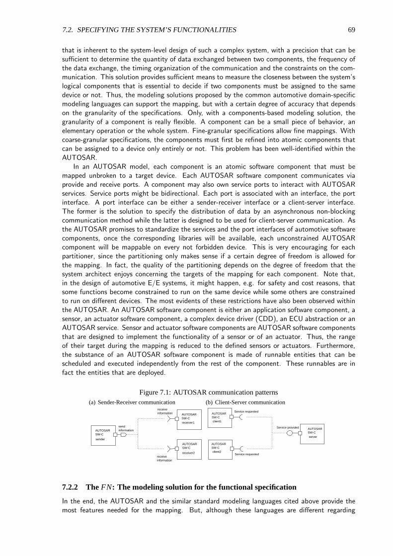
7.2. SPECIFYING THE SYSTEM’S FUNCTIONALITIES 69
that is inherent to the system-level design of such a complex system, with a precision that can besufficient to determine the quantity of data exchanged between two components, the frequency ofthe data exchange, the timing organization of the communication and the constraints on the com-munication. This solution provides sufficient means to measure the closeness between the system’slogical components that is essential to decide if two components must be assigned to the samedevice or not. Thus, the modeling solutions proposed by the common automotive domain-specificmodeling languages can support the mapping, but with a certain degree of accuracy that dependson the granularity of the specifications. Only, with a components-based modeling solution, thegranularity of a component is really flexible. A component can be a small piece of behavior, anelementary operation or the whole system. Fine-granular specifications allow fine mappings. Withcoarse-granular specifications, the components must first be refined into atomic components thatcan be assigned to a device only entirely or not. This problem has been well-identified within theAUTOSAR.
In an AUTOSAR model, each component is an atomic software component that must bemapped unbroken to a target device. Each AUTOSAR software component communicates viaprovide and receive ports. A component may also own service ports to interact with AUTOSARservices. Service ports might be bidirectional. Each port is associated with an interface, the portinterface. A port interface can be either a sender-receiver interface or a client-server interface.The former is the solution to specify the distribution of data by an asynchronous non-blockingcommunication method while the latter is designed to be used for client-server communication. Asthe AUTOSAR promises to standardize the services and the port interfaces of automotive softwarecomponents, once the corresponding libraries will be available, each unconstrained AUTOSARcomponent will be mappable on every not forbidden device. This is very encouraging for eachpartitioner, since the partitioning only makes sense if a certain degree of freedom is allowed forthe mapping. In fact, the quality of the partitioning depends on the degree of freedom that thesystem architect enjoys concerning the targets of the mapping for each component. Note that,in the design of automotive E/E systems, it might happen, e.g. for safety and cost reasons, thatsome functions become constrained to run on the same device while some others are constrainedto run on different devices. The most evidents of these restrictions have also been observed withinthe AUTOSAR. An AUTOSAR software component is either an application software component, asensor, an actuator software component, a complex device driver (CDD), an ECU abstraction or anAUTOSAR service. Sensor and actuator software components are AUTOSAR software componentsthat are designed to implement the functionality of a sensor or of an actuator. Thus, the rangeof their target during the mapping is reduced to the defined sensors or actuators. Furthermore,the substance of an AUTOSAR software component is made of runnable entities that can bescheduled and executed independently from the rest of the component. These runnables are infact the entities that are deployed.
Figure 7.1: AUTOSAR communication patterns(a) Sender-Receiver communication
AUTOSAR SW-C
sender
receive information
receive information
send information
AUTOSAR SW-C receiver1
AUTOSAR SW-C
receiver2
(b) Client-Server communication
AUTOSAR SW-C
AUTOSAR SW-C
AUTOSAR SW-C
client1
client2
server
Service requested
Service requested
Service provided
7.2.2 TheFN: The modeling solution for the functional specification
In the end, the AUTOSAR and the similar standard modeling languages cited above provide themost features needed for the mapping. But, although these languages are different regarding

70 CHAPTER 7. INPUTS FOR THE PARTITIONING
the semantics that they give to the model elements, they are collectively lacking the semanticalprecision that would support a computer-based mapping. For example, extracting the data thatis exchanged on the arms of a branched connector necessitates more screening and analysis effortthan on unbranched connectors. We thus added the following semantical precisions to the provedcomponents concepts (i.e. atomic components, ports, interfaces and connectors) and the QoSmodeling capabilities provided by the above languages to define a more intuitive modeling solutionthat meets the requirements of our CAD-supported partitioning: A component is either a functionalbehavior or a data component, i.e. a data repository, a variable or a memory. A data componentis given the semantics of a behavior providing read and write functionalities on the containeddata. Like in AUTOSAR, each component is an atomic component. It owns a set of portsthrough which it communicates with its environment. The set of ports of a component is thecomponents interface. Each port is associated with exactly one port interface. A port interface issolely a container for the information exchanged via the associated port. Such an interface mustnot implement an API for itself, but it rather describes the information exchanged through theassociated port (i.e. data or service). The communication between the components is materializedby means of connectors. A connector is simply a materialization of a connection between twocomponents. It aims at specifying a communication path. This modeling solution underlies thefollowing rules:
• The range of a data object is limited within the connector on which it is transported. If apiece of data is found on different connectors, that means that it is steadily ignored by all theintermediate components. This is important to achieve the tracing of the communicationdata since with this property the emitter and the receiver of each data object can be directlyidentified by a simple observation of the data object.
• Each connector has only one originating and one destination component. The profits of thisproperty are clearly illustrated in the example shown in figure 7.3 where the communicationpaths within the functional specification of the system under design are clearly identifiable.
• Ports are exclusively unidirectional (also see figure 7.3). Unlike the standard languages, wedo not allow bidirectional connectors or ports. The direction of the communication is assignificant for the issue of the partitioning as the amount of data exchanged. Often, thedata exchanged between two ports is different from one direction to the other. This cannotbe usefully modeled on a bunched connector as done in AUTOSAR model for example.Furthermore, with bidirectional ports, we deal with hyper graphs, making the partitioningproblem harder.
• Only ports of opposite directions can be connected, namely in the direction going from anoutput port to an input port.
• All the information contained in a port interface must have the same direction. Only input(i.e. required) information can be modeled on an input port and only output (i.e. provided)information can be modeled on an output port or a provider interface.
• A connector relates exactly two ports. Only the ports of different components can beconnected. Consequently, a connector can be identified by its originating and its destinationport. The number of connectors connecting two components is an important closeness metricsince it measures the width of the connection that is an important indicator of the relativeimportance of a connection.
• Between a pair of ports, there can exist one connector at maximum.
• The set of information flowing on a connector is the intersection of the interfaces of theoriginating port and the destination port. We define this as the interface of the connector.

7.2. SPECIFYING THE SYSTEM’S FUNCTIONALITIES 71
As this model is a network of logical components, we call it FN for ”Functional Network”.Formally, a FN model is a weighted graph, each node of which is either an atomic functionalcomponent or an atomic data component and the edges are the connectors described above. Wecan now define the FN as the following quintuple:
Definition 7.1 (FN:). EachFN model can be formally defined with a quintuple〈F,R,P, I ,C〉 in which:
• F (Functions) is the set of all the behavioral components in the model, i.e.F =
F1,F2, ...,Ff
where eachFi represents a functional component;i, f ∈ N
• R (Repositories) is the set of all data components in the model, i.e.R= R1,R2, ...,Rr whereeachRi represents a data component;i, r ∈ N
• P (Ports) is the set of input and output ports, i.e.P = P1,P2, ...,Pp i, p∈ N with P = IPorts⊕OPorts(i.e. Input ports⊕ Output ports)
• I (Interfaces) is the set of all the port interfaces in the model, i.e.I = I1, I2, ..., Ip where eachIi represents the interface of the porti; i, p∈ N
• C (Connectors) is the set of all connectors in the model, i.e.C = C1,C2, ...,Cl where eachCi
represents a connector;i, l ∈ N
• Each componentFi or Ri is defined by its internal behaviorbehand its interfaceInt, i.e. eachcomponent is completely defined by a tuple< beh, Int > with Int ⊆ P andbehis defined by therunnables
• Each portPi is defined by its behaviorbeh and its interfaceInt, i.e. Pi =< beh, Int > withPi .Int ∈ I
• For each connectorCi , ∃src∈ OPort, dst∈ IPort and Int so thatCi =< src,dst, Int > whereCi .src is the port source of the connectorCi , Ci .dst is the port destination of the connectorCi andCi .Int is the set of the data that might flow onCi ; Ci .Int = Ci .src.Int ∩Ci .dst.Int
Figure 7.2 illustrates the relationships between the FN and the standards.
is AES domain-specific
<<meta-model>> UML 2.0
<<meta-model>> SysML
<<meta-model>> AUTOSAR
Partitioning-Compliant language FN
<<profile>> SysML UML Profile
<<profile>> AUTOSAR UML Profile
<<importFrom>>
<<instanceOf>>
<<instanceOf>>
<<reuse>>
<<reuse>>
<<reuse>>
<<instanceOf>>
is general-purpose
<<meta-model>> EAST ADL
<<profile>> EAST ADL UML Profile
is AES domain-specific
is general-purpose
<<importFrom>><<importFrom>>
<<customize>>
<<customize>>
AES domain-specific
standard
<<importFrom>>
<<importFrom>>
<<importFrom>>
Figure 7.2: TheFN inherits the common concepts from the standards
Figure 7.3 shows a graphical representation of a part of the specification of the ACC (activecruise control) following the FN modeling style. The functional components are atomic entities.

72 CHAPTER 7. INPUTS FOR THE PARTITIONING
The dashed frames represent the data objects that are accessible on the associated output portor that are demanded by the associated input port. These are the ports’ interfaces. The dataobjects contained in each output port interface are all output data (from the point of view ofthe associated components) while the data objects contained in the input port interfaces are allinput data, i.e. incoming data from the point of view of the component that is associated withthe port. Such a model meets the humans’ natural feeling. With the FN modeling format, thecapturing of the functionality of the system under design is as intuitive as the understanding ofthe resulting specification. The interface of the connector relating two ports is the intersection ofthe interfaces of these ports. For example, the interface of the connector between the componentsMax speed setting and Speed control overall contains solely the data object speed selection, thatis the only data object that is communicated through this connector. The remaining data objectsare communicated through different connectors, thus with different components. The interfacesof connectors will be further discussed and illustrated in the following chapter (see section 8.3).
speed_actual speed_regulation_state
acceleration_min set_distance_min
potencial_stationary_objects regulation_obl_objects
objects_sto
display_collision_alert display_driver_reation
max_acceleration obstacle_nomination
nominal_distance
speed_actual speed_lateral_state acceleration_angle nominal _distance acceleration_min obstacle_detection
objects_sto
Curve treatmentacceleration_limit_ped acceleration_limit_eng
display_speed limit_accelerationSpeed control
overall
speed_actual speed_regulation_state
acceleration_min speed_odometer speed_selection
distance_selection
tempomat_setting
display_distance set_distance_min display_max_speed
speed_selection
Max speed setting
Security distance setting
Obstacle screening
object_nomination speed_angle_wheel
radar_signal speed_actual
object_found state_radar_sensor
hor_just_state ver_just_state
object_found
speed_angle_wheel radar_signal speed_actual
Lane determination
lane_attributes
potencial_stationary_objects regulation_obl_objects
objects_sto
Obstacle identification
Speed control retarder
Figure 7.3: A partial graphical representation of the ACC’s functionality following theFN format
7.3 Specifying the hardware platform
7.3.1 Relevant modeling concepts
Automotive hardware platforms are networks of communicating multiprocessor systems (i.e. ECUs,sensors and actuators). The choice of a communication protocol follows the topology of theplatform and the design constraints. The latter include for example the demand for cost-efficiency,the real-time communication requirements and the requirements for fault-tolerance, robustness,etc. The functional and data components assigned to a device can be implemented on a varietyof hardware architectures. Depending on the design options, the device hardware can be a mono-or a multi-elements platform of processing units, memories and on-board communication systems.For example, as micro-controllers generally incorporate a wide variety of hardware modules, e.g.ADCs, I/O devices, timers, UART, SPI and I2C interfaces, RAMs, CAN transceiver, etc., theysometimes represent a good choice to implement a mono-component platform.
The AUTOSAR has defined a generic ”AUTOSAR ECU architecture” [22] containing the ap-plication software, the basic software and the hardware platform (see figure 7.4). The functionality,that is deployed on an ECU is modeled in the application layer. For each ECU, the correspondingRTE is tailored from the VFB so that only the interfaces and the services that are needed on thisparticular ECU will be effectively implemented. The RTE is the communication system relating theapplication layer with the basic software. The basic software implements the infrastructure services(e.g. hardware drivers, OS, ECU abstractions, etc.) and the communication protocols that areneeded on the ECU. The basic software layer has a components-based architecture, but it can be

7.3. SPECIFYING THE HARDWARE PLATFORM 73
organized in four abstraction layers like in figure 7.5. An example of hardware architecture is givenin the ECU-hardware layer. The platform consists of a microcontroller, an ASIC implementing forexample a CAN controller, and an external non-volatile memory (flash RAM), interfacing througha SPI or an I2C bus.
Complex
Drivers
Microcontroller
AUTOSAR Runtime Environment (RTE)
Microcontroller Drivers Memory Drivers I/O Drivers
I/O Hardware
Abstraction
Memory Hardware
Abstraction
Memory ServicesSystem Services
Onboard Device
Abstraction
Communication
Drivers
Communication
Hardware Abstraction
Communication
Services
Application Layer
Figure 7.4: The AUTOSAR ECU architecture (source: Autosar web content V2.0.1)
The ECU-hardware or Microcontroller layer contains the real hardware platform of the ECU.Such a platform may contain all types of processors (e.g. microcontroller, ASIC, ASIP, FPGA,DSP, ADC, etc.), memories (e.g. ROM, RAM, Flash, etc.) and communication buses.
The Microcontroller Abstraction Layer (MCAL) is the software model of the hardware platform.It contains the drivers for the internal1 hardware devices and the memory-mapped external devices(e.g. external flash), and other functions with direct access to the hardware like the test functionsfor the RAM or the core processor. The MCAL makes the upper layers of the ECU-softwareindependent from the hardware. It provides standardized interfaces between the hardware and theother components of the basic software that need access to the hardware.
The ECU abstraction layer is designed to make the higher software layers independent from theECU hardware layout. The ECU abstraction layer aims at hiding the location2 of the ECU hardwaredevices and their inter-connections. It contains the handlers3 and the drivers for some externaldevices, such as external EEPROMs, external watchdogs, etc.
The Services layer builds the larges interface of the basic software to the RTE. It contains thehigh-level services of the basic software, including the OS services, the vehicle network communi-cation and management services, the memory services, the diagnosis services and the ECU statemanagement services.
The Complex Device Driver (CDD) is a container for the basic software components that arenot defined within the AUTOSAR. This includes for example the drivers for hardware devicesthat are not supported or not foreseen by AUTOSAR such as a driver for the controller of a newcommunication system, a complex sensor or actuator control module, firmwares and proprietarydrivers, etc.
1External device is used in this context to identify a hardware device that is located on the ECU but outside the micro-controller. In opposition, a device that is located on the microcontroller is called internal device
2Internal devices are located on the microcontroller chip (on-chip) while external devices are on the ECU board (on-board)
3A handler is a specific function that controls and synchronizes the access to one or more drivers, i.e. it might performbuffering, queuing, arbitration or multiplexing

74 CHAPTER 7. INPUTS FOR THE PARTITIONING
SPI, I2C
Service Layer
-Basic services
for the
application and
basic SW
modules e.g. OS,
AUTOSAR
services,
diagnosis
service, NW
management,
etc.
System services
-Provide basic
services for
application and
SW modules,
e.g. RTOS, error
manager, library
functions.
Memory services=
NVRAM manager
-Abstraction of
memory properties
and location
-Provide data
management
services e.g.
saving, loading,
verification, etc.
-Provide uniform
interface for non-
volatile data access
Communication
services
-Provide uniform
interface for
vehicle NW
comm, e.g. for
CAN, LIN and
FlexRay
-Hide protocol
and message
properties from
the application
ECU
Abstraction
Layer
-SW modules
for the
abstraction of
the location of
the ECU-HW
devices and the
HW layout
Location=on
chip or onboard
Onboard device
abstraction
-Abstraction of
the special ECU
onboard self-
contained
devices
-Contains
drivers for
specific, non
usual ECU
onboard devices
e.g. external
watchdog,
system basic
chip, etc.
Memory-HW
abstraction
-Hide the location
of the memories
-Offers memory-
specific interfaces
to access the
memory drivers
e.g. EEPROM
interface, RAM
interface
-Offers common
mechanisms to
access internal and
external memories
Communication-
HW abstraction
-Hide the location
of the ECU-
communication
controllers and
the ECU layout
-Offers bus-
specific interfaces
to access the
comm. drivers
e.g. LIN, CAN,
MOST interface,
SPI, I2C interface
-Provides uniform
bus access
mechanisms
I/O HW
abstraction
-Hide the
location of the
peripheral I/O
devices
-Hide the ECU-
HW layout
-Offers common
I/O signal
interface for
accessing the I/O
devices
MCAL
- Drivers for the
HW devices and
functions with
direct access to
HW devices e.g.
test functions for
RAM, core
processor, etc.
mC drivers
-For internal
(on-chip)
peripherals e.g.
ADC, clocks,etc.
-For functions
with direct mC
access e.g. RAM
test, core test
Memory drivers
-For internal (on-
chip) memories e.g.
int. Flash, int.
EEPROM
-For ext. (onboard)
memories e.g. ext.
flash, external
EEPROM
Communication
drivers
-Drivers for ECU
onboard comm
e.g. SPI, I2C
-Drivers for
vehicle comm e.g.
CAN, FlexRay,
LIN
I/O drivers
- For analog and
digital I/O e.g.
ADC, PWM,
DIO
ECU HW,
Microcontroller
Layer
-HW Platform
i.e. buses,
microcontrollers,
memories,
ASICs, etc.
ADC CPU RAM
NVRAM e.g.
Flash RAM,
EEPROMInt CAN
controller
Timer
CAN controller
ASIC
(external)
Flash RAM
Figure 7.5: Overview of the AUTOSAR layered ECU architecture
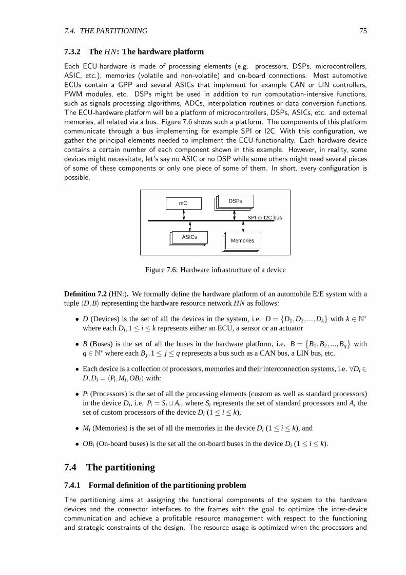
7.4. THE PARTITIONING 75
7.3.2 TheHN: The hardware platform
Each ECU-hardware is made of processing elements (e.g. processors, DSPs, microcontrollers,ASIC, etc.), memories (volatile and non-volatile) and on-board connections. Most automotiveECUs contain a GPP and several ASICs that implement for example CAN or LIN controllers,PWM modules, etc. DSPs might be used in addition to run computation-intensive functions,such as signals processing algorithms, ADCs, interpolation routines or data conversion functions.The ECU-hardware platform will be a platform of microcontrollers, DSPs, ASICs, etc. and externalmemories, all related via a bus. Figure 7.6 shows such a platform. The components of this platformcommunicate through a bus implementing for example SPI or I2C. With this configuration, wegather the principal elements needed to implement the ECU-functionality. Each hardware devicecontains a certain number of each component shown in this example. However, in reality, somedevices might necessitate, let’s say no ASIC or no DSP while some others might need several piecesof some of these components or only one piece of some of them. In short, every configuration ispossible.
mC DSPsDSP 2DSPs
ASICASICASICsMemoriesMemoriesMemories
SPI or I2C bus
Figure 7.6: Hardware infrastructure of a device
Definition 7.2 (HN:). We formally define the hardware platform of an automobile E/E system with atuple〈D,B〉 representing the hardware resource networkHN as follows:
• D (Devices) is the set of all the devices in the system, i.e.D = D1,D2, ...,Dk with k ∈ N∗
where eachDi ,1≤ i ≤ k represents either an ECU, a sensor or an actuator
• B (Buses) is the set of all the buses in the hardware platform, i.e.B =
B1,B2, ...,Bq
withq∈ N
∗ where eachB j ,1≤ j ≤ q represents a bus such as a CAN bus, a LIN bus, etc.
• Each device is a collection of processors, memories and their interconnection systems, i.e.∀Di ∈D,Di = 〈Pi ,Mi ,OBi〉 with:
• Pi (Processors) is the set of all the processing elements (custom as well asstandard processors)in the deviceDi , i.e. Pi = Si ∪Ai , whereSi represents the set of standard processors andAi theset of custom processors of the deviceDi (1≤ i ≤ k),
• Mi (Memories) is the set of all the memories in the deviceDi (1≤ i ≤ k), and
• OBi (On-board buses) is the set all the on-board buses in the deviceDi (1≤ i ≤ k).
7.4 The partitioning
7.4.1 Formal definition of the partitioning problem
The partitioning aims at assigning the functional components of the system to the hardwaredevices and the connector interfaces to the frames with the goal to optimize the inter-devicecommunication and achieve a profitable resource management with respect to the functioningand strategic constraints of the design. The resource usage is optimized when the processors and
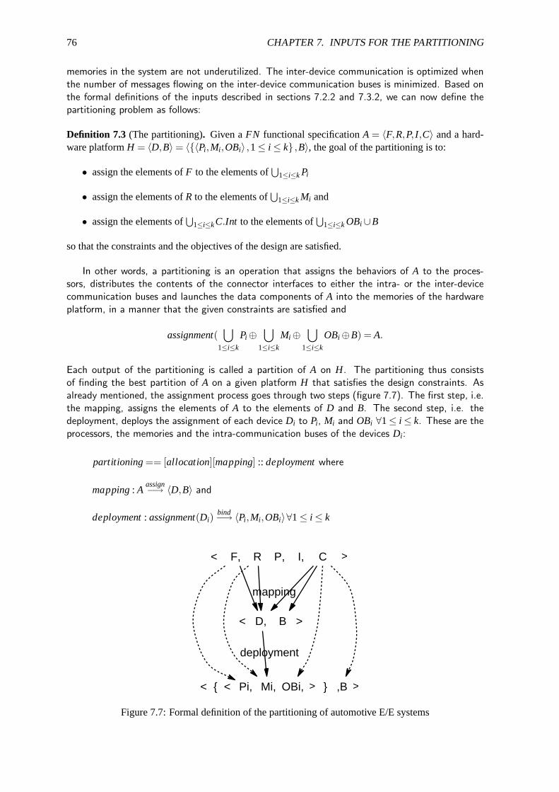
76 CHAPTER 7. INPUTS FOR THE PARTITIONING
memories in the system are not underutilized. The inter-device communication is optimized whenthe number of messages flowing on the inter-device communication buses is minimized. Based onthe formal definitions of the inputs described in sections 7.2.2 and 7.3.2, we can now define thepartitioning problem as follows:
Definition 7.3 (The partitioning). Given aFN functional specificationA = 〈F,R,P, I ,C〉 and a hard-ware platformH = 〈D,B〉 = 〈〈Pi ,Mi ,OBi〉 ,1≤ i ≤ k ,B〉, the goal of the partitioning is to:
• assign the elements ofF to the elements of⋃
1≤i≤k Pi
• assign the elements ofR to the elements of⋃
1≤i≤k Mi and
• assign the elements of⋃
1≤i≤kC.Int to the elements of⋃
1≤i≤k OBi ∪B
so that the constraints and the objectives of the design are satisfied.
In other words, a partitioning is an operation that assigns the behaviors of A to the proces-sors, distributes the contents of the connector interfaces to either the intra- or the inter-devicecommunication buses and launches the data components of A into the memories of the hardwareplatform, in a manner that the given constraints are satisfied and
assignment(⋃
1≤i≤k
Pi ⊕⋃
1≤i≤k
Mi ⊕⋃
1≤i≤k
OBi ⊕B) = A.
Each output of the partitioning is called a partition of A on H. The partitioning thus consistsof finding the best partition of A on a given platform H that satisfies the design constraints. Asalready mentioned, the assignment process goes through two steps (figure 7.7). The first step, i.e.the mapping, assigns the elements of A to the elements of D and B. The second step, i.e. thedeployment, deploys the assignment of each device Di to Pi , Mi and OBi ∀1≤ i ≤ k. These are theprocessors, the memories and the intra-communication buses of the devices Di :
partitioning== [allocation][mapping] :: deploymentwhere
mapping: Aassign−→ 〈D,B〉 and
deployment: assignment(Di)bind−→ 〈Pi ,Mi ,OBi〉∀1≤ i ≤ k
< F, P, I, C >R
< Pi, OBi, ,B >Mi,< >
B >< D,
mapping
deployment
Figure 7.7: Formal definition of the partitioning of automotive E/E systems

7.4. THE PARTITIONING 77
7.4.2 Relevant attributes for the elements of the input models
The partitioning is guided by the resource needs of the functional specification and the capacityof the platform. The input specifications must be enhanced with partitioning-relevant informationsuch as the resource requirements of the components of the functional model and their connections,and the amount of resource that is available on the platform. In our input models, this informationis specified in the form of attributes. The attributes of the elements of the functional specification(i.e. components, connectors, interfaces, ports) that are relevant for the partitioning are mainlythose concerning the consumption of memory, of execution time and of communication bandwidth.The resource consumption of a functional component includes the execution time and the amountof memory needed to store the compiled code (e.g. the object file), the data that is necessary forthe component’s behavior and the data that is exchanged with its environment. Connectors andinterfaces consume the communication bandwidth or (as variables) the memory. The resourcesthat are available on the infrastructure platform, i.e. hardware devices (ECU, actuator or sensor)and buses, are the amount of computation power, memory and communication bandwidth thatcan be used by the application software on this platform. The hardware resources can be dividedinto static and dynamic resources. Static resources, e.g. ROM, are assigned for occupationonce and kept unchanged. Dynamic resources, for example processors or RAMs can be occupieddynamically by the different consumers that need to share them. In the following, we introducesome partitioning-relevant attributes of the elements of the input models:
Functional components: The attributes describing a functional component that are relevant forthe partition include:
• The execution time: The duration (in seconds) of the execution of the code of the componenton a given CPU. This is the time required between the starting of the execution of thecomponent and its finishing. Alternatively, the execution time of a data component is theduration of a read or write operation on the memory on which the data is stored. Eachdata component may thus also have several execution time values depending on the type ofmemory on which it is stored.
• The execution rate: The period (in seconds) of execution of a behavior. Alternatively, theperiod of execution of read and write operations on a data component.
• The software code size: The amount (in bytes) of memory required to store the code of thefunctional component when implemented in software. Alternatively the amount of memoryneeded to store the data component.
• The hardware size: The amount of hardware material (in number of gates, transistors orlogic blocks) that would be used to implement the software component in hardware.
• The basic software: The list of compatible (versions) of basic software modules that areneeded by the components.
• The hardware element: The processor type with which the actual implementation is com-patible. Alternatively the type of memory that is appropriate to store the data component.
Interfaces: An interface is a container for the data flowing through the associated port. Like inAUTOSAR, the interfaces in FN models describe the static structure of the data. The interfacedata itself consists either of data elements or operations. Data elements are described by meansof data types. Operations are described through their signatures, i.e. the arguments that arecommunicated between the client and the server. Each argument of a signature has a direction (in,out or inout) and also a data type. For reasons of syntactical clarity, we subsume the informationthat is exchanged between the nodes of FN models under the common aspect of data objects.The logic of this abstraction is shown in figure 7.8.

78 CHAPTER 7. INPUTS FOR THE PARTITIONING
sender-receiver interface
client-server interface
data elements
operations arguments
data object
*
* *
1
1 1
Figure 7.8: Data object is a generalization of operations and data elements
Data objects: The relevant attributes of data objects include:
• The direction: In, out or in-out direction.
• The resolution: The number of bits that is necessary to store the data object. At theimplementation level, the resolution of a data object may variate depending on the mediumtransporting it (e.g. CAN or SPI) or the machine on which it is implemented (e.g. big-endian, little-endian), but at the logical level, the value of the attribute resolution is notsupposed to change. For example, if the size of the structure in which a data element isstored is 12 bits, the resolution of this data element will be considered as equal to 12 bitsand every possible conversion of the data element will be ignored.
• The access frequency: This attribute indicates the frequency at which the data object isaccessed, i.e. the number of times the data is read during a given period. For exampleduring an execution time of the source component.
Ports: The attributes describing a port include:
• The resynchronization time: The time allowed for the resynchronization of the data valuesafter the current data is lost, e.g. after an ECU reset.
• The timeout: The time (in seconds) between the activation of the port and its time out.
Connectors: Relevant attributes of the connectors include:
• The latency: The maximum time allowed for the transfer of a data element from the sourcecomponent to the destination.
• The jitter: The maximum allowed jitter as a measure of the variance of transport time.
Processors: Examples of the attributes of a processor include:
• The processing power: The speed of computation (in mips, i.e. machine instructions perseconds) of the CPU for standard processors.
• The architecture: The composition and the structure of the processor, the computing paths,the elementary operations, etc.
Memories: Memories can be classified in two categories: Volatile memories and Non-volatilememories. Volatile memories require power to maintain the stored information, e.g. RAMs. Non-volatile memories can retain the stored information even when the power supply is off. Examplesof non-volatile memories include ROMs, flash memories and NVRAMs (Non-Volatile RAMs, e.g.flash RAMs). Examples of attributes of volatile memories include:
• The segment size: The size (in Byte) of one memory segment.

7.5. CONCLUSION 79
• The access type: Read only or also written memory.
• The access time: The mean time for a read, write or erase operation.
• The location: Internal (on chip), external memory (on-board) or stand-alone memory (de-vice).
In addition to these attributes, non-volatile memories can be characterized by:
• The data retention time: The mean time during which a data is valid within a memorysegment.
• The endurance: The number of guaranteed data changes on the memory.
Buses: Examples of the attributes of hardware connections include:
• The bandwidth: The bit rate, i.e. the amount (e.g. in bps, i.e. bits or bytes per seconds) ofdata that can be transmitted throughout the bus in a fixed amount of time.
• The jitter: The time deviation from the ideal timing of data transmission. The jitter on abus can follow a random (statistical dispersion) or a deterministic behavior.
7.5 Conclusion
The standard languages provide powerful features to model AES, but because the semantics ofports, interfaces and connectors are fuzzy, they remain very insufficient to support the partition-ing. For the functional specification, we have defined a modeling solution that is based on themost common AES specification languages like AUTOSAR, EAST ADL and SysML, so that wekeep very close with standards. We enhanced the basic concepts provided by these languages inorder to obtain a modeling solution that is fitter regarding the requirements of a CAD-supportedpartitioning. In addition to the partitioning-friendly features provided by AUTOSAR, EAST ADLand SysML, i.e. atomic detachable components, QoS modeling, etc., the FN provides a clearscreening of the communication paths, very useful for the partitioning. We also formally definedthe modeling concepts for the specification of AES hardware platforms that allowed us to define thepartitioning problem more precisely and formally. However, even at this point in the progression ofour work, we have not definitely answered the question relative to the ability of the input modelsto support a CAD-based partitioning, i.e. Are these models sufficient for the partitioning? If not,how to make them more partitioning-friendly? These questions will be answered in the followingchapter.

80 CHAPTER 7. INPUTS FOR THE PARTITIONING

Chapter 8
The synthesis Model
In the actual state-of-the-art, AES designers input a functional specification in the form of a network ofsoftware components (like a FN model) and a HW platform specification in the form of interconnecteddevices (e.g. a HN model). This models might be explicit enough to describe the system, but they arenot optimized to support the partitioning of the system specification. We needsynthesizable modelsthat can enable the analysis of the data flow and highlight the closeness between the elements of thespecification. In this chapter, we define the synthesis model, i.e. the modeling format that will be usedto support the partitioning of AES functional specifications, and the transformation rules that shallgovern the translation of an input FN model into this modeling format.
8.1 Definition of the synthesis model
8.1.1 Requirements for the synthesis model
The FN allows clear screening of the communication paths and the tracing of the data flowing uponeach connector. But, in order to solve the partitioning problem, we need to transform each FNmodel into a formal representation on which we can use efficient and reliable mathematical toolsto perform data flow analysis and quantify the relationships between the elements of the functionalspecification of the system. This will be achieved through the definition of an intermediate modelthat we call the synthesis model. The usefulness of a synthesis model is given by its ability tosupport the intended design task, in the present case, the partitioning. This includes the ability toreflect the system architecture as given in the FN input model, the ability to specify the informationthat is needed for the partitioning and the ability to enable rapid estimation of the partitioningmetrics. Reflecting the system architecture requires that the intermediate model must be at leastat the same level of granularity with the input FN model. A FN model is made of atomic softwarecomponents like those described in AUTOSAR. The synthesis model must allow to estimate andcompare the closeness between different pairs of components. Enabling rapid metrics estimationsrequires that as much information as possible is known before the partitioning begins, e.g. theaccess frequencies, the timing behaviors of the inter-components communications, the quantityof data exchanged, the relationships between these data objects and between the componentsthemselves, etc.
Depending on the type of representation used, the formal representations that meet the re-quirements for the synthesis model can be roughly classified in two groups: Those based on FSMsand Petri nets and those based on graphs. In contrast to graph-based representations that considera unique system state, FSMs [123] and Petri nets [35,119] are powerful in modeling and verifyingthe dynamics of a system. But, FSMs- and Petri nets-based representations are obviously not thebest representation forms for systems for which the architecture is important. The main kinds ofarchitecture-oriented forms of FSMs used in the design of embedded systems include the FSM withdata paths (FSMD) [53] and the FSM with Coprocessors (FSMC) [75]. But even these specialforms cannot reproduce the system’s architecture in a useful way. Moreover, they considerably
81

82 CHAPTER 8. THE SYNTHESIS MODEL
suffer from the state explosion problem. In the end, as our input models are not aware of any stateinformation, FSMs and Petri-nets are certainly not the solution for our synthesis model.
In contrast, because they more easily reflect the architecture of the system, graph-based rep-resentations have been largely used to solve partitioning problems. The most usual graph-basedmodels include data flow graphs (DFG)[38,95], control flow graphs (CFG), data control flow graphs(DCFG)[69] and task graphs. A DFG is a directed acyclic graph in which the nodes represent thesystem components and the edges represent the data flow. DFGs are well-featured to describethe data dependencies. A CFG is a directed graph of behavioral components in which the edgesrepresent the sequencing of the operations, i.e. the execution order of the nodes. CFGs are well-suited to model control-oriented systems, but they provide restricted facilities for the data flowanalysis. CDFGs extend the DFG with control nodes. They provide good models for data floworiented applications for which the control information is important. Task graphs are similar withDFGs in their structure. But, in opposition to DFGs, special types of task graphs may be cyclic orundirected [26,95,122]. Following the configuration of the input models and the requirements forthe synthesis model, such a special form of a task graph is probably the solution to our problem.
Various special task graph-based modeling formats have been used for similar problems. In [89],a data flow machine that is built of networked rings is used to analyze the data flow in a network ofprocessors and memories. In [115], a directed task graph, called access graph, is used to model theaccesses (i.e. data exchange) between the functional components of the system, while a similar,but undirected graph, called communication graph is used in [21] to model the communicationbetween a set of tasks. All these solutions yield static models that however effectively reproducethe system’s structure and the data dependencies.
8.1.2 The synthesis model
The synthesis model is intended to specify the components of the system, their communicationand all relevant relationships between them. We chose to represent each synthesis model witha task graph (V,E,Ω,S). Each node vi ∈ V represents a behavioral or a data component ofthe corresponding (FN) input model. If each connector of FN is replaced by an edge in thesynthesis model, this will be a multigraph, i.e. a graph with multiple edges between two nodes.Synthesizing the communication between two nodes that are related by multiple edges is much morecomplicated than when each two collaborating nodes are connected by a single edge. However,reducing multiple connectors to a single one requires that we must ignore the directions of theoriginal connectors. This leads to undirected edges. Undirected edges keep the synthesis modelsafe from the specification of the direction of the communication and consequently enable theunification of the connectors regardless of their individual directions. Therefore, with undirectededges, each edge ei j = (vi ,v j) = (v j ,vi) ∈ E materializes the communication between the FNcomponents represented by vi and v j . Such an edge thus models exclusively the fact that twonodes exchange data in a direction that is ignored by the edge itself or in the two directions. Thus,in the context of the synthesis model, ”edges” and ”connectors” are semantically identical withthe adoption of undirected edges, i.e. the semantics of an edge in the synthesis model is reducedto: ”These connected nodes represent two FN components that exchange data in some way”.
Evidently, transforming multiple and oppositely directed connectors into a single undirectedlink gives rise to two problems: Firstly, we need a convenient interpretation of the connectionswith multiple connectors that will allow to properly capture the data shared between the connectednodes on a single edge. Secondly, as the edges are undirected, we have to specify the directionof the communication somewhere else. The direction and the timing of the communication areessential for the mapping in a frames-oriented communication network, since a device is concernedonly with the packaging of the data objects that it sends, but not with the objects that it receives.The packaging and the sending of the tokens are submitted to the constraints concerning thedates of their occurrences and the dates at which they are sent. In order to bundle severaldifferently directed connectors into a single edge, it is necessary to separate the data objects from

8.1. DEFINITION OF THE SYNTHESIS MODEL 83
the connectors. To do that, we model the data that is exchanged between the nodes of thesynthesis model by means of tokens. Ω is the set of the tokens flowing around the graph. Atoken Tk
i j ∈ Ω represents the data object k that is exchanged between two nodes vi and v j . Atoken is unbounded in the dimension and is not supposed to contain any additional informationsuch as token delimitation information (i.e. begin of token, end of token), etc. Independentlyof the connector through which a data object is exchanged in FN, the corresponding token Tk
i jis associated with the edge ei j that connects the nodes vi and v j . Thus, the set of the tokensassociated with an edge models the intensity of the communication between the two nodes. Now,as the edges are undirected, we model the direction of the communication in the tokens. Thedirection of a token defines the sense of the data transfer on the corresponding edge, i.e. a tokenhas a source and a destination node, both related by the associated edge. So, due to the directionof the tokens, we can distinguish the data sent by a node to another node within the total dataexchange between two nodes. Remember that we defined a connection in FN as the interfacingbetween two components, i.e. the bundle or the set of all connectors connecting two components(see chapter 6).
This definition of the synthesis model leads to the following straightforward transformation ofFN models into synthesis models:
• Each component of a FN model is transformed into a node in the corresponding synthesismodel.
• Each connection of a FN model is transformed into a single edge in the correspondingsynthesis model.
• Each data object exchanged between two components of a FN model is transformed into atoken in the corresponding synthesis model.
For illustration, suppose the case of a client-server communication in which a client componentvi produces a token Tk
i j and sends it to a component v j (destination of Tki j ). v j performs the
necessary job with the received data and responds to the client using two tokens, lets say Tmji and
Tnji . In the corresponding (FN) model, this transaction is modeled by two connectors: One going
from the client to the server with the token Tki j and the other one going in the opposite direction
with the tokens Tmji and Tn
ji . But in the synthesis model, the two operations, i.e. the sending andthe response, will be modeled by means of a single undirected edge ei, j associated with the threetokens Tk
i j , Tmji and Tn
ji . However, due to the direction of the tokens, we can distinguish that token
Tki j is transferred from vi to v j while Tm
ji and Tnji flow in the opposite direction. Like the nodes and
the edges, each token has a system-wide identifier. This allows us to smoothly identify the tokensamong the whole system specification. In fact, the identification of a token is directly related withthe corresponding data object and the associated edge, i.e. if the same data element is transferredrepeatedly over a given edge, then it will be identified as the same token.
Several mechanisms can be used on this basic model to describe the data-passing procedure.For example, a node can send data by placing it on the dedicated edge, i.e. the token is addressedexclusively to the node connected at the other end of this edge, or the sender can just put thetoken on its output where it will be collected by the destination node. These two mechanisms arefundamentally different concerning the resulting behavior of the system. The first one processes apeer-to-peer communication while the second one, if not enhanced with restrictive routing rules,is merely adapted to realize broadcast communication, i.e. each component that is related withthe sender can access the data that is on the sender’s output port. Note that it is also conceivablethat the sender node pushes the data to the destination and so synchronous and asynchronouscommunication schemata can be designed. Defining such mechanisms would introduce a dynamicaldimension in the specification of the communication in the synthesis model. But, as the modelis not intended to support the simulation, the dynamics of the data exchange and the routingmechanisms will not be discussed in this paper. However, we agree that a token is created as soon
84 CHAPTER 8. THE SYNTHESIS MODEL
as the corresponding data object is emitted. We then say that the token is available. A token canbe sent to the destination nodes only if it is available. The date at which a token is sent is notnecessarily the date at which it is made available. A token is available solely means that the tokencan be sent. A token is available at the date of its creation. But it can be sent later, depending onits freshness requirements. So, while very hasty tokens must be sent as soon as they are available,the sending of less hasty tokens can be delayed. These concepts are introduced to support thescheduling of the communication and the control of the occupation of the communication bus.
In addition to the technical factors of performance and cost optimization such as the commu-nication and the resource usage optimization, the design of an E/E system typically underlies afull range of constraints and strategic concerns relative to the commercial, the technological andthe organizational conditions of the design, as well as the procurement and the production issues,etc. Consequently, some components of the functional model might be specified to run on thesame device while others are required to run on different devices. The latter is the case when forexample it is known that the implementations of two components are not EMC-compatible. Thecase of the components that must run on different devices include the components that are knownto have a high potential to share special hardware resources, those that must preferably be builttogether by a given sub-contractor that has proved his competency in their specific production orthose between which the communication is so constrained that it is not acceptable to take therisk of separating them. It is also conceivable that it may be profitable to group or to separate thecomponents following for example the similarities on their required level of safety, their level of mis-sion or business-criticality, the productivity capability of the source of procurement, the conditionsof production, etc. For illustration, components to be implemented in-house might be separatedfrom those to be implemented by sub-contractors and those to be implemented by COTS whilecomponents to be implemented by programmer X can be separated from those to be implementedunder the responsibility of Y. Further strategic relationships between the components might in-clude the potential level of reuse (i.e. typically reusable components vs. components with lowprobability to be reused), the rhythm of changing (i.e. frequently changing components vs. rarelychanging components), the target of the procured service, the activation time (e.g. componentsthat are active during driving vs. components that are activated during parking), componentsimplementing system internal services vs. components implementing system external services, etc.
These relationships between the components typically have heavy consequences on the par-titioning and must be specified in the synthesis model. We do this by means of needs andexcludes relations. Two nodes vi and v j are in a needs relationship, i.e. needs(vi ,v j), if they mustbe implemented on the same device. Two nodes vi and v j are in an excludes relationship, i.e.excludes(vi ,v j), if it is forbidden to implement them on the same device. Note that the needsand excludes relationships are also defined between the tokens. In relation with our taxonomy,all needs-related tokens build a message. Note also that indefinitely similar relationships can bedefined on this model. S is the set of these kinds of relations that exist between the nodes andbetween the tokens of a synthesis model.
In the remainder of this work, we will call this modeling format the ”Components Data FlowMachine (CDFM)”. The CDFM enables the synthesis of the communication by allowing thescanning of the data exchange and the tracing of the communication paths. However, it doesnot yet contain the information that is needed to guide the partitioning. In addition to themodeling of the components and the inter-components communication, a system partitioner needsthe information that will help to decide the destination device of each component and also enableto investigate the cost and the performance of the resulting partition. The CDFM provides theseinformation by means of the attributes that capture the runtime characteristics of the modelelements.

8.2. ANNOTATIONS FOR THE SYNTHESIS MODEL 85
8.2 Annotations for the synthesis model
8.2.1 Concurrency, sequencing
The information concerning the concurrency between the tasks of a system and their sequencingis certainly important for the partitioning. But, this is not actually explicitly specified in the FNmodels and thus must not be supported by the synthesis model. Nevertheless, as the connectorsspecify the data flow, they induce a certain level of data dependency information in the FN modelsthat is replicated in CDFM models, saving their affinity with the FN models. Anyway, we donot have concurrency and sequencing information at this level of the design where we are dealingwith software components the implementation of which might give rise to multiple tasks thatcan be scheduled in various processes depending on whether they need to run concurrently orsequentially. Thus, unless the components of a FN model consist each of a single task, we canneither establish concurrency or sequencing relationships between them, nor can they be reasonablyscheduled. However, as we firstly intend to map the components of the input FN models on thedevices of the E/E system, we do not need concurrency and sequencing information between them.Concurrency and sequencing information is more useful for the deployment and the scheduling ofthe ”runnables” within a device.
8.2.2 Annotations for the nodes
The performance and the cost of a node are determined by the duration of its execution, thefrequentness of its execution, the size of the resulting software code or the size of the hardwarethat should be needed to implement the component. While the size of the software code is easyto determine, the execution time of a component depends on the behavior of its runnables. Aslong as a component is not implemented, estimating its execution time is very difficult and even ifpossible, it might be useless to do that since the component will probably not be executed as a non-interrupted sequence of instructions. Actually, the most components are designed to encapsulate afunctionality that is well-known, thus the software code is known or can be estimated, but as theymostly result in several tasks at the runtime, it remains difficult to estimate their execution time.Estimated values are given as requirements for the implementation. Assuming that a particularhardware unit or a family of hardware units have been identified to implement or to store eachcomponent so that the memory needs for the code size and for the stacks or heaps for its runnablesare known (or can be estimated), the attributes of the nodes of the synthesis model include:
• The software size (swSize): The software size of a node is the total amount of memoryrequired to store the code and the data of the corresponding component when implementedin software. The software code size of a component depends on its implementation. Anefficient implementation of a software component may results in the consumption of lessmemory space. As we consider an optimistic resource reservation strategy, we can take forgranted that there is sufficient storing capacity on the platform to store the code of thenodes.
• The hardware size (hwSize): The hardware size of a node is the total amount of hard-ware components that would be used to implement the functionality of the correspondingcomponent.
• The execution rate (eR): The execution rate of a node is the maximum of the executionrates of the runnables of the corresponding component. The execution rate of a runnableis the number of times that it is executed during an activation time of the system. This isalso known as the frequency. If a runnable is periodically executed, its execution rate is easyto determine. For non-periodic runnables, we define the execution rate on the basis of themean interval between two successive executions. This assumption holds in the most casessince a large majority of tasks in embedded systems are periodic.

86 CHAPTER 8. THE SYNTHESIS MODEL
• The priority (prio): The priority of a node is the priority order of the most prioritizedrunnable of the corresponding component. The priority order of a runnable is the prioritythat it enjoys in the competition for the occupation of a given processor as assigned duringthe system design.
• The execution time (eT): If available, the execution time of a node is the ”sum” of theexecution times of the runnables of the corresponding component. The execution time ofa runnable is the time between the end of its triggering and the end of its execution. Theexecution time of a runnable depends on the processor on which it is executed and thecontext in which it runs. A runnable may thus be characterized by several execution timevalues, i.e. one execution time for each CPU on which it might run.
8.2.3 Annotations for the edges
The set of tokens associated with an edge is its weight. The determination of the weight of atoken is explained in section 8.3.1. An edge may underly some constraints such as the allowedmaximum transmission errors (i.e. the jitter) or the allowed maximum latency (i.e. transmissiontime). For illustration, the attributes of the edges of a CDFG model include:
• The weight (T): The weight of an edge is the set of tokens that flow over the edge duringan activation period of the system.
• The access frequency (accFreq): The access frequency of an edge is the access frequencyof the most accessed connector within the corresponding connection. The access frequencyof a connector is the number of times that the connector is accessed during an activationperiod of the system.
• The constraints (cons): The constraints on an edge are given by all the constraints on allthe connectors of the corresponding FN connection. The constraints on the edges mightinclude the latency, the reliability, the security, the safety, etc. Care must be taken to haveconsistent sets of constraints.
8.2.4 Annotations for the tokens
Concerning the tokens, the most relevant information for the partitioning include their dimension,their dates of occurrence, their freshness requirements, their direction and their priority, i.e. :
• The direction (dir): The direction of a token defines the sense in which it is transferred.Like the direction of the corresponding data object, the direction of a token is given by thesource node and the destination node of this token.
• The resolution (res): The resolution (or the dimension) of a token is the number of bitsthat is needed to encode the corresponding data object.
• The frequency (freq): The frequency of a token is the frequency at which the correspondingdata object is emitted.
• The priority (prio): The priority of a token is the priority level that the corresponding dataobject enjoys in the occupation of a given communication channel.
• The date of occurrence (occur): The date of occurrence of a token is the time at whichit is available. The tokens will be available in the same order with their dates of occurrence.The date of occurrence of a token is different from the date at which it is effectively sent(i.e. the sending date). The sending date of a token depends on the scheduling of thecommunication.
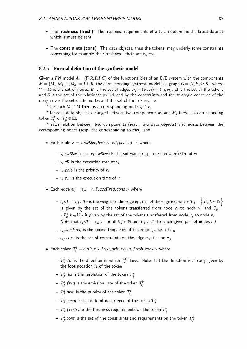
8.2. ANNOTATIONS FOR THE SYNTHESIS MODEL 87
• The freshness (fresh): The freshness requirements of a token determine the latest date atwhich it must be sent.
• The constraints (cons): The data objects, thus the tokens, may underly some constraintsconcerning for example their freshness, their safety, etc.
8.2.5 Formal definition of the synthesis model
Given a FN model A = 〈F,R,P, I ,C〉 of the functionalities of an E/E system with the componentsM = M1,M2, ...,Mk= F ∪R, the corresponding synthesis model is a graph G= (V,E,Ω,S), whereV = M is the set of nodes, E is the set of edges ei j = (vi ,v j) = (v j ,vi), Ω is the set of the tokensand S is the set of the relationships induced by the constraints and the strategic concerns of thedesign over the set of the nodes and the set of the tokens, i.e.
* for each Mi ∈ M there is a corresponding node vi ∈V,
* for each data object exchanged between two components Mi and M j there is a correspondingtoken Tk
i j or Tkji ∈ Ω,
* each relation between two components (resp. two data objects) also exists between thecorresponding nodes (resp. the corresponding tokens), and:
• Each node vi =< swSize,hwSize,eR, prio,eT > where
– vi .swSize(resp. vi .hwSize) is the software (resp. the hardware) size of vi
– vi .eR is the execution rate of vi
– vi .prio is the priority of vi
– vi .eT is the execution time of vi
• Each edge ei j = eji =< T,accFreq,cons> where
– ei j .T = Ti j ∪Tji is the weight of the edge ei j , i.e. of the edge eji , where Ti j =
Tki j ,k∈ N
is given by the set of the tokens transferred from node vi to node v j and Tji =
Tkji ,k∈ N
is given by the set of the tokens transferred from node v j to node vi .
Note that ei j .T = eji .T for all i, j ∈ N but Ti j 6= Tji for each given pair of nodes i, j
– ei j .accFreqis the access frequency of the edge ei j , i.e. of eji
– ei j .consis the set of constraints on the edge ei j , i.e. on eji
• Each token Tki j =< dir, res, f req, prio,occur, f resh,cons> where
– Tki j .dir is the direction in which Tk
i j flows. Note that the direction is already given bythe foot notation i j of the token
– Tki j .res is the resolution of the token Tk
i j
– Tki j . f req is the emission rate of the token Tk
i j
– Tki j .prio is the priority of the token Tk
i j
– Tki j .occur is the date of occurrence of the token Tk
i j
– Tki j . f reshare the freshness requirements on the token Tk
i j
– Tki j .consis the set of the constraints and requirements on the token Tk
i j

88 CHAPTER 8. THE SYNTHESIS MODEL
8.3 Applications
8.3.1 The weight of an edge in aCDFM model
We illustrate the calculation of the weight of an edge in a CDFM model with the following simpleexample. Suppose that two FN components are connected with a sender-receiver port interface,i.e. an interface through which they can exchange data elements, and a client-server interface, i.e.an interface through which operation calls can be initiated. Every 10 seconds, the first componentA1 sends for example the actual distance covered since the very first start of the system as read fromthe odometer to the second component A2. This is done through the sender-receiver interface.Then with a time interval of 1 minute, A1 triggers A2 periodically so that it calculates the totalmileage, i.e. the total number of kilometers that have been covered by the vehicle during thebeginning of the actual trip. The mileage is communicated to A1 that displays it to inform thedriver. This is done through the client-server interface. These two communication interfaces aremodeled in FN with three connectors (see figure 8.1). In fact, following the semantics of the FN,as A1 must receive the result of the mileage computation done by A2, the client-server interfacewill be modeled by two connectors, one from A1 to A2 and the other one from A2 to A1.
A1 A2
odometer_St
req_mileage
resp_mileage
Figure 8.1: The FN graphical representation of the mileage inquiry
The weight of the edge e12 of the corresponding CDFM model is the set of tokens exchangedbetween v1 and v2.
A1 A2
odometer_State req_mileage resp_mileage
Figure 8.2: The graphical CDFM representation of the mileage inquiry
We now define the metric that we use to determine the weight of the edges of CDFM models:Given a FN model A and its corresponding CDFM model G, consider the operator widthi j thatdefines the set of connectors of A that are represented by the edge ei j in G. These are theconnectors that relate Ai with A j . Assume that the operator srcConnectors(Ai) returns the setof connectors for which Ai is the source and the operator dstConnectors(Ai) returns the set ofconnectors for which Ai is the destination, i.e.:
srcConnectors(Ai) = c∈C|c.src∈ Ai .IntdstConnectors(Ai) = c∈C|c.dst∈ Ai .Intwidthi j = srcConnectors(Ai)∩dstConnectors(A j)
Given two nodes vi and v j of G, the weight of ei j (i.e. the set of tokens transferred over theedge ei j ) is:
ei j .T = Ti j ∪Tji =⋃
c∈widthi, j
c.Int (8.1)
Now, assuming that the resolution of the mileage is 16 bits, the parameters sent for theoperation call are altogether 72 bits (i.e. operation description, input values and addresses) andthe return value is 32 bits, we have:

8.4. CONCLUSION 89
|widthi, j | = 3 connectorsT12 = the 16 bits token, the 72 bits tokenT21 = the 32 bits token ande12.T = the 16 bits token, the 72 bit token, the 32 bits token
Given a period of time in which the system is activated, the frequencies of the tokens determinethe number of appearances of each token on the associated edge. For example if we consider thatthe sender-receiver connector is accessed 5 times during an activation period of A1 and the client-server connector is accessed 2 times during the same period, then:
T12 = 5 times the16 bits token + 2 times the72 bits tokenandT21 = 2 times the32 bits tokenThe date of occurrence of the tokens determines the order in which the tokens appear on an
edge, i.e. each token is emitted at a given date that determines its position in the sequence ofthe tokens associated with a given edge. Thus, the tokens associated with an edge can be orderedin a n-vector in ascending order following their date of occurrence where n is the total number oftokens transferred between two nodes during an execution period of the system.
8.3.2 Model transformation
The following example illustrates the transformation of FN models into CDFM models. Figure8.3 shows the CDFM model corresponding to the FN model of the ACC (active cruise control)functionality presented in figure 7.3.
Curve treatment
Speed control retarder
Lane determination
Obstacle screening
Speed control overall
Obstacle identification
Security distance setting
Max speed setting
objects_sto
object_found
state_radar_sensor
hor_just_state ver_just_state
lane_attributes
speed_selection
set_distance_min
potencial_stationary_objects regulation_obl_objects
objects_stonominal_distance
Figure 8.3: Model transformation: TheCDFM representation of theFN model of figure 7.3
8.4 Conclusion
The CDFM provides a powerful modeling format for the design of automobile E/E systems archi-tectures. These intermediate models are defined to allow the analysis of E/E system specifications,particularly the synthesis of the data flow for the partitioning. CDFM models are flexible as theycan be enhanced without limitation and they do not state any restriction on the granularity oftheir elements (i.e. nodes and tokens). CDFM models are obtained from a simple and straightfor-ward transformation of FN models. They provide a graph formulation of the system’s functionalspecification that enables the application of usual graph partitioning algorithms for the mappingas well as for the deployment.

90 CHAPTER 8. THE SYNTHESIS MODEL

Chapter 9
The partitioning: State-of-the-art
In this chapter we at first give a more concrete formulation of the partitioningproblem from which wededuce the requirements for the partitioning algorithms that are adequate forour problem. Then thestate-of-the-art in the partitioning is outlined. This includes a presentation of thedifferent partitioningmethods and the most popular classes of partitioning algorithms. We finally specify the algorithmicprocess of the partitioning.
9.1 The partitioning problem
9.1.1 Frames of the problem
We consider that the input functional model specifies the functionalities of a given AES functionaldomain, e.g. power train, comfort, multimedia and telematics, etc. that will be implemented ona network that does not integrate a gateway, e.g. a CAN, a MOST or a FlexRay bus. As themost AES inter-device communication protocols are message-oriented, we consider that the targetplatform architecture is made of the most popular of them, a CAN bus, on which the devices (ECUs,sensors, actuators) are connected. The partitioning will be done by grouping together-belonging,i.e. related components of the input functional specification, following a set of closeness patternsin order to build the functional clusters that will be mapped on the devices. A feasible partitioningwill result in clusters that respect the capacity of the devices and use no more than the availablestock of messages to communicate. This means that although extreme load-imbalance must beavoided, the partitioning is not reduced to a load-balancing problem, but is rather an optimizationproblem, i.e. the communication overhead must be minimized, the real-time communication ofthe system must be optimized, the resource utilization and the dependability of the system mustbe maximized by avoiding computing and communication faults. However, following the actualtrends in the automobile market, although the goal of this work is to avoid underutilization ofthe resources in order to prevent the overhead of costs due to unnecessary computing power andcommunication bandwidth, it is well-advised to have some reserve resources in the system wherenew functionalities can be implemented.
To solve this problem, the design space has to be explored with a strategy which at least con-verges toward a solution close to one which yields the optimal solution. Actually, AES architecturesare designed based on the designer’s inspiration. AES system designers are highly-experienced en-gineers that mostly act as system integrators, i.e. they order devices from components suppliersand plug them on the rest of the system. As they actually do this successfully, one can arguethat automatic partitioning tools might not perform competitively with humans. This assertion isperhaps reasonable when the input set of components and the partitioning patterns are reducedand easy to trace and to manage. But like most real-life problems, the design of AES architecturesinvolves the manipulation of very large sets of items with a large range of partitioning criteria thatare not always easy for a human intelligence to manage optimally. The level of expertise needed byhumans is very expensive as long as system architects are rather artists than engineers. A system
91

92 CHAPTER 9. THE PARTITIONING: STATE-OF-THE-ART
architect needs to invest a very long time to acquire this level of expertise and then it is veryadventurous to replace him. Furthermore, the solution space is often so large that humans willnever get time to scan it in order to pick out the best solution. With an automatic partitioning,we provide a powerful engineering tool for the design of AES architectures, helping this activity tomake the transition from its actual status of art to an engineering discipline.
In this work, we are concerned with the mapping. A mapping and definitely a partitioningcan be static or dynamic. In static mapping, the elements of the functional specification are as-signed to the platform elements prior to the execution and are not changed until the executionfinishes. Dynamic mapping is needed when the functional specification changes dynamically dur-ing the running time and needs to be redistributed. Based on the input functional specificationand the resource platform, static mappings can be classified following two taxonomies: The firstclassification is based on the specialization of the functional specification and/or of the platform.Following this classification, we can distinguish the mapping of specialized components on special-ized platforms, specialized components on arbitrary platforms, arbitrary components on specializedplatforms and arbitrary components on arbitrary platforms. The second classification is based onthe uniformity of the attributes of the elements of the functional specification (e.g. the attributesof the components and the weights of the connections) and the characteristics of the elements ofthe hardware platform. Following this classification, we can distinguish the mapping of uniformfunctional specifications on uniform platforms, non-uniform functional specifications on uniformplatforms, uniform functional specifications on non-uniform platforms and non-uniform functionalmodels on non-uniform platforms.
In our case, the partitioning problem is how to map CDFM models onto multi-device architec-tures of heterogeneous multi-processor hardware platform devices. Considering the CDFM, thisproblem is a graph partitioning problem. However, even though this work is focused on a spe-cialized domain, i.e. the automotive domain, the problem we address here is a static mapping ofa non-uniform graph of arbitrary components on an arbitrary non-uniform multi-device platformarchitecture, since the mapping is done once during the system conception and remains unchangedfor the whole life of the resulting system. Furthermore, a particular architecture might be used foryears on a wide range of product series. The functional components contained in the nodes of theCFDM models do not underlie neither a specialization nor a granularity constraint. They are justrequired to be atomic components. The communication data described in the tokens of the CDFMmodels might be of every possible nature, i.e. information, computation value, control directive,power supply, etc. The target platform is also unconstrained on the type and the capacity of itselements.
9.1.2 Requirements for the partitioning algorithm
Because of the wide range of its application fields, the partitioning of graphs have been widelyinvestigated. The most active research communities applying graph partitioning for the last decadeinclude the microelectronic design (e.g. for SW/HW co-design), the system analysis domain (e.g.for pattern- and similarity-based classification), the network engineering and the business manage-ment (to solve optimization problems). These communities have different terminologies, differentpatterns for the partitioning and make different compromises for the partitioning process. Butcommonly, the aim of the partitioning is to achieve a clustering of a given set of objects followingsome similarity patterns. As the overall goal of a partitioning algorithm is to find a global optimalsolution while performing as little computation as possible, it is necessary to identify the mostsuitable clustering techniques when solving a partitioning problem. A vast collection of clusteringalgorithms is available in the literature. Near general-purpose partitioning algorithms, a full rangeof specific-purpose algorithms have been designed. General-purpose algorithms propose genericsolutions while specific-purpose algorithms propose more effective solutions, each however opti-mized for a specific problem. Unfortunately, we are not aware of an algorithm for the partitioningof automotive systems functional specifications. Moreover, because clustering algorithms often

9.2. PARTITIONING METHODS 93
contain implicit assumptions about the cluster shapes, the measurement of the similarities and thegrouping criteria, there is no clustering algorithm that is universally applicable on all input struc-tures or with all possible clustering patterns. Thus, there is no competent perspective enablingsomeone to select one of the existing algorithms that is suitable for the problem at hand.
The usefulness of a partitioning algorithm is determined by its ability to match with the partic-ular problem under resolution and its complexity (in time and eventually in space). Matching theproblem includes the support of the format of the input specification with the involved artifacts (i.e.abstraction level, granularity), the capacity to accommodate the considered clustering patterns andthe organization of the clustering objects as well as the ability to produce good partitions. Thelatter involves the manner in which the clusters are formed and the sensitivity of the clusteringtechnique to changes that do not affect the intrinsic structure of the input objects, e.g. changesin the order of the input objects, or on the formulation of the clustering criteria. For our purpose,a partitioning algorithm must preserve the functional structure of the system (i.e. conservation ofthe connectivity within the input specification), allow user interaction (i.e. the system architectmust be able to impose the composition of the clusters at every time in the partitioning process)and afford the flexibility (i.e. the ability to rapidly integrate the changes occurring on the functionalmodel, the platform or the design constraints). To achieve good results, such an algorithm shallcertainly enjoy a global view on the system specification that enables the comparison of the close-ness between surrounding objects. As our partitioning is done for a static mapping of functionalspecifications on quite similar platforms of a wide range of vehicle series, the time and the spacecomplexity of the algorithm is not very critical. However, the algorithm must be able to find thebest result in the best possible time.
9.2 Partitioning methods
9.2.1 Exact and heuristic methods
A partitioning algorithm might make use of either exact or heuristic methods (figure 9.1). There aretwo broad approaches for exact methods. The first approach follows a systematic enumeration of allsolutions. This approach is not practicable when the solution space is very large like in the presentcase. The second approach makes use of linear programming methods. Linear programing is animportant modeling tool in operations research. It has been widely used in business managementto minimize the cost of production systems, in transportation to optimize the traffic flow, intelecommunication for routing problems, in microelectronics to optimize the cost of embeddedHW/SW systems, in the embedded software engineering for scheduling and allocation problemsand in a lot of other engineering and management fields. If there exist some points in the solutionspace where the objective function has the largest value, linear programming methods guaranteethat at least one of them will be found. The description of a problem through linear programsconsists of a linear function CTx, e.g. the objective function, that is to be maximized, the problemconstraints in the form Ax≤ B and a set of non-negative variables x ≥ 0, where x is a vectorof variables (representing for example the components of the cost function), C (representing forexample the weights of the components of the cost function) and B (the constraints) are vectorsof coefficients and A is a matrix of coefficients, e.g. a distance matrix. A linear program isusually expressed in matrix form and then becomes: Maximize CTx subject to Ax≤ B and x≥ 0.The most usual form of the linear programming method known in the partitioning of embeddedsystems is based on Integer Linear Programs (ILP), e.g. [105]. ILPs can be exactly solved bybranch-and-bound algorithms. But the problems with ILPs include the difficulty to solve theequations, the cost in time (exponential time-complexity) of ILP solutions and the difficulty tomodel non-linear constraints. Because of the complexity of the problem we are solving, even if wecould find an exact solution, linear programming would not be practicable due to the expensivecomputation time it would need (i.e. exponential runtime), the difficulty to model the constraintsas mathematical propositions and the loss of fidelity with the problem definition that will be

94 CHAPTER 9. THE PARTITIONING: STATE-OF-THE-ART
induced by the unavoidable assumptions. As the partitioning problems are generally NP-Complete[34, 54, 106], heuristic algorithms are the best way to find good solutions in a reasonable amountof time.
Heuristics attempt at finding optimal or nearly optimal solutions whereas no guarantee is givenon the optimality of the solution found. However, approximative methods, i.e. that find solu-tions whose proximity to the optimum is provable, can be applied to complete heuristic methods.Furthermore, problem-specific heuristics can use information about the problem both to acceler-ate the partitioning and to approach the optimal solution. Following the approach used, we candistinguish two groups of heuristics: Those using constructive techniques and those using parti-tional techniques (e.g. iterative improvement techniques). Constructive partitioning techniques arebased on clustering techniques. Given a set of objects and a partitioning problem on these objects,constructive partitioning techniques process by stepwise grouping these objects in order to achievea complete partition while partitional techniques determine all the clusters at once. Partitionaltechniques usually process by relocating (iteratively) the objects across the clusters to optimize anobjective function defined either locally (on a subset of the objects) or globally (over all of theobjects). Partitional methods have advantages in applications involving large sets of objects forwhich the construction of a dendrogram, i.e. a tree showing a sequence of clusterings where eachclustering is a partition of the set of objects, is computationally prohibitive. But in practice, parti-tional algorithms are generally used to refine an existing partition. As they do this iteratively, theyare also called iterative improvement algorithms. Nevertheless, some hybrid algorithms exploitingthe positive features of both the constructive and the partitional methods have been presented[102] but the results are obviously very poor, particularly concerning the time complexity of thealgorithms [73]. Most partitioning problems are solved using a combination of constructive anditerative algorithms whereas constructive algorithms are used to generate the start partition thatwill be refined iteratively. We also proceed in this way, i.e. we first construct a partition and thenwe use an iterative improvement algorithm to ameliorate the quality of this partition.
Partitioning Methods
Exact
Heuristic
Enumerative
LP
ILP
Random
Strategic
Constructive
Partitional
Hybrid
Agglomerative
Divisive
Enumerative
Move-Based (K&L, Tabu search)
EA (GA, ESs, EP)
SA
Deterministic
Stochastic
MILPDynamic ProgramingConstraint Programing
Random
Strategic
Figure 9.1: Taxonomy of the partitioning methods

9.2. PARTITIONING METHODS 95
9.2.2 Constructive partitioning techniques
The construction of a partition can be done by assigning randomly each object to a part of thepartition (random assignment) or by clustering the input objects using closeness (or distance)measures. Because random assignment methods are easy to implement and economical in com-putation time, they are used essentially to build the start partitions for improvement algorithms,i.e. partitions that will be refined. But, as the performance of the refinement procedures dependon the quality of the start partition, inputting randomly constructed partitions can significantlydamage the quality of the end-partition as well as the performance of the partitioning procedureitself. In fact, random assignment methods are characterized by the unpredictable quality of theirsolutions. Furthermore, they can completely destroy the connectivity of the system specification.Because of these shortcomings and the fact that they do not guarantee any quality for the result,random assignment methods will not be considered in this work.
Given a system of closeness patterns on a set of objects, clustering algorithms can classifythese objects following the values of their closeness measures to each other. Depending on theconfiguration of the problem to be solved through a clustering algorithm, we can process hierarchi-cally either with an agglomerative (bottom-up) or with a divisive (top-down) clustering. Divisivepartitioning algorithms follow a top-down splitting method. They start with all the objects in asingle cluster and successively split this cluster into smaller ones as desired or until each object fallsin one cluster. Divisive methods have been rarely applied to solve real-life partitioning problems.A divisive clustering algorithm is developed in [127]. It exploits the minimal spanning tree (MST)of the input set, i.e. the MST is constructed and the clusters are generated by deleting the edgeswith the largest lengths. Even though the time and space complexities of divisive algorithms aretypically lower than those of agglomerative algorithms, a typical divisive algorithm works well onlyon object sets containing non-isotropic clusters, i.e. containing well-separated, chain-like or con-centric clusters, whereas an agglomerative algorithm equally accommodates with object sets havingisotropic distribution, i.e. with uniformly or orderless distributed objects. Consequently, divisivepartitioning algorithms are inadequate for our problem since AES functional models generally haveheterogeneous unordered distributed components.
Agglomerative clustering algorithms follow the opposite strategy of the divisive algorithms,i.e. they follow a bottom-up merging strategy. Agglomerative clustering algorithms build clustersby progressively merging the previously established clusters. They start with each object being aseparate cluster itself, and successively merge them according to a closeness measurement until eachobject is in a cluster or any other desired configuration is reached. The steps of an agglomerativeclustering algorithm can be roughly summarized as follows:
1. Consider each object as a cluster
2. REPEAT UNTIL a termination criterion is met
3. Merge the two closest clusters
4. Determine the new closeness values
Such an algorithm has been used in [116]. A problem accompanying the use of agglomerativeclustering methods is the definition of the termination criterion. Defining the condition to stopthe clustering in a way that the solution is optimal is a delicate issue that can easily turn to be adrawback for the algorithm. In fact, a combinatorial search of the set of all possible solutions todiscover an optimum value of a termination criterion is clearly computationally extremely prohibitiveand thus unattractive. Generally, although this issue is extremely relevant for the quality of thepartition, its definition is generally left up to the user. Other weaknesses of agglomerative clusteringmethods include their poor time (at least O
(
n2 logn)
) and their space complexity O(
n2)
, where nis the total number of input objects. A good solution to these problems is provided if the numberof the output clusters is known. If this is given, the problem resumes to a N-way clustering. Thefunctioning of N-way clustering algorithms can be roughly outlined as follows:

96 CHAPTER 9. THE PARTITIONING: STATE-OF-THE-ART
1. Choose (or given) the number N of output clusters
2. Generate N clusters and determine their centers
3. REPEAT UNTIL each object is assigned to at least one of the N clusters
4. Assign each object to the nearest cluster
5. Compute the new closeness values between the clusters and the remaining objects
N-way partitioning algorithms are popular because they are easy to implement, and their timecomplexity can be reduced to O(n) where n is the number of objects. In the definition of ourproblem, we avoid to suppose that we know the number of devices that will be installed in thesystem to execute the functionalities that are specified in a given FN model. Setting the number ofdevices a priori can lead either to computation surcharges in the devices with negative consequenceson the inter-device communication or to underutilized devices. To stay close with reality, it willbe rather assumed that we know the capacity of the available devices and we can determine theamount of resources that is reserved for future enhancements of the system’s functionality. Theobjective is then to use the least possible number of devices so that the system functioning and thereserve resource (i.e. distributed on the devices) are guaranteed and the frames usage is minimal.
If the number of output clusters is not given within the definition of the problem, a clusteringapproach that is based on the quality threshold (QT) can be used as demonstrated in [98]. TheQT approach can be roughly summarized as follows:
1. Choose the maximum size and a candidate object for a cluster
2. Build the cluster by including the closest object, the next closest object, and so on, until thesize of the cluster meets the threshold
3. Save the candidate cluster and repeat with the remaining objects
The main advantages of these algorithms include the ability to divide the set of the objects intoa large number of partitions without augmenting the runtime. This corresponds to the objectiveof the partitioning of AES as we stated above. Obviously QT algorithms are adequate for solvingour problem. We have developed a partitioning algorithm based on the QT scheme to build apartition of CDFM models. Unfortunately, the quality of the partitions built with QT algorithmsis not always good. For illustration, when partitioning the functional specification of a system, thelast parts tend to be disconnected. QT algorithms also tend to be sensitive to the choice of thebeginning cluster but since they are quite fast, one can run the algorithm with different startingpoints and simply choose the best result. However, these problems are due to the fact that QTalgorithms, like all the preceding agglomerative algorithms, have a local view on the system. Aclustering method that will take a global view on the closeness landscape of all the components ofthe system will obviously produce better results. An important class of clustering techniques thattake advantage from a global view on the set of clustering objects use spectral methods.
The spectral approach for solving the partitioning problem uses global information about theset of objects that must be clustered by analyzing the spectrum of a matrix representing therelationships between these objects before making assignment decisions. Spectral partitioningmethods are based on the use of eigenvectors of a graph adjacency, laplacian, or any other matrixrepresentation which captures the properties of the graph to construct a geometric representationof its nodes (e.g., linear ordering) which are subsequently (heuristically) partitioned. The generalflow of a spectral partitioner is as follows:
1. Compute A = Adjacency matrix and D = Degree matrix of the graph G
2. Compute the second smallest eigenvalue λ (L) of L = D−A, where L is the Laplacian of G
3. Compute x, the real valued eigenvector associated with λ (L)

9.2. PARTITIONING METHODS 97
4. Map x into a heuristic partition of G
Spectral partitioning methods might potentially give a qualitatively better result than standardagglomerative clustering algorithms [20] which rely on local information (like the one we usedbefore). Further advantages of spectral partitioning methods over agglomerative methods includetheir stability and their scalability. The stability of spectral partitioning methods is provided bytheir stability, i.e. their performance is predictable, as there is no need of resorting to multiplesolutions derived from random starting points. The scalability is provided as the quality of thesolutions found with spectral partitioning methods is maintained as the problem size increases. Thisis especially important for large graphs as sub-optimality of iterative improvement-based heuristicscan affect the partitioning adversely. Spectral methods have been proved to be extremely useful forcomputing good minimum and ratio cuts of graph bi-partitioning problems [64]. Other successfulapplications of spectral methods include the geometrical as well as the temporal placement ofcomputation modules on hardware layouts of FPGAs [29]. But these problems are very differentfrom the one we are solving here:
• Firstly, because of the real formulation of the partitioning problem. While most of theknown approaches have applied spectral methods on two-way partitioning problems, we aredealing with a multi-cluster partitioning problem. The multi-cluster partitioning, as neededfor example for the placement of modules on FPGAs, is solved by means of hierarchicalbi-partitioning with the objective of obtaining sized-balanced parts. Load balancing is not inour objective.
• Secondly, because of the input model, i.e. while the direction of the communication betweentwo nodes of the graph is of high relevance for us, these problems totally mask the directionin which the data is communicated on an edge.
• Thirdly, because of the different natures of the objective functions, i.e. number of messagesvs. mostly the number of edges in the cut set. In most applications, the objective is tominimize the number of cut edges combined with a given cluster size balance requirementor when the graph is weighted, the problem is formulated as to minimize the sum of theweights of the edges in the cut.
We aim in contrast at minimizing a particular packing of the objects in the cut whereas theclusters might be of very different sizes. However, spectral partitioning algorithms also can underliesome drawbacks the heaviest of which is e.g. their excessive computation needs in terms of runtime.Nevertheless, it is our interest to make a profit from the advantages of spectral methods if thereis a relationship between the spectral properties and the partitioning properties of CDFM models.Hoping to obtain high quality, stable and scalable partitioning solutions, we have investigated theability of spectral methods for computing good solutions in our context and then we applied spectralmethods for the clustering of CDFM models as another constructive partitioning algorithm.
In conclusion, clustering algorithms are supposed to optimize an objective function, but thisis very difficult for certain reasons including the fact that they do not support back-tracking, i.e.they generally never undo an assignment decision. The reason for this is obviously the overhead incomputation cost that will occur on the algorithm. In some cases, the objective function cannot beprecisely apprehended by a clustering algorithm. Iterative improvement algorithms are then usedto improve the quality of the partitions built with clustering algorithms.
9.2.3 Iterative improvement techniques
Iterative refinement algorithms process by successive transformations of an existing partition. Theybegin with a possible solution, i.e. a complete partition. This initial solution is iteratively modifiedand evaluated with the objective function whereas each step of the partitioning produces a validpartition. An iterative improvement partitioning algorithm can be lightly formulated like a proce-dure which inputs a partition P and returns a partition P′ such that: Cost(P′) ≥Cost(P). To find

98 CHAPTER 9. THE PARTITIONING: STATE-OF-THE-ART
the next best solution, iterative improvement partitioning algorithms perform different variants ofneighborhood search. The neighborhood of a solution s is a set of solutions that can be reachedfrom sby a simple operation (e.g. move). A neighborhood search procedure operates by recursivelycomparing the actual solution with the surrounding solutions and then sets the best solution as theactual solution. The general flow of a neighborhood search procedure of an iterative improvementalgorithm can be summarized as follows:
1. Start with Current-Solution = Initial-Solution
2. Until Current-Solution = Goal-Solution OR there is no change in Current-Solution
3. Use the evaluation function to assign a value to each neighbor of the current solution
4. If one of the neighbors has a better value than the current Current-Solution then set thisneighbor to be the new Current-Solution
Iterative improvement partitioning algorithms can be classified following the search techniquethat they use. Some use deterministic while others use non-deterministic search techniques. Deter-ministic search techniques guarantee an optimal partition by performing the exhaustive enumerationof the solution space. A deterministic search technique is very critical for the performance of therelated algorithm. A non-deterministic search technique generates a near-optimal partition butreasonably quickly. Some non-deterministic search techniques can guarantee asymptotic conver-gence to the optimal partition. Very popular examples of iterative improvement techniques basedon non-deterministic search techniques include the Kernighan & Lin (K&L) algorithm, the simu-lated annealing (SA) and the evolutionary algorithms (EA). Evolutionary approaches and simulatedannealing use stochastic search while the K&L uses more goal-oriented, strategic search methods.In the strict meaning of the term, only K&L processes an iterative improvement. SA and EAtemporarily accept solutions that are not better than the actual solution in order to escape fromlocal minima. This feature is called hill-climbing.
Evolutionary approaches follow the Darwin theory of natural evolution based on ”the survivalof the fittest” to find the globally optimal partition. They operate by applying evolutionary op-erators on a given population of candidate solutions that are coded as chromosomes. A fitnessfunction determines the capability of the chromosomes to survive into the next generation. Eachevolutionary operator transforms one or more input chromosomes (called parents) into one or moreoutput chromosomes (called offspring). The most commonly used evolutionary operators are theselection, the recombination and the mutation. An evolutionary algorithm proceeds as follows:
1. Choose a random population of solutions, i.e. of complete partitions
2. Assign a fitness value to each solution
3. REPEAT UNTIL some termination condition is satisfied
4. Use the evolutionary operator to generate the population of the next generation of solutions
5. Evaluate the fitness values of these solutions
Between the algorithms making use of evolutionary techniques, genetic algorithms (GA) havebeen the most used in clustering problems [59, 70, 71]. In GAs, the space of all the possiblesolutions (chromosomes) is mapped onto a set of finite strings over a finite alphabet and henceeach solution is represented by an array or a string of values like in genetics. Generally the solutionsare represented by binary digit-coded strings. The algorithm starts with an initial population ofsolutions that will evolve over generations. A probabilistic selection operator is used to identify thefittest solutions, i.e. those that will be promoted for the next generation. The selection probability(i.e. the fitness of a solution) is set proportional to the selection representation scheme, e.g. thedimension of the space in the roulette wheel. In GAs, the most used recombination operator is the

9.2. PARTITIONING METHODS 99
crossover. A crossover inputs a pair of chromosomes (parents), exchanges genes between themand generates a new pair of chromosomes (called children, descendants or offspring). A mutationoperator that enables small random perturbations on a given single solution is used in a way thatmakes sure that all the parts of the search space will be explored. Doing so, the recombination(i.e. the crossover) and the mutation operators provide hill-climbing behavior to GAs, since theycan produce new solutions that are completely different from the current ones. Thus in contrastwith the clustering methods that perform a localized search, i.e. the solution obtained at the nextiteration of the procedure is in the vicinity of the current solution, GAs perform a globalized searchfor solutions. Some partitioning solutions using GAs have been presented in the embedded systemdomain, e.g. [18,111] for min-cut partitioning and [31] for ratio-cut bisection problems. Designingthe selection scheme, the crossover and the mutation operators of a GA is critical for its quality.Random selection schemes can dramatically disconnect the graph, e.g. the roulette wheel that iscommonly used in GAs to select the parent solutions. Thereto, it is obvious that GAs are extremelysensitive to the selection of the parameters of the algorithms (size of the population, crossoverand mutation probabilities, etc.). Furthermore, as GAs do not support the direct representationof the attributes of the solutions as real-valued vectors, the real values of these attributes will bediscretized by the commonly used binary coding and this may disrupt the search space because ofthe non-linear structure of binary codes.
Simulated annealing [87] is a well-known optimization technique that emulates the physicalannealing process. It is used as an alternative to greedy approaches which are easily trapped inlocal optima or to recover from solutions which correspond to local optima of the cost function.Given the initial solution, a SA algorithm randomly picks a neighbor solution and moves to it forthe next iteration if it is better than the current solution. If not, the SA algorithm can acceptthe new solution for the next iteration with a probability e
−∆T (i.e. the Bolzmann acceptance rule).
Otherwise it will retain the current solution and continue the search. The probability of acceptanceis governed by the parameter T called temperature (in analogy with the annealing in metals) whichis varied to guide the optimization, i.e. the exploration of the solution space. For SA to work, thestarting temperature (for the first iteration), the final temperature, the cooling schedule as well asthe cost function must be defined. ∆ is the cost of the new solution minus the cost of the currentsolution. The cooling schedule states the interval by which T varies. The general scheme of SA isas follows:
1. Select an initial partition P0 and select the values for the control parameters, i.e. the initialand the final temperatures T0 and Tf
2. REPEAT UNTIL T0 ≤ Tf or the optimal solution is found
3. REPEAT this step for a fixed number of iterations
4. Select randomly a neighbor P1 of P0 and compute ∆; If ∆ ≤ 0 then replace P0 with P1 with atemperature-dependent probability e
−∆T ; Else replace P0 with P1
5. Reduce the value of T0, i.e. T0 = cT0, where c is a predetermined constant (sometimes thenumber of iterations of the preceding step)
There are some applications of SA in the embedded system design, particularly for HW/SWpartitioning [42,43]. In theories [65,91], SA can always find the global optimal solution [17]. Butthe definition of the control parameters of the algorithm, i.e. the start and the final values for thetemperature and the temperature (cooling) schedule, is very critical for the performance of SA. Tohave the chance to reach the optimal solution, the temperature must be decreased very slowly froman iteration to the following one and the start and final temperatures must be optimally chosen.Like GAs, SAs are very expensive and make use of random choices of the candidate solutions. Itis reported in [78] that these approaches can be competitive on uniform and geometric randomgraphs. But multiple runs of K&L may be preferable for sparse graphs that have a local structure.CDFM models are such graphs.

100 CHAPTER 9. THE PARTITIONING: STATE-OF-THE-ART
According to [97], K&L-based improvement heuristics are the main robust methods for graphpartitioning that generate satisfactory results. Presented by Kernighan and Lin [86] to solve graphbi-partitioning problems, the K&L algorithm was extended in [49] to run in linear time and hasbeen continuously improved to enhance the performance both in terms of the quality of the resultsand in terms of its complexity. The K&L-algorithm relies on the definition of the cut of a graphbisection as well as the notion of the gain of moving a vertex from one side of the bisection to theother side. For this reason, the K&L algorithm is also called group migration or min-cut algorithm.Given a graph, the cut is defined as the sum of all the edges crossing between the parts. By movinga node from one part into the other, the number of crossing edges is modified and the value of thecut changes. If the gain of moving a vertex is positive, then operating that move will reduce thetotal cost of the cut of the partition. The K&L-algorithm allows a series of moves which reducethe cut. The best advantage of the K&L heuristic is its simple but yet powerful control strategy,which can overcome many local minima without using excessive moves. However, K&L algorithmsare sensitive to the selection of the initial partition and they may converge to a local minimum ofthe cost function if the initial partition is not properly chosen. In order to maintain the sizes ofthe parts, two nodes are swapped rather than moving a single node. During one iteration of theK&L algorithm, the nodes that are moved from one side of the bisection are locked on the otherside. The cost of all possible swaps of unlocked nodes is computed and the nodes with the bestgain (greatest decrease or less increase of the cut) are swapped. If all the nodes are locked, thecurrent partition is set to be the best partition if it improves the cost of the cut. One iterationof the K&L-algorithm is called a pass. After one pass, all the nodes are unlocked and a new passis executed. The iteration terminates if a pass produces no further improvement on the cut. Thebasic K&L algorithm can be summarized as follows:
Given an edge-weighted graph G(V,E) and a partition G = A∪B with |A| = |B|, the goal is tominimize the cut set of the partition
1. REPEAT UNTIL there is no more improvement on the cost of the cut
2. Find equal-sized subsets X in A and Y in B, such that swapping X with Y reduces the totalcost of edges between A and B
3. If the cost of the new partition is less than the cost of the old one, then consider the newpartition as the actual partition and restart
The following definitions are used: Let E(a) be the external cost of the graph’s node a andI(a) the internal cost of the node a. E(a) is the part of the total cost of the partition that is dueto the fact that a is in the part that actually contains it. I(a) is the cost that would arise if awas moved into the other part. Consider D(a) = E(a)− I(a) the cost difference of a. D(a) is thedifference that would occur on the cost of the partition if a is moved.
The gain of switching two components between two parts is:
Gain(a,b) = D(a)+D(b)−2∗ω(a,b);
Gain(a,b) measures the improvement in the cost of the partition that would result from swap-ping a and b.
If a and b are swept, then the new cost will be:
NewCost= Cost−Gain(a,b) and the values of D will become:
NewD(a′) = D(a′)+2∗ω(a′,a)−2∗ω(a′,b) for all a′ in A, a 6= a′
NewD(b′) = D(b′)+2∗ω(b′,b)−2∗ω(b′,a) for all b′ in B, b 6= b′
A good adaptation of the K&L algorithm, i.e. one with judiciously defined move operation,well-adapted definition of the gain and of the cost difference related with the nodes moving willcertainly be the solution to find the best output to our problem.

9.3. CONCLUSION 101
9.3 Conclusion
The partitioning will be done by building a partition that will be refined. Although QT algorithmsdo not guarantee the best partition, they are good enough for building the start partition as thenumber of output clusters is not given. In this context, a QT-based partitioning algorithm is thebest solution as it enables the flexible determination of the number of clusters. Otherwise, spectralmethods that take advantage from their global view on the system and enable the conservationof the system connectivity can provide better start partitions. But they are computationally tooexpensive for our problem and furthermore, as spectral methods are not really well-featured forn-way partitioning problems by which the resulting clusters might have very different sizes, theeffort of using them will obviously not be profitable for solving our problem.
EA, SA and K&L are the candidate solutions for the improvement of a partition. EA and SArandomly search the solution within the solution space and try to refine it stochastically. Thisapproach supposes that the number of clusters is known beforehand. This is unfortunately notthe case in the problem we are solving. However, although the most implementations of the K&Lare applied on bi-partitioning problems, we think that the K&L algorithm provides a supportablestarting point for developing an improvement algorithm for our problem. This necessitates agood adaptation of the move operations of the K&L to the context of our problem. But the majorproblem with the K&L algorithm, i.e. its sensitivity to the initial partition, will remain a challengingissue that must also be managed. In fact, the K&L algorithm may converge to a local minimumof the cost function if the initial partition is not properly chosen. It is thus important both to findthe best initial partition and to design the adequate K&L algorithm for its improvement. The firstof these two issues is the purpose of the next chapter. The improvement algorithm will be definedin chapter 11.

102 CHAPTER 9. THE PARTITIONING: STATE-OF-THE-ART
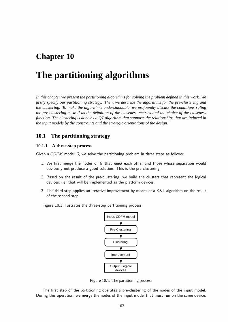
Chapter 10
The partitioning algorithms
In this chapter we present the partitioning algorithms for solving the problem defined in this work. Wefirstly specify our partitioning strategy. Then, we describe the algorithms forthe pre-clustering andthe clustering. To make the algorithms understandable, we profoundly discuss the conditions rulingthe pre-clustering as well as the definition of the closeness metrics and the choice of the closenessfunction. The clustering is done by a QT algorithm that supports the relationships that are induced inthe input models by the constraints and the strategic orientations of the design.
10.1 The partitioning strategy
10.1.1 A three-step process
Given a CDFM model G, we solve the partitioning problem in three steps as follows:
1. We first merge the nodes of G that need each other and those whose separation wouldobviously not produce a good solution. This is the pre-clustering.
2. Based on the result of the pre-clustering, we build the clusters that represent the logicaldevices, i.e. that will be implemented as the platform devices.
3. The third step applies an iterative improvement by means of a K&L algorithm on the resultof the second step.
Figure 10.1 illustrates the three-step partitioning process.
Pre-Clustering
Input: CDFM model
Clustering
Improvement
Output: Logical devices
Figure 10.1: The partitioning process
The first step of the partitioning operates a pre-clustering of the nodes of the input model.During this operation, we merge the nodes of the input model that must run on the same device.
103

104 CHAPTER 10. THE PARTITIONING ALGORITHMS
To do that, we solve the relationships that induce a dependency between the nodes of the inputCDFM model. These relationships are specified by means of needs and excludes relations betweenthe nodes and between the tokens of the input model. As needs and excludes relations are formallydefined, they can be treated automatically as well as manually. The result of this operation is agraph of atomic modules (called super-modules) that will be assigned each unbroken to a deviceof the system and a set of messages. At the end of this operation, there are no further needsrelations in the graph of super-modules.
The second step of the partitioning is a constraints-oriented clustering. We operate a bottom-up clustering on the result of the first step of the partitioning. In this operation, we progressivelymerge the modules that are related according to the strength of their relation. The result of thisstep of the partitioning is a graph of clusters, each representing a logical device of the system. Aswe assume that the number of devices that will be implemented on the platform is not pre-defined,we have two possibilities to terminate the clustering: Firstly, the size of each device (upper boundcapacity) is known. Secondly, the maximum number of messages allocated to a device is known.These are the most probable constellations of the architectural design of AES.
The third step of the partitioning deals with the improvement of the result of the second step.Two super modules that are assigned to different devices will communicate by passing signalsthrough the bus. A frame can contain several signals produced by several super modules thatare assigned to the same device (cf. frames multiplexing in section 11.1.4). At this step of thepartitioning process, we assign the signals to the frames, then we optimize progressively theseassignments. Here, we can redefine the partitioning problem as follows:
Problem formulation 10.1 (Improvement). : Assuming that the functioning of the system is guar-anteed by its actual configuration under the given constraints, what is thegain in terms of frameseconomy if we change this architecture?
10.1.2 Definitions of terms
We now introduce the following terms that will be used to describe the partitioning.
Definition 10.1(Configuration). At each time in the partitioning process, the configuration of aCDFMmodel is the actual composition of its nodes and the characteristics of its edges. A configuration ischanged by a clustering operation.
Definition 10.2 (Partition). A partition P of a CDFM model is a configurationP1,P2, . . . ,Pn of thegiven CDFM model where each clusterPi represents the functionality of a device. A partition is agraph of clusters.
Definition 10.3 (Part). Each nodePi of a partitionP is called a part ofP. A part is a cluster ofcomponents that represents a logical device. Per analogy with the real system, we may also say part ofthe system or device.
Definition 10.4 (Clustering). The clustering is the process of building hierarchical modules (i.e. clus-ters) from the nodes of aCDFM model.
Definition 10.5 (Partitioning). The partitioning is the process of building a partition, i.e. the processof grouping the system’s components (i.e. the nodes of aCDFM model) to build parts.
Definition 10.6 (Membership). A modulem1 is a member of a bigger modulem2 if m1 is embeddedin m2, i.e. the functionality ofm1 is a part of the functionality ofm2.The notationm2+m1 means thatm2 andm1 become members of the same cluster.The notationm2-m1 means thatm1 looses its membership inm2.A token Tk
i j is a member of a messageMqi if the significance ofMq
i looses its plenitude whenTki j is
extracted fromMqi .
Definition 10.7(Sub-module). A modulem1 is a sub-module of a modulem2 if m1 is a member ofm2.
10.2. THE PRE-CLUSTERING 105
10.1.3 The main procedure
The main procedure described in algorithm 1 implements the three-step partitioning process. Itinputs a CDFM model G and outputs the final configuration of the logical architecture of thesystem, i.e. the best partition.
Algorithm 1 PROCEDURE Partitioning(G: CDFM)1: SuperModules:= Pre-Clustering(G);//* Builds the graph of super-modules by solving needs and
excludes relationships2: InitialConfig:= Clustering(SuperModules);//* Partitions the graph of super-modules and returns
the initial configuration of the system3: FinalConfig:= Improvement(InitialConfig);//* Improves the initial configuration of the system and
returns the final configuration, i.e. the best partition4: return FinalConfig;//* Final definition of the logical devices and the frames
10.2 The pre-clustering
10.2.1 Definition
The procedure ”Pre-clustering” must find the pairs of nodes (vi ,v j) of the input CDFM model Gthat must be merged and build the super-modules with them. We first introduce the followingrules to solving the needs and the excludes relations.
Definition 10.8(needsandexcludes). For each two nodesvi andv j , the notations ”vi needsv j ” and ”vi
excludesv j ” mean that there is a needs resp. an excludes relation betweenvi andv j while needs(vi ,v j)andexcludes(vi ,v j) mean that the two nodes can effectively be clutched resp. must be separated. Thusfor each two nodesvi andv j of aCDFM model,
• IF needs(vi ,v j) THEN vi andv j must run on the same device and thus must be merged to forma super-module.
• IF excludes(vi ,v j) THEN vi andv j may never run on the same device.
All the relations guiding the pre-clustering can be specified in terms of needs and excludesrelations between the nodes of G. The pre-clustering thus finally aims at merging the needs-relatedcomponents. Excludes relations will be treated later in the partitioning process, always whennecessary. The following properties of the needs and excludes relationships state the rules thatguide the pre-clustering. Note that these properties are identical for both the nodes and the tokens.
The needs relation is:
• reflexive, i.e. for each vi , vi needs vi AND needs(vi ,vi).
• transitive, i.e. IF needs(vi ,v j) AND needs(v j ,vk) THEN needs(vi ,vk).Similarly, IF vi needs v j AND v j needs vk THEN vi needs vk.
• not symmetric (per agreement), i.e. IF needs(vi ,v j) THEN not obligatorily needs(v j ,vi).Similarly, IF vi needs v j THEN not obligatory v j needs vi
and the excludes relation is:
• not reflexive, i.e. for each vi , ¬(vi excludes v j) AND ¬excludes(vi ,vi).
• not transitive, i.e. IF excludes(vi ,v j) AND excludes(v j ,vk) THEN not obligatorily excludes(vi ,vk).Similarly, IF vi excludes v j AND v j excludes vk THEN not necessarily vi excludes vk.

106 CHAPTER 10. THE PARTITIONING ALGORITHMS
• but symmetric (per definition), i.e. IF excludes(vi ,v j) THEN excludes(v j ,vi).Also, IF vi excludes v j THEN v j excludes vi .
The needs and excludes relations between the tokens induce some needs and excludes rela-tionships between the nodes producing these tokens. Given two tokens Tk
il and Tnjm ∈ Ω,
• IF Tkil needs Tn
jm THEN vi needs v j
• But IF Tkil excludes Tn
jm THEN vi and v j don’t care.
However, when solving the needs and excludes relations, some conflicts can arise, for example,when a single node is involved in several needs and excludes relationships or when the relationshipsbetween the nodes are conflicting with the relations between the tokens. In the following, weexamine these conflicting situations. The needs relations are intended to augment the quality ofthe partition (i.e. performance and cost). Passing over a needs relation can reduce the chance tofind the optimal system architecture, but it will not be dramatic for the functioning of the system.In contrast, ignoring an excludes relation can cause serious faults in the system’s functioning. Sinceour primary objective is to build well-functioning systems, we agree that the excludes relationshipis stronger than the needs relationship, i.e. for each two nodes vi and v j of G, given two tokensTk
il and Tnjm ∈ Ω,
• IF vi needs v j AND vi excludes v j THEN excludes(vi ,v j).
• IF vi needs v j AND v j excludes vi THEN excludes(vi ,v j).
• IF a sub-module of vi excludes a sub-module of v j THEN excludes(vi ,v j) (and consequentlyexcludes(v j ,vi)).
• IF needs(Tkil , Tn
jm) THEN vi needs v j AND (Tkil and Tn
jm) build a message.
• But IF excludes(Tkil , Tn
jm) THEN vi and v j don’t care.
Proposition 10.1(needs). needs(vi ,v j) == TRUE if and only if there is at least one sub-module ofvi that needs a sub-module ofv j AND there is no sub-module ofvi that excludes a sub-module ofv j
AND no sub-module ofv j excludes a sub-module ofvi .
10.2.2 The pre-clustering algorithm
The procedure ”Pre-Clustering” finally runs the following algorithm:In procedure 2, the instruction ”Actualize the edges connecting the new SuperModules” deter-
mines the connections of the new super modules, i.e. the edges connecting a new super modulewith any other node and the corresponding weights (see definition 10.11 and figure 10.2). Thefollowing definitions specify the process of actualizing the edges of the graph of super modules.
Definition 10.9 (Neighborhood of a node). : Given a nodevi of G, the neighborhood ofvi , calledNeighborhood(vi) is the set of the nodes that are directly related withvi , i.e. Neighborhood(vi) = set ofthe nodesv j , so that there is an edgeei j in G.
Definition 10.10(Neighborhood of a super module). : Given a super modulevi with sub-modulesvik,k∈ N, Neighborhood(vi) =
⋃
k Neighborhood(vik)
Definition 10.11 (Weight of a super edge). : If vi is a super module with sub-modulesvik, then foreachv j ∈ Neighborhood(vi),
Ti j =⋃
k Tik j andTji =⋃
k Tjik
thusei j .T =⋃
k eik j .T

10.3. THE CLUSTERING 107
Algorithm 2 PROCEDURE Pre-Clustering(G: CDFM)1: nbModules :=|SetO f SuperModules|; //* SetOfSuperModules is the set of the nodes of G2: k:= nbModules + 1;//* temporary index for the new modules3: for all vi , v j in SetOfSuperModulesdo4: if needs(vi ,v j) then5: vk := vi + v j ; //* merge them into a new hierarchical module vk following property 10.16: SetOfSuperModules:= (SetOfSuperModules -vi - v j ) ∪ vk;7: nbModules:= nbModules - 1;8: k:=k+1;9: Actualize the edges connecting the new SuperModules;//* Super-edges following definition
10.1110: end if11: end for12: Actualize the indexes of the SuperModules;//* Allocate the indexes from 1 to nbModules13: return SuperModules;//* Graph of super-modules with actualized edges
(a) Modules and edges
v1
v2v3
v4
v6
v7
v5
T115
T215
T125
T135
T236T1
36
T227T1
27 T327
T147
(b) A super module with the super-edges
v1
v2v3
v4
v6
v7
v5
T115
T215
T125
T135
T236T1
36
T227T1
27 T327T1
47
Figure 10.2: The super graph
10.3 The clustering
10.3.1 Closeness metrics
The procedure ”Clustering” implements the second step of the partitioning. It clusters the nodesof the graph of super modules in order to build the logical devices. To do this, it merges closelyrelated modules in order to implement them on the same device. Concretely, the problem to solvehere is to find a clustering that minimizes the data exchange on the bus, i.e. the inter-clusterscommunication, and that at the same time meets the design constraints and the other optimalityconcerns such as maximizing the HW sharing, optimizing the grouping of the components followingthe strategic requirements like the level of safety, the mission- or the business-criticality, the sourceof procurement, the production issues, the potential level of reuse, the rhythm of changing, thetarget of the procured service, etc. For instance, two modules will be closely-related if there is noexcludes relationship between them and they are related with each other in some way, for exampleif:
• they can share resources (i.e. HW and frames),
• they have common accesses,
• they communicate with each other,
• they underlie a relation given by the strategic orientation of the design
In order to determine the closeness between two modules, all the involved closeness factorsmust be quantified and combined with each other. The first step in solving this multi-objectivesoptimization problem is to formalize the objectives. This step may yield a set of closeness functions.

108 CHAPTER 10. THE PARTITIONING ALGORITHMS
A closeness function is defined by a closeness metric that can measure and compare the strength ofa given relation between two modules. The higher the closeness between two modules, the closerthe two modules are related. The closeness metrics must thus reflect the closeness factors and theobjectives of the design.
The resource sharing metric: The potential that two modules have to share a given hardwareunit is often considered as a closeness factor in the design of embedded systems [116]. However,a satisfactory HW (processing unit, e.g. ASIC) sharing metric cannot be extracted from our inputmodel because of its high resolution. Thereto, as the components of the HW devices of the platformare not allocated, it will be particularly difficult to analyze the potentiality of two components toshare a given HW. Furthermore, the hardware sharing is obviously not useful in our case, since weare concerned with the mapping of the modules on the logical devices (i.e. Partitioning 1) ratherthan with the deployment of the tasks and processes (Partitioning 2). However, if known, the HWsharing can be considered as a strategic decision that is taken before the partitioning, specifiedin the input model, e.g. in the form of needs, and used in the pre-clustering to build the supermodules. Therefore, the HW sharing metric will certainly not induce any substantial benefit in thequality of the partitioning (i.e. in the mapping).
The frames sharing metric: The frames sharing metric measures the potential of two modulesto share frames. The likelihood to share frames is determined by the number of tokens that areproduced in the same range of time by two modules. Modules that produce a high number oftokens within the same range of time are more likely to share frames. Thus, following the framessharing metric, the higher the number of tokens produced within the same range of time, the closerthe producing modules are related. If vi .datesis the set of ranges of time within which the modulevi produces its tokens, the frames sharing metric can be defined as:
FrameSharing(vi ,v j) = |vi .dates∩v j .dates| (10.1)
The common accesses metric: Grouping two modules that have a great number of commonaccesses would probably improve the quality of the communication by reducing the number offrames needed for the inter-components communication. Assuming that each module is its ownneighbor, the common neighborhood of two modules vi and v j defines the number of modules thataccess, i.e. exchange tokens with, both vi and v j . The common accesses metric is defined as:
CommonAccesses(vi ,v j) = |Neighborhood(vi)∩Neighborhood(v j)|
The communication metric: Grouping two modules that heavily communicate with each otherwill obviously increase the performance of the communication. The communication metric mea-sures the magnitude of the communication between two modules. This is determined by theamount of data exchanged between the two modules. The simplest and most usual way to mea-sure the communication between two modules is to count the number of bits exchanged betweenthem, i.e.
Communication(vi ,v j) = ∑k Tki j .res×Tk
i j . f req + ∑k Tkji .res×Tk
ji . f req.In this case, the modules exchanging the highest number of bits are the closest. But, in
our case, two components that are assigned to different devices will communicate by exchangingsignals over the bus. The communication metric must measure the impact of the separation of twomodules on the occupation of the bus. This depends on the number of frames that are sent on thebus and the length of each of them. Each short token (i.e. resolution≤ max f rameL) can fit into aframe. A long token will be fragmented into the corresponding number of signals that can fit eachinto a frame. Short frames occupy the bus differently, depending on their length. The following
10.3. THE CLUSTERING 109
example illustrates the expressiveness of this metric. Suppose four modules v1, v2, v3 and v4 of aCDFM model. Within an activation time of the system, v1 exchanges a token of 20 bits 10 timeswith v2 (interface e12), a token of 100 bits 3 times with v3 (interface e13) and a token of 112 bits3 times with v4 (interface e14). Considering the number of bits exchanged, Communication(v1,v3)= 100×3 = 300bits is greater than Communication(v1,v2) = 20×10 = 200bits, meaning thatv1 is closer to v3 than to v2. But considering the number of signals (assuming that max f rameL=8 Bytes), e12 would produce 10 signals while e13 produces 2×3 = 6 signals, meaning that v1 iscloser to v2 than to v3.
These two conclusions are contradictory. But the number of signals produced by an interfaceclearly better captures the impact of the merging or the separation of two modules on the busoccupation than the number of bits exchanged between them. Now, e14 also produces 2×3 = 6signals. But these signals are longer than the signals produced by the interface e13, what meansthat the medium would be more occupied by e14 than by e13 and consequently v1 is closer to v4
than to v3, although both interfaces produce each 6 signals. Thus, the closeness of two modulesdoes not depend only on the number of signals produced by their interface, but also on the lengthof the signals. However, the length of the signals makes the difference only when two interfacesproduce the same number of signals. To get a feeling of the impact caused by the length of asignal on the load of the medium, suppose that the bit-time on a given medium is tb. The bit-timeis the latency resulting from the propagation of a bit on the medium, i.e. the diffusion time ofone bit. In a CAN network, the bit-time depends on the operating rate of the network and thelength of the bus. Note that the bit-time is different from the transmission time of a bit. Thelatter is made up by the delay caused by the medium driver, the time spent in the CAN-controllerand the CAN-transceiver of the receiver device, and the diffusion time of the bit on the specificactual medium. Since each frame contains the user data that is of variable length and a relativelyconstant number (i.e. 47) of framing bits, we will consider in the following only the delay inducedby the user data for each frame. In a serial transmission method, the time that is necessary for thediffusion of a signal s of length signalL (the framing bits are not included) will be approximately:
t(s) = signalL∗ tb
and the total medium occupation time induced by the throughput of an interface ei j is equal to:
t(ei j ) = ∑s∈ei jt(s)∗s. f req
Thus, the higher t(ei j ), the closer the modules i and j. This formulation of the closeness resultsagain in the number of bits exchanged between two modules. However, it only makes sense if it isapplied on two comparable interfaces that produce the same number of signals.
In conclusion, the number of signals is by far the most efficient communication metric in aCDFM model. The higher the number of signals produced by an interface, the closer the twomodules. When two interfaces produce the same number of signals, the communication loadinduced by each of them can be used to make the difference. The combination of these twometrics allows to fairly compare the magnitude of the communication between the modules of aCDFM model. The communication metric can thus be defined as follows:
Communication(vi ,v j) = nbSignals(ei j )
= ∑k
nbSignals(Tki j )+∑
k
nbSignals(Tkji )
To compare two interfaces that have the same number of signals,
Communication(vi ,v j) = t(ei j )

110 CHAPTER 10. THE PARTITIONING ALGORITHMS
The constraints and strategic relationships metric: The closeness factors between the modulesinduced by the constraints on the communication and the strategic factors must also be quantified.These factors tend to change constantly and depend on unpredictable events. They cannot beaccurately formalized. However, following their importance, these closeness factors can be classifiedobjectively. For example, if a constraint or a strategic factor induces strength relationships betweenthe modules, it can be modeled by the means of needs and excludes relations and then solved duringthe pre-clustering. Else, the designer will quantify these factors following the level of accuracy oftheir demand for achievement. In fact, the strategic closeness factors as well as the non-functionalconstraints can be classified in ”must be” and different degrees of ”will be nice” closeness levelswhereas ”must be” relationships can be modeled as needs and excludes relations. The degree ofimportance of a closeness factor in the ”will be nice” class can be easily fixed exactly as the levelof priority of a message or a task. In practice, an integer is sufficient to model such a rankingas the level of nicety of these factors can be evaluated so that each becomes the desired weightcompared to the other factors. Thus, if a closeness factor is very important, it receives a highcloseness value that will prevent the partitioning algorithm to ignore it. Otherwise, it is assigned acloseness value that can make the clustering difficult or easy depending on its level of nicety. Wecan thus assign a tag to each relation induced by a strategic factor that corresponds to its level ofnicety. Each tag is an integer.
Relationships(vi ,v j) = ∑ tags(ei j )
= Tag(ei j )
10.3.2 The closeness function
Because the closeness factors are disparate and mostly competing, some trade-offs must be done.Making trade-offs means that there is no unique solution. We thus have to find the best possiblecloseness function or the closeness functions that are achieved by acceptable trade-offs between thecloseness factors and choose the optimal one. In this case, the optimality is not absolute, since theoptimal solution refers to a point in the set of the optimal solutions, i.e. a Pareto optimal point.Anyway, deciding which trade-offs are acceptable might be subject to laborious investigations. Themost intuitive approaches to make trade-offs include the weighting of the factors, the hierarchicaloptimization (also multilevel programming) method and the goal programming method. Whenproceeding by weighting the factors, the closeness functions are positively weighted and a singlescalar closeness function is obtained by adding the weighted closeness functions. The weightingcoefficients are then varied to yield a set of feasible optima, e.g. the Pareto optimal set. It is up tothe user to choose appropriate weights to generate various points in the Pareto set. The weightingstrategy is a standard technique for solving multi-objective optimization problems. But, typicallyfor linear functions, the relationship between the weights and the Pareto curve is generally so thata uniform spread of weights rarely produces a uniform spread of points in the Pareto set. Often,all the points found are clustered in certain parts of the Pareto set with no point in the interestingmiddle part of the set, providing thereby little insight into the shape of the trade-off curve. Ingeneral, it is difficult for the user to find the optimal vector of weights. However, the closenessfactors of our problem show that we can probably achieve a very simple closeness function with acombination of the closeness metrics.
The hierarchical optimization method aims at finding just one optimal point in oppositionto the entire Pareto set. In this method, the closeness factors are firstly ordered following theirimportance. Each closeness function is then optimized individually, subject to a constraint thatdoes not allow its minimum to exceed a prescribed fraction of the minimum of the previous function.The method proceeds recursively until all the objectives have been optimized on successively smallersets of possible optimal solutions. This method is also called multilevel programming. Multilevelprogramming is a useful approach if the hierarchical order among the objectives is important andthe designer is not interested in the continuous trade-offs among the functions. However, the
10.3. THE CLUSTERING 111
problem becomes very tightly constrained in the lower steps down in the hierarchy and oftenbecomes numerically infeasible, so that the less important factors have no influence on the finalresult. Our problem easily fits in this method as the closeness factors can be clearly ordered.Furthermore, ignoring the less important closeness factors (resource sharing and common accessesmetrics) is not dramatic at all.
The goal programming method aims at minimizing the deviation from the target constraints. Inthis approach, we optimize one factor while constraining the remaining factors to be less than thegiven target values. The user chooses weighting factors to rank the goals in order of importance.Finally a single objective function is written as the minimization of the deviations from the abovestated goals. This is perhaps the most well-known method for solving multi-objectives optimizationproblems. However, it is not always easy to choose the appropriate goals and the good weights forthe constraints. For these reasons the goal programming method is not a viable solution for ourproblem.
Consider the following function: Closeness(vi ,v j) = ∑k αkClosenessMetrick(vi ,v j) where theweights αk correspond to the relative importance of the closeness factors (i.e. resource sharing,frame sharing, common accesses, relationships, constraints, communication). We now examinethe weighting of the closeness factors: In a CAN network, the frames are owned by the sender, notby the receiver. Each frame can have several receivers but only one sender. There is therefore noobvious advantage to cluster the modules that have common accesses. In opposition, clusteringthe modules that can share frames can be beneficial. But before doing this, it is necessary to reducethe inter-device communication load as described in section 11.1.5. The reason of the uselessnessof the resource sharing metric have been discussed above. In the end, the communication metricand the strategic relationships are the most useful metrics for the clustering. As the tags areassigned to the relationships in a way that they correspond to the weight they need, we can definethe closeness function as follows:
Closeness(vi ,v j) = Communication(vi ,v j)+Relationships(vi ,v j)
= nbSignals(ei j )+Tag(ei j )
= ∑k
nbSignals(Tki j )+∑
k
nbSignals(Tkji )+Tag(ei j )
10.3.3 The QT clustering algorithm
The clustering deals with the multi-objective optimization problem identified above. The problemis to cluster the modules whose communication, if separated, might highly occupy the bus and toconjointly satisfy the given strategic concerns of the design. The capacities of the available devicesare given. Using the above defined closeness function, we can easily extract the closeness valuesfrom the input model (i.e. the CFDM graph of super modules) and display them for example in acloseness matrix where excludes relations can be represented with a negative value, e.g. −1. Theprocedure ”Clustering” finally runs the algorithm 4. It uses the procedure ”InitialConfiguration”described in algorithm 3 to solve the excludes relations.
This clustering procedure assures that whenever two nodes underlie an excludes relation, theywill not be assigned to the same cluster. At the beginning, all the nodes that can definitely notbelong together are set as starting points for different clusters (in algorithm 3). These clustersare then completed before checking if new clusters are necessary (in algorithm 4). The remainingmodules are thereafter clustered following an agglomerative clustering technique by which theclosest pairs are merged. After the completion of the initial clusters, the working principle of theprocedure can be resumed as: Whenever a cluster is initialized, grow it up until the given limitbefore the construction of the next cluster begins. This is a QT algorithm. At each time, theactual configuration of the partitioning is made of the remaining modules (i.e. super modules)that are not yet assigned to a part and the parts that are not yet completed. A module can beassigned to a part only if it is the closest for which the assignment is feasible. An assignment is

112 CHAPTER 10. THE PARTITIONING ALGORITHMS
Algorithm 3 PROCEDURE InitialConfiguration(SuperModules)1: InitialConfig:= SuperModules;//* Initial set of parts2: repeat3: Traverse the set of super-modules;4: until The first pair(vi ,v j) with excludes(vi ,v j) is found;5: Setvi andv j to be 2 different initial partsPi andPj of the partition;6: RestOfSuperModules:= SuperModules -
vi ,v j
;7: InitialConfig:=RestOfSuperModules∪
Pi ,Pj
;8: for all vl ∈ RestOfSuperModulesdo9: for all elementsvm that are already in a starting partitiondo
10: if excludes(vl ,vm) then //* v l excludes all the existing parts11: Setvl to be another initial partPl ;12: RestOfSuperModules:= RestOfSuperModules -vl;13: InitialConfig:= InitialConfig∪ Pl ;14: end if;15: end for;16: end for;17: return InitialConfig; //* The graph of the first initial clusters and the remaining super modules
Algorithm 4 PROCEDURE Clustering(SuperModules)1: Initialize CompletedParts:=; //* Full clusters2: Run InitialConfiguration(SuperModules);//* Outputs the initial parts and the remaining super
modules3: repeat4: Find the closest pair(vi ,Pj) that is not constrained by an excludes relationship;//* Best next
assignment5: if Pj can aggregatevi then //* Content of Pj + vi ≤ Capacity of Pj6: Assignvi to Pj and deletevi from RestOfSuperModules;7: else//* Content of Pj + vi > Capacity of Pj but CAUTION! Pj is possibly not full8: CompletedParts:= CompletedParts∪ Pj ;9: InitialConfig:= InitialConfig -Pj ;
10: end if11: until InitialConfig==; //* The initial parts found by ”InitialConfig” are all completed12: repeat13: if RestOfSuperModules6= then14: Choose acentral elementvi of RestOfSuperModules and set it to be an initial partPi in
InitialConfig;15: Assign the closest modulev j of RestOfSuperModules toPi , Then the next closest, and so on
UNTIL the size ofPi meets its limit;16: CompletedParts:= CompletedParts∪ Pi ;17: end if18: until no remaining RestOfSuperModules;19: InitialConfig:= CompletedParts;20: return InitialConfig;

10.3. THE CLUSTERING 113
feasible if the behavior of the part and the behavior of the system are not compromised by theassignment. Whenever a module is assigned to a part, the closeness matrix is actualized.
The QT clustering procedure terminates successfully if each module is assigned to at leastone part. It behaves greedily for both the initialization of the parts and their growing, i.e. nobacktracking. This one-shot, one-dead strategy leads perforce to a hard, i.e. exclusive partition-ing. However, the procedure can be easily adapted to achieve fuzzy, overlapping and redundantpartitioning, for example by enabling the concerned modules to be assigned to the closest, thenext closest part and so on, or by correspondingly modifying the assignment process, for exampleby marking instead of deleting a module from the set of free modules after its assignment to acluster. Redundant partitioning is needed for example if redundant implementation of some mod-ules is required, e.g. for safety and reliability reasons. Modules that must be partitioned fuzzilymay have a degree of membership for each potential target cluster. The degree of membership isfor example a number between 0 and 1 indicating the probability that the module will be assignedto the corresponding cluster. Fuzzy partitioning is a realistic partitioning option at the level ofproduct-lines design where the mappings might change from a product variant to another onefollowing some stochastic rules. These features can be easily implemented in an extended versionof our algorithm.
10.3.4 Conclusion
We follow a three-step partitioning process beginning with the pre-clustering that solves the needsrelationships and merges the needs-related components. Then, we use a powerful closeness functionto proceed the clustering of the nodes of the graph that has been produced by the pre-clustering.The closeness of two given nodes of the super-graph is measured by a combination of the magnitudeof the communication with the relations induced by the constraints and the strategic relationshipsbetween the modules of the system under design. At this step, we use a QT algorithm that is ableto solve the excludes relationships. The algorithm designed here assumes that the capacities of theavailable devices are given. This information is used as the threshold. The clustering algorithmalways yields a feasible partition of the input CDFM model, i.e. in the sense of the capacities ofthe allocated devices. But a further important question remains open: Is this the best algorithmor at least is this a good one? This question will be answered in the next chapters.

114 CHAPTER 10. THE PARTITIONING ALGORITHMS

Chapter 11
Evaluating and improving a partition
The purpose of this chapter is to explain the method by which we improve a partition. Before improvinga partition, we must evaluate it. Then we process a perturbation of its configuration and we evaluatethe result. This is done a few times. At the end, we take the best solution. To achieve this process, wemust define the cost function, i.e. the metric by which the value of a partition willbe determined. Asthe optimizing of the usage of the consumption of communication frames is the primary declared goalof the partitioning process followed in this work, we begin this chapter by introducing the CAN pro-tocol as the example for the frames-oriented communication protocols. Frames-oriented automotivecommunication protocols include LIN, FlexRay, CAN, MOST, etc. The CANis the most prominent ofthis class of communication protocols in the automotive domain. We hereby discuss the frames multi-plexing techniques and their relations with the partitioning. This discussion alsoincludes an outlineof the requirements for the multiplexing of the frames, the constraints that govern the multiplexing andthe rules that guarantee a good partitioning in relation with the multiplexing of frames. Then, as thecost function is defined as a bin packing problem, we revise the state-of-the-art in the resolution of binpacking problems in order to find out if there exists a solution that is adequate for our problem. TheFFD that is investigated as the best solution that fits to our purpose is used to design the algorithmimplementing the cost function. We finally present our improvement algorithm. It is an adaption of theK&L partitioning approach.
11.1 The CAN: A frame-oriented communication protocol
11.1.1 Organization of a CAN network
CAN (Control Area Network) is a frames-oriented event-triggered communication concept used inautomotive systems. The CAN uses a synchronous serial bit transmission method that affords theeconomizing of the communication bandwidth, i.e. an information is transmitted as a sequence ofbits in a frame and when necessary, the synchronization between sender and receiver is done atthe beginning of the frame, rather than for each bit as it would be the case in an asynchronoustransmission mode. CAN is a multi-master network based on the carrier-sense multiple-accessmethod with collision detection (CSMA/CD). Thus, a CAN network enjoys a flat organization inwhich all the nodes are equal in rights. Each node can place a frame on the medium as soonas it is ready. When a collision is detected, the node sending the frame with the highest prioritywins the competition. The priority of a frame is coded in its identifier (ID). The lower the ID ofa frame, the higher its priority, i.e. the frame with the smallest ID value has the highest priority.Collisions are resolved through a bitwise comparison of the IDs of the competing frames. Oncea node wins the competition, it takes the control of the medium and finishes to send its framebefore releasing. Furthermore, to each frame, a minimal time interval (i.e. the Inhibit-Time) canbe assigned between two successive medium accesses (see the CMS-CAN frame Specification) thatensures that each frame will have the possibility to be placed on the medium independently of itspriority and no node will be able to confiscate the medium for too long time.
115

116 CHAPTER 11. EVALUATING AND IMPROVING A PARTITION
Each CAN frame that is set on the medium is broadcast in the whole network and can beread by every device that is ready. Excepting some particular types of frames such as the networkmanagement (NM) and the diagnosis frames for which the receiver’s address is introduced in thedata part of the frames, the addressees of a CAN frame, i.e. those that are interested in thecontents of the frame, are not coded in the frame. A device identifies a frame that is addressedto it only if it knows the ID of this frame. This is, it has been preprogrammed to receive theframe. CAN networks are generally implemented on linear two-wire buses, but the CAN protocolcan be implemented as star topologies, on optic fiber or on single-wire buses as actually done forthe comfort functions in AES (e.g. see section 1.1).
11.1.2 CAN frames
Following the CAN protocol, four classes of frames, also called telegrams, can be identified in aCAN network:
• The data frames: These are the frames that transport the application data.
• The remote frames: These are the frames used for data request, i.e. they are used by a nodeto require an information from another node.
• The error frames: These are the frames that can be used to notify a functioning error (e.g.during sending or reading).
• The overload frames: These are the frames that can be used by a node to request an extradelay between two consecutive frames.
The error frames are not used by the application, but rather by the basic software. Equally,the overload frames are not used by the application, but rather by the CAN drivers. The remoteframes are formatted like the data frames as shown in figure 11.1 while the error and the overloadframes have different formats [46]. The most known CAN implementations (CAN-controllers) donot use the overload and the remote frames. The spacing of successive frames is realized throughthe placement of ”intermission” fields between two frames that impose a respectable inter-framespace. Data requests are achieved with data frames. The data frames are thus the only interestingframes for our purpose.
Depending on their role, there are the following types of data frames in a CAN system:
• Diagnosis frames
• Network management frames
• Data request frames
• Standard frames
The diagnosis frames are received by all the devices in the system including the diagnosisgateways. The network management frames are received by all the networked devices. The datarequest frames are received only by the devices that can send the requested information. Thestandard frames are received only by the devices that need the sent information. In this work, weare interested only in the transfer of the data (i.e. tokens) of the application software, thus in thestandard data frames that can be used to send or request application-relevant information.
11.1.3 Format of a standard CAN data frame
We can distinguish three versions of the CAN protocol: The low-level CAN (ISO 11519) runningup to 125 kbps, the so-called standard CAN (2.0A; ISO 11898:1993) and the extended CAN (2.0B;ISO 11898:1995) both running up to 1Mbps. Following the CAN specification (ISO-WD 16845),

11.1. THE CAN: A FRAME-ORIENTED COMMUNICATION PROTOCOL 117
each frame has a unique identifier of 11 bits length in the ”Standard format” and 29 bits in theso-called ”Extended format”. In this work, we consider the standard format (i.e. IDE-bit = 1).The ID of a CAN frame, defined between 0 and 2047, clearly identifies the frame and the sender.As shown in figure 11.1, a standard CAN data frame is made up by 1 bit SOF (Start Of the Frame)+ 11 bits Identifier + 1 bit RTR (Remote Transmit Request) + 1 bit IDE (Identifier ExtensionBit) + 1 bit that is reserved for scalability + 4 bits for DLC (Data Length Code) + 0..8 bytes forUser Data + 15 bits CRC (Cyclic Redundancy Check) + 1 bit DEL (Delimiter) + 1 bit ACK + 1bit again DEL + 7 bits EOF (End Of Frame) + 3++ bits IFS (Inter Frame Space). The IFS hasat least three bits that are part of the frame. All additional bits that can appear in the IFS are notpart of the frame, but they are solely considered as separation bits.
IFSEOF
DE
L
AC
K
DE
L
CRC User DataDLC R
es.
RT
R
Identifier
SO
F
1 11 1 2 0..8 bytes4 15 1 1 71 3++
Figure 11.1: Format of a standard CAN data frame
The CRC contains the information needed to check the safety of the transmission, i.e. theintegrity of the frame, that is confirmed by setting the ACK (acknowledge) bit. The CRC has a1 bit delimiter (DEL). The IDE-bit, the scalability-bit and the DLC-bits build the Control Field ofa CAN frame. The IDE-bit indicates the format of the frame, i.e. value 1 for standard and 0 forextended format. The RTR-bit is used to distinguish a data frame (RTR = 1, i.e. dominant) froma remote frame (RTR = 0, i.e. recessive). All the bits used in a CAN frame around the user data(e.g. the 47 heading and queue bits used in the best case, i.e. with the minimum -3 bits- EOF instandard CAN frames) will be called in the remainder of this work ”Framing Bits”.
11.1.4 Frames multiplexing
In a CAN network, each piece of information exchanged between two functional components of thesystem that are located on different devices is transported by a frame. After the partitioning, eachdevice is assigned a given set of data frames, i.e. frames IDs, that must be sufficient to transferthe application’s data to the other devices. The application’s data of a device is the set of thetokens that are emitted by the corresponding logical device. For a device Pi of a partition P, thisset is given by the operator Tokens(Pi) that extracts all the tokens for which the source is Pi , i.e.
Tokens(Pi) :=
Tki j , f or each device j; k∈ N
The name, the ID, the DLC and the contents of the user data part of each frame are staticallypredefined. In complex systems like automotive systems, the number of tokens exchanged via thenetwork medium is generally more than the number of the frames that are available. For illustration,less than half of the total possible 2048 frames are available in the CAL (CAN Application Layer)DBT-Model, i.e. are free to be used for data transfer, and a large number of these frames isreserved for the system, the basic software services and other predefined messages like the networkmanagement and the diagnosis messages. Thus, it is not opportune to invest one frame for eachtoken. Even if we are provided sufficient frames, the bandwidth of the network is not unlimitedand the throughput in an AES network must be designed so that even by maximal load, there isstill room for the transmission of asynchronous messages, particularly in the case of event-triggeredcommunication systems.
As the number of frames is limited, the designer must optimize their usage. An effective way tooptimize the usage of frames is to make use of frames multiplexing [46], i.e. under some conditionsseveral pieces of information can be joined together in a single frame in a way that increases theeconomy of the frames. A frame to which more than one piece of information is assigned is a

118 CHAPTER 11. EVALUATING AND IMPROVING A PARTITION
multiplexed frame. A device receiving a multiplexed frame must de-multiplex it to extract theinformation that is addressed to it. In order to enable the frame de-multiplexing, a part of the userdata field (e.g. the first byte of the user data field in CAN) of a multiplexed frame is used to codethe sub-identifiers of the sub-frames, i.e. the IDs of the different entities of information containedin the frame. We now introduce the following definitions for the terms that will be used in thecontext of frame multiplexing. The relationships between these terms are illustrated in figure 11.2.
Definition 11.1 (Data object). A data object is a piece of user information exchanged between twofunctional components.
Definition 11.2 (Token). A token is the logical representation of a data object in the context of syn-thesis models.
Definition 11.3 (Signal). A signal is an atomic, i.e. an elementary piece of user information that issent by a device to another one. Each signal represents a token or a fraction of a token. For example,a token that fits in a frame constitutes one signal. A token that is longer than a frame can be split inseveral signals. Thus, a multiplexed frame contains several signals.
Definition 11.4 (Packet). A packet is a set of signals that are sent together within a frame, i.e. asa block of sequential signals. A multiplexed frame contains exactly one packet of signals, whereaseach signal constitutes a sub-frame. The sum of the signals transported within a frame determines thepayload of this frame.
Definition 11.5(Message). A message is a meaningful and complete piece of information. A messagemight be made of one or several tokens. For example, some tokens are constrained to be always shippedtogether. This relationship is modeled inCDFM models by means ofneedsrelations. The tokens thatneedeach other are bundled within a message. If a token isneeds-related with several other tokens,then it will be redundantly instantiated in each message containing an associated token. The length ofa messagemessLis defined as the sum of the resolutions of the constituting tokens.
Definition 11.6 (Sub-frame). A sub-frame is a distinguishable and separable part of a multiplexedframe. This concept aims at providing an ID to each signal within a multiplexed frame. From the pointof view of a multiplexed frame, these IDs are sub-IDs. A sub-frame is thus made of one signal and thecorresponding sub-ID. Note that the sub-identification of frames is not recursive, i.e. sub-frames donot incorporate sub-IDs, since each sub-frame contains exactly one signal.
Definition 11.7(Frame). A frame is a block of information that is transferred from a sender device tothe receivers. A frame is made up of one signal or when multiplexed, it contains several sub-frames.The concept of frame is analog to the concept of slots known in some protocols like FlexRay or MOST.
Frame * 1..*Sub-Frame Packet Signal1 10..1 1..*
1if 0 sub-frame1..*
MessageToken
1
1..* 1..*
1..*is transmitted as
Data object1 1
is a
Figure 11.2: Semantical relationships between the concepts for the frames multiplexing
Another multiplexing technique allows the variable occupation of some positions within a mul-tiplexed frame. For example, different signals can rotatively occupy the same position in a givenframe. This multiplexing technique is used for example when a periodic signal can share a framewith other signals, but at different sending times of the frame, different signals are available thatcan occupy the free positions. When this multiplexing technique is used, a switch is used to identify
11.1. THE CAN: A FRAME-ORIENTED COMMUNICATION PROTOCOL 119
the signal that actually occupies the varying position in the frame. A switch is a bit field within theuser data field of a varying multiplexed frame that indicates the signal that actually occupies thecorresponding varying position so that depending on its actual runtime value, a device receivingthe frame knows which signal is actually occupying the corresponding position. Both the values ofthe sub-frames and the switches are assigned statically during the system design.
11.1.5 Relations with the partitioning
The frames multiplexing itself is a signal partitioning problem. Actually, the frames are assigned tothe network nodes based only on the experience and the feeling of the designer. The assignmentof the signals to the allocated frames is done per hand, based on approximative calculations andpuzzles reasoning. Inexperienced designers cannot expect to find optimal solutions in a relativeshort time. Even experimented designers cannot verify the optimality of their solutions, althoughthere is a need of optimal system architectures and design time saving. Sustaining the framesmultiplexing through CAD is obviously necessary to allow AES system architects to explore newsystem architectures. CAD-based frames multiplexing will promote the evolution in the qualityof AES architectures and enable savings in the design time of systems that are based on frames-oriented protocols. Since we make benefits if we optimally occupy the user data field of eachframe, we will provide efficient solutions for the frames multiplexing problem if we are able to solvethe two following sub-problems:
1. Minimize the number of tokens that must be exchanged between the system componentsthrough the network.
2. Optimize the frames multiplexing for these tokens.
The first sub-problem is a graph partitioning problem. In fact, we will minimize the numberof tokens exchanged between the logical devices if we assign heavily communicating componentsto the same device. The goal here is to minimize the inter-device communication. The secondsub-problem is a combinatorial optimization problem that is to be solved by finding the best com-binations of the signals derived from the inter-device communication tokens that will be assignedto a given set of frames. In fact, the combination of data objects to fill up the frames is a classicalpacking problem.
11.1.6 Practical considerations for the frames multiplexing
When multiplexing the frames, we must observe some practical considerations concerning thecapacity of the frames and the relationships between the tokens. For instance:
• Each frame, i.e. each frame ID, can be attributed to only one sender device.
• The quantity of data that can be packed in a frame is bounded by the length of the user datafield of the frame. We call the latter (maxframeL). In the standard CAN max f rameL= 8bytes.
• 0 byte signals are not allowed, i.e. min f rameL> 0.
The length of a token is its resolution. We now identify a token that is shorter or equal tomaxframeL as a ”short” token and a token that is longer than maxframeL as a ”long” token.
• Each short token can be assigned only entirely to a frame, i.e. a short token cannot betruncated to fill several different frames. For example, if a token Tk
i j is 4 bytes long and aframe that could take it already contains 5 bytes of user data, it is not allowed to assign 2bytes of Tk
i j to this frame and the remaining 2 bytes to another frame, but rather the 4 bytes
of Tki j must be assigned together to a frame that provides free space for 4 bytes. In other

120 CHAPTER 11. EVALUATING AND IMPROVING A PARTITION
words, fragmenting short tokens is not allowed although doing so might enable to fill the gapsin the frames and could drastically enhance the economy of the frames. But, consideringthe recovery time, i.e. extraction and reconstitution time, and the related computationefforts with regards to the fragmented tokens, the fragmentation of short tokens is clearlynot profitable.
• In contrast, long tokens must be fragmented and distributed to several frames. For exampleif a token is 18 bytes long, it will be assigned to 3 frames, i.e. 2 frames for the first 2 x 7bytes and the last 4 bytes in a third frame. However, it won’t work differently, since a longtoken cannot fit in a single frame. The case of long tokens appears for example when texts,system initialization information, configuration parameters or program codes are transferred.The fragmentation of tokens is done by a fragmentation protocol that can be easily specifiedby the designer.
When assigned to a frame, each short token results in one signal whereas long tokens mustbe transformed into several signals. Remember that a part of the user data field of each frametransporting a fragment of a token is used to encode the fragment’s number so that the receivercan easily reconstitute the order of the fragments as it is in the original token. In some CANimplementations, the segment code occupies the first byte of the user data field. This explainswhy a frame containing a fragment of a token has a capacity of 7 bytes instead of 8 bytes of userdata in the above illustrations. Similarly, because of the sub-IDs, the full capacity of a multiplexedframe cannot be occupied by the user data. Let segmentCode be the space needed to code thisinformation. The number of signals corresponding to a token Tk
i j is:
nbSignals(Tki j ) =
1 if Tki j is short
⌈
Tki j .res
(max f rameL−segmentCode)
⌉
if Tki j is long
(11.1)
A message Mqi (q identifies the message itself) is built with the tokens Tk
i j , k ∈ N that ver-
ify ∀Tsip,T
ril ∈ Mq
i , needs(Tsip,T
ril ) where i is the device source of the message Mq
i ; j, l , p are thedestination devices of the tokens and k,s, r identify the tokens.
The number of signals corresponding to a message Mqi is:
nbSignals(Mqi ) = ∑
j∑k
nbSignals(Tki j ) (11.2)
As the devices must compete for the bus in a CAN network, the frame IDs should be allocatedto the devices according to the characteristics and the constraints of the signals that must betransferred, e.g. priority, date of occurrence, freshness, etc. Thereto, as we are designing systemsthat are highly business- and mission-critical, the frames multiplexing will be constrained by thereliability- and the safety-relevant requirements of the system. For instance, each signal underliesreal-time and safety constraints. Hard real-time signals must be transmitted as soon as possible,thus they necessitate high priority. Soft real-time signals are less hasty than hard real-time onesand can wait for some payload completing signals for a given time as authorized by their freshnessrequirement. However, each signal must be transmitted and received safely. Depending on thecharacteristics of the signals that must be transferred, we can classify them on the basis of thefollowing criteria:
• The synchrony: We distinguish event-triggered (i.e. asynchronous, sporadic) and time-triggered (i.e. synchronous, basically periodic) signal. Both periodic and non-periodic signalsmight underly real-time constraints.
• The dynamic: This is the periodicity or the rate at which a signal must be sent. Betweenthe signals that are sent repeatedly, some appear very fast while some others are rare astheir instances appear always after a long period of time. Same, some asynchronous signalsappear regularly while others are very rare.

11.2. THE VALUE OF A PARTITION 121
Based on the synchrony ans the dynamic of the signals, we consider two classes of signals:
• ASAP signals, i.e. signals that must be sent ”As Soon As possible”. This class containsboth cyclic and event-triggered hard real-time signals. The frames transporting ASAP signalsmust enjoy high priority so that they can be transferred as soon as possible. ASAP signalscan share frames only with signals that are available at the date at which they are sent (i.e.their sending date).
• SOFT signals, i.e. signals with an allowed retardation time. SOFT signals can be retardedfor a given time that is defined according to their freshness requirement. The freshnessattribute of a signals is given by the freshness requirement of the corresponding token. Thisclass of signals can be subdivided in several sub-classes, each containing the signals that areavailable within a given range of time so that they can share the same frame as allowed bytheir resolutions.
In conclusion, a short token can share frames with every other token that is available at itssending time. Long tokens must be segmented and sent in combination with the tokens that areavailable at their sending time. However, in order to avoid mini frames, the partitioning processmust prevent the existence of mini signals that are ASAP, e.g. by avoiding the exchange of minitokens that are ASAP through the network. These are additional requirements for the partitioning.In the end, the priority of a frame will be assigned depending on the priority of the highest prioritizedsignal contained in it. The sending time and the waiting time of a frame is given by the sendingtime of the most hasty signal contained in it.
11.2 The value of a partition
11.2.1 The cost function
The cost of a partition is the magnitude of the communication on the network bus. This is thenumber of frames needed to realize the inter-cluster communication. Good partitions need fewerframes. Given a partition P = P1,P2, . . . ,Pn,
Cost(P) = NbFrames(P)
NbFrames(P) is the total number of frames that is used by all the parts Pi of the partition Pto communicate. Since each frame is owned by a cluster, NbFrames(P) is the sum of the framesused by all the clusters Pi of the partition P. Given the set Signals(Pi) of the signals that areproduced by the cluster Pi , we can extract the set Signals(Pi).occur of the dates of occurrence ofthe signals emitted by Pi and the set Signals(Pi). f reshof their freshness requirements. Note thatSignals(Pi).occur and Signals(Pi). f resh are given by the dates of occurrence of the tokens fromwhich Signals(Pi) is derived, i.e. given a signal s derived from a token Tk
i j ,
s.occur = Tki j .occur and s. f resh = Tk
i j . f resh
Thus
waiting time(s) = waiting time(Tki j ) (11.3)
= s. f resh−s.occur (11.4)
Given a set of signals, we can group them according to their waiting time so that each groupis made of signals that can share frames, i.e. signals that can be sent at the same time. Thesending date of an ASAP signal is the first opportunity that is given by the scheduling of the busoccupation to sent it. In contrast, SOFT signals can wait for other signals until the date definedby their freshness attribute as they must not be sent at the first opportunity, i.e. SOFT signals can

122 CHAPTER 11. EVALUATING AND IMPROVING A PARTITION
be grouped together with the signals that are available within their waiting time. Equally, eventhough the waiting time of ASAP signals is very reduced (theoretically zero), ASAP signals canshare frames with signals that are available at their sending date regardless of whether these signalsare ASAP or SOFT. Each frame will thus contain a particular combination of signals that can beeither ASAP or SOFT. Concretely, each group of signals will content the signals that are availablewithin a given range of time that begins with the date of occurrence of the oldest between themand finishes with their common sending date. Each of such groups will need a certain numberof frames to transfer its signals. Let us identify each such group g of signals with the date dg
at which its signals must have been sent and call it Signals(Pi).dg. Let NbFrames(Pi).dg be thenumber of frames that will be used by the group Signals(Pi).dg. NbFrames(Pi).dg is thus thenumber of frames that will be used by the cluster Pi at a given date around dg, more exactly at agive date that hopefully precedes dg. Note that even if dg can coincide with the date of occurrenceof some signals, it neither represents the date of occurrence of signals nor it states the exact dateof emission of frames. dg rather specifies the time at which the signals that can build a framemust have been sent. The number of frames used by a cluster Pi is consequently the sum of allthe frames emitted by Pi at the dates dg, g ∈ P(Signals(Pi))., i.e. g is a group.
Given a partition P, we can formalize the cost of P as follows:
Cost(P) = NbFrames(P) (11.5)
= ∑i
NbFrames(Pi) (11.6)
= ∑i
∑g
NbFrames(Pi).dg, (11.7)
where P is the actual partition, Pi is the i-th part of the partition P, dg, g ∈ P(Signals(Pi))is the set of dates at which the signal groups must have been sent.
Given a part Pi , each frame of Pi will contain a particular combination of the elements of the cor-responding Signals(Pi).dg. As the objective is to minimize the usage of the frames, NbFrames(Pi).dg
must be determined by a function that optimally combines the signals of Signals(Pi).dg into theframes. If only one signal is available in a given group Signals(Pi).dg, then the corresponding framewill contain only this signal, else, i.e. several signals are available at the same time, the signalsmust be packed into the frames in a way that the capacity of the frames is used optimally in orderto minimize the number of frames used by Pi , i.e. NbFrames(Pi). The problem of determiningNbFrames(Pi).dg can be specified as follows:
Problem formulation 11.1 (NbFrames(Pi).dg). : Given a finite setSignals(Pi).dg of signals of differ-ent sizes and a supply of frames of fixed capacitymaxFrameL, compile a packing list of the signalssuch that the sum of the signals in each frame is equal or less to the frames capacity, a minimal numberof frames is used and the given constraints on the contents of the frames are satisfied.
This problem is a bin packing problem.
11.2.2 The cost as a bin packing problem
The purpose of a bin packing problem is to fill large spaces with specified smaller pieces in the mosteconomical way. In the classical bin packing problem, a set or a sequence [37] of objects are to bepacked into fixed-size bins (i.e. containers of fixed volume). The supply of the bins is unboundedand the sum of the sizes of the objects in a bin cannot exceed the size of the bin. The problem is tominimize the number of bins used, i.e. to determine the minimum number of identical bins neededto store a finite collection of objects of discrete sizes. Formulated like this, a bin packing problemis an optimization problem, since the solution is to find an optimal partitioning of the objects to fillthe bins. Bin packing problems have many applications, e.g. trucks loading, memory management[114], temporal partitioning of reconfigurable processors (FPGA) [29], etc. Even though these

11.3. BIN PACKING TECHNIQUES 123
problems seem to be simple, they are NP-hard, i.e. no procedure is able to solve each instance of abin packing problem in polynomial time [54]. In fact, the decision version of a bin packing problemis known to be NP-complete. That is, given a capacity K and a list L of objects with different sizesand an integer N, the problem of determining if the objects in L can be packed into N or fewer binsof capacity K is NP-complete. A proof is given in [34]. We know that each optimization problemwhose decision version is NP-complete is NP-hard. Thus formulated as an optimization problem,the bin packing problem is NP-hard. Detailed proofs of the NP-completeness and NP-hardness ofbin packing can be found in [54] and [106]. Thus, when solving a bin packing problem, findingapproximately optimal solutions in polynomial time is probably the best we can hope for.
As knapsack problems, bin packing problems are members of the class of combinatorial anddiscrete optimization problems. In this domain, mathematics usually meet puzzle. The mostefficient algorithms for solving bin packing problems use heuristics. The problem we are dealingwith is a linear (i.e. one-dimensional) version of the bin packing problem. We are concernedwith finding the fewest number of frames needed to hold a set of signals of different sizes. Thisformulation meets the optimization version of the bin packing problem that is NP-hard. Knowingthe constraints of our problem, we need to design the best algorithm that will optimally solve it.As the problem is NP-hard, we mean best algorithm in terms of the quality of the output (i.e.distance from the optimal solution). The quality of the algorithm in terms of its computationcomplexity and its consumption of memory space is of secondary relevance. In fact, given a binpacking problem, we can calculate the optimal solution (OPT) by computing the total sum of thesizes of the objects E and dividing this number by the capacity of the bins C. Since we are dealingwith integers, the number of bins we need must be at least OPT = ⌈E/C⌉. But, the objects tobe packed are generally of different sizes so that they cannot be distributed uniformly in the bins.The number of bins used is thus typically greater than the optimal solution.
11.3 Bin packing techniques
11.3.1 The Next Fit, the First Fit and the Best Fit strategies
Most solutions for bin packing problems rely on very natural ideas. The simplest is the Next Fit(NF) strategy. In the NF strategy, a bin is opened and the objects are placed into it in the orderin which they appear in the list of objects. If an object will not fit into the open bin, we closethis bin permanently and we open a new one in which we continue to pack the remaining objects.NF is very simple and fast. The time required to pack n objects is linear in time, i.e. O(n). Butclearly, it is difficult to achieve an optimal usage of bins with NF. Indeed, NF is the best solutionin certain settings of the bin packing problem. For example, NF allows for bins to be shippedoff quickly because even if some free room remains in a bin, we do not wait around in the hopethat an object which will fill this empty space will come out later in the list. We ship the bins assoon as they cannot take the actual object and gain in storing space. Unfortunately, we are notin the situation where there is limited space to place the bins, implying that they must be rapidlyclosed and shipped, but in opposition we are interested essentially in achieving the best usage ofthe available space in the bins. NF is not the best strategy for solving our problem.
In contrast to NF, some solutions try to take advantage from the intuitive fact that if the binsare kept open, some objects that can fill the empty spaces will come out from the list later sothat they will consume fewer bins. The most famous strategies based on this idea include FirstFit (FF), Best Fit (BF) and Worst Fit (WF). Following a FF strategy, we place the next objectinto the first bin that has room for it (the leftmost thought of as numbered from left to right) andwe open a new bin if the object does not fit in any existing bin. The objects are considered forpacking in the order 1, 2, 3, . . . The bins are labeled as 1, 2, 3, . . . FF then packs object i in binj where j is the least index so that bin j can contain object i. The BF procedure runs throughthe same steps as FF, except that when object i is to be packed, it finds out the bin which afteraccommodating object i will have the least amount of space left, i.e. it puts the next object in the

124 CHAPTER 11. EVALUATING AND IMPROVING A PARTITION
fullest bin that has room for it and opens a new bin if the object does not fit in any existing bin.FF and BF can be implemented to run in O(nlogn) time. In contrast to BF, Worst Fit (WF) putsthe next object in the emptiest bin that has room for it and opens a new bin if the object doesnot fit in any existing bin. WF has the same worst-case performance ratio with NF [76]. But ingeneral, it apparently does not take advantage from the fact that it never closes a bin. [77] Finally,one can consider a further procedure, called Almost Worst Fit (AWF) that puts the next object inthe second emptiest bin if that bin has room for it and opens a new bin when the object does notfit in any open bin. Although AWF is just a slight modification of the WF algorithm, [77] reportsthat it performs clearly better than WF, i.e. just as good as FF and BF. The time necessary tofind the minimum number of bins for n objects using either FF, AWF or BF is higher than for NF,i.e. O(n) against O(nlogn). These strategies behave as if the objects to pack arrive surprisingly,one-after-one, like on-line algorithms. This is surely a limitation. The parameters of our problem(i.e. the number and the sizes of the signals) are all known in advance. Thus we can organize thesignals in a way that enables more advantageous packing.
11.3.2 Off-line packing strategies
Some algorithms have demonstrated that they guarantee better packings when the on-line restric-tion is removed. The idea guiding the most known of these algorithms is to apply FF or BF ona sorted list of objects, i.e. they first sort the objects to be packed in the bins in decreasing orin increasing order by the size. The sorting is relatively expensive (O(n2)), but without sorting,the packing can achieve only the bound of 17/10 OPT+2 bins [56]. The most popular of thesestrategies have an intuitive appeal. They pack the bulky objects first and hope that the smallerobjects can be used to fill up the gaps. In the First Fit Decreasing (FFD), the objects are sortedin decreasing order of size. The biggest object is the first and the smallest is the last. Then FFis used, i.e. FFD inserts the objects of the sorted list one-by-one into the first bin with sufficientremaining space. Similarly, Best Fit Decreasing (BFD) orders the objects like FFD but uses BF.Doing so, FFD and BFD improve drastically the performance of FF and BF. Depending on theimplementation, the FFD and BFD strategies can achieve the bound of 11/9 OPT+1 [125]. Thetheorem 2.9 in [34] (p.17) referring to [76] states that: Any algorithm that sorts the items bydecreasing size and then applies any fit packing rule is worse than BFD and FFD, more precisely11/9≤ RA ≤ 5/4. Also, any algorithm that applies any fit algorithm after first sorting the objectsin increasing order by the size has a ratio RA ≥ 1.69103, thus is worse than the decreasing sort.
Thus, between all the algorithms studied till now, FFD and BFD provide the best performance.They also fit at best to our problem. When well implemented, they can require O(nlogn+bn) timeto pack n objects, where b≤ min(n,m) and m is the number of bins actually used. Analytical andempirical results suggest that the best of the two heuristics is FFD. In [55] and [126] an efficientversion of FFD that uses no more than 71/60 OPT+1 bins is presented. However, [76] states thatfor all lists L with no element smaller than 1/6 of the bin size, BFD(L) ≤ FFD(L) and precisesthat for such lists, BFD(L) ≤ 6/5 OPT(L)+1. But the authors of [55] and [126] also claim thatif smaller objects are present in the list, BFD can result in worser packing than FFD. Thereto,according to [76], the worst-case ratios of FFD and BFD are improved as the minimum item sizedecreases. In the purist sense of optimization theories, this is a notable improvement. But, is thisimprovement interesting for our particular purpose? The signals we need to pack are of disparatesizes, i.e. we are not aware of any restriction on the size of a signal, except the basic constraintstating that the maximal length of a packet, thus of a signal, must not exceed the size of a frame.At this level of investigation, FFD is the best solution for solving our problem.

11.4. INVESTIGATING THE COST OF A PARTITION 125
11.4 Investigating the cost of a partition
11.4.1 The FFD strategy for the cost estimation
As we need the best packing solution for our problem, i.e. the packing tool that achieves theminimum number of bins, it is interesting to investigate the improvements of FFD. There arebasically two approaches to improve the worst-case performance of the FFD and BFD. Firstly, onecan imagine a procedure that packs pairs or groups of objects at the same time in combination withFFD or BFD instead of one-by-one as done by classical FFD and BFD. It is also imaginable to pickthe objects from the list in a different order than the decreasing one as done so far. In a secondapproach, going from the intuitive apprehension that the configuration of the list of the objects isa highly influencing factor for the outcome of the packing, we can legitimately imagine to restrictthe attention to specific types of input lists. These two approaches have retained the attentionof researchers working on packing problems and the literature on the corresponding investigationsreveals very useful information.
We first pay attention to the run-time behavior of FFD and BFD. Rememeber that we areworking on a static partitioning problem for which the solution will be reused for a long period oftime on different products or on several variants of the same product. The most important goalof the partitioning is the optimality of the space usage in the bins. It is thus preferable to spendextra time to search the best packing than to save computing time at the cost of the quality ofthe packing solution. However, as the partitioning runs the packing algorithm many times, it willstill be opportune to take care not to spend too much time in each execution of the algorithm.Concerning the time-complexity of FFD and BFD, an interesting question is to see what can bedone better than FFD and BFD with less than O(nlogn) time. We pick an answer once more from[34] that claims that ”No algorithm is currently known that does better than 4/3 bound and runsin linear time on a sequential computer”.
We are now interested in investigating what we can gain if we are allowed more than O(nlogn)time. The answer is given in [124] where the existence of an algorithm with asymptotic worst-case ration 11/9−10−7 and O(n10logn) run-time, called Refined FFD is shown. This algorithmprovides an improvement of bin utilization that is however not so significant that we are motivatedto adopt it. Garey and Johnson [55] proposed an algorithm called Modified FFD (MFFD) thatis supposed to improve the classical FFD more substantially than the Refined FFD. The MFFDdiffers from FFD in the way that it treats the objects with sizes in the interval [1/6,1/3]. Whenpacking these objects, the MFFD currently considers the bins containing a single object of size >1/2 (called A-bins) from right to left, i.e. in order of decreasing gaps. To treat the current A-bin,the algorithm first checks if the two smallest still unpacked objects with size in [1/6,1/3] will fittogether in the A-bin. If so, it places the smallest of such objects in the bin, together with thelargest of the remaining objects that will fit with it. If not, this special phase is over and all theremaining unpacked objects are added to the current packing according to FFD. The MFFD hasthe same O(nlogn) running-time as FFD, and has roughly the same constant of proportionality.Its worst-case performance is somewhat better than the one of FFD, i.e. 71/60. Also trying toimprove FFD, Friesen and Langston [50] proposed an approach to beat the worst-case performanceof FFD. Same like the MFFD, their algorithm, the Best Two Fit (B2F), tries to improve the packingof individual bins by considering pairs of objects as well as individual objects in making the packingdecisions. They showed that the worst-case performances of their algorithm and of FFD werecomplementary and concluded that the compound algorithm (CFB) that runs both the B2F andthe FFD and outputs the best of the two solutions shall do better than each of the algorithms.But although it runs in twice the overall running time, even the compound algorithm does notimprove the FFD notably.
Further attempts to beat the FFD by relaxing the constraint of O(nlogn) running-time onthe packing algorithm can be found in [62, 77]. In any case, a good news is that, for all thesesolutions, worst-case ratios approach 1 as the maximum object size approaches 0 (this meets the

126 CHAPTER 11. EVALUATING AND IMPROVING A PARTITION
human intuition). But at the end, except the enumeration of all possible combinations, it isdifficult to find a real improvement of the FFD that can motivate our choice for it by guaranteeingbetter outcomes on non-restricted input lists of objects. It is shown in [33] that if the list is adivisible sequence, FFD always produces optimal packing. Further instances of the packing problemthat theoretically can be solved optimally in polynomial time (i.e. without trying all packing) bysetting profitable restrictions on the list are those where the number of object sizes are boundedindependently of the number of objects. These algorithms would be the solution to our problemif we had the corresponding lists. Unfortunately we do not have either divisible lists nor givenbounds on the number of object sizes in our groups of signals. There is also a particular class ofalgorithms that can find a suboptimal solution for the bin packing problem that is within a knownpercentage of the optimal solution for sufficiently large inputs of arbitrary lists in linear time. Thesealgorithms are called asymptotic approximation schemes. Asymptotic polynomial approximationschemes can be found in [48, 58, 80]. In conclusion, the algorithms improving FFD might yieldgood performance, but at the price of either setting restrictions on the type of the list for thefirst ones or as the latter, giving up too much performance in the worst case and so, they cannotprofitably serve our purpose of searching an algorithm with the best worst-case guarantee. Wethus maintain finally the FFD.
11.4.2 The frames packing algorithm for the cost investigation
Our procedure for the packaging of signals follows the process described by algorithm 5.
Algorithm 5 PROCEDURE FramesPacking(Signals(Pi).dg)
1: Sort the elements ofSignals(Pi).dg in the decreasing order of their lengths in a vectorvSignals(Pi).dg; //* indexes 1,2,3, . . .
2: k:=1;3: Initiate a frameFramek of the corresponding priority;//* First frame for the group4: for all signals in the vectorvSignals(Pi).dg beginning with the first onedo5: Assign the signal to the first frame that can accommodate it;//* FFD6: if no frame can accommodate the signalthen7: Add a new frame to the list of frames and put the signal inside;8: end if9: end for
10: return NbFrames(Pi).dg; //* Number of frames used by Signals(Pi).dg
11: return The packing list of the frames;//* The composition of the frames, i.e. the packets
The cost of a partition P is computed by the procedure ”Cost” the processing of which isdescribed in algorithm 6.
Algorithm 6 PROCEDURE Cost(P)1: Cost(P):=0;2: for all partsPi of P do //* P = P1,P2, . . . ,Pn3: NbFrames(Pi):= 0;4: for all groups of signalsSignals(Pi).dg do5: FramesPacking(Signals(Pi).dg); //* Returns the number and the composition of the frames
used6: NbFrames(Pi):= NbFrames(Pi) + NbFrames(Pi).dg;7: end for;8: Cost(P):= Cost(P) + NbFrames(Pi);9: end for;
10: return Cost(P);//* Number of frames used, Total cost of the partition

11.5. IMPROVING THE PARTITION 127
11.5 Improving the partition
11.5.1 The Kernighan & Lin strategy
Despite its popularity, the K&L heuristic [86] is not a standard solution for every partitioningproblem. It was designed to solve bi-partitioning problems on undirected graphs for which theoutput must be two parts with equal sizes. Our problem is totally different from the generalformulation of the K&L algorithm, for example: We have more than two parts. Thus, our problemnecessitates a multi-way partitioning solution rather than the original two-way K&L solution. Thesizes of the nodes of the graphs on which we are working are very different from each other. Thus,swaps may not be sufficient. The sizes of the parts of the partitions are also very divers and it isnot obligatory to maintain them constant during the partitioning. They can change as the freespace on each device is known. Thus, the improvement algorithm for our problem must allow thenodes to be moved both without and with swaps, as the case may be. The cost of the partitionis given by the packing of the packets rather than the sum or the weights of the cutting edges.Thus, in its classical form, the K&L algorithm does not fit to our problem.
The most famous extension of the K&L that allows the moves without swaps is the algorithm ofFiduccia and Mattheyses (F&M)[49]. F&M extended the K&L algorithm to handle multi-terminalgraphs (i.e. hyper-graphs) by redefining the cut metric and the move operation. Like the K&L, theF&M allows each node to move only once. However, F&M abandoned the idea of interchangingtwo nodes in a single move. They adopted instead the move of a single node. Consequently,for each move, only the gain of moving each single node must be computed. Then, instead ofswapping two nodes like in the K&L, only the node with the highest gain is moved. This led toa faster and more flexible algorithm that supports unbalanced partitions. In order to avoid thatall the nodes move to one part, F&M introduced a balance criterion (r = |A|/(|A|+ |B|)) thatstates the minimum number of nodes for each part. The third major change was done on the datastructure. F&M used an array of lists to store the gain of the nodes. This structure enables tofind the best next move and to adjust the recomputed node gains in constant time, since the listof the candidates for a move in each part is kept sorted every time.
Several variations of the F&M algorithm have been proposed to solve similar problems. Forexample, still considering the problem of bi-partitioning hyper-graphs, [90] proposed a refinedmethod for choosing the best cell to be moved. The cost function is the number of nets in thecut set of the hyper-graph. This solution introduced the binding number for the nets, a value thatindicates how strongly a net is bound to a part, and the notion of the level gains which measuresthe potential decrease of the size of the cut set that would result from moving a node from itshome part to the other part. The number of level gains is an input parameter for the algorithm. Ateach iteration of the algorithm, the free node with the largest gain vector is chosen to be moved.The components of the gain vector of a node are the level gains of this node, beginning withthe first level gain. The definition of the first level gain is based on the gain concept used in thegraphs partitioning algorithms. With the binding number and the level gains, this algorithm is verypowerful for partitioning hyper-graphs, but like the F&M it is tailored for bi-partitioning problemsfor which the cost is the number of nets in the cut set. Neither the bi-partitioning nor the costmatches with the purpose of our matter. However, the idea of the binding and the gain levelscan be useful guides for moving the nodes of CDFM graphs if adapted to a multi-way partitioningproblem that supports the definition of our cost function.
There are several ways in which a two-way partitioning algorithm can be adapted to solvea multiple-way partitioning problem. One way is to use the two-way partitioning algorithm toconstruct the partition progressively, i.e. going from the total stock of components, the partsof the partition are built successively. At each execution of the bi-partitioning algorithm, thecomponents of the part under construction are chosen from the remaining stock of componentsin a way that the cost will be the best at the end. For illustration, we can build the first partby moving the first components into a cluster until the desired size is reached, then we apply a

128 CHAPTER 11. EVALUATING AND IMPROVING A PARTITION
two-way optimization algorithm between the new part and the rest of the system, and we processthe same way for the further parts. Following this method, it might be simple to minimize the costof the partition with the first parts. But as this is achieved by maximizing the connections insidethe remaining set of components, it will be hard to obtain good partitions afterward. Anotherway to use a bi-partitioning algorithm to solve a multi-way partitioning problem is to make use ofthe two-way partitioning algorithm hierarchically. In this context, there are two methods for thehierarchical partitioning. The first method consists of finding a starting bi-partition and applyingrecursively the algorithm on each part until the desired number of parts is found. For example,for a n-parts partitioning, we can firstly split the system into two equal parts, optimize the cost ofthis partition and then we split each part into two other parts and apply the optimization on eachnew bi-partition and so forth until we obtain n parts. This method also suffers from the problemsof the preceding one. Thereto, it might propagate the deficiencies of a bad result obtained in thefirst partitioning into the following partitioning operations, inducing important defaults for a largenumber of parts.
A further idea consists of building a start partition and apply a pairwise optimization amongthe parts of the partition using the two-way improvement technique. For example, based on theintuitive apprehension that, in order to remove a net from the cut set, the probability that morethan one node will have to be moved should increase with an increasing number of parts, thealgorithm of [90] was enhanced in [109] following this orientation and adapted to the multi-waypartitioning of hyper-graphs. this solution tries to take advantage from the power of the level gains.This approach guarantees the conservation of the connectivity acquired in the starting partition,but it is still not better than the preceding ones concerning the overall quality of the partition.For illustration, if we reduce the number of signals exchanged between two given parts, this doesneither guarantee a reduction of the overall inter-parts communication nor does it absolutely inducethe reduction of the number of frames used for the overall system communication. In fact, thecommunication between two parts is not the matter of improvement in our problem. We are ratherinterested in the cumulative communication of a part with all its neighbors, since the frames usedby a part to communicate contain the signals that are addressed to several neighbors. Becauseof the singular formulation of our problem, none of these solutions can be applied one-to-one toit. We need an original solution that is coupled with our cost function and that can optimizethe partition uniformly. This solution must extend its view on the whole neighborhood of eachcandidate for a move, instead of considering only one neighbor during each move.
11.5.2 The improvement technique
The clustering algorithm (cf. algorithm 4) used the best next assignment method, i.e. each nodewas assigned to a part regardless of its closeness to the other nodes that were not in this part. Wecan improve the result of the best next assignment by moving the nodes from parts to parts in a waythat improves the quality of the partition. The quality of a partition is given by the compactnessof the clusters and the cost of the partition, i.e. the number of frames used for the inter-clusterscommunication. To uniformly improve the quality of the partition, it is necessary to consider thegain of moving each node from its actual part to all its possible destinations concurrently, so thateach node is moved into the part to which it is at the highest bound. So we can achieve morecompact clusters. But, these perturbations will be useful only if they do not deteriorate the costof the partition. Thus, depending on the priorities assigned to the optimization goals, a goodperturbation, i.e. one that increases the quality of the partition, might be a perturbation thatresults into more compact clusters and at least without a deterioration of the cost of the partitionor better with an amelioration of the cost, or one perturbation that consumes fewer frames withthe less augmentation of the compactness.
The possible destinations of a node v are its neighbor parts, i.e. each part that contains anode that is related with v, i.e. that exchanges signals with v or is bound with v by a Tag-relation.The binding of a node to a cluster determines the goodness or the badness of moving this node in

11.5. IMPROVING THE PARTITION 129
order to enhance the compactness of the cluster. Given a node v of a CDFM model, its bindingto a part Pi is measured by its closeness to the nodes vik of Pi in relation with the number of nodescontained in Pi , i.e.:
Binding(v,Pi) :=1|Pi |
∑vik∈Pi
Closeness(v,vik) (11.8)
The higher the binding of a node to a part, the closer is the node to this part. If a node hasthe same closeness value with different parts of the partitioning, then it is closer to the one withthe least number of nodes than to any other of the rest. There might be some nodes in a part Pi
that do not exchange any data with v, but that might be either Tag-related or not related with vat all. The formulation of the binding takes all these nodes in consideration, since the binding isbased on the closeness metric that already takes the Tags into account and considers all the nodesof the given part. Based on equation 11.8, we can define:
• The internal binding IBinding(vik,Pi) of a node vik ∈ Pi as the binding of vik to its actualhome part and
• The external binding EBinding(vik,Pj) of a node vik ∈ Pi relative to a neighbor part Pj as itsbinding to this part.
Thus, since a node might have several neighbor parts, each node will have several externalbinding values too. A part that does not contain any node that is related with a node v has abinding value zero with v.
We also define the binding difference of a node vik relative to a neighbor part Pj with:
DBinding(vik,Pj) := EBinding(vik,Pj)− IBinding(vik,Pi) (11.9)
As each node vik might have several possible destinations Pj within a move operation, the bestdestination for a node will be the one to which it is best bound, i.e. maxPj (DBinding(vik,Pj)).
Each configuration of the partition must respect the excludes relations and the capacities ofthe parts. Clearly, a node cannot be moved into a part that excludes it. Theoretically, the bestconfiguration is the one in which:
1. the excludes relations are respected,
2. the capacities of the parts are respected,
3. each node is assigned to the part to which it has the highest binding value and
4. the cost is optimal.
The first two points (i.e. 1. and 2.) must be observed by each move operation in order toguarantee the consistency of the partitioning with the design constraints. Furthermore, with sucha move operation it cannot happen that all the nodes migrate into the same parts. The two lastpoints (i.e. 3. and 4.) do not always behave in the same sense. The highest binding does notalways imply the best frame sharing and vice versa. Thus, some trade-offs must be done betweenthe compactness and the cost optimization. If our ultimate objective is to achieve the best costwith the partitioning algorithm, we also have to respect the strategic relationships as far as possible.For example, following the importance that we give to each of these two factors, we can classifythem in a way that the partitioning prioritizes our goals. Anyhow, the improvement algorithm willdepend on the order of preference assigned to the objectives above. Making trade-offs betweenthe compactness and the cost of a partition imply that both must be measurable. We measurethe compactness of a partition P having n parts as the average compactness over all the partsPi(1≤ i ≤ n) of the partition P.

130 CHAPTER 11. EVALUATING AND IMPROVING A PARTITION
Compactness(P) :=1n
n
∑i=1
Compactness(Pi) (11.10)
The compactness of a part Pi of a partition P is defined by its (internal) binding value asfollows:
Compactness(Pi) := ∑vik∈Pi
IBinding(vik,Pi) =1|Pi |
∑(vik ,vil )∈P2
i
Closeness(vik,vi l ) (11.11)
for all vik and vi l ∈ Pi with vik 6= vi l .
11.5.3 The improvement procedure
The primary gaol of the improvement procedure is to optimize the cost of the actual partition, butthis cannot be done at the cost of the compactness. Theoretically, the cost of a partition mustdecrease as the compactness increases. Obviously, the compactness of a partition increases if thenodes that are very closed are assigned to the same cluster. The improvement procedure followsthis logic. It first moves the nodes in a way that increases the compactness of the clusters andthen it searches the optimal cost. The nodes are sorted in a list following their individual capabilityto augment the compactness of the clusters and then moved in this order. For this reason, we callthis procedure the List Assignment Procedure (LAP). The binding difference is used to measurethe likelihood of a node to be moved. If a node is moved, only the binding values of its neighbornodes will be affected by this move operation. This operational organization will strongly optimizethe runtime complexity of the LAP. A move operation will affect only the compactness and thecommunication of the origin and the destination parts of the node moved, i.e. as follows:
Compactness(Pi +v) := Compactness(Pi)+EBinding(v,Pi) (11.12)
Compactness(Pi −v) := Compactness(Pi)− IBinding(v,Pi) (11.13)
The LAP (i.e. algorithm 7) searches the partition that provides the best cost with the bestpossible compactness. If two configurations provide the same cost, the LAP retains the one withthe best compactness. The node the move of which has the highest potential to augment thecompactness of the partition is moved into the closest part, called the best destination, i.e. theneighbor part to which the node has the highest binding. A node v is bound to a part only if thereis no excludes relation between them and there is at least one node of this part that is related withv. If the capacity of a part is exceeded after a move operation, the LAP takes the nodes with theleast binding out of this part and makes them occupy the free space created by the move in theorigin part of the moved node.
Furthermore, the LAP has an intuitive appeal. It supposes that a single move operation candifficultly produce a perceptible impact on the quality of the partition. Thus, it might be necessaryto operate many more moves than achievable within a single pass to obtain a measurable changeon the cost of the partition. It thus continues to perturb each configuration that is not betterthan the actual best partition, hoping that several consecutive perturbations might ameliorate thepartition. The number of consecutive perturbations is given by the user. This parameter is at thesame time the termination condition for the algorithm. Thus, LAP terminates either because thegiven number of passes is achieved or because it has found the best configuration of the partition.Thank to its ability to process consecutive perturbations on provisional configurations, the LAP isable to jump from a hole. With this hill-climbing feature, the LAP will never be trapped in a localminimum of the cost, but will rather explore all the parts of the solution space before stopping.For the assignment of each node to its best destination, the LAP uses, as a further complexityoptimization matter, a priority list that is always maintained sorted without a particular ordering

11.5. IMPROVING THE PARTITION 131
Algorithm 7 PROCEDURE ListAssignment (InitialConfig)1: ActualConfig:=InitialConfig;2: Compute Cost(ActualConfig);3: Compute Compactness(Pi) for each partPi of ActualConfig;4: repeat5: Unlock all nodesv in ActualConfig;6: Extract the neighbor parts of each nodev; //* Parts that content each at least one neighbor of v7: if NeighborParts(v):= then8: print ”v HAS NO POSSIBLE DESTINATION”;//* v cannot be moved9: Lock v;
10: else11: ComputeDBinding(v,Pj) for each nodev and for each neighbor partPj of v;12: Lock all nodesv for which all DBinding(v,Pj) are negative;//* Home part is the best desti-
nation13: Place the highest positiveDBinding(v,Pj) of each unlocked nodev in a sorted queueQ with
the highestDBinding(v,Pj) on the top;//* List of unlocked nodes corresponding to the bestdestination of each
14: end if15: while there are unlocked nodes in the queueQ do16: Move the Top Node ofQ to BestDestination(TopNode);//* the closest part of Top Node17: Remove this Top Node from the queueQ and lock it;18: Update theDBinding(v,Pj) values of its neighbor nodes and investigate the best destination
of each;19: Lock each of them for which allDBinding(v,Pj) are negative;//* Home part is the best
destination20: Place the highest positiveDBinding(v,Pj) of each of them at the corresponding position inQ
so that Q is maintained sorted with the highestDBinding(v,Pj) value on the top;21: if the capacity of BestDestination(TopNode) is exceeded after the movethen //* Because of
the move22: repeat23: Move the node v with the smallest positiveDBinding(v,BestDestination(TopNode))
into the origin of Top Node;//* Conditional swap24: Lock it;25: Update Compactness(BestDestination(TopNode)) and Compactness(Origin(TopNode));26: until the capacity of BestDestination(TopNode)≤ the size of (BestDestination(TopNode)
∪ Top Node);27: end if28: end while29: Compute Compactness(ActualConfig);30: Compute Gain(ActualConfig):= Cost(InitialConfig)-Cost(ActualConfig);31: if Gain(ActualConfig)> 0 OR Gain(ActualConfig)==0 AND Compactness(ActualConfig)
≥ Compactness(InitialConfig) then32: InitialConfig:=ActualConfig;33: else34: Decrement the number of passes;//* This is an input parameter for the algorithm35: end if36: until all the passes are executed;37: return The InitialConfig;

132 CHAPTER 11. EVALUATING AND IMPROVING A PARTITION
effort. Thereto, after each move, only the binding values of the neighbors of the moved node andthe compactnesses of the involved parts are updated so that the compactness of the partition thatis found after a pass is computed simply by adding the most actual compactnesses of the parts.The update for a part consumes only one addition. Definitely, the control process of the LAP isquite simple. It allows the user to define the number of iterations of the algorithm.
11.6 Conclusion
Regarding the mapping, the cost of a partition is defined as the number of frames used for theinter-device communication. This is computed by packing the inter-device signals in the allocatedframes. We follow the first fit decreasing procedure to do that. As the starting partition was builtfollowing a best next assignment method, we can improve it by moving the nodes from a partto another one in the sense that improves its quality. The quality of a partition is defined by itscost and its compactness. These two attributes do unfortunately not always behave in the samesense. To achieve the necessary compromises, we first observe the incidence of a potential moveon the compactness of a partition before operating the move, hoping that it will not deterioratethe cost. In order to determine the best move for a node, the improvement procedure considers allits possible moves concurrently. A node is then assigned to the part to which it is best bound. Thesubsequent augmentation of the compactness of the partition likely reduces the number of inter-device signals, thus the cost of the partition. However, as only a succession of moves can producea perceptible change on the quality of the partition, several moves are operated consecutivelybefore the evaluation (i.e. in terms of costs) of the consequences of the perturbation on thequality of a partition. The configurations that are better than the initial configuration are storedas intermediate results. The LAP then compares these results at the end and picks out the onewith the lowest cost and the highest compactness.

Chapter 12
Applications
In this chapter we discuss the applications of the design method provided in this thesis. As the function-ality of the active cruise control (ACC) is distributed on several devices (see section 2.1.2), the ACC’spresents a good choice to illustrate the profits induced by novel systems’ architectures. We firstlypresent the ACC functionality to which we applied our partitioning algorithms. Then, we explain theobjectives of our investigation in this application case and the scenario adopted for the investiga-tion. In the following, we comment the investigation itself and then, we compareand comment theresults obtained from the different architectures that were obtained from varying the configuration ofthe system’s platform and the number of the required clusters.
12.1 The application case
12.1.1 Presentation of the application case
We applied our design method on the specification of the active cruise control (ACC) functionalitythat was previously introduced in the chapters 2, 7 and 8. As shown in figure 12.1, the functionalityof the ACC is distributed on several devices that are interconnected through a high-speed CANbus in the power-train and a lower-speed CAN bus in the body.
Active Cruise Control unit
Engine Management
unit
Dynamic Stability
Control unit
Automatic Gear Control
unit
Integrated Dashboard Control unit
Gat
eway
Steering Block Electronic
Control unit
Central Lighting System Control
unit
Car Access System
Control unit
Sound System
Control unit
H - CAN Bus
L - CAN Bus
Figure 12.1: The ACC’s CAN bus interconnection
In this architecture, we distinguish a device dedicated to the main functions of the ACC. Thisdevice is called itself ACC. It executes for example the obstacle sensing, the lane prediction andthe security distance and speed control functions while the functions that are in charge of e.g. theacceleration, the deceleration and the throttle adjustment are located on the engine managementunit (EEM). The automatic dynamic stability control unit (ASC) provides the trajectory informa-tion management, the manipulation of the hydraulic brakes and the velocity management functions
133

134 CHAPTER 12. APPLICATIONS
while the automatic gear control unit (EGC) provides the gear status management and the auto-matic gear-to-speed adjustment functions. The dashboard control unit executes the ACC-relatedvisual and audio signalization for the driver. This includes e.g. the information about the ACC’sactivities, the announcements and requirements of the ACC for the driver, etc. The functions forthe automatic activation of the brakes, the blinkers, the flash lights, etc. are located in the lightingcontrol and the steering block control units.
12.1.2 Objectives and scenario
Basing on the implementation of the ACC presented above, our objective was to prove that betterarchitectures could be found if the designers had the possibility to generate several solutions andto compare them. As we explained along this thesis, generating multiple architectures for such acomplex system is practically not possible without a CAD support. With the method defined inthis thesis, it will be possible for systems architects to generate several architectures easily andin a very short time, by varying for example the partitioning parameters, e.g. the set of outputdevices, the individual capacity of the different devices, the partitioning criteria, the prioritiesgiven to the objectives of the partitioning, etc. Thus, different architectures can be created andcompared. Remember that the quality of an AES architecture was defined on the basis of theconsumption of the communication frames and the compactness of the clusters of the functionalcomponents. Regarding the frames consumption, the best solution must consume the smallestnumber of frames. Regarding the compactness, highly compact solutions have a higher quality.The choice of the best solution depends on the objectives of the partitioning, for example onthe decision about the quantity of space that must be reserved in the architecture of a systemunder construction in prevision to its future functional enhancements. Very compact partitions candifficultly be enhanced. Less compact solutions consume more frames. At this point of the design,the designer is free to decide the convenient trade-offs. An illustration of this decision-making isgiven in section 12.3.
Anyway, for each utilization of our partitioning method, the following steps are necessary:
1. The specification of the system under design must be modeled following the FN format.
2. The partitioning tool transforms this input into a synthesis model, i.e. in a CDFM format.
3. The closeness metrics and the closeness function are calculated.
4. Using the closeness function, the synthesis model is pre-clustered and then clustered followingthe algorithms described in the procedures 2 and resp. 4 (chapter 10).
5. The value of the resulting partition is estimated with the cost procedure (of algorithm 6 inchapter 11).
6. And the improvement procedure defined in algorithm 7 (chapter 11) is started.
As the main goal of this application was to investigate the impact of our partitioning techniqueon the design of the system’s architecture, we had to compare the solutions found with ouralgorithms with the existing original solution, considered as the reference solution. This is thearchitecture of the ACC presented in section 12.1. In this solution, the system described in section12.1 was implemented on the devices shown in figure 12.1, i.e. as 9 clusters. This implementationuses 46 frames to communicate. Thereby, the part of the system that is implemented in the powertrain of the concerned vehicle uses 34 frames. This is the part around the high-speed CAN bus,i.e. 6 clusters. Assuming that the functions can be shifted from a device to another one, wecompared different mapping options found with our partitioning algorithms. In order to investigatethe impact of new architectures on the quality of the partition, we firstly considered that thesystem’s architecture cannot be changed, i.e. we built 9 clusters just as in the reference partition,

12.2. THE INVESTIGATION 135
but with different assignments. This solution is identified with ”9 new” in contrast to the original”9 orig” solution of the reference architecture (in results table 12.2). Then, we began to decreasethe number of clusters. Given the number of clusters, we firstly applied the clustering algorithm(i.e. algorithm 4) on the synthesis model (CDFM) of the input specification. Then, in order tofairly compare the different solutions,
1. we measured the number of signals that realized the inter-clusters communication, i.e. thenumber of signals derived from
⋃
i Tokens(Pi) where each
Tokens(Pi) :=
Tki j , f or each destination cluster j; k∈ N
2. before applying the frames packing algorithm (i.e. algorithm 5) on these signals in order toobtain the number of frames that will be necessary to package and ship them.
Secondly, we applied the improvement algorithm on the solution found with the clusteringalgorithm, we counted the inter-cluster signals and then we applied once more the bin packing onthem. These operations are presented with more details in the following sections and the resultsare given in section 12.3.
12.2 The investigation
12.2.1 The models
Figure 12.2 shows an extract of the graphical representation of the FN model of the ACC. Thecorresponding CDFM format is shown in figure 12.3 with the original configuration of the mapping.The clusters are materialized in figure 12.3 by the dotted lines. As seen in figure 12.2, the FNis an intuitive model. The components are defined by their ports and connected through directedconnectors (i.e. directed ports). Remember that each component shown in these figures is anatomic entity representing either a functional component or a data block of the ACC system’sspecification. Each port is associated with an interface. An interface specifies the informationthat is provided (or needed) by the associated ports. This is a typical modeling style used in thehigh-level design of complex systems. However, with the FN, the connectors clearly indicate thecommunication paths. But it is not easy to recognize the information that is exchanged througheach connector. For example, when a single port is connected with several ports, i.e. associatedwith multiple connectors, a partitioner must analyze the contents of the concerned interfacesin order to associate the data elements to the connectors that materialize the correspondingcommunication. Thereto, the model has too many interfaces. These problems are solved in theCDFM format.
The CDFM representation of the system’s functional specification is an undirected graph ofatomic components in which each two communicating nodes are related by means of a singleundirected edge (see definition of model transformation in section 8.3.2). The dashed rectanglesrepresent each the communication interface of the two nodes that are related by the associatededge. The set of data objects contained in each communication interface represents the dataelements that are exchanged between these nodes during an activation time of the system. Thesesets of data determine the weight of the corresponding edges as defined in section 8.2. At thislevel of the design, the inter-components communication data objects are observed like tokens andthey also behave as such (see section 8.1.2). But for the data flow analysis, these data objects,i.e. these tokens, must be transformed into signals following the formula explained in equation11.1. The figure 12.3 shows all the atomic components that have been mapped on the principaldevice involved in the functionality of the ACC, called itself ACC. One component that runs onthe ACC sensor, i.e. the Lens heater, is shown. It is also shown that the system’s functionalityis distributed on several devices, e.g. the ASC, the EGC, the EEM, etc. that can be seen in thepicture. But since the detailed knowledge of the actual implementation of the system is useless

136 CHAPTER 12. APPLICATIONS
for the understanding of the experimentation, the figure does not depict the whole ACC-relatedcontents of the satellite devices. Note that there are more satellite devices (see figure 12.1) thatare not shown in this picture.
speed_actual speed_regulation_state
acceleration_min set_distance_min
potencial_stationary_objects regulation_obl_objects
objects_sto
display_collision_alert display_driver_reation
max_acceleration obstacle_nomination
nominal_distance
speed_actual speed_lateral_state acceleration_angle nominal _distance acceleration_min obstacle_detection
objects_sto
Curve treatment acceleration_limit_ped acceleration_limit_eng
min_Accelerator
display_speed limit_accelerationSpeed control
overall
speed_actual speed_regulation_state
acceleration_min speed_odometer speed_selection
distance_selection
tempomat_setting
display_distance set_distance_min display_max_speed
speed_selection
Max speed setting
Security distance setting
Obstacle screening
object_nomination speed_angle_wheel
radar_signal speed_actual
object_found state_radar_sensor
hor_just_state ver_just_state
object_found
speed_angle_wheel radar_signal speed_actual
Lane determination
lane_attributes
potencial_stationary_objects regulation_obl_objects
objects_sto
Obstacle identification
Speed control retarder
Longitudinal accelerator
min_Accelerator
Figure 12.2: TheFN specification of the ACC: Extract
Curve treatment
Speed control retarder
Lane determination
Obstacle screening
Speed control overall
Obstacle identification
Security distance setting
Max speed setting
objects_sto
object_found
state_radar_sensor
hor_just_state ver_just_state
lane_attributes
speed_selection
set_distance_min
potencial_stationary_objects regulation_obl_objects
objects_stonominal_distance
Speeding up mixer
Longitudinal accelator
Torque Interpreter
Velocity control
Lens heater Lens heater activator
outer_Temp inner_Temp curr_Longitudinal
_accelerator
min_Acceleration desired_Torque new_Torque_St
desired_Torque new_Torque_St
desired_Torque_shift schear_preventer
Radar data processing
radar_Data
Bracke pressure analyzer
pressure_req st_pressure_brake
acc_longi_status acc_longi_limit
Sensor
ACC
EEM
EGC
ASC
speed_Req
Figure 12.3: The correspondingCDFM-formatted specification of the ACC
Even with this fairly-reduced representation of the functional specification of the ACC, a visualexploration of the reference architecture (figure 12.3) shows that the distribution of the functionalcomponents of the ACC is not optimal, at least from the point of view of the inter-devices com-munication. For example, the functions Max speed setting and Speed control overall are locatedon the ACC device although they do not communicate with any other function of this device,but their communication partners are rather on the ASC, the dashboard and the steering blockcontrol units. This is a consequence of the device-oriented design process that is usual in the AESdomain. Several reasons can justify this architecture, e.g. the ACC is a relative new feature thatuses some functions that already exist in the system. Thus, basically if there is no justificationfor a redundant implementation of such functions, it is natural to confirm their actual assignment

12.2. THE INVESTIGATION 137
and pick the results of their computations and to transmit them through the bus to the devicesthat need them. This approach results in an economy in the implementation of such functions.But, it induces the consumption of more frames for the inter-device communication. Moreover,this distribution of the functions can have negative consequences on the real-time behavior of thesystem.
12.2.2 The attributes of the tokens
Table 12.1 shows more ACC-related functions (vi) with the outgoing tokens of each of them (i.e.Tokens Tk
i j ) and their attributes. The destination of the tokens is not integrated in the tablebecause of its lower relevance for the partitioning. In fact, as shown in figure 12.1, the devices thatrun these functions communicate through a CAN network. Thus, after the clustering, the parts ofthe system will communicate through such a frame-oriented communication system, in which theaddressee of a frame is not considered, but rather the sender. However, note that the destinationsof the tokens can be seen in figure 12.3. In the chapters 7 and 8, we defined the resolution, thefrequency, the priority, the occurrence and the freshness attributes of CDFM tokens. In table 12.1,the resolution (Tk
i j .res) is given in bits. The frequency (Tki j . f req), i.e. the period, and the freshness
(Tki j . f resh) are given in milliseconds.
Using the formula 11.1 we can easily calculate the number of signals corresponding to eachtoken. Remember that:
nbSignals(Tki j ) =
1 if Tki j is short
⌈
Tki j .res
(max f rameL−segmentCode)
⌉
if Tki j is long
(12.1)
For illustration, each token that is equal to or shorter than 64 bits (payload of a CAN frame)is equivalent to one signal. This is the case for most of the tokens shown in table 12.1 (i.e. withTk
i j .res≤ 64 bits). Considering a segmentCodeof 1 Byte, token ”promtOrderingSt” (26th row ofthe table) will produce for example 2 signals (one with 7 Bytes and one with 5 Bytes).
We distinguished 4 classes of priority for the tokens, thus for the resulting signals:
• The priority class 1 defines the highest order of priority within the signals. In addition tovehicle deactivation signals, the priority class 1 includes highly prioritized ASAP signals suchas the demand to activate the brakes when an obstacle is identified.
• The priority class 2 includes the vehicle activation signals as well as the signals announcingsevere functioning irregularities, such as blind radar, etc.
• The classes 3 and 4 are the lowest priority classes. They contain the status monitoringsignals, the alive confirmation signals and so on.
We defined three groups for the date of occurrence of the signals:
• The group A is reserved for the signals the first occurrence of which is immediately afterthe starting of the system. The starting of the system is defined as the time at which theelectric circuit is firstly completed, e.g. when the driver turns the key in the ignition block.
• The group B is reserved for the signals that begin to appear after a certain time, e.g. somefunctions wake up only when the vehicle velocity reaches a given speed, e.g. security distsetting is activated only when the vehicle goes at 20 km/h minimum. Equally, some otherfunctions wake up after the system has run for a given time.
• The group C is reserved for the event-triggered and sporadic signals.
All these signals must be mapped on the frames of the CAN communication network.

138 CHAPTER 12. APPLICATIONS
Table 12.1: The input ACC’s specification for the applicationIds Functions vi TokensTk
i j Tki j .res Tk
i j . f req Tki j .prio Tk
i j .occur Tki j . f resh
1 Radar data processing radarScreData 24 10 1 B 102 Security dist setting setDistMin 16 10 2 B 1000
3 Obstacle screeningstateRadarSensor 4 10 3 B 1000horJustState 12 20 3 B 20verJustState 12 20 3 B 20
4 Speed control retardregulOblObjects 24 10 2 B 10accLongStatus 4 20 3 B 60accLongiLimit 4 20 3 B 60
5 Obstacle identificationpotentialStatiObj 16 10 2 B 20objectFound 2 10 1 B 10objectsSto 4 10 1 B 10
6 Lane determination laneAttributes 32 10 1 B 107 Lens heater outerTemp 8 100 2 B 3008 Lens heater activator innerTemp 8 1000 4 B 2000
9 Speeding up mixer currLongAcc 8 20 2 B 40currAccOverall 8 20 2 B 20
10 Curve treatmentnominalDistance 24 10 1 B 10pressureReq 16 10 1 B 10minAcceleration 12 20 2 B 60
11 Longitudinal acceleratorlongitudinalAcc 12 20 2 B 60desiredTorque 8 20 2 B 20desTorqueShifft 8 10 2 B 20
12 Max speed setting speedSelect 8 10 1 B 1000
13 Speed control overall speedStatus 8 10 2 B 1000speedReq 12 10 2 B 1000
14 Brake pressure analyzer statPressBrake 10 10 2 A 20015 Torque interpreter newTorqueStat 8 10 2 A 200
16 Velocity control currTorqueSt 8 10 2 A 50schearPreventer 12 20 3 B 20
17 Clutch pedal sensorpedalSt 2 20 3 B 40pedalTensioner 8 10 3 B 30pedalNook 12 100 3 B 200
18 Signal processing clutchlevelSignaling 3 20 3 B 60operationSt 2 20 3 B 40levelReq 2 20 3 B 50
19 Target area control radarOrientation 4 100 3 C 100angleSetting 8 100 3 C 100
20 Wheel brake controlbrakingDemand 12 10 1 B 10clampLevel 3 10 2 B 100pressureIndication 2 10 2 B 10
21 Wheel braker
clampLevelSetting 4 10 2 A 20pressureSett 16 10 1 A 10slowdounInfo 8 10 4 B 1000demandResponse 1 10 3 B 200
22 Engine interposition celerityReq 12 20 1 B 20torqueMomment 12 10 2 A 20
23 Engine control
aliveTorque 16 100 2 B 200minTorque 12 100 2 B 200revolutionMin 16 100 3 B 200revolutionFault 2 100 2 B 200speedRegulationSt 16 100 3 B 500
24 Wheel rotation
speedFR 8 20 3 B 100speedFL 8 20 3 B 100speedBR 8 20 3 B 100speedBL 8 20 3 B 100
25 Wheel move balance
tolerancebalFR 12 1000 3 CtoleranceBalFL 12 1000 3 CtoleranceBalBL 12 1000 3 CtoleranceBalBR 12 1000 3 C
26 Setting function promptOrderingSt 96 10 1 B 10on-off 4 100 2 A 20
27 Display status
displaySettingSt 4 10 3 A 200torqueLevel 8 10 2 B 20obstacleDist 8 10 2 B 30handoverReq 8 100 4 C 100
. . . . . . . . . . . . . . . . . . . . . . . .

12.3. RESULTS 139
12.2.3 The partitioning
As we can observe in the models of the ACC introduced above, the strategic constraints andthe resulting needs relationships between the elements of the functional model of the ACC havebeen already solved within the reference solution. For these reasons, the partitioning process donein this application did not need a pre-clustering. Furthermore, there was no excludes relationneither between the functions nor between the tokens. Thus, the functions that were partitioned(see table 12.1) are all atomic components, more precisely super-modules (see section 10.2), andthe super-graph is free from excludes relations. Note that the resolution of needs and excludesrelations is objectively not significant for the objectives defined in this investigation. Consequently,as the input model was free from needs and excludes relations, the closeness metric between twocomponents was the number of exchanged signals, i.e. Tag(ei j ) = 0, ∀i, j (see the definition ofTag(ei j ) in the section defining the closeness metrics, i.e. in section ClosenessMetrics. With thesedispositions, the objective of the clustering was finally to cluster the functions depending on theheaviness of their communication. The results are reported in table 12.2.
For the determination of the quality of the partitions, remember that each frame provides apayload capacity (8 bytes for CAN frames) of user data that can be occupied by several signals, i.e.in the case of multiplexed frames. According to table 12.1, the period of validity (i.e the freshnessrequirement) of the most signals is longer than the required periodicity of their occurrences. Thus,these signals enjoy each a quite long individual waitingtime (cf. equation 11.3) that allowed aright flexible configuration of the groups Signals(Pi).dg defined in section 11.2 and thus a flexiblepacking of the signals in the frames. Remember that each set Signals(Pi).dg is a group of signalsthat can be shipped together, and thus can be packed together in the same frames. The signalscontained in each set Signals(Pi).dg are all produced by the same cluster. But, note that exceptthe frames used by the ACC device, most of the frames used by the other devices that contain thesignals involved in the functioning of the cruise control might also contain several signals that aretotally irrelevant for this functionality. To take this fact into account, it was sufficient to introducea placeholder signal with the corresponding resolution for each such signal in the lists of signalsto be packed, more precisely in the corresponding groups Signals(Pi).dg so that we could be surethat the number of frames resulting from the frames packing will fairly reflect the result obtainedwith the whole system. Fortunately, this disposition did not impose an important modification ofthe frames packing algorithm since the placeholder signals were defined with the same attributes,i.e. resolution, occurrence and frequency like the real signals that they were supposed to replace.
12.3 Results
Table 12.2 summarizes the results of our investigation. In the second row, the approximatedaugmentation (+) or diminution (-) of the number of signals realizing the inter-clusters commu-nication is given in comparison to the original 9-clusters solution in percent. The third row ofthe same table documents the economy in the number of frames used to realize the inter-clusterscommunication for each investigated solution. The compactness of the partitions, calculated asdefined in the equation 11.10 and given in the fourth row of the table of the results, was usedto measure the opportunity to adopt a partition. With regard to the number of components in acluster, we distinguished very low (vl), low (l), medium (m), high (h) and very high (vh) levelsfor the compactness. Depending on the range of the values found for the compactness, such acategorization might lead to several interpretations. But, with a basic knowledge of the AES ar-chitectural design domain, we could easily interpret the compactness levels in terms of the abilityof the corresponding architecture to integrate the rest of the system or to leave room for their ownfunctional enhancements.
Theoretically, the 1-cluster solution should be the optimal solution, i.e. the one with 0 externalsignal, 0 frame consumption and the highest compactness. But, as shown in table 12.2, this wasnot the case. The reason is quite simple: The ACC is not an isolated feature. In fact, in the

140 CHAPTER 12. APPLICATIONS
1-cluster solution, all the functions of the ACC are assigned to a single device that unifies thesensor with the rest of the functions involved in this functionality. Thus, for these functions, theinter-functions communication is realized within the device, but there is still a need to communicatewith e.g. the actuators that cannot be located in this device. Furthermore, with this solution,several functions are detached from their ”natural” home-devices and placed into the ACC device.Even so, these functions must communicate each with its home-device. This explains the poorcompactness of the partition with the 1-cluster solution. In fact, even if the unified ACC clusteris very compact, the compactness of the other clusters is thereby so deteriorated that the globalcompactness of the system is dramatically penalized. Thereto, since the functions detached fromtheir home must continue to communicate with their ”brothers” and with other associated devices,this solution augments the number of frames. A similar tendency is observed for the 2-, the 3- andthe 4-clusters solutions. The following partitions made economy of the number of inter-clusterssignals and of the frames. Particularly, the 5-, the 6- and the 7-clusters partitions seam to yieldthe best costs, but with different levels of compactness.
Number of clusters 1 2 3 4 5 6 7 8 9 orig 9 newVariation of the num-ber of inter-clusterssignals
+25 +18 +5 +11 -58 -42 -29 -16 0 -11
Variation of the num-ber of frames
+13 +8 +6 +2 -11 -8 -6 -3 0 -3
Compactness of thepartition
vl vl l l vh h h m m m
Table 12.2: Impact of the partitioning on the cost of the architecture
As the quality of a partition is given by the compactness of the clusters and the cost of thepartition (section 11.5.2), the 5-clusters solution seems to be the best solution. This solution usessome fewer frames than the 6-clusters solution, but its very high compactness indicates that it willprobably not be a good partition when embedded in the rest of the AES from which the applicationcase was extracted. Obviously, it will be easier to integrate the partition with 6 clusters in the restof the system or to enlarge its functional contents than it will be with the 5-clusters solution.
12.4 Conclusion
The application shown in this chapter demonstrates the usefulness and the power of our parti-tioning solution. Depending on the tuning of the partitioning parameters, the partitioning toolimplementing this method will report the different solutions and the designer is free to choose theone that satisfies its goals. Even if this example is sufficient to demonstrate the efficiency of our de-sign solution, we agree that more investigations on different examples with different sizes, differentattributes and different constraints would better support the experimentation of our solution. But,due to the severe policy of protection of intellectual property that is imposed in the automotiveindustry by the stringent conditions of the competition ruling the automobile market, there is noconcrete example of AES, that can be entirely made public. The application case presented in thisthesis is a concrete example.

Chapter 13
General conclusion
In this chapter, we firstly summarize the work we have done for this thesis, i.e. the identification of theproblem, its comprehension, the extraction of its core issues, its presentation, its final definition andthe solution proposed. Basing on a practical industrial observation, we identified the problem relatedwith the need of a methodical and CAD-supported approach to the design of AES architectures. Thisproblem was motivated and defined in this thesis as the combination of a partitioning problem and abin packing problem, both formulated as multi-objective optimization problems.In order to enablerapid comprehension of the solution we proposed to this problem, we present our solution schema inthe form of a design scenario. Since the solution targets specifically on the problem defined in thisthesis, we also give an outlook on its possible expansions, for example for addressing more generallydefined similar problems or for enlarging the application field of our solution.We thereby enumeratethe questions that are related with the extensions of our solution, but that could not be treated in thedefined range of the present doctoral dissertation. For these reasons, the outlook is intentionally givenin such a way as to encourage interested researchers to confirm and fulfillthe results presented in thisthesis.
13.1 Summary
In the actual context that is characterized by the rapid evolution of the quantity of software- andelectronic-actuated features in automobile E/E systems and the related hard competition in theautomobile market, it is necessary to design optimal architectures for automobiles’ E/E systemsin a relative short time. In this thesis, we proposed to solve this problem by providing a CAD-supported method for the architectural design of automobiles’ E/E systems. As settled in chapter1, we defined the problem to be solved as a partitioning problem that we firstly formulated asfollows: Given the functional specification of an E/E system and the related constraints, our aimis to provide a CAD-supported method to find the best architecture of this E/E system, i.e. thearchitecture that minimizes the usage of the hardware (i.e. processing units, memory elements,communication cables) and that concurrently optimizes the functioning and the quality (i.e. theperformance, the reliability, etc.) of the resulting system. Following a procedural discussion onthe above defined partitioning problem, we concluded, again in chapter 1, that the problem mustbe solved by a goal-oriented clustering of the system’s logical functions, called the mapping, theresult of which must define the logical devices of the system that must be deployed on the allocatedcomponents of the system’s hardware platform. We then closed chapter 1 with the presentationof our approach to solve this problem, the intended scientific contributions and the organizationof the detailed treatment of the problem.
After a profound study of the relations between software, electronic components and automo-biles’ E/E systems in chapter 2, we gave a clear and particularly complete definition of E/E systemsas AES. Then, a comparative study of the different design processes that are usually followed in thedesign of both embedded systems and automotive E/E systems allowed us to define the system-
141

142 CHAPTER 13. GENERAL CONCLUSION
oriented approach to the architectural design of AES that is explained and analyzed in the chapters3 and 4. Our design process follows a co-design approach, i.e. the system’s components are con-currently designed. Since it allows a global view on the system, the co-design approach is the bestsolution to enable efficient partitioning of the system’s functionality within the given platform.However, following a system-oriented design approach within a model-driven system developmentscheme, it was necessary to make sure that the input models satisfy the requirements of both thesystem-level design and the partitioning. In fact, while the system-level design needs abstract andcoarse-granular models, the partitioning is done optimally with precise and fine-granular models.Thus, ideally, the right models must incorporate these contradictory features at the same time. Aswe were not aware of such an all-rounder modeling solution, we started an expansive study of thecapabilities of the modeling solutions used in the AES design domain with the goal to evaluate theirability to support the system-level design on the first hand and the partitioning on the second hand.This part of the work included an overview of the state-of-the-art in modeling AES (chapter 5),the evaluation of the usual AES modeling solutions (chapter 6) and the proposition of a modelingsolution that is optimized for the partitioning (in chapter 7). To achieve the latter, we definedthe FN (definition 7.1) to formulate the input functional specifications of the AES under design.The FN is a modeling format that is based on AUTOSAR, SysML and EAST ADL concepts ofatomic software components with ports, interfaces and connectors, but that is featured to enableeasy tracing of the inter-components communication paths. We completed the FN with the HN(definition 7.2) for capturing the hardware platform characteristics (i.e. hardware components andtheir attributes) and so, we could give a formal definition of the partitioning problem addressed inthis thesis in its original form (definition 7.3).
FN models allow to capture the system’s functional architecture in a way that the closenessinformation between its components is highlighted. However, we rapidly noticed that despite itspower, the FN could not allow the handling of the communication between the system’s softwarecomponents as needed for the partitioning, e.g. the extraction and the measurement of theheaviness of the communication. We therefore defined the synthesis model, called the CDFM,in chapter 8 to fill the drawbacks of the FN. With the synthesis model, each FN model that isgiven to the partitioning tool can be transformed into an undirected graph on which the commonpartitioning algorithms can be applied, enabling in this way a CAD-supported approach for thepartitioning of AES system-level functional specifications. In order to allow the measurement ofthe closeness between the system’s software components, we introduced the concept of tokensin the CDFM. CDFM’s tokens enable the analysis of the data flow within the AES functionalmodels. They also enable the automatic extraction and the computation of the closeness betweenthe functional components of the system. In addition to these features of the CDFM enabled bythe concept of tokens, CDFM models are almost dynamical models. Each CDFM model only needsto be meaningfully enhanced with the desired communication mechanisms and the correspondingprotocols to be transformed into dynamical models the behavior of which can be simulated.
Nevertheless, following a more precise examination of the problem to be solved from the pointof view of the quality of the input models, it was clear that with the chosen design process, theallocation of the hardware platform for an AES under design could not precise more than thesample of the available electronic devices (ECUs, sensors, actuators), their individual capacities,their cabling (inter-devices communication buses) and the associated communication protocols.Thus, the corresponding partitioning process must firstly execute the allocation, then the mappingand finally the deployment, whereas the allocation determines the sample of the devices that areavailable in terms of their individual capacities, i.e. the capabilities of the devices that can beused to implement the system’s functionality. Note that a partitioning process typically proceedsa certain number of loops through these operations. However, since we cannot determine thecapacities of the needed devices at the high-level of the design, we must take for granted thatthe allocation, just as the deployment, is given. Note that the deployment is the concern of thecomponents supplier. The deployment deals with the scheduling of the tasks on the processingunits and similar low-level design activities. Consequently, the partitioning problem to be solved

13.1. SUMMARY 143
in this thesis was reduced to the mapping, i.e. the optimal distribution of the system’s softwarecomponents to the allocated devices (figure 13.1).
Functional components, constraints and relationships
Functions and constraints specification
Logical architecture -functional clusters-
Logical device 1
Logical device n
...
Physical architecture and topology -as allocated-
Tasks Data
BSW
CPU Mem I/O Int Bus Int I/O CPU
BSW
DataTasks
Mem
Signals
ECU ECUNW
Frames
deployment mapping deployment
mapping
Logical device 2
...
Figure 13.1: The partitioning
Since the input functional specifications (i.e. the FN models) are made of inter-communicatingatomic software components like those defined in AUTOSAR models, each component can beassigned to a device only entirely or not and two components that are assigned to different partsof the system communicate over networking bus as shown in figure 13.2. Because of the generalcharacteristics of the most automotive communication protocols (see section 2.2), it is assumedthat in the final system, the system’s devices will communicate through a bus network that runs aframe-oriented communication protocol and probably makes use of a frames multiplexing technique.A highly representative example of this class of protocols, the CAN, was introduced in section 11.1for more comprehension of frame-oriented communication and frame multiplexing.
ECU Gateway ECU
ECU ActuatorSensor
Sensor Actuator
CAN High
LIN
FlexRay
CAN Low
Figure 13.2: The mapping
As a consequence to these conditions, the primary goal of the mapping became the minimizingof the inter-devices communication, i.e. the minimizing of the number of frames used to exchangethe information through the buses. These conditions enforced an adjustment of the problemdefinition that aimed at keeping our work conform with the reality and at the same time stay closeto our declared goals. We then reformulated the partitioning problem as follows:
Problem formulation 13.1. (The partitioning ) Given A a FN functional specification of an AES,given a sample of the capacities of the platform’s devices on which the specification of A can beimplemented, find the best partition ofA, each part representing a device that will communicate withthe others through a bus network running a frame-oriented communication protocol, so that the busload is minimal, the functioning and the performance of the system are guaranteed and the strategicconstraints of the design are fulfilled.
Our solution to this problem can be roughly resumed in the two following steps: Given such amodel A,

144 CHAPTER 13. GENERAL CONCLUSION
1. We firstly transform A into a CDFM model.
2. Then, we find a partition of the CDFM model of A that minimizes the number of framesused for the inter-devices communication and hopefully also minimizes the need of hardwareunits within the devices under the observation of the given design constraints.
Remember that minimizing the usage of the hardware units within the devices is the duty ofthe deployment. Each FN model can be automatically transformed into a CDFM model followingthe transformation rules described in chapter 8. To realize the partitioning, i.e. the mapping,we defined quite conventional but specific partitioning algorithms that take the strategic concernsof the design into account. Our solution to this complex multi-objective optimization problem isgiven in the third part of this thesis. It begins with the synopsis of the state-of-the-art in theresolution of partitioning problems that is given in chapter 9. Then, our partitioning strategy ispresented in chapter 10. It follows three clearly distinguished steps including the pre-clustering, theclustering and the improvement of the result of the clustering. The pre-clustering is the procedureby which the needs-relations established between the model elements are solved. The softwarecomponents that must be implemented together on the same device are related by the means ofneeds relations in CDFM models. Similarly, those that might never be implemented on the samedevice are related by the means of excludes relations. Note that needs and excludes relations alsoexist between the tokens for similar reasons. The pre-clustering procedure merges the softwarecomponents of a given CDFM model that need each other into super-modules and thus, resultsin a super-graph of super-modules and super-edges as defined in section 10.2.
To find an effective clustering, the components of the functional specification must be assignedto the allocated devices following their closeness. Depending on their relative closeness to eachother, the clustering procedure groups the nodes of the super-graph produced by the pre-clusteringinto logical devices following the process defined in section 10.3. Each such logical device is a clus-ter of software components that are so close to each other that the result of their actual distributionwithin the logical architecture of the system is supposed to minimize the inter-devices communi-cation by concurrently fulfilling the practical design constraints, for example those concerning theproduction conditions of the system’s components, the conditions of their procurement, the techni-cal factors of their implementation, the composition of the existing system, the factors influencingthe marketing of the products, etc. The closeness metrics used for the clustering are defined onthe basis of the quantification of the needs and the excludes relations and of the inter-componentsdata flow analysis enabled by the definition of the tokens. We formally defined a closeness functionthat combines several closeness factors including the magnitude of the inter-components commu-nication, their potential to share the resources and the relationships induced by the constraints andthe strategic concerns of the design between them. The clustering procedure itself is realized bya QT algorithm that takes the excludes relations into account. The QT assignment strategy wasinvestigated in chapter 9 as the best solution for a partitioning problem for which the number ofclusters is not pre-defined, but rather the possible dimensions of the resulting clusters. The resultof the clustering is a set of clusters of software components that will be assigned each unbrokento a device of the platform.
As the clustering procedure follows a best-next assignment strategy, there was no possiblestatement in relation with the quality of the resulting partition. We consequently decided to solvethis problem by means of an improvement process, i.e. a process that allows to make a statementon the optimality of a partition. This problem is solved in chapter 11. In order to explain the usageof the communication frames, we begin this chapter with the presentation of the idea of framesmultiplexing and its consequences on the partitioning and we introduced it in section 11.1 withthe example of the CAN. Logically, before improving a partition, it is necessary to evaluate it. Weaddressed the evaluation of a partition in section 11.2. As we defined the cost of a partition interms of the number of frames used for the inter-devices communication based on a protocol thatmakes use of frames multiplexing, the cost function for the evaluation of a partition came out tobe a bin packing problem (section 11.2.2). We designed a bin packing algorithm based on the FFD

13.2. OUTLOOK 145
(First Fit Decreasing) packing strategy to investigate the cost of the partitions and we explainedit in section 11.4.2. The choice of the FFD strategy follows the discussion given in section 11.3at the end of which the FFD was investigated as the packing strategy that at the best copes withthe requirements of the cost investigation procedure.
Finally, we investigated the possibility to improve the quality of a partition. Based on theconclusions of the related discussion (resumed in section 11.5.2), we defined the improvementtechnique used to ameliorate non-optimal partitions. The improvement procedure is implementedby a powerful adaptation of the K&L principles of perturbations based on move operations. Inreality, excepting the idea of moving nodes, our improvement algorithm behaves very differentlywith the K&L algorithm. For example, in contrast to the 2-way partitioning for which the K&Lalgorithm was designed, our algorithm solves a multi-parts partitioning problem. Thereto, in orderto ameliorate the cost of a given partition, it moves the software components individually from apart to another one instead of swapping them between the parts as processed by the K&L solution.This definition of the move operation is justified by the fact that, firstly the dimensions of theparts must not be equal and secondly the number of the parts is not pre-defined as a fix number.A good partition can necessitate less devices than the preceding one. Further innovations of ourimprovement algorithm include the sequencing of the move operations, the choice of the nodes tobe moved, the order in which these nodes are moved and the mechanisms by which the overloadingof the allocated devices is prevented. Another particularity of this algorithm is its ability to conservethe established excludes relations. The improvement algorithm returns a set of clusters (i.e. parts,logical devices) and the corresponding set of optimally packed frames.
The quality of the solution presented in this thesis for the partitioning problem of AES isdemonstrated in chapter 12. The partitioning process described in this thesis has been successfullyapplied to the functional specification of the ACC. Note that even though this application isbased on the CAN, the solution developed in this thesis can be used with all frame-orientedcommunication networks. Anyway, although the time complexity of the partitioning algorithms forthe architectural design of AES as defined in this work is not of significant relevance as we statedin section 9.1.2, our algorithms are proved to yield good performance and they are highly flexible,since they leave room for user interaction at every step of the partitioning and they can be usedin many different cases depending on the actual definition of the problem. For example, if thenumber of devices is predefined instead of the capacity of the available devices or if the number offrames assigned to each device is given instead of giving a total number of available frames thatmust be shared between the devices, etc. Such particular cases can be perceived as the outlookfor the enhancement of the work presented in this thesis.
13.2 Outlook
For the application that is presented in chapter 12, we considered a closeness function that com-bines the communication metric and the relationships induced by the strategic and the designconstraints between the components of the input model of the ACC (i.e. defined as Tags insection 10.3.1). With regard to the results, this simple and unburdened closeness function was suf-ficient to demonstrate the efficiency of our design method. Thus, an optimal configuration of thedesign artifacts and a globally optimized adjustment of the design parameters will certainly producebetter solutions. For example, some configurations of the partitioning of AES the investigation ofwhich might be interesting include (the list is not exhaustive):
• The variation of the closeness metrics: As discussed in section 10.3.1, we can modify thedefinition of the communication metric, the resource sharing metric, the constraints andstrategic relationships metric, etc. and investigate the impact of their variation on theperformance of the partitioning.
• The variation of the closeness function: Different combinations of the closeness metrics willprobably induce different consequences on the performance of the partitioning. It might be
146 CHAPTER 13. GENERAL CONCLUSION
also interesting to research the optimal weighting factor for each closeness metric in relationwith different combination factors, etc.
• The experimentation of different communication protocols: We considered in this work theCAN as an example for the frame-based communication protocols used in the AES domain,but we used the related concepts very abstractly, i.e. independently of the particularities ofthe concrete protocols. It is certainly interesting to investigate the effects of such particu-larities on the quality of the partitioning method. For example, how is the outcome of thepartitioning with a protocol following a different frame multiplexing technique?
• The observation of different optimization goals: Different classifications of the closenessfactors induce different priorities of the optimization goals. A manipulation of this partitioningfactor will produce different solutions. Depending on the closeness factors considered andthe order of priority given to each of them, the result of the partitioning will be differentlyappreciated in terms of the quality. We can imagine a field of points in a geometrical spacerepresenting each such a configuration of the partitioning from which a solution front (e.g.a Pareto front) must be identified.
• The consideration of larger systems: As discussed in section 12.4, it will be interesting toapply this partitioning method with its different variations on a very large system in whichthe closeness criteria will be more globally considered.
Each of these points is a full topic of investigation for itself that cannot be effectively coveredwithin a single doctoral thesis. However, as we have provided the basic theoretical work for solvingthe partitioning problem of AES in this thesis, we believe that the next steps in this area will beeasier. We thus strongly encourage interested researchers to joint us in investigating the openpoints enumerated above. Moreover, we think that similar research, including the investigationof the usefulness of our solution, for the design of the architectures of other kinds of distributedsystems that must be agile and adaptable (dynamically or not) or that are required to evolve rapidlyand to be constantly actualized or that have to share moving software agents, etc. might lead tovery interesting conclusions.

Appendix A
Zusammenfassung der Dissertation
Partitionierungsorientierte Modellierung undArchitekturdesign von automobilen E/E-Systemen
Autor: Augustin Kebemou
Vor dem Hintergrund der gegenwartigen rapiden Zunahme von software- und elektronikgetriebe-nen Bestandteilen in modernen Fahrzeugen und der damit verbundenen harten Wettbewerbssitua-tion im Automobilmarkt ist es notwendig, optimale Architekturen fur automobile E/E-Systeme (Elek-trik/Elektronik) in relativ kurzer Zeit zu entwerfen. In dieser Dissertation schlagen wir vor, diesesProblem durch eine CAD-gestutzte Methode zu losen.
A.1 Motivation
Heutzutage mussen Autohersteller schone, verlassliche und sichere Fahrzeuge mit kraftvollen Mo-toren, robuster Technik und hohem Komfort bauen. Diese Anforderungen werden durch den Einsatzvon eingebetteten elektronischen Steuergeraten erfullt. Automobile E/E-Systeme sind sehr komplexeSysteme, deren softwarebasierte Funktionalitaten auf mehrere Steuergerate (ECUs, Sensoren und Ak-toren) verteilt sind, die nicht nur zusammenarbeiten, sondern auch voneinander abhangen. Wegen derwachsenden Nachfrage nach mehr Komfort, Sicherheit und Umweltvertraglichkeit ist die Entwick-lung dieser E/E-Systeme eine zentrale Aufgabe fur Autohersteller geworden. Fur jedes neue Fahrzeugmuss entschieden werden, welche Steuergerate und wie viele von jeder Sorte zum Einsatz kommen.Gegenwartig werden diese Designarbeiten von hoch erfahrenen Systemarchitekten, dieublicherweiseSystemintegratoren genannt werden, manuell durchgefuhrt. Die so entworfenen Fahrzeuge funktion-ieren zufriedenstellend, aber die manuelle Suche nach der richtigen Architektur, d.h. die richtigenKomponenten, die beste Topologie des Systems und die beste Nutzung der Leistung des Systems, istzeitaufwendig und erfahrungsabhangig. Denn sie ist mehr eine Kunst als eine Ingenieurleistung. Sieist deshalb auch kein Garant dafur, dass am Ende die beste Architektur gefunden wird. Im Gegenteil,diese kreative Arbeit erfordert ein optimistisches Vorgehen in der Praxis. Die Architekten arbeitennach ihrem Gefuhl und hoffen, dass das Ergebnis trotzdem gut ist. Die risikoarmste Vorgehensweise,die leider am weitesten verbreitet ist, ist die folgende: Um neue Funktionalitaten in einem Fahrzeugzu implementieren, fugen die Systemarchitekten dem bereits existierenden System neue Steuergeratehinzu, ohne es zu verandern.
Diese vorsichtige Vorgehensweise hat den Vorteil, dass sie die Menge der Arbeit, die die Integra-tion von neuen Funktionen erfordert, verringert. Sie lasst sich also mit der Tatsache begrunden, dassdie existierenden Systeme gut funktionierende und verlassliche Konfigurationen mit stabilen Kommu-nikationsmatrizen sind. Ein neues Design des Systems wurde eine Entwicklung von Grund auf be-deuten, die naturlich noch mehr Zeit in Anspruch nehmen wurde und deshalb wirtschaftlich ungunstig
1

2 APPENDIX A. ZUSAMMENFASSUNG DER DISSERTATION
ware in diesem Industriebereich, in dem die Entwicklungszeit entscheidendist. Sie ist also eher re-alistisch als pragmatisch. Aber sie hat viele negative Konsequenzen fur die Wettbewerbsfahigkeit derOEMs. Dies druckt sich z. B. durch die erhohte Anzahl an ungenutzten Hardwareressourcen in denFahrzeugen und die daraus folgenden hohen Verkaufspreise und Nutzungskosten fur die Kunden aus.Auf dem Weg zu kommerziellen Alleskonnerfahrzeugen werden noch mehr software- und elektron-ikgetriebene Funktionalitaten in automobilen E/E-Systemen hinzugefugt. Dies wird sich wieder aufdie Designkosten, die Fahrzeugpreise, die Entwicklungszeit, die Betriebskosten (Energie-, Kraftstof-fverbrauch, Instandhaltung, etc.) und die Qualitat (Leistung, Sicherheit, Verlasslichkeit, etc.) derFahrzeuge, auswirken. Diese Perspektive stellt eine große Herausforderung fur die Autohersteller dar.Konnen wir weiterhin so viele Steuergerate wie neue Funktionalitaten einbauen? Wenn nicht, wiehoch ist das Risiko beim Entwurf vollig neue Architekturen? Was wurde das eigentlich kosten? Waswurde uns dann die Erfahrung unserer Architekten kosten? Dies sind einige der Fragen in Zusam-menhang mit dieser Problematik. Einfach gesagt kann die Herausforderung wie folgt formuliert wer-den: Da wir die standig wachsenden Forderungen der Verbraucher nach Komfort-, Sicherheits- undUmweltvertraglichkeitsfunktionen in ihren Fahrzeugen nicht stoppen konnen, wie konnen wir weit-erhin verlassliche und sichere Fahrzeuge schnell herstellen, die jede mogliche Funktion bieten, aberdennoch kostengunstig sind?
Die Antworten auf diese Frage beinhalten im Allgemeinen die folgenden Vorschlage: Eine radikaleAnderung der Entwicklungsmethoden, die Standardisierung von Systemkomponenten, die Harmon-isierung von Designprozessen und die Entwicklung neuer Technologien.
• Eine Veranderung des Designprozesses ist notwendig: Der aktuelle Designprozess basiert aufeinem komponentenorientierten Ansatz, was zu einemUbermaß an in dem System installiertenKomponenten und einer starken Kommunikation zwischen den Komponenten fuhrt. Um mehrFunktionen auf weniger Komponenten zu implementieren, ist es notwendig, diederzeitige kom-ponentenorientierte Entwicklung zugunsten einer systemorientierten Entwicklung aufzugeben.Dies haben alle Automotiv Designer bereits erkannt, und das ist auch gut so.
• Eine Standardisierung sowie Harmonisierung der Prozessen sind erforderlich: In dieser Indus-trie, in der die gute Zusammenarbeit zwischen Herstellern und Zulieferern besonders wichtigist, in der die Basisfunktionen so identisch sind, dass sie unter den Herstellern austauschbarsind, in der ein Produkt im Allgemeinen nur eine Variante eines anderen ist, ist der Bedarfan einer klaren Basis fur die Kommunikation, einer systematischen Wiederverwendung vonLosungen und einer profitablen Wettbewerbsplattform offensichtlich. AUTOSAR und FIBEXsind vielversprechende Initiativen, die sich um eine Standardisierung innerhalb der Automotiv-Domane bemuhen.
• Das Aufkommen neuer Technologien wird mit Sicherheit einige Probleme losen: ProminenteBeispiele hierzu umfassen die sich herausbildenden Mechatronik- und By-wire-basierten In-novationen und die neuen automobilen Kommunikationsprotokolle wie TTCAN, TTP, MOST,FlexRay, Byteflight, LIN, etc.
Obwohl diese Vorschlage das Problem scheinbar losen, reichen sie offensichtlich nicht aus! Umz.B. den Bedarf an den stetig wachsenden Kommunikationsanforderungen zu decken, benotigen E/E-Designer immer leistungsfahigere Kommunikationssysteme. Dies wird einerseits durch die Entwick-lung von leistungsstarken und spezialisierten Kommunikationsprotokollen erreicht und andererseitsdurch das Hinzufugen von neuen Bussen/Kabeln in das System. Kabel hinzuzufugen bedeutet, dasKabelgeflecht zu erweitern. Dies wiederum bedeutet eine Zunahme des Gewichts, also des Energie-verbrauchs, die Erhohung des Verkaufspreises der Wagen und moglicherweise weitere Quellen furtechnische Probleme. Wir konnen die Kosten optimieren, wenn wir sowohl die Designkosten als auchden Hardwareressourcenverbrauch reduzieren. Die Designkosten konnen wir dadurch reduzieren,dass wir effiziente und CAD-gestutzte Designtechniken zur Verfugung stellen, womit auch uner-fahrene Designer gute Architekturen entwerfen konnen. Dafur mussen wir das Architekturdesign,

A.2. PROBLEMLOSUNG 3
das gegenwartig eher eine Kunst ist, in eine Ingenieurdisziplin umwandeln. Den Hardwareverbrauchkonnen wir reduzieren, indem wir die Systemarchitekturen so optimieren, dass die Menge an Hardwar-eressourcen, die fur die Implementierung der erforderlichen Funktionalitaten benotigt wird, reduziertwird. Dies kann dadurch erreicht werden, indem wir die Prozessorenund die Memories, die in demSystem installiert sind, sowie die Kabel fur die Kommunikation zwischen den Steuergeraten optimalnutzen.
A.2 Problemlosung
Unser Ziel war es, eine automatisierbare Methode fur das Design der Architekturen von E/E-Systemenvorzuschlagen. Diese Methode soll helfen, unabhangig von der Erfahrung und von dem Gefuhl desDesigners innerhalb kurzer Zeit eine optimale Architektur fur jedes E/E-System zu finden. In dieserDissertation haben wir das zu losende Problem als ein Partitionierungsproblem definiert, das wirzunachst wie folgt formulierten: Anhand der funktionalen Spezifikation einesE/E-Systems und derentsprechenden Design-Constraints, gesucht wird die optimale Architektur, die die gegebenen An-forderungen erfullt. Die optimale Architektur ist die, die gleichzeitig die Verwendung von Hardwar-eressourcen (Prozessorenleistung, Datenspeichern, Kommunikationskabel, etc.) minimiert und dieQualitat (Leistung, Verlasslichkeit, etc.) des daraus entstehenden Systems optimiert. Die optimaleArchitektur zu finden heißt dann, die minimale Anzahl der benotigten Hardwarekomponenten zu er-mitteln, die kostengunstigsten Hardwarekomponenten auszusuchen, von jeder die kostensparendsteKalibrierung zu bestimmen und die vorhandenen Ressourcen am wirkungsvollsten auszunutzen. Diesnaturlich unter Berucksichtigung der gegebenen Designanforderungen und Constraintsund mit derGarantie, dass das daraus entstehende System verlasslich funktioniert. Dies ist ein schwieriges Opti-mierungsproblem. Verlasslichkeit und sicheres Funktionieren sind bei minimalen Ressourcen offen-sichtlich schwer zu erreichen.
Nach der verfahrenstechnischen Diskussionuber dieses Problem haben wir in Kapitel 1 geschlussfol-gert, dass das Problem durch ein zielorientiertes Clustering der Funktionen des Systems gelost werdenkann. Ein Clustering bildet das sogenannte Mapping ab, dessen Ergebnis die logistischen Komponen-ten des Systems darstellt. Kapitel 2 beschaftigt sich mit der Definition von automobilen E/E-Systemen.Es enthalt eine tiefgreifende Untersuchung der Beziehungen zwischen Software-, elektronischen Kom-ponenten und automobilen E/E-Systemen. In den Kapiteln 3 und 4 erlaubte unseine Vergleichsstudieder verschiedenen Designprozesse, dieublicherweise sowohl beim Design eingebetteter Systeme alsauch von E/E-Systemen eingesetzt werden, einen systemorientierten Prozess zu definieren, der das De-sign von optimalen Architekturen fur E/E-Systeme unterstutzt. Da dieser Prozess einem Co-Design-Ansatz folgt, benotigt es System-Level-Modelle. Folglich mussten wir angesichts der Komplexitatvon E/E-Systemen zunachst sicherstellen, dass die Inputmodelle die Anforderungen des System-Level-Designs und der Partitionierung erfullen. Denn, wahrend System-Level-Modelle meistens abstrakt undvon grober Granulierung sind, erfordert die Partitionierung genaue und feine Modelle. Die Inputmod-elle fur das System-Level-Clustering mussen idealerweise diese widerspruchlichen Voraussetzungengleichermaßen erfullen.
Da wir eine solche Allround-Modellierungslosung nicht kannten, haben wir eine ausfuhrliche Un-tersuchung der Modellierungslosungen, die fur das modellbasierte Design von E/E-Systemen benutztwerden konnen, durchgefuhrt. Das Ziel der Untersuchung war dieuberprufung der Fahigkeit dervorhandenen Modellierungstechniken, die Aktivitaten des System-Level-Designs einerseits und derPartitionierung andererseits zu unterstutzen. Dieser Teil der Dissertation umfasste eineUbersichtuberden Stand der Technik in der Modellierung von E/E-Systemen in Kapitel 5, dieBewertung derublichenModellierungslosungen in Kapitel 6 und in Kapitel 7 den Vorschlag einer Modellierungslosung, diefur die Partitionierung optimiert ist. Unsere Modellierungslosung, genanntFN fur Functional Net-work, definiert eine Syntax fur die Formulierung der Funktionalitat eines E/E-Systems. DasFN istein Modellierungsformat, das auf AUTOSAR-, SysML und EAST ADL-Konzepten (z.B. atomareSoftwarekomponenten mit Ports und Connectors, Interfaces, etc.) basiert, das aber die Ausfilterungder Kommunikationswege zwischen den Software-Komponenten erleichtert.Wir komplettierten das

4 APPENDIX A. ZUSAMMENFASSUNG DER DISSERTATION
FN mit demHN (Hardware Resource Network), um die Hardwareplattform zu erfassen. Mit diesenAngaben konnten wir eine formale Definition des Partitionierungsproblems liefern. Wir bemerkten je-doch, dass dasFN-Modellierungsformat trotz seiner Leistungsfahigkeit die Kommunikation zwischenden Software-Komponenten nicht so darstellen kann, wie es fur die Partitionierung optimal ist.
Wir definierten daher ein Synthesemodell in Kapitel 8, genanntCDFM fur Components Data FlowMachine, um die Nachteile desFN auszugleichen. Mit dem Synthesemodell kann jedesFN-Modell ineinen ungerichteten Graph umgewandelt werden, auf den die allgemeinen Partitionierungsalgorithmenangewendet werden konnen. Um die Analyse des Datenflusses zwischen den Software-Komponentenund die Ermittlung der Bruderlichkeiten zwischen ihnen zu ermoglichen, haben wir das Konzept derTokens in dasCDFM eingefuhrt. Die Tokens sind so definiert, dass außer ihrer optimalen Fahigkeit,den Datenfluss abzubilden, sie ausCDFM-Modelle leicht Verhaltensmodelle machen konnen. JedesCDFM-Modell braucht nur mit den gewunschten Kommunikationsmechanismen und den entsprechen-den Protokollen versehen zu werden, um in ein dynamisches Modell umgewandelt zu werden. Nichts-destotrotz war nach genauerer Prufung des zu losenden Problems hinsichtlich der Qualitat der Modelleklar, dass mit dem gewahlten Designprozess die Definition der Hardwareplattform nicht praziser seinkann als die Angabe der verfugbaren Steuergerate mit ihren Kapazitaten, ihrer Verkabelung (Busse)und der dazugehorigen Kommunikationsprotokolle. Daher musste sich der Partitionierungsprozess aufdas Mapping, d. h. die optimale Verteilung der Applikationssoftwarekomponenten eines E/E-Systemsauf die zugewiesenen Steuergerate, konzentrieren.
Da die funktionale Spezifikation des Systems aus atomaren Softwarekomponenten besteht, kannjede Komponente nur ganz oder gar nicht einem Steuergerat zugewiesen werden. Zwei Softwarekom-ponenten, die verschiedenen Steuergeraten zugewiesen werden, konnen nuruber einen Netzwerkbuskommunizieren. Aufgrund der allgemeinen Merkmale der meisten automotiven Kommunikationspro-tokolle wird angenommen, dass die Kommunikationuber die Busse nach Frame-orientierten Pro-tokollen erfolgt, die bestimmte Frame-Multiplexing-Techniken nutzen. Um diese Konzepte zu klaren,haben wir das Funktionieren eines prominenten Beispiels dieser Klasse vonProtokollen in Kapitel 11,namlich den CAN, zusammengefasst. Als Konsequenz dieser Bedingungen war das Ziel des Map-pings das Minimieren des Verbrauchs der Kommunikationsressourcen, das wir formal durch die An-zahl der verbrauchten Frames formalisiert haben. Diese Orientierung erforderte eine Anpassung derDefinition des zu losenden Problems, die zur folgenden Formulierung fuhrte: Gegeben seienA , eineFN-funktionale Spezifikation eines E/E-Systems, die Kapazitaten der einzelnen Steuergerate, auf dieA implementiert werden kann, die Anforderungen und die Constraints des Designs, gesucht wird diebeste Aufteilung der Elemente vonA uber die vorhandenen Steuergerate, sodass die Buslast minimalist, die Funktionalitat des Systems gewahrleistet ist, die Leistung optimal ist und die strategischenBedingungen des Designs erfullt sind.
Unsere Losung dieses Optimierungsproblems ist in dem dritten Teil dieser Dissertation beschrieben.Sie kann grob in den zwei folgenden Schritten zusammengefasst werden: Gegeben sei einFN-ModellA ,
1. Wir wandeln zunachstA in einCDFM-Modell um,
2. Dann, unter Berucksichtigung der vorgegebenen Einschrankungen, suchen wir eine PartitiondesCDFM-Modells vonA , das die Anzahl der Frames, die fur die Kommunikation verwendetwird, minimiert.
In dieser Losung kann jedesFN-Modell automatisch in einCDFM-Modell umgewandelt wer-den. Um die Partitionierung zu realisieren, haben wir spezifische Partitionierungsalgorithmen ent-worfen, die die strategischen Gegebenheiten des Designs berucksichtigen. Die Partitionierung ist wiefolgt dokumentiert: Kapitel 9 zeigt eineUbersicht zum Stand der Technik bei der Losung von Par-titionierungsproblemen. Unsere Partitionierungsstrategie wird in Kapitel 10 beschrieben. Sie folgtdrei klar definierten Stufen: Pre-Clustering, Clustering und Optimierung des Clusterings. Die Soft-warekomponenten, die zusammen auf das gleiche Steuergerat implementiert werden mussen werdendurch Needs-Beziehungen miteinander verbunden. Diejenigen, die niemals auf das gleiche Steuergerat

A.3. WISSENSCHAFTLICHE BEITRAGE DER DISSERTATION 5
implementiert werden durfen, sind durch Excludes-Beziehungen miteinander verbunden. Das Pre-Clustering ist die Operation, die die Needs-Beziehungen zwischen den Modellelementen lost, indemes die Softwarekomponenten einesCDFM-Modells, die in Needs- Beziehung zueinander stehen, zuSupermodulen bundelt und so einen Supergraph ergibt. Das Clustering gruppiert die Supermodulein Abhangigkeit von ihrer relativen Distanz zueinander in logistische Steuergerate. Die dafur be-nutzten Closeness Metriken und die Closeness Funktion sind in Kapitel 10 formalisiert. Das Clusteringselbst wird durch einen Quality-Threshold Algorithmus (QT) realisiert, derdie Excludes-Beziehungenberucksichtigt. Die Optimierung des Clusterings ist in Kapitel 11 beschrieben. Sieist durch eine An-passung des Kernighan&Lin-Algorithmus implementiert. Kapitel 12 beschreibtdie Anwendung dieserLosung auf das Architekturdesign des ACC (Active Cruise Control). Die englische Zusammenfassungder Dissertation steht in Kapitel 13.
A.3 Wissenschaftliche Beitrage der Dissertation
Das Ziel dieser Dissertation war es, ein automatisierbares ingenieurmaßiges Vorgehen fur die Bestim-mung der Architekturen von E/E-Systemen zu produzieren. Diese Operation wird in der AUTOSAR-Terminologie ”System-Generation” genannt. Wir haben dafur einen Designprozess definiert, die notwendi-gen Modellierungskonzepte herausgearbeitet, die Verhaltnisse zwischen den Komponenten eines E/E-Systems formalisiert, und wir haben effiziente, CAD-gestutzte Partitionierungsalgorithmen entworfen.Insgesamt konnen wir festhalten, dass diese Dissertation einen weitenUberblickuber die Entwicklungvon automobilen E/E-Systemen bietet. Dabei konnen wir die folgenden Punkte hervorheben:
1. Eine ausfuhrliche Hintergrundinformationuber das Wesen der automobilen E/E-Systeme undihrer Entwicklung. Diese umfasst eine besonders grundliche Untersuchung der Spezifikation,der Modellierung und des Architekturdesigns von automobilen E/E-Systemenund der damitverbundenen Designprozesse und dokumentiert den aktuellen Stand derTechnik, die aktuellenAnforderungen und die aktuellen und zukunftigen Herausforderungen bei der Entwicklung vonE/E-Systemen.
2. Eine Studie der Wechselwirkungen zwischen E/E-Designprozessen, -Modellen, -Abstraktionsniveauund -Designoperationen.
3. Der Entwurf eines Frameworks fur die Bewertung und die Klassifizierung von Modellierungssprachen,die in das Design von automobilen E/E-Systemen eingesetzt werden konnen. Dieser umfassteine eingehende Prufung und eine Klassifizierung der wichtigsten Modellierungssprachen,diein der Automotiv-Domane verwendet werden, hinsichtlich ihrer Fahigkeit, die Implementierungkomplexer eingebetteter Systeme zu unterstutzen.
4. Die Definition von Modellierungslosungen fur die Abbildung von E/E-Systemen, die die Parti-tionierung unterstutzen.
5. Der Entwurf eines originalen Modellierungsformats fur die Synthese von E/E-Systemen, dasauch fur Validierungstatigkeiten, d. h. fur Simulation, Verifizierung oder Test, verwendet wer-den kann.
6. Die Definition eines Partitionierungsprozesses fur das Architekturdesign von E/E-Systemen.Dies umfasst die Formalisierung von komplexen Closeness-Faktoren und die Entwicklung vonleistungsfahigen Clustering- und Optimierungsalgorithmen.
7. Die Definition eines Verfahrens fur die Bewertung von E/E-Architekturen mit den entsprechen-den Metriken.

6 APPENDIX A. ZUSAMMENFASSUNG DER DISSERTATION

Glossary of Terms and Abbreviations
A
ABS Anti-Block System.
ACC Active Cruise Control.
ADC Analog Digital Converter.
AES Automotive Embedded Systems.
ASC Automatic Stability Control.
ASIC Application-Specific Integrated Circuit.
ASIP Application-Specific Instructions set Processor.
ASSP Application-Specific Standard Product.
AUTOSAR AUTomotive Open System Architecture.
AWF Almost Worst Fit.
B
BF Best Fit.
BFD Best Fit Decreasing.
Business-Critical Systems Best efforts on the availability and security requirements.
C
C2d Chrysler Collision Detection.
CAD Computer Aided Design.
CAN Control Area Network.
CDFM Components Data Flow Machine.
CPU Central Processing Unit.
CSMA/CA Carrier Sense Multiple Access with Collision Avoidance.
CSMA/CR Carrier Sense Multiple Access with Collision Resolution.
D
DSC Dynamic Stability Control.
DSP Digital Signal Processing.
i

ii GLOSSARY OF TERMS AND ABBREVIATIONS
E
EA Evolutionary Algorithm.
ECU Electronic Control Unit.
E/E Electric/Electronic.
EEM Electronic Engine Management.
EGC Electronic Gear Control.
EP Evolutionary Programming.
ES Embedded Systems.
ESs Evolution Strategies.
F
FF First Fit.
FFD First Fit Decreasing.
FN Functional Network.
FPGA Field Programmable Gates Array.
G
GA Genetic Algorithm.
GPP General Purpose Processor.
H
HDL Hardware Description Language.
HN Hardware resources Network.
I
I2C Inter-Integrated Circuits Bus.
ILP Integer Linear Programming.
K
K&L Kernighan & Lin Algorithm.
L
LCD Liquid Crystal Display.
LIN Local Interconnect Network.
LP Linear Programming.

GLOSSARY OF TERMS AND ABBREVIATIONS iii
M
MCU Micro-Controller Unit.
MILP Mixed Integer Linear Programming.
Mission-Critical Systems Best efforts on the functionality.
MOC Model Of Computation.
MOST Media Oriented System Transport.
N
NF Next Fit.
NoC Network-On-Chip.
NRE Cost Non-Requiring Engineering Cost.
P
POF Plastic Optical Fiber.
Q
QT Quality Threshold.
R
RTE RunTime Environment.
RTOS Real-Time OS.
S
SA Simulated Annealing.
SAE Society of Automotive Engineers.
Safety-Critical Systems Best efforts on the safety requirements, reliability, real-time.
SoC System-On-Chip.
SPI Serial Peripheral Interface.
T
TDMA Time Division Multiple Access.
TTCAN Time-Triggered communication on CAN.
TTP Time-Triggered Protocol.
U
UART Universal Asynchronous Receiver-Transmitter.
USB Universal Serial Bus.

iv GLOSSARY OF TERMS AND ABBREVIATIONS
V
VFB Virtual Functional Bus.
W
WF Worst Fit.

List of Figures
1.1 A subset of a modern passenger car’s architecture: A network of sub-networks(source: Elektronik Automotive 01/2005, pp. 82) . . . . . . . . . . . . . . . . . . 2
1.2 Activities in the AES development . . . . . . . . . . . . . . . . . . . . . . . . . . 41.3 The partitioning with coarse-granular software components . . . . . . . . . . . . . 61.4 The allocation, the mapping and the deployment . . . . . . . . . . . . . . . . . . 71.5 Detailed allocation and deployment . . . . . . . . . . . . . . . . . . . . . . . . . . 81.6 Vertical logic of the thesis . . . . . . . . . . . . . . . . . . . . . . . . . . . . . . . 14
2.1 ECU architecture . . . . . . . . . . . . . . . . . . . . . . . . . . . . . . . . . . . 172.2 Automotive embedded systems . . . . . . . . . . . . . . . . . . . . . . . . . . . . 172.3 The ACC radar sensor . . . . . . . . . . . . . . . . . . . . . . . . . . . . . . . . . 182.4 The ACC device . . . . . . . . . . . . . . . . . . . . . . . . . . . . . . . . . . . . 182.5 ACC interconnection . . . . . . . . . . . . . . . . . . . . . . . . . . . . . . . . . . 192.6 Some automotive in-vehicle communication technologies . . . . . . . . . . . . . . 26
3.1 Sequential embedded systems design method . . . . . . . . . . . . . . . . . . . . 273.2 Concurrent design method of embedded systems . . . . . . . . . . . . . . . . . . . 293.3 Specification languages in the HW/SW co-design method . . . . . . . . . . . . . . 303.4 Design of the embedded software . . . . . . . . . . . . . . . . . . . . . . . . . . . 313.5 Usual processing components . . . . . . . . . . . . . . . . . . . . . . . . . . . . . 32
4.1 OEM and suppliers views in the development process of AES . . . . . . . . . . . . 364.2 The components-based design process . . . . . . . . . . . . . . . . . . . . . . . . 364.3 System-oriented design approach . . . . . . . . . . . . . . . . . . . . . . . . . . . 384.4 The AUTOSAR design approach (source: Autosar web content V23.4) . . . . . . . . 39
5.1 AES design conceptual levels . . . . . . . . . . . . . . . . . . . . . . . . . . . . . 455.2 AES FAs basic modeling concepts . . . . . . . . . . . . . . . . . . . . . . . . . . 465.3 AES hardware platforms basic modeling concepts . . . . . . . . . . . . . . . . . . 465.4 Abstraction levels of the hardware devices . . . . . . . . . . . . . . . . . . . . . . 47
7.1 AUTOSAR communication patterns . . . . . . . . . . . . . . . . . . . . . . . . . 697.2 The FN inherits the common concepts from the standards . . . . . . . . . . . . . 717.3 A partial graphical representation of the ACC’s functionality following the FN format 727.4 The AUTOSAR ECU architecture (source: Autosar web content V2.0.1) . . . . . . . 737.5 Overview of the AUTOSAR layered ECU architecture . . . . . . . . . . . . . . . . 747.6 Hardware infrastructure of a device . . . . . . . . . . . . . . . . . . . . . . . . . . 757.7 Formal definition of the partitioning of automotive E/E systems . . . . . . . . . . 767.8 Data object is a generalization of operations and data elements . . . . . . . . . . . 78
8.1 The FN graphical representation of the mileage inquiry . . . . . . . . . . . . . . . 888.2 The graphical CDFM representation of the mileage inquiry . . . . . . . . . . . . . 888.3 Model transformation: The CDFM representation of the FN model of figure 7.3 . 89
v

vi LIST OF FIGURES
9.1 Taxonomy of the partitioning methods . . . . . . . . . . . . . . . . . . . . . . . . 94
10.1 The partitioning process . . . . . . . . . . . . . . . . . . . . . . . . . . . . . . . . 10310.2 The super graph . . . . . . . . . . . . . . . . . . . . . . . . . . . . . . . . . . . . 107
11.1 Format of a standard CAN data frame . . . . . . . . . . . . . . . . . . . . . . . . 11711.2 Semantical relationships between the concepts for the frames multiplexing . . . . . 118
12.1 The ACC’s CAN bus interconnection . . . . . . . . . . . . . . . . . . . . . . . . . 13312.2 The FN specification of the ACC: Extract . . . . . . . . . . . . . . . . . . . . . . 13612.3 The corresponding CDFM-formatted specification of the ACC . . . . . . . . . . . 136
13.1 The partitioning . . . . . . . . . . . . . . . . . . . . . . . . . . . . . . . . . . . . 14313.2 The mapping . . . . . . . . . . . . . . . . . . . . . . . . . . . . . . . . . . . . . 143

List of Algorithms
1 PROCEDURE Partitioning(G: CDFM) . . . . . . . . . . . . . . . . . . . . . . . . 1052 PROCEDURE Pre-Clustering(G: CDFM) . . . . . . . . . . . . . . . . . . . . . . . 1073 PROCEDURE InitialConfiguration(SuperModules) . . . . . . . . . . . . . . . . . . 1124 PROCEDURE Clustering(SuperModules) . . . . . . . . . . . . . . . . . . . . . . . 1125 PROCEDURE FramesPacking(Signals(Pi).dg) . . . . . . . . . . . . . . . . . . . . 1266 PROCEDURE Cost(P) . . . . . . . . . . . . . . . . . . . . . . . . . . . . . . . . 1267 PROCEDURE ListAssignment (InitialConfig) . . . . . . . . . . . . . . . . . . . . . 131
vii

viii LIST OF ALGORITHMS

List of Tables
6.1 Programming languages, HDLs and ADLs are complementary . . . . . . . . . . . . 626.2 Level of support of AES modeling languages with regard to the cost of use . . . . 646.3 Level of support of AES modeling languages for the partitioning . . . . . . . . . . 65
12.1 The input ACC’s specification for the application . . . . . . . . . . . . . . . . . . 13812.2 Impact of the partitioning on the cost of the architecture . . . . . . . . . . . . . . 140
ix

x LIST OF TABLES

Bibliography
[1] CAN Specification 2.0A, 2.0B available at www.can−cia.org.
[2] CAN Specification Version 2.0, Part A, Part B; Robert Bosch GmbH.
[3] DIRECTIVE 2000/53/EC OF THE EUROPEAN PARLIAMENT AND OF THE COUNCIL of 18September2000 on end-of life vehicles; - Official Journal of the European Communities; 21.10.2000.
[4] DIRECTIVE 2002/95/EC OF THE EUROPEAN PARLIAMENT AND OF THE COUNCIL of 27January 2003 on the restriction of the use of certain hazardous substances in electrical and electronicequipment; - Official Journal of the European Union; 13.2.2003.
[5] DIRECTIVE 2002/96/EC OF THE EUROPEAN PARLIAMENT AND OF THE COUNCIL of 27January 2003 on waste electrical and electronic equipment (WEEE): - Official Journal of the EuropeanUnion; 13.02.2003.
[6] The Esterel v7 Reference Manual Version 7.30 - initial IEEE standardization proposal; Esterel Tech-nologies, 3 Novembre 2005, France.
[7] I2C Bus Manual, Philips Semiconductors, March 24, 2003.
[8] ITU-T Serie Z; Languages and General Aspects for Telecommunication Systems; Formal DescriptionTechnics- Specification and Description Language (11/99).
[9] LIN Specification Package, Revision 1.3; Dec 13, 2002LIN Consortium available at htt p : //www.lin−subbus.org/.
[10] LIN Specification Package, Revision 2.0; Sep 23, 2003LIN Consortium available at htt p : //www.lin−subbus.org/.
[11] MOST Specification Rev 2.4, 05/2005, Most Cooperationwww.mostcooperation.com.
[12] Systems Modelling Language (SysML) Specification, OMG document: ad/2006-03-01; version 1.0Draft.
[13] UML Profile for AUTOSAR; V1.0.0; AUTOSAR Adminstration web content, 28.04.2006.
[14] Universal Serial Bus Specification, Revision 1.1, September 23, 1998www.usb.org.
[15] Universal Serial Bus Specification, Revision 2.0, Apri 27, 2000www.usb.org.
[16] AADL. http://www.aadl.info/.
[17] E. Aarts and J. Korst. Simulated Annealing and Boltzmann Machines: A Stochastic Approach toCombinatorial Optimization and Neural Computing. Wiley-Interscience series in discrete mathematicsand optimization John Wiley and Sons, Inc., New York, NY., ACM Computing Surveys 35:516., 1994.
[18] D.H. Ackley. A Connectionist Machine for Genetic Hill Climbing. Kluwer, 1987.
[19] A. Albert. Comparison of Event-Triggerd and Time-Triggered Concepts with Regard to DistributedControl Systems. Embedde World 2004, p235-252, 2004.
[20] C. J. Alpert and S.-Z. Yao. Spectral Partitioning: The More Eigenvectors, The Better. In 32ndACM/IEEE Design Automation Conference, 1995.
xi

xii BIBLIOGRAPHY
[21] P. Arato, Z. A. Mann, and A. Orban. Algorithmic Aspects of Hardware/Software Partitioning. InACM Transactions on Design Automation of Electronic Systems, Vol. 10, Nr. 1, pp 136-156, Jan2005.
[22] AUTOSAR. www.autosar.org.
[23] A. Baghdadi, N.-E. Zergainoh, W.O. Cesario, and A.A. Jerraya. Combining a Performance Esti-mation Methodology with a HW/SW Codesign Flow Supporting Multiprocessor Systems. In IEEETransactions on SW Engineering, Vol. 28, No 9, Sep 2002.
[24] H. Bauer, J. Crepin, and K.-H. Dietsche. Autoelektrik Autoelektronik; Systeme und Komponenten.Vieweg, 2002.
[25] G. Berry and G. Gonthier. The Esterel Synchronous Programming Language: Design, Semantics,Implementation. Science of Computer Programming, pages pp 87–152, 1992.
[26] S. S. Bhattacharyya, P. K. Murthy, and E. A. Lee. Software Synthesis from Dataflow Graphs. KluwerAcademic Publishers, 1996.
[27] Lee Bilung and E.A. Lee. Hierarchical concurrent finite state machines in Ptolemy. In Fist InternationalConference on Application of Concurrency to System Design, ACSD; pp 34 - 40, March 1998.
[28] P. Binns, M. Engelhart, M. Jackson, and S. Vestal. Domain-Specific Software Architectures forGuidance, Navigation and Control. International Journal of Software Engineering and KnowledgeEngineering, Vol 2, No 2, 1996.
[29] C. Bobda. Synthesis of Dataflow Graphs for Reconfigurable Systems using Temporal Partitioning andTemporal Placement. PhD thesis, Universitat Paderborn, Heinz Nixdorf Institut, Entwurf ParallelerSysteme, Germany, 2003.
[30] K. Buchenrieder and C. Veith. A Prototyping Environment for Control-Oriented Hardware/SoftwareSystems Using States Charts, Activity Charts and FPGA. EURODAC, 1994.
[31] T.N. Bui and B.R. Moon. A Genetic Algorithm for a Special Class of the Quadratic AssignmentProblem. In DIMACS Series on Discrete Mathematics and Theoretical Computer Sciences, Vol 16,pp. 99-116, 1994.
[32] Inc: BCANPSV2.0/D Rev. 3 CAN Bosch Controller Area Network (CAN) Version 2.0; Protocol Stan-dard, Frescale Semiconductor.
[33] E.G. Coffman, M.R. Garey, and D.S. Johnson. Bin Packing with divisible Item Sizes. J. Complexity,3:405–428, 1987.
[34] E.G. Coffman, M.R. Garey, and D.S. Johnson. Approximation Algorithms for Bin Packing: A survey,chapter 2 in Approximation Algorithms for NP-Hard Problems, pages 46–93. PWS Publishing, Boston,1996.
[35] Luis Alejandro Cortes, Petru Eles, and Zebo Peng. Verification of Real-Time Embedded Systems usingPetri Net Models and Timed Automata. In 8th International Conference on Real-Time ComputingSystems and Applications (RTCSA 2002), Tokyo, Japan, pp. 191-199, Mar 18-20, 2002.
[36] Luis Alejandro Cortes, Petru Eles, and Zebo Peng. A Petri Net Based Model for HeterogeneousEmbedded Systems. In 17th IEEE NORCHIP Conference, Oslo, Norway, pp. 248-255, Nov 8-9, 1999.
[37] J. Csirik and G.J. Woeginger. On-line Packing and Covering Problems. Online Algorithms: The Stateof the Art, Lecture Notes in Computer Science, Springer, Berlin, Vol. 1442:pp. 147178, 1998.
[38] A. L. Davis and R. M. Keller. Data Flow Program Graphs. Computer, Vol. 15, Nr. 2:26–41, Feb.1982.
[39] Bruce Powel Douglass. Real-Time UML. Developing Efficient Objects for Embedded Systems.Addison-Wesley, 1998.
[40] EAST-EEA. Embedded Electronic Architecture. Definition of Language for Automotive EmbeddedElectronic Architecture v. 1.02. Technical report, ITEA, 30.06.2006.
[41] S. Edwards, L. Lavagno, E.A. Lee, and Sangiovanni-Vincentelli. Design of Embedded Systems: FormalModels, Validation, and Synthesis. Report, Nov, 1999.

BIBLIOGRAPHY xiii
[42] P. Eles, Z. Peng, K. Kuchcinski, and A. Doboli. System Level Hardware/Software Partitioning Basedon Simulated Annealing and Tabu Search. In Journal on Design Automation for Embedded Systems,vol. 2, pp. 5-32, 1997.
[43] R. Ernst, J. Henkel, and T. Brenner. Hardware/Software Cosynthesis for Microcontrollers. IEEEDesign and Test of Computers, pages pp 64–75, Dec 1993.
[44] A. Bauer et al. AutoMoDe - Notations, Methods, and Tools for Model-Based Development ofAutomotive Software. SAE International, 2005.
[45] U. Freund et al. Architecture Centric Modeling of Automotive Control Software. SAE, 2003.
[46] K. Etschberger. Controller-Area-Network. Grundlagen, Protokolle, Bausteine, Anwendungen. Hanser,2002.
[47] ASAM e.V. FIBEX Field Bus Exchange Format; ASAM AE MCD-2[FBX] Version 2.0.1; 16.04.2007.www.asam.net.
[48] W. Fernadez da la Vega and G.S. Lueker. Bin Packing can be solved within 1 + ε linear time.Combinatorica, 1:349–355, 1981.
[49] C.M. Fiduccia and R. Mattheyses. A Linear-Time Heuristic for Improving Network Partitions. Pro-ceedings of the 19th Design Automation Conference, pages 175–181, 1982.
[50] D.K. Friesen and M.A. Langston. Analysis of a Compound Bin Packing Algorithm. SIAM Journal ofDiscrete Mathematics, 4:61–79, 1991.
[51] Daniel D. Gajsk and Loganath Ramachandran. Introduction to High-Level Synthesis. In IEEE Design& Test; Volume 11 , Issue 4; pp 44 - 54, Oct 1994.
[52] D. Gajski, F. Vahid, S. Narayan, and J. Gong. Specification and Design of Embedded Systems.Prentice Hall, 1994.
[53] D. D. Gajski and L. Ramachandran. Introduction to High-Level Synthesis. In IEEE Design and Testof Computers, Vol. 11, No. 4, pp. 44-54, Dec, 1994.
[54] Michael R. Garey and David S. Johnson. Computers and Intractability: A Guide to the Theory ofNP-Completeness. ISBN 0-7167-1045-5, 1979.
[55] Michael R. Garey and David S. Johnson. A 71/60 Theorem for Bin Packing. Journal of Complexity,Vol. 1:pp. 65106, 1985.
[56] M.R. Garey, R.L. Graham, D.S. Johnson, and A.C. Yao. Resource Constrained Scheduling as Gener-alized Packing Problem. Journal of Combinatorial Algorithms, Ser. A, 21:257–298, 1976.
[57] D. Garlan, R. Monroe, and D. Wile. ACME: An Architecture Description Interchenge Language. InProceedings of CASCON’97, Nov 1997.
[58] P.C. Gilmore and R.E. Gomery. A linear Programming Approach to the Cutting Stock Problem, Part1 and 2. Operational Research, 1961 and 1963.
[59] D. E. Goldberg. Genetic Algorithms in Search, Optimization and Machine Learning. Addison-WesleyPublishing Co., Inc., Redwood City, CA., 1989.
[60] Hassan Gomaa. Designing Concurrent, Distributed, and Real-Time Applications with UML. Addison-Wesley, 2000.
[61] J. Gong, D. Gajski, and S. Bakshi. Model Refinement for Hardware/Software Codesign. ACMTransations on Design Automation of Electronic Systems, Vol. 2, No 1, pp 22-41, jan 1997.
[62] R.L. Graham. Bounds on Multiprocessing Anomalies and related Packing Algorithms. Proc. of SpringJoint Computer Conference, Montvale, AFIPS Press, pages 205–217, 1972.
[63] R. K. Gupta and G. DeMicheli. System Level Synthesis Using Reprogrammable Components. InProceedings of European Design Automation; pp 2-7, 1992.
[64] L.W. Hagen and A.B. Kahng. New spectral methods for ratio cut partitioning and clustering. In IEEETrans. on CAD of Integrated Circuits and Systems, Vol. 11, Nr. 9, pp. 1074-1085, 1992.
[65] B. Hajek. Cooling Schedules for Optimal Annealing. Mathematics of Operations Research, 13,2:311–329, 1988.

xiv BIBLIOGRAPHY
[66] R. W. Hartenstein. A Comparison of Hardware Description Languages, chapter 2 in Advances in CADfor VLSI, vol 7. Elsevier Science Publishers B.V., 1987.
[67] J. Henkel, T. Brenner, R. Ersnt, W. Ye, N. Serafinov, and G. Glawe. A Software-Oriented Approachto Hardware/Software Codesign. Journal of Computer and Software Engineering 2(3), pp 293-314,1994.
[68] J. Henkel and R. Ernst. A Path-Based Technique for Estimating Hardware Run-time in Hw/Sw-Cosynthesis. In Proceedings of the Eighth International Symposium on System Synthesis, Cannes,France, pp 116-121, 1995.
[69] J. H. D. Herrmann, J. Henkel, and R. Ernst. An Approach to the Adaptation of Estimated CostParameters in the COSYMA System. In Proceedings of the 3 rd International Workshop on Hardware/Software Codesign - CODES/CASHE ’94, pp 100–107,, 1994.
[70] J. Holland. Genetic Algorithms. In Scientific american, pp. 44-50, July 1992.
[71] J. H. Holland and al. Adaption in Natural and Artificial Systems. In Press, Ann Arbor, MI., Universityof Michigan, 1975.
[72] Farnam Jahanian and Aloysius K. Mok. Modechart: A Specification Language for Real-Time Systems.In IEEE Transactions on Software Engineering, Vol 20, No 12, Dec 1994.
[73] A.K. Jain, N.N Murty, and P.J. Flynn. Data Clustering: A Review. In ACM Computing Surveys, Vol.31, No. 3, September 1999.
[74] A. A. Jerraya and al. Multilanguage Specification for System Design, chapter 3 in System-LevelSynthesis, pages 103–135. Kluwer Academics Publishers, 1999.
[75] A.A. Jerraya, H. Ding, P. Kission, and M. Rahmouni. Behavioral Synthesis and Component Reusewith VHDL. Kluwer Academic Publishers, Boston/ London / Dortrecht, 1996.
[76] David S. Johnson, Alan J. Demers, Jeffrey D. Ullman, M. R. Garey, and Ronald L. Graham. Worst-Case Performance Bounds for Simple One-Dimensional Packing Algorithms. In SICOMP, Volume 3,Issue 4, 1974.
[77] D.S. Johnson. Fast Algorithms for Bin Packing. Journal of Computer and System Sciences, 8:272–314,1974.
[78] D.S. Johnson, C.R. Aragon, and al. Optimization by Simulated Annealing: An experimental evalua-tion; Part I , Graph Partitioning. Operations Research, 37:865–892, 1989.
[79] R.K. Jurgen. Automotive Electronics Handbook, Second Edition. Mc Graw-Hill-Handbooks, 1999.
[80] M. Karmakar and R.M. Karp. An efficient Approximation Scheme for the one-dimensional Bin PackingProblem. In proc. 23 rd. Annual Symposium on Foundations of Computer Science, pages 312–320,1982.
[81] A. Kebemou. Partitioning Metrics for improved Performance and Economy of Distributed EmbeddedSystems. IESS proceedings on IFIP TC10 Working Conference, pp 289-300, Aug. 15-17 2005.
[82] A. Kebemou, M. Feldo, and A. Borusan. Formale Spezifikation des Structurierten Anforderungman-agements fur das Domain Engineering anhand eines Beispiels aus der Automobilindustrie. Technicalreport, Fraunhofer ISST, Berlin; Bericht 69, 2003.
[83] A. Kebemou and I. Schieferdecker. AutomotiveArchitect: A Partitioning-Centric Modeling and Ar-chitectural Design Environment for Automotive E/E Systems. In Comming 2008.
[84] A. Kebemou and I. Schieferdecker. The Components Data Flow Machine: An Intermediate ModelingFormat for the Design of Automotive E/E Systems Architectures. In Comming 2008.
[85] A. Kebemou and I. Schieferdecker. Evaluating Modeling Solutions on their Ability to Support the Par-titioning of Automotive Embedded Systems. International Conference on Embedded and UbiquituousComputing, Taipei, Taiwan, 2007.
[86] B. Kernighan and S. Lin. An efficient Heuristic Procedure for Partitioning Graphs. In Bell SystemTechnical Journal, Feb. 1970.
[87] Scott Kirkpatrick, D. Gelatt Jr., and M.P. Vecchi. Optimization by Simmulated Annealing. Science,220:671 – 680, 1983.
BIBLIOGRAPHY xv
[88] P. Kogut and P.C. Clements. Features Analysis of Architecture Description Languages. In Proceedingsof the Software Technology Conference (STC’95), Salt Lake City, April 1995.
[89] K. Koutsougeras, C. A. Papachristou, and R. R. Vemuri. Data Flow Graph Partitioning to ReduceCommunication Cost. In Proceedings of the 19th annual workshop on Microprogramming; pp 82 -91, 1986.
[90] B. Krishnamurthy. An Improved Min-Cut Algorithm for Partitioning VLSI Networks. IEEE Trans.Comput., vol C-33:pp 438–446, May 1984.
[91] P.J.M. Laarhoven and E.H.L. Aaarts. Simulated Annealing: Theory and Applications. Kluwer Aca-demic Publischers D. Reidel, Boston, 1987.
[92] S. Lauesen. Software Requirements: Styles and Techniques. Addison-Wesley, 2002.
[93] L. Lavagno and al. Formal Models for Embedded System Design. IEEE Design and Test for Computer,2000.
[94] Luciano Lavagno, Alberto Sangiovani-Vincetelli, and Ellen Sentovitch. Models of Computation forEmbedded Systems Design, chapter 2 in System-Level Synthesis, pages 45–102. Kluwer AcademicsPublishers, 1999.
[95] E. A. Lee and D. G. Messerschmitt. Static Scheduling of Synchronous Data Flow Program for DigitalSignal Processing. In IEEE Transactions on Computers, 75(9):1235-1245, Jan. 1987.
[96] E. A. Lee and A. Sangiovanni-Vincentelli. Comparing Models of Computation. In InternationalConference on Computer-Aided Design pp. 234-241, 1996.
[97] Thomas Lenghuaer. Combinatorial algorithms for Integrated Circuit Layout. John Wiley and Sons,England, 1990.
[98] M. Lopez-Vallejo and J. C. Lopez. On the Hardware-Software Partitioning Problem: System Modelingand Partitioning Techniques. In ACM Transactions on Design Automation of Electronic Systems, Vol.8, No. 3, pp. 269-297, July 2003.
[99] D. C. Luckham and J. Vera. An Event-Based Architecture Definition Language. In IEEE Transactionson Software Engineering, Vol 2, No 9, pp 717-734, Sept 1995.
[100] N. Medvidovic and Richard N. Taylor. A Classification and Comparison Framework for SoftwareArchitecture Description Languages. Technical report, UCI and USC.
[101] M. Moriconi and R. A. Riemenschneider. Introduction to SADL 1.0: A Language for SpecifyingSoftware Architecture Hierarchies. Technical report, SRI International, March 1997.
[102] M. N. Murthy and G. Krishna. A Computationally Efficient Technique for Data Clustering. In PatternRecogn. 12, pp 153158, 1980.
[103] M. Mutz, M. Huhn, U. Goltz, and C. Kroemke. Model Based System Development in Automotive.SAE, 2002.
[104] G. Nicolescu, S. Yoo, A. Bouchhima, and Jerraya A. A. Validation in a Component-Based DesignFlow for Multicore SoCs. In ISSS’02, Kyoto, Japan, Oct 2002.
[105] R. Niemann and P. Marwedel. Hardware/Software Partitioning Using Integer Programming.IEEE/ACM Proc. of EDAC 96, pp 473-479, 1996.
[106] C. Papadimitriou. Computer Complexity. Addison Wesley,, 1994.
[107] S. Poledna, W. Ettlmayr, and M. Novak. Communnication Bus for Automotive Applications. ess-circ2001 Proceedings, 2001.
[108] C. Rupp. Requirements Engineering und Management: Professionelle, iterative Anforderungsanalysefur die praxis. Hanser, 2002.
[109] L.A. Sanchis. Multiple-Way Network Partitioning. IEEE Trans. On Computers, vol.38. No 1:pp.62–81, Jan. 1989.
[110] M. Shaw, R. DeLine, D. V. Klein, T.L. Ross, and ... Abstraction for Software Architectures and Toolsto Support Them. In IEEE Transactions on Software Engineering, vol 21 No 4, pp 314-335, April1995.

xvi BIBLIOGRAPHY
[111] A.J. Soper, C. Walshaw, and M. Cross. A Combined Evolutionary Search and Multilevel OptimisationApproach to Graph-Partitioning. Journal of Global Optimization 29 2004 Kluwer Academic Publishers.Printed in the Netherlands., 225:225241, 2004.
[112] Friedhelm Stappert and Carsten Rust. Worst Case Execution Time Analysis for Petri Net Models ofEmbedded Systems. In Embedded Systems and Applications, pp.176-182, 2003.
[113] W. Tracz. LILEANNA: A Parameterized Programming Language. Proceedings of the Second Inter-national Workshop on Software Reuse, Lucca, Italy, pages pp 66–78, March 1993.
[114] D.J. Ullman. The performance of a memory allocation algorithm. Technical report, Princeton Unin-versity, Princeton, NJ, 1971.
[115] F. Vahid and D. D. Gajski. SLIF: A Specification-Level Intermediate Format for System Design. In1995 European Design and Test Conference (ED&TC ’95), 1995.
[116] F. Vahid and D.D. Gajski. Closeness Metrics for System-Level Functional Partitioning. IEEE Proceding1995, 328-333, 1995.
[117] F. Vahid and J. Gajski. Specification and Design of Embedded Hardware/Software Systems. IEEEDesign and Test of Computers; pp 53-67, 1995.
[118] F. Vahid, S. Narajan, and Daniel. D. Gajski. SpecCharts: A VHDL Front-End for Embedded Systems.In IEEE Transactions on Computer-Aided Design of Integrated Circuits and Systems, Vol 14, No 6,June 1995.
[119] Mauricio Varea. Modelling and Verification of Embedded Systems based on Petri Net oriented Rep-resentations. PhD thesis, University of Southampton, United Kingdom, Sep 2003.
[120] S. Vestal. A Cursory Overview and Comparison of Four Architecture Description Languages. Technicalreport, Honeywell Technology Center, Feb 1993.
[121] S. Vestal. MetaH Programmer’s Manual, Version 1.09. Technical report, Honewell TechnologieCenter, Feb 1993.
[122] A. Vikram and R. Sakellariou. Application Representations for Multiparadigm Performance Model-ing of Large-Scale Parallel Scientific Codes. International Journal of High Performance ComputingApplications, Vol. 14 , Issue 4:pp 304 – 316, Nov. 2000.
[123] Michael von der Beeck. A Comparison of Statecharts Variants. In Proceedings of the Third Interna-tional Symposium Organized Jointly with the Working Group Provably Correct Systems on FormalTechniques in Real-Time and Fault-Tolerant Systems ; pp 128 - 148, 1994.
[124] A.C. Yao. New Algorithms for Bin Packning. J. Assoc. of Computing Machinery, 27:207–227, 1980.
[125] M. Yue. A Simple Proof of the Inequality FFD(L) ≤ (11/9)OPT(L) + 1, for all L, for the FFDBin-Packing Algorithm. Acta Mathematicae Applicatae Sinica, Vol. 7, Nr. 4:pp. 321331, 1991.
[126] Minye Yue and Zhang Lei. A Simple Proof of the Inequality MFFD(L) ≤ 71/60 OPT(L) + 1, for allL, for the MFFD Bin-Packing Algorithm. Acta Mathematicae Applicatae Sinica, Vol. 11:pp. 318330,1995.
[127] C.T. Zahn. Graph-theoretical Methods for Detecting and Describing Gestalt Clusters. In IEEE Trans-actions on Computers, Vol. 20, No 1, pp. 6886., 1971.