8

Mike Brewer and Alita Nandi Institute for Social and Economic Research University of Essex

No. 2014-30 September 2014

Partnership dissolution: how does it affect income, employment and well-being?

ISER W

orking Paper Series

ww

w.iser.essex.ac.uk

Non technical summary Incomes, employment patterns, housing, mental health and life satisfaction can all change markedly when couples split up, but there is considerable variation within the population. Using data from all 18 waves (1991-2008) of the British Household Panel Survey (BHPS), an annual longitudinal survey that interviews every adult member of a nationally-representative sample of around 5,000 households, we assess comprehensively how these different domains change in the years following separation. We measure “living standards” with a range of measures, but the most important is a measure of income after taxes and benefits that has been adjusted for family size. Increases in this measure of equivalised income are taken to reflect improvements in living standards. Analysing how an individual’s circumstances change around the time of the separation requires longitudinal data, but using longitudinal survey data to follow adults who experience a partnership dissolution has limitations, because experiencing a partnership dissolution and moving house can be the trigger for a former respondent to stop participating in the household survey. This means that the individuals analysed in this paper may not be a representative sample of all individuals who experience a dissolution. Our most important results are that children and their mothers see living standards fall by more, on average, after separation, than do fathers. Correspondingly, around 15 to 20 percent (more when incomes are measured AHC) of children and their mothers fall into relative poverty rates upon separation. What is perhaps surprising is that the (proportionate) fall in living standards is far more acute for those from above-median couples than for those from below-median couples. Although the averages reported in this paper conceal a range of income trajectories, individuals in low-income couples see little change in living standards, on average, around separation, whereas women and children in high-income couples see large falls; typically, these arise because the loss of the male partner’s earnings is in no way compensated for by higher income from alimony, child maintenance, benefits and tax credits, and having fewer mouths to feed. An even more striking finding, although one affecting fewer individuals, is the difference in post-separation living standards of men and women from couples whose children are no longer dependent: these women, who are mostly aged over 50 and tend to have been married, see living standards fall by far more, on average, after separation, than their former partners, and 30 percent of them fall into relative poverty after separation. On the other hand, this is the group that sees well-being rise (and mental distress fall) the most after separation. Our detailed analysis of the changes in the components of income, and of changes in housing tenure around the time of separation, highlight the role played by changes in the composition of the entire household around separation. For example, (and as previously noted by Fisher and Low (2012) when looking at formerly cohabiting couples), some individuals (mostly men, and mostly from previously low-income couples) see little impact in their household net income around separation because, post-separation, they move in with other adults (but not as husband and wife). In the other direction, some of the reduction in household net income experienced by women whose children are no longer dependents around separation is caused by these women moving out of the family home and so losing not only the earnings of their partner, but also of other adults (presumably their non-dependent children). Finally, we find that, for all groups, mental health and life satisfaction decline around the time of separation, but both are quick to return to pre-split levels, and this trend seems mostly unrelated to what happens to income after separation.

Partnership dissolution: how does it affect income, employment and well-being?

Mike Brewer and Alita Nandi# Abstract: We assess comprehensively how incomes, employment, housing, mental health and life satisfaction change following a partnership dissolution, using data from 18 waves of BHPS. We confirm that women and children see living standards decline by more than men, on average, upon separation, but find that the fall in living standards is much greater for those women and children formally in high-income households; it is also high for older women with non-dependent children. We find that mental health and life satisfaction decline around separation, but both return quickly to pre-split levels at rates which are little related to post-split circumstances. JEL codes: I32, J12, K36 Keywords: British Household Panel Study, partnership dissolution, separation, divorce, GHQ, living standards, mental health

# Mike Brewer (Corresponding Author): Professor, ISER, University of Essex, Research Fellow at Institute for Fiscal Studies and Research Fellow at IZA. Correspondence to: mbrewer@essex.ac.uk. Alita Nandi, Research Fellow, ISER, University of Essex. The Nuffield Foundation is an endowed charitable trust that aims to improve social well-being in the widest sense. It funds research and innovation in education and social policy and also works to build capacity in education, science and social science research. The Nuffield Foundation has funded this project, but the views expressed are those of the authors and not necessarily those of the Foundation. More information is available at www.nuffieldfoundation.org. The authors are very grateful to Teresa Williams who managed this project for the Foundation. They are also grateful to comments from an advisory group (Tracey Budd, Caroline Davey, Stephen Jenkins, Hamish Low, Anne McMunn, Fiona Steele, Andrew Stocks). The authors acknowledge the intellectual contribution to this project made by Dr Alexandra Skew when she was at the University of Essex, and are grateful to her for allowing them to base Annex A on her notes. The paper uses data from the British Household Panel Survey, which was carried out by the Institute for Social and Economic Research (ISER) at the University of Essex from 1991-2009. Findings and views reported in this paper, however, are those of the authors and should not be attributed to the ESRC or the Institute for Social and Economic Research.

1

1 Introduction

This paper provides a comprehensive assessment of the impact of partnership dissolution on

the economic circumstances, labour market behaviour, and the mental health and well-being

of separating adults. It uses data from all 18 waves (1991-2008) of the British Household

Panel Survey (BHPS), an annual longitudinal survey that interviews every adult member of a

nationally-representative sample of around 5,000 households.

Our paper updates, extends and unites what have been somewhat separate strands of the

literature that have used the same data to look at the impact of family changes on economic

and non-economic outcomes in Great Britain. For example, Jenkins (2008) examines how

incomes change following partnership dissolution, and, most recently, Blekesaune (2008),

Clark & Georgellis (2013) and Tavares and Aassve (2013) examine how mental health or

well-being changes around the time of partnership transitions, and Paull (2007) examines the

temporal relationship between partnership transitions and employment patterns. We examine

the impact of partnership dissolution of all of these outcomes (income, employment and

mental health). This broader approach allows us to paint a richer picture: in reality,

partnership status, incomes, employment and mental health or well-being are all changing

simultaneously; changes in some will in part be determining changes in the other, and

underlying characteristics may be jointly affecting several of these outcomes.

The paper is arranged as follows. In section 2, we review previous studies, with a focus on

those providing evidence from UK data. Section 3 explains key aspects of the underlying data

and our samples of interest, and presents an overview of the characteristics of those adults in

couples that are observed to separate. Section 4 provides background to the analysis of

income changes by analysing re-partnering and employment changes post-dissolution with a

focus on the newly-formed lone mothers. In Section 5, we assess the economic impacts of

partnership dissolution and subsequent formation, using measures of living standards that

include equivalised net household income, relative poverty status, self-perceived financial

situation, and deprivation indices. We confirm the results of previous studies that show

differences, on average, in the post-separation economic circumstances of women, men and

children, but we also show these changes in economic circumstances around the time of the

separation are strongly related to the level of pre-separation income. We decompose

(arithmetically) the average change in un-equivalised cash income into changes in detailed

2

income sources to understand thoroughly the causes of the economic impacts documented

above. We consider how changes in housing costs following a partnership transition

influence economic well-being. We examine the distribution of changes in economic

circumstances (and not just the average) and relate estimates of the change in economic

circumstances to the level of income (or other measure) observed before (or after) the

separation. Finally, we will pay particular attention to the economic impacts of subsequent re-

partnerships.

Section 6 examines the impacts of partnership dissolution and formation on the mental health

and well-being of the adults. Following the literature, we measure mental health using the

General Health Questionnaire (GHQ) scores, and emotional well-being using a question

about life satisfaction in the BHPS. We confirm the results of Clark and Georgellis (2013),

Aassve and Tavares (2013) and earlier studies by showing a large rise in average levels of

mental distress immediately before and after the separation which disappears quickly; we also

show that the immediate change and subsequent adaptation are almost entirely unrelated to

changes in income. We look also at well-being, measured by general life satisfaction, and

find very similar results, with average levels of life satisfaction falling around the time of

dissolution but then recovering quickly afterwards in a way that is little related to post-

separation circumstances. Section 7 gives a focus on how parental separation affects the

economic circumstances of children (or, at least, the households in which the children

affected by parental separation subsequently live), where we confirm that the economic

implications of parental separation seem to be much greater, on average, for children in

formerly well-off families than children in formerly low-income families.

Section 8 provides a summary of our results, and our implications for policy, practice and

research.

2 Previous work on how income, employment and mental distress change upon separation In this section, we give an overview of previous work on how income, employment and

mental distress change upon separation, with a focus on those providing evidence from UK

data. The relevant existing literature falls into several strands:

3

• Studies examining the economic consequences of partnership dissolution

• Studies examining the consequences for mental health or well-being of partnership

dissolution

• Studies examining determinants of re-partnering

• Studies examining employment changes and their association with partnership

dissolution

Economic consequences of partnership dissolution and formation

The main previous work using UK data (which we extend and update) are Jenkins (2008),

and Fisher and Low (2008, 2012). Jenkins (2008) aimed both to show how the short-term

economic impact of separation on women, men and children has changed since the early

1990s, and to estimate the long-run impact of separation on women, men and children. Fisher

and Low 2009 aimed to show the long-run economic impact of separation on the adults, and

Fisher and Low (2012) probes the differences in post-separation economic circumstances

between formerly married and formerly cohabiting individuals. Given that all three papers

use almost the same data (waves 1 to 14 of the BHPS in Jenkins, and 1 to 15 in Fisher and

Low, although there are differences in the precise samples used), their results are very similar

to each other, and, indeed, are similar to ours. Jenkins finds that the women and children lose

more from separation than men, on average, but that women with dependent children and

children see their living standards fall by less in the 2000s than in the 1990s, something

which Jenkins attributes to higher employment rates amongst lone mothers and more

generous welfare benefits for low-income families with children, rather than to changes in the

fraction receiving child support or repartnering (borh of which do increase over time, but

only slightly). Fisher and Low (2009) also look at how income “recovers” for women after a

separation, concluding that “there is partial recovery for women, but this recovery is driven

by repartnering: the average effect of repartnering is to restore income to pre-divorce levels

after 8 years. Those who do not repartner tend to be older and have children. For these

individuals, and for those in poor health at the time of divorce, the long-term economic

consequences of divorce are serious.” Fisher and Low (2012) probe the differences between

formerly married and formerly cohabiting families in their post-separation income changes.

In the raw data, formerly married women experience much larger falls in income, on average,

than formerly cohabiting women, but these difference are much smaller when they take

account of the different characteristics of these two groups. They also that women from

4

formerly cohabiting families are more likely to live with other families members post-

separation, and less likely to re-partner, than formerly-married women.

Data for other European countries (e.g. Aassve et al. (2007); Andress et al. (2006); Manting

and Bouman (2006); Poortman (2000) consistently shows that the economic impacts of

partnership breakdown are more severe for women than for men (largely due to the fact that

women are less likely to work, and are more likely to have custody of the children, after the

partnership has ended). But the extent to which incomes change when partnerships are

dissolved (or formed) depends on how much each adult was working before and after the

separation (or union is formed), on the extent to which the tax and benefit system dampens

down any changes in private (pre-tax) income, and on the extent to which the child

maintenance system redistributes from the non-resident parent to the parent with care. None

of the UK studies looks explicitly at the economic consequences of re-partnering, but

Dewilde & Uunk 2008 and Jansen et al (2009) both examine several European countries and

find that re-partnering has a positive effect on post-divorce incomes; Jansen finds that,

particularly for mothers, the benefits of re-partnering outweigh the benefits of re-entering the

labour force or increasing work hours.

Consequences of partnership dissolution for mental health or well-being The relationship in the UK between partnership transitions and changes in mental health or

subjective well-being has been examined reasonably comprehensively (see e.g. Wade and

Pevalin, 2004; Pevalin and Ermisch, 2004; Gardner and Oswald, 2006; Blekesaune, 2008;

Clark & Georgellis, 2013). A consistent finding of the literature is that partnership dissolution

is accompanied by (on average) a temporary spike in mental distress (or a temporary fall in

well-being), but then it returns quite quickly to its pre-separation levels. The literature has

also identified a so-called “selection effect” – whereby the more mentally distressed

individuals are more likely to experience a partnership breakdown. Aassve and Tavares

(2013) additionally examine the correlates of the initial change in psychological distress

around the time of divorce, finding personality type to be an important explanatory factor.

Willits et al. (2004) take a different approach by comparing GHQ levels amongst people with

different relationship histories, finding that enduring first partnerships are associated with

good mental health, and that partnership splits were associated with poorer mental health,

although those who had then re-formed a partnership saw higher GHQ. They also found that

5

cohabiting was more beneficial (than marriage) to men’s mental health, but the opposite was

true for women, and that women were more adversely affected by multiple partnership

transitions, and to take longer to recover from partnership splits, than men.

In a review of the international literature on the consequences of relationship breakdown for

adults and children, Coleman and Glenn (2009) cite many studies which identify associations

between partnership breakdown and poorer adult mental health as well as physical health.

They also highlight that the adverse effects are still evident despite increasing levels of

divorce and partnership breakdown, apparently refuting the idea that such negative effects

would be reduced as divorce becomes more commonplace and less stigmatised.

Determinants of re-partnering Previous research on repartnering in the UK, much of which uses the BHPS, (e.g. Lampard

and Peggs 1999; Ermisch, 2002; Pevalin and Ermisch, 2004; Steele et al., 2005; Skew, Evans

and Gray, 2009) finds that, in general, the time to repartnering is slower for those who break-

up from a marriage than those who break up from a cohabiting relationship, for older

individuals, those with children (who are mostly women) and especially those with larger

numbers of children, those with poorer mental or physical health, and those who were

bereaved.

Employment changes and their association with partnership dissolution Especially for new lone parents, employment changes are an important influence on post-

separation income and well-being, and a number of studies have looked at the relationship

between employment changes and changes in partnership status in the UK. Using data from

BHPS and the Families and Children Survey, Paull (2007) looks at the relationship between

partnership transitions of women with children and changes in work participation (and work

characteristics), using the precise timings of separations and changes in employment status

that are available in the relationship and job history files. She concludes that partnership

transitions do help us understand employment changes amongst mothers, finding that

“periods with a [partnership] separation are associated with unusually high exit rates from

work, while periods with a union are related to unusually high entry rates.” (p1), and that

these patterns are not found for those without children, suggesting that it is something

specific about being a parent (or becoming or ceasing to be a lone parent) that is leading to

6

these employment changes. But she concludes that partnership transitions cannot be a very

important determinant overall of the employment patterns of mothers, given that partnership

transitions are infrequent, and that many are associated with no change in employment

behaviour. Paull also finds evidence of selection effects, showing that:

“mothers with partners who subsequently separate are less likely to be working prior

to the separation than mothers who remain partnered. Relative to the size of the initial

gap, the difference in the proportions in work between these two groups widens only

slightly after the transition. Similarly, single mothers who find a new partner are more

likely to be working prior to the union than mothers who remain single. Again,

relative to the size of the initial gap, the difference in the proportions in work widens

only slightly after the transition.” (p2)

Gregg et al. (2009) look specifically at the employment transitions that occur when a woman

with children in a couple becomes a lone mother. They find that, in recent years, the

employment rate amongst newly separated lone mothers is lower (62%) than that for mothers

who remain partnered (71%). But they also find that the historical association between

becoming a lone mother and stopping work is no longer (in post-2003 data) statistically

significant; this is in line with Paull’s and Jenkins’s (2008) findings, and suggests that the

higher employment rate amongst mothers in couples compared with lone mothers can be

attributed more due to the sorts of women who become lone mothers (on average) than the

impact of being a lone mother on employment.

3 Data and Methodology

This section describes how we constructed our sample from the BHPS, and how we

constructed our main outcomes measures of economic circumstances and mental distress.

3.1 Data

This analysis uses data collected by all 18 waves (1991-2008) of the British Household Panel

Survey (University of Essex, 2010), including the net income files (Bardesi et al, 2012). The

BHPS was an annual survey which interviewed every adult (16+ years) member of sample

households. It started in 1991 with a sample of around 5,000 households, representative of

7

private households in Great Britain (GB sample, hereafter1) south of the Caledonian Canal

and amounting to around 10,000 individual interviews. In 1999, Scottish and Welsh boost

samples of approximately 1,500 households were added. Two years later the Northern Ireland

boost sample of 2,000 households was added. We will refer to the combined sample as the

UK sample. As the BHPS is a household survey, detailed information is collected for all

adults in a household, and an attempt is made to interview (most – see below for the

exception) adults even if they move house or change their household living arrangements.

The BHPS has been used by much of the relevant UK research both because it is a long-

running longitudinal study and because it collects information on almost all aspects of a

person’s lives ranging from basic socio-demographic characteristics, marital and fertility

outcomes, education, labour market outcomes and income receipts to attitudes, values, mental

and physical health and life satisfaction.

The BHPS classifies respondents into Original Sample Members (OSM), Temporary Sample

Members (TSM) and Permanent Sample Members (PSM). OSM are all member of the

households interviewed in wave 1 and their descendants, TSMs are those who joined the

households of OSMs after the first wave, and PSMs are TSMs who became the parent or

step-parent of an OSM. As the TSMs are interviewed only as long as they are living in a

household with at least one OSM, by design, we will not have any information on TSMs after

they separate from their partner, although we will be able to infer that they have experienced

a separation.

3.2 Sample selection

Our starting point is to define individuals to have experienced a partnership separation or

dissolution if the individuals were enumerated (i.e., were known to be present in the

household irrespective of whether they completed an individual interview) in two consecutive

interview years (or waves) and were living with a partner in one interview, and were either

not living with any partner in the next interview or living with a different partner. Where

individuals have experienced multiple separations within the lifetime of the BHPS, we use

the first separation to define our sample of interest.

1 This is referred to in BHPS documentation as “the Essex sample”.

8

Table 1 shows what is known about the partnership status at interview t+1 of adults (of any

age) known to be living together as a couple at interview t: amongst those known not to have

died by interview t+1, 88 per cent are known to be living together, just over 2 per cent are

known to have split, 0.5 per cent have been widowed, and there is no information on 8 per

cent. Amongst those 2 per cent known to have experienced a separation, 1,687 (33 + 1,654)

experienced at least one marital separation during the life of the survey and were enumerated

(i.e., were recorded as being present in a responding household) in the following interview; of

these, 1,654 were also interviewed in the following interview. An additional 627 adults are

known to have separated – an inference we can make by observing their former partner to be

single or living with a different person – but were not enumerated in the following interview.

As, by design, we have no information on TSMs once they leave the household, we have

excluded TSMs from our main analysis, and the numbers in the lower panel of the table show

the corresponding numbers for OSMs and PSMs only. We also exclude individuals whose

partnership ends through the death of a partner. Finally, we require substantive information

from respondents for the interviews before and after separation, and so we restrict our

analysis to those who were full respondents (rather than just being enumerated) in the waves

immediately before and after the separation: this results in a sample of 1,560 individuals who

form the core sample for this analysis. Table 2 and Table 3 break this analysis down by sex. It

shows that the 1,560 individuals comprise 910 women and 650 men.

3.3 Attrition Attrition affects our analysis in two ways. First, there is a set of individuals in couples at

interview t where neither adult is enumerated at interview t+1: as Table 1 shows this applies

to 8,248 instances, or 8 per cent of all observations of couples at interview t. For such adults,

we simply do not know whether the couples experienced a separation or not. The implication

is that the separation rate (i,e., the proportion of respondents in couples at interview t and

who are alive and separated from their still-living partner at interview t+1) calculated from

those couples for whom we have information at interview t and t+1 appears to be just over 2

per cent, but the true separation rate could in theory be as high as 10 per cent in the unlikely

event that every couple that attrited also experienced a separation. There is also a clear “time

effect” to this attrition, with particularly high attrition between interview waves 1 and 2 and

waves 2 and 3: see Tables 4 and 5. Although we do not know whether these 8,248 couples

have split up, we do know their pre-attrition characteristics, and they are more likely than

9

couples who do not attrit to have a low income, to be low educated, to be renting rather than

owning, and to be unemployed.

Second, there is a set of couples who we know experience a separation, but where only one

adult remains in our sample post-separation. In our sample, 78% of men who are known to

have separated, but 94% of women, are also interviewed in the following wave. If attrition is

non-random amongst those known to have separated, then results may be biased.

In Table 6, we compare the characteristics of men and women who separate and are

interviewed in the following wave with those who separate but are not interviewed. We find

that, amongst men known to have separated, those who attrit are more likely to be (pre-

separation) married, in social housing, not employed, have no educational qualifications,

have a low income and have at least one dependent child. Among women known to have

separated, those who do attrit are more likely to be (pre-separation) married, older, not

employed, have no educational qualification, have a high income and not have a dependent

child (although note that this is based on just 57 women who are known to have separated

and also attrit).

The issue of attrition amongst adults experiencing partnership dissolution is investigated in

Jenkins (2008) and in Fisher and Low (2012). For his analysis of the long-run economic

impact of separation, Jenkins uses his own weights (equal to the inverse of the predicted

probability of having valid household income data in interviews t+1, t+2, etc), and he reports

that his results were not sensitive to the use of such weights. Fisher and Low estimate the

correlates of attrition in a probit model (in a similar vein to our Table 6), and, as the model

has low explanatory power, conclude that attrition is largely uncorrelated with pre-separation

characteristics. They also report that their analysis gives similar results when they drop from

their sample data from any adult whose former partner is not also a respondent. Given these

results, we proceed by analysing the full sample for which we have adequate data, taking

comfort that attrition amongst those adults known to have split appears to be random, at least

conditional on observable characteristics.2

2 Technically, this means that our analysis based on mean changes within groups may be affected by attrition bias, but that estimated coefficients from regressions that also control for characteristics that are correlated with attrition should not be affected.

10

We are unable to use longitudinal weights as they are available only for those who responded

continuously up until a specific wave. To deal with the unequal selection probability that

exists in BHPS after the regional boosts were added in 1999 and 2001, we decided to analyse

only the original GB sample (small sample sizes make country-specific analyses impractical).

This means we are pooling couples from Scotland, which has a different legal framework for

divorce, with those from the rest of Great Britain.3

3.4 Further details of our analysis: defining family types, using weights, and constructing outcome measures Family types

Previous work has shown clear differences in well-being after separation by gender and

whether you are the parent of a dependent child,4 so most of the analysis is conducted

separately for the following three family types, all defined on their pre-separation

characteristics:

• Couples with dependent children: adults formerly in a couple which, in the interview

before separation, contains at least one dependent child

• Couples who have in the past had dependent children: adults formerly in a couple

which, in the interview before separation did not contain dependent children but

which has in the past had dependent children

• Couples who have never had dependent children: adults formerly in a couple which

has never had dependent children

Occasionally, we split the population of adults who separate according to whether they had

dependent children in the first interview after the separation.

As background, we report in Tables 7 and 8 estimates from a model of the likelihood of

separating in the next wave based on characteristics measured in the previous wave. In line

3 As our focus is not exclusively on formerly married couples, we decided to pool couples from Scotland (which has a different legal system and so treats divorce differently) with those from England and Wales. Note the sample sizes for Scottish and Welsh residents in this sample are very small, as it is a nationally-representative sample. 4 Note the partner may or may not be the parent of the dependent children. The BHPS uses the DWP definition of a dependent child: “A dependent child is defined as one aged under 16 or aged 16-18 and in school or non-advanced further education, not married and living with parent. If an individual aged 16-18 and in full time education did not receive an interview (to determine their educational status), they were assumed to be dependent children.” (Taylor et al. 2008). We therefore treat biological, adopted and other children in the same way.

11

with previous studies, we find that cohabiting couples are more likely to separate than

married couples, and that younger people have a higher risk of separation. We also find that,

among men, having dependent children reduces the risk of separation. Compared to having

no educational qualifications, having GCSE or A-levels increases the risk of separation

among women but having a higher degree does not matter. Higher income and owning a

house reduce the likelihood of separation.

We report the mean characteristics of our sample of adults experiencing a separation in Table

9. Those women with dependent children that split have a modal age in their thirties and have

a pre-split employment rate of just under 60 per cent, just over half are owner-occupiers, and

70 per cent have below a median income pre-split. Men in couples with dependent children

who experience a split have a modal age in their thirties and have an employment rate of over

80 per cent. Women living in couples with no dependent children but who have had

dependent children and who experience a split are, unsurprisingly, much older than those

women with dependent children, with over half being aged 50 or more. Three quarters of

these women were married to their partner. Just under 60 per cent were in work before

splitting up, 70 per cent are owner occupiers, and they are drawn roughly equally from across

the income distribution. Men in these couples are similar: just under half are being aged 50 or

more, and just over 70 per cent were in work before splitting up. The group of women living

in couples who do not have dependent children and who experience a split are,

unsurprisingly, much younger than those women with dependent children, with over 80 per

cent being aged under 30. A quarter of these women were married to their partner and over

80 per cent were in work before splitting up. 60 per cent were owner occupiers (with most of

the rest renting privately), and they are much more likely to have an above median income

before they split than a below median income. The men in these families were also young

(two thirds being aged under 30), and 85 per cent were in work before splitting up.

Measuring changes in outcomes

Throughout, our analysis of changes is done by comparing the post-separation level of

economic circumstances (or some other outcome) to that measured two interviews before the

separation. In other words, if the separation occurred between interview t and t+1, then we

compare circumstances in interviews t+1, t+2, t+3, ... to those in interview t-1. In our

Figures and Tables, we label the first interview after the separation as Year 0, and in these we

12

are therefore comparing the circumstances in years 0, 1, 2, .... to year -2. In the previous

literature, those papers that look at income changes (Jenkins (2008) and Fisher and Low

(2009, 2012)) have tended to compare the post-separation levels of income to the level of

income in the interview immediately before the separation (interview t-1, or the year labelled

-1 in our Figures and Tables), but those papers that look at mental distress or well-being

(Aassve and Tavares, 2013, have tended to compare post-separation well-being to that two

years before the separation (interview t-2, or the year labelled -2 in our Figures and Tables).

The choice of t-2 seems to be made because it is widely believed that the level of mental

distress at t-1 reflects an anticipation effect (Wade and Pevalin, 2004; Gardner and Oswald,

2006; Aassve and Tavares, 2013). To be internally consistent, we use interview t-2 as the

reference point for all of analyses; the results in section 5 and 7 show, though, that there is

little change in economic circumstances between interviews t-2 and t-1 and so there is no

reason to think that our choice of reference interview is driving our results. However, one

implication of using interview t-2 as the reference point (a point which we have not seen

discussed in the literature) is that some of the partnerships which existed at interview t-1 and

which split up between then and interview t would not actually exist in interview t-2. So, in

the case of short duration partnerships, our analysis of the impact of the separation is actually

comparing the post-separation circumstances to the pre-relationship formation

circumstances.5

Outcome measures: emotional or subjective well-being measures

Two measures of emotional or subjective well-being are used. One measure is based on a 12

item version of the General Health Questionnaire (GHQ), a widely-used screening instrument

for psychological distress (such as depression and anxiety). This is administered as part of a

self-completion questionnaire to adult respondents in BHPS in all waves. Each of the 12

questions has 4 response choices coded 1 to 4 with higher scores signifying greater mental

distress. Two recoded versions of this measure is generally used and provided by the BHPS.

The first measure is a 0-36 scale score obtained by recoding the responses to a 0-3 scale and

then summing them up (BHPS User Guide Appendix 2). The second one, also known as a

caseness measure, is computed by dichotomising each item score (two lowest scores are

recoded to 0 and the other two higher scores to one) and then summing them up. Anyone with

5 One way round this would be to redefine our sample of interest to include partnerships which lasted for at least 2 waves of the BHPS, but this would represent a substantial change and we have decided to maintain consistency with the existing literature which has looked at all separations..

13

a caseness score of 4 or higher is identified as “achieving psychiatric caseness” (Jackson

2007)6. Like Clark and Georgellis (2013), we also a measure of overall life satisfaction; this

was introduced in the sixth wave of BHPS (as part of the self-completion questionnaire) and

was asked at every wave since.

Outcome measures: economic well-being measures

The primary measure of economic well-being that we use is the equivalised net household

current weekly income before housing costs (BHC) (see Bardasi et al, 2012). This is the total

income reported from different sources for all household members, mostly measured around

the time of the interview, net of estimated income tax, pension and NI contributions and local

tax payments. The total income is the sum of “usual” gross earnings, benefit income

including housing benefits (irrespective of whether it is paid directly to the individual or the

landlord), investment and savings income and transfer income including educational grants,

child maintenance and alimony payments. Usual gross earnings is typically based on

participants’ most recent wage or salary payments (and equivalent for the other income

sources), but this is then replaced with the “usual” wage or salary payment if the last payment

was deemed by the respondent to be “unusual”.7 Any non-weekly earnings are converted to

weekly figures (see Jenkins (2010) for details on computation of net household income8). For

some of our analysis, we split the net labour income of a household into that coming from

each of the different adults; this variable is not available in the Bardasi et al (2012) data-sets,

and we impute it by calculating each individual’s share of gross household labour income,

and applying these fractions to the household’s net labour income.

A second measure we use is the equivalised deflated net household current weekly income

after housing costs (AHC). It is computed by deducting housing costs from BHC income.9

6 In the BHPS across all 18 years, a caseness score of 3 is the 75th percentile 7 So, for workers paid every month or 4 weeks, the measure of earnings is effectively usual monthly/4-weekly earnings expressed as a weekly equivalent. For workers paid weekly, the measure of earnings is usual weekly earnings. 8 The net household income series computed from the BHPS by Bardasi et al differs slightly from that computed by the DWP for its “Low Income Dynamics” series in that the former deducts local tax from net income, consistent with HBAI definitions, while the latter does not. 9 Housing costs are calculated as the mortgage interest payments for house owners still paying off a mortgage, plus the actual rent paid by private and social housing renters (The BHPS does not collect information on the other components of housing costs as defined in HBAI). Any mortgage payments above those required to service the interest are not deemed to be housing costs: they are deemed to represent net saving by the household. Unfortunately, the BHPS does not ask what part of the mortgage payments are for repayment of interest, and so we used a crude method for imputing mortgage interest payments that imputed a value for

14

One can make a plausible argument in favour of either income measured BHC or AHC as

being the better measure of living standards, but it is commonly accepted that for those who

have little choice over their housing costs, such as social renters, AHC may be a better

measure of their material living standards. We have an additional reason to look at AHC

income because the way that couples split their housing costs may well be an important

determinant of their living standards post-separation. To see this, take an extreme example of

couple which owns their own house outright and where, after the separation, one adult

continues to live in this house and the other rents a property. In this case, changes in AHC

income will probably give a better representation of the changes in economic circumstances

of the 2 adults. However, looking at AHC income is by no means a complete solution to the

issue of “asset splitting”.10

We deflate all financial values to December 2009 prices using price indices constructed by

the DWP for BHC and AHC income to achieve this (these are based on the RPI but modified

to reflect that local taxes are deducted from BHC income, and that housing costs are

additionally deducted from AHC income). We follow HBAI convention and adjust for

household composition using the modified OECD scale, normalized to one for a childless

couple.11 The convention in the official publications is to conduct analysis of the income

distribution or poverty status at the level of the individual, having assigned to each individual

(including children) their household’s equivalised net household income; we follow that

convention.12 We also compute the relative poverty status of individuals using poverty lines

defined as 60% of the median equivalised net household income (either BHC or AHC); we

use the money value of the poverty lines reported in the annual HBAI documents, rather than

the yearly mortgage interest payments as a fraction of the yearly total mortgage payment, where the fraction is assumed to increase linearly from 0 to 1 over the life of the mortgage. (For example, a household that is 2 years into a 25 year mortgage is assumed to be devoting 23/25ths of the total mortgage payment to paying the interest, and 2/25ths to reduce the outstanding debt. Given a constant interest rate over the lifetime of the mortgage, it is possible to improve on this simple linear relationship, but we do not know what interest rate is being paid by households, and average mortgage rates have varied considerably over the lifetime of the BHPS.) The yearly payment thus calculated is then prorated to a weekly amount. 10 Another, probably preferable, approach would be to measure a concept of income that attributes to home owners an implicit income from home ownership (and where this imputed income is usually calculated as the rental equivalence of the property). Our attempts to estimate the rental equivalence for owner-occupying households in the BHPS were not very successful, though, due to the limited amount of information about property types and quality, and we decided results using this measure were too noisy to be useful. 11 See Appendix 2 of DWP (2013) 12 This is numerically equivalent to having household-level data on equivalised household income and weighting by the number of people in the household. It effectively assumes that all individuals in the household have equal access to that household’s resources.

15

calculating them as a fraction of median income in the BHPS. Anyone with an equivalised

AHC/BHC net household income below the poverty line is identified as “AHC/BHC poor”.

In Annex A we compare our estimates of the median AHC and BHC income for the GB and

UK BHPS samples for each interview year (1991 to 2008) with the official estimates from

HBAI.

There are a number of assumptions implicit in our decision to use this measure of income as a

proxy for living standards (much of this draws on Jarvis and Jenkins (1999)).

First, the concept of income is measured over a relatively short period. This is standard in UK

household surveys, but different from normal practice in many other countries. Compared to

using annual income, this increases the chance that the observed variability in incomes

reflects short-run fluctuations in income (although we do not analyse variability per se in this

report), but it also increases the chance that the income that is captured is the income of all of

(and only of) the adults resident in the household at the time of the survey.

Second, we use the Modified OECD equivalence scale to adjust total household incomes for

the size and composition of the household. The use of an equivalence scale implies a specific

form for the economies of scale that are thought to exist when households consist of more

than one adult. Our use of the Modified OECD scale is different from Jarvis and Jenkins

(1999), Jenkins (2008) and Fisher and Low (2012), all of which use the McClements

equivalence scale; our decision makes us consistent with official statistics on poverty and the

income distribution, which are now based on the Modified OECD scale. Clearly, conclusions

about whether individuals are better or worse off post-separation depend directly on the size

of these economies of scale. The sensitivity of results to the equivalence scale was explored

in Jarvis and Jenkins (1999), whose main focus was on whether men, women or children

fared worse post-separation. Because men see larger falls in their household size on

separation, om average, than women and children (because children are much more likely to

live with mothers post-separation than fathers), Jarvis and Jenkins show that their assessment

of men’s fortunes relative to women’s and children is sensitive to the choice of equivalence

scale, with men appearing to do the best (relative to women and children) if there are no

economies of scale (which is equivalent to looking at per capita income), and men appearing

to do the least well (relative to women and children) if one uses non-equivalised income as

the measure of living standards.

16

Third, as is standard in analysis of the income distribution, we allocate to each individual the

equivalised income of the household. This is reasonable if individuals effectively share

resources. As Jarvis and Jenkins (1999) say: “a woman who had a less than equal share of

household income when she was married might in fact increase her own income when her

partnership dissolved (even if total household income were to fall).”

Fourth, a focus on income omits what happens to the treatment of wealth (assets and debt).

Unfortunately, the BHPS limits what we can say about how wealth is split when couples

separate (the income from financial assets will, in principle, be captured by our measure of

household income, but interest due on debts will not, nor will any non-financial return or

notional capital gain); we do what is possible by examining changes in housing tenure on

separation, and, as we explained earlier, by looking at a measure of income after deducting

housing costs.

Finally, the measure of income can be criticised because it includes as income the receipt of

alimony and child support, but does not deduct from income (because the information is not

collected in the BHPS) the payments of alimony and child support; our results may, then,

overstate the post-split incomes of men. Jarvis and Jenkins (1999) show that their results

(which are common to this study) on how income changes around a split change hardly at all

when they account for payments of alimony and child support. This mostly reflects that many

separations are accompanied by neither alimony nor child support payments.

To get round some of these issues, plus the general issue that income can be measured with

error (Brewer et al, 2009), we also look at indices of material deprivation. Several measures

are available in the BHPS, and we use 3 measures, originally constructed by Berthoud and

Bryan (2011), measuring “daily living deprivation”, “financial strain” and “access to

durables”, and one composite measure that combines these three.13,14; higher scores always

13 Daily living items are based on the answers to questions which asked whether the household were able to pay for a week’s holidays, replace worn out furniture, new clothes, meat, chicken and fish every second day and have friends and family for a drink or meal at least once a month. The financial strain score is based on questions asking whether respondents were able to save, had difficulty managing their finances and whether they were having problems paying for housing during the last year. The questions on durables asked about ownership of cars, colour television, video recorder, washing machine, dishwasher, microwave, home

17

indicate higher deprivation. These measures do not require us to make assumptions about

equivalence scales, probably capture a measure of medium- to long-run resources (rather than

a snapshot of income), and will, to some extent, reflect changes in financial and some non-

financial wealth as well as income. However, these measures are still implicitly assuming

equal sharing within a household, as they are measured at the level of the household (and,

where they are not, we use the response given by the head of the household as the value that

pertains to the pre-split couple).

4 Re-parterning and employment changes post-dissolution: a descriptive analysis This section analyses the time to re-partnering and the pattern of employment changes

experienced by adults after a separation, with a focus on lone mothers. We provide this

before examining the pattern of income changes because partnership formation and

employment changes are very important determinants of post-separation family income.

4.1 Re-partnering after partnership dissolution

Table 10 shows, amongst those adults in our sample (i.e. those who have experienced a

separation), the fraction who have not yet experienced a transition into a couple (or, in other

words, the fraction who have been single at every interview since the separation); it

disregards any subsequent dissolution of these new partnerships: it measures simply the

fraction who have not yet experienced a transition into a couple. It shows that those adults

formerly in couples with no dependent children re-partner faster than those whose separation

did involve children. Amongst those whose separation did involve children, lone mothers

initially re-partner quicker than (the small number of) mothers who live apart from their

children; but fathers who live apart from their children re-partner faster than (the small

number of) lone fathers. About half of women who become lone mothers after separation

computer, CD player, cable or satellite dish tv and telephone. Although the questions on saving and difficulty managing finances were answered by all adults, we use only the answers provided by the head of household. The indices were constructed as follows. For the daily living items, a score of 1 was given if they were unable to afford an item, 0.5 if they could afford it but did not have access to it, and 0 if they had it. The durable score simply counts how many durables are not present in a household. The financial strain items were either 0-1 indicator variables, or ranged from 0 to 1. 14 The score for each index has been standardised within each wave; as some of these scores may exhibit a trend it was important to standardise the scores separately by interview to makes these longitudinally valid (Berthoud and Bryan 2011).

18

have spent some time living with a partner by the time of the 5th interview post-separation

(although, as we record only whether they were living with a partner at the time of

interviews, this will be an underestimate of the true rate).

To examine the association between the likelihood of re-partnering and income and

employment (both measured in the interview before the re-partnering), we estimate a simple

discrete time hazard model, separately for those with and without children (measured

immediately after the separation). The results are shown in Table 11.15 For all groups, not

being full-time employed lowers the probability of re-partnering (although this relationship is

not statistically significant for lone mothers). Once we control for, we still find a positive

association between employment and re-partnering, but this is now only statistically

significant for lone mothers. Conditional on employment, income is not related to the

probability of re-partnering.

4.2 Employment changes and their association with partnership dissolution We also estimate the hazard of moving into employment for those who are not employed at

the interview after separation (see Table 13). We have defined anyone who reports working

for any positive hours, whether as an employee or self-employed, as “employed”. Similar to

the tables looking at the fraction who remain single, the table shows the fraction who have

not yet experienced a transition into employment (or, in other words, the fraction who have

been out of work at every interview since the separation). (It should be noted that the sample

sizes are very small, other than for women formerly in couples with dependent children (see

Table 12)). 4.3 Employment changes and re-partnering: a focus on lone mothers Finally, Tables 14 and 15 focus on lone mothers (which we define as women who were

formerly in couples with dependent children and whose children lived with them immediately

post-separation), and show how their partnership and employment statuses jointly change

post-separation, analysed separately according to whether they were employed at the time of

the first post-separation interview (both tables show that 9% are living in couples by the time

of the first post-separation interview: these women will have experienced the end of one

15We estimate 2 models, one with and one without duration dependence: we find evidence of negative duration dependence, and the sign and significance of the other variables does not vary between the 2 models.

19

relationship and the start of a new one within the approximate 12 month period between two

annual BHPS interviews).

It shows that many women who, post-separation, become non-working lone mothers do not

remain in that state: by the time of the fourth interview after the separation (i.e., Year 3), 62

per cent have moved into work or formed a new partnership (or both). Manipulation of the

numbers in the tables also reveals the relationships between employment and re-partnering

amongst former lone mothers. Although Table 11 showed that, amongst mothers formerly in

couples with dependent children, being in full-time employment increases the chance that the

woman begins a relationship, the link between (re) employment and (re)partnering is less

evident in Table 14 than might be supposed. For example, those lone mothers who are in

work immediately after separation are only very slightly more likely to re-partner in

following years than those lone mothers who are not in work immediately after separation

(they are, though, overwhelmingly more likely to be in work in following years). And, in

most years, the fraction of these women who have a partner is slightly higher amongst those

who are not in work than amongst those who are in work.16

5 Economic impacts of partnership dissolution and subsequent formation

In this section, we assess the economic impacts of partnership dissolution and subsequent

formation, using well-being measures including equivalised net household income, relative

poverty status, self-perceived financial situation, and an index of material deprivation. We

decompose (arithmetically) the average change in un-equivalised cash income into changes in

detailed income sources to understand thoroughly the causes of the economic impacts

documented above. We also decompose change in equivalised income into a change in

equivalised income and a change in the equivalence scale. We consider how housing costs

and housing tenure change following a partnership transition influence economic well-being.

Finally, we will pay particular attention to the economic impacts of subsequent re-

partnerships.

5.1 Changes in net equivalised income 16 One way to rationalise the two sets of findings would be if working lone mothers were more likely to repartner, but then, having re-partnered, likely to stop work.

20

5.1.1 Changes in net equivalised income by gender and presence of dependent children

Figures 1 to 6 examines the evolution of average net equivalised current household (AHC and

BHC) during and after separation for adults that experience a separation.

As discussed in Section 3, our approach is to show levels of income and income changes

starting two interviews before the separation (in other words, if the couple is first observed

apart in interview t, we show income changes from interview t-2). We do this by showing the

average absolute level of income in each interview, the average absolute change in income,

and the average percentage change in income. In all cases, we show the median of the level,

the absolute change or the proportionate change, as some mean changes are highly distorted

by extreme values (although we use the phrase “on average” to mean “at the median”). In the

analysis, we continue to follow adults for as many years as they remain in the survey,

regardless of subsequent changes in partnership status.

There are several points to note when interpreting these figures.

First, we show changes in equivalised net income. As well as being consistent with official

analyses of household income, this automatically captures the fact that a single adult

household needs fewer resources than a couple household to reach a given standard of living

(although typically less than that of two single person households to account for economies of

scale and public goods). Any changes in equivalised net income are supposed to be

interpreted as changes in living standards.

Second, the graphs cannot show the causal impact of a separation on income: they show only

how income changes over time for those affected by a separation. These observed changes

are a mixture of the mechanical impact on household income caused by one person leaving

the household, individuals’ responses to the separation (such as moving into or out of work,

or forming a new partnership), natural changes to income that would have occurred anyway

as the adults age, and the direct response of the tax and welfare system to all of these

changes. The pattern of income changes over time will also be affected by attrition, if net

income is correlated with attritting from the survey (although, as we explain in Chapter 2,

21

previous researchers who have looked at this issue have concluded that attrition is not

explaining the results).

Third, we show simply the median level of income or size of income change, and this hides a

great deal of diversity in the income trajectories of the individuals in our sample.

Fourth, the analysis effectively assumes that women and men benefitted equally from the

income of the couple when living together. If this was not the case, then such individuals may

well experience quite different changes in economic circumstances (similarly, our analysis

disregards who owns or controls the different sources of income before and after separation).

Fifth, the analysis implicitly assumes that the measure of disposable income is a good proxy

for the living standard; one major omission that it does not take account of non-financial

wealth (such as housing), and takes account of financial wealth only by capturing any interest

paid (and so it will disregard actual or implicit pension wealth).

Together, the figures show that:

• As the previous work using the BHPS (cited in chapter 2) has shown, women, on

average, suffer a drop in net equivalised BHC income immediately after separation.

Amongst women, the fall is greatest (in absolute and percentage terms), and the

recovery in income the slowest, for women who, at some point in the past, had

dependent children, followed by women who had dependent children at the time of

the separation; the fall is the smallest for women who have never had dependent

children. This marked difference in the post-separation incomes of women who , at

some point in the past, had dependent children and women who have never had

dependent children comes about despite the fact that these groups had similar incomes

pre-separation, on average.

• As previous work has shown, men, on average, experience smaller falls (or larger

rises) in income than women around separation. Amongst men, those men who had

dependent children pre-separation see large gains in income, on average on

separation, men who have never had dependent children see small rises, on average,

and men who, at some point in the past, had dependent children see small falls, on

average. As we show later, the large rise in income for men who had dependent

22

children pre-separation partly reflects that these men see their household equivalence

scale fall at the time of the split17; the rise in equivalised income is made up of a fall

in un-equivalised income but a larger fall in equivalence scale.

• The gap between women’s and men’s income post-separation is largest amongst

couples who, at some point in the past, had dependent children, followed by couples

who had dependent children at the time of the separation, and followed by couples

who have never had dependent children.18

• The patterns of average changes in AHC income are very similar to those of BHC

income, except that incomes seem to fall more (or rise less) when AHC than BHC.

This partly reflects that the combined housing costs of the two separated adults is

likely to be greater than when they lived as a couple. Assessing living standards with

an AHC measure of income slightly reduces the differences between women and men

in how incomes change after separation (in other words, the size of the fall in income

for women relative to men is less pronounced with AHC income than BHC income),

but this in no way alters the broad conclusions of the analysis.

The most common experience around the time of a split is for an individual to see falls in

both their unequivalised household income and their household’s equivalence scale; those

individuals that see a rise in the equivalised household income are those that see a greater

percentage fall in the equivalence scale than the unequivalised household income. Table 16

breaks down the (mean) change in equivalised income into the change in unequivalised

income and the change in the household equivalence scale. (The change over time in the

household equivalence scale can also be used as a guide to the subsequent living

arrangements). We can see clear differences in how the household equivalence scale changes

around the time of separation for women and men formerly in couples with children,

reflecting that women are much more likely to live with their children after the split. Women

formerly in couples with no dependent children but who had dependent children in the past

see a large fall in their household equivalence scale, suggesting that many live alone after the

split. But, at least initially, they also see a large(r) fall in unequivalised income. Women and

men formerly in couples with no dependent children at all see only small falls in the

17 In our sample, 87% of children aged under 16 affected by parental separation then live with their mother immediately post-separation. 18 It would be possible for us to measure the difference in post-separation income between the two members of a former couple, but, because of attrition and the following rules of the BHPS, sample sizes would be small.

23

equivalised scale, suggesting that many quickly go on to live with other adults (although

these could be other partners, relatives, or unrelated adults).

5.1.2 Changes in net equivalised income according to whether had above median or below median pre-separation income

Figures 4 to 6 repeat the analysis but additionally split adults according to whether their net

equivalised household income before they split up was above or below the national median

(in that year). There is a very striking difference between these two groups, with those with

below median pre-separation incomes experiencing smaller average falls in income (for

women) or larger rises in income (for men) than those with above-median pre-separation

incomes (although this is not true for men with non-dependent children). For women without

dependent children, the difference between the groups is so strong that women without

dependent children formerly in below median income couples experience, on average, a rise

in their equivalised net incomes at the time of the separation, just as men do, on average. We

can also see that the average difference in income changes between the high and low income

groups is greater when measuring income AHC than BHC: this likely reflects that the low

income groups are much more likely to be entitled to Housing Benefit, which insulates them

from any changes in housing costs.

There are likely to be three main factors causing these differences between below and above

median couples. First, there is an element of “regression to the mean”: because the income of

most households fluctuates year-on-year, it is likely that the set of couples who had an above-

median pre-separation income will include more of those for whom the income was

unusually high than it will those for whom the income was unusually low; this means that, as

incomes return to a more normal level, this group is likely to see a fall in incomes, on average

(and vice versa for those with a below median pre-separation income). Second, couples who

had an above median pre-separation income are more likely (than those with a below median

pre-separation income) to contain two earners, and so both of the adults involved are more

likely to see their non-equivalised income fall considerably, as their likely-to-be-earning

partner leaves. By contrast, couples who had a below median pre-separation income are more

likely to contain one or two non-earners, meaning that more of them will see little or no

change in their non-equivalised income as a result of the separation. Third, low-income

individuals, and especially those with children, are likely to receive additional support from

24

the tax credit and benefit system if their family income falls, and the fact that low-income

couples with children that split are much less likely to see falls in income than high-income

couples with children is fully consistent with the existence of a so-called “couple penalty” in

the tax and benefit system (see Adam and Brewer 2010).

Figure 7 illustrates the diversity of income changes around separation by showing the

relationship between pre-separation income and the proportional change in income across the

separation for each adult in our sample (each dot represents one individual in our sample, and

the line represents a non-linear line of best fit). They show the following:

• For all three groups of women, the line clearly slopes downwards, showing that the

greater was the pre-separation income of the couple, the larger the average fall in

equivalised income.

• For men with dependent children, there is evidence of a hump shaped relationship,

which would suggest that men from very low and very high income couples are the

most likely to see a fall in income. Closer inspection reveals that this is being driven

by a small number of men from low pre-separation income couples who, post-

separation, report having no income at all of their own (and so a change of -100%). If

we disregard these, then the negative relationship between pre-separation income and

average change in income during the separation is clear for men with dependent

children too. There is little relationship between pre-separation income and the size

of income change around separation for men from couples who have never had

dependent children, and there is a non-monotonic relationship for men from couples

who have in the past had had dependent children (as well as some obvious outliers

reporting zero income after the separation).

• the differences between the three family types, and between men and women within a

family type, are qualitatively similar using income measured AHC.

5.3 Changes in components of income

We now investigate the different income sources and their contribution to income changes.

The Table 17 to 20 show the average absolute change in each income component compared

with the level two interviews before separation. The first column in each panel is the total

income, followed by net labour income (split between own, partner’s and that of other adults

in the household), investment income, benefit and tax credit income, pensions, transfers from

25

other adults, and (payment of) local taxes. We again split the 6 gender-children samples by

those whose equivalised household income before separation was above or below the median,

to make 12 groups.

Unlike the previous analysis, we look at un-equivalised income, and we look at the mean

changes rather than median changes (to ensure the sum of changes across the components of

income equals the total change, although tables showing the median changes over time –

available on request – tell a very similar story). As before, it must be remembered that the

tables cannot show the causal impact of a separation on income: they show only how income

changes over time for those affected by a separation; these observed changes are a mixture of

the mechanical impact on household income caused by one person leaving the household,

individuals’ responses to the separation (such as moving into or out of work, or forming a

new partnership), natural changes to income that would have occurred anyway as the adults

age, and the direct response of the tax and welfare system to all of these changes. They also

obscure the diversity of individuals’ income trajectories.

For those with above median pre-separation income:

• income losses are driven mostly by drops in labour income, and these losses are

greater, on average, for women than for men. This reflects that above-median-income

couples are quite likely to have both adults in work, and so it is quite likely that both

of the adults then form their own new household with a lower level of combined

earnings than the couple used to have.

• On average, women with dependent children had, pre-split, partners who earned an

average of £440 a week. 5 years after the split, these women were living in

households with, on average, £330 a week less earned income: about £85 had been

“made up” by earnings of new partners (on average), and £40 of this had been “made

up” by increased earnings of the women (with some of these increases being offset by

a fall in the earnings from other adults in the household). Women with no dependent

children but with non-dependent children see even larger changes in earnings. 5 years

after a split, these women are in households with, on average, £480 a week less earned

income, £50 a week of this coming from the woman’s reduced earnings, £330 a week

less in partner’s earnings, and around £90 a week less earnings from other adults in

the household.

26

• Women formerly with dependent children see income from benefits and tax credits

rise, on average, presumably because some of these group have low enough earnings

in their own right post-split to be eligible for the means-tested part of tax credits or to

other means-tested benefits. Equally, the benefit income of the men with dependent

children initially falls, on average (but by considerably less, which is another

manifestation of the couple penalty in the benefit and tax credit system).

• Women formerly with dependent children (and, to a lesser extent, women with no

dependent children but some non-dependent children) see income from transfers rise,

on average: this presumably reflects that their former partners are paying alimony or

child support (with an average payment of £35 to £40 a week). (However, as we noted

earlier, the BHPS does not record the payment of alimony or child support in a

consistent way, and so we cannot compare payments received and payments made).

Women with no children at all see income from transfers fall, on average; this

presumably reflects that some were previously in couples where their partner was

receiving some form of income from transfers.

• Women with dependent children, and men and women with no dependent children at

all see their own earnings rise post-separation; men with dependent children, and

women and men with no dependent children but non-dependent children see their own

earnings fall post-separation; all these patterns will be a mixture of causal responses

to the separation, and natural changes to earnings that would arise anyway as people

age.

• Men with children see income from pensions rise, on average, over time: this is highly

likely due to these men simply getting older, rather than it being a causal response to

the separation.

• All groups see their local tax bills fall slightly, on average, reflecting either that they

have moved to cheaper properties, or that they are benefitting from the single person’s

discount to council tax.

For those with below median pre-separation income:

• Although men and women with dependent children see their non-equivalised income

fall, on average, below its pre-separation income in the first interview after the

separation (labelled “year 0” in the tables), average non-equivalised income in all

other years is higher after the separation than before. The changes over time for men

and women in couples with no dependent children are even more extreme, with their

27

non-equivalised income higher in every post-separation year than pre-separation.

Because the tables look at non-equivalised income, this must mean that the

individuals concerned have, on average, either increased their own earnings compared

to the pre-separation situation, or have found partners, or have seen their non-earned

income sources rise. However, men and women in couples with no dependent

children but non-dependent children see, on average, lower non-equivalised income

post-split than pre-split.

• Amongst women with children, income from earnings initially falls on average (by

£120) but this fall soon attenuates, such that the average household income from

earnings has reached its pre-separation level after 5 years. About £50 of this comes

from increased earnings of the woman, £25 from the earnings of other adults in the

household, and the rest from the earnings of new partners. Women with no dependent

children but who had dependent children in the past see earnings fall by slightly less

post-separation; for these women, the loss of earnings from other adults in the

households is at least as important as the loss of earnings from a partner.

• Amongst women with children, the initial (average) £120 loss of earnings is partially

offset by a roughly £50 average rise in income from benefits and tax credits, and £16

a week average rise in income in transfers.

• Men with children see very small falls in average household earnings around the time

of separation, but this conceals two large changes, with a fall in earnings from a

partner and a large increase in the earnings from other adults in the household: this is

consistent with these men being likely to live with other adults (i.e., not a partner)

post-separation. These men see small falls in average income from benefits and tax

credits.

• Men and women without any children see large increases in average income from

earnings around the time of separation. For men, this mostly reflects these individuals

themselves increasing their own earnings; for women, this reflects increases in their

own earnings but also an increase in the earnings from partners.

We also report these statistics for AHC income. The additional information to be learnt from

these tables is the contribution of changes in housing cost to the total change in AHC

incomes. We saw earlier that average post-separation changes in income measured AHC are

more likely to be negative than those measured BHC; these tables confirm that this is due to a

28

rise, on average, in non-equivalised housing costs. Among couples with above-median

income, non-equivalised housing costs increase, on average, for both men and women with

dependent children, change little for men and women from couples with no dependent

children but some non-dependent children, and rise (fall) slightly for women (men) from

couples without dependent children. Among couples with below median income, non-

equivalised housing costs also increase, on average, for both men and women with dependent

children, fall considerably for men and women from couples with no dependent children but

some non-dependent children, and rise (fall) slightly for women (men) from couples without

dependent children. 5.3 Multivariate analysis of post-separation income changes

Tables 21 to 24 show the result of regressions that attempt to show to what extent changes in

income around the time of separation can be explained by individuals’ characteristic and

changes in the employment and relationship status. The dependent variable is either the

absolute change (in £/week) or the percentage change (multiplied by 100, so 100 means a

100% increase) in incomes measured either BHC or AHC. We use a mixture of time-

invariant (educational qualifications, whether the couple had dependent children) and time-

varying (age of adult, whether the adult has changed employment status since before the

separation, whether the adult has repartnered since the separation, number of children

present) explanatory factors, and we estimate separate regressions for the different family

types.

The coefficient estimates allow us to compare directly the average impact of employment

changes with those of the changes that arise when people form new partnerships. For men,

repartnering is accompanied with very small (and statistically insignificant) increases in

equivalised income; women who repartner see, on average, much larger increases in

equivalised incomes.

5.4 Proportion in relative income poverty As an alternative measure of the change in income that focuses on the bottom of the

distribution, we also report changes in relative income poverty rates: see Figure 8. Just as

women see larger falls in income than men, on average, so women are more likely to fall into

relative poverty than men after separation. The largest rise in the risk of poverty comparing

29

the interviews immediately post-separation and pre-separation occurs for women in couples

who in the past had dependent children: their poverty rate rises from around 10% to 40%

using income measured BHC. Women formerly in couples with dependent children tended

to have higher rates of poverty pre-separation than those without, but their poverty rate rises

by less (from about 18% to 36%). For women in couples which have never had dependent

children, poverty rates are low pre-separation and rise by little around the time of separation.

Poverty rates for these first two family types do fall quite quickly thereafter, especially in the

first 4 years, but it takes 7 years before the poverty rate for women formerly in couples with

dependent children is at its pre-separation level, and the rate for women formerly in couples

which had in the past had dependent children never falls by enough to reach its pre-separation

level. The changes over time are quite different for men: those formerly in couples with

dependent children or in couples which had never had dependent children see almost no

change in their poverty rate around the time of separation; there is a small and temporary rise

in the rate of poverty for men formerly in couples which had in the past had dependent

children.

Figure 9 shows the fraction who fall into poverty according to whether the adults were had

pre-split incomes that were above or below median.

We also look at the fraction of individuals who have a below median income (Figure 10).

Here the story is similar, but the changes are more severe. Almost 80% of women formerly in

couples with children have incomes below BHC median at separation, and this falls only

slowly over time (and so we can conclude that, on separation, women with children

experience a sharp drop in income which increases over time to bring them out of poverty but

not over the median levels). As with poverty rates, the fraction of women in couples who in

the past had dependent children who have below median incomes increases dramatically

upon separation and never returns to its pre-separation levels. Amongst men, those formerly

in couples with dependent children are less likely to have below median incomes after

separation than before, but those in couples who in the past had dependent children are more

likely to have below median incomes post-separation than pre-separation, and especially so if

we measure income AHC.

5.5. Changes in house ownership

30

Separation and formation of partnerships are important times for changes in individuals’

housing situation, and changes in individuals’ housing situation are important determinants of

individuals’ living standards. As explained in Section 3, one way to account for changes in

housing situation would be to examine changes in a broad measure of income that included

the implicit income that accrues to those who own their own home; data difficulties, though,

meant that we could not implement such a measure of income for households in the BHPS.

Instead, Tables 25 to 30 look directly at the housing status of individuals who experience

separation separately by their family situation and their pre-split housing situation.19 The key

findings are:

• Most women formerly in couples with dependent children remain in the family home

(and therefore most men formerly in couples with dependent children leave the family

home); our data suggests this is slightly more likely if the house was rented. Around a

fifth of those men and women who previously were owner-occupiers move into rented

accommodation after the split, with about the same proportion moving into a different

house that they are able to buy outright. Men are far more likely than women to move

into a house where they are not the head of household (this could mean they have

returned to live with their parents or siblings, or that they are sharing a house with

unrelated adults), and this is especially likely immediately after a split and when the

couple were previously renting.

• Among women and men formerly in couples with no dependent children but who had

dependent children earlier, men are slightly less likely than women to leave the family

home (and we can only look at the sample who previously owned with a mortgage, as

the sample who were in rented accommodation is too small); for both men and

women, those that leave are more likely to move into a house they own (with or

without a mortgage) than to move into rented accommodation.

• Among women and men formerly in couples with no dependent children, women are

more likely than men to leave the family home, and leaving the family home for both

men and women is more likely if the couple were previously renting. A large

minority of this group initially live in a household where they are not the heads of

household.

5.7 Changes in material deprivation and self-reported financial stress 19 We do not show tables where the sample size is under 30. Individuals are classified into: renting, own outright, own with mortgage, or another category where neither the individual nor their partner is the head of household.

31

In this section we investigate average changes in various indices of deprivation (whose

construction is described in Section 3). The measures are:

• A measure of consumer durable deprivation

• A measure of daily living deprivation

• A measure of financial stress

• the Berthoud and Bryan composite material deprivation score (the sum of the

previous three components)

• Whether individuals find their financial circumstances difficult

All scores are normalised in each interview year of the survey, which means it has a mean

score of zero and a standard deviation of 1. A value, of, e.g., -0.2 represents a level of

deprivation that is 0.2 standard deviations below the average of the individuals interviewed in

the same wave. We allocate adults in a couple the same score, either because the question is

asked only of one person in a couple, or because we allocate to both the response of the head

of household.

Figure 11 shows that material deprivation increases, on average, for all 6 of the groups we

consider after separation; unlike equivalised net household income, it then returns to pre-

separation levels relatively quickly. Mirroring the changes in income, the rise in deprivation

scores is greatest, on average, for women who, at some point in the past, had dependent

children (where the rise is equivalent to 0.3 of a standard deviation of a normalised index),

followed by women who had dependent children at the time of the separation, and the rise is

the smallest for women who have never had dependent children. The pattern is the same for

men, although material deprivation rises by less, on average, for men than women. But it is

noteworthy than even men who had dependent children at the time of the separation see

material deprivation rise, on average, around the time of separation, even though their

equivalised income rises considerably, on average.

An index of durable goods deprivation (which measures which durable goods (cars, colour

television, video recorder, washing machine, dishwasher, microwave, home computer, CD

player, cable or satellite dish, TV and telephone) a household lacks, normalised within each

interview year of the survey), shown in Figure 12, also shows increases for all 6 groups at the

time of separation. The increases are greatest for women who, at some point in the past, had

32

dependent children and women who had dependent children at the time of the separation,

followed by men who, at some point in the past, had dependent children and then men who

had dependent children at the time of the separation. Unlike the material deprivation, there is

less sign of recovery in the durable goods index for the groups for whom the measure rises

the most on separation (men and women who, at some point in the past, had dependent

children, and women who had dependent children at the time of the separation); the other

three groups do see rising ownership of durables over time (men who had dependent children

at the time of the separation, and adults in couples with no dependent children at the time of

separation). However, one disadvantage of this indicator compared with the others is that it is

particularly likely to reflect preferences as well as constraints: the fact that men and women

who, at some point in the past, had dependent children own fewer consumer durables post-

separation then pre-separation may mean that, as single households, they place less value on

such items).

Figure 13 looks at an index of daily living deprivation; this is based on answers to questions

which asked whether the household were able to pay for a week’s holidays, replace worn out

furniture, new clothes, meat, chicken and fish every second day and have friends and family

for a drink or meal at least once a month; a score of 1 was given if they were unable to afford

an item, 0.5 if they could afford it but did not have access to it, and 0 if they had it. This

measure, although noisier than the previous two, more strongly suggests that women fare

worse than men post-separation: again, the groups that see deprivation rise the most are

women who, at some point in the past, had dependent children and women who had

dependent children at the time of the separation, but the rise in deprivation for men in these

two groups is considerably smaller (and, in fact, men who had dependent children at the time

of the separation see no change in this index around the time of separation). Differently from

the other indices, this deprivation measure suggests that men and women in couples who

have never had dependent children fare relatively poorly post-separation.

Figure 14 examines trends in an index of financial stress, based on answers to questions

asking whether respondents were able to save, had difficulty managing their finances and

whether they were having problems paying for housing during the last year. As with other

measures, the groups with the largest rise around the time of separation are women who, at

some point in the past, had dependent children and women who had dependent children at the

time of the separation; differently from the other deprivation measures, women who, at some

33

point in the past, had dependent children see their financial stress fall quickly in the years

post-separation, and it is women who had dependent children at the time of the separation

(many of whom go on to be lone mothers) who report the highest levels, on average, in the

years post-separation.

Finally, Figure 15 shows the fraction of the group who report finding their financial situation

quite or very difficult. Adults in couples with dependent children are the most likely to find

their situation difficult pre-separation; post-separation, financial difficulties are most likely to

be reported by women who, at some point in the past, had dependent children, followed by

women who had dependent children at the time of the separation. Strikingly, men who, at

some point in the past, had dependent children are very unlikely to report financial

difficulties post-separation.

6 The impacts of partnership dissolution and formation on the mental health and well-being of the adults

This section examines the impacts of partnership dissolution and formation on the mental

health and well-being of the adults. Following the literature, we measure mental health using

the General Health Questionnaire (GHQ) scores, and emotional well-being using a question

about life satisfaction in the BHPS.

6.1 Changes in GHQ

Figure 16 is our main analysis of the changes in GHQ. The approach is very similar to the

one taken in Section 5: in each graph, we show the average level of GHQ in each interview

for our sample of adults who experience a break up between year -1 and year 0. We show the

average absolute level of GHQ score (which, as explained in Section 3, varies from 0 to 36

with high levels showing greater levels of mental distress), and the average absolute change

in GHQ score since 2 interviews before the separation. As before, we split adults into six

groups by pre-separation family type and gender. The Figures show the following:

• Before separation, average mental distress is higher for women than men. It is higher

for those with children than those who have never had dependent children, but it is

highest amongst women (but not men) who have in the past had dependent children.

34

• Separation is accompanied by high levels of mental distress, with a clear rise in the

average GHQ score. Unlike almost every other measure considered in this report, the

GHQ score worsens the most for men formerly in couples which had dependent

children (by about 3.5 points).

• However, the rise in average mental distress is strikingly temporary: for all 6 groups,

average GHQ scores return to their pre-separation levels just 2 interviews (i.e. in Year

1) after the separation. For women formerly in couples with dependent children and

men and women who have in the past had dependent children, this is followed by a

gradual fall in average GHQ scores; for the other 3 groups, the post-separation

changes are more volatile (but never attain the levels seen immediately after

separation).

As explained in Section 3, another way to analyse this data is to count those people who are

severely distressed in at least 4 of the 12 separate questions of the GHQ. This measure (in

Figure 17) exhibits very similar properties to the continuous score: women are more likely to

be severely distressed than men (and especially amongst those who in the past have had

dependent children); the instance of severe distress rises markedly in the interview

immediately after separation but returns to pre-separation levels in the following year.

6.2 Changes in life satisfaction

In Figure 19, we show average changes in overall life satisfaction (with positive values

meaning higher levels of life satisfaction20). This measure is sometimes used interchangeably

with GHQ, but they intended to measure different aspects, with the GHQ attempting to pick

up mental distress or negative emotional well-being, and overall life satisfaction measuring

happiness or aspects of positive life satisfaction.

Consistent with GHQ figures, life satisfaction before separation is lower for those with

dependent children than those who have never had dependent children, with little differences

between the sexes. But there is a considerable difference in the pre-separation life satisfaction

of women and men in couples who have in the past had dependent children, with women in

these family types reporting much lower life satisfaction (and lower than women with

20 As these measures were available from onwards the 6th wave of the BHPS, the sample for these figures is different from the rest of the analysis.

35

dependent children). On separation, life satisfaction falls, on average, for all 6 groups.

Consistent with the GHQ scores, life satisfaction falls the most for women in couples who

have in the past had dependent children, followed by women and men formerly in couples

with dependent children and men formerly in couples who in the past had dependent children.

Also consistent with the GHQ scores, life satisfaction quickly returns close to its pre-

separation levels, and it is women formerly in couples who in the past had dependent children

who see the largest rise in life satisfaction in the years following separation. Women formerly

in couples which had never had dependent children experience the smallest drop in average

life satisfaction around the time of separation.

6.3 Modelling changes in GHQ since separation In this section, we report the estimated coefficients of models of change in GHQ since

separation. Tables 31 and 32 report estimates from a model where the only controls are for

time since separation, a model where the only control is income, and one which contains both

time since separation and income. We estimate separate models for the 6 groups defined by

pre-separation family type and sex.

The regressions confirm (and show the statistical significance of) adaptation, in that they

show that GHQ is higher in the interview after separation but then falls immediately

afterwards.

In models without controls for duration, there is a correlation between higher income (AHC

or BHC) and lower levels of GHQ). It is greatest those formerly in couples which had had

dependent children in the past: for men, the coefficient of -2.32 means that a doubling of

income reduces the GHQ score by 2.32 points, implying an elasticity of around 0.2 if

evaluated at the mean level of GHQ (the relationship is about half as large for women, but

only if income is measured BHC). But the impact is one order of magnitude smaller for

adults in couples which formerly had dependent children, and non-existent for adults

formerly in couples which had never had dependent children (which is in line with Assave

and Tavares (2013)’s result that incomes changes at the instant of separation are only weakly

correlated with changes in GHQ).

In models which control for both time since separation and income, income has a statistically

significant impact on GHQ scores only for women and men formerly in couples which had

36

had dependent children in the past. For these two groups, we can compare the estimated time

path for GHQ scores in the models that do and do not control for income: this comparison

suggests that income changes can explain some of the changes over time in GHQ for adults

formerly in couples which had had dependent children in the past. But there is no such

pattern for the other four groups. In Annex B, we report results from models which

additionally control for age, education before separation, marital status before separation,

repartnering, employment status changes since separation, custody arrangement at separation,

presence of children in the household.

7. A focus on children

This section repeats some of the earlier analysis, but focuses on the impact of the separation

on dependent children. Our approach is to identify dependent children who were living with

their parents in the interview before a separation, and then examine how their economic well-

being changes over the following 5 interviews (we stop following children when they become

non-dependent children or move out of the family home). Of course, none of our measures of

economic well-being is child-specific: they are all household-level measures of income, or

relative poverty status, or deprivation, but this analysis at least provides a child-centred view

of the economic consequences of parental separation.

We split children into two main groups according to whether they are reported to be living

with one or two parents before the separation: see Table 33 (Table 34 shows how the sample

size changes over time). By construction, all the children are living with two adults before the

separation, but we make use of the stated relationship between the children and the adults in

the household as reported by the household reference person (HRP). If the HRP reports that

both adults are parents (whether biological, step, foster, or adoptive) of the children, then we

have classified them as living with both parents, but if such a relationship was not chosen

between a child and an adult who is the partner of one of the child's parent, then we have

classified them as living with one parent and the footnote explains this perhaps counter-

intuitive classification).

Figures 19 to 21 and Figures 22 to 24 show that:

• On average, children’s net income falls around separation, but children’s income has

recovered, on average, to its pre-separation levels within a few years.

37

• If we split the sample by whether the children were in below median or above median

couples pre-separation, then, just as with adults, children from low income couples

suffer almost no change in average equivalised household income at the time of

separation: the falls are concentrated on children from high income couples. Children

from high income couples never see their income return to pre-separation levels, on

average, whereas children from low income couples experience higher average net

equivalised income a few years after the separation than they did before the separation

(although, as we noted in Section 5, we cannot tell how much of this growth in

income would have happened without the separation).

• The risk of relative poverty (Figure 25), the likelihood of living in a below median

income household (Figure 26), and the average extent of material disadvantage

(Figure 27) all exhibit the pattern we would expect, with these measures of financial

disadvantage all rising sharply at the time of separation, before falling back gradually.

The fraction of dependent children in poverty in the interview immediately following

separation is around 40 per cent, and the fraction living in a household with a below

median income is over 80 per cent.

• The income of children who were living with both biological parents pre-separation is

slightly higher, and the measures of economic disadvantage slightly lower, than those

living with only 1 biological parent before the separation. Children living with only 1

biological parent before the separation see their level of disadvantage rise by more

and fall more slowly than children who lived with both parents pre-separation, but

there is no consistent pattern when this is split by income: low-income children living

with only 1 biological parent before the separation see their income rise faster than

low-income children living with both parents, but high-income children living with

only 1 biological parent see their income rise faster than high-income children living

with both parents before the separation.

8 Summary and discussion This paper has provided a comprehensive assessment of the impact of partnership dissolution

on the economic circumstances, labour market behaviour, and the mental health and well-

being of separating adults using data from all 18 waves (1991-2008) of the British Household

Panel Survey (BHPS), an annual longitudinal survey that interviewed every adult member of

38

a nationally-representative sample of around 5,000 households. The main motivation for this

work is that taking a longitudinal view of income and poverty gives us a much richer picture

than looking at static snapshots. For example, it is clearly true that lone parents have a higher

risk of poverty than couples with children, but that simple comparison hides the more

complicated pattern of changes in income when families break up and re-form. We also see

our paper as providing evidence for the current UK government’s strategy on children and

families, which emphasises the need for preventing family breakdown, in part to prevent

children growing up in poverty.

8.1 Summary of results by family type

Our analysis categorised adults in couples that split up into four or six groups, defined by

gender, whether dependent children were involved, and whether the couple had previously

had dependent children. Our key results are as follows.

Women and men formerly in couples with dependent children

Amongst women in couples with dependent children, those that experience a split are more

likely to have older children, to be young, to be not married, and to be in rental

accommodation, and to be at the bottom of the income distribution. Those that split have a

modal age in their thirties; they have a pre-split employment rate of just under 60 per cent,

just over half are owner-occupiers and 70 per cent have below median pre-split income. This

group is highly likely to become lone mothers immediately after the split. Amongst men in

these same couples with dependent children, those that experience a split are more likely to

be out of work (as well as, like their partners, to be to be unmarried and to be in rental

accommodation). Those men in couples with dependent children who experience a split have

a modal age in their thirties, and an employment rate of over 80 per cent. This group are

highly likely to become parents without care immediately after a split.

Among lone mothers, 44% have experienced at least one period living in a couple in the 4

(annual) interviews that follow the post-split interview; repartnering is more likely amongst

those lone mothers in employment, amongst younger women and amongst those with older

children. And 45% of those who were non-working lone mothers after the split have spent

some time in work in the 4 interviews that follow the post-split interview. Amongst the men

39

who split, 48% have experienced at least one period living in a couple in the 4 interviews that

follow the post-split interview; re-partnering is more likely amongst those men in

employment, amongst men in their thirties, and amongst those who are not parents with care.

Most of the women who split remain in the family home at the time of the split; this is

slightly more likely if the family home was rented. For both women and men, around a fifth

who previously were owner-occupiers move into rented accommodation after the split, with

about the same proportion moving into a different house that they are able to buy outright. A

significant minority of the men move into a house where they are not the head of household

(this could mean they have returned to live with their parents or siblings, or that they are

sharing a house with unrelated adults), and this is especially likely immediately after a split

and when the couple were previously renting.

On average, it takes two to three years for these women’s (equivalised) household income

(both BHC and AHC) to return to its pre-split levels, but this hides an enormous

heterogeneity by the level of pre-split income, with (on average) women from couples with

below median income not seeing any fall in equivalised income, and women from couples

with above median income seeing an initial fall of 35% and not re-attaining the pre-split

level, on average, even after 10 years. On average, these men’s equivalised income rises by

around 80% at the time of a split, and never falls back to pre-split levels. The rise is slightly

lower measuring incomes AHC than BHC. The rise is larger in absolute and (especially)

percentage terms for men formerly from couples with below-median income. Housing costs

rise slightly after separation, for both women and men, on average.

Amongst those women from couples with above median income, the fall in living standards

is overwhelming accounted for by the loss of a partner’s earnings: on average, these women

had, pre-split, partners who earned an average of £440 a week. 5 years after the split, these

women were living in households with, on average, £330 a week less earned income: about

£85 had been “made up” by earnings of new partners (on average), and £40 of this had been

“made up” by increased earnings of the women (with some of these increases being offset by

a fall in the earnings from other adults in the household). Income from transfers, at an

average of £35 to £40 a week, and from benefits and tax credits (some £30 to £40 a week) in

no way make up for the lost earnings. Of course, we cannot tell how much of these changes

would have happened if the couple had not split up.

40

Amongst those women from couples with below median income, income from earnings

initially falls on average (by £120) but this fall soon attenuates, such that the average

household income from earnings has reached its pre-separation level after 5 years (about £50

of this comes from increased earnings of the woman, £25 from the earnings of other adults in

the household, and the rest from the earnings of new partners). The initial £120 loss of

earnings is partially offset by a roughly £50 average rise in income from benefits and tax

credits, and £16 a week average rise in income in transfers. The men from the same couples

see hardly any change in non-equivalised income at the time of the split: this is because the

immediate loss of the earnings (if any) from the former partner is offset, on average, by an

increase in earnings from other adults in the household (presumably reflecting that these men

move house post-split to live with other adults); over time, these men also increase their own

earnings considerably.

The proportion of these women in relative poverty rises at the time of the split by 15 (BHC)

to 20 (AHC) percentage points, and pre-split levels of poverty are not re-attained until some 5

to 6 years after the split. The proportion of these men in relative poverty falls slightly at the

time of the split measuring income BHC, but it rises slightly (but quickly falls to pre-split

levels) measuring incomes AHC. For women, measures of deprivation show, on average,

that deprivation rises after a split, and does not return to its pre-split level for some 5 to 6

years; a measure of financial stress, though, rises on separation but returns to pre-split levels

more quickly. Amongst men, measures of deprivation show a complicated pattern: a

composite measure rises, on average, and does not return to its pre-split level for some 3 to 4

years, but a measure of consumer durable deprivation rises considerably, and a measure of

daily living deprivation does not change at all. Financial stress, though, rises on separation

but returns to pre-split levels more quickly.

Levels of mental distress for women rise upon separation, but return to pre-split levels in the

2nd interview after the split; measures of life satisfaction show the reverse (and therefore a

consistent) pattern. Levels of mental distress for men rise, and by more so than for any other

group, upon separation, but, like all groups, return to pre-split levels in the 2nd interview after

the split; measures of life satisfaction show the reverse (consistent) pattern.

41

Women and men formerly in couples with no dependent children but who have dependent

children

The men and women living in couples with no dependent children but who have had

dependent children earlier and who experience a split are, unsurprisingly, much older than

men and women still living with dependent children, with around half being aged 50 or more.

A clear majority were married. Just under 60 per cent of the women and 70 per cent of the

men were in work before splitting up, around 70 per cent are owner occupiers, and they are

drawn roughly equally from across the income distribution.

The women in this group see very large falls in equivalised income around the time of a split,

with an average fall of some 40% of pre-split income (far higher than other groups). On

average, it takes 8 to 10 years for these women’s (equivalised) household income (both BHC

and AHC) to return to its pre-split levels; as with women with dependent children, this hides

an enormous heterogeneity by the level of pre-split income, with women from couples with

below median income seeing a small fall in equivalised income (15%, on average) and

recovering this within a couple of years, and women from couples with above median income

seeing very large falls (43%, on average) and not re-attaining it within 10 years. The men in

this group see, on average, a very small fall in equivalised income around the time of a split,

with incomes recovering within 1 or 2 years to pre-split levels, and there is little variation in

this by income.

About half the individuals remain in the family home (with no bias by gender), and those

who leave are more likely to move into a house they own (with or without a mortgage) than

to move into rented accommodation.

Amongst those women from couples with above median income, the fall in living standards

is mostly accounted for by the loss of a partner’s earnings (on average, these women had, pre-

split, partners who earned an average of £390 a week) but these women also reduce their own

earnings, on average, and live in households with less earned income from other adults.

Amongst those men from couples with above median income, the fall in (unequivalised)

living standards is mostly accounted for by the loss of a partner’s earnings (on average, these

men had, pre-split, partners who earned an average of £200 a week) which is offset to some

extent by repartnering. But these men also reduce their own earnings slightly, on average, and

42

live in households with less earned income from other adults. However, these men see an

increase in investment income and an increase in pension income (suggesting that some are

moving into retirement).

Amongst those women from couples with below median income, income from earnings

initially falls by much less, mostly because their partners were earning very small amounts,

but also because these women increase their earnings on average. Housing costs do fall, on

average, for women formerly in couples with no dependent children but who have dependent

children, and by more for those formerly in low income couples than high income couples.

Amongst those men from couples with below median income, household income from

earnings initially falls by much less, mostly because their partners were earning very small

amounts, but also because these men increase their earnings on average. Housing costs fall,

on average, for men formerly in low-income couples.

The proportion of these women in relative poverty rises dramatically at the time of the split

(more so – 30 ppts – when measuring incomes BHC than AHC), and levels never fall back to

pre-split levels. The proportion of these men in relative poverty is low, rises slightly at the

time of the split but returns to pre-split levels within 2 years. Measures of deprivation rise

considerably for women, taking about 5 or 6 years to return to pre-split levels, and the

fraction who find their financial situation difficult rises considerably on separation. Measures

of deprivation rise on separation, but by much more for consumer durable deprivation than

daily living deprivation; but the fraction who find their financial situation difficult, though,

falls considerably on separation.

Levels of mental distress for women rise more than most groups at the time of the separation,

but then fall, on average, so that levels of mental distress are lower post-split than pre-split,

on average. Measures of life satisfaction follow the same pattern, falling considerably at the

time of the split but then rising to levels high than those experienced before the split. Levels

of mental distress and life satisfaction for men change by little at the time of separation, and

do in the expected ways, returning to pre-split levels very quickly.

Women and men formerly in couples with no dependent children

43

Adults living in couples who do not have dependent children and who experience a split are,

unsurprisingly, much younger than adults with dependent or non-dependent children, with

over 80 per cent of the women, and about two thirds of the men, being aged under 30. A

quarter of these couples were married. Over 80 per cent of the men and women were in work

before splitting up, around 60 per cent were owner occupiers (with most of the rest renting

privately), and they are much more likely to have an above median income before they split

than a below-median income.

These women see small falls, on average, in equivalised income around the time of a split,

recovering pre-split levels in 2 to 3 years; as above, this hides an enormous heterogeneity by

the level of pre-split income, with women from couples with below median income seeing a

large rise fall in equivalised income in the years following separation, and women from

couples with above median income seeing small falls. Income changes look slightly worse for

this group when assessed using incomes measured AHC.

The majority of these individuals will move house at the time of the split, and a large

minority of initially live in a household where they or their partners are not the heads of

household.

Amongst those women and men from couples with above median income, the fall in living

standards is mostly accounted for by the loss of a partner’s earnings, but this loss of income

falls over time as these adults re-partner and increase their own earnings, on average.

Amongst those women and men from couples with below median income, the (small) loss of

earnings from the partner is more than made up for either by earnings from a new partner, or

earnings from other adults in the household (the latter reflecting that, post-split, some of these

women live with friends or relatives). Their own earnings also rise. Housing costs tend to

rise slightly for women in this group (both those with below and above median pre-split

incomes) and for men with above median pre-split incomes, on average.

The proportion of women from this group in relative poverty is low and rises slightly at the

time of the split (more so when measuring incomes AHC than BHC). Measures of

deprivation for women rise very slightly; the fraction who find their financial situation

difficult, rises very slightly and only in the interview immediately after separation. The

proportion of these men in relative poverty is low and hardly changes at the time of the split

44

(more so when measuring incomes AHC than BHC), and men’s measures of deprivation rise

very slightly upon separation.

Levels of mental distress and life satisfaction for women and men in this group change by

little (and by less than other groups) at the time of separation rise, but do in the expected

ways, returning to (or above, in the case of life satisfaction) pre-split levels very quickly.

Dependent children

Children, on average, see falls in equivalised income around the time of a split (although this

is not seen for those few children who live in lone fathers households post-split). On average,

it takes 2 to 4 years for children’s (equivalised) household income (both BHC and AHC) to

return to pre-split levels, but this hides an enormous heterogeneity by the level of pre-split

income, with (on average) children from couples with below median income not seeing any

fall in equivalised income, and children from couples with above median income seeing large

falls that are not made good (on average) in the following years.

The proportion of these children who end up in lone mother households rises who are in

relative poverty rises by just under 20 percentage points at the time of the split. Levels of

deprivation reported by lone mothers rise considerably, on average, at the time of a split, and

do not return to their pre-split level for some 5 to 6 years.

8.2 Differences between measures

This paper went beyond previous UK work that had analysed the impact of separation in that

we examined a wider range of outcomes. When we compare our findings across these

outcomes, the key conclusions are as follows.

Income measured AHC falls by slightly more (or rises by less), on average, than income

measured BHC. Amongst couples with children, there is a slightly smaller post-separation

gender gap in income measured AHC than income measured BHC, reflecting that the housing

costs of men in these couples rises by more (or falls by less) than the housing costs of

women, on average. But amongst couples with no dependent children but who have

previously had dependent children, there is a slightly larger post-separation gender gap in

45

income measured AHC than income measured BHC, reflecting that the housing costs of men

in these couples rises by less (or falls by more) than the housing costs of women, on average.

Because of the practical and conceptual difficulties in using equivalised income as a measure

of living standards, we also examined how levels of material deprivation changed around

separation. Unlike income, average levels of deprivation rise around separation for all 6 of

our groups. Also, levels of material deprivation seem to return more quickly to pre-separation

levels, on average, than do levels of income.

Across our sample, women tend to report higher levels of GHQ (i.e., more mental distress)

then men, on average, but men see mental distress rise by more, on average, around the time

of separation, with men from couples with dependent children seeing the largest rise. The

rapid return of mental distress to its pre-split levels, on average, that is observed for all

groups seems mostly unrelated to post-separation changes in income: indeed, women from

couples with no dependent children but who previously had dependent children see large falls

in income, on average, but see the greatest improvement in mental distress and in well-being

compared to their pre-split levels.

8.3 Implications for policy, practice and research

Many of our findings will have implications for policy and practice towards family policy,

family justice or child support. In our view, the most important of these are that:

• Women and dependent children, on average, see living standards fall by more than do

men after a split. But these changes are much greater for those women and children

from formerly high-income couples (although such individuals are still better off, on

average, than women and children from formerly low-income couples). And so,

although a focus on ensuring that women and children do not experience poverty-

level incomes after a split should consider both previously high- and low-income

couples, a focus on preventing the biggest (proportional) falls in living standards

might focus more on previously high-income families, by considering both child

maintenance and the financial arrangements made at the time of divorce.

46

• Our research suggests that partnership dissolution has relatively short-term adverse

impacts on mental distress and subjective well-being (indeed, some older women

whose children are no longer dependent become happier and less distressed, on

average, post-split than pre-split), but can have long-term negative consequences for

income and living standards.

• A significant minority of adults, especially men, from low-income couples initially

move into households with other adults after separation. It is not clear to what extent

these moves represent choices or constraints: it some cases, it means that such adults

do not see equivalised household income fall by much (if at all) on separation, but it

might also represent an unwelcome loss of independence. However, such

arrangements tend mostly to be short-term.

• There are several reasons to treat some of our findings with caution. One of these

relates to the use of equivalised net income as a measure of living standards. Another

reflects our use of the BHPS: although longitudinal data is needed to track the

changes over time in living standards or mental health for individual adults,

partnership dissolution does increase the risk of panel attrition; although several

researchers have concluded that the attrition seems not to bias the results, attrition

does result in some small samples for some sub-groups. Future research may want to

consider what can be learned about the post-separation experiences of adults by using

cross-sectional surveys (which should give a more representative sample of

previously-separated adults) that collect information on partnership histories, although

the main drawback with these is that adults can sometimes give incorrect details of

partnership and (especially for men) parenthood or fertility histories.

47

References

Aassve, A., Betti, G., & Mazzuco, S. (2007). Marital disruption and economic well-being : Journal of the Royal Statistical Society: Series A (Statistics in Society), 170(3), 781–799.

Adam, S., & Brewer, M. (2010). Couple penalties and premiums in the UK tax and benefit system. doi:10.1920/bn.ifs.2010.00102

Alzubaidi, H., Carr, J., Councell, R., & Johnson, G. (2013). Households Below Average Income An analysis of the income distribution 1994/95 – 2011/12. Department for Work and Pensions.

Ânanat, E. O., & Michaels, G. (2008). The Effect of Marital Breakup on the Income Distribution of Women with Children. Journal of Human Resources, 43 (January 2009), 611–629.

Andress, H.-J., Borgloh, B., Brockel, M., Giesselmann, M., & Hummelsheim, D. (2006). The Economic Consequences of Partnership Dissolution--A Comparative Analysis of Panel Studies from Belgium, Germany, Great Britain, Italy, and Sweden. European Sociological Review, 22(5), 533–560. doi:10.1093/esr/jcl012

Bardasi, E., Jenkins, S.P., Sutherland, H., Levy, H., Zantomio, F., "British Household Panel Survey Derived Current and Annual Net Household Income Variables, Waves 1-18, 1991-2009" [computer file]. 9th Edition. University of Essex. Institute for Social and Economic Research, [original data producer(s)]. Colchester, Essex: UK Data Archive [distributor], April 2012. SN: 3909, http://dx.doi.org/10.5255/UKDA-SN-3909-2

BERTHOUD, R., & BRYAN, M. (2010). Income, Deprivation and Poverty: A Longitudinal Analysis. Journal of Social Policy, 40(01), 135–156. doi:10.1017/S0047279410000504

Blekesaune, M. (2008). Partnership Transitions and Mental Distress : Investigating Temporal Order. Journal of Marriage and the Family, 70(November), 879–890.

Brewer, M., O’Dea, C., Paull, G., & Sibieta, L. (2009). The living standards of families with children reporting low incomes (No. 577).

Clark, A. E., & Georgellis, Y. (2013). Back to Baseline in Britain: Adaptation in the British Household Panel Survey. Economica, 80(319), 496–512. doi:10.1111/ecca.12007

Coleman, L., & Glenn, F. (n.d.). When couples part : Understanding the consequences for adults and children Resources from One Plus One.

Dewilde, C., & Uunk, W. (2008). Remarriage as a Way to Overcome the Financial Consequences of Divorce--A Test of the Economic Need Hypothesis for European Women. European Sociological Review, 24(3), 393–407. doi:10.1093/esr/jcn025

Ermisch, J. F. (2002). Trying again: repartnering after dissolution of a union - ISER Working Paper Series: 2002-19 (No. 2002-19). Retrieved from https://www.iser.essex.ac.uk/publications/working-papers/iser/2002-19

48

Fisher, H., & Low, H. (n.d.). Financial implications of relationship breakdown : does marriage matter ? (No. W12/17). Retrieved from http://www.ifs.org.uk/wps/wp1217.pdf

Fisher, H., & Low, H. (2009). No Title. In Jo Miles and Rebecca Probert (Ed.), Sharing Lives, Dividing Assets: An Inter-disciplinary Study. Hart Publishing.

Gardner, J., & Oswald, A. J. (2006). Do divorcing couples become happier by breaking up? Journal of the Royal Statistical Society: Series A (Statistics in Society), 169(2), 319–336. doi:10.1111/j.1467-985X.2006.00403.x

Gregg, P., Harkness, S., & Smith, S. (2009). Welfare Reform and Lone Parents in the UK. The Economic Journal, 119(535), F38–F65. doi:10.1111/j.1468-0297.2008.02226.x

Harkness, S., & Skipp, A. (n.d.). Lone mothers , work and depression. London.

Jackson, C. (2006). The General Health Questionnaire. Occupational Medicine, 57(1), 79–79. doi:10.1093/occmed/kql169

Jansen, M., Mortelmans, D., & Snoeckx, L. (2009). Repartnering and (Re)employment: Strategies to Cope With the Economic Consequences of Partnership Dissolution. Journal of Marriage and Family, 71(5), 1271–1293. doi:10.1111/j.1741-3737.2009.00668.x

Jarvis, S., & Jenkins, S. P. (1999). Marital Splits and Income Changes: Evidence from the British Household Panel Survey. Population Studies, 53(2), pp. 237–254. Retrieved from http://www.jstor.org/stable/2584679

Jenkins, S. P. (2008). Marital splits and income changes over the longer term Marital splits and income changes over the longer term (No. 2008-07).

Lampard, R., & Peggs, K. (1999). Repartnering: the relevance of parenthood and gender to cohabitation and remarriage among the formerly married. BRITISH JOURNAL OF SOCIOLOGY, 50(3), 443–465. Retrieved from http://wrap.warwick.ac.uk/14199/

Manting, D. (2006). Short- and Long-Term Economic Consequences of the Dissolution of Marital and Consensual Unions. The Example of the Netherlands. European Sociological Review, 22(4), 413–429. doi:10.1093/esr/jcl005

Paull, G. (2007). Partnership transitions and mothers ’ employment.

PEVALIN, D. J., & ERMISCH, J. (2004). Cohabiting unions, repartnering and mental health. Psychological Medicine, 34(08), 1553. doi:10.1017/S0033291704002570

Poortman, A.-R. (2000). Sex Differences in the Economic Consequences of Separation: A Panel Study of the Netherlands. European Sociological Review, 16(4), 367–383. doi:10.1093/esr/16.4.367

Skew, A., Evans, A., & Gray, E. (2009). No Title. Journal of Comparative Family Studies, 40(4), 561–585.

49

Steele, F., Kallis, C., Goldstein, H., & Joshi, H. (2005). The relationship between childbearing and transitions from marriage and cohabitation in Britain. Demography, 42(4), 647–73. Retrieved from http://www.ncbi.nlm.nih.gov/pubmed/16463915

Tach, L., & Eads, A. (2013). The cost of breaking up. Focus, 30(2), 15–20.

Tavares, L. P., & Aassve, A. (2013). Psychological distress of marital and cohabitation breakups. Social Science Research, 42(6), 1599–611. doi:10.1016/j.ssresearch.2013.07.008

Wade, T. J., & Pevalin, D. J. (2004). Marital Transitions and Mental Health. Journal of ealth and Social Behavior, 45(2), 155–170. doi:10.1177/002214650404500203

University of Essex. Institute for Social and Economic Research, British Household Panel Survey: Waves 1-18, 1991-2009 [computer file]. 7th Edition. Colchester, Essex: UK Data Archive [distributor], July 2010. SN: 5151

50

Tables Table 1. Partnership status at interview t+1 among those partnered at interview t, GB Among interviewed individuals who were living with a partner at t, those who are

Not enumerated at

t+1

Enumerated, not interviewed at

t+1

Interviewed at t+1

Still living with the same partner in t+1 226 1,142 87,021 Not living with same or any partner in t+1 627 33 1,654 Partner died at t+1 5 536 Respondent died at t+1 505 No Information: Attrited and no additional information from partner

8,248

OSMs and PSMs only Among interviewed individuals who were living with a partner at t, those who are

Not enumerated at

t+1

Enumerated, not interviewed at

t+1

Interviewed at t+1

Still living with the same partner in t+1 23 917 77,303 Not living with same or any partner in t+1 213 29 1,560 Partner died at t+1 1 522 Respondent died at t+1 479 No Information: Attrited and no additional information from partner

6,317

Note: When individual was not enumerated in the next wave we have gathered information about their partnership status from their partner if partner was enumerated. Note: t refers to annual interviews Table 2. Partnership status at interview t+1 among those partnered at interview, GB,

Men

Among interviewed individuals who were living with a partner at t, those who are

Not enumerated at

t+1

Enumerated, not interviewed at

t+1

Interviewed at t+1

Still living with the same partner in t+1 131 749 42,501 Not living with same or any partner in t+1 397 22 691 Partner died at t+1 3 177 Respondent died at t+1 334 No Information: Attrited and no additional information from partner

3,939

OSMs and PSMs only Among interviewed individuals who were living with a partner at t, those who are

Not enumerated at

t+1

Enumerated, not interviewed at

t+1

Interviewed at t+1

Still living with the same partner in t+1 16 612 37,538 Not living with same or any partner in t+1 165 19 650 Partner died at t+1 173 Respondent died at t+1 313 No Information: Attrited and no additional information from partner

2,985

Note: When individual was not enumerated in the next wave we have gathered information about their partnership status from their partner if partner was enumerated. Note: t refers to annual interviews

51

Table 3. Partnership status at interview t+1 among those partnered at interview, GB, Women Among interviewed individuals who were living with a partner at t, those who are

Not enumerated at

t+1

Enumerated, not interviewed at

t+1

Interviewed at t+1

Still living with the same partner in t+1 95 393 44,520 Not living with same or any partner in t+1 230 11 963 Partner died at t+1 2 359 Respondent died at t+1 171 No Information: Attrited and no additional information from partner

4,309

OSMs and PSMs only Among interviewed individuals who were living with a partner at t, those who are

Not enumerated at

t+1

Enumerated, not interviewed at

t+1

Interviewed at t+1

Still living with the same partner in t+1 7 305 39,765 Not living with same or any partner in t+1 48 10 910 Partner died at t+1 1 349 Respondent died at t+1 166 No Information: Attrited and no additional information from partner

3,332

Note: When individual was not enumerated in the next wave we have gathered information about their partnership status from their partner if partner was enumerated. Note: t refers to annual interviews Table 4: Partnership status in following interview wave among respondents who were in a partnership at given interview wave

Interview wave

Together and

responded

Separated and

responded (%)

Non-respondent

(%)

Died or widowed

(%)

Non-respondent Partner

non-respondent

(%) Together

(%) Separated

(%) 1 86.3 1.8 12.9 1.2 10.8 1.5 0.6 2 88.1 2.2 11.6 1.3 8.4 2.5 0.7 3 90.2 1.9 8.7 1.2 6.7 1.4 0.7 4 90.9 1.6 8.3 1.2 6.4 1.4 0.6 5 92.5 2.1 6.2 1.0 4.4 1.0 0.8 6 92.6 2.1 5.8 1.1 4.3 0.8 0.7 7 92.4 2.0 6.3 1.1 4.5 1.0 0.9 8 91.7 1.8 6.9 1.3 5.1 1.0 0.7 9 92.4 1.6 7.3 0.6 5.4 1.2 0.8

10 92.6 1.3 7.4 0.8 5.3 1.4 0.7 11 91.8 2.0 7.1 1.2 5.0 1.4 0.7 12 91.7 1.5 7.8 1.1 5.7 1.5 0.6 13 91.1 1.9 8.5 1.4 5.6 2.0 0.8 14 91.6 1.5 7.9 1.4 5.5 1.8 0.6 15 93.2 1.4 6.2 1.0 4.4 1.4 0.4 16 92.3 1.3 8.0 0.8 5.5 1.8 0.7 17 92.9 1.2 7.4 0.9 5.0 1.6 0.7

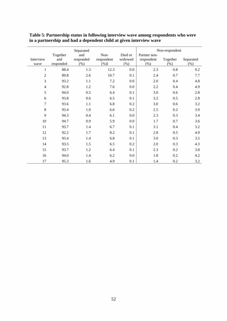
52

Table 5: Partnership status in following interview wave among respondents who were in a partnership and had a dependent child at given interview wave

Interview wave

Together and

responded

Separated and

responded (%)

Non-respondent

(%)l

Died or widowed

(%)

Non-respondent Partner non-respondent

(%) Together

(%) Separated

(%) 1 88.4 1.3 12.3 0.0 2.3 0.8 9.2 2 89.8 2.6 10.7 0.1 2.4 0.7 7.7 3 93.2 1.1 7.2 0.0 2.0 0.4 4.8 4 92.8 1.2 7.6 0.0 2.2 0.4 4.9 5 94.0 0.5 6.4 0.1 3.0 0.6 2.8 6 93.8 0.6 6.5 0.1 3.2 0.5 2.8 7 93.6 1.1 6.8 0.2 3.0 0.6 3.2 8 93.4 1.0 6.6 0.2 2.5 0.2 3.9 9 94.3 0.4 6.1 0.0 2.3 0.3 3.4

10 94.7 0.9 5.9 0.0 1.7 0.7 3.6 11 93.7 1.4 6.7 0.1 3.1 0.4 3.2 12 92.2 1.7 8.2 0.1 2.8 0.5 4.9 13 93.4 1.4 6.8 0.1 3.0 0.3 3.5 14 93.5 1.5 6.5 0.2 2.0 0.3 4.3 15 93.7 1.2 6.4 0.1 2.3 0.2 3.8 16 94.0 1.4 6.2 0.0 1.8 0.2 4.2 17 95.3 1.6 4.9 0.1 1.4 0.2 3.2

53

Table 6. Characteristics measured in interview t of those known to have separated between interview t and t+1, by whether interviewed at t+1

Men Women

Interviewed

at t+1 (%)

Not interviewed

at t+1 (%)

Interviewed at t+1 (%)

Not interviewed

at t+1 (%)

Employed 81.4 74.6 65.8 60.7 Owned outright 6.2 6.0 6.7 9.1 Owned with mortgage 59.2 49.2 53.1 58.2 Social housing 18.0 31.1 23.1 25.5 Other renting 16.6 13.7 17.0 7.3 Cohabiting 48.0 37.0 47.5 33.3 Age 15-19 years 2.6 1.1 7.0 3.5 Age 20-29 years 36.5 34.2 40.0 29.8 Age 30-39 years 30.4 31.5 29.1 26.3 Age 40-49 years 18.6 21.7 17.0 22.8 Age 50-59 years 8.3 8.2 5.1 1.8 Age 60+ years 3.7 3.3 1.9 15.8 No Educational Qualifications 18.9 31.1 18.2 38.8 GCSE/A-level 59.4 52.3 66.5 55.1 College or higher 21.7 16.6 15.3 6.1 BHC Income, 25th percentile 23.0 30.7 25.7 24.4 BHC Income, Median 23.5 29.3 25.4 20.0 BHC Income, 75th percentile 26.5 18.7 24.7 33.3 BHC Income, Max 27.0 21.3 24.3 22.2 Have at least one dependent child 46.5 68.5 55.9 43.9 Interview was in 1991-1999 65.2 72.8 62.7 71.9 Number of observations 652 184 908 57

54

Table 7. Logit estimation of the likelihood of separating by the next wave (GB sample, only OSMs & PSMs, separation does not include death of partner, observed until first separation or last interview)

All Women Men

Odds Ratio Odds Ratio Odds Ratio

Gender (Omitted: Men) Women 1.1

Whether has at least one dependent child (Omitted: No) Has at least one dependent child 0.71** 0.71** 0.72*

Age of youngest child 1.04** 1.05** 1.03* Age group (Omitted: 30-39 years)

Age 15-19 years 3.05** 3.12** 3.13** Age 20-29 years 1.50** 1.64** 1.33* Age 40-49 years 0.58** 0.57** 0.61** Age 50-59 years 0.30** 0.23** 0.38** Age 60+ years 0.10** 0.06** 0.12**

Current marital status (Omitted: Married) Cohabiting 3.57** 3.38** 3.82**

Interview year (Omitted: 1998 – 2003) 1991 – 1997 1.07 1.04 1.08

2004 – 2008 0.91 1.06 0.74* Highest educational qualifications (Omitted: None)

GCSE or A-levels 1.24* 1.35* 1.13 Higher 1.07 1.11 1.02

Current employment status (Omitted: Not employed) Currently employed 0.94 1.05 0.79+

Housing Tenure (Omitted: Owned with mortgage) Owned outright 0.77+ 1.03 0.56*

Renting, Social Housing 1.49** 1.73** 1.24 Renting, Other 1.84** 1.98** 1.71**

Net Current Household BHC income (Omitted: Less than 25th percentile)

25th to 50th percentile 0.84+ 0.84 0.85 50th to 75th percentile 0.74** 0.70** 0.80 75th percentile or higher 0.72** 0.67** 0.78

Constant 0.02** 0.02** 0.03** Number of Observations 64748 32018 32730 + p<0.10, * p<0.05, ** p<.01

Sample is non-TSM GB respondents observed in any wave, but excluding those whose partnership ends through widow(er)hood.

55

Table 8. Logit estimation of the likelihood of separating by the next wave (GB sample, only OSMs & PSMs, separation does not include death of partner, observed until first separation or last interview)

Women with dependent

children in the interview

before separation

Women without dependent

children in the interview before

separation

Men with dependent

children in the interview

before separation

Men without dependent

children in the interview before

separation

Odds Ratio Odds Ratio Odds Ratio Odds Ratio

Age of youngest child 1.04**

1.00 Age group (Omitted: 30-39 years)

Age 15-19 years 3.14** 3.02** 2.12 3.80** Age 20-29 years 1.77** 1.46* 1.30 1.30 Age 40-49 years 0.55** 0.63 0.76 0.47** Age 50-59 years 0.35* 0.21** 0.69 0.31** Age 60+ years

0.06** 0.80 0.11**

Current marital status (Omitted: Married)

Cohabiting 3.05** 3.90** 2.91** 4.63** Interview year (Omitted: 1998 – 2003)

1991 – 1997 1.03 1.09 1.03 1.12 2004 – 2008 0.97 1.21 0.86 0.65*

Highest educational qualifications (Omitted: None)

GCSE or A-levels 1.39* 1.26 1.21 0.98 Higher 1.01 1.14 0.85 1.04

Current employment status (Omitted: Not employed)

Currently employed 1.07 0.99 0.69+ 0.84 Housing Tenure (Omitted: Owned with mortgage)

Owned outright 1.02 0.99 0.81 0.48* Renting, Social Housing 1.78** 1.57+ 1.16 1.39 Renting, Other 1.85** 2.08** 1.50+ 1.75**

Net Current Household BHC income (Omitted: Less than 25th percentile)

25th to 50th percentile 0.93 0.63* 0.87 0.88 50th to 75th percentile 0.74+ 0.63* 0.93 0.75 75th percentile or higher 0.72 0.58* 0.89 0.92

Any biological children

0.97

1.22 Constant 0.01** 0.02** 0.02** 0.02** Number of Observations 14149 17832 13666 18986 + p<0.10, * p<0.05, ** p<.01

56

Table 9. Characteristics of our main sample (all measured in the year before separation; standard deviations for continuous variables in parentheses) Women Men

kids at t-1

No kids at t-1, kids earlier

No kids at t-1 or earlier

kids at t-1

No kids at t-1, kids earlier

No kids at t-1 or earlier

Age group 15-19 year 5% 0% 12% 1% 0% 5% 20-29 years 34% 3% 63% 24% 11% 61% 30-39 years 41% 3% 17% 42% 16% 22% 40-49 years 18% 47% 5% 27% 26% 6% 50-59 years 2% 33% 1% 5% 32% 4% 60+ years 0% 14% 1% 0% 16% 3%

Highest educational qualification

No qualifications 20% 55% 3% 19% 34% 13% A/O level or equivalent 70% 35% 71% 66% 45% 57% Higher degree 10% 10% 25% 15% 20% 30%

Employed 58% 58% 82% 82% 71% 85% Marital Status

Married 65% 76% 24% 72% 64% 24% Cohabiting 35% 24% 76% 28% 36% 76%

Has at least one biological child (ever) 94% 100% 0% 91% 100% 0% House tenure

Owned outright 4% 18% 7% 4% 13% 7% Owned with mortgage 54% 50% 53% 63% 56% 56% Social renting 32% 21% 9% 23% 22% 10% Other types of renting 10% 10% 31% 10% 10% 27%

Real Equivalised Net BHC HH income

< 25th percentile 37% 22% 16% 35% 22% 14% Between 25th percentile and Median 32% 26% 14% 31% 23% 19% Between Median and 75th percentile 20% 26% 30% 25% 29% 26% Above 75th percentile 11% 25% 40% 10% 26% 41%

Real Equivalised Net AHC HH income

< 25th percentile 36% 23% 20% 34% 21% 16% Between 25th percentile and Median 32% 28% 15% 31% 26% 20% Between Median and 75th percentile 20% 26% 26% 24% 30% 23% Above 75th percentile 12% 23% 38% 12% 23% 42%

Year before separation is in 1991-1997 52% 55% 46% 51% 61% 52% 1998-2003 34% 28% 34% 36% 31% 33% 2004-2008 13% 17% 21% 14% 8% 15%

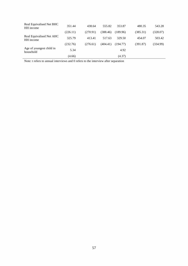
57

Real Equivalised Net BHC HH income 351.44 438.64 555.82 353.87 480.35 543.28

(226.11) (270.91) (388.46) (189.96) (385.31) (328.07) Real Equivalised Net AHC HH income 325.79 413.41 517.63 329.50 454.07 503.42

(232.76) (276.61) (404.41) (194.77) (391.87) (334.99) Age of youngest child in household 5.34 4.92

(4.66) (4.37) Note: t refers to annual interviews and 0 refers to the interview after separation

58

Table 10. Fraction of those who remain single, by number of interviews since separation

Women with dependent children

in the interview before separation

Women without dependent children

in the interview before separation

Men with dependent children

in the interview before separation

Men without dependent children

in the interview before separation

Interviews since first observed as single Survivor SE Survivor SE Survivor SE Survivor SE

1 0.84 0.02 0.80 0.02 0.80 0.03 0.76 0.02 2 0.72 0.02 0.63 0.03 0.66 0.03 0.61 0.03 3 0.63 0.02 0.55 0.03 0.60 0.03 0.51 0.03 4 0.56 0.03 0.50 0.03 0.52 0.03 0.43 0.03 5 0.51 0.03 0.46 0.03 0.49 0.03 0.35 0.03 6 0.47 0.03 0.43 0.03 0.41 0.04 0.34 0.03 7 0.43 0.03 0.40 0.03 0.35 0.04 0.31 0.03 8 0.38 0.03 0.37 0.03 0.35 0.04 0.26 0.03 9 0.36 0.03 0.37 0.03 0.35 0.04 0.25 0.03

10 0.33 0.03 0.36 0.03 0.30 0.04 0.22 0.03 Note: Years refers to annual interviews and 0 refers to the interview after separation

Women with co-resident children in

interview before and after separation

Women with co-resident children in

interview before, but not after, separation

Interviews since first observed as single Survivor SE Survivor SE

1 0.85 0.02 0.73 0.07 2 0.73 0.02 0.68 0.07 3 0.63 0.03 0.66 0.07 4 0.55 0.03 0.63 0.07 5 0.50 0.03 0.63 0.07 6 0.46 0.03 0.53 0.08 7 0.42 0.03 0.50 0.08 8 0.37 0.03 0.46 0.08 9 0.35 0.03 0.42 0.09 10 0.32 0.03 0.38 0.09

Note: Years refers to annual interviews and 0 refers to the interview after separation

59

Table 11. Discrete time hazard model of time to repartnering with a logit hazard function: Estimated Coefficients

Model 1 Model 2

Women Men Women Men

dependent children in the interview before separation

dependent children in the interview before separation

dependent children in the interview before separation

No dependent children in the interview before separation

dependent children in the interview before separation

No dependent children in the interview before separation

dependent children in the interview before separation

No dependent children in the interview before separation

Current employment status (Omitted: Full-time Employed)

Not employed -0.186 -1.002** -0.515+ -0.991** -0.234 -0.852** -0.465+ -0.923** Part time employed -0.242 -0.463+ -0.211 0.022 -0.254 -0.444 -0.186 0.02 Self-employed -0.541 0.282 -0.394 0.056 -0.474 0.256 -0.366 0.092

HH BHC income -0.001 0 0 0 -0.001 0 0 0 Duration Dependence (Omitted: within first interview after separation)

3+ years after separation

-0.483** -1.140** -0.362+ -0.387*

Constant -1.638** -1.582** -1.757** -1.691** -1.472** -1.325** -1.703** -1.604** No. of person-year observations 2232 1419 1156 1209 2232 1419 1156 1209 + p<0.10, * p<0.05, ** p<.01

60

Table 11. Discrete time hazard model of time to repartnering with a logit hazard function: Estimated Coefficients (continued). Model 3

Women with dependent

children in the interview before

separation

Women without dependent

children in the interview before

separation

Men with dependent

children in the interview before

separation

Men without dependent

children in the interview before

separation Current employment status (Omitted: Full-time Employed)

Not employed -0.413* -0.384 -0.024 -0.324 Part time employed -0.378+ -0.218 0.509 0.462 Self-employed -0.33 0.432 -0.18 0.236

HH BHC income 0 0 0 0 Duration Dependence (Omitted: 0-3 years after separation)

3+ years after separation -0.241 -0.783** -0.091 -0.069 Was cohabiting at separation -0.346* 0.444+ -0.005 0.393+

Has at least one dependent child in the household -0.395 0.661 -0.681+ 3.148* Age of youngest dependent child in the household 0.02 0.062 0.02 -0.218 Age group (Omitted: 30-39 years)

15-19 years 0.366 -0.439

0.16 20-29 years 0.675** -0.089 -0.165 -0.239 40-49 years -0.677** -0.819* -0.626* -0.817* 50-59 years -1.249** -1.032+ -1.171** -0.169 60-69 years

-2.268** -1.970* -3.413**

Highest Educational Qualifications (Omitted: Higher degree)

None -0.206 0.835** 0.197 0.212 GCSE/A-levels -0.111 0.281 0.084 0.346

Self-reported health status (Omitted: Fair)

Excellent 0.048 0.814* -0.109 0.394 Good 0.053 1.179+ -0.4 0.606 Poor 0.271 -0.293 0.068 -0.031 Very Poor 0.068 -0.112 0.554+ 0.262

Year of separation (Omitted: 1998 – 2003)

1991 – 1997 -0.174 0.232 -0.029 0.238 2004 – 2008 -0.386 -0.248 0.111 -0.063

Any children prior to separation

0.508

0.519+

Constant -0.964* -1.866** -1.832** -2.429** Number of observations 1894 1261 1028 1033 + p<0.10, * p<0.05, ** p<.01 Note All covariates measured in the interview before the split.

61

Table 12. Employment status by sub-groups Women with

dependent children in the

interview before

separation

Women without dependent

children in the interview

before separation

Men with dependent

children in the interview

before separation

Men without dependent

children in the interview

before separation

All family types

Employed at interview after separation

291 303 246 287 1,127

Not employed at interview after separation

216 97 56 62 431

All 507 400 302 349 1,558

62

Table 13. Estimated fraction remaining out-of-work amongst those not employed at interview after separation

Women with dependent

children in the interview before

separation

Women without dependent

children in the interview before

separation

Men with dependent

children in the interview before

separation

Men without dependent

children in the interview before

separation Interviews since first

observed as single N

Survivor SE N

Survivor SE N

Survivor SE N Survivor SE

1 200 0.82 0.03 98 0.76 0.04 51 0.73 0.06 57 0.74 0.06 2 148 0.71 0.03 69 0.62 0.05 32 0.59 0.07 35 0.63 0.07 3 113 0.62 0.04 51 0.56 0.05 23 0.56 0.07 26 0.58 0.07 4 91 0.55 0.04 40 0.49 0.05 17 0.43 0.08 23 0.53 0.07 5 75 0.43 0.04 30 0.48 0.05 11 0.35 0.08 19 0.53 0.07 6 54 0.33 0.04 28 0.48 0.05

17 0.53 0.07

7 35 0.29 0.04 23 0.46 0.06

12 0.53 0.07 8 28 0.26 0.04 19 0.46 0.06

8 0.53 0.07

9 23 0.22 0.04 17 0.43 0.06 10 16 0.19 0.04 14 0.43 0.06 Note: Years refers to annual interviews and 0 refers to the interview after separation

Women with co-resident children in interview before

and after separation

Women with co-resident children in interview before,

but not after, separation Interviews since first observed as single N Survivor SE N Survivor SE

1 170 0.84 0.03 30 0.73 0.08 2 128 0.73 0.03 20 0.59 0.09 3 99 0.63 0.04 14 0.54 0.09 4 80 0.58 0.04 11 0.35 0.10 5 68 0.45 0.04 7 0.30 0.10 6 48 0.35 0.04 6 0.25 0.09 7 31 0.30 0.04 4 0.19 0.09 8 25 0.28 0.04 3 0.12 0.08 9 21 0.24 0.04

10 14 0.20 0.04 Note: Years refers to annual interviews and 0 refers to the interview after

separation

63

Table 14. Partnership and employment status among those who become lone mothers and who are in work at the interview after separation

Interviews since first observed as single

partnered, employed

partnered, not

employed

not partnered, employed

not partnered,

not employed

Partnered Employed

% Partnered

among employed

% Partnered

among not

employed 0 8.9 0.0 91.1 0.0 8.9 100 9% 1 21.4 2.6 70.1 5.9 24 91.5 23% 31% 2 25.4 6.0 62.1 6.5 31.4 87.5 29% 48% 3 30.8 6.4 54.7 8.1 37.2 85.5 36% 44% 4 31.5 8.8 54.6 5.1 40.3 86.1 37% 63% 5 34.0 8.4 52.9 4.7 42.4 86.9 39% 64% 6 38.3 6.6 50.9 4.2 44.9 89.2 43% 61% 7 37.9 7.6 48.3 6.2 45.5 86.2 44% 55% 8 37.7 10.0 46.9 5.4 47.7 84.6 45% 65% 9 38.9 9.7 45.1 6.2 48.6 84 46% 61%

10 47.0 9.0 36.0 8.0 56 83 57% 53% Note: Years refers to annual interviews, and year 0 is the interview after separation. Table 15. Partnership and employment status among those who become lone mothers and who are not in work at the interview after separation Interviews since first observed as single

partnered, employed

partnered, not

employed

not partnered, employed

not partnered,

not employed

Partnered Employed

% Partnered

among employed

% Partnered among not employed

0 0.0 9.3 0.0 90.7 9.3 0 9% 1 5.2 16.7 17.7 60.4 21.9 22.9 23% 22% 2 8.6 21.6 17.8 51.9 30.2 26.4 33% 29% 3 10.3 26.1 25.5 38.2 36.4 35.8 29% 41% 4 15.3 23.6 28.0 33.1 38.9 43.3 35% 42% 5 18.8 20.1 30.6 30.6 38.9 49.4 38% 40% 6 23.4 19.5 28.9 28.1 42.9 52.3 45% 41% 7 25.0 19.8 34.5 20.7 44.8 59.5 42% 49% 8 31.1 19.8 27.4 21.7 50.9 58.5 53% 48% 9 30.6 26.5 27.6 15.3 57.1 58.2 53% 63%

10 32.6 24.4 27.9 15.1 57 60.5 54% 62% Note: Years refers to annual interviews, and year 0 is the interview after separation.

64

Table 16. Mean percentage changes since separation in net equivalised household income, un-equivalised household income and equivalence scale

Years since

separation Women with dependent children

in the year before separation

Women without dependent children in the year before separation, but

had children earlier Women without dependent

children, ever

Equiv

inc Unequiv

inc Equiv scale Equiv inc

Unequiv inc

Equiv scale

Equiv inc

Unequiv inc

Equiv scale

-2 0.00 0.00 0.00 0.00 0.00 0.00 0.00 0.00 0.00 -1 9.98 13.74 3.20 9.32 8.48 -0.82 23.26 31.08 1.66 0 -3.27 -15.99 -16.44 -8.22 -36.79 -31.61 12.10 12.86 -10.76 1 7.24 -5.77 -14.45 -6.13 -31.81 -29.51 14.52 13.24 -11.78 2 16.71 3.83 -12.64 19.24 -6.56 -26.84 32.20 37.99 -5.95 3 17.05 7.86 -10.39 29.10 -1.30 -27.32 41.71 55.48 -0.54 4 23.66 14.39 -9.01 14.51 -14.01 -28.17 59.54 61.42 -4.15 5 25.99 18.16 -7.82 26.24 -1.72 -26.10 59.21 55.12 -3.91 6 36.80 32.66 -5.55 41.00 10.58 -26.20 45.23 38.59 -3.28 7 45.82 43.00 -4.05 39.39 9.93 -24.78 50.56 48.33 -1.70 8 53.07 53.79 -1.91 67.83 35.77 -23.06 53.34 64.57 2.64 9 56.63 51.60 -2.36 58.72 21.35 -23.36 43.33 55.96 6.29

10 55.07 52.82 -2.46 80.58 34.55 -23.99 23.79 31.95 7.00 Note: Years refers to annual interviews, and year 0 is the interview after separation

Years since

separation Men with dependent children in

the year before separation

Men without dependent children in the year before separation, but had

children earlier Men without dependent

children, ever

Equiv inc

Unequiv inc

Equiv scale Equiv inc

Unequiv inc

Equiv scale

Equiv inc

Unequiv inc

Equiv scale

-2 0.00 0.00 0.00 0.00 0.00 0.00 0.00 0.00 0.00 -1 6.69 7.89 1.10 7.31 7.53 -0.56 31.45 32.80 1.32 0 41.68 -7.81 -33.74 17.15 -14.03 -25.40 32.25 15.98 -15.24 1 45.01 -1.06 -29.72 18.04 -8.55 -17.66 21.38 8.69 -12.15 2 62.93 13.94 -27.47 33.35 0.79 -20.99 28.40 15.78 -10.02 3 48.02 -0.89 -28.61 35.84 3.05 -19.36 35.71 25.41 -7.87 4 63.51 21.98 -26.38 6.54 -16.66 -21.10 32.26 20.18 -5.63 5 58.57 11.06 -26.64 29.15 0.33 -17.64 28.78 21.00 -2.83 6 65.28 20.86 -24.23 52.49 16.69 -18.85 34.33 29.36 -0.76 7 56.98 20.75 -22.30 55.76 17.68 -18.97 55.23 52.81 1.95 8 71.31 32.38 -22.42 48.32 15.68 -18.15 48.04 39.22 -2.52 9 68.15 30.07 -22.39 57.87 29.84 -12.61 49.52 45.24 -0.19

10 80.56 49.18 -16.79 117.61 69.84 -8.23 29.49 24.23 -1.27 Note: Years refers to annual interviews, and year 0 is the interview after separation

65

Table 17: Mean Change in BHC Income Components, among those with BHC income ABOVE median BHC income measured 2 interviews before separation Women with dependent children at t=-1

Total Net Labour

Net Labour Investment Benefits Pensions Transfers Local Taxes Own Partner Other

-2 0.00 0.00 0.00 0.00 0.00 0.00 0.00 0.00 0.00 0.00 -1 -20.93 -18.07 -1.13 6.34 -23.28 -7.24 7.81 -2.59 -0.16 0.40 0 -361.91 -412.52 20.10 -438.70 6.08 -21.94 36.59 -3.75 36.15 -3.52 1 -332.35 -387.19 18.75 -389.77 -16.17 -17.49 33.35 -4.81 40.56 -3.23 2 -181.65 -243.56 136.03 -373.32 -6.27 -15.44 40.28 -1.41 36.62 -1.93 3 -261.47 -320.83 41.09 -343.42 -18.50 -16.48 34.96 0.38 39.86 -0.79 4 -284.20 -334.17 38.64 -357.94 -14.87 -15.39 32.31 -0.81 34.83 0.99 5 -264.14 -309.61 55.10 -347.64 -17.06 -20.16 25.38 1.26 40.57 2.02 6 -253.08 -299.52 55.25 -341.09 -13.68 -22.50 43.09 -0.26 29.75 3.64 7 -229.04 -285.61 60.38 -338.07 -7.92 0.12 33.60 -2.51 30.15 4.78 8 -197.54 -252.60 50.65 -289.28 -13.97 1.25 31.75 3.82 23.47 5.23 9 -143.55 -181.09 59.85 -261.30 20.36 8.65 17.42 -1.51 18.31 5.81

10 -116.43 -130.66 66.07 -221.42 24.69 -0.43 -8.42 2.70 28.11 7.74 Men with dependent children at t=-1

Total Net

Labour Net Labour Investment Benefits Pensions Transfers Local

Taxes Own Partner Other -2 0.00 0.00 0.00 0.00 0.00 0.00 0.00 0.00 0.00 0.00 -1 -42.22 -32.89 -13.00 -1.16 -18.73 -4.65 -2.00 0.32 -2.37 0.27 0 -234.38 -176.45 -41.49 -144.81 9.85 -16.36 -46.71 5.36 -3.69 -3.44 1 -149.12 -127.89 -22.93 -121.52 17.41 -7.04 -23.18 8.76 -2.25 -2.68 2 -127.11 -122.76 -26.47 -103.82 7.53 -1.31 -14.37 11.53 -1.44 -1.33 3 -143.94 -150.04 -30.05 -103.57 -16.42 -3.55 -4.65 14.25 -0.16 -1.10 4 -115.55 -138.71 -18.81 -88.82 -31.08 1.55 2.22 19.88 1.20 1.20 5 -68.98 -94.53 4.76 -70.10 -29.19 0.00 6.77 22.59 -1.55 2.33 6 -20.10 -50.91 9.11 -28.33 -31.69 9.83 3.75 21.08 0.45 3.90 7 -16.85 -41.02 -16.78 -23.46 -0.78 12.41 -2.53 16.30 2.26 4.26 8 27.55 -16.57 -6.99 -27.18 17.60 18.26 10.34 18.10 3.10 5.71 9 18.90 -11.54 -47.26 25.05 10.66 10.23 6.41 17.49 1.35 5.82

10 220.20 180.15 117.68 -0.24 62.72 19.43 3.83 31.13 -5.91 8.43 Note: Years refers to annual interviews, and year 0 is the interview after separation

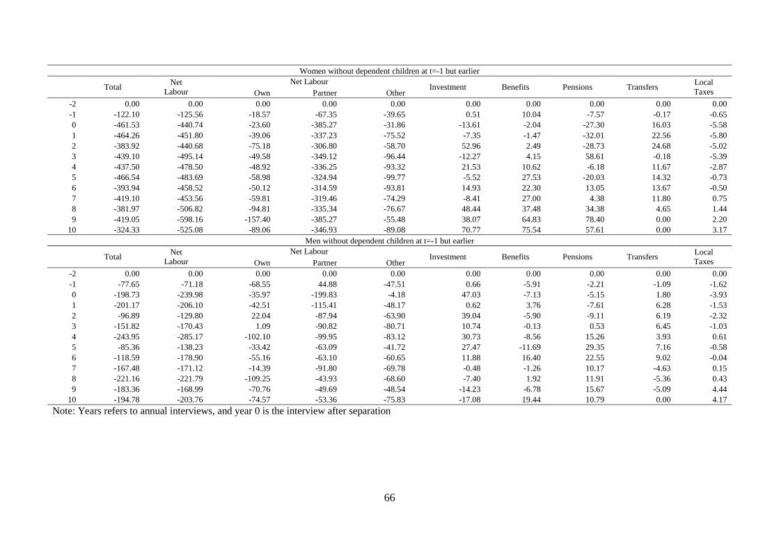
66

Women without dependent children at t=-1 but earlier

Total Net

Labour Net Labour Investment Benefits Pensions Transfers Local

Taxes Own Partner Other -2 0.00 0.00 0.00 0.00 0.00 0.00 0.00 0.00 0.00 0.00 -1 -122.10 -125.56 -18.57 -67.35 -39.65 0.51 10.04 -7.57 -0.17 -0.65 0 -461.53 -440.74 -23.60 -385.27 -31.86 -13.61 -2.04 -27.30 16.03 -5.58 1 -464.26 -451.80 -39.06 -337.23 -75.52 -7.35 -1.47 -32.01 22.56 -5.80 2 -383.92 -440.68 -75.18 -306.80 -58.70 52.96 2.49 -28.73 24.68 -5.02 3 -439.10 -495.14 -49.58 -349.12 -96.44 -12.27 4.15 58.61 -0.18 -5.39 4 -437.50 -478.50 -48.92 -336.25 -93.32 21.53 10.62 -6.18 11.67 -2.87 5 -466.54 -483.69 -58.98 -324.94 -99.77 -5.52 27.53 -20.03 14.32 -0.73 6 -393.94 -458.52 -50.12 -314.59 -93.81 14.93 22.30 13.05 13.67 -0.50 7 -419.10 -453.56 -59.81 -319.46 -74.29 -8.41 27.00 4.38 11.80 0.75 8 -381.97 -506.82 -94.81 -335.34 -76.67 48.44 37.48 34.38 4.65 1.44 9 -419.05 -598.16 -157.40 -385.27 -55.48 38.07 64.83 78.40 0.00 2.20

10 -324.33 -525.08 -89.06 -346.93 -89.08 70.77 75.54 57.61 0.00 3.17 Men without dependent children at t=-1 but earlier

Total Net

Labour Net Labour Investment Benefits Pensions Transfers Local

Taxes Own Partner Other -2 0.00 0.00 0.00 0.00 0.00 0.00 0.00 0.00 0.00 0.00 -1 -77.65 -71.18 -68.55 44.88 -47.51 0.66 -5.91 -2.21 -1.09 -1.62 0 -198.73 -239.98 -35.97 -199.83 -4.18 47.03 -7.13 -5.15 1.80 -3.93 1 -201.17 -206.10 -42.51 -115.41 -48.17 0.62 3.76 -7.61 6.28 -1.53 2 -96.89 -129.80 22.04 -87.94 -63.90 39.04 -5.90 -9.11 6.19 -2.32 3 -151.82 -170.43 1.09 -90.82 -80.71 10.74 -0.13 0.53 6.45 -1.03 4 -243.95 -285.17 -102.10 -99.95 -83.12 30.73 -8.56 15.26 3.93 0.61 5 -85.36 -138.23 -33.42 -63.09 -41.72 27.47 -11.69 29.35 7.16 -0.58 6 -118.59 -178.90 -55.16 -63.10 -60.65 11.88 16.40 22.55 9.02 -0.04 7 -167.48 -171.12 -14.39 -91.80 -69.78 -0.48 -1.26 10.17 -4.63 0.15 8 -221.16 -221.79 -109.25 -43.93 -68.60 -7.40 1.92 11.91 -5.36 0.43 9 -183.36 -168.99 -70.76 -49.69 -48.54 -14.23 -6.78 15.67 -5.09 4.44

10 -194.78 -203.76 -74.57 -53.36 -75.83 -17.08 19.44 10.79 0.00 4.17 Note: Years refers to annual interviews, and year 0 is the interview after separation

67

Women without dependent children at t=-1 or earlier

Total Net

Labour Net Labour

Investment Benefits Pensions Transfers Local Taxes Own Partner Other

-2 0.00 0.00 0.00 0.00 0.00 0.00 0.00 0.00 0.00 0.00 -1 -14.18 13.60 30.02 66.39 -82.81 -8.40 0.71 -2.71 -18.06 -0.87 0 -216.17 -181.50 24.38 -221.02 15.14 -15.39 6.03 -6.61 -21.52 -2.97 1 -204.63 -186.23 31.73 -194.36 -23.61 -9.54 16.08 -3.71 -23.36 -2.44 2 -165.09 -145.75 27.59 -146.02 -27.32 -8.58 18.72 -0.86 -29.21 -0.70 3 -94.22 -88.44 45.36 -124.73 -9.08 -4.62 21.47 3.71 -25.61 0.40 4 -91.58 -77.85 56.39 -92.37 -41.87 -2.58 20.74 3.55 -33.50 1.73 5 -115.63 -87.57 50.32 -62.38 -75.51 -10.12 19.42 -0.04 -35.11 2.53 6 -142.95 -118.44 60.17 -91.58 -87.04 -9.55 23.22 1.62 -37.64 2.85 7 -100.81 -90.92 71.26 -63.57 -98.62 -3.08 38.61 -3.00 -39.05 3.61 8 -40.12 -36.52 69.15 -14.69 -90.97 7.25 37.13 2.90 -46.15 4.73 9 2.33 21.79 45.28 63.40 -86.89 -3.72 36.01 4.13 -50.35 5.52

10 -22.89 -37.60 20.80 -2.80 -55.61 16.30 44.36 15.67 -56.05 5.57 Men without dependent children at t=-1 or earlier

Total Net

Labour Net Labour

Investment Benefits Pensions Transfers Local Taxes Own Partner Other

-2 0.00 0.00 0.00 0.00 0.00 0.00 0.00 0.00 0.00 0.00 -1 -52.11 -41.04 40.95 35.88 -117.87 -4.75 3.93 0.97 -11.45 -0.09 0 -171.16 -148.09 33.55 -170.58 -11.06 -4.41 -4.57 2.98 -18.75 -1.88 1 -114.24 -90.48 54.53 -131.47 -13.54 -9.39 1.81 4.57 -21.69 -1.17 2 -67.50 -58.09 88.54 -83.97 -62.66 0.59 5.86 3.41 -19.19 0.01 3 -41.22 -35.97 84.16 -55.94 -64.20 -6.70 11.75 5.11 -15.07 0.39 4 11.45 10.67 99.87 -26.53 -62.68 3.68 12.17 2.97 -15.78 2.38 5 -25.72 -28.53 58.75 -7.84 -79.44 15.71 5.84 2.93 -18.59 4.24 6 19.70 13.62 101.12 2.77 -90.27 13.70 13.79 1.47 -19.55 3.55 7 52.50 79.71 146.27 31.15 -97.71 -7.28 9.80 1.49 -26.95 5.46 8 -27.77 -19.67 87.83 6.33 -113.83 6.39 18.41 -1.25 -25.79 6.27 9 -1.31 23.89 129.69 -6.80 -99.00 -5.26 17.53 -1.46 -30.33 6.72

10 -107.59 -95.87 67.88 -44.60 -119.15 1.33 27.11 -0.83 -32.69 7.17 Note: Years refers to annual interviews, and year 0 is the interview after separation

68

Table 18: Mean Change in BHC Income Components, among those with BHC income BELOW median BHC income measured 2 interviews before separation Women with dependent children at t=-1

Total Net Labour

Net Labour Investment Benefits Pensions Transfers Local Taxes Own Partners Other

-2 0.00 0.00 0.00 0.00 0.00 0.00 0.00 0.00 0.00 0.00 -1 38.93 19.16 5.67 15.36 -1.87 3.62 13.81 0.28 1.82 -0.35 0 -47.42 -118.08 11.94 -148.34 18.32 1.07 49.65 0.06 16.47 -3.37 1 -6.42 -74.54 29.15 -122.05 18.35 -0.19 48.28 0.68 16.58 -2.83 2 13.55 -59.39 29.13 -108.94 22.37 3.45 52.66 1.67 13.39 -1.76 3 47.13 -27.01 38.69 -86.19 20.50 1.06 55.20 1.50 15.59 -1.05 4 72.55 5.88 47.98 -66.21 24.11 4.92 41.93 2.46 17.54 -0.06 5 92.48 33.72 50.87 -60.91 43.76 4.15 42.16 1.03 12.09 0.52 6 131.20 59.40 60.44 -43.64 42.60 3.14 58.51 -0.08 11.74 1.51 7 167.55 92.16 62.70 -21.75 51.20 -1.15 71.58 0.01 7.00 1.89 8 222.76 111.67 98.45 -45.48 58.70 0.97 98.51 0.34 14.38 3.21 9 207.56 138.81 98.88 -16.90 56.84 0.17 56.07 4.92 11.98 4.39

10 175.25 137.96 95.84 -25.99 68.10 -2.65 39.68 0.00 5.44 5.18 Men with dependent children at t=-1

Total Net Labour

Net Labour Investment Benefits Pensions Transfers Local Taxes Own Partners Other

-2 0.00 0.00 0.00 0.00 0.00 0.00 0.00 0.00 0.00 0.00 -1 29.98 11.40 1.32 5.15 4.94 3.56 13.36 0.32 1.47 0.14 0 -9.92 -11.69 0.82 -63.35 50.84 2.25 -12.88 9.10 0.48 -2.45 1 12.56 16.35 14.89 -39.40 40.86 1.46 -18.60 8.15 2.64 -1.70 2 59.33 60.34 40.00 -14.20 34.54 8.08 -16.84 5.44 0.53 -1.34 3 17.47 21.83 22.88 -19.38 18.32 -2.44 -7.32 4.55 -0.61 -0.80 4 124.02 107.72 108.70 -22.10 21.13 1.79 -0.90 4.23 10.85 0.00 5 36.83 27.50 45.97 -31.97 13.50 -1.62 4.51 5.57 1.16 0.69 6 88.70 50.08 40.96 -12.03 21.15 27.61 1.10 10.34 0.64 1.94 7 105.62 73.30 49.85 8.91 14.53 9.13 18.37 6.77 0.88 3.22 8 148.42 131.54 55.85 34.77 40.92 8.48 7.40 4.80 0.02 4.03 9 141.44 139.23 52.55 58.48 28.21 16.50 -14.07 6.66 -1.52 5.91

10 170.92 163.29 78.01 56.14 29.14 -1.80 9.41 6.31 -0.87 5.43 Note: Years refers to annual interviews, and year 0 is the interview after separation

69

Women without dependent children at t=-1 but earlier

Total Net Labour

Net Labour Investment Benefits Pensions Transfers Local Taxes Own Partners Other

-2 0.00 0.00 0.00 0.00 0.00 0.00 0.00 0.00 0.00 0.00 -1 36.07 10.59 5.95 9.10 -4.46 1.28 18.82 0.55 3.86 -0.98 0 -126.43 -48.09 19.11 -30.59 -36.61 -5.44 -56.77 -21.43 0.00 -4.95 1 -127.07 -62.05 3.03 -23.26 -41.83 -6.73 -43.98 -18.70 0.00 -4.07 2 -61.16 -57.68 16.41 -39.54 -34.55 1.98 -4.47 -8.37 4.18 -2.81 3 -25.89 -22.57 17.25 -12.17 -27.65 -2.87 -0.08 -5.23 2.41 -1.54 4 -48.38 -56.24 -5.39 -7.92 -42.93 7.02 9.91 -11.03 0.00 -1.50 5 6.08 8.40 11.47 8.55 -11.62 -3.24 13.49 -16.44 2.15 -1.22 6 35.48 15.13 -6.55 23.59 -1.91 -4.62 36.50 -13.06 2.32 0.92 7 4.90 14.60 4.76 14.23 -4.39 -6.33 9.81 -14.64 2.79 1.32 8 68.88 39.08 4.01 35.36 -0.28 -3.88 41.27 -10.83 3.04 -0.20 9 77.98 25.14 3.71 16.73 4.70 -3.87 49.57 4.61 4.02 1.49

10 53.03 3.06 12.09 16.02 -25.05 -7.95 52.48 -0.09 1.96 -2.88 Men without dependent children at t=-1 but earlier

Total Net Labour

Net Labour Investment Benefits Pensions Transfers Local Taxes Own Partners Other

-2 0.00 0.00 0.00 0.00 0.00 0.00 0.00 0.00 0.00 0.00 -1 13.21 -12.77 2.58 16.22 -31.57 11.72 10.05 3.79 -0.99 -1.41 0 -44.32 -40.96 40.93 -62.77 -19.11 19.77 -18.32 3.74 -10.83 -1.78 1 -51.12 -70.17 4.21 -42.92 -31.47 7.35 15.43 4.28 -9.14 -1.12 2 -78.50 -75.26 1.30 -45.27 -31.29 3.13 0.12 3.71 -12.69 -2.48 3 -45.29 -39.58 22.81 -51.43 -10.97 0.43 2.45 2.26 -13.84 -2.31 4 9.65 4.01 39.41 8.05 -43.46 13.53 -15.32 18.93 -15.62 -3.38 5 13.99 -13.36 63.34 -30.25 -46.44 21.81 11.09 -3.48 -6.73 -3.73 6 18.46 -8.11 62.87 -27.85 -43.13 18.35 8.01 0.16 -2.94 -2.99 7 16.39 8.20 52.74 -1.42 -43.13 6.83 14.48 -0.51 -14.83 -2.22 8 11.76 -8.56 32.54 7.92 -49.03 4.62 31.28 3.72 -23.07 -3.78 9 0.44 -49.57 -11.66 22.01 -59.92 -3.52 73.73 4.18 -28.20 -2.06

10 93.76 22.57 77.55 10.55 -65.54 -3.63 74.02 26.74 -29.21 -3.27 Note: Years refers to annual interviews, and year 0 is the interview after separation

70

Women without dependent children at t=-1 or earlier

Total Net Labour

Net Labour Investment Benefits Pensions Transfers Local Taxes Own Partners Other

-2 0.00 0.00 0.00 0.00 0.00 0.00 0.00 0.00 0.00 0.00 -1 103.70 131.12 33.23 140.66 -42.78 0.10 -19.50 -2.35 -3.98 1.68 0 129.03 148.88 46.71 -9.80 111.97 3.16 -5.24 -0.52 -15.57 2.09 1 130.03 152.66 75.03 8.03 69.60 5.44 -22.79 0.72 -5.61 1.01 2 204.67 227.50 86.50 71.01 69.99 9.99 -9.22 0.41 -20.40 4.36 3 316.19 361.98 125.79 134.42 101.78 6.25 -18.88 -3.79 -24.04 6.40 4 389.18 433.96 239.98 149.49 44.49 6.94 -10.23 6.11 -40.70 6.89 5 310.98 333.40 140.51 173.99 18.90 18.86 7.86 -4.01 -36.64 8.49 6 307.44 346.50 126.49 223.64 0.15 -2.81 1.18 -4.87 -24.72 7.84 7 347.98 390.72 163.61 236.97 -9.85 9.09 -2.68 -5.24 -35.66 8.25 8 355.21 364.48 137.88 236.60 -10.00 -1.64 19.97 -6.20 -12.91 8.49 9 273.56 277.57 120.12 225.59 -54.93 1.12 25.05 -6.79 -14.41 8.98

10 216.95 198.63 79.77 168.37 -49.51 6.77 34.55 0.00 -14.90 8.09 Men without dependent children at t=-1 or earlier

Total Net Labour

Net Labour Investment Benefits Pensions Transfers Local Taxes Own Partners Other

-2 0.00 0.00 0.00 0.00 0.00 0.00 0.00 0.00 0.00 0.00 -1 151.12 121.46 61.35 79.45 -19.34 -1.40 -21.51 -0.91 53.05 -0.44 0 29.86 52.13 71.28 -50.79 31.64 -3.85 -12.68 -1.06 -8.17 -3.19 1 85.17 106.68 99.37 -35.62 42.94 0.37 -20.06 4.08 -8.62 -2.20 2 104.88 123.10 133.94 -14.44 3.60 2.32 -30.88 9.78 -2.21 -2.77 3 165.67 150.53 93.70 10.38 46.45 3.80 -0.60 9.35 1.59 -1.00 4 67.93 73.51 89.70 -6.37 -9.82 -1.74 -6.73 -1.61 3.66 -0.83 5 175.39 126.24 106.46 15.60 4.18 9.73 38.05 -3.58 3.69 -1.26 6 182.62 187.65 123.40 71.95 -7.70 -4.79 -1.69 2.63 -0.68 0.50 7 281.46 276.77 154.52 134.54 -12.29 -2.46 -0.87 7.53 -0.79 -1.28 8 286.16 306.61 158.64 186.14 -38.17 -7.35 -19.06 1.36 -1.15 -4.46 9 313.04 334.33 178.67 159.04 -3.39 -7.46 -14.59 -0.59 -1.15 -2.50

10 228.53 217.29 126.51 118.67 -27.89 -4.85 17.24 -0.79 -1.15 -0.79 Note: Years refers to annual interviews, and year 0 is the interview after separation

71

Table 19: Mean Change in AHC Income Components, among those with AHC income ABOVE median AHC income measured 2 interviews before separation Women with dependent children at t=-1

Total Net Labour

Net Labour Investment Benefits Pensions Transfers

Local Taxes

Housing Cost Own Partner Other

-2 0.00 0.00 0.00 0.00 0.00 0.00 0.00 0.00 0.00 0.00 0.00 -1 -14.55 -12.39 0.07 12.49 -24.95 -6.61 10.85 -2.30 -0.14 0.16 3.43 0 -353.73 -399.58 19.66 -418.42 -0.82 -19.15 41.67 -3.23 34.19 -3.67 15.78 1 -316.80 -364.72 21.76 -367.35 -19.14 -14.44 39.06 -4.20 38.75 -3.49 16.95 2 -175.04 -239.11 119.88 -350.77 -6.70 -6.09 44.76 -1.14 36.68 -1.91 14.11 3 -234.57 -291.39 41.45 -320.88 -11.96 -10.02 39.46 0.39 37.22 -0.51 12.09 4 -219.32 -284.13 42.56 -318.57 -8.13 -4.22 39.29 0.88 37.58 1.11 12.14 5 -221.71 -265.04 53.71 -319.10 0.35 -13.15 31.42 1.11 38.64 2.57 13.23 6 -210.88 -259.93 61.77 -319.86 -1.84 -15.31 48.62 -0.22 29.17 3.64 9.21 7 -217.15 -259.42 63.66 -322.96 -0.12 0.10 37.93 -2.25 29.00 4.59 13.63 8 -120.67 -212.91 66.18 -277.98 -1.12 3.60 77.35 4.02 23.06 5.62 10.15 9 -155.45 -163.92 71.15 -260.39 25.32 8.35 21.12 -1.97 18.98 6.14 13.70

10 -112.60 -110.42 84.61 -229.06 34.02 -0.09 -2.93 1.82 26.18 8.09 8.13 Men with dependent children at t=-1

Total Net Labour

Net Labour Investment Benefits Pensions Transfers

Local Taxes

Housing Cost Own Partner Other

-2 0.00 0.00 0.00 0.00 0.00 0.00 0.00 0.00 0.00 0.00 0.00 -1 -32.96 -26.95 -12.68 2.38 -16.64 -3.82 2.49 0.29 -2.03 0.03 2.60 0 -206.88 -149.12 -29.14 -139.24 19.26 -14.54 -42.23 4.60 -2.69 -3.78 8.34 1 -152.18 -108.44 -11.79 -112.08 16.34 -10.01 -24.89 7.44 -1.05 -2.50 10.52 2 -124.15 -106.68 -20.34 -94.48 8.13 -1.21 -11.53 11.72 -0.28 -1.31 13.17 3 -144.54 -136.87 -31.75 -94.46 -10.66 -2.76 -7.96 14.11 0.51 -1.29 14.38 4 -133.09 -132.03 -26.53 -82.48 -23.02 1.74 -2.25 18.68 2.03 0.65 15.08 5 -117.72 -98.17 -11.16 -71.18 -15.83 0.69 3.32 20.63 -1.02 1.75 21.17 6 -60.06 -71.28 -7.84 -38.28 -25.16 8.26 2.18 20.29 -0.01 3.39 16.69 7 -14.20 -42.48 -24.44 -22.36 4.31 14.86 8.12 17.68 2.09 4.07 14.56 8 39.83 -6.79 -1.34 -23.62 18.17 20.00 12.11 20.23 2.85 4.88 11.89 9 15.48 -3.56 -35.06 26.33 5.17 14.08 4.40 21.18 1.41 5.25 26.22

10 199.73 186.35 117.12 12.68 56.55 16.76 -0.21 34.38 -5.04 7.66 24.85 Note: Years refers to annual interviews, and year 0 is the interview after separation

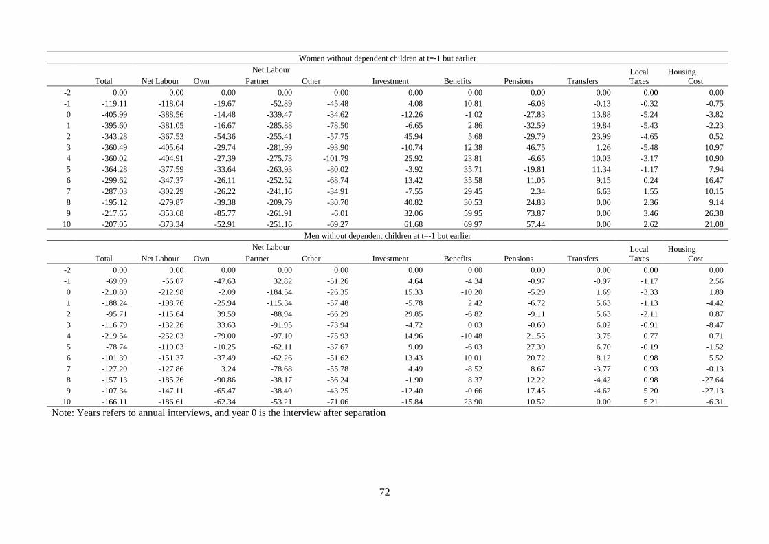
72

Women without dependent children at t=-1 but earlier

Total Net Labour

Net Labour Investment Benefits Pensions Transfers

Local Taxes

Housing Cost Own Partner Other

-2 0.00 0.00 0.00 0.00 0.00 0.00 0.00 0.00 0.00 0.00 0.00 -1 -119.11 -118.04 -19.67 -52.89 -45.48 4.08 10.81 -6.08 -0.13 -0.32 -0.75 0 -405.99 -388.56 -14.48 -339.47 -34.62 -12.26 -1.02 -27.83 13.88 -5.24 -3.82 1 -395.60 -381.05 -16.67 -285.88 -78.50 -6.65 2.86 -32.59 19.84 -5.43 -2.23 2 -343.28 -367.53 -54.36 -255.41 -57.75 45.94 5.68 -29.79 23.99 -4.65 0.52 3 -360.49 -405.64 -29.74 -281.99 -93.90 -10.74 12.38 46.75 1.26 -5.48 10.97 4 -360.02 -404.91 -27.39 -275.73 -101.79 25.92 23.81 -6.65 10.03 -3.17 10.90 5 -364.28 -377.59 -33.64 -263.93 -80.02 -3.92 35.71 -19.81 11.34 -1.17 7.94 6 -299.62 -347.37 -26.11 -252.52 -68.74 13.42 35.58 11.05 9.15 0.24 16.47 7 -287.03 -302.29 -26.22 -241.16 -34.91 -7.55 29.45 2.34 6.63 1.55 10.15 8 -195.12 -279.87 -39.38 -209.79 -30.70 40.82 30.53 24.83 0.00 2.36 9.14 9 -217.65 -353.68 -85.77 -261.91 -6.01 32.06 59.95 73.87 0.00 3.46 26.38

10 -207.05 -373.34 -52.91 -251.16 -69.27 61.68 69.97 57.44 0.00 2.62 21.08 Men without dependent children at t=-1 but earlier

Total Net Labour

Net Labour Investment Benefits Pensions Transfers

Local Taxes

Housing Cost Own Partner Other

-2 0.00 0.00 0.00 0.00 0.00 0.00 0.00 0.00 0.00 0.00 0.00 -1 -69.09 -66.07 -47.63 32.82 -51.26 4.64 -4.34 -0.97 -0.97 -1.17 2.56 0 -210.80 -212.98 -2.09 -184.54 -26.35 15.33 -10.20 -5.29 1.69 -3.33 1.89 1 -188.24 -198.76 -25.94 -115.34 -57.48 -5.78 2.42 -6.72 5.63 -1.13 -4.42 2 -95.71 -115.64 39.59 -88.94 -66.29 29.85 -6.82 -9.11 5.63 -2.11 0.87 3 -116.79 -132.26 33.63 -91.95 -73.94 -4.72 0.03 -0.60 6.02 -0.91 -8.47 4 -219.54 -252.03 -79.00 -97.10 -75.93 14.96 -10.48 21.55 3.75 0.77 0.71 5 -78.74 -110.03 -10.25 -62.11 -37.67 9.09 -6.03 27.39 6.70 -0.19 -1.52 6 -101.39 -151.37 -37.49 -62.26 -51.62 13.43 10.01 20.72 8.12 0.98 5.52 7 -127.20 -127.86 3.24 -78.68 -55.78 4.49 -8.52 8.67 -3.77 0.93 -0.13 8 -157.13 -185.26 -90.86 -38.17 -56.24 -1.90 8.37 12.22 -4.42 0.98 -27.64 9 -107.34 -147.11 -65.47 -38.40 -43.25 -12.40 -0.66 17.45 -4.62 5.20 -27.13

10 -166.11 -186.61 -62.34 -53.21 -71.06 -15.84 23.90 10.52 0.00 5.21 -6.31 Note: Years refers to annual interviews, and year 0 is the interview after separation

73

Women without dependent children at t=-1 or earlier

Total Net Labour

Net Labour Investment Benefits Pensions Transfers

Local Taxes

Housing Cost Own Partner Other

-2 0.00 0.00 0.00 0.00 0.00 0.00 0.00 0.00 0.00 0.00 0.00 -1 -13.23 21.11 26.10 81.76 -86.74 -7.67 -0.52 -3.72 -18.89 -0.66 2.29 0 -219.92 -192.58 18.94 -221.49 9.97 -11.12 9.07 -0.68 -21.58 -2.71 6.11 1 -209.94 -193.69 32.83 -195.57 -30.95 -5.53 15.87 1.17 -24.54 -2.50 5.94 2 -157.08 -136.72 32.79 -144.85 -24.66 -6.08 22.05 1.01 -30.93 -0.37 7.53 3 -104.23 -89.18 50.85 -120.88 -19.14 -3.85 20.90 4.33 -27.57 0.22 8.44 4 -87.16 -68.89 62.11 -86.50 -44.50 0.08 20.98 4.53 -36.13 1.62 5.89 5 -126.51 -99.76 51.56 -68.32 -83.00 -5.82 22.58 0.58 -38.18 2.20 4.06 6 -115.62 -112.81 65.66 -82.66 -95.81 -7.07 27.50 1.52 -39.51 3.08 9.72 7 -115.47 -100.76 80.46 -72.15 -109.06 -4.17 43.67 0.69 -41.65 4.21 9.32 8 -50.94 -33.49 82.69 -13.82 -102.36 9.24 40.22 0.82 -47.49 5.08 15.15 9 -27.98 18.76 54.86 61.46 -97.55 -4.37 35.21 1.89 -50.56 5.98 22.94

10 -44.87 -44.35 24.05 -4.67 -63.74 17.40 45.50 16.71 -57.61 5.91 16.75 Men without dependent children at t=-1 or earlier

Total Net Labour

Net Labour Investment Benefits Pensions Transfers

Local Taxes

Housing Cost Own Partner Other

-2 0.00 0.00 0.00 0.00 0.00 0.00 0.00 0.00 0.00 0.00 0.00 -1 -38.98 -29.07 45.40 35.07 -109.54 -3.58 3.51 0.86 -8.48 -0.16 -0.01 0 -169.22 -143.15 37.65 -168.78 -12.02 -5.18 -7.51 1.46 -14.82 -1.97 1.87 1 -109.89 -86.58 57.34 -128.08 -15.83 -7.40 -1.12 1.19 -17.41 -1.33 -0.33 2 -62.56 -46.86 94.88 -76.25 -65.49 0.12 -0.01 2.14 -18.21 -0.12 -0.20 3 -24.34 -15.25 94.64 -45.70 -64.19 -5.85 9.14 1.70 -13.37 0.53 -0.32 4 28.19 39.12 112.39 -17.73 -55.53 3.64 9.46 0.87 -14.69 2.52 2.99 5 16.51 4.87 67.83 4.30 -67.25 18.39 22.19 0.40 -17.73 4.47 10.35 6 56.00 49.19 112.09 14.46 -77.36 14.97 12.95 -1.83 -19.13 3.73 7.90 7 70.50 114.41 155.76 51.63 -92.99 -5.59 6.21 -2.81 -26.74 5.62 9.49 8 -7.96 6.71 89.42 28.23 -110.94 7.64 19.22 -1.14 -27.34 6.19 7.27 9 10.14 45.46 124.59 10.59 -89.72 -4.75 18.35 -1.48 -32.81 6.83 8.38

10 -61.97 -44.89 86.50 -25.02 -106.38 3.04 25.78 -0.83 -33.67 7.78 4.17 Note: Years refers to annual interviews, and year 0 is the interview after separation

74

Table 20 Mean Change in AHC Income Components, among those with AHC income BELOW median AHC income measured 2 interviews before separation Women with dependent children at t=-1

Total Net Labour

Net Labour Investment Benefits Pensions Transfers

Local Taxes

Housing Cost Own Partner Other

-2 0.00 0.00 0.00 0.00 0.00 0.00 0.00 0.00 0.00 0.00 0.00 -1 44.37 30.51 6.18 20.07 4.26 5.23 10.61 0.25 2.04 -0.12 1.32 0 -30.20 -96.17 12.20 -134.04 25.67 2.33 46.23 -0.04 14.63 -3.21 5.47 1 5.21 -54.17 30.28 -110.58 26.13 -0.32 45.83 0.78 15.53 -2.50 7.42 2 24.96 -29.21 32.41 -90.89 29.27 0.13 51.92 1.94 10.86 -1.52 6.02 3 55.36 -8.01 43.31 -74.51 23.20 -0.42 52.39 1.75 14.44 -0.91 3.63 4 74.01 24.34 52.12 -51.13 23.35 1.10 38.74 2.01 12.88 -0.03 4.62 5 100.46 50.01 57.12 -44.08 36.96 3.85 41.09 1.24 10.28 0.41 4.24 6 146.37 78.66 62.98 -20.86 36.54 1.00 57.82 0.00 10.49 1.70 2.69 7 185.17 114.62 66.35 -0.75 49.02 -1.01 70.35 0.13 7.24 2.38 5.80 8 220.28 140.01 100.20 -19.01 58.82 -0.46 70.70 0.14 14.86 3.36 5.19 9 232.14 163.71 97.07 6.39 60.25 0.37 62.21 5.49 10.75 4.95 7.32

10 201.91 170.80 90.88 17.18 62.74 0.23 42.72 0.00 4.86 5.83 6.26 Men with dependent children at t=-1

Total Net Labour

Net Labour Investment Benefits Pensions Transfers

Local Taxes

Housing Cost Own Partner Other

-2 0.00 0.00 0.00 0.00 0.00 0.00 0.00 0.00 0.00 0.00 0.00 -1 27.12 13.79 4.28 2.82 6.70 5.44 8.77 0.38 1.79 0.42 1.81 0 -6.04 -15.79 -1.70 -57.74 43.65 4.69 -11.78 10.97 -0.85 -1.81 3.91 1 33.51 26.56 13.08 -34.47 47.95 4.09 -16.70 9.85 2.41 -1.44 3.30 2 58.94 71.85 47.55 -10.23 34.53 10.67 -20.21 4.81 -0.25 -1.12 10.72 3 40.84 45.26 38.32 -13.06 20.00 -1.00 -4.20 3.49 -1.32 -0.21 5.75 4 178.07 155.27 148.91 -17.73 24.09 4.16 2.94 3.10 11.92 0.61 4.72 5 83.55 64.31 78.49 -24.19 10.01 0.21 10.93 4.51 1.37 1.18 -1.02 6 132.63 84.64 66.30 -8.04 26.38 38.79 2.49 10.22 0.68 2.20 8.39 7 100.00 98.04 73.78 10.97 13.29 10.73 5.95 1.89 1.09 3.64 14.98 8 154.45 147.40 65.64 38.95 42.82 6.74 8.52 1.86 0.03 5.19 5.69 9 150.91 160.14 66.92 62.33 30.90 15.02 -9.04 3.06 -1.70 7.14 5.37

10 166.44 173.89 101.57 44.26 28.06 -0.65 18.88 1.80 -2.00 6.74 8.10 Note: Years refers to annual interviews, and year 0 is the interview after separation

75

Women without dependent children at t=-1 but earlier

Total Net Labour

Net Labour Investment Benefits Pensions Transfers

Local Taxes

Housing Cost Own Partner Other

-2 0.00 0.00 0.00 0.00 0.00 0.00 0.00 0.00 0.00 0.00 0.00 -1 77.48 42.73 15.55 13.06 14.11 -5.28 21.33 -1.41 5.77 -2.36 -11.98 0 -110.85 -11.27 17.77 5.31 -34.34 -5.00 -87.38 -22.02 0.00 -5.27 -13.46 1 -140.51 -24.61 -1.53 15.88 -38.96 -7.57 -77.41 -18.18 0.00 -4.02 19.70 2 -39.37 -24.08 24.45 -4.92 -43.62 4.43 -23.50 -2.75 1.61 -2.54 -11.15 3 -8.18 35.03 25.00 33.57 -23.54 -2.24 -33.41 -2.25 1.15 -0.12 -18.36 4 -23.36 25.06 -3.58 60.10 -31.46 -2.89 -37.41 -14.23 0.00 0.30 -22.29 5 19.68 69.20 20.37 82.54 -33.71 -5.63 -34.47 -19.87 0.00 0.40 -10.85 6 56.39 66.31 -8.91 108.93 -33.71 -6.42 -5.08 -19.91 3.80 1.10 -6.57 7 3.19 59.53 6.59 89.23 -36.30 -6.59 -34.52 -21.43 3.98 1.81 -4.04 8 27.71 36.45 2.61 67.80 -33.96 -6.42 16.08 -11.02 5.22 -0.15 12.76 9 53.03 34.85 -1.56 73.45 -37.05 -6.65 35.75 -9.21 4.33 1.65 4.38

10 -30.94 -49.64 -0.69 -3.67 -45.28 -10.14 45.94 -15.85 0.00 -1.79 3.04 Men without dependent children at t=-1 but earlier

Total Net Labour

Net Labour Investment Benefits Pensions Transfers

Local Taxes

Housing Cost Own Partner Other

-2 0.00 0.00 0.00 0.00 0.00 0.00 0.00 0.00 0.00 0.00 0.00 -1 39.34 13.12 0.36 44.01 -31.25 10.38 4.69 0.90 -1.80 -4.53 -7.52 0 -43.32 -58.54 3.23 -69.90 8.12 36.32 -28.00 6.27 -20.30 -3.26 -13.50 1 -64.67 -54.50 -27.26 -31.91 4.67 10.12 -13.93 7.85 -16.59 -2.51 0.12 2 -134.19 -93.78 -44.92 -28.90 -19.96 -2.39 0.12 8.10 -22.89 -3.32 26.82 3 -44.86 -35.27 0.57 -21.74 -14.09 -2.78 -6.09 -1.83 -27.40 -3.08 -25.44 4 112.12 93.64 98.02 70.89 -75.26 12.32 -1.73 -1.81 -29.03 -7.47 -31.25 5 117.74 52.14 148.82 -10.67 -86.01 26.07 18.20 -2.03 -12.44 -9.28 -26.53 6 114.76 68.52 149.40 5.13 -86.01 10.65 18.92 -1.99 -12.44 -8.51 -22.58 7 169.33 133.03 153.57 79.80 -100.35 -0.84 49.49 -2.52 -41.96 -6.23 -25.90 8 41.65 50.71 95.14 63.12 -107.54 -1.70 18.09 -2.68 -50.35 -8.22 -19.37 9 21.24 2.12 61.14 48.53 -107.54 -1.42 25.54 -2.63 -50.35 -6.19 -24.57

10 154.10 135.87 176.37 63.96 -104.46 -1.19 33.58 -1.17 -46.21 -7.63 -25.59 Note: Years refers to annual interviews, and year 0 is the interview after separation

76

Women without dependent children at t=-1 or earlier

Total Net Labour

Net Labour Investment Benefits Pensions Transfers

Local Taxes

Housing Cost Own Partner Other

-2 0.00 0.00 0.00 0.00 0.00 0.00 0.00 0.00 0.00 0.00 0.00 -1 79.10 108.17 39.92 111.11 -42.86 -0.23 -15.24 0.00 -6.89 1.47 5.58 0 115.71 146.46 40.97 -12.57 118.06 2.33 -10.62 0.00 -14.62 1.71 1.78 1 103.19 125.24 63.30 0.82 61.12 0.60 -25.86 7.52 -0.60 1.52 6.50 2 155.25 185.97 61.59 61.49 62.89 10.22 -11.12 7.07 -15.18 2.48 6.43 3 311.66 328.44 82.74 113.16 132.54 10.12 -5.66 9.41 -17.08 6.10 8.57 4 426.61 447.50 238.62 124.87 84.01 10.42 1.57 21.17 -38.47 7.85 7.73 5 292.44 315.55 119.64 143.38 52.53 1.27 12.22 8.90 -33.34 10.05 18.42 6 261.19 277.35 98.00 170.55 10.14 -2.46 6.15 14.96 -20.70 8.10 6.02 7 384.54 397.22 140.03 252.31 4.88 28.62 2.40 0.00 -40.49 8.63 -5.43 8 359.00 361.64 89.56 247.19 24.89 -8.19 24.59 0.00 -9.14 8.07 1.84 9 276.21 272.02 28.95 271.06 -28.00 1.35 25.16 0.00 -12.40 9.59 6.92

10 209.25 177.73 42.51 160.56 -25.34 9.76 44.81 0.00 -7.31 9.06 6.69 Men without dependent children at t=-1 or earlier

Total Net Labour

Net Labour Investment Benefits Pensions Transfers

Local Taxes

Housing Cost Own Partner Other

-2 0.00 0.00 0.00 0.00 0.00 0.00 0.00 0.00 0.00 0.00 0.00 -1 131.29 108.27 60.46 71.96 -24.15 -1.62 -27.85 -1.08 52.84 -0.50 1.61 0 1.88 24.88 53.95 -56.29 27.21 -4.87 -6.87 0.15 -23.87 -3.38 -4.59 1 92.65 104.36 103.53 -45.26 46.09 1.48 -14.14 8.85 -23.26 -2.47 -9.04 2 133.69 122.20 132.37 -31.17 21.01 7.85 -13.75 20.08 -2.45 -2.97 3.22 3 151.04 126.39 71.98 -9.36 63.78 6.86 1.45 18.40 -1.88 -2.22 2.40 4 37.07 27.33 54.07 -32.74 6.01 -1.62 -6.51 3.53 7.89 -4.06 -0.36 5 102.84 112.31 112.40 4.22 -4.30 3.95 -21.16 0.70 4.20 -3.38 0.55 6 192.18 181.04 119.67 88.27 -26.90 -5.85 -3.77 11.05 -1.00 -0.93 -9.77 7 336.76 328.86 170.39 146.30 12.17 -2.95 -12.60 10.41 -1.15 -3.40 -10.79 8 283.10 306.52 155.35 161.78 -10.61 -9.31 -22.91 1.74 -1.36 -4.19 -2.69 9 347.07 378.10 233.10 166.69 -21.70 -8.25 -26.39 -1.53 -1.36 -3.45 -3.06

10 219.72 212.80 136.04 108.69 -31.93 -12.75 23.32 -1.52 -1.36 -1.57 2.33 Note: Years refers to annual interviews, and year 0 is the interview after separation

77

Table 21: Model of percentage change in BHC income since two interview years before separation

Women Men

with dependent children at separation

without dependent children at separation

with dependent children at separation

without dependent children at separation

1 year after first observed as single 3.504 2.314 3.233 -11.206 2 years after first observed as single 11.927 21.094 20.850+ -2.133 3 years after first observed as single 11.162+ 38.902** 15.345 2.517 4+ years after first observed as single -16.291 42.689* 13.344 -20.553 4+ years after first observed as single, slope 6.552** 2.148 1.374 6.421* Age 1.491 -7.402** -0.591 0.025 Age squared -0.028 0.065** 0.006 0.007 Educational qualifications 2 years prior to separation: None (Omitted)

o-level/a-level or equivalent 10.650* -27.687** 18.572* 43.721** Higher degree -5.935 -15.227 27.221** 46.250**

Number of own children in the household -8.378** -30.896** -14.173** -37.802** Employment status two years before separation, current employment status: Employed, Employed (Omitted)

Not employed, Not Employed 4.277 50.726** 15.22 100.678** Not employed, Employed 48.192** 121.733** 65.044** 104.129** Employed, Not Employed -33.539** -33.544** -64.443** -51.889**

Any partner present in the household 37.259** 38.308** 7.447 23.510* Year of separation: Year 1998 – 2003 (Omitted)

Year 1991 – 1997 8.075+ -2.271 -2.29 5.042 Year 2004 – 2008 -4.134 -21.072 -25.952* 27.97

Any biological children prior to separation

13.243

0.553 Constant -23.455 170.591** 47.902 -41.915 Number of observations 2551 2056 1599 1898 R-squared 0.158 0.155 0.072 0.108 Note: Year refers to annual interviews

78

Table 22: Model of percentage change in AHC income since two interview years before separation

Women Men

with dependent children at separation

without dependent children at separation

with dependent children at separation

without dependent children at separation

1 year after first observed as single 3.325 -7.591 22.827 0.538

2 years after first observed as single 11.685 10.722 45.506* 6.065

3 years after first observed as single 10.451 42.717+ 28.274+ 10.811

4+ years after first observed as single -32.64 78.789+ 18.017 7.167

4+ years after first observed as single, slope 9.936** 1.484 2.927 3.79

Age -0.054 -5.328+ -0.35 0.662

Age squared -0.016 0.025 0.003 0.008 Educational qualifications 2 years prior to separation : None (Omitted)

o-level/a-level or equivalent 16.906* -62.354** 32.519** 9.219

Higher degree -3.448 -55.290* 27.273+ 18.177

Number of own children in the household -13.009** -49.383** -18.206** -39.398** Employment status two years before separation, current employment status: Employed, Employed (Omitted_

Not employed, Not Employed 3.267 71.772** 35.231* -15.038

Not employed, Employed 62.015** 121.148** 133.173** 138.798**

Employed, Not Employed -37.892** -39.905* -64.864** -63.472**

Any partner present in the household 64.325** 79.271** 28.548** 48.199**

Year of separation: Year 1998 – 2003 (Omitted) Year 1991 – 1997 8.373 -73.970** -1.261 9.102

Year 2004 – 2008 4.465 -51.120* 12.019 3.607

Any biological children prior to separation

29.297

-36.934**

Constant 11.655 208.488** 10.839 -42.516

Number of observations 2423 1855 1515 1767

R-squared 0.138 0.089 0.073 0.124

Note: Year refers to annual interviews

79

Table 23: Model of absolute change in equivalised BHC income since two interview years before separation

Women with Men with

Dependent children in

the year before

separation

No dependent children in

the year before

separation

Dependent children in

the year before

separation

No dependent children in

the year before

separation

1 year after first observed as single 6.9 9.621 25.347 12.477

2 years after first observed as single 56.265* 44.909 55.721 51.574

3 years after first observed as single 30.625 103.409** 62.025+ 72.257*

4+ years after first observed as single -19.59 78.32 75.139 -14.844

4+ years after first observed as single, slope 12.063** 12.088* 3.7 16.397**

Age 1.678 -28.858** -0.611 -3.034

Age squared -0.048 0.252** 0.033 0.036 Educational qualifications 2 years prior to separation : None (Omitted)

o-level/a-level or equivalent -9.37 20.702 51.275* 50.510*

Higher degree -15.463 149.348** 159.836** 98.474**

Number of own children in the household -23.242** -67.363** -43.824** -93.242** Employment status two years before separation, current employment status: Employed, Employed (Omitted) -44.255** 17.635 -74.351* -39.647

Not employed, Not Employed Not employed, Employed 41.045** 36.516 7.71 71.664**

Employed, Not Employed -85.314** -256.745** -251.320** -227.247**

Any partner present in the household 135.240** 148.864** 16.249 24.43

Year of separation: Year 1998 – 2003 (Omitted) Year 1991 – 1997 11.749 -43.493* -54.153** -31.144+

Year 2004 – 2008 -4.87 -68.630* -56.694 41.321

Any biological children prior to separation

79.711**

-38.591+

Constant -14.894 532.750** 85.218 37.119

Number of observations 2551 2064 1599 1900

R-squared 0.095 0.175 0.098 0.102

Note: Year refers to annual interviews

80

Table 24: Model of absolute change in AHC income since two interview years before separation

Women with Men with

Dependent children in

the year before

separation

No dependent children in

the year before

separation

Dependent children in

the year before

separation

No dependent children in the year before separation

1 year after first observed as single 8.975 4.836 23.56 21.564 2 years after first observed as single 61.217* 44.852 52.197 61.172+ 3 years after first observed as single 33.372 110.910** 57.074+ 88.141** 4+ years after first observed as single -16.337 91.26 66.148 32.277 4+ years after first observed as single, slope 12.276** 10.428+ 4.995 13.762* Age -0.836 -27.624** -0.024 -5.092 Age squared -0.013 0.247** 0.031 0.051 Educational qualifications 2 years prior to separation : None (Omitted)

o-level/a-level or equivalent -5.857 28.592 73.590** 53.556* Higher degree -6.084 171.477** 144.412** 124.092**

Number of own children in the household -20.184** -62.171** -43.667** -79.074** Employment status two years before separation, current employment status: Employed, Employed (Omitted)

Not employed, Not Employed -48.365** 3.854 -60.320+ -26.711 Not employed, Employed 43.388** -6.384 11.033 66.063* Employed, Not Employed -84.429** -257.468** -255.370** -214.134**

Any partner present in the household 154.506** 148.520** 39.654+ 28.621 Year of separation: Year 1998 – 2003 (Omitted)

Year 1991 – 1997 12.225 -66.653** -44.050* -30.07 Year 2004 – 2008 -16.611 -87.677* -32.166 55.743

Any biological children prior to separation

66.363*

-34.439 Constant 4.909 502.030** 19.803 59.37 Number of observations 2440 1907 1517 1796 R-squared 0.107 0.159 0.095 0.092 Note: Year refers to annual interview

81

Table 25. Housing changes since separation for women formerly in couples with dependent children (row percentages) Renting pre-split (N=167 pre-split)

Years since first post-separation

interview Has not moved since separation

Has moved since separation R/SP rents house

R/SP owns with mortgage

R/SP owns outright

R/SP not Hoh

0 68 25 1 2 5 1 65 28 0 3 3 2 62 26 1 6 5 3 61 25 1 9 4 4 63 25 1 8 3 5 65 23 2 9 2 6 63 24 2 10 0 7 58 28 2 11 0 8 58 28 3 11 0 9 57 25 3 13 2

10 55 25 2 18 0 Owned with mortgage pre-split (N=235 pre-split)

Years since first post-separation

interview Has not moved since separation

Has moved since separation R/SP rents house

R/SP owns with mortgage

R/SP owns outright

R/SP not Hoh

0 60 22 1 13 3 1 60 19 2 18 1 2 60 16 3 20 1 3 59 17 3 20 1 4 57 16 2 23 2 5 57 15 2 25 1 6 58 12 3 25 1 7 58 11 5 25 2 8 57 11 7 25 0 9 59 9 4 27 0

10 60 12 4 23 0 Note: Years refers to annual interviews, and year 0 is the interview after separation

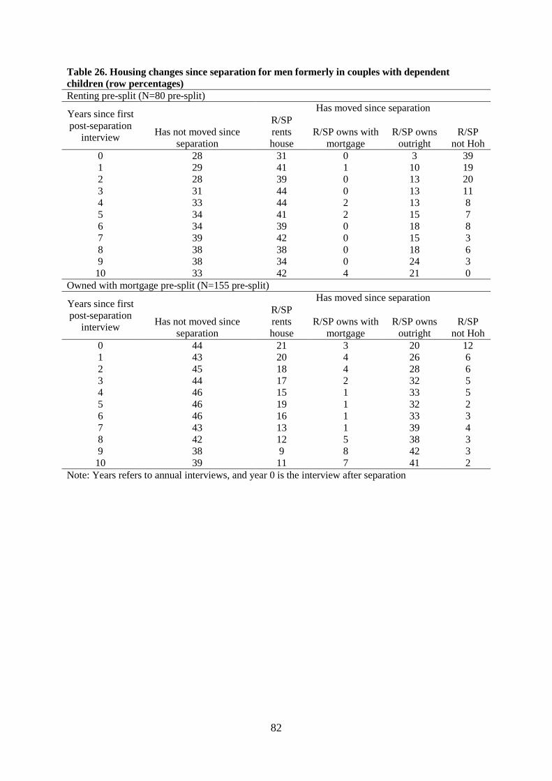
82

Table 26. Housing changes since separation for men formerly in couples with dependent children (row percentages) Renting pre-split (N=80 pre-split)

Years since first post-separation

interview Has not moved since separation

Has moved since separation R/SP rents house

R/SP owns with mortgage

R/SP owns outright

R/SP not Hoh

0 28 31 0 3 39 1 29 41 1 10 19 2 28 39 0 13 20 3 31 44 0 13 11 4 33 44 2 13 8 5 34 41 2 15 7 6 34 39 0 18 8 7 39 42 0 15 3 8 38 38 0 18 6 9 38 34 0 24 3

10 33 42 4 21 0 Owned with mortgage pre-split (N=155 pre-split)

Years since first post-separation

interview Has not moved since separation

Has moved since separation R/SP rents house

R/SP owns with mortgage

R/SP owns outright

R/SP not Hoh

0 44 21 3 20 12 1 43 20 4 26 6 2 45 18 4 28 6 3 44 17 2 32 5 4 46 15 1 33 5 5 46 19 1 32 2 6 46 16 1 33 3 7 43 13 1 39 4 8 42 12 5 38 3 9 38 9 8 42 3

10 39 11 7 41 2 Note: Years refers to annual interviews, and year 0 is the interview after separation

83

Table 27. Housing changes since separation for women formerly in couples with no dependent children but who had dependent children earlier (row percentages) Owned with mortgage pre-split (N=41 pre-split)

Years since first post-separation

interview Has not moved since separation

Has moved since separation R/SP rents house

R/SP owns with mortgage

R/SP owns outright

R/SP not Hoh

0 51 24 7 15 2 1 49 22 11 19 0 2 49 17 14 17 3 3 47 18 12 21 3 4 47 20 13 20 0 5 45 16 13 23 3 6 45 16 13 23 3 7 41 15 19 22 4 8 35 22 17 26 0 9 33 19 10 33 5

10 25 25 25 25 0 Note: Years refers to annual interviews, and year 0 is the interview after separation Table 28. Housing changes since separation for men formerly in couples with no dependent children but who had dependent children earlier Owned with mortgage pre-split (N= 44 pre-split

Years since first post-separation

interview Has not moved since separation

Has moved since separation R/SP rents house

R/SP owns with mortgage

R/SP owns outright

R/SP not Hoh

0 57 27 7 5 5 1 54 18 10 18 0 2 55 11 11 24 0 3 56 12 12 21 0 4 56 9 19 16 0 5 60 10 13 17 0 6 57 11 18 14 0 7 61 7 18 14 0 8 71 8 13 8 0 9 71 8 17 4 0

10 71 10 14 5 0 Note: Years refers to annual interviews, and year 0 is the interview after separation

84

Table 29. Housing changes since separation for women formerly in couples with no dependent children (row percentages) Renting pre-split (N=56 pre-split)

Years since first post-separation

interview Has not moved since separation

Has moved since separation R/SP rents house

R/SP owns with mortgage

R/SP owns outright

R/SP not Hoh

0 21 25 0 16 38 1 24 33 0 16 27 2 24 36 0 24 16 3 24 36 0 26 14 4 21 37 0 34 8 5 18 38 0 44 0 6 19 38 0 41 3 7 11 44 0 44 0 8 14 41 0 41 5 9 17 28 0 50 6

10 15 38 0 46 0 Owned with mortgage pre-split (N=114 pre-split)

Years since first post-separation

interview Has not moved since separation

Has moved since separation R/SP rents house

R/SP owns with mortgage

R/SP owns outright

R/SP not Hoh

0 37 20 3 24 17 1 38 18 4 26 14 2 40 13 4 37 6 3 39 10 6 39 6 4 39 8 6 45 2 5 38 8 6 46 3 6 36 7 5 49 3 7 37 4 7 50 1 8 38 7 10 45 0 9 40 10 6 42 2

10 49 7 5 35 5 Not the head of household pre-split (N=82 pre-split)

Years since first post-separation

interview Has not moved since separation

Has moved since separation R/SP rents house

R/SP owns with mortgage

R/SP owns outright

R/SP not Hoh

0 28 18 1 4 49 1 25 25 5 8 38 2 27 24 3 14 32 3 28 25 2 21 25 4 27 25 0 29 18 5 24 28 0 33 15 6 22 19 3 41 16 7 21 26 3 44 6 8 21 29 0 36 14 9 21 33 0 38 8

10 22 22 0 48 9 Note: Years refers to annual interviews, and year 0 is the interview after separation

85

Table 30. Housing changes since separation for men formerly in couples with no dependent children (row percentages) Renting pre-split (N=60 pre-split)

Years since first post-separation

interview Has not moved since separation

Has moved since separation R/SP rents house

R/SP owns with mortgage

R/SP owns outright

R/SP not Hoh

0 40 25 3 5 27 1 42 25 2 13 17 2 37 26 2 24 11 3 38 28 3 25 8 4 30 36 0 33 0 5 28 24 0 44 4 6 23 32 5 41 0 7 26 21 0 53 0 8 28 28 0 44 0 9 36 29 0 36 0

10 33 25 0 42 0 Owned with mortgage pre-split (N=97 pre-split)

Years since first post-separation

interview Has not moved since separation

Has moved since separation R/SP rents house

R/SP owns with mortgage

R/SP owns outright

R/SP not Hoh

0 51 12 1 20 16 1 49 12 1 25 12 2 46 10 3 30 11 3 49 7 1 32 11 4 51 7 1 34 6 5 51 8 2 33 6 6 51 14 4 28 4 7 54 11 0 30 4 8 49 7 2 37 5 9 51 8 0 38 3

10 50 11 0 36 3 Not the head of household pre-split (N=58 pre-split)

Years since first post-separation

interview Has not moved since separation

Has moved since separation R/SP rents house

R/SP owns with mortgage

R/SP owns outright

R/SP not Hoh

0 31 21 2 7 40 1 34 18 0 14 34 2 32 25 0 13 30 3 32 19 0 19 30 4 29 18 0 24 29 5 31 34 0 19 16 6 33 37 0 17 13 7 37 26 0 26 11 8 42 29 0 17 13 9 45 14 0 23 18

10 45 25 0 20 10 Note: Years refers to annual interviews, and year 0 is the interview after separation

86

Table 31. Estimated coefficients of an OLS regression of the absolute change in GHQ-12 (0-36 scale) measured from 2 interviews before separation with only income and time since separation as covariates

Women with dependent children in the interview before separation

Constant 2.614**

2.609** 2.618** 1 year after first observed as single -2.331**

-2.322** -2.343**

2 years after first observed as single -2.948**

-2.931** -2.970**

3 years after first observed as single -3.412**

-3.391** -3.440**

4+ years after first observed as single -4.210**

-4.215** -4.192**

4+ years after first observed as single, slope 0.035

0.041 0.025

Proportionate Change in Net Household BHC Income

-0.343+

-0.082

Proportionate Change in Net Household AHC Income

-0.045

0.087

Number of observations 2362 2362 2362 2362 2362

R-squared 0.025 0.002 0 0.026 0.026

Men with dependent children in the interview before separation

Constant 3.966**

4.042** 4.000** 1 year after first observed as single -3.938**

-3.914** -3.908**

2 years after first observed as single -4.570**

-4.510** -4.513**

3 years after first observed as single -3.871**

-3.823** -3.838**

4+ years after first observed as single -4.036**

-3.989** -4.013**

4+ years after first observed as single, slope 0.049

0.052 0.052

Proportionate Change in Net Household BHC Income

-0.296+

-0.222

Proportionate Change in Net Household AHC Income

-0.165

-0.111

Number of observations 1480 1480 1480 1480 1480

R-squared 0.031 0.002 0.001 0.032 0.031

87

Table 32. Estimated coefficients of an OLS regression of the absolute change in GHQ-12 (0-36 scale) measured from 2 interviews prior to separation with only income and time since separation as covariates

Women without dependent children in the interview before separation, had children earlier

Women without dependent children in the interview before separation, no children earlier

Constant 3.052** -1.141** -1.227** 2.840** 3.021** 2.062** 0.720** 0.733** 2.057** 2.050** 1 year after first observed as single -4.070**

-4.165** -4.104** -1.885*

-1.910* -1.897*

2 years after first observed as single -3.632*

-3.513* -3.614* -1.168

-1.217 -1.204

3 years after first observed as single -4.794**

-4.566** -4.710** -1.428+

-1.548* -1.520*

4+ years after first observed as single -6.495**

-5.750* -5.906* -1.744

-1.837 -1.857

4+ years after first observed as single, slope 0.111

0.112 0.073 0.036

0.036 0.042

Proportionate Change in Net Household BHC Income

-1.584**

-1.442**

0.326

0.365

Proportionate Change in Net Household AHC Income

-0.260**

-0.228*

0.149

0.164

Number of observations 529 529 529 529 529 1286 1286 1286 1286 1286

R-squared 0.04 0.047 0.016 0.077 0.051 0.004 0.002 0.001 0.007 0.006

Men without dependent children in the interview before

Separation, had children earlier Men without dependent children in the interview

before separation, no children earlier

Constant 2.865** 0.739* 0.757* 2.827** 2.779** 2.679** 1.174** 1.175** 2.679** 2.679** 1 year after first observed as single -2.810*

-2.606* -2.667* -1.908**

-1.910** -1.909**

2 years after first observed as single -2.095

-1.623 -1.681 -2.467**

-2.471** -2.469**

3 years after first observed as single -3.324**

-2.897** -2.747* -1.243*

-1.249* -1.246*

4+ years after first observed as single -5.359**

-4.983* -4.430* -3.953**

-3.954** -3.952**

4+ years after first observed as single, slope 0.28

0.310+ 0.258 0.237*

0.236* 0.236*

Proportionate Change in Net Household BHC Income

-2.320**

-2.281**

-0.004

0.023

Proportionate Change in Net Household AHC Income

-2.259**

-2.187**

-0.005

0.009

Number of observations 486 486 486 486 486 1235 1235 1235 1235 1235

R-squared 0.023 0.074 0.078 0.093 0.095 0.018 0 0 0.018 0.018

88

Table 33. Family living arrangements at the interviews before and after a separation

Children Children-year observations

No. % No. % Living with both parents at interview before parental separation, living with mother after separation

422 42% 5055 46%

Living with both parents at interview before parental separation, living with father after separation

48 5% 536 5%

Living with one parent at interview before parental separation, living with mother after separation

459 46% 4759 43%

Living with one parent at interview before parental separation, living with father after separation

47 5% 511 5%

Rest 21 2% 248 2% Total 997 100% 11109 100%

Table 34. Number of child-year observations

Years since first observed as single

Living with both parents at interview before parental separation, with mother

after separation

Living with father after separation

Living with one parent at interview before parental separation, with mother

after separation -2 317 62 232 -1 292 55 191 0 260 53 202 1 244 45 173 2 216 43 146 3 195 33 104 4 178 26 95 5 156 21 78

89

Figure 1. Median net equivalised household income before and after separation

200

300

400

500

600

£ pe

r wee

k

-2 0 2 4 6 8 10Years since separation

women, dependent children at t=-1 women, no dependent children at t=-1 but earlier

women, no dependent children at t=-1 or earlier men, dependent children at t=-1

men, no dependent children at t=-1 but earlier men, no dependent children at t=-1 or earlier

Note: Year refers to annual interviews and 0 refers to the interview right after separation

Median net equivalised (bhc) household income

200

300

400

500

600

£ pe

r wee

k

-2 0 2 4 6 8 10Years since separation

women, dependent children at t=-1 women, no dependent children at t=-1 but earlier

women, no dependent children at t=-1 or earlier men, dependent children at t=-1

men, no dependent children at t=-1 but earlier men, no dependent children at t=-1 or earlier

Note: Year refers to annual interviews and 0 refers to the interview right after separation

Median net equivalised (ahc) household income

90

Figure 2. Median change in net equivalised household income since separation

-100

-50

050

100

150

£ pe

r wee

k

-2 0 2 4 6 8 10Years since separation

women, dependent children at t=-1 women, no dependent children at t=-1 but earlier

women, no dependent children at t=-1 or earlier men, dependent children at t=-1

men, no dependent children at t=-1 but earlier men, no dependent children at t=-1 or earlier

Note: Year refers to annual interviews and 0 refers to the interview right after separation

Median absolute change in net equivalised (bhc) household income

-200

-100

010

020

0£

per w

eek

-2 0 2 4 6 8 10Years since separation

women, dependent children at t=-1 women, no dependent children at t=-1 but earlier

women, no dependent children at t=-1 or earlier men, dependent children at t=-1

men, no dependent children at t=-1 but earlier men, no dependent children at t=-1 or earlier

Note: Year refers to annual interviews and 0 refers to the interview right after separation

Median absolute change in net equivalised (ahc) household income

91

Figure 3. Median percentage change in net equivalised household income since separation

-50

050

100

%

-2 0 2 4 6 8 10Years since separation

women, dependent children at t=-1 women, no dependent children at t=-1 but earlier

women, no dependent children at t=-1 or earlier men, dependent children at t=-1

men, no dependent children at t=-1 but earlier men, no dependent children at t=-1 or earlier

Note: Year refers to annual interviews and 0 refers to the interview right after separation

Median %age change in net equivalised (bhc) household income

-50

050

100

%

-2 0 2 4 6 8 10Years since separation

women, dependent children at t=-1 women, no dependent children at t=-1 but earlier

women, no dependent children at t=-1 or earlier men, dependent children at t=-1

men, no dependent children at t=-1 but earlier men, no dependent children at t=-1 or earlier

Note: Year refers to annual interviews and 0 refers to the interview right after separation

Median %age change in net equivalised (ahc) household income

92

Figure 4. Median net equivalised household income before and after separation, by whether initially above or below median income

200

400

600

£ pe

r wee

k

-2 0 2 4 6 8 10Years since separation

women, dependent children at t=-1

200

400

600

£ pe

r wee

k-2 0 2 4 6 8 10

Years since separation

women, no dependent children at t=-1 but earlier

200

400

600

£ pe

r wee

k

-2 0 2 4 6 8 10Years since separation

women, no dependent children at t=-1 or earlier

200

400

600

£ pe

r wee

k

-2 0 2 4 6 8 10Years since separation

men, dependent children at t=-1

200

400

600

£ pe

r wee

k

-2 0 2 4 6 8 10Years since separation

men, no dependent children at t=-1 but earlier

200

400

600

£ pe

r wee

k-2 0 2 4 6 8 10

Years since separation

men, no dependent children at t=-1 or earlier

Note: Year refers to annual interviews and 0 refers to the interview right after separation

Median net equivalised (bhc) household income

income above median income below median

200

400

600

£ pe

r wee

k

-2 0 2 4 6 8 10Years since separation

women, dependent children at t=-1

200

400

600

£ pe

r wee

k

-2 0 2 4 6 8 10Years since separation

women, no dependent children at t=-1 but earlier

200

400

600

£ pe

r wee

k

-2 0 2 4 6 8 10Years since separation

women, no dependent children at t=-1 or earlier

200

400

600

£ pe

r wee

k

-2 0 2 4 6 8 10Years since separation

men, dependent children at t=-1

200

400

600

£ pe

r wee

k

-2 0 2 4 6 8 10Years since separation

men, no dependent children at t=-1 but earlier

200

400

600

£ pe

r wee

k

-2 0 2 4 6 8 10Years since separation

men, no dependent children at t=-1 or earlier

Note: Year refers to annual interviews and 0 refers to the interview right after separation

Median net equivalised (ahc) household income

income above median income below median

93

Figure 5. Median change in net equivalised household income since separation, by whether initially above or below median income

-100

010

020

030

0£

per w

eek

-2 0 2 4 6 8 10Years since separation

women, dependent children at t=-1

-100

010

0200

300

£ pe

r wee

k-2 0 2 4 6 8 10

Years since separation

women, no dependent children at t=-1 but earlier

-100

010

020

030

0£

per w

eek

-2 0 2 4 6 8 10Years since separation

women, no dependent children at t=-1 or earlier

-100

010

020

030

0£

per w

eek

-2 0 2 4 6 8 10Years since separation

men, dependent children at t=-1

-100

010

020

030

0£

per w

eek

-2 0 2 4 6 8 10Years since separation

men, no dependent children at t=-1 but earlier

-100

010

020

030

0£

per w

eek

-2 0 2 4 6 8 10Years since separation

men, no dependent children at t=-1 or earlier

Note: Year refers to annual interviews and 0 refers to the interview right after separation

Median absolute change in net equivalised (bhc) household income

income above median income below median

-100

010

020

030

0£

per w

eek

-2 0 2 4 6 8 10Years since separation

women, dependent children at t=-1

-100

010

020

030

0£

per w

eek

-2 0 2 4 6 8 10Years since separation

women, no dependent children at t=-1 but earlier

-100

010

020

030

0£

per w

eek

-2 0 2 4 6 8 10Years since separation

women, no dependent children at t=-1 or earlier

-100

010

020

030

0£

per w

eek

-2 0 2 4 6 8 10Years since separation

men, dependent children at t=-1

-100

010

020

030

0£

per w

eek

-2 0 2 4 6 8 10Years since separation

men, no dependent children at t=-1 but earlier

-100

010

020

030

0£

per w

eek

-2 0 2 4 6 8 10Years since separation

men, no dependent children at t=-1 or earlier

Note: Year refers to annual interviews and 0 refers to the interview right after separation

Median absolute change in net equivalised (ahc) household income

income above median income below median

94

Figure 6. Median percentage change in net equivalised household income since separation, by whether initially above or below median income

-50

050

100

150

%

-2 0 2 4 6 8 10Years since separation

women, dependent children at t=-1

-50

050

100

150

%-2 0 2 4 6 8 10

Years since separation

women, no dependent children at t=-1 but earlier

-50

050

100

150

%

-2 0 2 4 6 8 10Years since separation

women, no dependent children at t=-1 or earlier

-50

050

100

150

%

-2 0 2 4 6 8 10Years since separation

men, dependent children at t=-1

-50

050

100

150

%

-2 0 2 4 6 8 10Years since separation

men, no dependent children at t=-1 but earlier

-50

050

100

150

%-2 0 2 4 6 8 10

Years since separation

men, no dependent children at t=-1 or earlier

Note: Year refers to annual interviews and 0 refers to the interview right after separation

Median % change in net equivalised (bhc) household income

income above median income below median

-50

050

100

150

%

-2 0 2 4 6 8 10Years since separation

women, dependent children at t=-1

-50

050

100

150

%

-2 0 2 4 6 8 10Years since separation

women, no dependent children at t=-1 but earlier

-50

050

100

150

%

-2 0 2 4 6 8 10Years since separation

women, no dependent children at t=-1 or earlier

-50

050

100

150

%

-2 0 2 4 6 8 10Years since separation

men, dependent children at t=-1

-50

050

100

150

%

-2 0 2 4 6 8 10Years since separation

men, no dependent children at t=-1 but earlier

-50

050

100

150

%

-2 0 2 4 6 8 10Years since separation

men, no dependent children at t=-1 or earlier

Note: Year refers to annual interviews and 0 refers to the interview right after separation

Median % change in net equivalised (ahc) household income

income above median income below median

95

Figure 7. Percentage change in net equivalised household income around separation, by pre-separation income

-100

-50

050

100

% c

hang

e at

t=0

from

t=-2

0 200 400 600 800bhc income at t=-2

bandwidth = .8

women, dependent children at t=-1, size(small)

-100

-50

050

100

% c

hang

e at

t=0

from

t=-2

0 200 400 600 800bhc income at t=-2

bandwidth = .8

women, no dependent children at t=-1 but earlier, size(small)

-100

-50

050

100

% c

hang

e at

t=0

from

t=-2

0 200 400 600 800bhc income at t=-2

bandwidth = .8

women, no dependent children at t=-1 or earlier, size(small)

-100

-50

050

100

% c

hang

e at

t=0

from

t=-2

0 200 400 600 800bhc income at t=-2

bandwidth = .8

men, dependent children at t=-1, size(small)

-100

-50

050

100

% c

hang

e at

t=0

from

t=-2

0 200 400 600 800bhc income at t=-2

bandwidth = .8

men, no dependent children at t=-1 but earlier, size(small)

-100

-50

050

100

% c

hang

e at

t=0

from

t=-2

0 200 400 600 800bhc income at t=-2

bandwidth = .8

men, no dependent children at t=-1 or earlier, size(small)

Note: Year refers to annual interviews and 0 refers to the interview right after separation

-100

-50

050

100

% c

hang

e at

t=0

from

t=-2

0 200 400 600 800ahc income at t=-2

bandwidth = .8

women, dependent children at t=-1, size(small)

-100

-50

050

% c

hang

e at

t=0

from

t=-2

0 200 400 600 800ahc income at t=-2

bandwidth = .8

women, no dependent children at t=-1 but earlier, size(small)

-100

-50

050

100

% c

hang

e at

t=0

from

t=-2

0 200 400 600 800ahc income at t=-2

bandwidth = .8

women, no dependent children at t=-1 or earlier, size(small)

-100

-50

050

100

% c

hang

e at

t=0

from

t=-2

0 200 400 600 800ahc income at t=-2

bandwidth = .8

men, dependent children at t=-1, size(small)

-100

-50

050

100

% c

hang

e at

t=0

from

t=-2

0 200 400 600 800ahc income at t=-2

bandwidth = .8

men, no dependent children at t=-1 but earlier, size(small)

-100

-50

050

100

% c

hang

e at

t=0

from

t=-2

0 200 400 600 800ahc income at t=-2

bandwidth = .8

men, no dependent children at t=-1 or earlier, size(small)

Note: Year refers to annual interviews and 0 refers to the interview right after separation

96

Figure 8. Proportion of adults in relative income poverty before and after separation

0.1

.2.3

.4

-2 -1 0 1 2 3 4 5 6 7 8 9 10Years since separation

women, dependent children at t=-1 women, no dependent children at t=-1 but earlier

women, no dependent children at t=-1 or earlier men, dependent children at t=-1

men, no dependent children at t=-1 but earlier men, no dependent children at t=-1 or earlier

Note: Year refers to annual interviews and 0 refers to the interview right after separation

Proportion bhc poor

0.1

.2.3

.4

-2 -1 0 1 2 3 4 5 6 7 8 9 10Years since separation

women, dependent children at t=-1 women, no dependent children at t=-1 but earlier

women, no dependent children at t=-1 or earlier men, dependent children at t=-1

men, no dependent children at t=-1 but earlier men, no dependent children at t=-1 or earlier

Note: Year refers to annual interviews and 0 refers to the interview right after separation

Proportion ahc poor

97

Figure 9. Proportion of adults poor before and after separation, by whether above or below median before separation

0.2

.4.6

-2 -1 0 1 2 3 4 5 6 7 8 9 10Years since separation

women, dep. kids at t=-1, below median women, dep. kids at t=-1, above median

women, no dep. kids at t=-1 but earlier, below medianwomen, no dep. kids at t=-1 but earlier, above median

women, no dep. kids ever, below median women, no dep. kids ever, above median

Note: Year refers to annual interviews and 0 refers to the interview right after separation

Proportion bhc poor among women

0.1

.2.3

.4

-2 -1 0 1 2 3 4 5 6 7 8 9 10Years since separation

men, dep. kids at t=-1, below median men, dep. kids at t=-1, above median

men, no dep. kids at t=-1 but earlier, below medianmen, no dep. kids at t=-1 but earlier, above median

men, no dep. kids ever, below median men, no dep. kids ever, above median

Note: Year refers to annual interviews and 0 refers to the interview right after separation

Proportion bhc poor among men

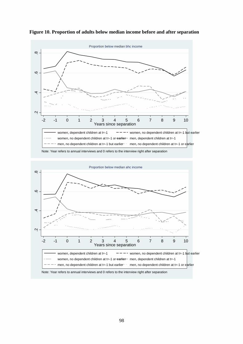
98

Figure 10. Proportion of adults below median income before and after separation

.2.4

.6.8

-2 -1 0 1 2 3 4 5 6 7 8 9 10Years since separation

women, dependent children at t=-1 women, no dependent children at t=-1 but earlier

women, no dependent children at t=-1 or earlier men, dependent children at t=-1

men, no dependent children at t=-1 but earlier men, no dependent children at t=-1 or earlier

Note: Year refers to annual interviews and 0 refers to the interview right after separation

Proportion below median bhc income

.2.4

.6.8

-2 -1 0 1 2 3 4 5 6 7 8 9 10Years since separation

women, dependent children at t=-1 women, no dependent children at t=-1 but earlier

women, no dependent children at t=-1 or earlier men, dependent children at t=-1

men, no dependent children at t=-1 but earlier men, no dependent children at t=-1 or earlier

Note: Year refers to annual interviews and 0 refers to the interview right after separation

Proportion below median ahc income

99

Figure 11. Level of and change in material deprivation amongst adults before and after separation

-.20

.2.4

-2 -1 0 1 2 3 4 5 6 7 8 9 10Years since separation

women, dependent children at t=-1 women, no dependent children at t=-1 but earlier

women, no dependent children at t=-1 or earlier men, dependent children at t=-1

men, no dependent children at t=-1 but earlier men, no dependent children at t=-1 or earlier

Note: Year refers to annual interviews and 0 refers to the interview right after separation

Mean composite deprivation score

-.20

.2.4

-2 -1 0 1 2 3 4 5 6 7 8 9 10Years since separation

women, dependent children at t=-1 women, no dependent children at t=-1 but earlier

women, no dependent children at t=-1 or earlier men, dependent children at t=-1

men, no dependent children at t=-1 but earlier men, no dependent children at t=-1 or earlier

Note: Year refers to annual interviews and 0 refers to the interview right after separation

Mean absolute change in composite deprivation scoreSince t=-2

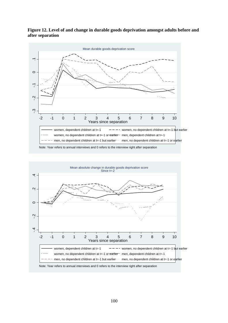
100

Figure 12. Level of and change in durable goods deprivation amongst adults before and after separation

-.3-.2

-.10

.1

-2 -1 0 1 2 3 4 5 6 7 8 9 10Years since separation

women, dependent children at t=-1 women, no dependent children at t=-1 but earlier

women, no dependent children at t=-1 or earlier men, dependent children at t=-1

men, no dependent children at t=-1 but earlier men, no dependent children at t=-1 or earlier

Note: Year refers to annual interviews and 0 refers to the interview right after separation

Mean durable goods deprivation score

-.4-.2

0.2

.4

-2 -1 0 1 2 3 4 5 6 7 8 9 10Years since separation

women, dependent children at t=-1 women, no dependent children at t=-1 but earlier

women, no dependent children at t=-1 or earlier men, dependent children at t=-1

men, no dependent children at t=-1 but earlier men, no dependent children at t=-1 or earlier

Note: Year refers to annual interviews and 0 refers to the interview right after separation

Mean absolute change in durable goods deprivation scoreSince t=-2

101

Figure 13. Level of and change in daily living deprivation amongst adults before and after separation

-.20

.2.4

.6

-2 -1 0 1 2 3 4 5 6 7 8 9 10Years since separation

women, dependent children at t=-1 women, no dependent children at t=-1 but earlier

women, no dependent children at t=-1 or earlier men, dependent children at t=-1

men, no dependent children at t=-1 but earlier men, no dependent children at t=-1 or earlier

Note: Year refers to annual interviews and 0 refers to the interview right after separation

Mean daily living deprivation score

-.4-.2

0.2

.4

-2 -1 0 1 2 3 4 5 6 7 8 9 10Years since separation

women, dependent children at t=-1 women, no dependent children at t=-1 but earlier

women, no dependent children at t=-1 or earlier men, dependent children at t=-1

men, no dependent children at t=-1 but earlier men, no dependent children at t=-1 or earlier

Note: Year refers to annual interviews and 0 refers to the interview right after separation

Mean absolute change in daily Living deprivation scoreSince t=-2

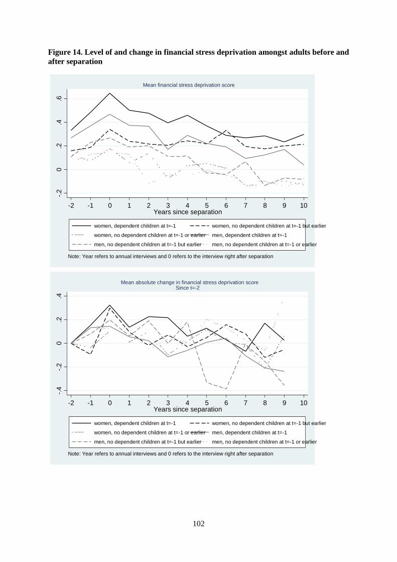
102

Figure 14. Level of and change in financial stress deprivation amongst adults before and after separation

-.20

.2.4

.6

-2 -1 0 1 2 3 4 5 6 7 8 9 10Years since separation

women, dependent children at t=-1 women, no dependent children at t=-1 but earlier

women, no dependent children at t=-1 or earlier men, dependent children at t=-1

men, no dependent children at t=-1 but earlier men, no dependent children at t=-1 or earlier

Note: Year refers to annual interviews and 0 refers to the interview right after separation

Mean financial stress deprivation score

-.4-.2

0.2

.4

-2 -1 0 1 2 3 4 5 6 7 8 9 10Years since separation

women, dependent children at t=-1 women, no dependent children at t=-1 but earlier

women, no dependent children at t=-1 or earlier men, dependent children at t=-1

men, no dependent children at t=-1 but earlier men, no dependent children at t=-1 or earlier

Note: Year refers to annual interviews and 0 refers to the interview right after separation

Mean absolute change in financial stress deprivation scoreSince t=-2

103

Figure 15. Proportion of adults finding their financial situation difficult before and after separation

05

1015

2025

30%

-2-1 0 1 2 3 4 5 6 7 8 910

women, dependent children at t=-1

05

1015

2025

30%

-2 -1 0 1 2 3 4 5 6 7 8 9 10

women, no dependent children at t=-1 but earlier

05

1015

2025

30%

-2-1 0 1 2 3 4 5 6 7 8 910

women, no dependent children at t=-1 or earlier

05

1015

2025

30%

-2-1 0 1 2 3 4 5 6 7 8 910

men, dependent children at t=-1

05

1015

2025

30%

-2-1 0 1 2 3 4 5 6 7 8 910

men, no dependent children at t=-1 but earlier

05

1015

2025

30%

-2 -1 0 1 2 3 4 5 6 7 8 910

men, no dependent children at t=-1 or earlier

Note: Year refers to annual interviews and 0 refers to the interview right after separation

Self-reported financial situation over years since separation

Finding it quite difficult Finding it very difficult

104

Figure 16. Level of and change in mental distress before and after separation

1012

1416

-2 0 2 4 6 8 10Years since separation

women, dependent children at t=-1 women, no dependent children at t=-1 but earlier

women, no dependent children at t=-1 or earlier men, dependent children at t=-1

men, no dependent children at t=-1 but earlier men, no dependent children at t=-1 or earlier

Note: Year refers to annual interviews and 0 refers to the interview right after separation

Mean mental distress (GHQ-12, 0-36 scale)since 2 years prior to separation

-4-2

02

4

-2 0 2 4 6 8 10Years since separation

women, dependent children at t=-1 women, no dependent children at t=-1 but earlier

women, no dependent children at t=-1 or earlier men, dependent children at t=-1

men, no dependent children at t=-1 but earlier men, no dependent children at t=-1 or earlier

Note: Year refers to annual interviews and 0 refers to the interview right after separation

Mean absolute change in mental distress (GHQ-12, 0-36 scale)since 2 years prior to separation

105

Figure 17. Proportion of adults with caseness score of 4 or more before and after separation

0.1

.2.3

.4.5

0.1

.2.3

.4.5

0.1

.2.3

.4.5

-2 -1 0 1 2 3 4 5 6 7 8 9 10 -2 -1 0 1 2 3 4 5 6 7 8 9 10

-2 -1 0 1 2 3 4 5 6 7 8 9 10 -2 -1 0 1 2 3 4 5 6 7 8 9 10

-2 -1 0 1 2 3 4 5 6 7 8 9 10 -2 -1 0 1 2 3 4 5 6 7 8 9 10

women, dep. kids at t=-1 women, no dep. kids at t=-1 but earlier

women, no dep. kids at t=-1 or earlier men, dep. kids at t=-1

men, no dep. kids at t=-1 but earlier men, no dep. kids at t=-1 or earlier

Pro

porti

on w

ith G

HQ

-12

Cas

enes

s sc

ore

of 4

to 1

2

Note: 0 refers to interview after separation

106

Figure 18. Level of and change in overall life satisfaction amongst adults before and after separation

44.

55

5.5

-2 -1 0 1 2 3 4 5 6 7 8 9 10Years since separation

women, dependent children at t=-1 women, no dependent children at t=-1 but earlier

women, no dependent children at t=-1 or earlier men, dependent children at t=-1

men, no dependent children at t=-1 but earlier men, no dependent children at t=-1 or earlier

Note: Year refers to annual interviews and 0 refers to the interview right after separation

Mean overall life satisfaction (0-7 scale)

-1-.5

0.5

1

-2 -1 0 1 2 3 4 5 6 7 8 9 10Years since separation

women, dependent children at t=-1 women, no dependent children at t=-1 but earlier

women, no dependent children at t=-1 or earlier men, dependent children at t=-1

men, no dependent children at t=-1 but earlier men, no dependent children at t=-1 or earlier

Note: Year refers to annual interviews and 0 refers to the interview right after separation

Mean absolute change overall life satisfaction (0-7 scale)Since t=-2

107

Figure 19. Level of net equivalised household income of children before and after separation

Figure 20. Change in net equivalised household income of children before and after separation

150

200

250

300

350

400

£ pe

r wee

k

-2 -1 0 1 2 3 4 5Years since parents separation

bhc

150

200

250

300

350

400

£ pe

r wee

k

-2 -1 0 1 2 3 4 5Years since parents separation

ahc

Note: Year refers to annual interviews and 0 refers to year after parents separation

Median net equivalised household income,of dependent children

Living with both parents at t-1, only mother at t=0

living with father at t=0

Living with only one parent at t-1, only mother at t=0

-50

050

100

150

£ pe

r wee

k

-2 -1 0 1 2 3 4 5Years since parents separation

bhc

-50

050

100

150

£ pe

r wee

k

-2 -1 0 1 2 3 4 5Years since parents separation

ahc

Note: Year refers to annual interviews and 0 refers to year after parents separation

Median absolute change innet equivalised household income,

of dependent children

Living with both parents at t-1, only mother at t=0

living with father at t=0

Living with only one parent at t-1, only mother at t=0

108

Figure 21. Median percentage change in net equivalised household income of children since separation

-20

020

40%

-2 -1 0 1 2 3 4 5Years since parents separation

bhc

-40

-20

020

40%

-2 -1 0 1 2 3 4 5Years since parents separation

ahc

Note: Year refers to annual interviews and 0 refers to year after parents separation

Median %age change innet equivalised household income,

of dependent children

Living with both parents at t-1, only mother at t=0

living with father at t=0

Living with only one parent at t-1, only mother at t=0

109

Figure 22. Median net equivalised household income of children who live with their mother after separation, before and after separation, by whether in above or below median income household before separation

200

300

400

500

£ pe

r wee

k

-2 -1 0 1 2 3 4 5Years since parents separation

Living with both parents year before separation, income above median

Living with only one parent year before separation, income above median

Living with both parents year before separation, income below median

Living with only one parent year before separation, income below median

Note: Year refers to annual interviews and 0 refers to year after parents separation

Median net equivalised (bhc) household incomedependent children, living with mother at separation

100

200

300

400

500

£ pe

r wee

k

-2 -1 0 1 2 3 4 5Years since parents separation

Living with both parents year before separation, income above median

Living with only one parent year before separation, income above median

Living with both parents year before separation, income below median

Living with only one parent year before separation, income below median

Note: Year refers to annual interviews and 0 refers to year after parents separation

Median net equivalised (ahc) household incomedependent children, living with mother at separation

110

Figure 23. Median change since separation in net equivalised household income of children who live with their mother after separation, by whether in above or below median income household before separation

-200

-100

010

0£

per w

eek

-2 -1 0 1 2 3 4 5Years since parents separation

Living with both parents year before separation, income above median

Living with only one parent year before separation, income above median

Living with both parents year before separation, income below median

Living with only one parent year before separation, income below median

Note: Year refers to annual interviews and 0 refers to year after parents separation

Median absolute change in net equivalised (bhc) household incomedependent children, living with mother at separation

-200

-100

010

0£

per w

eek

-2 -1 0 1 2 3 4 5Years since parents separation

Living with both parents year before separation, income above median

Living with only one parent year before separation, income above median

Living with both parents year before separation, income below median

Living with only one parent year before separation, income below median

Note: Year refers to annual interviews and 0 refers to year after parents separation

Median absolute change in net equivalised (ahc) household incomedependent children, living with mother at separation

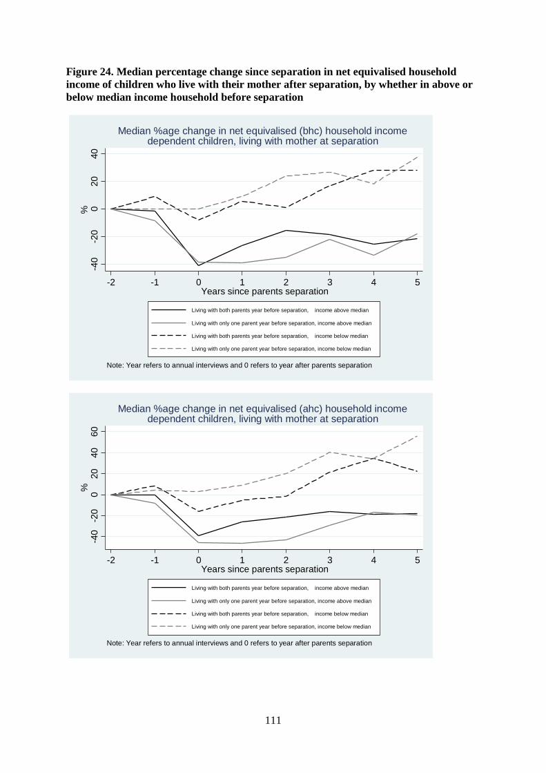
111

Figure 24. Median percentage change since separation in net equivalised household income of children who live with their mother after separation, by whether in above or below median income household before separation

-40

-20

020

40%

-2 -1 0 1 2 3 4 5Years since parents separation

Living with both parents year before separation, income above median

Living with only one parent year before separation, income above median

Living with both parents year before separation, income below median

Living with only one parent year before separation, income below median

Note: Year refers to annual interviews and 0 refers to year after parents separation

Median %age change in net equivalised (bhc) household incomedependent children, living with mother at separation

-40

-20

020

4060

%

-2 -1 0 1 2 3 4 5Years since parents separation

Living with both parents year before separation, income above median

Living with only one parent year before separation, income above median

Living with both parents year before separation, income below median

Living with only one parent year before separation, income below median

Note: Year refers to annual interviews and 0 refers to year after parents separation

Median %age change in net equivalised (ahc) household incomedependent children, living with mother at separation

112

Figure 25. Proportion of children in relative income poverty before and after separation

.1.2

.3.4

.5

-2 -1 0 1 2 3 4 5years since separation

Living with both parents at t-1, only mother at t=0Living with only one parent at t-1, only mother at t=0

Note: Year refers to annual interviews and 0 refers to year after parents separation

Proportion bhc poorDependent children

.1.2

.3.4

.5

-2 -1 0 1 2 3 4 5years since separation

Living with both parents at t-1, only mother at t=0Living with only one parent at t-1, only mother at t=0

Note: Year refers to annual interviews and 0 refers to year after parents separation

Proportion ahc poorDependent children

113

Figure 26. Proportion of children with below-median income before and after separation

.65

.7.7

5.8

.85

.9

-2 -1 0 1 2 3 4 5years since separation

Living with both parents at t-1, only mother at t=0Living with only one parent at t-1, only mother at t=0

Note: Year refers to annual interviews and 0 refers to year after parents separation

Proportion below median bhc incomeDependent children

.5.6

.7.8

.9

-2 -1 0 1 2 3 4 5years since separation

Living with both parents at t-1, only mother at t=0Living with only one parent at t-1, only mother at t=0

Note: Year refers to annual interviews and 0 refers to year after parents separation

Proportion below median ahc incomeDependent children

114

Figure 27. Level of and change in material deprivation score of children before and after separation

0.1

.2.3

.4

-2 -1 0 1 2 3 4 5years since separation

Living with both parents at t-1, only mother at t=0Living with only one parent at t-1, only mother at t=0

Note: Year refers to annual interviews and 0 refers to year after parents separation

Mean composite deprivation scoreDependent children

0.0

5.1

.15

.2.2

5

-2 -1 0 1 2 3 4 5years since separation

Living with both parents at t-1, only mother at t=0Living with only one parent at t-1, only mother at t=0

Note: Year refers to annual interviews and 0 refers to year after parents separation

Mean absolute change in composite deprivation scoreSince 2 years prior to separation

Dependent children

115

Annex A. Previous research on effects of partnership formation and dissolution on economic circumstances and well-being. Authors Data Details of Analysis Main statistics presented Economic impacts of separation (income changes) Poortman, 2000

Dutch Socioeconomic Panel (SEP), 1984-1995

- Split: Measured over 1 year period, transition from married or cohabiting to living alone. Those widowed, or splitting up from homosexual relationships are excluded. Also exclude those who remarried (or cohabited) within a year of separation. - Income: Disposable household income (represents financial situation after redistribution) and labour market income. Adjusted income (equivalence scale by Schiepers et al (1993)) and unadjusted income. - Analysis: Descriptive analysis of changes in income. Multivariate analysis to explore what percentage of the sex difference can be attributed to differences in human capital and presence of children (focusing on changes in adjusted disposable income). Regression of natural logarithm of post-separation disposable income for men and women together, and then separately for each sex. Decomposition (Oxaca, 1973) used to test how much sex difference can be explained by differences in human capital and children.

- Mean pre-separation disposable household income compared with a) mean post-separation labour market income and b) mean post-separation disposable household income, for both men and women, and using unadjusted and adjusted incomes, weighted. (Table 2) - Distribution of relative change in unadjusted and adjusted disposable household income for men and women (calculated as [[post-separation income – pre-separation income]/pre-separation income]*100%). (Fig. 1) - Regression of natural logarithm of adjusted post-separation disposable income on independent variables (men and women together. (Table 4) - Regression of natural logarithm of adjusted post-separation disposable income on independent variables, men and women separately. (Table 5)

Aassve et al, 2007

ECHP (1994-2001) Welfare clusters: Liberal countries (UK and Ireland);

- Split: Married in a given year, separated/divorced in following year and reporting to live in separate households. - Income: Conventional income/poverty: Household net equivalised income, adjusted using OECD modified equivalence scale. Different poverty thresholds (50%, 60% and 70%). Relative income: Fuzzy Monetary indicator.

- Average Treatment Effect of marital dissolution on poverty entry rate for different poverty thresholds, by gender, presence of children and welfare regime. (Table 3) (NB those already poor prior to split excluded from this analysis)

116

Authors Data Details of Analysis Main statistics presented Social Democratic countries (Finland and Denmark); Conservative countries (Belgium, Netherlands, France and Austria); and Mediterranean countries (Italy, Spain, Portugal, and Greece).

Deprivation index measure: (1) basic non-monetary deprivation (basic lifestyle deprivation); (2) secondary non-monetary deprivation (secondary lifestyle deprivation); (3) lack of housing facilities; (4) housing deterioration; (5) environmental problems. - Analysis: Use propensity score matching combined with Difference-in-differences estimator to control for selection bias. Use different measures of economic well-being (conventional income/poverty measures, Fuzzy Monetary indicator, Deprivation indices).

- Average Treatment Effect of marital dissolution on relative income (FM indicator), by gender, presence of children and welfare regime. (Table 4) - Average Treatment Effect of marital dissolution on total deprivation by gender, presence of children and welfare regime. (Table 5) - Average Treatment Effect of marital dissolution on basic lifestyle deprivation by gender, presence of children and welfare regime. (Table 6) - Average Treatment Effect of marital dissolution on secondary lifestyle deprivation by gender, presence of children and welfare regime. (Table 7)

Andreß et al, 2006

Belgium: PSBH, 1992-2002; Germany: GSOEP, 1984-1999; Great Britain: BHPS, 1991-2001; Italy: SHIW, 1987-2002; Sweden: HUS, 1984-1998

- Split: Married or cohabiting at t–1 and separated1 at t. Data on at least one partner must be available at t–1 (before separation) and t (after separation). Ages 18-60. First split in panel. - Income: Monthly disposable household income, adjusted using formula: household income/[size0.5] - Analysis: Descriptive analysis of changes in median adjusted household income before and after separation for men and women. Multivariate models of household income as function of country- and gender-specific characteristics (excluding Italy). RE and FE estimates. 1Focus on separations rather than divorce for married couples.

- Median adjusted household income t–5 to t+5 for men and women in each country. (Fig. 1) - Percentage change of adjusted household income for separated men and women in each country (t–1 to t). (Fig. 2) - Estimated changes in adjusted household income (separation effect for men and women, country differences for women, gender difference between countries, income trend after separation for women, years to gain pre-separation income, being in employment, caring for children). (Table 4)

Manting Statistics - Split: Part of a couple at end of given year, but not at end - Change in median adjusted household

117

Authors Data Details of Analysis Main statistics presented and Bouman, 2006

Netherlands’ Income Panel Study IPO, 1989-2000 (administrative panel)

of the following year. Selected dataset includes dissolutions of all unions, including divorces and separations (whichever came first). <2% of dissolutions of cohabitations due to death of partner. - Income: Annual disposable household income adjusted using Schiepers and Kickken (1998) equivalence scale. Excludes child support. - Analysis: Descriptive analysis of short term (t–1 and t+1, where t is year partnership ended), medium term (t–1 and t+5) and long term (t–1 and t+10) changes in median adjusted disposable household income.

disposable income between year before split and year after split for men and women and for married versus cohabiting relationships. (Table 2) - Change in median adjusted household disposable income between year before split and year after split for men and women with and without children and for marriage versus cohabitation. (Table 3) - Change in median adjusted household disposable income between year before split and year after split for men and women, marriage and cohabitation and by whether contribution to household income is equal, man earns more or man earns less. (Table 4) - Median adjusted household disposable income t–1 to t+5, for women and men who divorced, and by whether they had a new partner or not. (Figure 3) - Median adjusted household disposable income t–1 to t+5, for women and men who dissolved a cohabiting union, and by whether they had a new partner or not. (Figure 4) - Median adjusted household disposable income t–1 to t+10, for (single) women and men who divorced. (Figure 5) - Median adjusted household disposable income t–1 to t+10, for (single) women and men who dissolved a cohabiting union. (Figure 6)

Fisher and Low (2008)

BHPS, 1991 – 2005 (excluding

- Split: Married or cohabiting at t and living apart from spouse at t+1 (including those who repartner between t and

- mean income (by source) up to 10 years after the split, by gender and level of education (Figs

118

Authors Data Details of Analysis Main statistics presented extension samples), England and Wales only, working age adults only

t+1). A sample of 356 male and 502 female separations from marriage, and 365 male and 506 female separations from cohabitation, where survey information is available for both the year preceding and the year succeeding separation - Income: Equivalised and non-equivalised net income of HH (current income, McClements before housing costs). - Analysis: Descriptive analysis of income changes following a marital split. Regressions of change in income.

1-4) - level and change in log income up to 10 years after the split (Fig 5) - regression of change in equivalised income (by source) up to 10 years after the split

Jenkins, 2008

BHPS, 1991-2004 (excluding extension samples)

- Split: Married or cohabiting at t and living apart from spouse at t+1 (plus those who repartner between t and t+1). First split in panel. - Income: Equivalised net income of HH (current income, McClements before housing costs equivalence scale-normalised). - Analysis: Descriptive analysis of income changes following a marital split (weighted and un-weighted).

- Median % change in net income between interview before split (t) and interview after the split (t+1) for subgroups (all people, husbands and wives with and without children, children) and different time periods. (Fig. 1) - Lower quartile and Upper quartile of distribution of income changes for each subgroup and separately for waves 1-7 and waves 8-13. (Table 2) - Kernel density estimates of entire distribution of income changes for subgroups (not shown). - Median regression of % change in net income for separating wives with children controlling for age, legal marital status, academic qualifications, number of children, UK-born housing tenure, partner’s employment status and time period (all measured at t). - Change in employment, social assistance, in-work benefits and other sources between t and t+1 (rates and transitions) for wives with and without children, and over different periods (waves 1-7 and 8-14). (Table 3) - Income trajectories 5 years after marital split

119

Authors Data Details of Analysis Main statistics presented (income at t+# as proportion of income at t) – median subgroup income ratio, plus income ratios for intact couples. (Fig. 2) - Trajectories of sources of income (% working, receiving benefits, with a partner) 5 years after marital split for wives with dependent children. (Fig. 3)

Fisher and Low (2012)

BHPS, 1991 – 2005 (excluding extension samples), England and Wales only, working age adults only

- Split: Married or cohabiting at t and living apart from spouse at t+1 (including those who repartner between t and t+1). Gives 281 male and 389 female separations from marriage, and 281 male and 410 female separations from cohabitation, where sufficient survey information is available for both t-1 and t+1 - Income: Equivalised and non-equivalised net income of HH (current income, McClements before housing costs). - Analysis: Descriptive analysis of income changes following a marital split. Regressions of change in income. Estimates of differences in income changes between cohabiting and married couples

- mean log income up to 10 years after the split, by gender and whether married/cohabiting (Fig 1) - difference in male/female income up to 10 years after the split by whether married/cohabiting (Fig 2) - regression of change in equivalised income up to 10 years after the split - estimated difference between married and cohabiting couples in the change in income up to 2 years after the split, raw and matched (Table 3) - estimated difference between married and cohabiting couples in receipt of benefits, measures of labour supply, living arrangements, moving house up to 2 years after the split, raw and matched (Tables 4, 5,7 )

120

Authors Data Details of Analysis Main statistics presented Economic impacts of repartnering Dewilde and Uunk, 2008

ECHP, 1994-2001

- Split: Married or cohabiting in year 1 (t) to not living with the same partner in the subsequent year (t+1), and living as a single person or with a new partner. Aged between 18 and 64 at time of separation. Includes multiple separations for same individuals. Exclude widows. - Income: Current net, disposable household income, estimated by the household reference person. Adjusted using modified OECD-equivalence scale. - Repartner: Living with a new partner either immediately or during the course of later waves. Includes marriage and cohabitation.1

- Analysis: Step 1: Discrete time event history models to estimate effect of income (change) on remarriage. Generalised Estimating Equations (GEE). Step 2: Regression models to estimate the effect of repartnering on divorced women’s income. (Time window starts at t+2 and ends in year of repartnering or censoring). Use regression models with robust standard errors to control for nesting of individuals in countries. 1Those who repartner immediately, i.e. in t+1 are excluded from analysis of effect of income change on remarriage.

- Logistic regressions of the odds of repartnering for separated/divorced women. (Table 2) - Regressions of (logged) post-divorce income. (Table 3)

Jansen et al, 2009

ECHP, 1994-2001

- Split: Two people defining themselves as partners at t, living in two separate households at t+1. Include marriages and cohabitations. Heterosexual relationships only. Respondents born between 1945 and 1983. Max. age of 50 in wave 1. Participate in study for at least two

- Descriptive pattern of monthly household income between t–4 and t+5 for men and women. (Fig. 2) - Multilevel model of change for men and women and for unadjusted and adjusted income. (Table 3) - Income trajectories for six prototypical

121

Authors Data Details of Analysis Main statistics presented waves. - Income: Logarithm of monthly household income. Final model re-run using adjusted income (using equivalence scale in Andreß et al (2006)). - Repartner: Divorcees with a cohabiting partner after breakup. - Employment: In paid employment, paid apprenticeship or self-employed (regardless of number of hours worked) at interview. - Analysis: Multilevel model for change (Singer and Willett, 2003).

individuals, repartnering versus not repartnering for men and women. (Fig. 3) - Income trajectories for six prototypical individuals, labour market changes for men and women. (Fig. 4) - Income trajectories for prototypical women without children, coping strategy repartnering versus labour market entry. (Fig. 5) - Income trajectories for prototypical women without children, compared to women with children, coping strategy repartnering versus labour market entry. (Fig. 6)

Impact of partnership transitions on mental health and well-being Wade and Pevalin, 2004

BHPS, 1991-1999

- Split: Married at t and separated, widowed or divorced at t+1. First or only marriage. - Mental health: 12-item General Health Questionnaire (GHQ). Dichotomous indicator (0-3; 4-12) and severity index (0-3; 4-6; 7-9; 10-12). - Analysis: Odds ratios using standard logit command with robust standard errors (Huber-White sandwich correction) to correct for multiple observations over time from same individual. For pooled time-series analysis of mental health by current marital status, use fixed-effects logit model.

- Percentages of poor mental health and odds ratios from poor mental health regressed on current marital status by sex (pooled logit and FE results). (Table 1) - Percentage and odds ratios of poor mental health and onsets of poor mental health following a marital transition compared to those remaining married. (Table 2) - Probability and odds ratios of marital transition by severity of poor mental health in year immediately prior to transition. (Table 3) - Odds ratios of marital transition by severity of poor mental health for 5 years prior to marital transition (for separated/divorced and for widowed). (Table 4) - GHQ score at year of marital disruption (t) regressed on all prior GHQ scores from t–1 to

122

Authors Data Details of Analysis Main statistics presented t–5. (Not shown) - Proportion of respondents with poor mental health who transition out of marriage compared with those who remain married, between t–2 and t+2 (unadjusted proportions, includes only those not repartnered by t+2). (Fig. 1)

Pevalin and Ermisch, 2004

BHPS, 1991-2001

- Split: - Mental health: 12-item General Health Questionnaire (GHQ). - Analysis: Life tables, log-rank tests, multinomial logit and proportional hazard models.

[To come when I have seen the article]

Willitts, Benzeval and Stansfield

BHPS, 1991 – 1999, non-attiters only

- Split: n/a. Paper categorises the observed relationship status and history (recorded at wave 9 of BHPS) - Mental health: 12-item General Health Questionnaire (GHQ), standardised by age and sex. - Analysis: comparison of means across people with different relationship history/status

Mean 12-item General Health Questionnaire (GHQ), expressed as a ratio by dividing it by the mean GHQ amongst those with same age and sex

Gardner and Oswald, 2006

BHPS, 1991-2001

- Split: Legally married in 1991 and separated, divorced or widowed at some later point in panel. First wave where marriage reported as dissolved, or ended due to widowed denoted by t. - Mental health: 12-item General Health Questionnaire (GHQ). Scored 0-36. - Analysis: OLS regression of GHQ score for pooled sample and for males and females separately.

- Mental strain regression equations using OLS. (Table 2) - Mean GHQ scores between t–2 and t+2 for those who divorce, those who are widowed and those who remain married. (Table 3 and Fig. 1) - Mean changes in GHQ scores for different time periods (t–1 to t; t–1 to t+1; t–2 to t+2) and comparing those who divorce, are widowed or remain married. (Table 4) - Mean GHQ scores between t–2 and t+2 for those who divorce, and remarry by t+2 and

123

Authors Data Details of Analysis Main statistics presented those who divorce and remain single. (Fig. 2) - Mean changes in GHQ scores for different time periods (t–1 to t; t–1 to t+1; t–2 to t+2) and comparing those who divorce and remain single and those who divorce and repartner. (Table 5) - Mean GHQ scores between t–2 and t+2 for those who divorce, by gender. (Fig. 3) - Mean GHQ scores between t–2 and t+2 for those who are widowed, by gender. (Fig. 4) - Mean changes in GHQ scores for different time periods (t–1 to t; t–1 to t+1; t–2 to t+2) and comparing males and females. (Table 6) - Mean GHQ scores between t–2 and t+2 for those who are divorced, by presence of children in household in year prior to divorce. (Fig. 5) - Mean changes in GHQ scores for different time periods (t–1 to t; t–1 to t+1; t–2 to t+2) and comparing those who divorce and who have children with those that do not. (Table 7) - Mean difference in GHQ scores between couples between t–2 and t+2 for 147 marital pairs who divorce (GHQ for wife minus GHQ score for husband). (Fig. 6) - Mean changes in life satisfaction scores for different time periods (t–1 to t; t–1 to t+1; t–2 to t+2) and comparing those who divorce, are widowed or remain married. (Table 8) - Mean life satisfaction scores between t–2 and t+2 for those who divorce, those who are widowed and those who remain married. (Fig. 7)

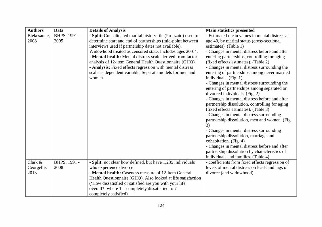
124

Authors Data Details of Analysis Main statistics presented Blekesaune, 2008

BHPS, 1991-2005

- Split: Consolidated marital history file (Pronzato) used to determine start and end of partnerships (mid-point between interviews used if partnership dates not available). Widowhood treated as censored state. Includes ages 20-64. - Mental health: Mental distress scale derived from factor analysis of 12-item General Health Questionnaire (GHQ). - Analysis: Fixed effects regression with mental distress scale as dependent variable. Separate models for men and women.

- Estimated mean values in mental distress at age 40, by marital status (cross-sectional estimates). (Table 1) - Changes in mental distress before and after entering partnerships, controlling for aging (fixed effects estimates). (Table 2) - Changes in mental distress surrounding the entering of partnerships among never married individuals. (Fig. 1) - Changes in mental distress surrounding the entering of partnerships among separated or divorced individuals. (Fig. 2) - Changes in mental distress before and after partnership dissolution, controlling for aging (fixed effects estimates). (Table 3) - Changes in mental distress surrounding partnership dissolution, men and women. (Fig. 3) - Changes in mental distress surrounding partnership dissolution, marriage and cohabitation. (Fig. 4) - Changes in mental distress before and after partnership dissolution by characteristics of individuals and families. (Table 4)

Clark & Georgellis 2013

BHPS, 1991 - 2008

- Split: not clear how defined, but have 1,235 individuals who experience divorce - Mental health: Caseness measure of 12-item General Health Questionnaire (GHQ). Also looked at life satisfaction (‘How dissatisfied or satisfied are you with your life overall?’ where 1 = completely dissatisfied to 7 = completely satisfied)

- coefficients from fixed effects regression of levels of mental distress on leads and lags of divorce (and widowhood).

125

Authors Data Details of Analysis Main statistics presented - Analysis: within-subject (fixed effects) approach to look at four years preceding and five years following. Separate models for men and women. Omitted category is therefore people who are married and not experiencing a divorce .

Aassve and Tavares, 2013

BHPS, 1991 - 2008

- Split: Excluded those who joined sample as a couple if there was no retrospective information available from the marital history file (so they could measure duration of partnership). Final sample is composed of 577 individuals. - Mental health: Mental distress scale derived from factor analysis of 12-item General Health Questionnaire (GHQ). This needed to be observed at two years before and 1 year after the split. - Analysis: regression with change in mental distress between t+1 and t-2 as dependent variable.

- Changes in mental distress before and after end of partnership, by partnership state (Fig 1) - Impact of characteristics on changes in mental distress at end of partnership (measured as (t+1) – (t-2)). - Same model but where outcome is a binary variable for GHQ >= 14 immediately after union dissolution

126

Annex B. Supplementary results B.1 Comparing estimates of median income from BHPS and official HBAI datasets

As the UK BHPS sample includes over-samples of Scottish, Welsh and Northern Irish

residents we also compare with weighted BHPS estimates. As design weights are not

provided, we computed these weights by computing the selection probability as the ratio of

the 2001 regional sample sizes to the UK 2001 Census population for these four regions and

taking its inverse. In the figures below, we plot median AHC and BHC income estimated by

use from the BHPS and the official values of median income from the HBAI series. Our

BHPS-based estimates of BHC income are marginally lower, and our estimates of AHC

incomes are higher (perhaps reflecting that we cannot measure all of the things which HBAI

considers to be a “housing cost”).

127

Figure B1. Comparing median net AHC and BHC equivalised real household income from BHPS (our calculation) and FRS (as reported by IFS) (2009 prices)

250

300

350

400

450

£ pe

r wee

k

1990 1995 2000 2005 2010interview year

median net AHC household income2009 prices, equivalized

250

300

350

400

450

£ pe

r wee

k

1990 1995 2000 2005 2010interview year

median net BHC household income2009 prices, equivalized

BHPS, GB IFS

250

300

350

400

450

£ pe

r wee

k

1990 1995 2000 2005 2010interview year

median net AHC household income2009 prices, equivalized

250

300

350

400

450

£ pe

r wee

k

1990 1995 2000 2005 2010interview year

median net BHC household income2009 prices, equivalized

BHPS, UK IFS

128

250

300

350

400

450

£ pe

r wee

k

1990 1995 2000 2005 2010interview year

median net AHC household income2009 prices, equivalized

250

300

350

400

450

£ pe

r wee

k

1990 1995 2000 2005 2010interview year

median net BHC household income2009 prices, equivalized

BHPS, UK wtd IFS

129

B.3 Variant to Tables 7 and 8 that controls for more factors. The following tables include all separations (not due to death of a partner) in the BHPS. Table B1. Logit estimation of the likelihood of separating by the next wave (GB sample, only OSMs & PSMs, separation does not include death of partner)

All Women Men

Odds Ratio Odds Ratio Odds Ratio

Gender (Omitted: Men) Women 1.09

Whether has at least one dependent child (Omitted: No) Has at least one dependent child 0.73** 0.77* 0.71**

Age of youngest child 1.04** 1.04** 1.03* Age group (Omitted: 30-39 years)

Age 15-19 years 2.84** 2.86** 3.29** Age 20-29 years 1.43** 1.57** 1.28* Age 40-49 years 0.58** 0.56** 0.62** Age 50-59 years 0.32** 0.24** 0.40** Age 60+ years 0.09** 0.07** 0.10**

Current marital status (Omitted: Married) Cohabiting 3.73** 3.52** 3.93**

Interview year (Omitted: 1998 – 2003) 1991 – 1997 1.02 1.01 1.02

2004 – 2008 0.96 1.05 0.87 Highest educational qualifications (Omitted: None)

GCSE or A-levels 1.23* 1.29+ 1.16 Higher 1.05 1.07 1.02

Current employment status (Omitted: Not employed) Currently employed 0.95 1.08 0.80+

Housing Tenure (Omitted: Owned with mortgage) Owned outright 0.82 1.06 0.62*

Renting, Social Housing 1.53** 1.72** 1.31* Renting, Other 1.81** 1.98** 1.64**

Net Current Household BHC income (Omitted: Less than 25th percentile)

25th to 50th percentile 0.86+ 0.84 0.89 50th to 75th percentile 0.76** 0.72** 0.85 75th percentile or higher 0.73** 0.68** 0.78

Constant 0.02** 0.02** 0.03** Number of Observations 68390 33957 34433 + p<0.10, * p<0.05, ** p<.01

130

Table B2. Logit estimation of the likelihood of separating by the next wave (GB sample, only OSMs & PSMs, separation does not include death of partner)

Women with dependent children in

the interview before

separation

Women without

dependent children in the

interview before

separation

Men with dependent children in

the interview

before separation

Men without dependent children in

the interview

before separation

Odds Ratio Odds Ratio Odds Ratio Odds Ratio

Age of youngest child 1.05**

1.00 Age group (Omitted: 30-39 years)

Age 15-19 years 2.76** 2.86** 2.11 4.26** Age 20-29 years 1.73** 1.40* 1.38+ 1.28* Age 40-49 years 0.51** 0.71 0.72+ 0.51** Age 50-59 years 0.35* 0.25** 0.60 0.34** Age 60+ years

0.07** 0.69 0.09**

Current marital status (Omitted: Married)

Cohabiting 3.22** 4.04** 2.92** 4.94**

Interview year (Omitted: 1998 – 2003)

1991 – 1997 0.99 1.08 1.01 1.03 2004 – 2008 1.05 1.09 1.01 0.78

Highest educational qualifications (Omitted: None)

GCSE or A-levels 1.32+ 1.21 1.26 1.03 Higher 1.01 1.09 0.88 1.07

Current employment status (Omitted: Not employed)

Currently employed 1.12 0.96 0.71+ 0.83 Housing Tenure (Omitted: Owned with mortgage)

Owned outright 0.93 1.14 0.99 0.49** Renting, Social Housing 1.81** 1.46* 1.20 1.50* Renting, Other 1.93** 2.02** 1.64+ 1.56**

Net Current Household BHC income (Omitted: Less than 25th percentile)

25th to 50th percentile 0.92 0.64* 0.93 0.92 50th to 75th percentile 0.80 0.59** 0.98 0.81 75th percentile or higher 0.75 0.58* 0.70 0.86

Any biological children

0.86

1.31 Constant 0.01** 0.02** 0.02** 0.03** Number of Observations 15293 18662 14253 20084 + p<0.10, * p<0.05, ** p<.01

131

B.3 Variant to Tables 31 and 32 that control for more factors. We find that higher education individuals are better able to cope with separation.

Employment is beneficial for mental health for all groups except for men with children. For

this group, compared to those who were employed before separation and still are, those were

not employed at both time points, have lower levels of stress. We expected that if it were the

case that at least one child who was living with the person before separation is not living with

them at separation, then that would increase stress. While this is the case for women with

children, the opposite is true for men with children. The omitted category comprises of those

who have custody of all their children. As among men this is a very small percentage, it is

possible that this is a very select group of men and hence the counter intuitive results.

Repartnering has a positive effect on mental health. Marital status before separation does not

matter. To measure any period effects we included a dummy for whether the current

interview year is in 2000-2008. We find that all groups other than men without dependent

children are likely to be happier in the 2000s as compared to the 1990s.

132

Table B3. Estimated coefficients of an OLS regression of the absolute change in GHQ-12 (0-36 scale) measured from 2 interviews prior to separation with additional covariates

Women with dependent

children in the interview before

separation

Women without dependent

children in the interview before

separation

Men with dependent

children in the interview before

separation

Men without dependent

children in the interview before

separation Constant 5.410** 5.418** 6.203** 6.253** 7.097** 7.124** 0.209 0.21 1 year after first observed as single -2.115** -2.120** -2.070** -2.081** -3.953** -3.961** -1.964** -1.971** 2 years after first observed as single -2.689** -2.696** -1.215 -1.238 -4.626** -4.631** -1.897** -1.911** 3 years after first observed as single -2.694** -2.704** -1.358* -1.398* -3.888** -3.885** -1.329* -1.353* 4+ years after first observed as single -3.774** -3.729** -2.172+ -2.154+ -3.713** -3.710** -4.312** -4.326** 4+ years after first observed as single, slope 0.147 0.134 0.136 0.127 0.054 0.054 0.297** 0.292** Proportionate Change in Net Household BHC Income 0.169

-0.261

0.137

-0.153

Proportionate Change in Net Household AHC Income

0.221*

-0.09

0.086

-0.019

Educational qualification at two years before separation: None (Omitted)

A-level/GCSE -2.769** -2.787** -3.838** -3.858** -0.169 -0.178 2.548** 2.542**

Higher degree -4.161** -4.150** -3.474** -3.514** -0.889 -0.89 2.117** 2.103** Age group: 30-39 years (Omitted)

16-29 years -0.894+ -0.903+ 0.952+ 0.922+ 0.104 0.095 -0.266 -0.269

40-49 years -0.598 -0.586 -2.550** -2.522** -0.549 -0.549 -0.349 -0.332

50+ years -2.167** -2.109** -3.909** -3.858** -3.082** -3.086** -1.378** -1.427**

Re-partnered -1.216** -1.285** -1.322** -1.326** -0.339 -0.348 -0.873* -0.901* At least one of the children present at year before separation co-resident right after separation 1.223* 1.249*

-2.711** -2.709**

Number of own children in HH -0.316+ -0.299+ 0.367 0.39 0.153 0.147 0.25 0.288 Employment status at two years prior to separation, current: Employed, Employed (Omitted)

Not employed, Not Employed 1.181** 1.175** 0.079 0.128 -2.212** -2.232** 2.259** 2.258** Not employed, Employed -0.116 -0.197 -0.916 -0.938 -0.981 -1.006 -1.478** -1.569** Employed, Not Employed 1.858** 1.885** 0.048 0.083 4.077** 4.050** 0.042 0.121

Year of separation: 1998 – 2003 (Omitted)

Year 1991 – 1997 -1.705** -1.720** -0.870* -0.906* 1.019* 1.014* 1.004** 0.999**

Year 2004 – 2008 1.257* 1.227* 1.007 0.976 -0.404 -0.446 1.138+ 1.144+ Marital status in the year before separation: Cohabiting (Omitted)

Married 0.585 0.587 1.323** 1.343** -0.549 -0.523 1.180** 1.202** At least one biological child prior to separation

-1.24 -1.292+

-0.298 -0.274

Number of observations 2362 2362 1811 1811 1480 1480 1707 1707

R-squared 0.084 0.085 0.075 0.075 0.113 0.113 0.071 0.07

Note: Year refers to annual interviews

133

We also estimated models where instead of household income we included direct measures of

financial stress and found that greater financial stress is associated with higher levels of

mental distress. However, as subjective measures of health and well-being are generally

found to be correlated, we also estimated a simple model of the association between

household income (AHC and BHC) on likelihood of experiencing financial distress

(dichotomised the 5 category measure of financial distress where the last the categories were

coded as 1). We found that except for women without dependent children, higher incomes

reduce the likelihood of reporting financial stress.

134

Table B4. Estimated coefficients of an OLS regression of the absolute change in GHQ-12 (0-36 scale) measured from 2 interviews prior to separation with a measure of financial stress instead of household income as one of the covariates

Women with dependent children in the interview before

separation

Women with no dependent children in the interview before

separation

Men with dependent children in the interview before

separation

Men with no dependent children in the interview before

separation

Constant 0.69 4.068** 0.523 4.331** 1.310+ 4.630** 1.858** -0.622 1 year after first observed as single -2.189** -2.065** -2.293** -1.924* -3.363** -3.365** -1.954** -1.802** 2 years after first observed as single -2.501** -2.389** -1.486+ -0.987 -3.918** -3.972** -2.067** -1.670** 3 years after first observed as single -2.909** -2.432** -1.925** -1.078 -2.886** -2.824** -1.591** -1.170* 4+ years after first observed as single -3.535** -3.401** -2.516* -1.927 -3.508** -3.209* -3.819** -3.859** 4+ years after first observed as single, slope 0.033 0.142 0.036 0.134 0.134 0.163 0.220* 0.268**

Living comfortably (Omitted) Doing Alright 0.399 0.131 1.208* 0.813+ 0.778 0.732 0.635+ 0.622+

Just about getting by 1.921** 1.191* 1.432** 1.336** 2.167** 2.504** 0.830* 0.867*

Finding it quite difficult 2.900** 2.167** 4.463** 4.794** 5.584** 5.562** 1.819** 1.975**

Finding it very difficult 5.268** 4.416** 7.702** 7.103** 7.021** 7.154** 4.807** 5.579** Educational qualification at two years before separation: None (Omitted)

A-level/GCSE

-2.708**

-3.310**

0.142

2.601**

Higher degree

-4.056**

-2.947**

-0.474

2.244** Age group 30-39 years (Omitted)

16-29 years

-0.771

0.754

0.594

-0.281

40-49 years

-0.438

-2.571**

-0.707

-0.274

50+ years

-2.093**

-3.307**

-2.961**

-1.193*

Partner present

-0.660+

-0.829*

0.01

-0.795* At least one child co-resident in year before separation co-resident right after

1.092*

-3.082**

Number of own children in HH

-0.308+

0.163

0.109

0.183 Employment status at two years before separation, current: Employed, Employed (Omitted)

Not employed, Not Employed

0.816+

-0.881

-3.404**

1.509*

Not employed, Employed

-0.006

-1.384*

-1.926*

-1.817**

Employed, Not Employed

1.220*

-0.549

1.651*

-0.508 Year of separation: 1998 – 2003 (Omitted)

Year 1991 – 1997

-1.647**

-0.920*

0.793*

0.935**

Year 2004 – 2008

1.182+

1.215+

-0.484

0.963 Marital status at separation: Cohabiting (Omitted)

Married

0.54

1.582**

-0.392

1.142** At least one biological children prior to separation

-1.823*

-0.223

Number of observations 2361 2361 1813 1809 1478 1478 1719 1705

R-squared 0.056 0.103 0.052 0.108 0.11 0.096 0.169 0.032 + p<0.10, * p<0.05, ** ,p<.01*** Note: Year refers to annual interviews

135