Embed Size (px)
Citation preview
Passive Inter-modulation Cancellationin FDD System
FAN CHENMASTER´S THESISDEPARTMENT OF ELECTRICAL AND INFORMATION TECHNOLOGY |FACULTY OF ENGINEERING | LTH | LUND UNIVERSITY
Printed by Tryckeriet i E-huset, Lund 2017
FAN
CH
ENPassive Inter-m
odulation Cancellation in FD
D System
LUN
D 2017
Series of Master’s thesesDepartment of Electrical and Information Technology
LU/LTH-EIT 2017-563
http://www.eit.lth.se
Passive Inter-modulation Cancellation in FDD System
Master Thesis in Wireless Communication
Faculty of Engineering, Lund University and Radio System, Ericsson AB, Lund
Fan Chen
March 2017
i
Abstract Passive inter-modulation (PIM) shows up when two or more RF signals are mixed together via the nonlinear passive devices. With the rapid development and expansion of the wireless com-munication networks, PIM is recognized as one of the most critical issues.
Especially in the base station, where several networks systems have to share the same infrastruc-ture, a few transmitted signals are physically close to each other, even they could be sharing the same antenna. So it is highly possible that several transmitted signals hit a same nonlinear junc-tion and generate PIM distortion, then the PIM distortion falls in some bands of the receivers nearby.
Even more critically, since some technologies are developed with multi-carrier or multi-band, such as Carrier Aggregation and MIMO, the generated PIM could spread in a wide range of the spectrum and overlap with the receiver bands.
Additionally the continuous increased power of the transmitted signals and the hyper sensitivity of the received signals make PIM issue particularly critical in the base station. Even the fifth and seventh order products of PIM could cause the performance degradation on the received signals.
Isolation and shielding have been used to suppress the effect of PIM distortion, but it is costly and space-consuming solution. In this thesis, a digital self-adaptive cancellation technique is in-troduced. In the proposed technique, an estimated PIM is created based on the known baseband transmitted signal which is highly correlated to the PIM distortion present in the receiver chain, then the received signal is extracted by subtracting the estimated PIM signal from the distorted received signal in the digital domain.
Time-dependency is one of the natures of PIM, since the nonlinearity of the passive devices al-ways varies with temperature, humidity and elements age. To realize an accurate estimation of PIM distortion in real time, the adaptive filter with NLMS (Normalized Least Mean Square) and RLS (Recursive Least Squares) algorithms is used to adjust the coefficients of the filter in the cancellation block.
To ensure the expected performance of the technique to be reached, many simulations under dif-ferent situations are implemented and analyzed in Matlab. Additionally some proper simplifica-tions in the cancellation block are proceeded so that this technique can be realized in the hard-ware at a low cost in future.

ii
Acknowledgements First of all, I would like to thank Jonas Persson for giving me a challenging topic to work on at Ericsson in Lund.
I am highly grateful to my supervisors Henrik Sjöland from Lund University and Lars Lennarts-son from Ericsson for their guidance and support throughout the whole phase of project. They are always there when I need help.
I would also like to thank Sven Mattisson and Peter Hallberg from Ericsson for the continuous support. Without your help and support, I couldn’t accomplish the project as expected.
Finally I would like to thank all the students in Wireless Communication group who help and en-courage me with my study and work.

iii
Abbreviations FDD Frequency Division Duplex
PIM Passive Inter-modulation
RF Radio Frequency
CA Carrier Aggregation
MIMO Multiple Input Multiple Output
RLS Recursive Least Squares
LMS Least Mean Square
NLMS Normalized Least Mean Square
SPR Signal-PIM-Ratio
LTE Long Term Evolution
BTS Base Transceiver Station
UL Uplink
DL Downlink
DAC Digital-Analogue Conversion
ADC Analogue-Digital Conversion
SS Step Size
FF Forgetting Factor
IIR Infinite Impulse Response
FIR Finite Impulse Response
OSR Oversampling Rate
BPF Band Pass Filter
iv
Contents
1 Introduction ........................................................................................................................... 1
1.1 Background ................................................................................................................. 1
1.2 Tasks and Purposes ..................................................................................................... 1
1.3 Limitations .................................................................................................................. 2
1.4 Thesis Outline ............................................................................................................. 2
2 PIM Distortion ...................................................................................................................... 3
2.1 What is PIM Distortion ............................................................................................... 3
2.2 Causes of PIM Distortion ............................................................................................ 4
2.3 Harm of PIM Distortion .............................................................................................. 4
2.4 Prevention and Suppression of PIM Distortion .......................................................... 5
2.5 PIM Model .................................................................................................................. 6
3 Adaptive Algorithms Theory ................................................................................................ 8
3.1 Principle of Adaptive Filter ......................................................................................... 8
3.2 NLMS (Normalized Least Mean Square) Algorithm ................................................ 10
3.3 Recursive Least Squares Algorithm (RLS) ............................................................... 13
4 Simulation Model Design ................................................................................................... 16
4.1 General Consideration of Simulator .......................................................................... 16
4.2 Simulator Overview .................................................................................................. 17
4.3 Simulator Model Design ........................................................................................... 18
4.3.1 Transmitter ................................................................................................................... 18
4.3.2 PIM Generator ............................................................................................................. 19
v
4.3.3 Receiver ....................................................................................................................... 20
4.3.4 Cancellation Block Design........................................................................................... 21
5 Simulation Result................................................................................................................ 23
5.1 Cancellation of Pure PIM (Scenario 1) ..................................................................... 24
5.1.1 PIM Simulation by diode-like Model .......................................................................... 24
5.1.2 Cancellation of Pure PIM ............................................................................................. 25
5.2 Cancellation of Mixed Signals .................................................................................. 28
5.2.1 Comparison of Algorithm (RLS and NLMS) .............................................................. 28
5.2.2 Different Oversampling Rate ....................................................................................... 31
5.2.3 Different values for the parameter Vt........................................................................... 32
5.2.4 Different SPR_bef ........................................................................................................ 33
5.3 Cancellation in Time-Varying Environment ............................................................. 34
6 Conclusion .......................................................................................................................... 37
Appendix A Taylor Series for exponential function ..................... 39
Appendix B The Structure of LTE FDD Frame ........................... 40
Appendix C More Simulation Results .......................................... 41
References .............................................................................................................................. 46
1
1 Introduction
1.1 Background
PIM is the distortion resulting from the nonlinear mixing of two or more signals with different frequencies via passive devices. With the development of LTE and LTE Advanced networks, the technologies with multi-band and multi-carrier are used very commonly, which makes PIM issue more challenging. For example as one of the key technologies in LTE Advanced system, carrier aggregation (CA) combines the different fragmentary bands to get a wider spectrum. With the aggregation of more and more downlink carriers, PIM distortion generated by those carriers takes up relative wider spectrum resource and the generated PIM product could fall in the uplink bands. When this happens, the UL signal of BTS will degraded significantly.
Even more critical, with the development of the radio frequency communication system, the DL signal power is growing continually higher and meanwhile the UL signal is required to be hyper-sensitive. Any nonlinearity generated by the high-power DL signals could be critical to the sensi-tive UL signals.
Another key factor affecting PIM level is the RF path. With the increase of the passive devices number, such as splitters, transmission line, and connectors, these elements have to be placed closer to the antenna and this situation can contribute to PIM generation. And also the aging of the mechanical elements and devices make PIM issue more critical.
PIM distortion is a weak nonlinearity, but it could distort the UL signal significantly because of the combination of high power of the DL signal and the hypersensitive UL signal. As a conse-quent, PIM can limit the capacity and range of the communication system by interfering with the desired received signal. Isolation and shielding of antenna could reduce the effect of PIM, but it is a very costly and space consuming solution. In this thesis, a more effective and less expensive method is introduced.
1.2 Tasks and Purposes
This thesis aims to develop a self-adaptive method to suppress PIM distortion caused by the DL signals and meanwhile a low oversampling rate of the cancellation circuit should be realized. This method is based on the known baseband transmitted signal of the transceiver system and it is implemented in the digital domain.
In this thesis, a self-adaptive method with two different algorithms is developed to suppress PIM distortion in the digital domain. A quick convergence rate and a good stable state are both re-quired under different situations and considering the environment variation such as temperature and mechanical force, the tracking capability is examined and analyzed by different designing parameters. In this proposed method, NLMS and RLS adaptive algorithms are separately applied
2
to update the coefficients of the FIR adaptive filter and the properties of these two algorithms are compared with the simulation results. As a result, one of these algorithms is chosen to continue the further study. The main tasks in this thesis involve,
The mechanism of PIM distortion is studied and some general defensive measures are in-troduced.
A nonlinear model – diode-like model is introduced to represent PIM distortion. The basic theorem of the adaptive filter is studied. NLMS and RLS algorithms are intro-
duced and compared. The cancellation block with a low oversampling rate is designed to eliminate the PIM dis-
tortion in the digital domain. Only PIM distortion is present in the receiver chain with the absence of received signal.
The diode-like model is studied via some simulations in this scenario. The validity of the simulator and the cancellation circuit is verified.
For more realistic, the received signal is added to the receiver chain, mixed with PIM dis-tortion. In this scenario, the distortion suppression effect and the convergence rate of LMS and RLS algorithms are analyzed and compared with many simulations under dif-ferent situations. As a comparing result, RLS algorithm is chosen to continue the further study, because of the better performance.
Time-varying PIM distortion caused by the variations of the environment and the trans-mitted signal is considered. To track the distortion variation promptly, different forgetting factors of RLS algorithm is evaluated. A tradeoff is made between the tracking capability and the suppression effect by the forgetting factor.
1.3 Limitations
Although the research has reached the aims, there are some limitations and shortcomings.
The only imperfection of the simulator is PIM distortion Only the 3rd and 5th order of PIM distortion is considered in the cancellation The simulation result is not proved in hardware due to short of time
1.4 Thesis Outline
In Chapter 2, PIM mechanisms is introduced including the causes and harms. Then different sup-pression methods are analyzed and compared. At last an accurate mathematical model of PIM is introduced and it will be used in the simulation. As the key part of the cancellation block, adap-tive filter and its algorithms are introduced in Chapter 3. And also the properties and implemen-tation of LMS and RLS algorithms are described in this chapter. Chapter 4 describes the simula-tion model structure and analyzes the cancellation block model design. Chapter 5 presents the simulation results and compares the performance of different adaptive algorithms in the applica-tion. Chapter 6 makes the conclusion for the simulation results.
3
2 PIM Distortion
Passive Inter-modulation (PIM) has been considered as one of the critical issues in the cellular network. It is very difficult to estimate the generated PIM distortion and cancel it, because PIM is not only related to the source signal but also the RF path, which changes very often by the temperature, humidity or the elements aging and so on.
To prevent and suppress PIM distortion, it’s necessary to study some basic knowledge of PIM distortion. In this chapter, the mechanism of PIM generation and an accurate PIM models will be introduced. Also the PIM suppression will be discussed briefly for a fur-ther study.
2.1 What is PIM Distortion
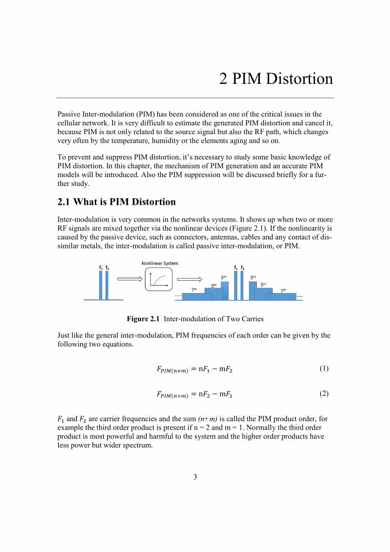
Inter-modulation is very common in the networks systems. It shows up when two or more RF signals are mixed together via the nonlinear devices (Figure 2.1). If the nonlinearity is caused by the passive device, such as connectors, antennas, cables and any contact of dis-similar metals, the inter-modulation is called passive inter-modulation, or PIM.
Figure 2.1 Inter-modulation of Two Carries
Just like the general inter-modulation, PIM frequencies of each order can be given by the following two equations.
( ) = n − m (1)
( ) = n − m (2)
and are carrier frequencies and the sum (n+m) is called the PIM product order, for example the third order product is present if n = 2 and m = 1. Normally the third order product is most powerful and harmful to the system and the higher order products have less power but wider spectrum.
4
Another important nature of PIM is time-dependency, since the mechanical devices al-ways vary with the temperature, humidity and elements age etc. In other words, PIM is time-varying distortion.
2.2 Causes of PIM Distortion
Any non-linear junctions could be the cause to generate PIM distortion due to the non-linear current-voltage behavior. Some common reasons are listed as below,
Metal-metal contact surfaces separated by a thin oxide will exhibit MIM diode conduction
rough contact surfaces of metal-metal will cause current crowding at spots where conduction is both resistive and capacitive
Non-linear materials
And the state of all these reasons depends on the environment conditions, such as the temperature, humility, mechanical force and elements age, which means PIM distortion is a time-dependency distortion and has to be detected and eliminated online. Even on the same surface, the repeated measurement could show big difference.
2.3 Harm of PIM Distortion
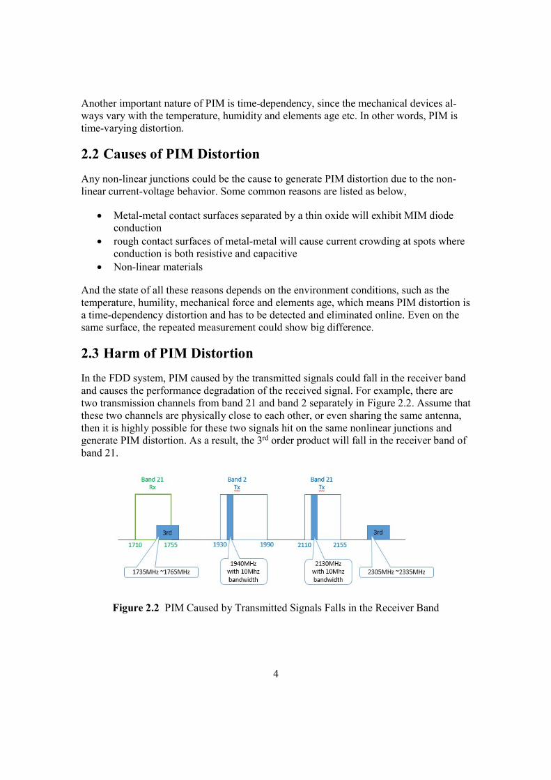
In the FDD system, PIM caused by the transmitted signals could fall in the receiver band and causes the performance degradation of the received signal. For example, there are two transmission channels from band 21 and band 2 separately in Figure 2.2. Assume that these two channels are physically close to each other, or even sharing the same antenna, then it is highly possible for these two signals hit on the same nonlinear junctions and generate PIM distortion. As a result, the 3rd order product will fall in the receiver band of band 21.
Figure 2.2 PIM Caused by Transmitted Signals Falls in the Receiver Band
5
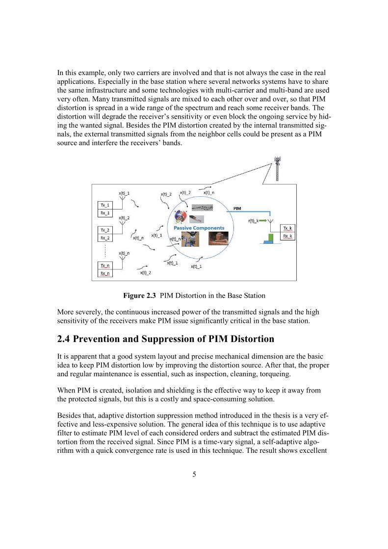
In this example, only two carriers are involved and that is not always the case in the real applications. Especially in the base station where several networks systems have to share the same infrastructure and some technologies with multi-carrier and multi-band are used very often. Many transmitted signals are mixed to each other over and over, so that PIM distortion is spread in a wide range of the spectrum and reach some receiver bands. The distortion will degrade the receiver’s sensitivity or even block the ongoing service by hid-ing the wanted signal. Besides the PIM distortion created by the internal transmitted sig-nals, the external transmitted signals from the neighbor cells could be present as a PIM source and interfere the receivers’ bands.
Figure 2.3 PIM Distortion in the Base Station
More severely, the continuous increased power of the transmitted signals and the high sensitivity of the receivers make PIM issue significantly critical in the base station.
2.4 Prevention and Suppression of PIM Distortion
It is apparent that a good system layout and precise mechanical dimension are the basic idea to keep PIM distortion low by improving the distortion source. After that, the proper and regular maintenance is essential, such as inspection, cleaning, torqueing.
When PIM is created, isolation and shielding is the effective way to keep it away from the protected signals, but this is a costly and space-consuming solution.
Besides that, adaptive distortion suppression method introduced in the thesis is a very ef-fective and less-expensive solution. The general idea of this technique is to use adaptive filter to estimate PIM level of each considered orders and subtract the estimated PIM dis-tortion from the received signal. Since PIM is a time-vary signal, a self-adaptive algo-rithm with a quick convergence rate is used in this technique. The result shows excellent
6
suppression properties with a low cost. The following chapters will describe and evaluate this method with matlab simulations.
2.5 PIM Model
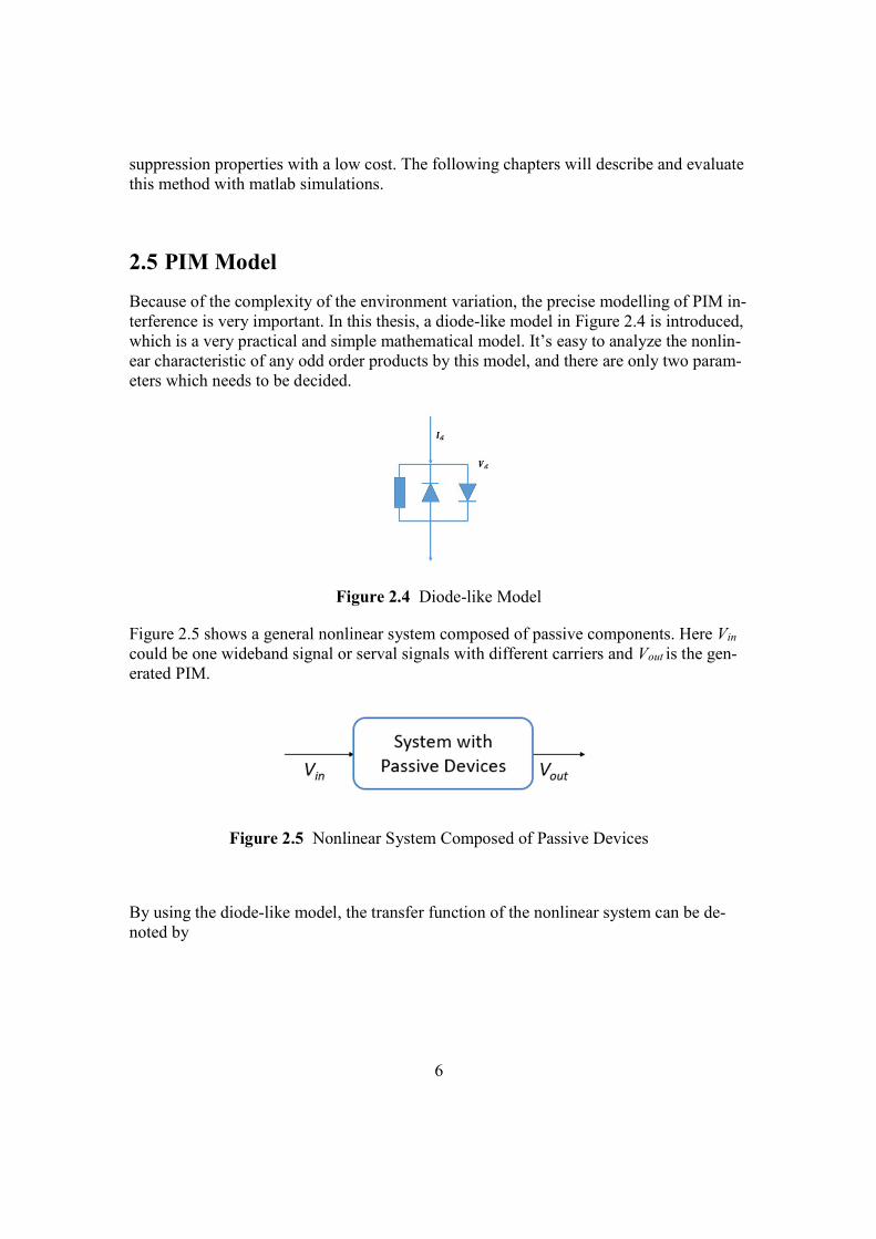
Because of the complexity of the environment variation, the precise modelling of PIM in-terference is very important. In this thesis, a diode-like model in Figure 2.4 is introduced, which is a very practical and simple mathematical model. It’s easy to analyze the nonlin-ear characteristic of any odd order products by this model, and there are only two param-eters which needs to be decided.
Figure 2.4 Diode-like Model
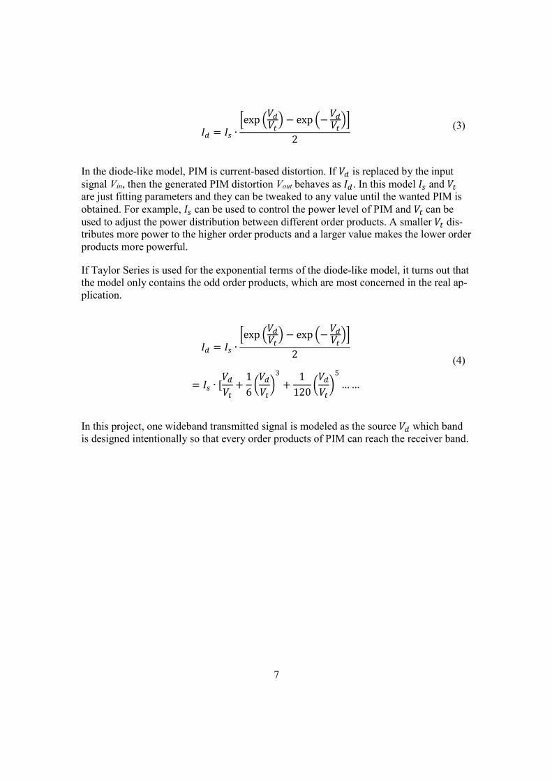
Figure 2.5 shows a general nonlinear system composed of passive components. Here Vin could be one wideband signal or serval signals with different carriers and Vout
is the gen-erated PIM.
Figure 2.5 Nonlinear System Composed of Passive Devices
By using the diode-like model, the transfer function of the nonlinear system can be de-noted by
7
= ∙
exp − exp −
2
(3)
In the diode-like model, PIM is current-based distortion. If is replaced by the input signal Vin, then the generated PIM distortion Vout behaves as . In this model and are just fitting parameters and they can be tweaked to any value until the wanted PIM is obtained. For example, can be used to control the power level of PIM and can be used to adjust the power distribution between different order products. A smaller dis-tributes more power to the higher order products and a larger value makes the lower order products more powerful.
If Taylor Series is used for the exponential terms of the diode-like model, it turns out that the model only contains the odd order products, which are most concerned in the real ap-plication.
= ∙
exp − exp −
2
= ∙ [ +16
+1
120… …
(4)
In this project, one wideband transmitted signal is modeled as the source which band is designed intentionally so that every order products of PIM can reach the receiver band.
8
3 Adaptive Algorithms Theory
One of the most important applications of the adaptive filter is the interference cancellation. Through the parameters self-adaptation by some algorithm, adaptive filter can cancel the inter-ference which spectrum varies over time or overlaps with that of the wanted signals. Moreover adaptive filter can realize the real time tracking task.
As the key part of the adaptive filter, adaptive algorithm is of greatest importance for the conver-gence rate and the stable-state of the filter. RLS and NLMS are two of the most popular algo-rithms because of their own characteristics and advantages. In this project, these two algorithms will be used and evaluated to suppress PIM distortion in the FDD transceiver system.
3.1 Principle of Adaptive Filter
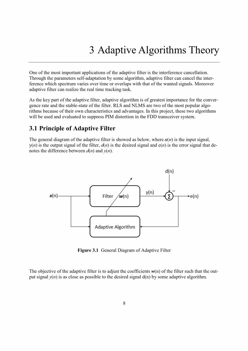
The general diagram of the adaptive filter is showed as below, where x(n) is the input signal, y(n) is the output signal of the filter, d(n) is the desired signal and e(n) is the error signal that de-notes the difference between d(n) and y(n).
The objective of the adaptive filter is to adjust the coefficients w(n) of the filter such that the out-put signal y(n) is as close as possible to the desired signal d(n) by some adaptive algorithm.
Figure 3.1 General Diagram of Adaptive Filter
9
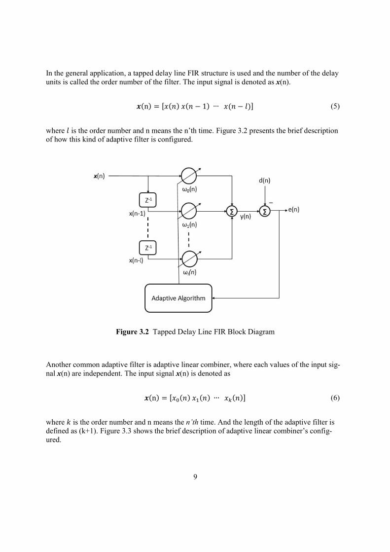
In the general application, a tapped delay line FIR structure is used and the number of the delay units is called the order number of the filter. The input signal is denoted as x(n).
(n) = [ ( ) ( − 1) ∙∙∙ ( − ) (5)
where is the order number and n means the n’th time. Figure 3.2 presents the brief description of how this kind of adaptive filter is configured.
Another common adaptive filter is adaptive linear combiner, where each values of the input sig-nal x(n) are independent. The input signal x(n) is denoted as
(n) = [ ( ) ( ) ∙∙∙ ( ) (6)
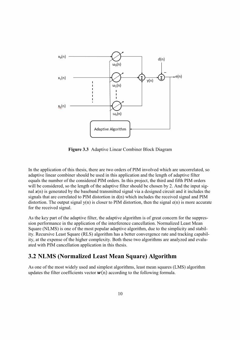
where is the order number and n means the n’th time. And the length of the adaptive filter is defined as (k+1). Figure 3.3 shows the brief description of adaptive linear combiner’s config-ured.
Figure 3.2 Tapped Delay Line FIR Block Diagram
10
In the application of this thesis, there are two orders of PIM involved which are uncorrelated, so adaptive linear combiner should be used in this application and the length of adaptive filter equals the number of the considered PIM orders. In this project, the third and fifth PIM orders will be considered, so the length of the adaptive filter should be chosen by 2. And the input sig-nal x(n) is generated by the baseband transmitted signal via a designed circuit and it includes the signals that are correlated to PIM distortion in d(n) which includes the received signal and PIM distortion. The output signal y(n) is closer to PIM distortion, then the signal e(n) is more accurate for the received signal.
As the key part of the adaptive filter, the adaptive algorithm is of great concern for the suppres-sion performance in the application of the interference cancellation. Normalized Least Mean Square (NLMS) is one of the most popular adaptive algorithm, due to the simplicity and stabil-ity. Recursive Least Square (RLS) algorithm has a better convergence rate and tracking capabil-ity, at the expense of the higher complexity. Both these two algorithms are analyzed and evalu-ated with PIM cancellation application in this thesis.
3.2 NLMS (Normalized Least Mean Square) Algorithm
As one of the most widely used and simplest algorithms, least mean squares (LMS) algorithm updates the filter coefficients vector (n) according to the following formula.
Figure 3.3 Adaptive Linear Combiner Block Diagram
11
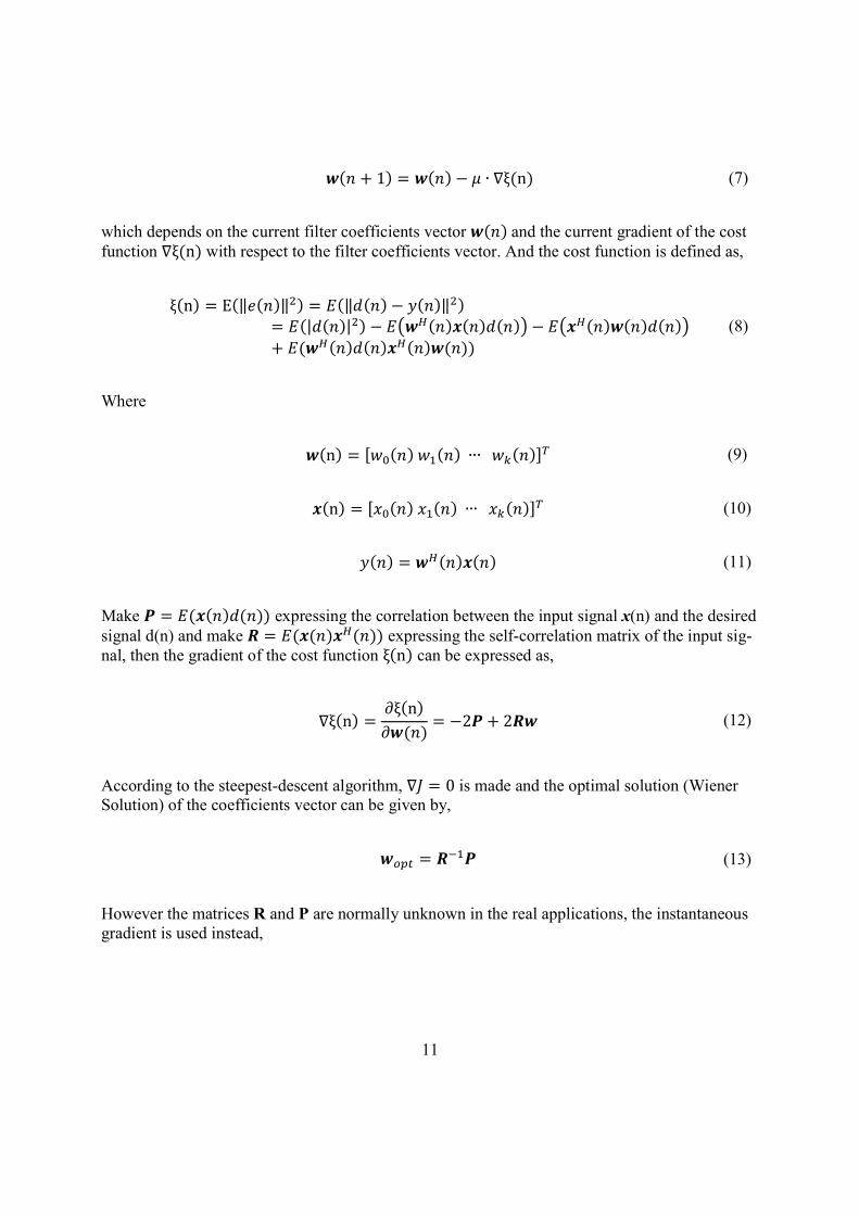
( + 1) = ( ) − ∙ ∇ξ(n) (7)
which depends on the current filter coefficients vector ( ) and the current gradient of the cost function ∇ξ(n) with respect to the filter coefficients vector. And the cost function is defined as,
ξ(n) = E(‖ ( )‖ ) = (‖ ( ) − ( )‖ )
= (| ( )| ) − ( ) ( ) ( ) − ( ) ( ) ( )+ ( ( ) ( ) ( ) ( ))
(8)
Where
(n) = [ ( ) ( ) ∙∙∙ ( ) (9)
(n) = [ ( ) ( ) ∙∙∙ ( ) (10)
( ) = ( ) ( ) (11)
Make = ( ( ) ( )) expressing the correlation between the input signal x(n) and the desired signal d(n) and make = ( ( ) ( )) expressing the self-correlation matrix of the input sig-nal, then the gradient of the cost function ξ(n) can be expressed as,
∇ξ(n) =ξ(n)
( )= −2 + 2 (12)
According to the steepest-descent algorithm, ∇ = 0 is made and the optimal solution (Wiener Solution) of the coefficients vector can be given by,
= (13)
However the matrices R and P are normally unknown in the real applications, the instantaneous gradient is used instead,
12
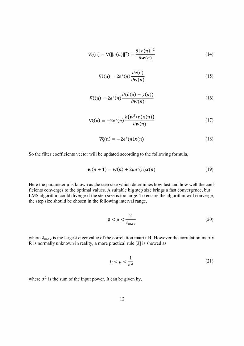
∇ξ(n) = ∇(‖ ( )‖ ) =‖ ( )‖
( ) (14)
∇ξ(n) = 2 ∗( )e(n)
( ) (15)
∇ξ(n) = 2 ∗( )(d(n) − ( ))
( ) (16)
∇ξ(n) = −2 ∗( )(n) ( )
( ) (17)
∇ξ(n) = −2 ∗( ) ( ) (18)
So the filter coefficients vector will be updated according to the following formula,
( + 1) = ( ) + 2 ∗( ) ( ) (19)
Here the parameter μ is known as the step size which determines how fast and how well the coef-ficients converges to the optimal values. A suitable big step size brings a fast convergence, but LMS algorithm could diverge if the step size is too large. To ensure the algorithm will converge, the step size should be chosen in the following interval range,
0 < <2
(20)
where is the largest eigenvalue of the correlation matrix R. However the correlation matrix R is normally unknown in reality, a more practical rule [3] is showed as
0 < <1
(21)
where is the sum of the input power. It can be given by,
13
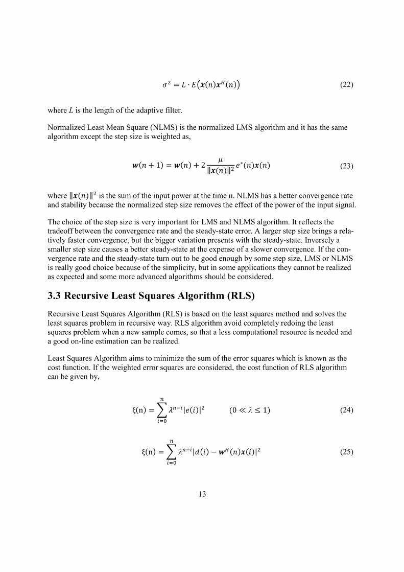
= ∙ ( ) ( ) (22)
where L is the length of the adaptive filter.
Normalized Least Mean Square (NLMS) is the normalized LMS algorithm and it has the same algorithm except the step size is weighted as,
( + 1) = ( ) + 2‖ ( )‖
∗( ) ( ) (23)
where ‖ ( )‖ is the sum of the input power at the time n. NLMS has a better convergence rate and stability because the normalized step size removes the effect of the power of the input signal.
The choice of the step size is very important for LMS and NLMS algorithm. It reflects the tradeoff between the convergence rate and the steady-state error. A larger step size brings a rela-tively faster convergence, but the bigger variation presents with the steady-state. Inversely a smaller step size causes a better steady-state at the expense of a slower convergence. If the con-vergence rate and the steady-state turn out to be good enough by some step size, LMS or NLMS is really good choice because of the simplicity, but in some applications they cannot be realized as expected and some more advanced algorithms should be considered.
3.3 Recursive Least Squares Algorithm (RLS)
Recursive Least Squares Algorithm (RLS) is based on the least squares method and solves the least squares problem in recursive way. RLS algorithm avoid completely redoing the least squares problem when a new sample comes, so that a less computational resource is needed and a good on-line estimation can be realized.
Least Squares Algorithm aims to minimize the sum of the error squares which is known as the cost function. If the weighted error squares are considered, the cost function of RLS algorithm can be given by,
ξ(n) = | ( )| (0 ≪ ≤ 1) (24)
ξ(n) = | ( ) − ( ) ( )| (25)
14
The parameter λ is called forgetting factor which is an exponential weighting factor in the inter-val between 0 and 1. A small forgetting factor reduces the influence of old samples and increases the weight of the new samples, as a result a better tracking capability can be realized at the cost of a higher variance of the filter coefficients. Inversely a large forgetting factor keeps more infor-mation of the old samples and has a lower variance of the filter coefficients, but it takes a longer time to converge when the environment is changed. In the time-varying environment, a tradeoff between the tracking capability and stability has to be made.
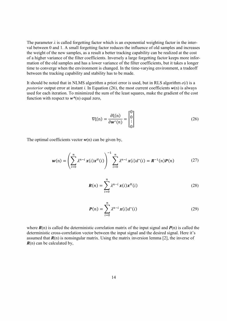
It should be noted that in NLMS algorithm a priori error is used, but in RLS algorithm e(i) is a posterior output error at instant i. In Equation (26), the most current coefficients w(n) is always used for each iteration. To minimized the sum of the least squares, make the gradient of the cost function with respect to w*(n) equal zero,
∇ξ(n) =ξ(n)
∗( )=
00⋮0
(26)
The optimal coefficients vector w(n) can be given by,
(n) = ( ) ( ) ( ) ∗( ) = ( ) ( ) (27)
( ) = ( ) ( ) (28)
( ) = ( ) ∗( ) (29)
where R(n) is called the deterministic correlation matrix of the input signal and P(n) is called the deterministic cross-correlation vector between the input signal and the desired signal. Here it’s assumed that R(n) is nonsingular matrix. Using the matrix inversion lemma [2], the inverse of R(n) can be calculated by,

15
(n) = ( ) =1
( − 1) −( − 1) ( ) ( ) ( − 1)
+ ( ) ( − 1) ( ) (30)
Then the new coefficients w(n) can be updated by,
(n) = (n − 1) + ∗( ) ( ) ( ) (31)
The complex RLS algorithm can be implemented by,
1) Initialization
_ = a (a can be the inverse of the estimation of the input power)
_ = [0 0 … 0 0
2) Iterations e(n) = d(n) − ( − 1) ( ) G = ( − 1) ( )
(n) =1
( − 1) −+
( ) = ( − 1) + ∗( ) ( ) ( )
(The above derivation is introduced very detailed in Adaptive Filtering by Paulo Sergio Ramirez. Please refer to [1] for a better understanding of RLS algorithm.)
RLS algorithm is very good choice for the time-varying environment, because it has a great con-vergence rate and tracking capability. As the cost, RLS has more computational complexity than LMS because of the matrix operations.
16
4 Simulation Model Design
This chapter will introduce the simulator used in Matlab. The simulator composes of transmitter, receiver, PIM generator and cancellation block. The main idea of the simulator design is to make the model as simple as possible under the premise that the interference phenomena can be pre-sented correctly and the cancellation method can be implemented in hardware. To design the model of the cancellation block, the derivation of the input signal of the adaptive filter will be made in this chapter. Meanwhile the spectrums at each stage of the system will be analyzed for a better understanding on PIM distortion.
4.1 General Consideration of Simulator
Too many imperfections involved is not good to study PIM properties and the cancellation be-haviors, so a simplified transceiver model is created in the simulation. It is important to state some assumptions and complexity reductions before getting a deep look into the simulator de-sign. It should be mentioned that the simplification and assumptions will not affect the study of the main points.
Assumptions and complexity reductions
Only imperfection involved in the simulator is PIM distortion. A wide band transmitted signal is used for the input of the PIM generator instead of the
multiple signals. The transmitter and receiver bands are intentionally assigned, so that PIM generated by
transmitted signals can reach the receiver band. Only receiver BPF (Band Pass Filter) is involved in the duplexer. DAC (Digital-Analog Convertor) is replaced by a specific oversampling rate.
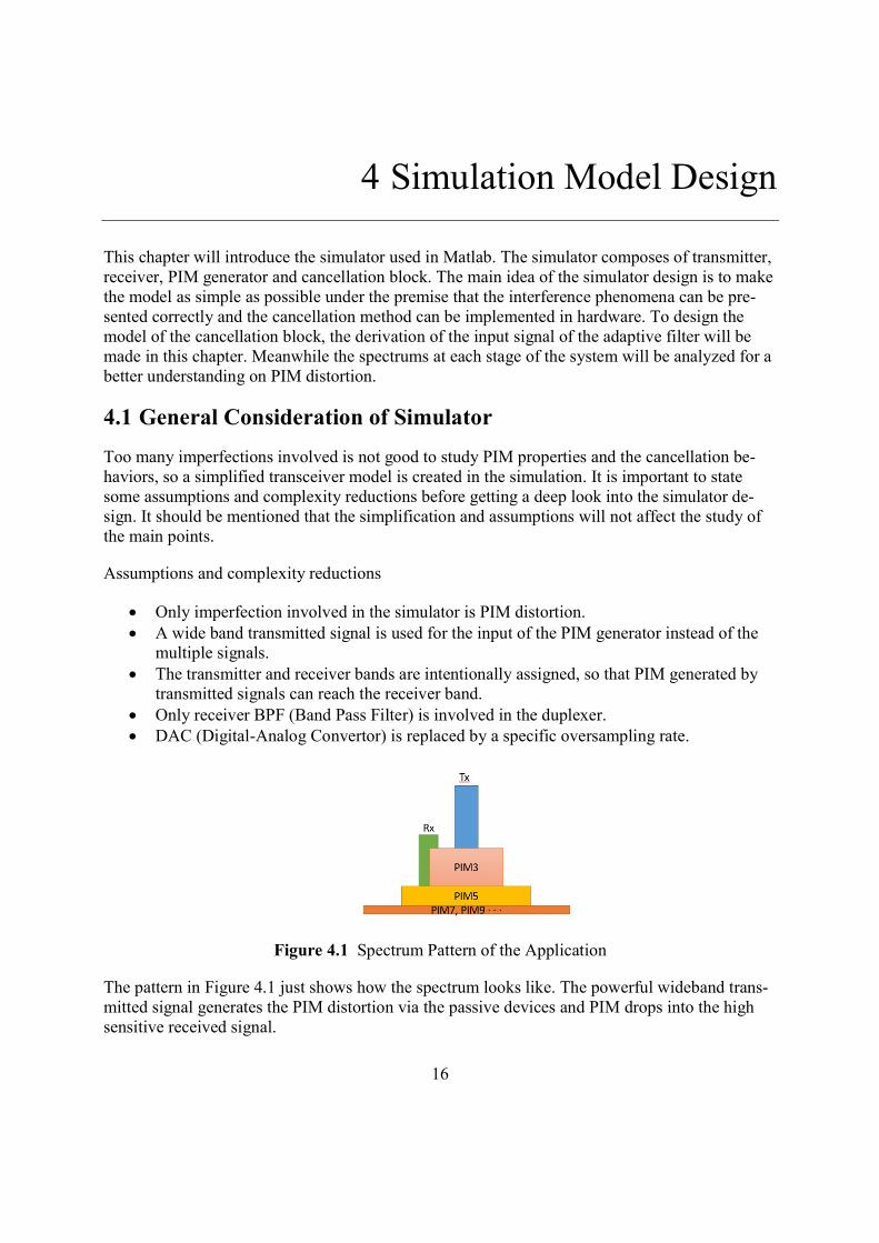
Figure 4.1 Spectrum Pattern of the Application
The pattern in Figure 4.1 just shows how the spectrum looks like. The powerful wideband trans-mitted signal generates the PIM distortion via the passive devices and PIM drops into the high sensitive received signal.
17
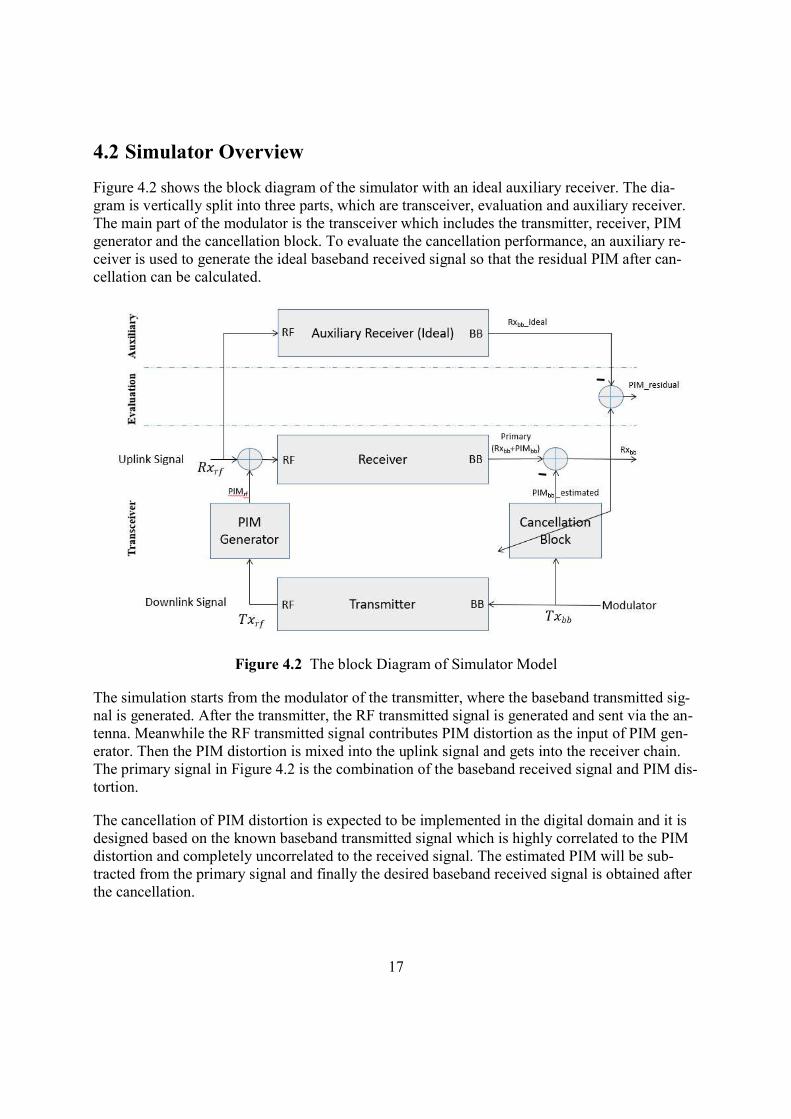
4.2 Simulator Overview
Figure 4.2 shows the block diagram of the simulator with an ideal auxiliary receiver. The dia-gram is vertically split into three parts, which are transceiver, evaluation and auxiliary receiver. The main part of the modulator is the transceiver which includes the transmitter, receiver, PIM generator and the cancellation block. To evaluate the cancellation performance, an auxiliary re-ceiver is used to generate the ideal baseband received signal so that the residual PIM after can-cellation can be calculated.
Figure 4.2 The block Diagram of Simulator Model
The simulation starts from the modulator of the transmitter, where the baseband transmitted sig-nal is generated. After the transmitter, the RF transmitted signal is generated and sent via the an-tenna. Meanwhile the RF transmitted signal contributes PIM distortion as the input of PIM gen-erator. Then the PIM distortion is mixed into the uplink signal and gets into the receiver chain. The primary signal in Figure 4.2 is the combination of the baseband received signal and PIM dis-tortion.
The cancellation of PIM distortion is expected to be implemented in the digital domain and it is designed based on the known baseband transmitted signal which is highly correlated to the PIM distortion and completely uncorrelated to the received signal. The estimated PIM will be sub-tracted from the primary signal and finally the desired baseband received signal is obtained after the cancellation.
18
In the evaluation part, the residual PIM distortion can be obtained by subtracting the ideal re-ceived signal (Rxbb_ideal) from the PIM-suppressed received signal (Rxbb), so that the PIM sup-pression effect by the cancellation block can be analyzed and evaluated.
4.3 Simulator Model Design
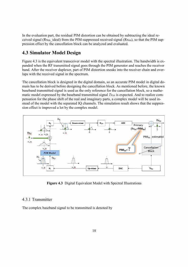
Figure 4.3 is the equivalent transceiver model with the spectral illustration. The bandwidth is ex-panded when the RF transmitted signal goes through the PIM generator and reaches the receiver band. After the receiver duplexer, part of PIM distortion sneaks into the receiver chain and over-laps with the received signal in the spectrum.
The cancellation block is designed in the digital domain, so an accurate PIM model in digital do-main has to be derived before designing the cancellation block. As mentioned before, the known baseband transmitted signal is used as the only reference for the cancellation block, so a mathe-matic model expressed by the baseband transmitted signal Txbb is expected. And to realize com-pensation for the phase shift of the real and imaginary parts, a complex model will be used in-stead of the model with the separated IQ channels. The simulation result shows that the suppres-sion effect is improved a lot by the complex model.
Figure 4.3 Digital Equivalent Model with Spectral Illustrations
4.3.1 Transmitter
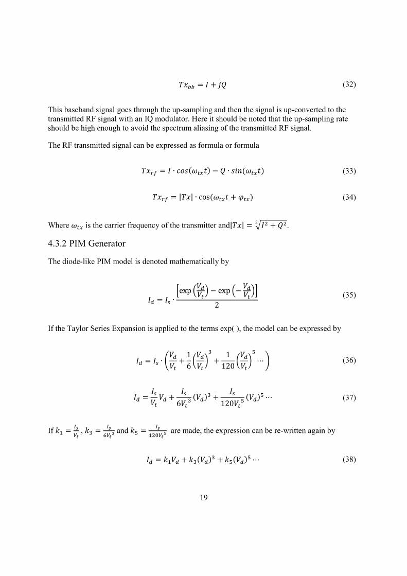
The complex baseband signal to be transmitted is denoted by
19
= + (32)
This baseband signal goes through the up-sampling and then the signal is up-converted to the transmitted RF signal with an IQ modulator. Here it should be noted that the up-sampling rate should be high enough to avoid the spectrum aliasing of the transmitted RF signal.
The RF transmitted signal can be expressed as formula or formula
= ∙ ( ) − ∙ ( ) (33)
= | | ∙ cos ( + ) (34)
Where is the carrier frequency of the transmitter and| | = + .
4.3.2 PIM Generator
The diode-like PIM model is denoted mathematically by
= ∙
exp − exp −
2
(35)
If the Taylor Series Expansion is applied to the terms exp( ), the model can be expressed by
= ∙ +16
+1
120⋯ (36)
= +6
( ) +120
( ) ⋯ (37)
If = , = and = are made, the expression can be re-written again by
= + ( ) + ( ) ⋯ (38)
20
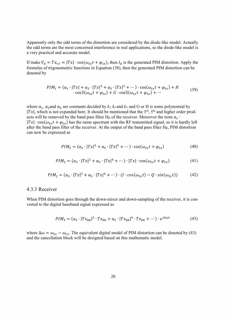
Apparently only the odd terms of the distortion are considered by the diode-like model. Actually the odd terms are the most concerned interference in real applications, so the diode-like model is a very practical and accurate model.
If make = = | | ∙ cos ( + ), then is the generated PIM distortion. Apply the formulas of trigonometric functions in Equation (38), then the generated PIM distortion can be denoted by
= ( ∙ | | + ∙ | | + ∙ | | + ⋯ ) ∙ cos( + ) +∙ cos3( + ) + ∙ cos5( + ) + ⋯
(39)
where , and are constants decided by k1, k3 and k5, and G or H is some polynomial by | |, which is not expanded here. It should be mentioned that the 3rd, 5th and higher order prod-ucts will be removed by the band pass filter HR of the receiver. Moreover the term ∙| | ∙ cos( + ) has the same spectrum with the RF transmitted signal, so it is hardly left after the band pass filter of the receiver. At the output of the band pass filter HR, PIM distortion can now be expressed as
= ( ∙ | | + ∙ | | + ⋯ ) ∙ cos( + ) (40)
= ( ∙ | | + ∙ | | + ⋯ ) ∙ | | ∙ cos( + ) (41)
= ( ∙ | | + ∙ | | + ⋯ ) ∙ ( ∙ ( ) − ∙ ( )) (42)
4.3.3 Receiver
When PIM distortion goes through the down-mixer and down-sampling of the receiver, it is con-verted to the digital baseband signal expressed as
= ( ∙ | | ∙ + ∙ | | ∙ + ⋯ ) ∙ ∆ (43)
where ∆ = − . The equivalent digital model of PIM distortion can be denoted by (43) and the cancellation block will be designed based on this mathematic model.
21
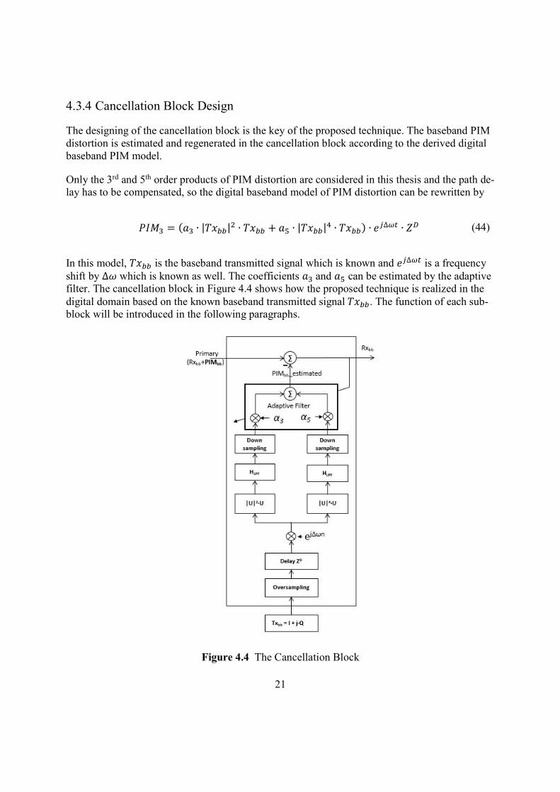
4.3.4 Cancellation Block Design
The designing of the cancellation block is the key of the proposed technique. The baseband PIM distortion is estimated and regenerated in the cancellation block according to the derived digital baseband PIM model.
Only the 3rd and 5th order products of PIM distortion are considered in this thesis and the path de-lay has to be compensated, so the digital baseband model of PIM distortion can be rewritten by
= ( ∙ | | ∙ + ∙ | | ∙ ) ∙ ∆ ∙ (44)
In this model, is the baseband transmitted signal which is known and ∆ is a frequency shift by ∆ which is known as well. The coefficients and can be estimated by the adaptive filter. The cancellation block in Figure 4.4 shows how the proposed technique is realized in the digital domain based on the known baseband transmitted signal . The function of each sub-block will be introduced in the following paragraphs.
Figure 4.4 The Cancellation Block

22
Firstly an oversampling is made at the beginning of the cancellation block to avoid the spectrum aliasing. In this technique, the 3rd and 5th order products of PIM are considered, so the spectrum aliasing will happen without oversampling. Meanwhile a lower oversampling rate (OSR) is rec-ommended, because a higher OSR consumes more on the hardware. Therefore an appropriate OSR is required here. To learn how the OSR affects the cancellation performance, the simulation with different OSR will be studied in Chapter 5.
The second sub-block is delay compensation. It should be mentioned that the duplexer filters of the transceiver is most dominating for the path delay because of the wide bandwidth. Normally IIR filter is used as the duplexer filters, which means the group delay of the duplexer filter is var-iable with the frequency due to the nonlinear phase. This sub-block only compensate for the mean path delay which can be measured offline. And it is assumed that adaptive filter will take care of the variation of the group delay.
Then frequency shift and low pass filter are added separately in the third and fifth sub-blocks. The cancellation block has the same low pass filter with that of the receiver. PIM profiles of the 3rd and 5th order are present in the fourth sub-block.
At last the most important module adaptive filter is applied. In this application, adaptive filter re-alizes three primary functions, which are coefficients estimation, compensation for the phase dis-tortion and PIM tracking in a real-time. For the adaptive filter, the algorithm is the key part. In this application, recursive least squares (RLS) and normalized least square (NLMS) will be eval-uated and compared.
23
5 Simulation Result
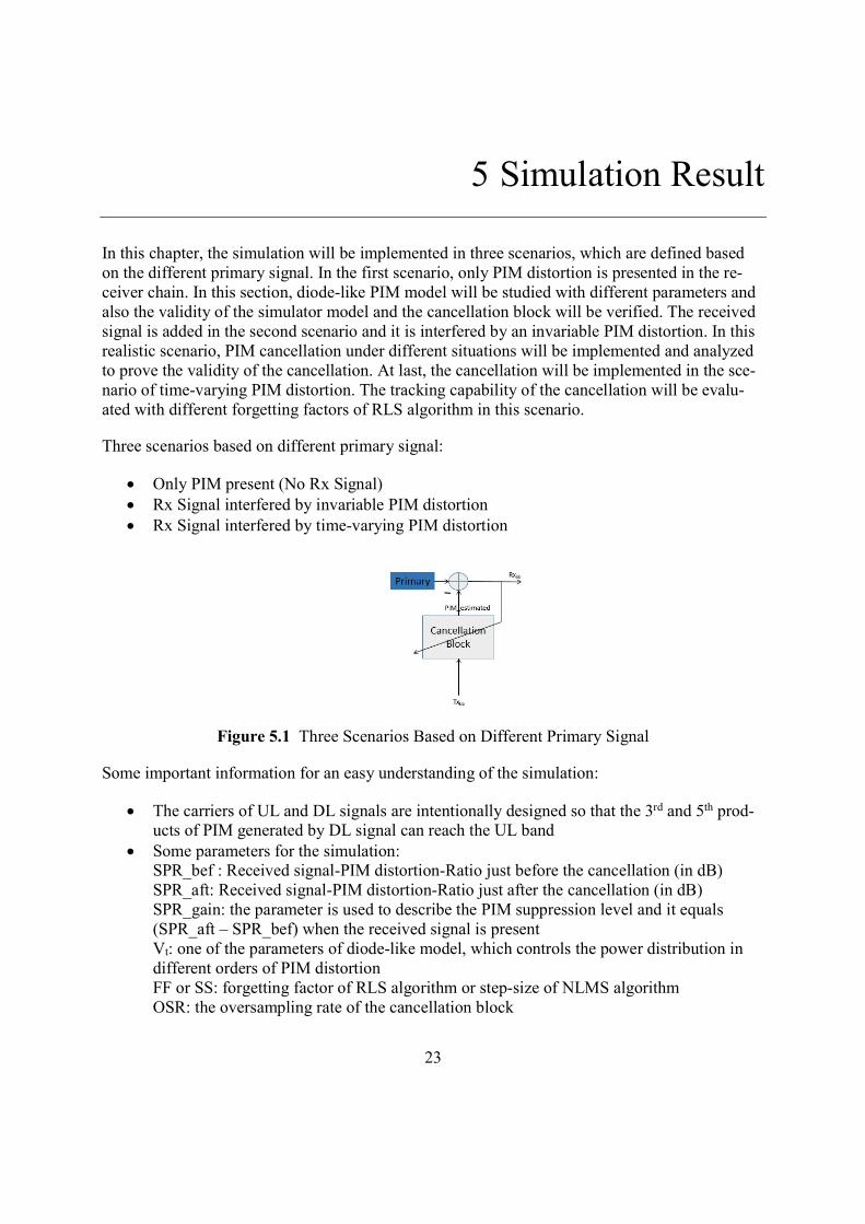
In this chapter, the simulation will be implemented in three scenarios, which are defined based on the different primary signal. In the first scenario, only PIM distortion is presented in the re-ceiver chain. In this section, diode-like PIM model will be studied with different parameters and also the validity of the simulator model and the cancellation block will be verified. The received signal is added in the second scenario and it is interfered by an invariable PIM distortion. In this realistic scenario, PIM cancellation under different situations will be implemented and analyzed to prove the validity of the cancellation. At last, the cancellation will be implemented in the sce-nario of time-varying PIM distortion. The tracking capability of the cancellation will be evalu-ated with different forgetting factors of RLS algorithm in this scenario.
Three scenarios based on different primary signal:
Only PIM present (No Rx Signal) Rx Signal interfered by invariable PIM distortion Rx Signal interfered by time-varying PIM distortion
Figure 5.1 Three Scenarios Based on Different Primary Signal
Some important information for an easy understanding of the simulation:
The carriers of UL and DL signals are intentionally designed so that the 3rd and 5th prod-ucts of PIM generated by DL signal can reach the UL band
Some parameters for the simulation: SPR_bef : Received signal-PIM distortion-Ratio just before the cancellation (in dB) SPR_aft: Received signal-PIM distortion-Ratio just after the cancellation (in dB) SPR_gain: the parameter is used to describe the PIM suppression level and it equals (SPR_aft – SPR_bef) when the received signal is present Vt: one of the parameters of diode-like model, which controls the power distribution in different orders of PIM distortion FF or SS: forgetting factor of RLS algorithm or step-size of NLMS algorithm OSR: the oversampling rate of the cancellation block
24
The power of the received signal keeps same under different conditions A default state is defined by SPR_bef = 15, Vt = 1 and OSR = 4; when evaluating the in-
fluence by changing some specific parameter, the other parameters will keep the default values except the specific one
The coefficients curves of the adaptive filter are used to evaluate the stability and the convergence rate of the algorithm
Only fixed FF or SS is considered, since the aim of this thesis is to solve the problem by finding a solution as simple as possible
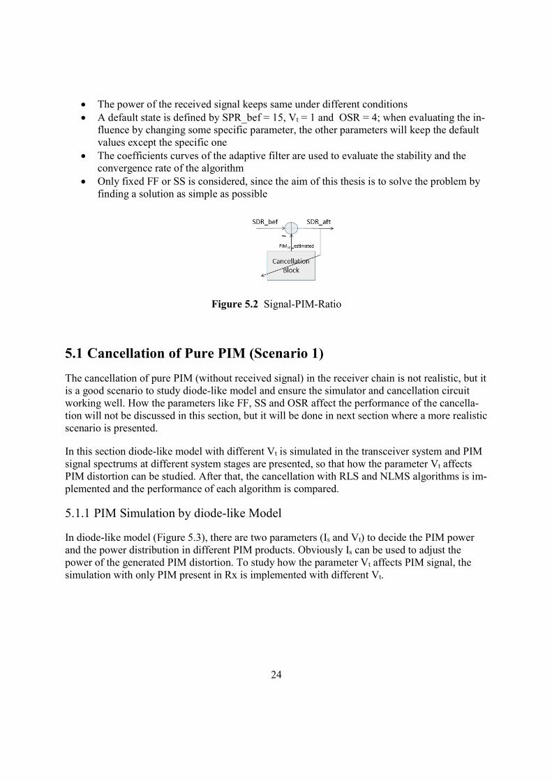
Figure 5.2 Signal-PIM-Ratio
5.1 Cancellation of Pure PIM (Scenario 1)
The cancellation of pure PIM (without received signal) in the receiver chain is not realistic, but it is a good scenario to study diode-like model and ensure the simulator and cancellation circuit working well. How the parameters like FF, SS and OSR affect the performance of the cancella-tion will not be discussed in this section, but it will be done in next section where a more realistic scenario is presented.
In this section diode-like model with different Vt is simulated in the transceiver system and PIM signal spectrums at different system stages are presented, so that how the parameter Vt affects PIM distortion can be studied. After that, the cancellation with RLS and NLMS algorithms is im-plemented and the performance of each algorithm is compared.
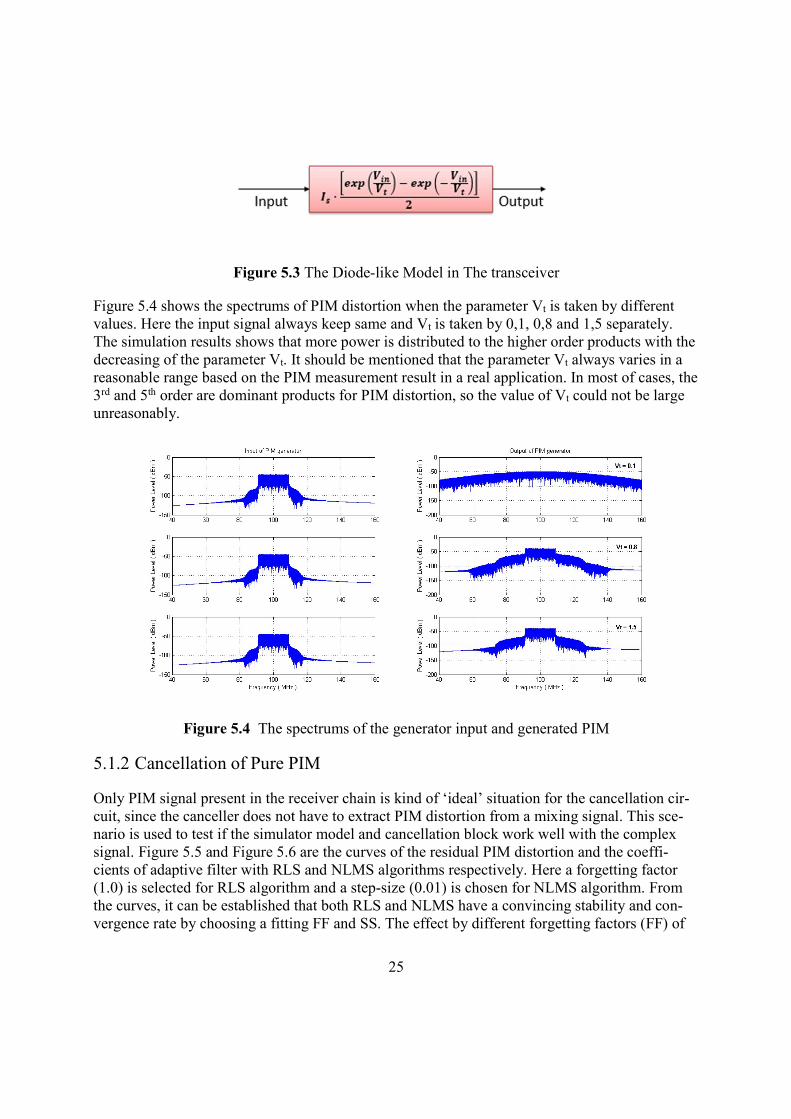
5.1.1 PIM Simulation by diode-like Model
In diode-like model (Figure 5.3), there are two parameters (Is and Vt) to decide the PIM power and the power distribution in different PIM products. Obviously Is can be used to adjust the power of the generated PIM distortion. To study how the parameter Vt affects PIM signal, the simulation with only PIM present in Rx is implemented with different Vt.
25
Figure 5.3 The Diode-like Model in The transceiver
Figure 5.4 shows the spectrums of PIM distortion when the parameter Vt is taken by different values. Here the input signal always keep same and Vt is taken by 0,1, 0,8 and 1,5 separately. The simulation results shows that more power is distributed to the higher order products with the decreasing of the parameter Vt. It should be mentioned that the parameter Vt always varies in a reasonable range based on the PIM measurement result in a real application. In most of cases, the 3rd and 5th order are dominant products for PIM distortion, so the value of Vt could not be large unreasonably.
Figure 5.4 The spectrums of the generator input and generated PIM
5.1.2 Cancellation of Pure PIM
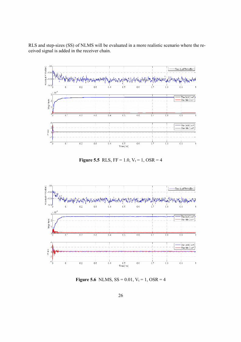
Only PIM signal present in the receiver chain is kind of ‘ideal’ situation for the cancellation cir-cuit, since the canceller does not have to extract PIM distortion from a mixing signal. This sce-nario is used to test if the simulator model and cancellation block work well with the complex signal. Figure 5.5 and Figure 5.6 are the curves of the residual PIM distortion and the coeffi-cients of adaptive filter with RLS and NLMS algorithms respectively. Here a forgetting factor (1.0) is selected for RLS algorithm and a step-size (0.01) is chosen for NLMS algorithm. From the curves, it can be established that both RLS and NLMS have a convincing stability and con-vergence rate by choosing a fitting FF and SS. The effect by different forgetting factors (FF) of
26
RLS and step-sizes (SS) of NLMS will be evaluated in a more realistic scenario where the re-ceived signal is added in the receiver chain.
Figure 5.5 RLS, FF = 1.0, Vt = 1, OSR = 4
Figure 5.6 NLMS, SS = 0.01, Vt = 1, OSR = 4
27
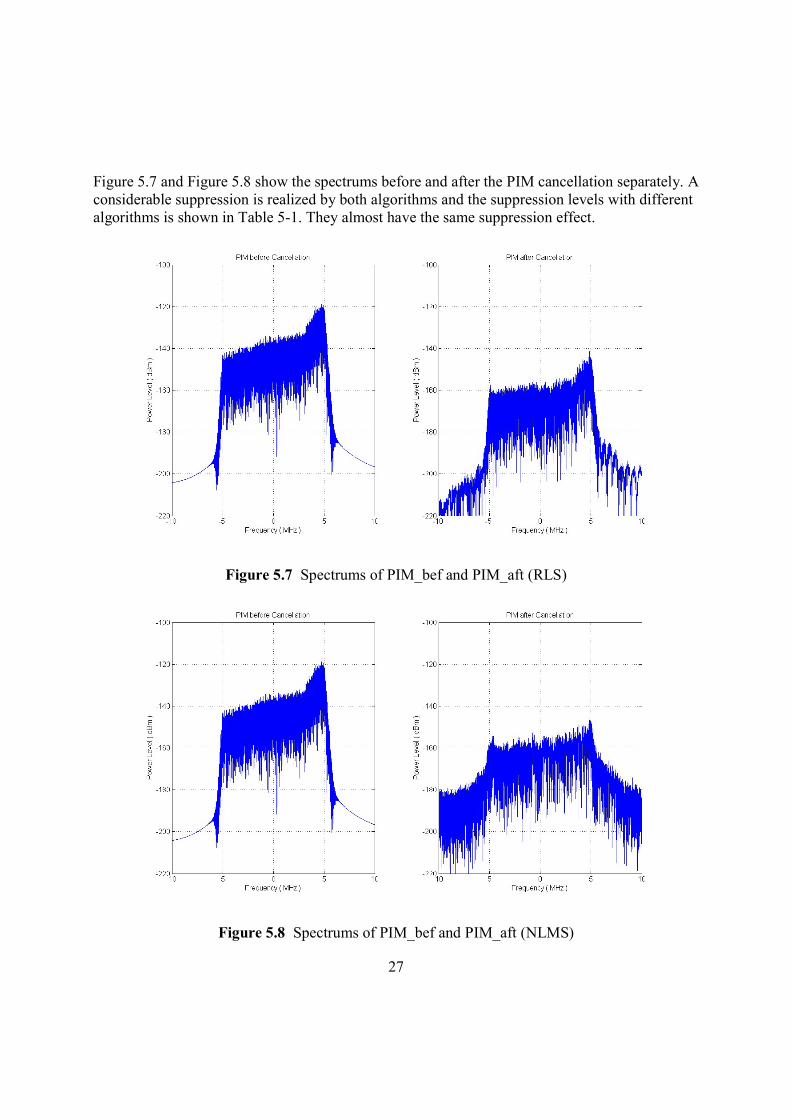
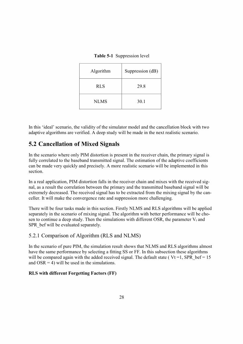
Figure 5.7 and Figure 5.8 show the spectrums before and after the PIM cancellation separately. A considerable suppression is realized by both algorithms and the suppression levels with different algorithms is shown in Table 5-1. They almost have the same suppression effect.
Figure 5.7 Spectrums of PIM_bef and PIM_aft (RLS)
Figure 5.8 Spectrums of PIM_bef and PIM_aft (NLMS)
28
Table 5-1 Suppression level
Algorithm Suppression (dB)
RLS 29.8
NLMS 30.1
In this ‘ideal’ scenario, the validity of the simulator model and the cancellation block with two adaptive algorithms are verified. A deep study will be made in the next realistic scenario.
5.2 Cancellation of Mixed Signals
In the scenario where only PIM distortion is present in the receiver chain, the primary signal is fully correlated to the baseband transmitted signal. The estimation of the adaptive coefficients can be made very quickly and precisely. A more realistic scenario will be implemented in this section.
In a real application, PIM distortion falls in the receiver chain and mixes with the received sig-nal, as a result the correlation between the primary and the transmitted baseband signal will be extremely decreased. The received signal has to be extracted from the mixing signal by the can-celler. It will make the convergence rate and suppression more challenging.
There will be four tasks made in this section. Firstly NLMS and RLS algorithms will be applied separately in the scenario of mixing signal. The algorithm with better performance will be cho-sen to continue a deep study. Then the simulations with different OSR, the parameter Vt and SPR_bef will be evaluated separately.
5.2.1 Comparison of Algorithm (RLS and NLMS)
In the scenario of pure PIM, the simulation result shows that NLMS and RLS algorithms almost have the same performance by selecting a fitting SS or FF. In this subsection these algorithms will be compared again with the added received signal. The default state ( Vt =1, SPR_bef = 15 and OSR = 4) will be used in the simulations.
RLS with different Forgetting Factors (FF)
29
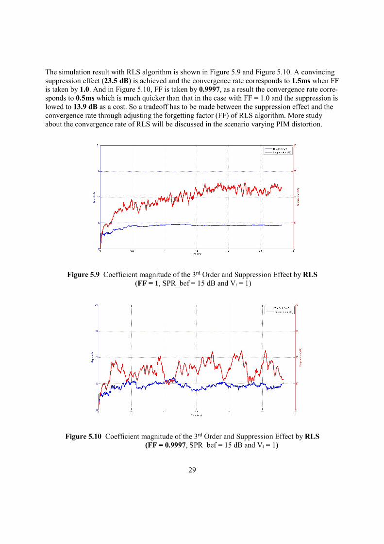
The simulation result with RLS algorithm is shown in Figure 5.9 and Figure 5.10. A convincing suppression effect (23.5 dB) is achieved and the convergence rate corresponds to 1.5ms when FF is taken by 1.0. And in Figure 5.10, FF is taken by 0.9997, as a result the convergence rate corre-sponds to 0.5ms which is much quicker than that in the case with FF = 1.0 and the suppression is lowed to 13.9 dB as a cost. So a tradeoff has to be made between the suppression effect and the convergence rate through adjusting the forgetting factor (FF) of RLS algorithm. More study about the convergence rate of RLS will be discussed in the scenario varying PIM distortion.
Figure 5.9 Coefficient magnitude of the 3rd Order and Suppression Effect by RLS (FF = 1, SPR_bef = 15 dB and Vt = 1)
Figure 5.10 Coefficient magnitude of the 3rd Order and Suppression Effect by RLS (FF = 0.9997, SPR_bef = 15 dB and Vt = 1)
30
NLMS with different Step-Size (SS)
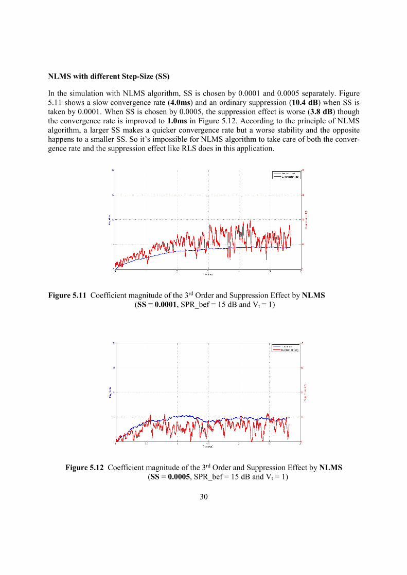
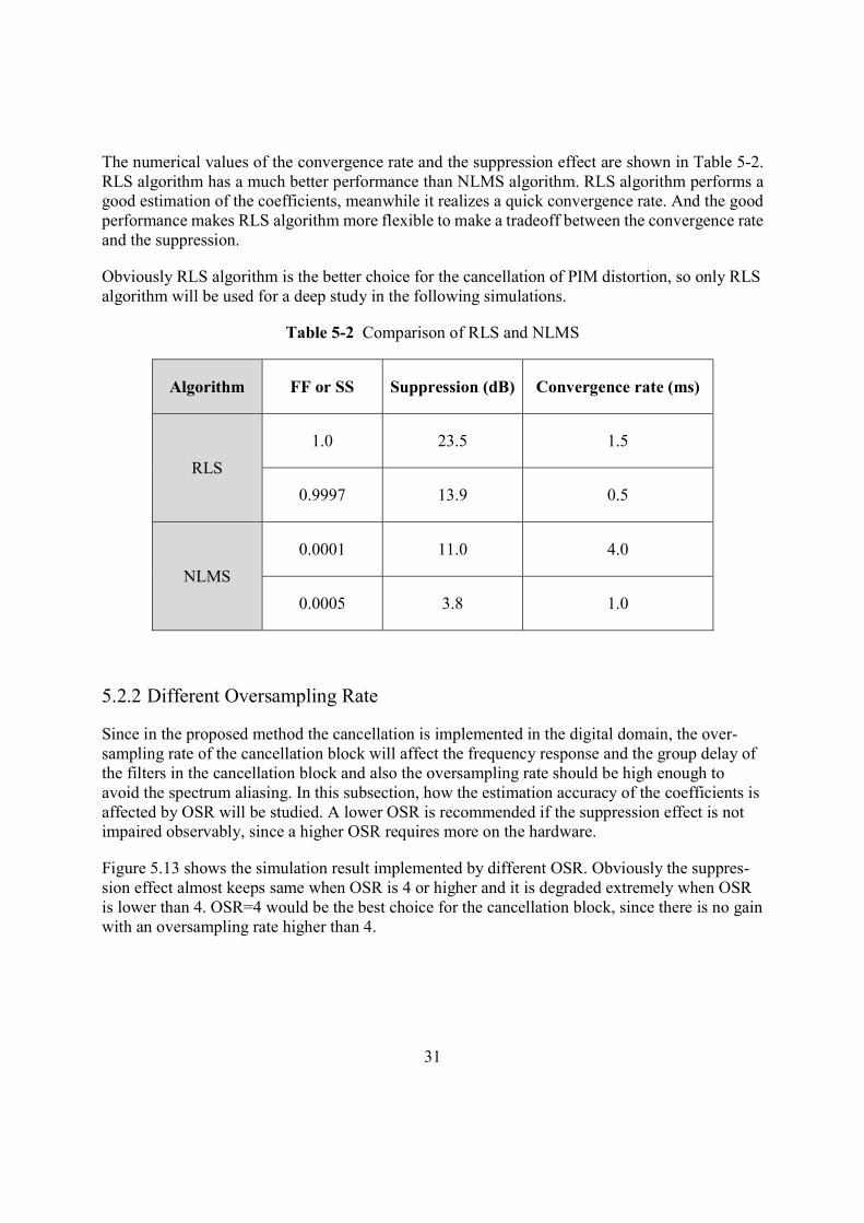
In the simulation with NLMS algorithm, SS is chosen by 0.0001 and 0.0005 separately. Figure 5.11 shows a slow convergence rate (4.0ms) and an ordinary suppression (10.4 dB) when SS is taken by 0.0001. When SS is chosen by 0.0005, the suppression effect is worse (3.8 dB) though the convergence rate is improved to 1.0ms in Figure 5.12. According to the principle of NLMS algorithm, a larger SS makes a quicker convergence rate but a worse stability and the opposite happens to a smaller SS. So it’s impossible for NLMS algorithm to take care of both the conver-gence rate and the suppression effect like RLS does in this application.
Figure 5.11 Coefficient magnitude of the 3rd Order and Suppression Effect by NLMS (SS = 0.0001, SPR_bef = 15 dB and Vt = 1)
Figure 5.12 Coefficient magnitude of the 3rd Order and Suppression Effect by NLMS (SS = 0.0005, SPR_bef = 15 dB and Vt = 1)
31
The numerical values of the convergence rate and the suppression effect are shown in Table 5-2. RLS algorithm has a much better performance than NLMS algorithm. RLS algorithm performs a good estimation of the coefficients, meanwhile it realizes a quick convergence rate. And the good performance makes RLS algorithm more flexible to make a tradeoff between the convergence rate and the suppression.
Obviously RLS algorithm is the better choice for the cancellation of PIM distortion, so only RLS algorithm will be used for a deep study in the following simulations.
Table 5-2 Comparison of RLS and NLMS
Algorithm FF or SS Suppression (dB) Convergence rate (ms)
RLS
1.0 23.5 1.5
0.9997 13.9 0.5
NLMS
0.0001 11.0 4.0
0.0005 3.8 1.0
5.2.2 Different Oversampling Rate
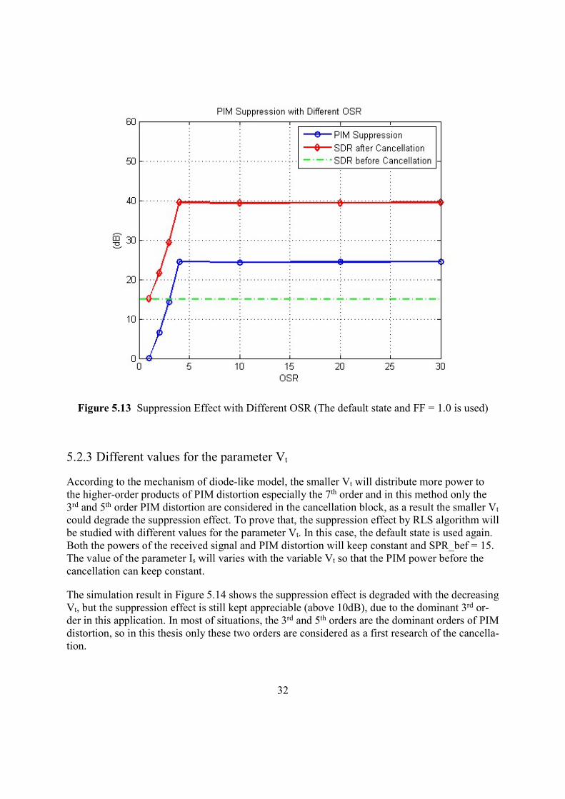
Since in the proposed method the cancellation is implemented in the digital domain, the over-sampling rate of the cancellation block will affect the frequency response and the group delay of the filters in the cancellation block and also the oversampling rate should be high enough to avoid the spectrum aliasing. In this subsection, how the estimation accuracy of the coefficients is affected by OSR will be studied. A lower OSR is recommended if the suppression effect is not impaired observably, since a higher OSR requires more on the hardware.
Figure 5.13 shows the simulation result implemented by different OSR. Obviously the suppres-sion effect almost keeps same when OSR is 4 or higher and it is degraded extremely when OSR is lower than 4. OSR=4 would be the best choice for the cancellation block, since there is no gain with an oversampling rate higher than 4.
32
Figure 5.13 Suppression Effect with Different OSR (The default state and FF = 1.0 is used)
5.2.3 Different values for the parameter Vt
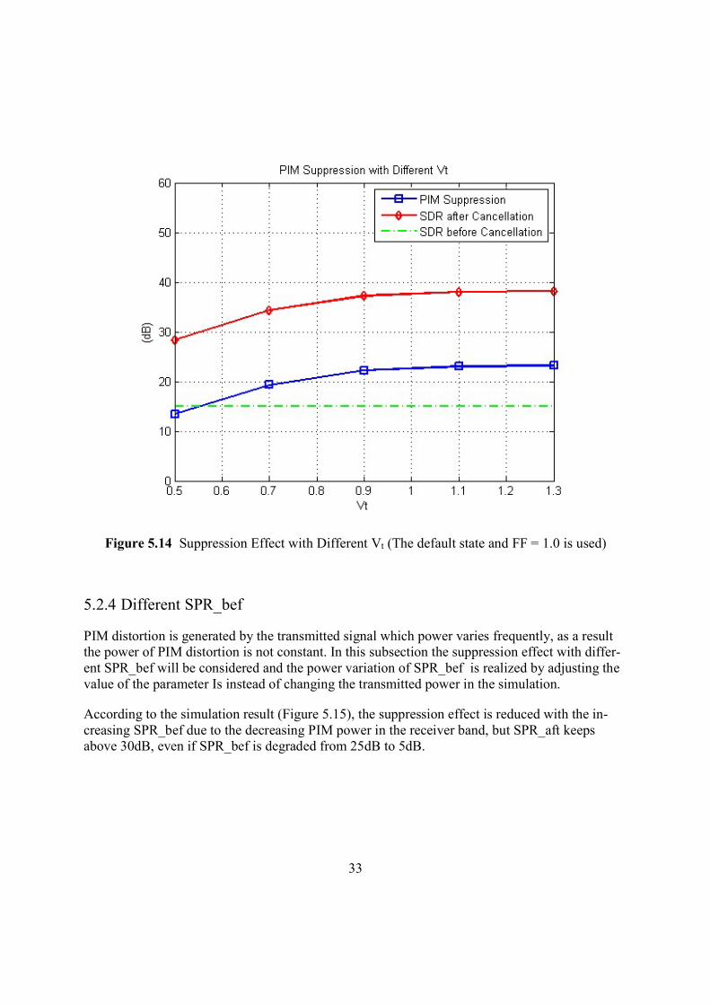
According to the mechanism of diode-like model, the smaller Vt will distribute more power to the higher-order products of PIM distortion especially the 7th order and in this method only the 3rd and 5th order PIM distortion are considered in the cancellation block, as a result the smaller Vt could degrade the suppression effect. To prove that, the suppression effect by RLS algorithm will be studied with different values for the parameter Vt. In this case, the default state is used again. Both the powers of the received signal and PIM distortion will keep constant and SPR_bef = 15. The value of the parameter Is will varies with the variable Vt so that the PIM power before the cancellation can keep constant.
The simulation result in Figure 5.14 shows the suppression effect is degraded with the decreasing Vt, but the suppression effect is still kept appreciable (above 10dB), due to the dominant 3rd or-der in this application. In most of situations, the 3rd and 5th orders are the dominant orders of PIM distortion, so in this thesis only these two orders are considered as a first research of the cancella-tion.
33
Figure 5.14 Suppression Effect with Different Vt (The default state and FF = 1.0 is used)
5.2.4 Different SPR_bef
PIM distortion is generated by the transmitted signal which power varies frequently, as a result the power of PIM distortion is not constant. In this subsection the suppression effect with differ-ent SPR_bef will be considered and the power variation of SPR_bef is realized by adjusting the value of the parameter Is instead of changing the transmitted power in the simulation.
According to the simulation result (Figure 5.15), the suppression effect is reduced with the in-creasing SPR_bef due to the decreasing PIM power in the receiver band, but SPR_aft keeps above 30dB, even if SPR_bef is degraded from 25dB to 5dB.
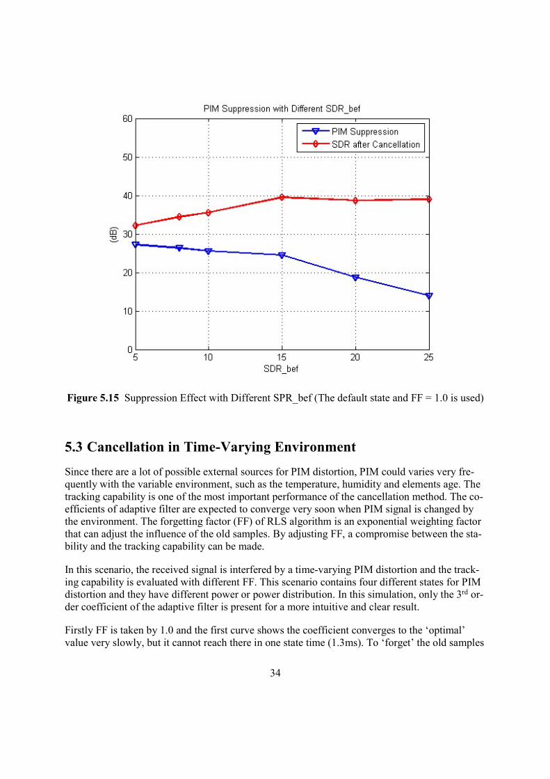
34
Figure 5.15 Suppression Effect with Different SPR_bef (The default state and FF = 1.0 is used)
5.3 Cancellation in Time-Varying Environment
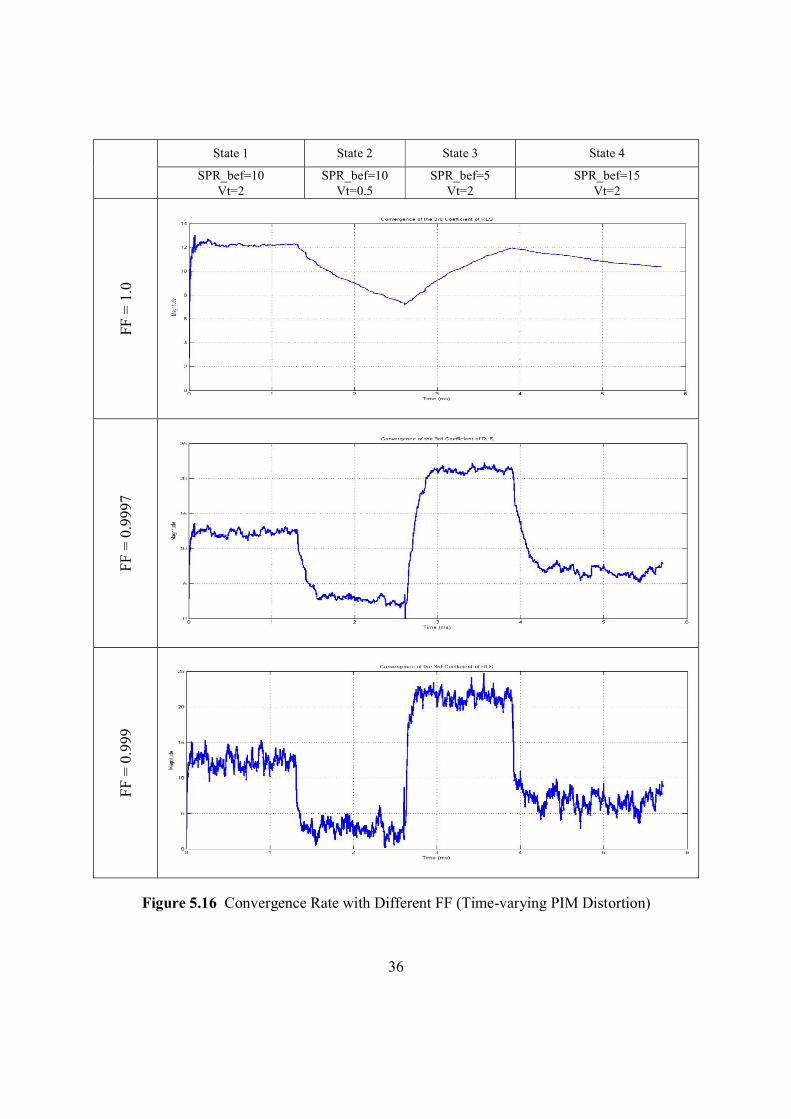
Since there are a lot of possible external sources for PIM distortion, PIM could varies very fre-quently with the variable environment, such as the temperature, humidity and elements age. The tracking capability is one of the most important performance of the cancellation method. The co-efficients of adaptive filter are expected to converge very soon when PIM signal is changed by the environment. The forgetting factor (FF) of RLS algorithm is an exponential weighting factor that can adjust the influence of the old samples. By adjusting FF, a compromise between the sta-bility and the tracking capability can be made.
In this scenario, the received signal is interfered by a time-varying PIM distortion and the track-ing capability is evaluated with different FF. This scenario contains four different states for PIM distortion and they have different power or power distribution. In this simulation, only the 3rd or-der coefficient of the adaptive filter is present for a more intuitive and clear result.
Firstly FF is taken by 1.0 and the first curve shows the coefficient converges to the ‘optimal’ value very slowly, but it cannot reach there in one state time (1.3ms). To ‘forget’ the old samples

35
effect gradually, the forgetting factor is taken by 0.9997 and 0.999 separately. The simulation re-sult shows the tracking capability is improved significantly. The convergence time corresponds to 0.3ms when FF is chosen by 0.9997 and it is lowered to 0.15ms when FF is chosen by 0.999. Both of them are shorter than one time slot if FDD LTE system is assumed and there is enough margin to make a tradeoff between the tracking capability and stead state.
36
State 1 State 2 State 3 State 4
SPR_bef=10 Vt=2
SPR_bef=10 Vt=0.5
SPR_bef=5 Vt=2
SPR_bef=15 Vt=2
FF =
1.0
FF =
0.9
997
FF
= 0
.999
Figure 5.16 Convergence Rate with Different FF (Time-varying PIM Distortion)
37
6 Conclusion
This thesis presented a cancellation technique to suppress PIM distortion in the digital domain. As the key part of the technique, adaptive filter was used to estimate the coefficients, compensate for the phase distortion and track the PIM variation in real time. The algorithms RLS and NLMS were explored and compared in this work to get an optimal solution. Also a lower oversampling rate realizations was required in the cancellation block.
RLS algorithm performs much better than NLMS when the received signal is interfered by PIM distortion, though both these two algorithms have a significant suppression when only PIM dis-tortion is present in the receiver chain. And forgetting factor make RLS algorithm very flexible to make a tradeoff between the convergence rate and the stead-state. After an overall comparison and analysis, RLS was chosen as the adaptive algorithm for this technique.
A lower sampling rate was realized for the cancellation circuit without any degradation on the performance. From the power dissipation point of view a low sampling rate benefits the hard-ware.
In this proposed technique, only the 3rd and 5th order of PIM distortion are considered for the suppression. The suppression effect was evaluated when the higher orders especially the 7th product of PIM distortion were distributed with more or less power portion. The simulation re-sult shows that the suppression always kept a convincing effect if a reasonable power distribution is applied, though the effect was impaired with the increasing power of the higher orders.
A good signal-PIM-ratio after the cancelation (SPR_aft) is expected, even though the original signal-PIM-ratio (SPR_bef) is poor. The simulation shows that SPR_aft was always improved to be over 30dB, even if the SPR_bef is down to 5dB.
Time-dependency of PIM distortion is always a big challenge for the suppression, but in this method the flexibility of forgetting factor of RLS algorithm offers a great solution on this prob-lem. A good tracking capability can be realized when the forgetting factor is lowed a little bit from 1.0 to 0.9997. Though the tracking capability is realized at the cost of the suppression ef-fect, it is tolerable.
To ensure the overall goal of the project has reached, many simulations have been made under different situations in this thesis. The method provides both a good convergence rate and sup-pression effect. Additionally a good tracking capability was also realized by a fitting forgetting factor. As a first research of this cancellation technique, the simulation results meet the expecta-tions.
As the future work, the cancellation of the 7th even higher orders of PIM distortion should be considered and some more imperfections from the transceiver system and the environment

38
should be involved in the simulation. Besides that, this technique should be implemented and verified in the hardware.

39
Appendix A
Taylor Series for exponential function
Taylor Series can be written as
f( ) +( )
1!( − ) +
( )
2!( − ) +
( )
3!( − ) + ⋯
or
( )( )
!( − )
where n! denotes the factorial of n and ( )( ) denotes the nth derivative of the f evaluated at the point a.
The Taylor series for the exponential function exp(x) at the point a=0 can be expressed as
0!+
1!+
2!+
3!… =
!= 1 + +
2+
6+
24+
120…
The Taylor series for the function exp(x)-exp(-x) at the point a=0 can be expressed as
+6
+120
…
Only the odd products are left.
40
Appendix B
The Structure of LTE FDD Frame
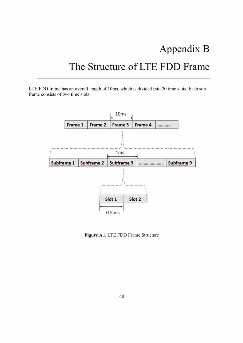
LTE FDD frame has an overall length of 10ms, which is divided into 20 time slots. Each sub frame consists of two time slots.
Figure A.1 LTE FDD Frame Structure
41
Appendix C
More Simulation Results
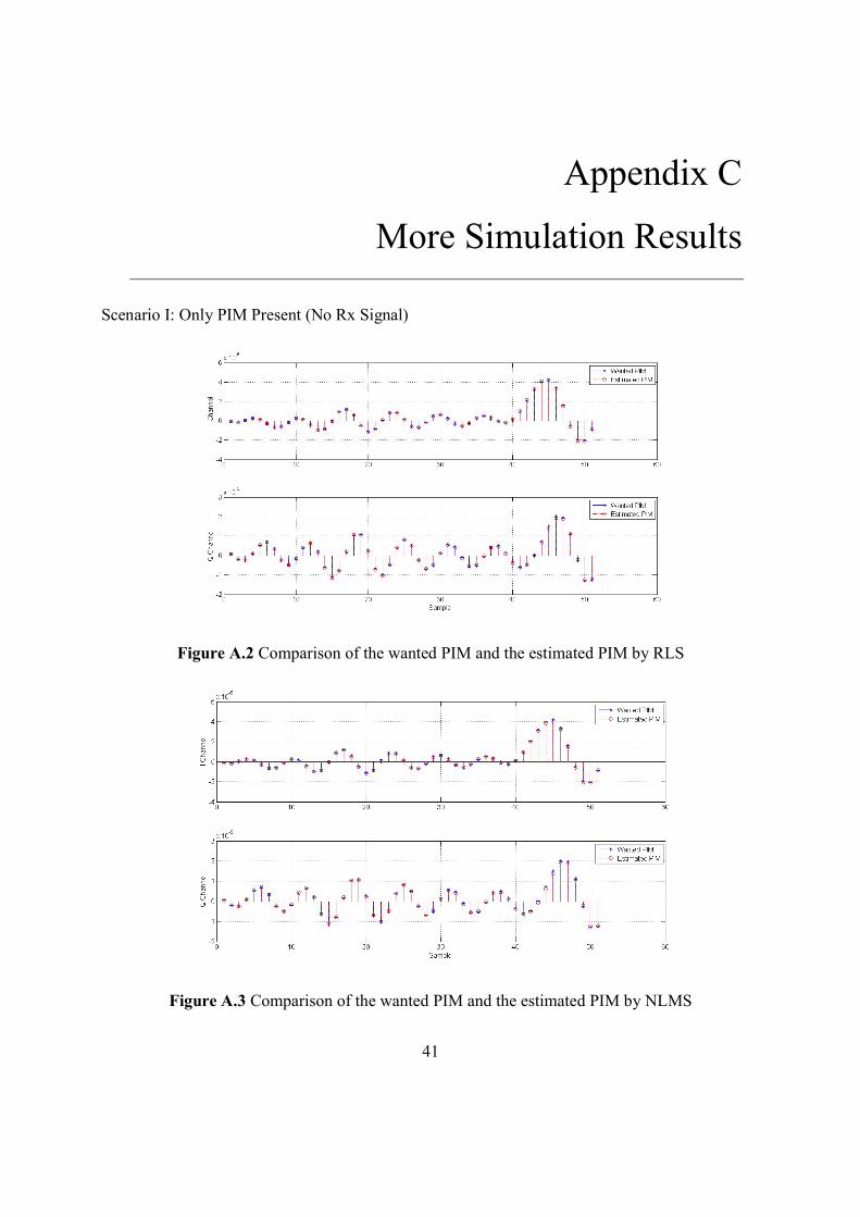
Scenario I: Only PIM Present (No Rx Signal)
Figure A.2 Comparison of the wanted PIM and the estimated PIM by RLS
Figure A.3 Comparison of the wanted PIM and the estimated PIM by NLMS
42
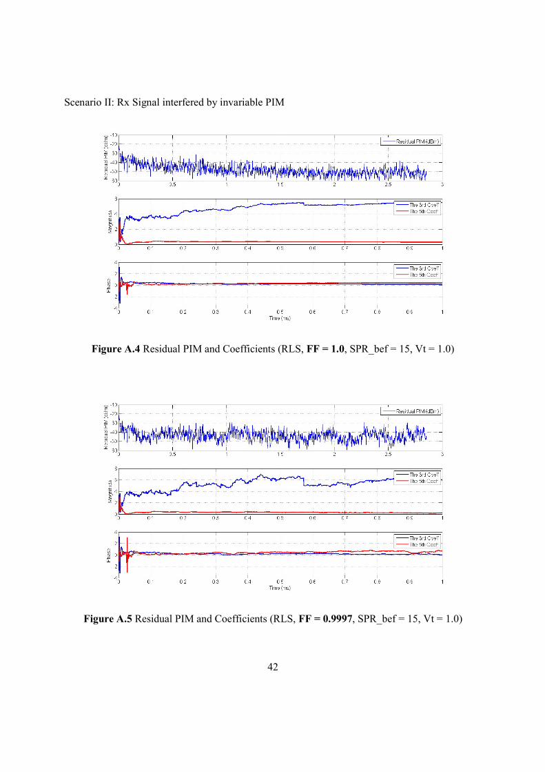
Scenario II: Rx Signal interfered by invariable PIM
Figure A.4 Residual PIM and Coefficients (RLS, FF = 1.0, SPR_bef = 15, Vt = 1.0)
Figure A.5 Residual PIM and Coefficients (RLS, FF = 0.9997, SPR_bef = 15, Vt = 1.0)
43
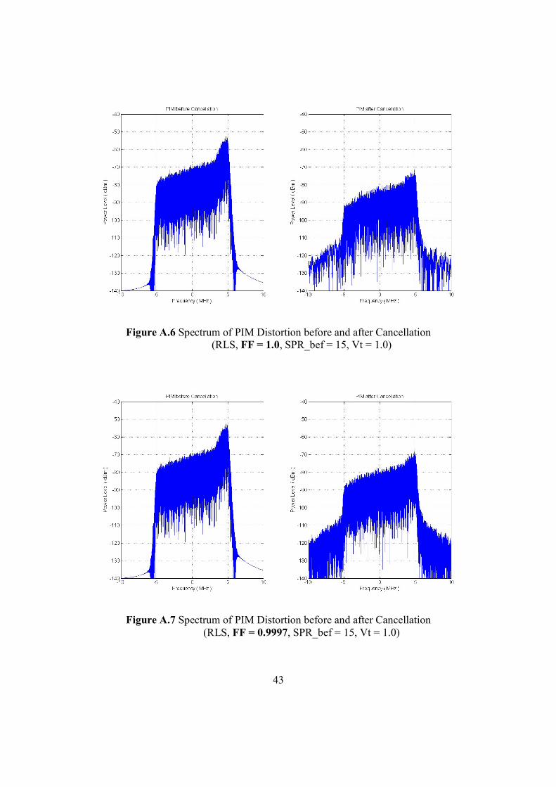
Figure A.6 Spectrum of PIM Distortion before and after Cancellation (RLS, FF = 1.0, SPR_bef = 15, Vt = 1.0)
Figure A.7 Spectrum of PIM Distortion before and after Cancellation (RLS, FF = 0.9997, SPR_bef = 15, Vt = 1.0)
44
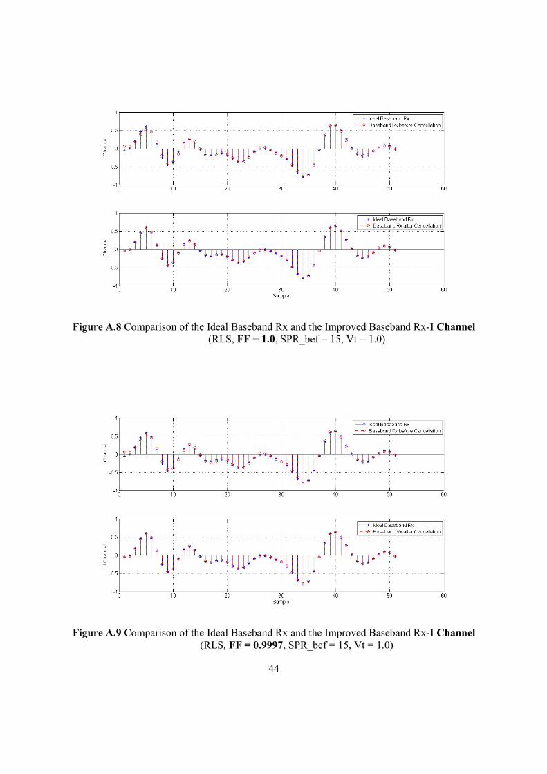
Figure A.8 Comparison of the Ideal Baseband Rx and the Improved Baseband Rx-I Channel (RLS, FF = 1.0, SPR_bef = 15, Vt = 1.0)
Figure A.9 Comparison of the Ideal Baseband Rx and the Improved Baseband Rx-I Channel (RLS, FF = 0.9997, SPR_bef = 15, Vt = 1.0)
45
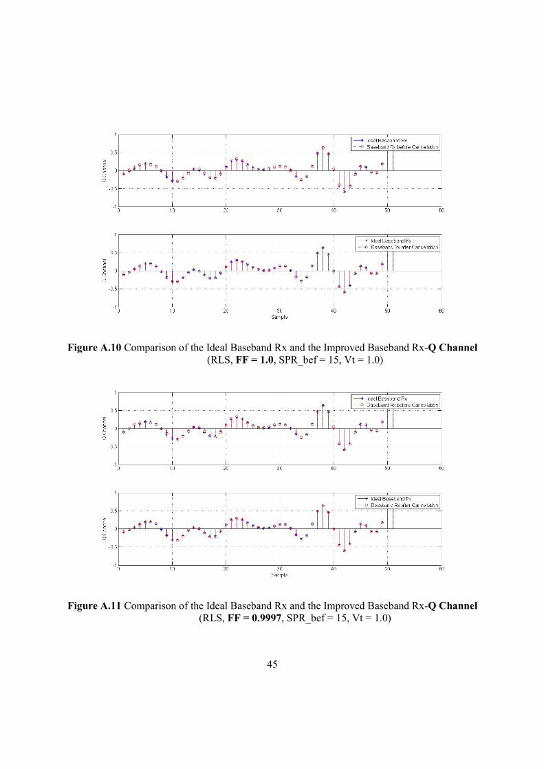
Figure A.10 Comparison of the Ideal Baseband Rx and the Improved Baseband Rx-Q Channel (RLS, FF = 1.0, SPR_bef = 15, Vt = 1.0)
Figure A.11 Comparison of the Ideal Baseband Rx and the Improved Baseband Rx-Q Channel (RLS, FF = 0.9997, SPR_bef = 15, Vt = 1.0)
46
References
[1] Paulo Sergio Ramirez Adaptive Filtering, Springer US, 2002
[2] G. C. Goodwin and R. L. Payne Dynamic System Identification: Experiment Design and Data Analysis, Academic Press, New York, NY, 1977.
[3] Adnan Kiayani, Student Member, IEEE, Lauri Anttila, Member, IEEE, and Mikko Valkama, Member; IEEE Digital Suppression of Power Amplifier Spurious Emissions at Receiver Band in FDD Transceivers, 2014
[4] Adnan Kiayani, Mahmoud Abdelaziz, Lauri Anttila and Mikko Valkama Digital Mitigation of Transmitter-Induced Receiver Desensitization in Carrier Aggrega-tion FDD Transceivers, 2015
[5] Thomas Ahlström, Claes Bengtsson Digital Interference Cancellation in a Full Duplex System, 2008
[6] Adaptive Filter, https://en.wikipedia.org/wiki/Adaptive_filter [7] Sami Heinonen
Students on Microwave Antennas: Passive Inter-modulation Distortion in Antenna Struc-tures and Design ofMicrostrip Antenna Elements, 2005
[8] Jiang Jie, Li Tuanjie, Ma Xiaofei and Wang Pel A Nonlinear Circuit Equivalent Circuit Method for Analysis of Passive Inter-modulation of Mesh Reflectors, 2014
[9] Jiang-hu Jiang, Shi-quan Zhang, Shao-zhou Wu, Gang Ba Prediction of Passive Inter-modulation Power Level Based on Double Exponential Func-tion Model and Genetic Algorithm, 2011
[10] Krzysztof Dufrene Analysis and Cancellation Method of Second Order Intermodulation Distortion in RFIC Downconversion Mixers, 2007
[11] Raja Abid Asghar, Abu Zar Matlab Simulator for Adaptive Filters
[12] Christian Lederer, Mario Huemer Simplified complex LMS algorithm for the cancellation of second-order TX intermodula-tion distortions in homodyne receivers,2011
[13] Hayg-Taniel Dabag, Hamed Gheidi, Prasad Gudem, Peter M, Asbeck All-Digital Cancellatoin Technique To Mitigate Self-Jamming In Uplink Carrier Aggre-gation In Cellular Handset, 2013
[14] Dani Korpi, Yang-Seok Choi, Timo Huusari, Larti Anttila,Shilpa Talwar, and Mikko Valkama Adaptive Nonlinear Digital Self-interference Cancellation for Mobile Inband Full-Duplex Radio: Algorithms and RF Measurements, 2016
[15] M.Omer, R.Rimini, P.Heidmann, and J.S. Kenney

47
A Compensation Scheme to Allow Full Duplex Operation in the Presence of Highly Non-linear Microwave Components for 4G systems, 2011
[16] Dani Korpi, Lauri Anttila, and Mikko Valkama Reference Receiver Based Digital Self-Interference Cancellation in MIMO Full-Duplex Transceivers, 2014
[17] Shruti R Patel,Sandip R Panchal, Hiren Mewada Comparative Study of LMS & RLS Algorithms for Adaptive Filter Design with FPGA, 2014

Passive Inter-modulation Cancellationin FDD System
FAN CHENMASTER´S THESISDEPARTMENT OF ELECTRICAL AND INFORMATION TECHNOLOGY |FACULTY OF ENGINEERING | LTH | LUND UNIVERSITY
Printed by Tryckeriet i E-huset, Lund 2017
FAN
CH
ENPassive Inter-m
odulation Cancellation in FD
D System
LUN
D 2017
Series of Master’s thesesDepartment of Electrical and Information Technology
LU/LTH-EIT 2017-563
http://www.eit.lth.se