SIAM J. MATRIX ANAL. APPL. c\bigcirc 2018 Society for Industrial and Applied MathematicsVol. 39, No. 4, pp. 1726--1749

PATH-FOLLOWING METHOD TO DETERMINE THE FIELD OFVALUES OF A MATRIX WITH HIGH ACCURACY\ast

S\'EBASTIEN LOISEL\dagger AND PETER MAXWELL\ddagger

\bfA \bfb \bfs \bft \bfr \bfa \bfc \bft . We describe a novel and efficient algorithm for calculating the field of values bound-ary, \partial W(\cdot ), of an arbitrary complex square matrix: the boundary is described by a system of ordinarydifferential equations which are solved using Runge--Kutta (Dormand--Prince) numerical integrationto obtain control points with derivatives, then finally Hermite interpolation is applied to producea dense output. The algorithm computes \partial W(\cdot ) both efficiently and with low error. Formal errorbounds are proven for specific classes of matrix. Furthermore, we summarize the existing state of theart and make comparisons with the new algorithm. Finally, numerical experiments are performed toquantify the cost-error trade-off between the new algorithm and existing algorithms.

\bfK \bfe \bfy \bfw \bfo \bfr \bfd \bfs . field of values, numerical range, Johnson's algorithm, Runge--Kutta, Dormand--Prince, parametrized eigenvalue problem, eigenvalue perturbation, eigenvalue crossing

\bfA \bfM \bfS \bfs \bfu \bfb \bfj \bfe \bfc \bft \bfc \bfl \bfa \bfs \bfs \bfi fi\bfc \bfa \bft \bfi \bfo \bfn \bfs . 15A18, 15A60, 15B57, 65F15, 65F30

\bfD \bfO \bfI . 10.1137/17M1148608

1. Introduction. For a complex matrix A \in \BbbC n\times n, the field of values or nu-merical range W(A) is the image of the unit sphere under the Rayleigh quotient ofthe matrix:

W(A) := \{ \bfitx \ast A\bfitx : \bfitx \in \BbbC n, \bfitx \ast \bfitx = 1 \} .

The field of values encloses the set of eigenvalues and can be used in a similarmanner as the set of eigenvalues, e.g., to estimate the magnitude of matrix functions[10]; see also [44, p. 167]. Our interest is in finite-dimensional complex matrices.However, W(A) can also be defined in a similar manner when A is an operator actingon a general Hilbert space [21, p. 1].

The problem of calculating the field of values boundary, \partial W(A), has a long history,with the canonical algorithm surely being that of Johnson [26], but see also [36] and[28], [14]. We now briefly outline Johnson's algorithm. For a given matrix A \in \BbbC n\times n,define H(eitA) := 1

2 (eitA+ e - itA\ast ). H(eitA), being Hermitian, has real eigenvalues.

Let \lambda max(t) denote the largest eigenvalue of H(eitA), and let \bfitu max(t) denote a cor-responding unit eigenvector. Then, Johnson's function \zeta (t) = \bfitu max(t)

\ast A\bfitu max(t) isa parametrization of \partial W(A) for t \in [0, 2\pi ). Although \partial W(A) is continuous with atmost n points of discontinuous first derivative (see subsection 2.2), continuity does notnecessarily hold for the parametrization \zeta (t); indeed, this was alluded to in Johnson'spaper [26], e.g., Theorem 3. If, for a given value of t = tk, the eigenvalue \lambda max(tk)is nonsimple, then there are multiple linearly independent choices of \bfitu max(tk), each,possibly, producing a different value of \zeta (tk). Therefore, there can be a jump discon-tinuity at tk where \zeta (tk) is not well-defined but each of the one-sided limits \zeta (t+k ) and

\ast Received by the editors September 21, 2017; accepted for publication (in revised form) by M. A.Freitag September 13, 2018; published electronically November 27, 2018.

http://www.siam.org/journals/simax/39-4/M114860.html\bfF \bfu \bfn \bfd \bfi \bfn \bfg : The second author was funded by the Norwegian Research Council (FRINATEK),

project 249740.\dagger Department of Mathematics, Heriot-Watt University, Edinburgh, Scotland EH14 4AS, UK

(S.Loisel@hw.ac.uk).\ddagger Department of Energy and Process Engineering, Faculty of Engineering, NTNU--Norwegian

University of Science and Technology, Trondheim NO-7491, Norway (peter.maxwell@ntnu.no).

1726

PATH-FOLLOWING METHOD TO DETERMINE FIELD OF VALUES 1727

Fig. 1.1. A plot of the field of values of the matrix A = delsq(numgrid('S',20))+

0.1*randn(324) generated by the path-following algorithm. The red asterisks are the eigenvaluesof A, and the solid black line is the boundary of W(A). (Figure in color online.)

\zeta (t - k ) are well-defined; these tk correspond to, possibly degenerate, flat segments on\partial W(A). We show in Theorem 7.2 that there can be only finitely many such tk.

Johnson's algorithm is to sample \zeta (t) at discrete values tk = (k - 1)(2\pi /m), k =1, 2, . . . ,m, and approximate \partial W(A) by the polygon whose vertices are \{ \zeta (tk)\} mk=1,

where m \geq 3 is the number of vertices; we denote by \^\zeta (t) the piecewise linear approx-imation of \zeta (t) produced by Johnson's algorithm. Provided that one has an accurateand robust eigenvalue solver, Johnson's algorithm is able to approximate \partial W(A) for

sufficiently largem. The piecewise linear approximation \^\zeta (t) of \zeta (t) is exact at the ver-tices, with \scrO (m - 2) error between the vertices. Therefore, achieving approximationsof higher accuracy rapidly becomes prohibitively expensive. Several other algorithmsand strategies have been proposed to calculate the field of values boundary \partial W(A),e.g., Marcus and Pesce [34], Braconnier and Higham [4], and Uhlig [46].

Our main new idea is to use a ``path-following"" algorithm to efficiently computea high order near-interpolant \^\xi (t) of \zeta (t). This is possible because, from eigenvalueperturbation analysis, one can show that \zeta (t) is piecewise analytic. We derive a systemof differential equations for the parametrized eigenvalue problem H(eitA)\bfitu max(t) =\lambda max(t)\bfitu max(t) and, using a suitable ODE solver with dense output, obtain a high

order interpolant \^\xi (t) which approximates \zeta (t). Care must be taken to stop andrestart the ODE solver at points where \zeta (t) is less smooth, which we do in an efficientmanner. This feature makes our algorithm attractive compared to applying a highorder interpolant directly to Johnson's algorithm: without knowledge of where \zeta (t)is not smooth, the interpolant cannot achieve the anticipated accuracy. Johnsonobserves a similar result in his analysis at [26, p. 600]: he notes that ``flat"" portionsof \partial W(A) were not considered and may lead to slow convergence. An example ofthe piecewise polynomial approximation of \partial W(A) produced by the path-followingalgorithm can be seen in Figure 1.1; this is a 324 \times 324 matrix and the tolerance of

1728 S\'EBASTIEN LOISEL AND PETER MAXWELL

the ODE integrator was set to 10 - 10.The principal feature of our algorithm is that it computes W(A) more efficiently

than previous algorithms when the sought tolerance is small. Our analysis and nu-merical experiments reveal that the path-following algorithm is more efficient thanexisting algorithms in practical settings at moderate accuracy and is also asymptot-ically faster. Indeed, at high accuracy, our algorithm is at least an order of magni-tude faster. We also posit that our algorithm may have more generic applicabilityparticularly in relation to Sturm--Liouville problems; this is discussed further in theconclusions.

1.1. Related results using computational perturbation methods. Ourpath-following algorithm inherently adopts a perturbative or continuation approach.For context and without any aim of completeness, we make a very terse summary ofrelated results that the reader may find useful.

Lui [32] derives continuation methods based on inverse iteration and Lanczos forcalculation of pseudospectra. A homotopy method for solving the eigenproblem oflarge sparse real nonsymmetric matrices is given by Lui, Keller, and Kwok in [33].

In [19], Guglielmi and Overton describe an algorithm to calculate the pseudospec-tral abscissa and pseudospectral radius by using the rightmost eigenvalue of a sequenceof rank-1 updates Bk+1 = A+\varepsilon \bfity k\bfitx

\ast k, where \bfitx and \bfity are the leading ``RP-compatible""

left and right eigenvectors of Bk. In [17], [18], Guglielmi and Lubich observe thatGuglielmi and Overton's algorithm is an iterative algorithm on the manifold of nor-malized rank-1 matrices, \scrM = \{ \bfitu \bfitv \ast : \bfitu ,\bfitv \in \BbbC , \| \bfitu \| = \| \bfitv \| = 1 \} . By reframing theproblem as a continuous dynamical system on \scrM , a differential equation can be usedto solve for E(t) on \scrM such that the real part of the leading eigenvalue of A+ \varepsilon E(t)tends to the pseudospectral abscissa. In [29], Kressner and Vandereycken extend theresults of Guglielmi and Overton by using a subspace acceleration method.

In [3], Beyn and Th\"ummler create a predictor-corrector continuation method forinvariant subspaces (invariant pairs) of the quadratic eigenvalue problem with largesparse matrices depending on a single real parameter; they include several relevantand instructive practical applications. In [2], Beyn, Effenberger, and Kressner analyzeinvariant pairs for nonlinear eigenproblems which are entrywise holomorphic functionsin the eigenvalue parameter and describe a pseudoarclength predictor-corrector tech-nique for continuation of the invariant pairs.

Due to the philosophical relevance to the work herein, we also mention Sirkovi\'cand Kressner's result in [42] for approximating the smallest eigenvalue of a parameter-dependent Hermitian matrix.

1.2. Organization of the paper. Our paper is organized as follows. In sec-tion 2, we briefly recall the basic properties of the field of values and then reviewexisting algorithms in section 3. In section 4, we give a brief overview of our newalgorithm and clarify some properties of the Johnson parametrization in section 5.We fully specify the path-following algorithm in section 6. We provide analyses ofexpected eigenvalue crossings and error estimates in section 7. In section 8, we numer-ically compare the running time and accuracy of our new algorithm against severalexisting algorithms, including Johnson's algorithm. We end with some conclusions.

2. Basic properties of the field of values. The fundamental properties andresults concerning the field of values are more than adequately described in othersources [21], [24], [28], [14]. Nevertheless, we make use of some of these results herein,which shall be restated briefly without proof. The properties and results summarized

PATH-FOLLOWING METHOD TO DETERMINE FIELD OF VALUES 1729

in this section are in the context of our restricted finite-dimensional case only andmay not hold in a more general setting.

Definition 2.1 (Hermitian and skew-Hermitian parts of a matrix). For nota-tional convenience, we define

H(A) :=1

2(A+A\ast ) and S(A) :=

1

2(A - A\ast )

as the Hermitian and skew-Hermitian parts of the matrix, A. A matrix A can bewritten as A = H(A) + S(A).

Definition 2.2 (extremal eigenvalues). For Hermitian K \in \BbbC n\times n, we denotethe least and greatest eigenvalues by \lambda min(K) and \lambda max(K). For scalar t and squarematrix A, we define \lambda max(t) as the greatest eigenvalue of H(eitA).

2.1. Fundamental properties. Let A,B \in \BbbC n\times n.

Property 2.3.(a) The eigenvalues of A are contained within W(A), \sigma (A) \subseteq W(A);(b) the field of values is linear with respect to scaling and translation, W(\alpha A +

\beta I) = \alpha W(A) + \beta for all \alpha , \beta \in \BbbC , \alpha \not = 0;(c) unitary similarity invariance, W(U\ast AU) = W(A) for all unitary U \in \BbbC n\times n;(d) W(A) is compact (image of a compact set under a continuous function) [21,

p. 4], [24, p. 1];(e) W(A) is a convex set, cf. the Toeplitz--Hausdorff theorem [23], [43], and also

[11], [12], [20], [24], [37], [39];(f) \partial W(A), where n = 2 is a, possibly degenerate, ellipse, cf. elliptical range

theorem as described in [21, p. 3], Theorem 1.3.6a of [24, p. 23], and [31];(g) W(A) \subset \BbbR if and only if A is Hermitian, in other words W(A) is an inter-

val on the real line whenever A is Hermitian and, furthermore, \Re [W(A)] =W(H(A)) = [\lambda min(H(A)), \lambda max(H(A))];

(h) if A is normal, then W(A) = Co(\sigma (A)), in other words if A is normal, thenthe field of values is the convex hull of the eigenvalues (the converse is, ingeneral, not true for n > 4, cf. [25], [35]);

(i) for A1 \oplus A2 =\bigl[ A1 00 A2

\bigr] , A1 \in \BbbC n1\times n1 , A2 \in \BbbC n2\times n2 , then W(A1 \oplus A2) =

Co(W(A1)\bigcup

W(A2) ), the field of values of a direct sum of matrices is theconvex hull of the union of the field of values of those matrices; and

(j) for a multi-index, \bfitalpha = \{ \alpha 1, \alpha 2, . . . , \alpha k\} , define the principal submatrix of A asA(\bfitalpha ) being the rows and columns of A indexed by \bfitalpha then W(A(\bfitalpha )) \subseteq W(A).

2.2. ``Corners"" or ``sharp points"" of \bfpartial W(\bfitA ). Consider A \in \BbbC n\times n. \partial W(A)is smooth except possibly at a finite number of so-called ``sharp points"" or ``corners""which have nonunique tangents [24, p. 50], [21, p. 19] or, equivalently, where \partial W(A)is not a differentiable arc [12]. A sharp point of \partial W(A) must be an eigenvalue of Aalthough the converse does not necessarily hold; cf. Theorem 1 of [12] and Theorem1.5-5 of [21, p. 20]. Therefore, there are at most n sharp points on \partial W(A). Herein,we adopt the formal definition of a sharp point used in [24, p. 50].

Definition 2.4 (sharp point). A point \alpha \in \partial W(A) is a sharp point if there aret1 and t2 with 0 \leq t1 < t2 < 2\pi for which

\Re (eit\alpha ) = max\{ \Re (\beta ) : \beta \in W(eitA)\} for all t \in (t1, t2).

Sharp points can be characterized by Theorem 1.6.6 in [24] or Theorem 5 in [8].

1730 S\'EBASTIEN LOISEL AND PETER MAXWELL

Theorem 2.5. Let A \in \BbbC n\times n and \alpha \in \partial W(A). Then \alpha is a sharp point if andonly if A is unitarily similar to \alpha Im \oplus A1 with A1 \in \BbbC (n - m)\times (n - m) and \alpha /\in W(A1).In this case \alpha is the intersection of two flat line portions on \partial W(A).

3. Existing algorithms. There are only a handful of existing algorithms forcomputing the field of values boundary of a general complex matrix. The n = 2 casecan be trivially handled using the elliptical range theorem, Property 2.3 (f).

3.1. Johnson's algorithm. There is almost a de facto standard, published byJohnson in 1978 [26], for computing the field of values of a general complex squarematrix. The concept behind this method---taking advantage of the convexity propertyProperty 2.3 (e) of W(A) by successively applying a scalar rotation Property 2.3 (b) tothe matrix A then using the Hermitian projection property Property 2.3 (g) to boundthe field of values set between the least and greatest eigenvalues---has been expressedat least as far back as Murnaghan's terse result in 1932 [36] and Kippenhahn's morecomprehensive results in 1951 [28], [14]. However, Johnson's result is the first instanceof the method being used to create a convergent computational algorithm.

We will make use of this methodology, so we shall briefly recap the result from [26].Note that the Hermitian projection property Property 2.3 (g) states that \Re [W(A)] =[\lambda min(H(A)), \lambda max(H(A))]. Denote by \bfitu max an associated unit eigenvector for \lambda max.The line L = \{ \lambda max(H(A)) + is : s \in \BbbR \} defines a vertical support line tangent to\partial W(A). The intersection L \cap \partial W(A) may not be a single point as W(A) can have astraight line or ``flat"" segment along its boundary. Furthermore, where L and \partial W(A)intersect is also not necessarily on the real axis. The point

(3.1) p := \bfitu \ast maxA\bfitu max \in L \cap \partial W(A)

is on \partial W(A) with Figure 3.1a depicting this arrangement. Note, furthermore, thate - itW(eitA) = W(A). By successively applying a rotation by angle tk to A as eitkAfor k = \{ 1, . . . ,K\} , collecting the pk points for corresponding tk, and calculating theconvex hull will produce a piecewise linear inner boundary approximation for \partial W(A).Johnson takes this further by calculating an outer boundary using the supportinghyperplanes. This constrains \partial W(A) between an inner and outer boundary so thatan error bound can be calculated. This arrangement is depicted in Figure 3.1b.

3.2. Marcus--Pesce algorithm. An alternative method was described by Mar-cus and Pesce in 1987 [34] which involves using multiple random orthonormal ma-trix compressions of the form V \ast AV \in \BbbC 2\times 2 for V \in \BbbC n\times 2. For a matrix V =\bigl[ \bfitv 1 \bfitv 2 . . . \bfitv k] \in \BbbC n\times k, where the \bfitv i \in \BbbC n vectors form an orthonormal basis for Vand A \in \BbbC n\times n, the (matrix) compression of A is defined as

AV := V \ast AV,

where AV \in \BbbC k\times k. By using Property 2.3 (c) and Property 2.3 (j), it can be seenthat W(V \ast AV ) \subseteq W(A). Using the elliptical range theorem, Property 2.3 (f), whenk = 2, then W(V \ast AV ) is a, possibly degenerate, ellipse. In Theorem 1 of [34], it isproven that the field of values is equal to the union over all 2\times 2 matrix compressionsusing V = [\bfitv \bfone \bfitv \bftwo ], where \bfitv \bfone ,\bfitv \bftwo are real and orthonormal,

W(A) =\bigcup V

W(V \ast AV ).

Marcus and Pesce's computation strategy is essentially to pick a reasonable num-ber of random real orthonormal vector pairs, compute the resulting set of elliptical

PATH-FOLLOWING METHOD TO DETERMINE FIELD OF VALUES 1731

(a) Bounding of \partial W(A) using Hermitian partof matrix. Shown without rotation (t =0). The vertical bounding support line is indashed blue; the p point is marked with a redasterisk; and \partial W(A) in solid black.

(b) Illustration of an inner and outer Johnsonboundary for six rotation increments. Innerboundary is in dashed blue; outer boundaryis in dash-dotted magenta; outer supportinghyperplanes in dotted faint grey; eigenvaluesof A are shown with red asterisks; and exact\partial W(A) is in solid black.

Fig. 3.1. Plots showing how the Johnson algorithm bounds \partial W(A). (Figure in color online.)

(a) 12 ellipses: the Marcus--Pesce boundaryis a poor approximation of \partial W(A).

(b) 1000 ellipses: the Marcus--Pesce bound-ary is still showing high error.

Fig. 3.2. Figures akin to Uhlig's figure [46, Fig. 5] showing Marcus and Pesce's randomlygenerated eigenvectors for matrix compressions. The matrix compression ellipses are shown withthin black lines; the generated boundary in dashed blue; and exact \partial W(A) in solid black. (Figure incolor online.)

field of values sets, and then plot (or compute the convex hull and plot). This worksreasonably well for very small matrices but selecting vectors at random fails to ap-proximate the boundary accurately for matrices with n > 4; see Figure 3.2.

3.3. Uhlig's optimization of Marcus--Pesce. The strategy adopted by Uhlig[46] is faster and more accurate compared to the Marcus--Pesce method. Instead ofpicking random pairs of real orthonormal vectors, Uhlig proposes first calculating asmall number of ordered boundary points pk = \bfitu \ast

kA\bfitu k using Johnson's method andthen using successive eigenvector pairs from this list for the matrix compressions sothat each ellipse is more likely to constrain the boundary. In particular, Uhlig startsby constructing a so-called Bendixson box : for a particular tk, the greatest and leasteigenvalues from both the Hermitian and skew-Hermitian parts are used, which creates

1732 S\'EBASTIEN LOISEL AND PETER MAXWELL

(a) Uhlig's method quickly constrains theboundary: the generated boundary indashed blue is close to \partial W(A).

(b) A zoomed-in plot so that the generatedand true boundaries can be distinguished.

Fig. 3.3. Calculation of \partial W(A) using Uhlig's method for a random matrix A of size n = 5.Matrix compression ellipses can be seen internal to W(A). \partial W(A) is shown in solid black whereasthe boundary generated from the matrix compressions is in dashed blue. Eigenvalues are denotedwith red asterisks. (Figure in color online.)

a rectangular bounding box from the four initial eigenpairs. This initial list of fourvectors is then expanded by the judicious choice of further Johnson calculations, eachreturning two additional vectors---corresponding to the desired \lambda min and \lambda max---tomerge into the list. Uhlig proposed four rationales to choose these additional points[46, sect. 2.1]. Assuming the order of the vectors is maintained properly to representeither a clockwise or anticlockwise ordering, then once a suitable number of vectors arecollated, matrix compressions can be performed along the boundary. The algorithmsuccessively creates matrices Vk by picking the kth and (k + 1)th vector pair, with krunning over the full list, orthonormalizes the pair, calculates the matrix compressionAVk

, and then calculates a suitable number of points on the resulting field of valuesellipse. Finally, a convex hull is calculated on all the collected ellipse points to achievea boundary approximation as shown in Figure 3.3.

3.4. Braconnier--Higham approach. Braconnier and Higham applied a spe-cific implementation of the Lanczos algorithm for computing the field of values usingJohnson's method [4]. Their work focuses on optimizing the eigenproblem solves andapplying a continuation method. In this context, continuation means that when per-forming an eigenproblem solve using a Krylov subspace method one can often use theeigenvector from the previous result as the starting vector for the next computationin order to reduce the number of iterations required.

4. Algorithm overview. The strategy behind the new algorithm is to deter-mine \partial W(A) by ``tracking"" the dominant eigenpair of the Hermitian part of eitA asa function of t in an analogous manner to Johnson's method as described in subsec-tion 3.1. This can be expressed as

(4.1) H(eitA)\bfitu (t) = \lambda (t)\bfitu (t),

where \{ \bfitu (t), \lambda (t)\} is the dominant eigenpair for t within a suitable interval. The nextstep is to take the derivative of (4.1) and rearrange

H(eitA)\bfitu \prime (t) - \lambda \prime (t)\bfitu (t) - \lambda (t)\bfitu \prime (t) = - iS(eitA)\bfitu (t).(4.2)

PATH-FOLLOWING METHOD TO DETERMINE FIELD OF VALUES 1733

By inspection, H(eitA) is elementwise comprised of analytic functions of the singlereal variable t and is thus differentiable in the usual matrix sense. Due to an elegantresult of Rellich [40, Chap. 1] for a Hermitian matrix A whose elements are analyticfunctions of some real parameter t, say, the eigenvalues can be considered analyticfunctions of t if suitably ordered. Furthermore, there exists an orthonormal basisof eigenvectors which are also elementwise comprised of analytic functions of t, andtherefore the eigenvectors are differentiable in the usual vector sense.

Whilst the previous results are general with respect to eigenvalue multiplicity,a more prosaic problem arises: when attempting to track the dominant eigenvaluethrough a nonsimple eigenvalue---a so-called level-crossing [1, p. 350] or exceptionalpoint [27, p. 74]---the ordering may impose that the tracked eigenvalue is no longer thedominant eigenvalue after the crossing. Therefore, it is assumed that the eigenvalue\lambda (t) is simple for t \in (t1, t2). In other words, the algorithm cannot process intervalswithin which the dominant eigenvalue is nonsimple for some values of t.

Note that (4.2) is underdetermined. We choose the eigenvectors of H(eitA) to beorthonormal and use the identity

(4.3) \bfitu (t)\ast \bfitu (t) = 1

as the required additional constraint. Differentiating (4.3), we obtain \Re [\bfitu (t)\ast \bfitu \prime (t)] =0. Note that \bfitu (t) is a unit eigenvector and so is ei\theta \bfitu (t) for any ``phase parameter""\theta \in \BbbR . In order to fix the phase parameter so that \bfitu (t) is uniquely defined, we furtherimpose the ODE \Im [\bfitu (t)\ast \bfitu \prime (t)] = 0. Combining these two ODEs together produces\bfitu (t)\ast \bfitu \prime (t) = 0 (requiring that the derivative, \bfitu \prime (t), be orthogonal to \bfitu (t)). Includingthe constraint \bfitu (t)\ast \bfitu \prime (t) = 0 gives

(4.4)

\Biggl\{ H(eitA)\bfitu \prime (t) - \lambda \prime (t)\bfitu (t) - \lambda (t)\bfitu \prime (t) = - iS(eitA)\bfitu (t),

\bfitu (t)\ast \bfitu \prime (t) = 0,

which after rearranging can be written in matrix form as

(4.5)

\biggl[ H(eitA) - \lambda (t)I - \bfitu (t)

- \bfitu (t)\ast 0

\biggr] \biggl[ \bfitu \prime (t)\lambda \prime (t)

\biggr] =

\biggl[ - iS(eitA)\bfitu (t)

0

\biggr] .

As intimated by an anonymous referee, our proposed method is an ODE on a manifold.A comparison may be made with [17].

The general approach, within a given interval (t1, t2) with midpoint tmid, is tocalculate the dominant \{ \bfitu (tmid), \lambda (tmid)\} pair by solving an eigenvalue problem, andthen use (4.5) to numerically integrate \{ \bfitu \prime (t), \lambda \prime (t)\} along t both forwards and back-wards to generate a solution \{ \bfitu (t), \lambda (t)\} for the whole interval. The numerical inte-grator must be able to detect whether the dominant eigenvalue becomes nonsimple.Using the parlance of numerical integration, this is denoted as an event ; cf. [22, Chap.II.3]. The integrator calculates along intervals until it either reaches the end pointor encounters an event, whereupon it stops. The integration can be restarted on theother side of the nonsimple eigenvalue and the two solutions then joined together.Since the output from the Dormand--Prince integrator [13, p. 23] has both values andderivatives, Hermite interpolation can be performed to create a dense output.

5. Observations on the Johnson parametrization \bfitzeta (\bfitt ). In the introduc-tion, we described Johnson's function \zeta (t) = \bfitu max(t)

\ast A\bfitu max(t) as a parametrizationof \partial W(A). From a computational standpoint, this is the most natural choice, yet itis not as regular as might be expected.

1734 S\'EBASTIEN LOISEL AND PETER MAXWELL

(a) \partial W(B) boundary shownwith a black line. The John-son points corresponding to alleigenvalues---not only the dom-inant eigenvalue as is usual---are shown with small magentacrosses. The sharp point at3i is marked with a blue cir-cle. The flat segments where\lambda max(eitkB) is nonsimple areshown in thick dashed red withplus signs indicating the extentof those segments.

(b) Eigenvalues of H(eitB)shown in thin dotted magenta.The dominant \lambda max(eitB)is shown with a black line.Nonsimple eigenvalues of\lambda max(eitB) are denotedwith red plus signs; at thesepoints the first derivative of\lambda max(eitB) is discontinuousdue to a change of order ofeigenvalue. The sharp point---anormal eigenvalue---is shownwith a dashed-blue overlay.

(c) The real part of \zeta (t) shownin dashed blue; the imagi-nary part of \zeta (t) shown indash-dotted green. The posi-tions of the nonsimple eigenval-ues of \lambda max(eitB) are indicatedwith vertical red dotted lines.Note the constant region where\Re (\zeta (t)) = 0 and \Im (\zeta (t)) = 3,which corresponds to the sharppoint in (a) at 3i.

Fig. 5.1. Plots of \partial W(B) and the eigenvalues of H(eitH) for example matrix B. Note thaton (b), the normal eigenvalue path can be written \alpha eit, and when it is the dominant eigenvalue,it corresponds directly with Definition 2.4: it maps the whole interval to the single sharp point on\partial W(B). Observe that the nonsimple eigenvalue at \pi /2 generates the flat segment on the bottom ofthe \partial W(B) and that the two other nonsimple eigenvalues generate the flat segments at the sides of\partial W(B). (Figure in color online.)

Due to the possibility of nonsimple eigenvalues on \lambda max(H(eitA)), \zeta (t) can beundefined at finitely many tk which correspond to flat segments on \partial W(A). Weprove this in Lemmas 5.1 and 5.2 and Theorem 5.3 below; also see Theorem 1 in [7].Furthermore, \lambda max(H(eitA)) may have discontinuous first derivative whenever it is anonsimple eigenvalue due to the change in order of dominant eigenvalues.

Using Definition 2.4, it can be immediately observed that \zeta (t) is not, in general,injective: for a sharp point \alpha \in \partial W(A), \zeta (t) maps some interval t \in (t1, t2), t1 <t2 to the single point \alpha . Again from Definition 2.4 and perhaps counterintuitively,\lambda max(H(eitA)) is continuous for t \in (t1, t2). Furthermore, from Theorem 2.5, it isclear that the existence of one or more sharp points necessarily requires the existenceof nonsimple eigenvalues on \lambda max(H(eitA)).

These properties are illustrated in Figure 5.1 for a carefully constructed matrix,B, composed of the direct product of two 2\times 2 ellipse matrices and one normal point.

Lemma 5.1. Let A \in \BbbC n\times n be such that for some t0 \in [0, 2\pi ), the greatest eigen-value \lambda max(H(eit0A)) has algebraic and geometric multiplicity m > 1, and, further-more, that \lambda max(H(eitA)) is simple for t in a neighborhood of t0. Define the rotatedmatrix as A0 := eit0A. Choose \bfitu 1, . . . ,\bfitu m to be m distinct linearly independent uniteigenvectors of H(A0) for \lambda max(H(A0)) and denote the associated Johnson points ofA0 as \{ pj = \bfitu \ast

jA0\bfitu j \} mj=1. Furthermore, let \mu j = \Im (pj) and assume the ordering of\bfitu 1, . . . ,\bfitu m is such that \mu 1 \leq \cdot \cdot \cdot \leq \mu m.

(A) Then \zeta (t0) is well-defined if and only if \mu 1 = \mu m.(B) If \mu 1 \not = \mu m, then t0 in the Johnson parametrization corresponds to a flat

segment on \partial W(A0) which is a vertical line in the complex plane.

PATH-FOLLOWING METHOD TO DETERMINE FIELD OF VALUES 1735

Proof. (A) Note that by definition, \Re (pi) = \Re (pj) for i, j \in 1 . . .m. Then

\zeta (t0) is well-defined \Leftarrow \Rightarrow p1 = \cdot \cdot \cdot = pm \Leftarrow \Rightarrow \mu 1 = \mu m.

(B) Assume \mu 1 \not = \mu m. Then the line L = \{ \Re (p1)+i(s\mu 1+(1 - s)\mu m) : s \in [0, 1] \} is a vertical flat segment on \partial W(A0). From inspection, all other pj also lie on L.

Lemma 5.2. Let A \in \BbbC n\times n be such that there is a flat segment on \partial W(A). Lett0 \in [0, 2\pi ) be the angle so the flat segment on \partial W(eit0A) is arranged to be a verticalline rightmost to W(eit0A). Then \lambda max(H(A0)) has multiplicity m > 1.

Proof. Let p1 and p2 be two distinct points on the flat segment of \partial W(A0). Then,by using Lemma 1.5.7 from [24], we can choose distinct unit eigenvectors \bfitu 1 and \bfitu 2 ofH(A0) such that p1 = \bfitu \ast

1A0\bfitu 1 and p2 = \bfitu \ast 2A0\bfitu 2 and \lambda max(H(A0)) = \Re (p1) = \Re (p2).

Therefore, the eigenspace for \lambda max(H(A0)) has dimension at least 2, so multiplicitym > 1.

Theorem 5.3. Let A \in \BbbC n\times n. A flat segment exists on \partial W(A) if and only if thereexists a t0 \in [0, 2\pi ) such that \lambda max(H(eit0A)) has multiplicity m > 1 and for whichthere exists distinct unit eigenvectors, \bfitu 1,\bfitu 2 with \Im (\bfitu \ast

1eit0A\bfitu 1) \not = \Im (\bfitu \ast

2eit0A\bfitu 2).

Proof. The result follows from Lemmas 5.1 and 5.2.

6. Full algorithm specification. Recapping from section 4, the essential fea-ture of the algorithm is to calculate a high order near-interpolant \^\xi (t) of \zeta (t) by nu-merically integrating a system of ODEs to obtain the path of the dominant eigenvalueand eigenvector of H(eitA), from which an approximation of \zeta (t) can be calculated.

Definition 6.1 (matrix MA). We define the matrix-valued function

MA(z,\bfitu , \lambda ) :=

\biggl[ H(zA) - \lambda I - \bfitu

- \bfitu \ast 0

\biggr] .

For notational convenience, we define \bfitv (t) := [ \bfitu (t)\ast \lambda (t)\ast ]\ast and \bfitf (t,\bfitv (t)) :=\bfitv \prime (t) = [ \bfitu \prime (t)\ast \lambda \prime (t)\ast ]\ast , where unless otherwise stated, \lambda (t) is understood to be thedominant eigenvalue parametrized by t, and \bfitu (t) is an eigenvector for \lambda (t). Given acandidate \bfitv (t), a linear solver can be used to obtain \bfitv \prime (t) from (4.5),

(6.1) \bfitf

\biggl( t,

\biggl[ \bfitu (t)\lambda (t)

\biggr] \biggr) =

\biggl[ \bfitu \prime (t)\lambda \prime (t)

\biggr] =

M - 1A (eit,\bfitu (t),\lambda (t))\underbrace{} \underbrace{} \biggl[

H(eitA) - \lambda (t)I - \bfitu (t) - \bfitu (t)\ast 0

\biggr] - 1 \biggl[ - iS(eitA)\bfitu (t)0

\biggr] .

In subsection 6.1 we show that for simple \lambda max(t), the matrix MA is invertible and so\bfitf is well-defined.

We use the Dormand--Prince RK5(4)7M method [13, p. 23] with the Hermite in-terpolation strategy of Shampine [41, p. 148] (an extra row in the Butcher tableauis used to calculate a midpoint without any additional \bfitf (\cdot ) evaluations). This in-tegrator produces a solution which is 5th order accurate, i.e., whose error term is\scrO (h5) with a degree 4 Hermite interpolant for its dense output. For a given inte-gration step on an interval [tk, tk+1] with midpoint tmid, we obtain output vectors\{ \widetilde \bfitv k, \widetilde \bfitv \prime

k, \widetilde \bfitv k+1/2, \widetilde \bfitv k+1, \widetilde \bfitv \prime k+1\} , where tilde quantities represent the solutions obtained

from the numerical integration. For brevity, we write \widetilde \bfitv k to mean \widetilde \bfitv (tk), and \widetilde \bfitv k+1/2

is taken to mean \widetilde \bfitv (tmid).

1736 S\'EBASTIEN LOISEL AND PETER MAXWELL

(a) Plot at full scale. (b) Zoomed-in plot.

Fig. 6.1. Plot of \partial W(A) approximation created by new algorithm for random n = 5 matrix at

tolerance 10 - 7. Black continuous boundary is the Hermite interpolant \^\xi (t). The blue crosses showthe locations of the control points, \xi k, from each stage of the Dormand--Prince integration. (Figurein color online.)

Each output vector is (n+1)-dimensional but we are only interested in the calcu-

lation of a 1-dimensional parametrized approximation \^\xi (t) of \zeta (t). We use Johnson'sexpression, (3.1), to calculate the (inner) boundary points \xi k, \xi k+1/2, and \xi k+1,

(6.2) \xi k = \widetilde \bfitv \ast k

\biggl[ A 00 0

\biggr] \widetilde \bfitv k = \widetilde \bfitu \ast kA\widetilde \bfitu k.

In a similar fashion, the derivatives \xi \prime k and \xi \prime k+1 can be calculated as

(6.3) \xi \prime k = \bfitf (tk, \widetilde \bfitv k)\ast \biggl[ A 00 0

\biggr] \widetilde \bfitv k + \widetilde \bfitv \ast k

\biggl[ A 00 0

\biggr] \bfitf (tk, \widetilde \bfitv k).

Thus, we obtain a set of \xi k, \xi \prime k, and \xi k+1/2 upon which Hermite interpolation can be

performed. The obtained solution curve \^\xi (t) is a scalar-valued piecewise polynomialfunction of t. After calculation of all the \xi k, \xi

\prime k, and \xi k+1/2 points to a given toler-

ance, any number of evaluations of \^\xi (t) can be computed efficiently by performing1-dimensional interpolation. This results in an appreciable \scrO (n) gain in performancewhen the dimension n is large. This arrangement is demonstrated in Figure 6.1.

Events are detected by using the method in subsection 6.2. The algorithm isdescribed by the pseudocode in Algorithm 6.1.

6.1. Linear solver. For \bfitf to be well-defined, MA(eit,\bfitu (t), \lambda (t)) must be an

invertible matrix.

Definition 6.2 (matrix DA). Let \eta 1(t) \leq \eta 2(t) \leq \cdot \cdot \cdot \leq \eta n(t) be the eigenvaluesof H(eitA), t \in [0, 2\pi ). For a given eigenpair \{ \bfitu (t), \lambda (t)\} of H(eitA), let j be suchthat \eta j(t) = \lambda (t). Let \bfitalpha = \{ \alpha 1, \alpha 2, . . . , \alpha n - 1\} be the multi-index

(6.4) \alpha k =

\Biggl\{ k for k < j,

k + 1 for k \geq j.

PATH-FOLLOWING METHOD TO DETERMINE FIELD OF VALUES 1737

Algorithm 6.1. Field of values path-following algorithm.

1: Initialize L = \{ J\} , where J is some interval of length 2\pi 2: while L is not empty: do3: Remove an interval [tmin, tmax], with midpoint tmid, from L.4: Compute the exact dominant eigenpair \{ \bfitu max(t), \lambda max(t)\} of (4.1) for t = tmid.5: Using initial values t = tmid and [ \bfitu max(t)

\ast \lambda max(t)\ast ]\ast :

6: numerically integrate \bfitf (\cdot ) forward on [tmid, tmax] by solving (6.1), and7: numerically integrate \bfitf (\cdot ) backward on [tmid, tmin] by solving (6.1).8: if qA(\cdot ) event triggered (Definition 6.4) then9: Calculate event location(s) using rA(\cdot ) (Definition 6.5).

10: Denote by [t0, t1] the interval of integration until the event(s).11: Insert [tmin, tmax] \setminus [t0, t1] into L.12: end if13: Compute the relevant \xi k, \xi

\prime k, \xi k+1/2 using (6.2) and (6.3).

14: end while15: The curve \^\xi (t) is computed using Hermite interpolation of the corresponding

\xi k, \xi \prime k, \xi k+1/2.

We denote by DA(t,\bfitu (t), \lambda (t)) the unitary transform of MA(eit,\bfitu (t), \lambda (t)) such that

DA(t,\bfitu (t), \lambda (t)) := U(t)\ast MA(eit,\bfitu (t), \lambda (t))U(t)

=

\left[ \eta \alpha 1(t) - \lambda (t)

. . .

\eta \alpha n - 1(t) - \lambda (t)0 - 1 - 1 0

\right] .

Lemma 6.3. Assume that \bfitu (t) and \lambda (t) are close to the solution curve. Denoteby \eta 1(t) \leq \eta 2(t) \leq \cdot \cdot \cdot \leq \eta n(t) = \lambda (t) the eigenvalues of H(eitA), and DA(t,\bfitu (t), \lambda (t))the unitary transform of MA(e

it,\bfitu (t), \lambda (t)) as defined in Definition 6.2. Furthermore,assume \eta n - 1(t) < \eta n(t). Then, MA(e

it,\bfitu (t), \lambda (t)) is invertible.

Proof. By observation from DA(t,\bfitu (t), \lambda (t)), the eigenvalue of MA(eit,\bfitu (t), \lambda (t))

with the smallest magnitude is either \eta n - 1(t) - \eta n(t) if that quantity is small or \pm 1from the lower-right 2\times 2 block.

The case \eta n - 1(t) = \eta n(t) is an event that stops integration, as described in thenext subsection.

6.2. Event detection within Dormand--Prince integrator. We require amethod to detect whether there has been an event within an integration step and, ifso, to calculate its location. From Lemma 6.3, we see that the eigenvalues of H(eitA)and MA(e

it,\bfitu (t), \lambda (t)) are closely related, by a shift of \lambda (t), except possibly for thetwo eigenvalues \pm 1 of MA(e

it,\bfitu (t), \lambda (t)).

Definition 6.4 (event function qA(\cdot )). Given an eigenpair \{ \bfitu (t), \lambda (t)\} of H(eitA),define the function qA(t,\bfitu (t), \lambda (t)) to be equal to the smallest magnitude eigenvalue ofDA(t,\bfitu (t), \lambda (t)) excluding the \pm 1 eigenvalues arising from the lower-right 2\times 2 block ofDA. If qA(t,\bfitu (t), \lambda (t)) < 0, then \lambda (t) is the dominant eigenvalue; if qA(t,\bfitu (t), \lambda (t)) =

1738 S\'EBASTIEN LOISEL AND PETER MAXWELL

0, then \lambda (t) is nonsimple; and, if qA(t,\bfitu (t), \lambda (t)) > 0, then \lambda (t) is no longer domi-nant.

At each integration step, if qA(t,\bfitu (t), \lambda (t)) < 0, then no event has occurred. Oth-erwise, an event has occurred and we must determine the location, which is equivalentto finding a zero of qA(\cdot ). We assume the integration step size small enough so thatonly one event may occur within a step.

Definition 6.5 (event location rA(\cdot )). Given continuous eigenpair \{ \bfitu (t), \lambda (t)\} ,for t \in [t1, t2] and qA(t1,\bfitu (t1), \lambda (t1)) qA(t2,\bfitu (t2), \lambda (t2)) < 0, we define rA(t1, t2,\bfitu (t),\lambda (t)) as equal to t0 \in (t1, t2) such that qA(t0,\bfitu (t0), \lambda (t0)) = 0.

6.2.1. Calculating \bfitq \bfitA (\cdot ) using the inverse iteration with Aitken accel-eration. qA(t,\bfitu (t), \lambda (t)) can be computed from MA(e

it,\bfitu (t), \lambda (t)) by performing aninverse iteration and orthonormalizing with respect to [\bfitu (t)\ast 0 ]\ast and [ 0 . . . 0 1 ]\ast

at each iteration. This guarantees that we will compute the smallest magnitudeeigenvalue of \eta \alpha 1

(t) - \lambda (t), . . . , \eta \alpha n - 1(t) - \lambda (t). The inverse iteration is defined by

\bfitv (k+1) = M - 1A \bfitv (k), where \bfitv (0) is drawn randomly according to a standard normal

distribution. We also perform Aitken delta-squared acceleration [38, p. 275], [6, p.399] so that convergence is quadratic. We make the following definitions:

\bullet \rho k = [\bfitv (k)]\ast \bfitv (k)

[\bfitv (k)]\ast \bfitv (k+1) (the Rayleigh quotient);

\bullet \mu k = \rho k+2 - (\rho k+2 - \rho k+1)2

\rho k+2 - 2\rho k+1+\rho k(Aitken acceleration); and

\bullet ek = | \mu k - \rho k| (the approximate error).We stop the inverse iteration if any of the following conditions are satisfied, where c0is a suitable constant (in our implementation c0 = 1.1):

\bullet \mu k + c0ek < 0, in which case, we conclude that \lambda is indeed the dominanteigenvalue of H(eitA);

\bullet \mu k - c0ek > 0, here we conclude that \lambda is no longer the dominant eigenvalueof H(eitA) and an event has occurred; or

\bullet a division by zero has occurred in the calculation of \mu k or ek is smaller thansome tolerance, in which case the two largest eigenvalues of H(eitA) arealmost exactly equal.

To determine whether an event has occurred within an integration step, we do notneed an accurate approximation of qA(\cdot ); just the sign is sufficient. So, only a fewiterations of the inverse iteration suffice in this situation. In the case where an eventhas occurred, we must find the location. Assuming that the step size \delta t of the ODEsolver is small, then too shall \eta n - 1(t) - \lambda (t) be small and hence only a few iterationsare required.

One might expect that a subspace method such as Lanczos would be more efficientthan the inverse iteration for this purpose. Indeed, MATLAB's eigs() implementsLanczos and was tested as a replacement for the inverse iteration with a variety oftolerance and subspace dimension choices. It was consistently slower than our customimplementation of the inverse iteration. This is likely due to the small number ofiterations required.

6.2.2. Calculating the event location \bfitr \bfitA (\cdot ). The precise location of anevent can be found by using a nonlinear root finding algorithm applied to the qA(\cdot )event function. We use MATLAB's fzero(). An anonymous referee points out thatfzero() can have a moderately large computational cost. This calculation is neces-sary because we must find, to high accuracy, the location of any nonsimple eigenvalues;without this information, the path-following algorithm may become unstable. The al-

PATH-FOLLOWING METHOD TO DETERMINE FIELD OF VALUES 1739

gorithm underlying fzero() is Brent's modification of Dekker's algorithm; see [5] and[15]. It is guaranteed to converge and for continuously differentiable functions (assum-ing negligible rounding error), the convergence is superlinear. It posed no problemsin our numerical experiments.

7. Analysis. The performance characteristics of the algorithm are essentiallypredicated on two properties: the number of eigenvalue problems that must be solvedand the error bounds for a Runge--Kutta step of size h. These are characterized inthe subsections below.

7.1. Expectation of eigenvalue crossings. In sections 4 and 6, it was ex-plained that numerical integration can only proceed along an arc whilst the dominanteigenvalue \lambda max(t) is simple. If a nonsimple eigenvalue is encountered, a new arcmust be computed on the other side of the eigenvalue crossing thus requiring anothereigenvalue solve. Since eigenvalue solves are the most computationally expensive stepin the path-following algorithm, it is desirable to know a priori the expected numberof eigenvalue crossings and also an upper bound.

Recalling our earlier description of the problem in (4.1), we are concerned with theeigenvalues of a Hermitian matrix parameterized by a single real variable, H(eitA) =(eitA+ e - itA\ast )/2. For a general random Hermitian matrix parametrized by a singlereal variable, von Neumann and Wigner argued in their celebrated 1929 paper [48],[47] that, without special structure, eigenvalue crossings are highly unlikely to occur.Further explanation can be found in [30, p. 140]. We provide numerical results insubsection 8.3 which support von Neumann and Wigner's heuristic result that forrandomly generated matrices, eigenvalue crossings do not occur. However, the resultonly holds for randomly generated matrices. Normal matrices, for example, exhibiteigenvalue crossings, and so it is desirable to have a strict upper bound. We prove inTheorem 7.2 that the number of eigenvalue crossings is upper bounded as 2n(n - 1).This situation is illustrated in Figures 7.1 and 7.2. Matrix J is defined as

(7.1) J = JA \oplus JB =

\left[ - 1 + i 1 0 0

0 - 1 + i 0 00 0 1 - i 10 0 0 1 - i

\right] .

Definition 7.1 (discriminant and resultant of H(zA)). Let A \in \BbbC n\times n. Con-sider the family of matrices H(zA) = (zA + z - 1A\ast )/2, parametrized by z \in \BbbC \setminus \{ 0\} .The characteristic polynomial can be written pH(zA)(\lambda ) = pn(z)\lambda

n + \cdot \cdot \cdot + p0(z). Thediscriminant of H(zA) can be written in terms of the resultant [9], [16],

Disc\lambda \bigl( pH(zA)

\bigr) := ( - 1)n(n - 1)/2 1

pn(z)Res

\biggl( pH(zA)(\lambda ),

\partial

\partial \lambda pH(zA)(\lambda )

\biggr) .

Let q(z) be the Laurent polynomial obtained by writing the resultant as the deter-

1740 S\'EBASTIEN LOISEL AND PETER MAXWELL

(a) Eigenvalues of H(eitA) for a random ex-ample matrix A, parametrized by t. Firstappearances suggest the eigenvalues cross.

(b) Zooming in shows that the eigenvaluesactually do not cross---an avoided crossing.

Fig. 7.1. Eigenvalue avoided crossings.

(a) Eigenvalues of H(eitJ) for matrix Jparametrized by t.

(b) This time the eigenvalues do indeed cross.

Fig. 7.2. Eigenvalue level crossings.

minant of a (2n - 1)\times (2n - 1) Sylvester matrix,

q(z) = det

\left[

pn(z) . . . . . . p0(z). . .

. . .

pn(z) . . . . . . p0(z)npn(z) . . . p1(z)

. . .. . .

. . .. . .

npn(z) . . . p1(z)

\right] \underbrace{} \underbrace{}

Q

.(7.2)

Note that the discriminant, Disc\lambda \bigl( pH(zA)

\bigr) , is zero if and only if the characteristic

polynomial has a repeated root.

Theorem 7.2. Assume the family of matrices, H(zA), discriminant, and resul-tant as defined in Definition 7.1. Assume that for some z \in \BbbC \setminus 0, all the eigenvalues ofH(zA) are simple. Then, the eigenvalues of H(zA) have algebraic multiplicity higher

PATH-FOLLOWING METHOD TO DETERMINE FIELD OF VALUES 1741

than 1 for at most finitely many z \in \BbbC . Moreover, if the number of such z is denotedas l, then l \leq 2n(n - 1).

Proof. Since we are only interested in whether the discriminant is zero, the scalarfactor can be dispensed with and only the resultant q(z) need be considered.

Each pk(z) is a rational function of z, so the discriminant is a rational functionof z. Furthermore, q(z) = 0 if and only if pH(zA)(\lambda ) has repeated roots. Since H(zA)has only simple eigenvalues for a certain value of z, q(z) cannot be zero everywhere.By the fundamental theorem of algebra, q(z) has at most finitely many roots.

Moreover, it can be seen that each pk(z) is a Laurent polynomial, pk(z) = amzm+am - 1z

m - 1 + \cdot \cdot \cdot + a - (m - 1)zm - 1 + a - mz - m with m = n - k. By computing the

determinant of Q, noting the maximum power of z in each term, it can be seen thatthe terms of q(z) have maximum degree n(n - 1) in z. By applying the fundamentaltheorem of algebra again, q(z) has at most 2n(n - 1) roots and l \leq 2n(n - 1).

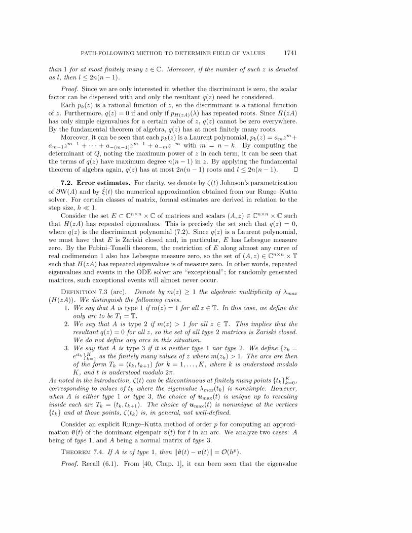
7.2. Error estimates. For clarity, we denote by \zeta (t) Johnson's parametrization

of \partial W(A) and by \^\xi (t) the numerical approximation obtained from our Runge--Kuttasolver. For certain classes of matrix, formal estimates are derived in relation to thestep size, h \ll 1.

Consider the set E \subset \BbbC n\times n \times \BbbC of matrices and scalars (A, z) \in \BbbC n\times n \times \BbbC suchthat H(zA) has repeated eigenvalues. This is precisely the set such that q(z) = 0,where q(z) is the discriminant polynomial (7.2). Since q(z) is a Laurent polynomial,we must have that E is Zariski closed and, in particular, E has Lebesgue measurezero. By the Fubini--Tonelli theorem, the restriction of E along almost any curve ofreal codimension 1 also has Lebesgue measure zero, so the set of (A, z) \in \BbbC n\times n \times \BbbT such thatH(zA) has repeated eigenvalues is of measure zero. In other words, repeatedeigenvalues and events in the ODE solver are ``exceptional""; for randomly generatedmatrices, such exceptional events will almost never occur.

Definition 7.3 (arc). Denote by m(z) \geq 1 the algebraic multiplicity of \lambda max

(H(zA)). We distinguish the following cases.1. We say that A is type 1 if m(z) = 1 for all z \in \BbbT . In this case, we define the

only arc to be T1 = \BbbT .2. We say that A is type 2 if m(z) > 1 for all z \in \BbbT . This implies that the

resultant q(z) = 0 for all z, so the set of all type 2 matrices is Zariski closed.We do not define any arcs in this situation.

3. We say that A is type 3 if it is neither type 1 nor type 2. We define \{ zk =eitk\} Kk=1 as the finitely many values of z where m(zk) > 1. The arcs are thenof the form Tk = (tk, tk+1) for k = 1, . . . ,K, where k is understood moduloK, and t is understood modulo 2\pi .

As noted in the introduction, \zeta (t) can be discontinuous at finitely many points \{ tk\} Kk=0,corresponding to values of tk where the eigenvalue \lambda max(tk) is nonsimple. However,when A is either type 1 or type 3, the choice of \bfitu max(t) is unique up to rescalinginside each arc Tk = (tk, tk+1). The choice of \bfitu max(t) is nonunique at the vertices\{ tk\} and at those points, \zeta (tk) is, in general, not well-defined.

Consider an explicit Runge--Kutta method of order p for computing an approxi-mation \^\bfitv (t) of the dominant eigenpair \bfitv (t) for t in an arc. We analyze two cases: Abeing of type 1, and A being a normal matrix of type 3.

Theorem 7.4. If A is of type 1, then \| \^\bfitv (t) - \bfitv (t)\| = \scrO (hp).

Proof. Recall (6.1). From [40, Chap. 1], it can been seen that the eigenvalue

1742 S\'EBASTIEN LOISEL AND PETER MAXWELL

\lambda (t) and the eigenvector \bfitu (t) are both analytic functions of t. Denote by \eta 1(t) \leq \eta 2(t) \leq \cdot \cdot \cdot \leq \eta n(t) = \lambda (t) the eigenvalues of H(eitA) and by DA(t,\bfitu (t), \lambda (t)) theunitary transform of MA(e

it,\bfitu (t), \lambda (t)) as defined in Definition 6.2. Since, by as-sumption, \lambda (H(eitA)) is simple for all t, then \eta n - 1(t) < \eta n(t), and so the eigenvalueof MA(e

it,\bfitu (t), \lambda (t)) with the smallest magnitude is either \eta n - 1(t) - \eta n(t) if thatquantity is small or \pm 1 from the lower-right 2 \times 2 block of DA(t,\bfitu (t), \lambda (t)). Eitherway, since \eta n - 1(t) - \eta n(t) is nonzero for every eit \in \BbbT and since \BbbT is compact, itmust be that the modulus of the spectrum | \sigma (MA(e

it,\bfitv max(t), \lambda max(t)))| is uniformlybounded below on \BbbT and henceM - 1

A (eit,\bfitu (t), \lambda (t)) is smooth in a neighborhood of thesolution curve. From the standard theory of Runge--Kutta methods, e.g., TheoremII.3.4 in [22], we obtain the result.

We now show that when A is normal, and \partial W(A) is, therefore, a polygon, ouralgorithm computes \partial W(A) exactly with no error. We begin with a technical lemmawhich shows that Runge--Kutta integrators preserve invariant subspaces.

Lemma 7.5. Consider a Runge--Kutta solver with S stages, with Butcher tableauB, c and step size h; in other words,

\bfity (s) = F

\left( \bfitx (0) + h

s - 1\sum j=1

Bsj\bfity (j)

\right) for s = 1, . . . , S and \bfitx (1) = \bfitx (0) + h

S\sum k=1

ck\bfity (k).

Say there is a matrix V such that \bfitx \in spanV =\Rightarrow F (\bfitx ) \in spanV , where spanVdenotes the column space of V . Then, if the initial data \bfitx (0) is in the column span ofV , all subsequent iterates \bfitx (k) shall also be in the column space of V .

Proof. Clearly, \bfity (0) = F (\bfitx (0)) \in spanV , and hence, by induction, \bfity (1), . . . ,\bfity (S) \in spanV . Finally, \bfitx (1) is a linear combination of vectors in spanV .

Theorem 7.6. Assume that A is a normal matrix with distinct eigenvalues anddenote the solution generated by Algorithm 6.1 as \^\xi (t), the Runge--Kutta approxima-

tion of the Johnson function \zeta (t). Then, \^\xi (t) = \zeta (t) for all t \in \bigcup

k Tk, where Tk arethe arcs as defined in Definition 7.3, i.e., there is no error.

Proof. Due to the spectral theorem, Property 2.3 (c), Property 2.3 (h), and The-orem 3 from [26], without loss of generality we may assume that A = diag(a1, . . . , an)with a1, . . . , an \in \BbbC . Then, H(eitA) = diag(\Re [eita1], . . . ,\Re [eitan]), and so the differ-ential equation is \biggl[

\bfitu \prime (t)\lambda \prime (t)

\biggr] = P (t)Q(t)

\biggl[ \bfitu (t)\lambda (t)

\biggr] = F

\biggl( \biggl[ \bfitu (t)\lambda (t)

\biggr] \biggr) ,

where

P (t) :=

\left[ \Re [eita1] - \lambda (t) - u1(t)

. . ....

\Re [eitan - 1] - \lambda (t) - un - 1(t)\Re [eitan] - \lambda (t) - un(t)

- u1(t) . . . - un - 1(t) - un(t) 0

\right] - 1

and

Q(t) :=

\left[ i\Im [eita1]

. . .

i\Im [eitan]0

\right] .

PATH-FOLLOWING METHOD TO DETERMINE FIELD OF VALUES 1743

Clearly,

F

\left( 0...0\ast \ast

\right) =

\left( 0...0\ast \ast

\right) , hence V =

\left[ 0 0...

...0 01 00 1

\right] is an invariant subspace for F . As per Algorithm 6.1, the initial value is the domi-nant eigenpair of H(eitA)\bfitu (t) = \lambda (t)\bfitu (t) so that \lambda (t) = \Re [eitan] and hence \bfitu (t) =[ 0 . . . 0 1 ]\ast = \bfite (n). In particular, the initial point \bfitx (0) is in the column space of Vand hence, by Lemma 7.5, all the Runge--Kutta steps are in the column space of V .This means that \^\bfitu max(t) is some multiple of \bfitu max(t) = \bfite (n), and \^\xi (t) = \zeta (t).

7.3. Discussion. We have proven the accuracy of our algorithm in the followingcases:

\bullet Type 1 matrices such that \lambda max(H(zA)) has multiplicity 1 for all z \in \BbbT : ouralgorithm produces an approximation \^\xi (t) of \zeta (t) that has \scrO (hp) accuracy.

\bullet Type 2 matrices such that \lambda max(H(zA)) has multiplicity 2 or higher for allz \in \BbbC : our algorithm does not work for those matrices.

\bullet Type 3 matrices: if A is normal, then \^\xi (t) = \zeta (t) and the numerical solutionis exact. We were not able to analyze the nonnormal case when nonsimpleeigenvalues are present.

Another way of expressing the above is to state the amount of work required toobtain a solution to the accuracy of a specific tolerance, \sigma . An important componentof this required work is the number of times we must perform an eigenproblem solve.For type 1 matrices, we need \scrO (\sigma 1/p) Runge--Kutta steps and the solution of oneeigenproblem to produce initial conditions, while for normal matrices of type 3, weneed \scrO (1) steps of the Runge--Kutta solver and one eigenproblem solve per arc. EachRunge--Kutta step requires SI linear solves to compute the SI stages, plus a smallnumber of linear solves SL for event detection. Thus, for fixed S = SI + SL and inthe cases we have analyzed, we predict \scrO (nA(\sigma

1/pSTL + TE)) work, where nA is thenumber of arcs, TL is the running time of a linear solve, and TE is the running time ofan eigenproblem solve. It is assumed that TE > TL. In our numerical experiments, nA

was often quite small. By comparison, Johnson's algorithm, which solves an eigenvalueproblem at m values of t, requires \scrO (mTE) work. Since Johnson's algorithm hasaccuracy \scrO (m - 2), we arrive at the following running times:

\bullet Our algorithm: \scrO (nA(\sigma - 1/pSTL + TE)).

\bullet Johnson's algorithm: \scrO (\sigma - 1/2TE).As we can see, for small \sigma and when nA is not too large, our algorithm is many ordersof magnitude faster than Johnson's algorithm. Apart from the difference in order\sigma - 1/p versus \sigma - 1/2, there is another trade-off that becomes obvious. Our algorithmrequires many fewer eigenvalue solves, and in exchange we require some linear solves.This is especially appealing when A is a sparse matrix in very high dimensions, wheresparse linear solvers may run faster than eigenvalue solvers.

Our algorithm does not apply to type 2 matrices, but this did not have a negativeimpact for our numerical experiments. We were also not able to completely analyzenonnormal matrices of type 3 (when \lambda max(t) can be nonsimple). These limitationsto our analysis are to be expected: even for the problem of computing eigenvalues,state-of-the-art eigenvalue solvers fail for some matrices.

1744 S\'EBASTIEN LOISEL AND PETER MAXWELL

8. Numerical tests. To provide a practical characterization of the new algo-rithm performance, numerical tests were performed to measure the error-cost trade-offin comparison with the existing algorithms.

8.1. Methodology for numerical tests. The most straightforward method todraw a fair comparison for practical use is to execute each algorithm within a range ofparameters, record the runtime and error, and then compare the results. This ensuresthat what is measured is the trade-off between computational cost and error tolerancefor each algorithm or parameter set. We considered a randomly generated complexmatrix A of size n = 250 with \| A\| = 1 for the numerical tests.

In [26], Johnson estimates the error by calculating the area of the inner and outerboundaries which act as a lower and upper bound on the actual area; the differencecan provide a suitable error measure for the number of boundary points calculated.However, if testing to high-precision, it is desirable to adopt an alternative errormeasure. Instead of using an area estimate, we attempt to calculate a ``maximumdistance"" error between the exact boundary and the interpolant produced by eachalgorithm. In other words, we calculate the maximum over the minimum distancebetween all points on the exact field of values boundary and the candidate interpolant.

Let \^\gamma (\cdot ) denote any generic parametrized boundary approximation (the interpo-lated output from a provided candidate algorithm). For a given exact Johnson pointpk = \zeta (tk) on \partial W(A), we define the error for a candidate algorithm at point pk as

\epsilon (pk) := mint\| pk - \^\gamma (t)\| ,

and the error for K Johnson points, pk, k \in \{ 1, . . . ,K\} as

E(K) := maxk\in \{ 1,...,K\}

\epsilon (pk),

and we seek to estimate

E := limK\rightarrow \infty

E(K) = limK\rightarrow \infty

maxk\in \{ 1,...,K\}

mint\| pk - \^\gamma (t)\| .

So that a valid comparison can be made with the analysis in section 7, we donot include in our measurements the time taken to compute the interpolant for eachalgorithm. For Johnson's algorithm and our path-following algorithm, these are es-sentially \scrO (1) operations and are not interesting. For Uhlig's algorithm, matters areslightly more involved.

Using new notation for clarity, in Uhlig's algorithm, for each of the me compres-sion ellipses one must calculate le boundary points, say. At the end of the algorithm'sprocessing, a convex hull of the total mele points must be calculated (the results ofwhich can be piecewise linearly interpolated similar to Johnson's algorithm). Cal-culating points on the ellipse is very lightweight but calculating the convex hull is\scrO (mele logmele). Uhlig's algorithm as it stands also does not directly make use ofthe higher-order interpolation available from the ellipses.

With a view toward making our analysis clearer, we define an Uhlig-lite variant.Rather than calculating a set of boundary points from each ellipse, we instead onlyperform the eigensolves and matrix compressions. This is obviously always faster thanUhlig's full algorithm and so represents a lower bound on computational cost, i.e.,Uhlig's full algorithm is always worse. To calculate E(K), we calculate the minimumdistance from each candidate pk point to the nearest exact ellipse boundary (using aroot solver). The effect of this is to determine the best-case asymptotic performance

PATH-FOLLOWING METHOD TO DETERMINE FIELD OF VALUES 1745

of the matrix compression approach if perfect interpolation on the relevant ellipsecould be done at no computational cost.

The eigenproblem solves for Johnson's algorithm, Uhlig's algorithm, and Uhlig-lite, and the path-following algorithm use QR decomposition. The Braconnier--Highammethod is approximated by a version of Johnson's algorithm with MATLAB's eigs()implementation of Lanczos using the previous eigenvector for the new start vector(continuation). Many of the enhancements that Braconnier and Higham proposed foruse in Lanczos (e.g., selective reorthonormalization and restarts) have been incorpo-rated or improved upon by the ARPACK library that underpins MATLAB's eigs(),so we have implemented a modern version of Braconnier--Higham by combining John-son's algorithm with MATLAB's eigs() solver.

The candidate algorithms are as follows: the path-following algorithm, Johnson'salgorithm, Johnson's algorithm using Lanczos with continuation (as per Braconnier--Higham), Uhlig's algorithm, and the Uhlig-lite variant. For each algorithm, we ap-proximate E to near machine precision by taking a suitably large K, picking each pkrandomly distributed over the boundary, and calculating the associated \epsilon (pk) values.This E(K) will almost certainly not achieve the maximum E unless we are very luckyin our choice of pk. So we therefore pick the J \ll K largest \epsilon (pk) points labeling thempj , j \in \{ 1, . . . , J\} , choose a small arc around each pj , create new pk points along eacharc and add to the list so that K grows, and finally re-evaluate E(K) using these newpoints. This divide-and-conquer approach is repeated until successive E(K) estimatesconverge to within machine precision, i.e., it has converged to E.

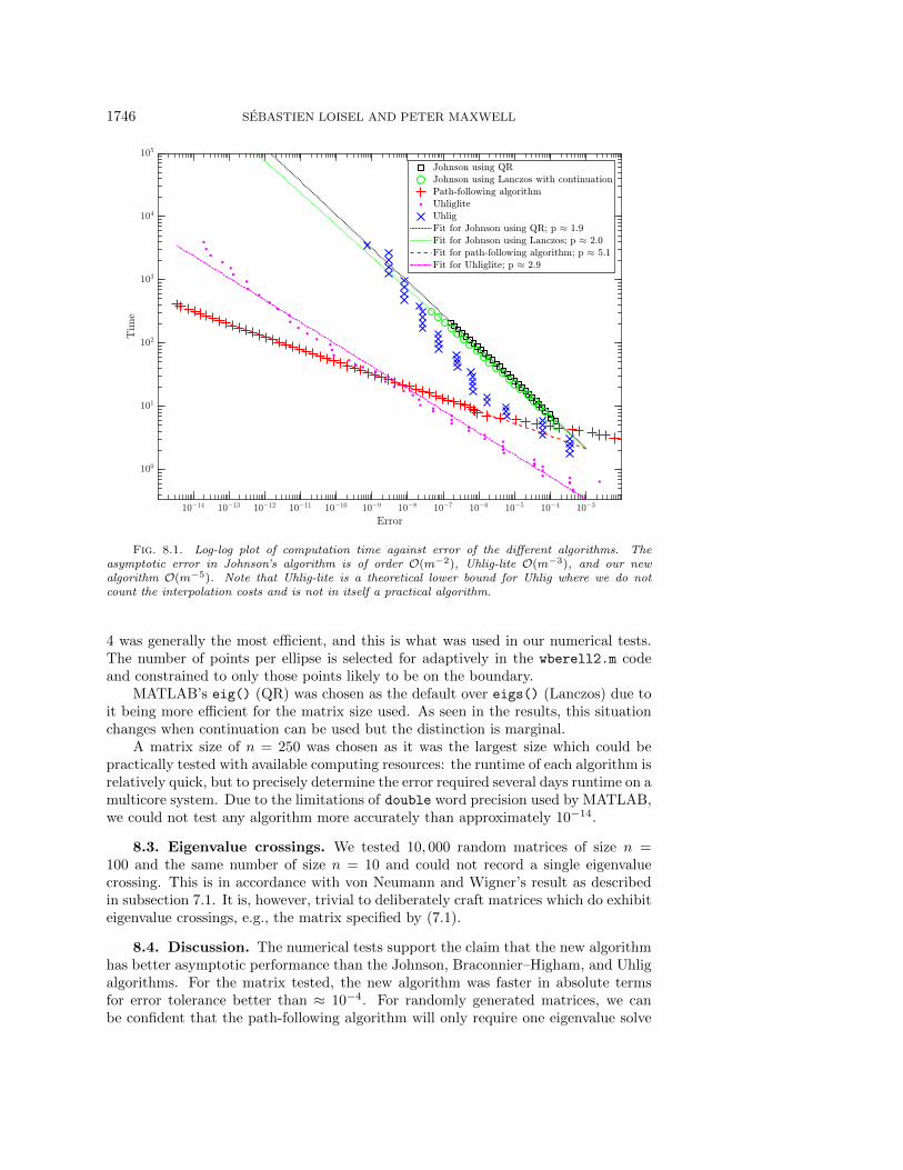
8.2. Numerical test results. The algorithms were tested for a reasonable rangeof parameters, e.g., for Johnson's algorithm we varied the number of eigensolves be-tween 28 and \approx 213. The parameter choices are not particularly important other thanforcing each algorithm to take longer to produce a more accurate result; it is theerror-cost relationship that we are interested in. The results are shown on a log-logplot in Figure 8.1. A linear fit has been applied so that the asymptotic complexity ofeach algorithm can be ascertained. This was not done for Uhlig's full algorithm.

Johnson and Johnson using Lanczos with continuation reduce error as predictedin [26], as \scrO (m - 2). Uhlig-lite reduces error approximately as \scrO (m - 3). The newalgorithm reduces error approximately as \scrO (m - 5). This is a significant improvementon existing algorithms in terms of asymptotic performance.

For the test matrix used, the path-following algorithm is faster in absolute termsthan all existing algorithms for accuracy better than around 10 - 4 (this excludes Uhlig-lite because it does not count the computation time for the ``exact"" interpolationused). Notably, the performance of Uhlig's algorithm deteriorates and becomes slowerthan Johnson's algorithm around 10 - 9 accuracy.

Although the asymptotic results should hold in general, some caution has to beadvised when attempting to draw conclusions about practical use cases. Factors suchas matrix size, matrix structure, regularity of \partial W(A), and CPU all have an influenceon the results. In particular, if a test matrix is structured such that computation oflinear solves are appreciably faster than eigenproblem solves, then the performance ofthe path-following algorithm improves significantly.

8.2.1. Additional details on test implementation. There are some per-tinent details concerning the implementation of the numerical tests which deservefurther explanation.

As mentioned in subsection 3.3, Uhlig described four methods [46, sect. 2.1] forselecting new edge-points. After tests using Uhlig's wberell2.m code [45], method

1746 S\'EBASTIEN LOISEL AND PETER MAXWELL

Fig. 8.1. Log-log plot of computation time against error of the different algorithms. Theasymptotic error in Johnson's algorithm is of order \scrO (m - 2), Uhlig-lite \scrO (m - 3), and our newalgorithm \scrO (m - 5). Note that Uhlig-lite is a theoretical lower bound for Uhlig where we do notcount the interpolation costs and is not in itself a practical algorithm.

4 was generally the most efficient, and this is what was used in our numerical tests.The number of points per ellipse is selected for adaptively in the wberell2.m codeand constrained to only those points likely to be on the boundary.

MATLAB's eig() (QR) was chosen as the default over eigs() (Lanczos) due toit being more efficient for the matrix size used. As seen in the results, this situationchanges when continuation can be used but the distinction is marginal.

A matrix size of n = 250 was chosen as it was the largest size which could bepractically tested with available computing resources: the runtime of each algorithm isrelatively quick, but to precisely determine the error required several days runtime on amulticore system. Due to the limitations of double word precision used by MATLAB,we could not test any algorithm more accurately than approximately 10 - 14.

8.3. Eigenvalue crossings. We tested 10, 000 random matrices of size n =100 and the same number of size n = 10 and could not record a single eigenvaluecrossing. This is in accordance with von Neumann and Wigner's result as describedin subsection 7.1. It is, however, trivial to deliberately craft matrices which do exhibiteigenvalue crossings, e.g., the matrix specified by (7.1).

8.4. Discussion. The numerical tests support the claim that the new algorithmhas better asymptotic performance than the Johnson, Braconnier--Higham, and Uhligalgorithms. For the matrix tested, the new algorithm was faster in absolute termsfor error tolerance better than \approx 10 - 4. For randomly generated matrices, we canbe confident that the path-following algorithm will only require one eigenvalue solve

PATH-FOLLOWING METHOD TO DETERMINE FIELD OF VALUES 1747

irrespective of the required accuracy. Given that this is the dominant factor in com-putational cost, the path-following algorithm should compare favorably to other al-gorithms which are heavily dependent on eigenvalue solves.

9. Conclusions and future work. We have presented a new algorithm forcalculating the field of values boundary for complex matrices. At high accuracy, ouralgorithm is at least an order of magnitude faster than all previous algorithms. Thereare open questions on finding optimal parameter sets and opportunities for furtheranalysis of nonnormal type 3 matrices which may form the subject of future efforts.

As mentioned in the introduction, we believe that the path-following algorithm wehave presented has more generic applicability. Indeed, one of the authors is currentlydeveloping a minor alteration of the algorithm for use in calculating dispersive proper-ties of ocean waves. As a result of this ongoing work, it appears our algorithm---withsuitable adjustments---has broad applicability for efficient solution of Sturm--Liouvilleproblems parametrized by a single real variable.

REFERENCES

[1] C. M. Bender and S. A. Orszag, Advanced Mathematical Methods for Scientists and Engi-neers I, Springer-Verlag, New York, 1999, https://doi.org/10.1007/978-1-4757-3069-2.

[2] W.-J. Beyn, C. Effenberger, and D. Kressner, Continuation of eigenvalues and invariantpairs for parameterized nonlinear eigenvalue problems, Numer. Math., 119 (2011), pp. 489--516, https://doi.org/10.1007/s00211-011-0392-1.

[3] W.-J. Beyn and V. Th\"ummler, Continuation of invariant subspaces for parameterizedquadratic eigenvalue problems, SIAM J. Matrix Anal. Appl., 31 (2010), pp. 1361--1381,https://doi.org/10.1137/080723107.

[4] T. Braconnier and N. J. Higham, Computing the field of values and pseudospectra using theLanczos method with continuation, BIT, 36 (1996), pp. 422--440, https://doi.org/10.1007/BF01731925.

[5] R. P. Brent, Algorithms for Minimization without Derivatives, Prentice Hall, EnglewoodCliffs, NJ, 1973.

[6] W. Cheney and D. Kincaid, Numerical Mathematics and Computing, Brooks/Cole, CengageLearning, Monterey, CA, 2012.

[7] M.-T. Chien and H. Nakazato, Flat portions on the boundary of the numerical ranges ofcertain Toeplitz matrices, Linear Multilinear Algebra, 56 (2008), pp. 143--162, https://doi.org/10.1080/03081080701217745.

[8] M.-T. Chien, L. Yeh, Y.-T. Yeh, and F.-Z. Lin, On geometric properties of the nu-merical range, Linear Algebra Appl., 274 (1998), pp. 389--410, https://doi.org/10.1016/S0024-3795(97)00373-X.

[9] H. Cohen, A Course in Computational Algebraic Number Theory, Springer-Verlag, Berlin,Heidelberg, 1993, https://doi.org/10.1007/978-3-662-02945-9.

[10] M. Crouzeix, Numerical range and functional calculus in Hilbert space, J. Funct. Anal., 244(2007), pp. 668--690, https://doi.org/10.1016/j.jfa.2006.10.013.

[11] C. Davis, The Toeplitz--Hausdorff theorem explained, Canad. Math. Bull., 14 (1971), pp. 245--246, https://doi.org/10.4153/CMB-1971-042-7.

[12] W. F. Donoghue, On the numerical range of a bounded operator, Michigan Math. J., 4 (1957),pp. 261--263, https://doi.org/10.1307/mmj/1028997958.

[13] J. R. Dormand and P. J. Prince, A family of embedded Runge--Kutta formulae, J. Comput.Appl. Math., 6 (1980), pp. 19--26, https://doi.org/10.1016/0771-050X(80)90013-3.

[14] P. F. Zachlin and M. E. Hochstenbach, On the numerical range of a matrix, Linear Multilin-ear Algebra, 56 (2008), pp. 185--225, https://doi.org/10.1080/03081080701553768, Englishtranslation with comments and corrections on a paper by Rudolph Kippenhahn.

[15] G. E. Forsythe, M. A. Malcolm, and C. B. Moler, Computer Methods for MathematicalComputations, Prentice Hall, Englewood Cliffs, NJ, 1977.

[16] I. M. Gelfand, M. Kapranov, and A. Zelevinsky, Discriminants, Resultants, and Multidi-mensional Determinants, 1st ed., Birkh\"auser Basel, Basel, 1994, https://doi.org/10.1007/978-0-8176-4771-1.

1748 S\'EBASTIEN LOISEL AND PETER MAXWELL

[17] N. Guglielmi and C. Lubich, Differential equations for roaming pseudospectra: Paths toextremal points and boundary tracking, SIAM J. Numer. Anal., 49 (2011), pp. 1194--1209,https://doi.org/10.1137/100817851.

[18] N. Guglielmi and C. Lubich, Erratum/Addendum: Differential equations for roaming pseu-dospectra: Paths to extremal points and boundary tracking, SIAM J. Numer. Anal., 50(2012), pp. 977--981, https://doi.org/10.1137/120861357.

[19] N. Guglielmi and M. L. Overton, Fast algorithms for the approximation of the pseudospectralabscissa and pseudospectral radius of a matrix, SIAM J. Matrix Anal. Appl., 32 (2011),pp. 1166--1192, https://doi.org/10.1137/100817048.

[20] K. Gustafson, The Toeplitz-Hausdorff theorem for linear operators, Proc. Amer. Math. Soc.,25 (1970), pp. 203--204, https://doi.org/10.1090/S0002-9939-1970-0262849-9.

[21] K. E. Gustafson and D. K. Rao, Numerical Range: The Field of Values of Linear Operatorsand Matrices, Springer, New York, 1997, https://doi.org/10.1007/978-1-4613-8498-4 1.

[22] E. Hairer, S. N{\e}rsett, and G. Wanner, Solving Ordinary Differential Equations I, Springer-Verlag, Berlin, Heidelberg, 1993, https://doi.org/10.1007/978-3-540-78862-1.

[23] F. Hausdorff, Der Wertvorrat einer Bilinearform, Math. Z., 3 (1918), pp. 314--316, https://doi.org/10.1007/BF01292610.

[24] R. A. Horn and C. R. Johnson, Topics in Matrix Analysis, Cambridge University Press,Cambridge, 1991, https://doi.org/10.1017/CBO9780511840371.

[25] C. R. Johnson, Normality and the numerical range, Linear Algebra Appl., 15 (1976), pp. 89--94, https://doi.org/10.1016/0024-3795(76)90080-X.

[26] C. R. Johnson, Numerical determination of the field of values of a general complex matrix,SIAM J. Numer. Anal., 15 (1978), pp. 595--602, https://doi.org/10.1137/0715039.

[27] T. Kato, A Short Introduction to Perturbation Theory for Linear Operators, Springer-Verlag,New York, 1982, https://doi.org/10.1007/978-1-4612-5700-4.

[28] R. Kippenhahn, \"Uber den Wertevorrat einer Matrix, Math. Nachr., 6 (1951), pp. 193--228,https://doi.org/10.1002/mana.19510060306.

[29] D. Kressner and B. Vandereycken, Subspace methods for computing the pseudospectralabscissa and the stability radius, SIAM J. Matrix Anal. Appl., 35 (2014), pp. 292--313,https://doi.org/10.1137/120869432.

[30] P. D. Lax, Linear Algebra and Its Applications, Pure Appl. Math., 2nd ed., John Wiley \&Sons Ltd, 2007, http://eu.wiley.com/WileyCDA/WileyTitle/productCd-0471751561.html.

[31] C.-K. Li, A simple proof of the elliptical range theorem, Proc. Amer. Math. Soc., 124 (1996),pp. 1985--1986, https://doi.org/10.1090/S0002-9939-96-03307-2.

[32] S. H. Lui, Computation of pseudospectra by continuation, SIAM J. Sci. Comput., 18 (1997),pp. 565--573, https://doi.org/10.1137/S1064827594276035.

[33] S. H. Lui, H. B. Keller, and T. W. C. Kwok, Homotopy method for the large, sparse, realnonsymmetric eigenvalue problem, SIAM J. Matrix Anal. Appl., 18 (1997), pp. 312--333,https://doi.org/10.1137/S0895479894273900.

[34] M. Marcus and C. Pesce, Computer generated numerical ranges and some resulting the-orems, Linear Multilinear Algebra, 20 (1987), pp. 121--157, https://doi.org/10.1080/03081088708817748.

[35] B. Moyls and M. Marcus, Field convexity of a square matrix, Proc. Amer. Math. Soc., 6(1955), pp. 981--983, https://doi.org/10.2307/2033121.

[36] F. D. Murnaghan, On the field of values of a square matrix, Proc. Natl. Acad. Sci. U.S.A.,18 (1932), pp. 246--248, http://www.pnas.org/content/18/3/246.full.pdf.

[37] P. J. Psarrakos and M. J. Tsatsomeros, Numerical range: (in) a matrix nutshell, Math-ematical Notes from Washington State University, v. 45 (2002) / v. 46 (2003), 2003,http://www.math.ntua.gr/\sim ppsarr/nutshell.ps.

[38] A. Quarteroni, R. Sacco, and F. Saleri, Numerical Mathematics, 2nd ed., Springer-Verlag,Berlin, Heidelberg, 2007, https://doi.org/10.1007/b98885.

[39] R. Raghavendran, Toeplitz--Hausdorff theorem on numerical ranges, Proc. Amer. Math. Soc.,20 (1969), pp. 284--285, https://doi.org/10.1090/S0002-9939-1969-0233186-5.

[40] F. Rellich, Perturbation Theory of Eigenvalue Problems, Gordon and Breach Science Pub-lishers, New York, London, Paris, 1969.

[41] L. F. Shampine, Some practical Runge--Kutta formulas, Math. Comp., 46 (1986), pp. 135--150,https://doi.org/10.2307/2008219.

[42] P. Sirkovi\'c and D. Kressner, Subspace acceleration for large-scale parameter-dependentHermitian eigenproblems, SIAM J. Matrix Anal. Appl., 37 (2016), pp. 695--718, https://doi.org/10.1137/15M1017181.

[43] T. Toeplitz, Das algebraische Analogon zu einem Satze von Fej\'er, Math. Z., 2 (1918), pp. 187--197, https://doi.org/10.1007/BF01212904.

PATH-FOLLOWING METHOD TO DETERMINE FIELD OF VALUES 1749

[44] L. N. Trefethen and M. Embree, Spectra and Pseudospectra: The Behavior of Nonnor-mal Matrices and Operators, Princeton University Press, 2005, http://press.princeton.edu/titles/8113.html.

[45] F. Uhlig, Source code from Frank Uhlig's webpage, http://www.auburn.edu/\sim uhligfd/m files/wberell2.m (retrieved Jan. 2017).

[46] F. Uhlig, Faster and more accurate computation of the field of values boundary for n by nmatrices, Linear Multilinear Algebra, 62 (2014), pp. 554--567, https://doi.org/10.1080/03081087.2013.779269.

[47] J. von Neumann and E. Wigner, On the Behavior of the Eigenvalues of Adiabatic Processes,World Scientific, pp. 25--31, https://doi.org/10.1142/9789812795762 0002.

[48] J. von Neumann and E. Wigner, \"Uber das Verhalten von Eigenwerten bei adiabatischenProzessen [On the behavior of the eigenvalues of adiabatic processes], in German, Physik.Z., 30 (1929), pp. 467--470.