Embed Size (px)
Citation preview
Path integral Monte Carlo study of one-dimensionalBose system: Luttinger liquid properties and impurityeffects
Lunić, Frane
Master's thesis / Diplomski rad
2017
Degree Grantor / Ustanova koja je dodijelila akademski / stručni stupanj: University of Split, University of Split, Faculty of science / Sveučilište u Splitu, Prirodoslovno-matematički fakultet
Permanent link / Trajna poveznica: https://urn.nsk.hr/urn:nbn:hr:166:202813
Rights / Prava: Attribution-ShareAlike 4.0 International
Download date / Datum preuzimanja: 2022-02-13
Repository / Repozitorij:
Repository of Faculty of Science
University of Split
Faculty of Science
Path integral Monte Carlo study ofone-dimensional Bose system:
Luttinger liquid properties and impurity effects
Master thesis
Frane Lunic
Split, September 2017
Temeljna dokumentacijska kartica
Sveucilište u Splitu Diplomski radPrirodoslovno – matematicki fakultetOdjel za fizikuRudera Boškovica 33, 21000 Split, Hrvatska
Istraživanje jednodimenzionalnih bozonskih sustava metodom integrala po stazama:osobine Luttingerove tekucine i utjecaj necistoca
Frane Lunic
Sveucilišni diplomski studij Fizika, smjer Racunarska fizika
Sažetak:Predstavljamo rezultate studije jednodimenzionalnih, uniformnih i neuredenih sustava interagirajucih
bozona, izvršene numerickom Monte Carlo metodom integrala po stazama (PIMC metoda). Interes za
ovu vrstu sustava je porastao nedavno otkad su eksperimentalno ostvareni u polju ultrahladnih atom-
skih plinova te adsorpcijom u uskim nanoporama. Nakon opisa teorijske pozadine i metoda predstavl-
jamo rezultate, fokusirajuci se na udio suprafluida, jednocesticnu matricu gustoce i korelacijsku funkciju
parova, te ih usporedujemo s predvidanjima teorije Luttingerove tekucine (LL). U slucaju uniformnih
sustava, pronalazimo slaganje te odredujemo Luttingerov parametarK na više nacina. Nakon dodavanja
necistoce na nasumicnom položaju u sustav, zaK < 1 nismo pronašli skaliranje udjela suprafluida s LT ,
što je vjerojatno znak lokalizacije predvidene u LL teoriji. Za K > 1 smo pronašli skaliranje što pred-
stavlja ocekivanu kvalitativnu razliku, ali rezultati pokazuju zanimljiva odstupanja od ocekivane relacije
skaliranja. U radu smo diskutirali moguca objašnjenja.
Kljucne rijeci: 1D, Luttingerova tekucina, nered, suprafluidnost, lokalizacija, kvantni Monte Carlo
Rad sadrži: 59 stranica, 20 slika, 0 tablica, 29 literaturnih navoda. Izvornik je na engleskom
jeziku.
Mentor: Dr. sc. Leandra Vranješ Markic, redoviti profesor Prirodoslovno-matematickog
fakulteta, Sveucilišta u Splitu
Ocjenjivaci: Dr. sc. Leandra Vranješ Markic, redoviti profesor Prirodoslovno-matematickog
fakulteta, Sveucilišta u Splitu
Dr. sc. Franjo Sokolic, redoviti profesor Prirodoslovno-matematickog fakulteta,
Sveucilišta u Splitu
Dr. sc. Petar Stipanovic, viši asistent Prirodoslovno-matematickog fakulteta,
Sveucilišta u Splitu
Rad prihvacen: 29. rujna. 2017.
Rad je pohranjen u Knjižnici Prirodoslovno – matematickog fakulteta, Sveucilišta u Splitu.
i
Basic documentation card
University of Split Master thesisFaculty of ScienceDepartment of PhysicsRudera Boškovica 33, 21000 Split, Croatia
Path integral Monte Carlo study of one-dimensional Bose system:Luttinger liquid properties and impurity effects
Frane Lunic
University graduate study programme Physics, orientation Computational Physics
Abstract:We present the results of a numerical path integral Monte Carlo (PIMC) study of one-dimensional uni-
form and disordered systems of interacting bosons. The interest in this kind of systems has grown
recently since they have been realized experimentally in the field of ultracold atomic gases, as well as
by adsorption of atoms in narrow nanopores. After providing theoretical background and laying out the
methods, we present the results, with focus on superfluid fraction, OBDM, and pair-correlation function,
and compare them with the predictions of the Luttinger liquid theory (LL). In case of uniform systems,
we find agreement. The Luttinger parameter K is determined in several ways. After adding a randomly
placed impurity to the system, for K < 1 we find no scaling of superfluid fraction with LT , most likely
signifying localization, as predicted by LL. Scaling is found for K > 1, indicating a qualitative differ-
ence, expected from LL. However, interesting deviations from the expected scaling relation are found.
Possible explanations are discussed.
Keywords: 1D, Luttinger liquid, disorder, superfluidity, localization, quantum Monte Carlo
Thesis consists of: 59 pages, 20 figures, 0 tables, 29 references. Original language: English.
Supervisor: Leandra Vranješ Markic, Ph.D., Professor at the Faculty of Science, University of
Split
Reviewers: Leandra Vranješ Markic, Ph.D., Professor at the Faculty of Science, University of
Split
Franjo Sokolic, Ph.D., Professor at the Faculty of Science, University of Split
Petar Stipanovic, Ph.D., Senior instructor at the Faculty of Science, University of
Split
Thesis accepted: September 29, 2017
Thesis is deposited in the library of the Faculty of Science, University of Split.
ii
Contents
1 Introduction 1
2 Theory 32.1 Theoretical background . . . . . . . . . . . . . . . . . . . . . . . . . . . . . . 3
2.1.1 Density matrix and quantum statistical mechanics . . . . . . . . . . . . 32.1.2 Bose-Einstein condensation . . . . . . . . . . . . . . . . . . . . . . . . 62.1.3 Superfluidity . . . . . . . . . . . . . . . . . . . . . . . . . . . . . . . 9
2.2 Path integral formalism . . . . . . . . . . . . . . . . . . . . . . . . . . . . . . 112.2.1 Path integral formulation of quantum mechanics . . . . . . . . . . . . . 112.2.2 Path integrals in quantum statistical mechanics . . . . . . . . . . . . . 142.2.3 Path winding and superfluidity . . . . . . . . . . . . . . . . . . . . . . 18
2.3 One-dimensional systems . . . . . . . . . . . . . . . . . . . . . . . . . . . . . 202.3.1 Theory of Luttinger liquids . . . . . . . . . . . . . . . . . . . . . . . . 21
3 Methods 253.1 Physical model and the basic simulation procedure . . . . . . . . . . . . . . . 253.2 Path integral Monte Carlo . . . . . . . . . . . . . . . . . . . . . . . . . . . . . 27
3.2.1 Metropolis algorithm and path integral Monte Carlo . . . . . . . . . . . 273.2.2 The problem of sampling in PIMC . . . . . . . . . . . . . . . . . . . . 293.2.3 Worm algorithm . . . . . . . . . . . . . . . . . . . . . . . . . . . . . . 303.2.4 Action approximation . . . . . . . . . . . . . . . . . . . . . . . . . . . 35
4 Results 364.1 The Luttinger parameter . . . . . . . . . . . . . . . . . . . . . . . . . . . . . . 36
4.1.1 The pair correlation function . . . . . . . . . . . . . . . . . . . . . . . 364.1.2 The structure factor . . . . . . . . . . . . . . . . . . . . . . . . . . . . 414.1.3 The one body density matrix . . . . . . . . . . . . . . . . . . . . . . . 444.1.4 Summary . . . . . . . . . . . . . . . . . . . . . . . . . . . . . . . . . 45
4.2 The superfluid fraction . . . . . . . . . . . . . . . . . . . . . . . . . . . . . . 464.2.1 Systems without disorder . . . . . . . . . . . . . . . . . . . . . . . . . 464.2.2 Systems with disorder . . . . . . . . . . . . . . . . . . . . . . . . . . . 48
5 Discussion 51
iii
5.1 Agreement with LL model for systems without disorder . . . . . . . . . . . . . 515.2 Classification of systems without disorder . . . . . . . . . . . . . . . . . . . . 525.3 Agreement with the LL prediction for disordered systems . . . . . . . . . . . . 53
6 Conclusion 55
iv
Chapter 1
Introduction
The topic of this thesis is exploration of properties of certain one-dimensional systems obeyingBose statistics. We touch upon many concepts of interest in condensed matter and ultra-cold gasphysics, such as superfluidity, Bose-Einstein condensation and the Tomonaga-Luttinger theoryof one-dimensional systems.
One-dimensional systems are not necessarily only toy models, and they can be fundamentallydifferent from, and no less difficult to understand than higher-dimensional systems, as theorieshighly successful in three dimensions tend to fail in one [9]. The difference is clearly visiblefrom the fact that perturbations can only give rise to collective excitations since there is noway for particles to move around each other. The Tomonaga-Luttinger liquid theory is a low-energy one-dimensional theory that successfully describes the physics of various simple one-dimensional systems [9]. It has been experimentally realised in cold atomic and other systems[25].
Aside from purely theoretical interest, the motivation for studying low-dimensional systemsstems from the possibility of their realization in various conditions. An example of this is thedesign of materials in such manner that movement of electrons becomes restricted in one ormore directions, which can result in quantization effects that preclude motion in the restricteddimensions [25]. In fact, most of the early research of one-dimensional systems was concernedwith electrons, since the study of electronic properties of quasi one-dimensional materials hasa clear potential for application. However, the distinction between Bose and Fermi systemsis not always clear cut. Cooper pairs behave to an extent as bosons [19], and the nature ofone-dimensional systems prevents the exchange of particles without collision, which reducesthe distinction between Bose and Fermi statistics [11]. The considerable overlap between re-sults on Bose and Fermi systems is part of the motivation for studying one-dimensional Bosesystems, and the relatively recent experimental developments have encouraged more theoreticalactivity in this field. These developments include confinement of cold atoms in essentially one-dimensional anisotropic traps, optical lattices, and elongated pores [19]. The properties of these
1
Frane Lunic: Luttinger liquid properties of 1D Bose system and impurity effects
systems can be modified by changing experimental conditions. For example, a uniform mag-netic field can be applied to control interactions via Feshbach resonances and optical latticescan be used to test theories of condensed matter physics [7].
Disordered systems are a topic of much interest in condensed matter physics, since latticeimperfections and impurities are almost inescapable, and give rise to phenomena such as resis-tivity. It has been shown that disorder can have a profound effect on conductive or superfluidproperties of one-dimensional systems. It causes localization of eigenstates in noninteractingsystems and the competition between superfluidity and localization in normally superfluid sys-tems [18, 19, 25]. Localization in presence of disorder has been confirmed numerically andexperimentally [25], but details are still a topic of research. The results on the effect of disorderon superfluidity of a recent numerical study of 4He atoms in narrow pores [17] show signs of lo-calization, but only when extrapolated to system sizes larger than those simulated, and apparentdisagreement with the prediction on the domain of validity of the Tomonaga-Luttinger liquidregime (see [19, 22]). It is our primary aim to further research this aspect, and we present herethe results and discussion of a similar study on disorder and superfluidity, the main differencebeing that simulations are performed in pure one-dimensional instead of quasi one-dimensionalgeometry.
This thesis is organized as follows. In chapter 2 we give a brief and cursory overview of therelevant physical theory. First we discuss topics of quantum statistical mechanics, Bose-Einsteincondensation, and superfluidity. Then we present the path integral formalism in quantum me-chanics, and its application to quantum statistical mechanics, along with derivation of the rela-tion between superfluidity and imaginary-time path winding around the periodic boundaries ofthe system. We conclude this chapter with discussion of one-dimensional quantum systems. Inchapter 3 we present the specifics of the simulated systems and outline the procedure followed,after which we discuss some of the general aspects of the path integral Monte Carlo method,and some of the more specific aspects of the worm algorithm implementation that we have used.Following this, in chapter 4 we present the obtained results on correlation functions and frac-tions of superfluid in systems with and without disorder. The results are further discussed inchapter 5, and final summary of conclusions is given in chapter 6.
2
Chapter 2
Theory
In this chapter we present the theory behind the studied phenomena and methods used in thestudy. We begin by covering some theory in the background of the more directly relevantone-dimensional theory. This includes the Bose-Einstein condensation and superfluidity, phe-nomena of interest to both physics of ultra-cold gases, and condensed matter physics. The pathintegral formalism, which is of interest to many branches of physics, is also introduced. We willassume particles are spinless throughout this chapter, and the remainder of this thesis.
2.1 Theoretical background
2.1.1 Density matrix and quantum statistical mechanics
Suppose a system is in a pure quantum state |φ〉. The projection operator is defined as |φ〉〈φ|,and its expectation value in the state |ψ〉 is the probability of a measurement yielding the state|ψ〉. This probability depends on the overlap of the two states, hence the projection of one ontoanother. Suppose now our system is a statistical mixture of states (a mixed state), that is, it canoccupy any of the states |φi〉 with probabilities given by pi.1 We may generalize the projectionoperator in the following manner.Let the set of |φi〉 be a complete set of orthonormal vectors.We define the density matrix as [1]
ρ =∑i
pi |φi〉〈φi| . (2.1)
1This is different from quantum superposition. A pure state can be a superposition of multiple states, but amixed state is not a superposition of pure states. Mixed states arise as a consequence of the uncertainty due tointeraction with the environment.
3

Frane Lunic: Luttinger liquid properties of 1D Bose system and impurity effects
If all probabilities are zero except for pj = 1, the pure state and the simple projection operatorare recovered. 2
If 〈φi|O|φi〉 is the expectation value of the operator O in the state φi, the mixed state expec-tation value is given by
〈O〉 =∑i
pi 〈φi|O|φi〉 . (2.2)
It can be shown by inserting the unit operator∑
j |φj〉〈φj| to the right of O in (2.2) and usingcommutative and distributive properties that
〈O〉 =∑j
〈φj|ρO|φj〉 ≡ Tr ρO. (2.3)
Let the system be composed of N particles, and let R = {r1, r2, ..., rN} represent a config-uration of the system’s coordinates. The density matrix elements in coordinate representationare given as
ρ(R,R′) = 〈R|ρ|R′〉 =∑i
pi φi(R)φ∗i (R′), (2.4)
where |R〉 and |R′〉 are states of different definite configurations of coordinates, and〈R|φi〉 = φi(R). The diagonal element ρ(R,R) ≡ ρ(R) is the probability of finding thesystem in the configurationR. The expectation value in the coordinate representation is
〈O〉 = Tr ρO =
∫dR 〈R|ρO|R〉 . (2.5)
By inserting the unit operator∫
dR′ |R′〉〈R′| between the two operators on the right hand sideof (2.5) we obtain the expression [1, 3]
〈O〉 =
∫dR dR′ ρ(R,R′) 〈R′|O|R〉 (2.6)
We can now introduce the reduced p-body density matrices by integrating out coordinatesri>p and multiplying with the normalization factor N !
(N−p)! .3 The reduced density matrices can
be used to calculate expectation values of p-body operators (e.g. the two body potential) in amanner analogous to (2.6). The one-body density matrix (OBDM)
ρ(r, r′) = N
∫dr2 · · · drN ρ({r1, r2, ..., rN}, {r′1, r2, ..., rN}) (2.7)
is of the most interest for this thesis. By setting r = r′, we obtain the particle density
2It can be shown that the necessary and sufficient condition for a pure state is that the density matrix is idem-potent, meaning ρ2 = ρ.
3The particular normalization is convenient in the second quantization framework, but there are multiple nor-malization conventions as laid out in [4].
4

Frane Lunic: Luttinger liquid properties of 1D Bose system and impurity effects
n(r) ≡ ρ(r, r) .
Suppose the system of interest is in equilibrium with a heat bath, kept at a fixed temperature,volume and number of particles (the canonical ensemble), and let H be the Hamiltonian of thesystem. The probability of a microstate |φi〉 associated with the energy eigenvalue Ei is
pi =e−βEi
Z, (2.8)
Z being the partition function
Z =∑i
e−βEi = Tr e−βH . (2.9)
Now the density matrix takes the form
ρ =1
Z
∑i
e−βEi |φi〉〈φi| =e−βH
Z
∑i
|φi〉〈φi| , (2.10)
and finally [1, 3]
ρ =e−βH
Z. (2.11)
In this case, it is useful to denote the density matrix with β, as in ρ(R,R′; β).
It can be shown by differentiating an element ρij = δije−βEi of the density matrix (2.11) that
ρ(β) satisfies the equation
− ∂ρ(β)
∂β= Hρ. (2.12)
In case of a one-dimensional particle, (2.12) is a simple diffusion equation
− ∂ρ(x, x′; β)
∂β= −λ ∂
2
∂x2ρ(x, x′; β), (2.13)
where λ = ~22m
. The initial condition can be chosen as ρ(x, x′; 0) = δ(x−x′) 4, and the solutionis given by
ρ(x, x′; β) = (4πλβ)−1/2 exp
[−(x− x′)2
4λβ
](2.14)
Generalizing to N three-dimensional particles, we have
ρ(R,R′; β) = (4πλβ)−3N/2 exp
[−(R−R′)2
4λβ
]. (2.15)
This equation can be applied to the case of particles in a box, as long as thermal wavelength
4This corresponds to perfect localization of the particle at infinite kinetic energy, and therefore, zero de Brogliewavelength.
5
Frane Lunic: Luttinger liquid properties of 1D Bose system and impurity effects
ΛT =√
2βλ is much less than the size of the box [3].
Symmetrized density matrix
So far, we have dealt only with distinguishable particles. More realistic systems of indistin-guishable particles can only occupy states that are either symmetric or antisymmetric with re-spect to the exchange of particles.
Let P be a permutation of particle labels, so that PR = {rP1 , rP2 , . . . , rPN}. We haveφ±(PR) = (±1)sgnPφ(R), where the index + denotes the symmetric, and - antisymmetricstate. Let us define symmetrization and antisymmetrization operators by
P± φ(R) =1
N !
∑P
(±1)sgnPφ(PR). (2.16)
It can be shown from group theory that when the operators act on an arbitrary state they projectout (anti)symmetric states [1, 3]. This allows us to construct Bose or Fermi density matrix fromthe density matrix of distinguishable particles (2.4),
ρ±(R,R′; β) ≡ P± ρD(R,R′; β)) =1
N !
∑P
(±1)sgnPρD(R,PR′; β). (2.17)
Since we are interested in Bose systems, we will denote P ≡ P+, and write the Bose densitymatix
ρB(R,R′; β) =1
N !
∑P
ρD(R,PR′; β). (2.18)
2.1.2 Bose-Einstein condensation
Bose-Einstein condensate is a state of matter in which the lowest energy level is macroscopicallyoccupied, meaning the number of particles in the lowest level is of the order of the total numberof particles N . This phenomenon does not occur in fermionic systems due to Pauli exclusionprinciple. We will show how this occurs in a uniform gas of non-interacting bosons.
The total number of particles must equal the sum of average occupation numbers of single-particle states, given by the Bose-Einstein (BE) distribution
N =∑i
ni =∑i
1
eβ(εi−µ) − 1, (2.19)
εi being the energy of the state i, and µ the chemical potential. Normally, if N is large, and kBTis much greater than the difference in energy between levels, one can replace the sum in (2.19)
6
Frane Lunic: Luttinger liquid properties of 1D Bose system and impurity effects
by an integral
N ≈ NT =
∫dε g(ε)
1
eβ(εi−µ) − 1, (2.20)
where g(ε) is the density of states, and NT is the number of excited particles, the thermal com-ponent of the system. We can equate the thermal component with the total number of particlesbecause each state, including the ground state, is only microscopically occupied. However, ifthe ground state becomes macroscopically occupied it will not be accounted for in (2.20).
Due to the subtraction in the denominator of the BE distribution, and the fact that occupancynumbers can not be less than zero, there is a constraint on the chemical potential, namely µ ≤ ε0.It’s value is fixed by the normalization condition
N = N0 +NT . (2.21)
Bose-Einstein condensation (BEC) occurs in the limit µ→ ε0, as the number of particles in theground state N0 ≡ n0 = {exp[β(ε0 − µ)]− 1}−1 diverges. Certain conditions must be met inorder for the transition to occur. The thermal component NT is an increasing function of µ at aconstant temperature. If its peak Nc(T ) = NT (T, µ = ε) is greater than N , the system can notcondense at that temperature. However, Nc(T ) decreases as temperature is lowered, and theremay exist a temperature Tc at which it becomes equal to N . Below Tc, N0 = N −NT is of theorder of N , and µ → ε0 in the thermodynamic limit. To determine the critical temperature, wefind the highest temperature at which N0 is macroscopic by setting
NT (Tc, µ = ε0) = N (2.22)
The density of states for a variety of systems is of the form [7]
g(ε) = Cpεp−1. (2.23)
In case of a gas of free particles, p = d/2, where d is the dimensionality of the system. In athree dimensional system, we have a square-root dependence on energy, and C3/2 = V m3/2
21/2π2~3 .The ground-state has zero energy, so µ is always negative. Inserting (2.23) into (2.20)
NT = Cp(kBT )p Γ(p) gp(eβµ), (2.24)
where
gp(z) =1
Γ(p)
∞∫0
dxxp−1
z−1ex − 1=∞∑l=1
zl
lp. (2.25)
7

Frane Lunic: Luttinger liquid properties of 1D Bose system and impurity effects
Now we set µ = 1, and insert (2.24) into (2.22) and obtain
kBTc =
[N
CpΓ(p)gp(1)
]1/p
. (2.26)
Inserting g3/2(1) = 2.612 for three-dimensional ideal gas, we have kBT ≈ 3.31~2n2/3
m, where
n = N/V is the number density. On the other hand, for p ≤ 1, gp(1) is divergent. It turns outthat for p = 1 the equation (2.26) holds for Tc = 0, so in two dimensions, BEC occurs at zerotemperature5, but for p < 1, BEC does not occur at all.
Next we demonstrate the existence of off-diagonal long-range in the OBDM of a Bose-condensed system. We may write the momentum distribution as
n(p) =⟨Ψ†(p)Ψ(p)
⟩. (2.27)
Since Ψ(p) = (2π~)−3/2 ∫ dr exp(ip · r/~)Ψ(r), we have
n(p) =1
(2π~)3
∫dr dr′ n(r, r′)eip·(r−r
′)/~ (2.28)
Assuming a uniform and isotropic system in a volume V, n(r, r′) = n(s = |r − r′|), and wecan write
n(s) =1
V
∫dpn(p)e−ip·s/~. (2.29)
If n(p) is a smooth function, the rapid oscillation of the exponential factor for large s will bringthe OBDM to zero when s → ∞. However, in presence of BEC, the momentum distributionhas an N0δ(p) term, and this causes the OBDM to approach a finite value n0 = N/V for larges. This is referred to as the off-diagonal long-range order.
We will now identify the order parameter of the BEC transition starting with the field operatorwritten in the form
Ψ(r) = φ0(r)a0 +∑i 6=0
φi(r)ai, (2.30)
φi(r) and ai being respectively the one-particle wave function and the annihilation operatorcorresponding to the i-th eigenstate of the OBDM. Since 〈a†0a0〉 = N0 � [a0, a
†0] = 1, we may
replace the ladder operator in the first term on the right-hand side of (2.30) with√N0. This way
we treat the first, macroscopic term as a classical field Ψ0(r), referred to as the wave function,and serving as the order parameter. This is called the Bogoliubov approximation. We may writeΨ0 in terms of its modulus and phase
Ψ0(r) = |Ψ0(r))| eiS(r). (2.31)
5Note that this result is not valid for two-dimensional systems in general. For example, p = 2 in a harmonictrap, and Tc is finite.
8
Frane Lunic: Luttinger liquid properties of 1D Bose system and impurity effects
The time dependent order parameter can be defined as
Ψ0(r, t) = Ψ0(r)e−iµt/~. (2.32)
The time dependence is governed by the chemical potential because Ψ0 can be thought of asthe matrix element of Ψ between the ground states with N and N + 1 particles, giving rise tothe EN+1 − EN ≈ ∂E
∂N= µ in the exponent [6, 7].
2.1.3 Superfluidity
Here we will describe the Landau’s criterion for superfluidity. Essentially, the criterion is basedon the possibility of energy dissipation through creation of energetically favourable elementaryexcitations in a fluid moving through a capillary.
First, we write the transformation laws of energy and momentum under Galilean transforma-tions [6]
E ′ = E − P · V +1
2MV 2, (2.33)
P ′ = P −MV , (2.34)
whereM is the total mass of the fluid, E andP are the energy and the momentum of the fluid ina reference frame K, and their primed counterparts are the energy and momentum in a differentframe K ′, moving with velocity V relative to K.
Suppose an excitation with momentum p appears in a zero temperature uniform fluid flowingthrough a capillary at a constant velocity v. The energy in the reference frame moving withthe fluid is raised from ground state E0 to E0 + ε(p), ε(p) being the energy of the excitation,while the momentum becomes p. According to (2.33) and (2.34), in the reference frame of thecapillary, the energy and momentum are given by
E ′ = E0 + ε(p) + p · v +1
2Mv2 (2.35)
P ′ = p+Mv. (2.36)
The energy of the elementary excitation of momentum p in the frame moving with the capillaryis given by ε(p) + p · v. In order for excitations to spontaneously arise on account of relativemotion, they have to reduce the total energy of the fluid from the perspective of the capillary,and therefore
ε(p) + p · v < 0 (2.37)
must hold. For momentum p, this is possible if v > ε(p)/p. We define the critical velocity vcas the smallest velocity such that (2.37) can hold for any p. Below vc, the fluid is stable against
9
Frane Lunic: Luttinger liquid properties of 1D Bose system and impurity effects
dissipation of its kinetic energy. Thus, the Landau’s criterion for superfluidity is
v < vc = minp
ε(p)
p. (2.38)
It depends on the shape of the excitation spectrum whether a system can achieve superfluidity,e.g. for the ideal Bose gas ε(p) = p2
2mleads to vc = 0, while the weakly-interacting Bose gas,
and even strongly-interacting 4He have a finite vc [6].
At a finite temperature, small compared to the critical temperature for superfluidity, we mayassume that our system is a gas of non-interacting quasiparticles corresponding to elementaryexcitations6. These quasiparticles can collide with the walls and exchange energy and momen-tum, but they only transport a part of the total mass, and the rest of the mass behaves like asuperfluid. Therefore the system has superfluid and normal fluid components, and each has itsown velocity, vs and vn respectively. In order for superfluidity to be possible, |vs − vn| < vc
must hold. In equilibrium, the normal component must be at rest with respect to the capillary,therefore vn = 0 in the frame of the capillary, and the relative velocity between the superfluidcomponent, and the capillary is vs − vn. Now, we can use the energy of the excitation in thecapillary frame to write the BE distribution function of quasiparticles
Np =1
exp{β [ε(p) + p · (vs − vn)]} − 1. (2.39)
It is of interest to determine the fraction of the system belonging to the superfluid component.As is shown in [6], the mass density of the normal component is given to the first order in vs−vnby the Landau formula
ρn = −1
3
∫dNp
dε
∣∣∣∣vs−vn=0
(ε) p2 dp
(2π~)3. (2.40)
The superfluid fraction can then be obtained from ρsρ
= 1 − ρnρ
. However, this theory is oflimited applicability, since we have assumed, as mentioned, a uniform fluid at a low enoughtemperature, and well-defined, non-interacting elementary excitations.
A connection can be established between BEC and superfluidity by identifying the currentdensity of the condensate with n0vs, where n0 = |Ψ0|2 is the number density of the conden-sate7[6, 8]. The system is assumed here to be uniform, and vs to be constant (or varying slowlyenough). The current density is given by
j =i~2m
(Ψ0∇Ψ∗0 −Ψ∗0∇Ψ0) =~mn0∇S. (2.41)
6This assumption is not always valid, e.g. in presence of disorder, elementary excitations are not well defined[6].
7However, it would be erroneous to assume that the density of the condensate is equal to the density of thesuperfluid.
10
Frane Lunic: Luttinger liquid properties of 1D Bose system and impurity effects
Therefore,
vs =~m∇S. (2.42)
The phase S is the velocity potential, and it follows that the flow of superfluid is irrotational.
It should be noted that the connection we have established does not apply in the most generalsense. Most notably, it breaks down in low dimensions. In two dimensions, irrotational super-flow can exist in absence of off-diagonal long-range order at temperatures above absolute zero[6]. However the decay of the OBDM is algebraic instead of exponential in this case, indicat-ing the existence of a quasi long-range order. Aside from this, superflow may be observed insystems of finite size, and as we will see, may be entirely a finite-size effect.
2.2 Path integral formalism
The path integral formalism, originating in the work of Richard P. Feynman, is a method thatcan be applied to study quantum systems. It is based on associating a probability amplitudewith a completely specified motion of the system, its path. The integral over all possible pathswithin a region of space-time leads to the probability amplitude of the system occupying thisregion.
The formalism can be applied in slightly different manners to formulation of either quantummechanics or quantum statistical mechanics. We will first briefly present the path integral for-mulation of quantum mechanics along the lines of Feynman’s 1948. aritcle [2]. We will thenturn to the path integral formulation of quantum statistical mechanics, which lays the theoreticalfoundation of the path integral Monte Carlo method.
2.2.1 Path integral formulation of quantum mechanics
This formulation of quantum mechanics rests on two postulates which we quote directly from[2]:
1. If an ideal measurement is performed to determine whether a particle has a path lying
in a region of space-time, then the probability that the result will be affirmative is the
absolute square of a sum of complex contributions, one from each path in the region.
2. The paths contribute equally in magnitude, but the phase of their contribution is the clas-
sical action (in units of ~) ; i.e., the time integral of the Lagrangian taken along the path.
We denote the space-time region of interest R. To understand what is meant by path lying inthis region, we can imagine splitting the motion of a particle moving in the direction x in alarge number of time slices ti, separated by a time interval ε. The positions of the particle at
11
Frane Lunic: Luttinger liquid properties of 1D Bose system and impurity effects
times ti are denoted xi. Letting ε → 0, the (xi, ti) pairs define the path x(t). Region R cannow be defined as a set of (ai, bi) pairs, and the paths lying in R satisfy ai < xi < bi. Wecan now understand the concept of "ideal measurement" as a hypothetical measurement suchthat no further information may be extracted from it without disturbing the system beyond thedisturbance of measuring weather the path lies in R. If a system was further disturbed, e.g. ifone of the xi’s was collapsed into a specific value, the calculation of probability would have tochange, since we would be dealing with classical probabilities instead of probability amplitudes.
The first postulate leads to the expression for probability amplitude of the path of the particlelying in a region R of space-time
ϕ(R) = limε→0
∫R
Φ(..., xi, xi+1, ...) · · · dxi dxi+1 · · · , (2.43)
where the notation∫R
stands for · · ·∫ biai
∫ bi+1
ai+1· · · , and Φ(..., xi, xi+1, ...) is the complex contri-
bution to the probability amplitude of a path defined by sequence of xi’s. As ε approaches zero,this essentially becomes a functional of path Φ[x(t)]. The second postulate implies
Φ[x(t)] ∝ ei~S[x(t)], (2.44)
S being the action, defined as the time integral of the classical Lagrangian along the path x(t)
S[x(t)] =∫L(x(t), x(t))dt. In order to pass (2.44) to (2.43), x(t) has to be defined in the
interval between ti and ti+1. This is done by assuming that the particle follows the classicalpath between ti and ti+1, that is the path of minimal action. We may write
S =∑i
S(xi+1, xi), (2.45)
and
S(xi+1, xi) = min
ti+1∫ti
L(x(t), x(t)) dt . (2.46)
Finally, we arrive at
ϕ(R) = limε→0
∫R
exp
[i
~∑i
S(xi+1, xi)
]∏i
dxiA, (2.47)
where∏
i 1/A is the normalization factor. This completes the path integral formulation ofquantum mechanics.
In order to prove the equivalence of this formulation with ordinary quantum mechanics, weshould be able to define the wave function, and show it obeys the Schrödinger’s equation (thisproof still neglects spin, however). We will cover this in a brief and somewhat crude manner,
12
Frane Lunic: Luttinger liquid properties of 1D Bose system and impurity effects
and the reader may wish to see the full derivations in [2], or skip to the next section.
First we divide R into regions R′ lying in the past, i.e. before some time t′ < t (t being thepresent), and R′′ in the future, i.e. after some time t′′ > t. The remaining region between t′ andt′′ can be arbitrarily narrow, and the values of the x coordinates are not restricted in this region.The value |ϕ(R′, R′′)|2, if normalized by |ϕ(R′)|, can be interpreted as the probability that ifthe system was in region R′ it will later be found in region R′′. We assign the index i = 0 to thepresent. The amplitude is given by
ϕ(R′, R′′) =
∫dx0
∫R′′
1
A
∞∏i=0
{exp
[i
~S(xi+1, xi)
]dxi+1
A
}∫R′
−1∏i=−∞
{exp
[i
~S(xi+1, xi)
]dxiA
}(2.48)
Integration over the past and future regions R′ and R′′ in (2.48) produces functions ψ(x0, t) andχ∗(x0, t) respectively
ϕ(R′, R′′) =
∫χ∗(x, t)ψ(x, t)dx. (2.49)
The function ψ(x, t) is dependent only on the past history of the system, and vice versa forχ∗(x, t). At time t, the entire information about the system is contained in ψ(x, t). Futureexperiments can not distinguish between different histories, as long as they result in the samewave function. Similar remarks apply to χ∗(x, t) so it represents the complex conjugate ofthe wave function of a possible future state. We can interpret the right-hand side of (2.49)as the transition amplitude between the two states, i.e. the probability amplitude of a futuremeasurement yielding the state χ if the system was prepared in state ψ.
A recursive relation, exact in the limit ε→ 0, follows from the definition of ψ(x, t)
ψ(x1, t+ ε) =
∫R
exp
[i
~S(x1, x0)
]ψ(x0, t)
dx0
A. (2.50)
If we assume the relation is exact to the first order in ε, the accumulated error over a finiteinterval of time T will be of the order of Tε, since the number of factors is T/ε, each carrying atmost an error of order ε2. Therefore the error will vanish in the limit ε→ 0. We limit ourselvesto a case of the Lagrangian being a quadratic function of velocities, without terms linear invelocity (i.e. the vector potential). The action can now be approximated as an integral over thepath of a free particle8
S(x, x− ξ) =mε
2
(ξ
ε
)2
− εV (x), (2.51)
8This is limited to rectangular coordinates
13
Frane Lunic: Luttinger liquid properties of 1D Bose system and impurity effects
where x = x1, ξ = x1 − x0, and V (x) is the potential. Inserting this into (2.50), expanding theleft-hand side to first order in ε, and ψ(x− ξ) to second order of ξ we obtain
ψ(x, t) + ε∂ψ
∂t(x, t) + ... =
= exp
[−iεV (x)
~
] ∫exp
(imξ2
2~ε
)[ψ(x, t)− ξ ∂ψ(x, t)
∂x+ξ2
2
∂2ψ(x, t)
∂x2− ...
]dξ
A.
(2.52)
The only significant contribution to the right-hand side comes from region near ξ = 0, sinceotherwise the exponential due to kinetic action oscillates rapidly compared to variation in ψwhen ε is small, and thus ensures cancellation. Upon integration, we find that agreement tozero order sets the value of A, and expanding the exponential due to potential action, we finallyobtain the Schrödinger’s equation for a particle in one dimension, accurate to the first order in ε
i~∂ψ
∂t= − ~2
2m
∂2ψ
∂x2+ V (x)ψ. (2.53)
2.2.2 Path integrals in quantum statistical mechanics
If we rewrite the inverse temperature β = u/~, the new variable u has the dimension of time,and will be referred to as "time" for reasons we hope will become clear soon. The densitymatrix now takes the form
ρ(u) = exp(−u~H). (2.54)
We note that we have switched to using an unnormalized form of the density matrix. We maybreak time up into M intervals of duration ε, and write
ρ(u = Mε) =[exp(− ε~H)]M
. (2.55)
If we write each of the factors i in (2.55) in the position representation ρ(Ri,Ri−1), integrateoverRi for all i 6= 0,M we come to the rule of convolution
ρ(RM ,R0;u) =
∫ρ(RM ,RM−1; ε)ρ(RM−1,RM−2; ε) · · · ρ(R1,R0; ε) dR1 · · · dRM−1 .
(2.56)Once again, when ε→ 0, we have a path integral [1]
ρ(RM ,R0;u) =
∫Φ[R(s)] DR(s), (2.57)
where DR(u) = limM→∞
∏M−1i=1
dRi
A.
In case of free particles, we simply insert (2.15) on the right-hand side of (2.56), and let
14

Frane Lunic: Luttinger liquid properties of 1D Bose system and impurity effects
DR(u) absorb the normalization constant9 to find
Φ[R(s)] = limε→0
exp
{− ~
4λ
M−1∑i=0
ε
(Ri+1 −Ri
ε
)2}
= exp
−1
~
u∫0
m
2
[R(s)
]2
ds
, (2.58)
where we can recognize the kinetic energy term in the integral.
Since particles in a potential V (R) become asymptotically free when ε is very small com-pared to the scale of significant variation of V , we can still use the density matrix of freeparticles (denoted ρ0) for perturbation expansion of ρ
ρ(R,R′; ε) = ρ0(R,R′; ε) + δρ(R,R′; ε), (2.59)
where [1]
δρ(R,R′; ε) ≈ −∫
dR′′ε∫
0
ρ0(R,R′′; ε− u)V (R′′)ρ0(R′′,R′;u)du
~. (2.60)
Due to small ε, the free density matrices are very localized, so the majority of contribution tothe integral comes from the region in the vicinity of both R, and R′ (the R and R′ have to beclose in order for the integral to have a significant value). V (R′′) can be taken to be constant inthis region, and now theR′′ integral is simply a convolution of density matrices, so we find
δρ(R,R′; ε) ≈ −∫
du
~V (R)ρ0(R,R′; ε) = − ε
~V (R)ρ0(R,R′; ε). (2.61)
When dealing with larger ε the more accurate [1, 3] symmetrized form ε2~ [V (R) + V (R′)] will
be used. Equation (2.59) now becomes
ρ(R,R′; ε) ≈ ρ0(R,R′; ε)
[1− V (R)
~ε
]≈(
4πλε
~
)−3N/2
exp
{−ε
[~4λ
(R−R′
ε
)2
+V (R)
~
]}. (2.62)
This amounts to the primitive approximation in which the commutator terms of the order higherthan ε are ignored in the Baker-Campbell-Hausdorff formula
exp
[− ε~
(T + V) +ε2
2~2[T , V ] + . . .
]= exp
(− ε~T)
exp(− ε~V). (2.63)
The primitive approximation becomes exact in the sense that the error does not accumulate
9This is done for mathematical convenience, and we will reintroduce the normalization when dealing withdiscrete paths.
15

Frane Lunic: Luttinger liquid properties of 1D Bose system and impurity effects
when ε→ 0[3]. Finally,
ρ(RM ,R0;u) =
∫exp
−1
~
u∫0
[m2R(s)
2+ V (R(s))
]ds
DR(s) (2.64)
Note the similarity between equations (2.62) and (2.51). If we define
Si ≡ S(Ri,Ri−1; ε) ≡ −~ ln[ρ(Ri,Ri−1; ε)], (2.65)
then Si = Ki + U i, where the kinetic action is
Ki =3N~
2ln
(4πλε
~
)+
~2
4λ
(Ri −Ri−1)2
ε, (2.66)
and the potential action is simply the difference between the total and kinetic action. In primitiveapproximation, the potential action is written
U i1 =
ε
2[V (Ri) + V (Ri−1)] , (2.67)
where we have used the more precise symmetrized form as noted earlier, and the index rep-resents the order of approximation in ε. We return now to the equation (2.56) and rewrite itas
ρ(RM ,R0;u) =
∫exp
[−1
~
M∑i=1
S(Ri,Ri−1; ε)
]M−1∏i=1
dRi (2.68)
Again, we see a striking similarity to an earlier result from path integral quantum mechanics,the probability amplitude of a path lying in space-time region R (2.47), and we can see howthe variable u ∝ T−1 plays a role similar to conventional time. However, the imaginary unit islacking in the exponent of (2.68). We can introduce it by switching to imaginary time t = u
i
and ε → iε [5]. For the sake of argument, we ignore the constant term on the right-hand sideof (2.66), letting it be absorbed by DR(s) as before. Then the two equations are identical inform, and it can readily be shown that the kinetic and potential parts of action have differentsigns, as it should be the case, since the action is conventionally defined as the time integral ofthe Lagrangian. Now the density matrix element in coordinate representation can be interpretedas the probability amplitude for a system of N particles to travel from R0 to RM in durationt = β
i~ of imaginary time [1]. The amplitude is obtained by summing up contributions from allpossible paths. This interpretation implies the possibility of numerical calculation of the densitymatrix by sampling random walks.
16

Frane Lunic: Luttinger liquid properties of 1D Bose system and impurity effects
Classical isomorphism
We will now discuss the isomorphism between quantum and certain classical statistical systems[3], and use this opportunity to introduce some terminology along the way. Expression (2.68) isalso equivalent in form to a configuration integral of a classical system at an inverse temperatureof τ = ε/~ = β/M , as can be seen by extracting ε from the action. It is important not toconfuse the temperature of the classical system with the temperature of the quantum systemdefined by β10. The system in question is composed of N chains of particles, referred to asbeads to avoid confusion with the physical particles. These chains are called polymers, andeach represents a path of a particle in imaginary time, or its world line. The m-th bead ineach polymer corresponds to one of the N particles at the discrete point in time um = mε. Avector Rm = {r1,m, ..., rN,m} will be referred to as the m-th time slice, since it contains theconfiguration of the system at the time um. A pair of successive time slices (Rm−1,Rm) is thelink m, and the action Sm, as defined in (2.65), is the action of the link m.
The action divided by ε plays the role of the potential energy. Examining this potential energyfunction, we see that the kinetic part of the action gives rise to the spring potential between thesuccessive beads of the same polymer, and the potential action plays the same role of potentialbetween different particles. Note that this results in a rather peculiar classical system in whichthe beads belonging to different polymers only interact if they are at the same time slice.
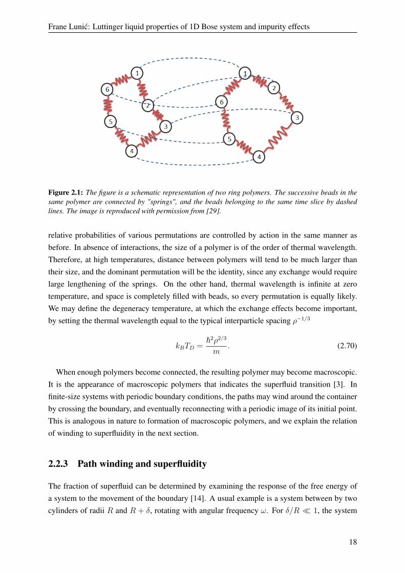
We are especially interested in diagonal elements of the density matrix ρ(R0,RM = R0). Infact, it makes sense to view the time u as periodic with period β~. Now the polymers becomering polymers. Due to quantum-classical isomorphism, any property that can be written in termsof the partition function, or even the density matrix elements, has an analogue in the statisticalmechanics of classical ring polymers [3]. Two ring polymers are schematically presented inFigure 2.1
Of course, the picture we have just presented only applies to distinguishable particles. As wehave seen earlier, the Bose density matrix and partition function must include a sum over allpossible permutations
ZB =1
N !
∑P
∫ρ(R0,PRM = R0; β) dR0 =
1
N !
∫exp
[−1
~
M∑m=1
Sm
]M−1∏m=0
dRm (2.69)
The boundary condition PRM = R0 implies that the polymers can become "cross-linked",since the polymer that contains the ri,0 bead can close onto rj,0, where j = Pi, after one timeperiod β. Since any permutation is a product of cyclic permutations, the chain will eventuallyclose onto ri,0 again. Multiple ring polymers are thus connected into one, and in presence ofnon-identity permutations, the number of rings is reduced by n − 1 for every n-cycle. The
10In fact, it makes sense in application to keep the time interval constant as quantum temperature is changed
17
Frane Lunic: Luttinger liquid properties of 1D Bose system and impurity effects
Figure 2.1: The figure is a schematic representation of two ring polymers. The successive beads in thesame polymer are connected by "springs", and the beads belonging to the same time slice by dashedlines. The image is reproduced with permission from [29].
relative probabilities of various permutations are controlled by action in the same manner asbefore. In absence of interactions, the size of a polymer is of the order of thermal wavelength.Therefore, at high temperatures, distance between polymers will tend to be much larger thantheir size, and the dominant permutation will be the identity, since any exchange would requirelarge lengthening of the springs. On the other hand, thermal wavelength is infinite at zerotemperature, and space is completely filled with beads, so every permutation is equally likely.We may define the degeneracy temperature, at which the exchange effects become important,by setting the thermal wavelength equal to the typical interparticle spacing ρ−1/3
kBTD =~2ρ2/3
m. (2.70)
When enough polymers become connected, the resulting polymer may become macroscopic.It is the appearance of macroscopic polymers that indicates the superfluid transition [3]. Infinite-size systems with periodic boundary conditions, the paths may wind around the containerby crossing the boundary, and eventually reconnecting with a periodic image of its initial point.This is analogous in nature to formation of macroscopic polymers, and we explain the relationof winding to superfluidity in the next section.
2.2.3 Path winding and superfluidity
The fraction of superfluid can be determined by examining the response of the free energy ofa system to the movement of the boundary [14]. A usual example is a system between by twocylinders of radii R and R + δ, rotating with angular frequency ω. For δ/R � 1, the system
18
Frane Lunic: Luttinger liquid properties of 1D Bose system and impurity effects
becomes essentially equivalent to a 2πR-periodic system enclosed by two planes moving withvelocity v = Rω. Here we study a more general system enclosed in a d-dimensional box,periodic in at least one direction, in a manner similar to [14].
Let ρv be the density matrix of a system with walls moving with an arbitrary velocity v.Since the distribution is identical in the lab and moving frame, we have ρv = ρ′ = e−βH
′ , whereprimed frame is at rest with the boundary, and
H ′ =N∑i=1
(−i~∇i −mv)2
2m+ V (R). (2.71)
We can define the normal component as the part which responds to the boundary motion. Thisimplies
ρnρNmv = 〈P 〉v =
Tr ρvP
Tr ρv, (2.72)
which we may rewrite as
ρnρNmv =
1
β∇v ln(Tr ρv) +Nmv. (2.73)
Since e−βFv = Tr ρv, and ρSρ
= 1− ρNρ
, by applying the chain rule we obtain
ρSρ
=∂Fv
∂(12mv2)
. (2.74)
Integrating form zero velocity to v, and expanding around constant fraction, we obtain the con-nection between the free energy response due to boundary motion and the fraction of superfluid
∆Fv
N=
1
2mv2 ρS
ρ+O(v4). (2.75)
As expected, due to dissipation, there is little impact of boundary motion on the bulk of thenormal fluid. However, the free energy response is proportional to the superfluid fraction.
From (2.12), we know that
− ∂ρv(R,R∗; β)
∂β= H ′ρv(R,R∗; β), (2.76)
with boundary condition
ρv(R, {r∗1, . . . , r∗j +L, . . . , r∗n}; β) = ρv(R,R∗; β). (2.77)
We can write
e−β∆Fv =
∫ρv(R,R; β) dR∫ρv=0(R,R; β) dR
, (2.78)
19
Frane Lunic: Luttinger liquid properties of 1D Bose system and impurity effects
where ρv=0 is the solution of the equation of motion for stationary walls. It can be shown byinserting in (2.76) that this equation is satisfied by ρ, defined by
ρv(R,R∗; β) = exp
[im
~v ·∑i
(ri − r∗i )
]ρ(R,R∗; β). (2.79)
Obviously, we have e−βFv=0 = Tr ρ, which is precisely the denominator of (2.78), but one thingremains to be clarified. SettingR∗ = R, the sum in the exponent of (2.79) takes the form∑
i
(rPi − ri) ≡W , (2.80)
where the winding vector W counts the number of times the paths wind around the box ineach direction. Its components Wα are quantized in units of Lα, the length of the box in the αdirection. If the path closes onto the k-th periodic image of the initial bead, then Wα = kLα.Now we may write
e−β∆Fv =
∫eim~ v·W ρ(R,R; β) dR∫ρ(R,R; β) dR
=⟨eim~ v·W ⟩ . (2.81)
Since velocity is arbitrary, we may take it to be small. All of the odd terms in the expansion ofei
~2λ
v·W average to zero, and we have
β∆Fv =m2
2~2〈(v ·W )2〉+O(v4) =
m2v2
2~2〈W 2〉+O(v4), (2.82)
where W = v|v| ·W is the winding number in the direction of v. If we take v = vxex for exam-
ple, it is the x component of the winding vector, and if our box is a d-dimensional hypercube, itbecomes obvious due to symmetry that 〈W 2〉 = 1
d〈W 2〉. By comparing (2.82) with (2.75), we
finally arrive at the expression for the superfluid fraction in terms of the mean square windingnumber, which can be calculated from the flux of paths across any plane
ρSρ
=〈W 2〉2λβN
. (2.83)
2.3 One-dimensional systems
Next, we turn to the theory of quantum one-dimensional systems. 1D systems are fundamen-tally different from their higher-dimensional counterparts which causes many of the methodsdeveloped for studying 3D systems to fail. Before moving on to the Luttinger liquid theory thatis of particular interest for this thesis, we will briefly mention some of the important results.Recall that BEC does not exist in 1D. This is due to the fact that fluctuations of the phase de-stroy long-range order. Even algebraic order is only present at zero temperature [6]. We will see
20

Frane Lunic: Luttinger liquid properties of 1D Bose system and impurity effects
that superflow can exist in 1D, but only in systems confined to small size, since imaginary-timepaths are still able to wind around the system in presence of periodic boundary conditions.
2.3.1 Theory of Luttinger liquids
The Tomonaga-Luttinger model is a theory developed for studying the low energy properties of1D systems of interacting fermions. We will use the term Luttinger liquid (LL) to refer to eitherthis model or any systems that share its low energy characteristics, which includes a variety of1D systems, not necessarily fermionic. The LL model is an analogue of the Fermi liquid modelwhich fails in 1D. The Fermi liquid is a generalization of the Fermi gas to systems of interactingfermions, and it preserves a lot of the properties of the Fermi gas, notably the discontinuity ofthe zero-temperature fermion distribution at the Fermi surface11, and the excitations that have aone-to-one correspondence to the free system. Near the Fermi surface, the excitations resembleparticle-hole pairs, but have a finite lifetime, which can nevertheless be considered infinitelylong for most practical purposes [9, 10].
The LL model describes the low lying excitations around the two Fermi points12. As longas we stay in the vicinity of Fermi points, the dispersion relation can be linearized, leading toHamiltonian [10]
H =∑α=±1
vF
∫dx Ψ†α(i~α∂x − ~kF )Ψα −
1
2
∫dx dx′ ρ(x)V (x− x′)ρ(x′), (2.84)
where α labels the Fermi points, and vF and ~kF are Fermi velocity and momentum. The± fields correspond to excitations moving in opposite directions, and the density is given byρ = Ψ†+Ψ+ + Ψ†−Ψ−. Various methods can be applied to this model, including perturbationtheory, renormalization groups, and bosonization. The last is of most interest to us since it isspecific to 1D, and makes obvious the connection to Bose systems in 1D.
Let us start from a Bose fluid of average density ρ0 = N0/L, and let Ψ(x) be an L-periodicfield satisfying the commutation relation
[Ψ(x), Ψ†(x′)] = δ(x− x′). (2.85)
The Hamiltonian of the fluid is given by
H =~2
2m
∫dx |∇Ψ|
2+
1
2
∫dx dx′ Ψ†(x)Ψ†(x′)V (x− x′)Ψ(x)Ψ(x′). (2.86)
11Note that the magnitude of the jump is decreased since the distribution is no longer a step function.12The analogue of the Fermi surface in 1D.
21

Frane Lunic: Luttinger liquid properties of 1D Bose system and impurity effects
We proceed by introducing the phase-density representation
Ψ†(x) =√ρ(x)eiϕ(x), (2.87)
where
ρ(x) =N∑n=1
δ(x− xn) (2.88)
is the density operator, and ϕ the phase operator. Then, assuming eiϕ commutes with itself forx 6= x′, it follows from commutator (2.85) that
[ρ(x), eiϕ(x′)] = eiϕ(x)δ(x− x′), (2.89)
By averaging the density over lengths much larger than ρ−10 we obtain the smeared density
ρs(x) = ρ0 + Π(x), (2.90)
where Π(x) is a local fluctuation field representing the long-wavelength zero-point fluctua-tions which dominate low-energy properties[11]. We may treat Π(x) and ϕ(x) as conjugatevariables, so that
[ϕ(x), ρs(x′)] = [ϕ(x), Π(x′)] = iδ(x− x′), (2.91)
since this is compatible with (2.89), but we stress that it is not compatible with the definition(2.88) of the density operator. (2.91) only holds for the smeared density which ignores (i.e.averages over) all the physics below the ρ−1
0 length scale.
From here, we may construct a representation of the unsmeared density operator that pre-serves its discreteness. We introduce a new field θ(x) that satisfies ∇θ(x) = π[ρ0 + Π(x)], andthe boundary condition θ(x+ L) = θ(x) + πN . The boundary condition is consistent with theperiodicity of density, and implies that the field increases by πN when moving right from 0 to L.It is natural to take the field as monotonically increasing, and to identify the positions xi, whereθ(x) is a multiple of π, with the positions of particles. It is worth mentioning that a similarboundary condition has to apply to the phase field ϕ(x + L) = ϕ(x) + πJ , where J is an eveninteger. Non-zero J implies a topologically excited state of the phase field corresponding tototal current [10]. The two fields satisfy a commutation relation [ϕ(x), θ(x′)] = iπ
2sgn (x− x′)
Finally, using the composition property of the Dirac delta function δ(f(x)) =∑
iδ(x−xi)|f ′(xi)|
13, werewrite (2.88) as14
ρ(x) = ∇θ(x)N∑i=1
δ(θ(x)− nπ) = [ρ0 + Π(x)]+∞∑
m=−∞
ei2mθ(x). (2.92)
13The summation goes over roots of f(x), and it is assumed all roots are simple.14The last equality is obtained by using the Poisson summation formula.
22

Frane Lunic: Luttinger liquid properties of 1D Bose system and impurity effects
This is the Haldane’s ansatz. The last expression is an expansion, and it is often enough to keeponly a few terms, since high order terms oscillate rapidly and disappear when averaging overprogressively shorter distances. Keeping only the m = 0 term, we would arrive back at thesmeared density.
We may now rewrite the field creation operator for bosons by inserting (2.92) in (2.87)
Ψ†B(x) = A
√ρ0 + Π(x)
∑m
ei2mθ(x)eiϕ(x), (2.93)
where A is an undetermined normalization constant, dependent on the high energy properties,that stems from the fact that the square root of a delta function is also a delta function up toa normalization factor. We may have done a similar procedure for a Fermi field. The crucialdifference is that the Fermi field operators satisfy an anticommutator equation analogous to(2.85). We can immediately derive the expression for such Fermi field by simply multiplyingthe Bose field by factor eiθ(x) , which amounts to shifting 2m→ 2m+1 in the exponent15. Notethat this modifies the selection rule on the topological quantum number J , so that J + N mustbe even for fermions. The difference reflects the fact that a particle can be added to a k = 0
state in a Bose system without creating any current, while this is impossible in a Fermi system.
Having introduced the θ and ϕ, we can write the Hamiltonian in terms of these fields. Byexpanding (2.86) to second order around constant density and zero current we obtain a harmonicform as in [11]
H =~2π
∫dx[vJ(∇ϕ)2 + vN(∇θ − πρ0)
2], (2.94)
where in a Galilean invariant system
vJ = v0J =
π~ρ0
m, (2.95)
and vN = (π~ρ20)−1κ depends on compressibility (κ) which includes the effects of short-
wavelength physics. These two parameters determine the low-energy properties of the system.
It is of interest for this thesis to find the asymptotic x� ρ−10 behaviour of certain correlation
functions for systems in LL regime, namely the density-density function and the boson OBDM.The results derived in [11] at zero temperature using the model presented above are
ρ20g(x) = 〈ρ(x)ρ(0)〉 = ρ2
0
[1− 2K
(2πρ0x)2+∞∑m=1
Am(ρ0x)−2m2K cos(2πmρ0x)
], (2.96)
ρ(x, 0) =⟨Ψ†B(x)ΨB(0)
⟩= ρ0(ρ0x)−
12K
∞∑m=0
Bm(ρ0x)−2m2K cos(2πmρ0x). (2.97)
15The (anti)commutator equations are not perfectly satisfied in this representation, but the additional terms comewith oscillating factors which can be ignored for the purpose of a low-energy description[10].
23

Frane Lunic: Luttinger liquid properties of 1D Bose system and impurity effects
The Am and Bm are parameters depending on the short-wavelength structure, and K =√
vJvN
is the so-called Luttinger parameter.
Winding paths essentially represent imaginary time currents and the LL model makes a pre-diction about the distribution of the winding number [15]
P (W ) =e− πL
2~βvJW 2
+∞∑W ′=−∞
e− πL
2~βvJW ′2
=e− πL
2~βvJW 2
ϑ3
(0, e− πL
2~βvJ
) , (2.98)
where the winding number can take values W = 0,±1, . . . 16, and ϑ3(z, q) =+∞∑
n=−∞qn
2e2niz is
the Jacobi Theta function of the third kind. Knowing the distribution of the winding paths, it ispossible to evaluate its mean square, and by (2.83), the LL prediction for the superfluid fraction[17]
ρSρ
=mL2
~2βN
+∞∑W=−∞
W 2 e− πL
2~βvJW 2
ϑ3
(0, e− πL
2~βvJ
) =πL
4~βv0J
∣∣∣∣∣ϑ′′3(0, e− πL
2~βvJ )
ϑ3(0, e− πL
2~βvJ )
∣∣∣∣∣. (2.99)
We see that the superfluid density can be expressed as a function of a single scaling variableu = L
~βvJ,
ρSρ
=π
4u0
∣∣∣∣ϑ′′3(0, e−π2u)
ϑ3(0, e−π2u)
∣∣∣∣, (2.100)
where u0 = L~βv0J
. We stress the fact that the only temperature or L dependence of ρS/ρ isthrough u ∝ LT , and not individually. At finite temperature, ρS/ρ invariably goes to zero inthe thermodynamic limit, in accordance with the expected absence of phase transition at finitetemperature in 1D. In a Galilean invariant system, one can equivalently write
ρSρ
= 1− π
u
∣∣∣∣∣ϑ′′3(0, e−2πu )
ϑ3(0, e−2πu )
∣∣∣∣∣, (2.101)
with u = u0. We will use (2.100) and (2.101) to test the applicability of the LL results to 1Dsystems under various conditions.
16Note that the winding number is no longer defined as quantized in units of L,
24

Chapter 3
Methods
We have used the tool of computational simulation to obtain predictions about the behaviour ofphysical systems differing in characteristics such as temperature and density. The simulationapproach allows us to set up a system and derive predictions by observing its simulated be-haviour, which reduces the need for ever more simplified theoretical models and assumptions.In this way, the computational method complements purely theoretical methods, allowing us tocompare results, and test the limits of applicability of theoretical models. However, the simula-tion method introduces its own challenges and uncertainties. Since approximations have to bemade, there is a question of precision of results. The appropriate numerical methods have to bechosen so that the resulting distributions converge towards the desired ones, or that the systemtrajectories do not accumulate error and diverge from exact solutions of the equations of mo-tion, etc. Care should be taken to allow large systems to achieve equilibrium before collectingresults if there is possibility that initial configurations will significantly affect results.
In this chapter, we provide insight into the methods that were used. First, we describe thebasic process and its intended results. Then we lay out the most important aspects of the com-putational method used to perform simulations.
3.1 Physical model and the basic simulation procedure
The method behind our simulations is called Path integral Monte Carlo (PIMC). It is a stochasticmethod that uses the ideas presented in section 2.2.2. The systems we investigate are composedof a relatively small predefined number of bosons, between 3 and 20 contained in a 1D boxwith periodic boundary condition. The length of the box L is also predefined, along with thetemperature, so our systems are described by the canonical ensemble. Even though periodicimages of particles make the system infinite in a sense, it is still necessary in theory to take thethermodynamic limit to eliminate finite-size effects, since phenomena on large scales cannot be
25

Frane Lunic: Luttinger liquid properties of 1D Bose system and impurity effects
accounted for, and wave-like phenomena become quantized. The size of our simulated systemswas not nearly enough to eliminate all finite-size effects, and in fact, they play a central role inthe matter studied in this thesis, namely, superflow in 1D systems is a finite-size effect.
The bosons in our simulations, which we refer to as atoms, are defined by their mass, initialposition, and mutual interaction. The mass corresponds to the mass of 4He (λ ≈ 6.06 Å2 K),or in some cases 3He (λ = 8.08 Å2 K). We use these to refer to the species of the atoms, butnote that it is not our aim here to study any specific system, but obtain some general predictionsthat can either be applied to some specific systems or motivate and direct further research. Thisexplains why we may take atoms of mass equal to that of 3He to be bosons – our system neednot be realistic. The interaction potential used is the Lennard-Jones (LJ) potential
V (r) = 4ε
[(σr
)12
−(σr
)6], (3.1)
with values of parameters ε = 10.22 K, and σ = 2.556 Å. The precise potential used is probablynot very important, since low-energy properties of dilute systems1 are mostly dependent on thescattering length of the potential [6]. We did not concern ourselves with the specific potential,or even the scattering length, for the same reason as stated above. The only issue was finding thevalue of the Luttinger parameter of our systems. The initial positions of atoms in the simulationswere points in 1D crystal lattice. It would make sense, and is often the practice, to generatepositions randomly, but this introduces complications since sampling positions from a uniformdistribution can lead to atoms starting with extremely high energies due to being very close, sothe distribution has to be modified. For the sake of simplicity, we have chosen to start from alattice, since it does not appear it should affect the results after an initial equilibration phase,and since some of the systems studied here behave as liquids with a degree of structure, it is noteven clear the random approach would be superior.
Certain simulation parameters had to be specified before running the simulations. Most no-tably, the time-step analysis was performed to find a suitable value of time step τ . This entaileda convergence study of total energy, and step τ = 0.04 K−1 was chosen since the fitted value ofenergy at this step was within one standard error from the estimated τ → 0 limit. This studywas only performed at one (largest) density, and the results may vary. However, we expectthis value to only become more conservative at other simulated densities for which interactionsplay less of a role2. There are other potential problems that were not addressed in this studyof time-step dependence, namely, the convergence of different quantities may also vary and thepolymers were not allowed to cross-link to reduce the run time of simulations.
The first set of results comes from PIMC simulations carried out as described. We have1The diluteness of the systems presented here may be brought into question though, especially the densest one
with ρ−10 ≈ 2σ.
2See the following sections for a sense of how system evolution is simulated.
26
Frane Lunic: Luttinger liquid properties of 1D Bose system and impurity effects
attempted to determine the Luttinger parameter by fitting the laws (2.96) and (2.97) to theresulting data on pair correlation functions and OBDMs. The goal was to classify systemsof different densities and define our predictions for their behaviour in presence of disorder.Since PIMC can only simulate finite temperatures, several of lowest-temperature data sets werechosen, so that the zero-temperature limit may be assessed. The results were not always reliable,and in some cases we have used the data obtained from zero-temperature diffusion Monte Carlo(DMC) simulations to compare and supplement results. The results on the square of absolutevalue of winding number were used to determine the superfluid fractions, and we have tested ifour systems were in the LL regime by fitting the Galilean-invariant scaling relation (2.101) toPIMC data.
The second set of results were obtained from simulations of systems with disorder, i.e. arandomly perturbed external potential. The perturbation was achieved by introducing a singleimmovable (infinitely massive) impurity particle at a random position, and specifying its in-teraction with regular atoms. Each simulation was repeated several times, with the disorderparticle at a different position. The interaction potential was chosen to be of a Gaussian shape3,centred on the position of the impurity
Vimp = ε exp
(− r2
2σ2
), (3.2)
with σ = 0.25 Å. Different normalization constants were used to modify the strength of theinteraction. The reason LJ potential was not used is that in pure 1D, any infinite repulsivepotential will render winding impossible, thus completely destroying superflow. By fitting theexpression (2.100) to superfluid fraction data we have tested robustness of superfluidity in LLsystems of different Luttinger parameters.
3.2 Path integral Monte Carlo
3.2.1 Metropolis algorithm and path integral Monte Carlo
Path integral Monte Carlo method is a subclass of Monte Carlo methods that exploits the pathintegral formalism and quantum-classical isomorphism discussed in the previous chapter. TheMonte Carlo class of numerical methods is characterised by the usage of random sampling toobtain results. PIMC calculations usually employ generalizations of the Metropolis algorithm[3], introduced by Metropolis et al. [27]. The Metropolis algorithm is a method that usesMarkov-Chain-based sampling. This means that the sampling is achieved by means of an iter-ative procedure such that the next distribution of a sample (state) depends only on the current
3The exception were a set of test simulations that used LJ potential.
27
Frane Lunic: Luttinger liquid properties of 1D Bose system and impurity effects
state and a probabilistic rule that governs transitions between states. Under certain conditions,the distribution will asymptotically approach the desired distribution. The Metropolis algorithmis suitable for computation of averages of the form [26]
〈f〉 =
∫f(R)p(R) dR∫p(R) dR
. (3.3)
Expression (2.6) is essentially of the same form with R → {R,R′}, and p(R) → ρ(R,R′).The convolution of this path (see subsection 2.2.2) adds further coordinates, but the substanceis unchanged, and therefore this method may be used with path integrals.
Let s and s′ be two possible states of a system, and suppose the system currently occu-pies state s. The transition probability between the states is P (s→ s′) = T (s→ s′)A(s→ s′),where T (s → s′) is an a priori sampling distribution, i.e. the probability of proposing a tran-sition from s to s′, and A(s → s′) is the probability of acceptance. The original, and mostsimple choice of a sampling distribution is a uniform distribution inside a range varied so thatthe most efficient rate of acceptance is maintained. PIMC usually requires use of different sam-pling probabilities. If the transition probability is ergodic, there is a unique equilibrium statethat will be sampled in the long run. It is the solution of [3]∑
s
p(s)P (s→ s′) = p(s′). (3.4)
In practice, the desired probability distribution p(s) is known, and the transition probability ischosen to solve the equation (3.4). This is usually achieved by choosing the transition probabil-ity that satisfies detailed balance, which is a sufficient condition for (3.4)
p(s)P (s→ s′) = p(s′)P (s′ → s). (3.5)
Detailed balance can be satisfied by a simple rule
A(s→ s′) = min
[1,T (s′ → s)p(s′)
T (s→ s′)p(s)
](3.6)
In each step of the algorithm, a possible type of transition is picked from the menu, sampledfrom the sampling probability, and then accepted or rejected according to (3.6).
Once the desired distribution is reached, (3.3) can be calculated numerically by averagingover random walkers. Direct calculation of energy in this way is a trivial example of an esti-
mator. Estimators are functions that are used to calculate observables, and different estimatorsof the same observable can have different statistical error, efficiency, bias, time-step error, andfinite-size error [3]. Most notably, the PIMC implementation used in this study uses the virialestimator of energy, and the winding-number estimator of superfluid fraction. We omit any
28
Frane Lunic: Luttinger liquid properties of 1D Bose system and impurity effects
further discussion of estimators, and refer the reader to reference [3].
3.2.2 The problem of sampling in PIMC
There are two components to sampling the possible microstates of the system, the path sam-pling, and the sampling of permutations that close the paths. There are many possible "correct"ways of sampling, in the sense that they eventually converge to the right distribution, but incomputational methods, efficiency is as much of an issue as correctness, since time and com-putational resources are limited. The analogue of the classic sampling method used in manyother Monte Carlo simulations would be the method of attempting to move a single bead at atime to a random position inside a box whose length is adjusted to achieve close to 50 % rate ofacceptance. This method may be the best example of the peril of making bad sampling choices.It can be shown from the fact that the largest displacement possible is of the order of the thermalwavelength that the computer time needed for the centre of mass of a polymer to diffuse a fixeddistance scales unfavourably with M (M3) for large M . Hence, trying to reduce the time stepτ to increase precision will lead to prohibitively long correlation times [3].
A degree of optimization can be achieved by performing "multi-slice" updates. The proposednew positions of a number l of slices belonging to the same world line are sampled from aproduct of free-particle density matrix terms (propagators) at the inverse temperature τ = β/M .A recursive multilevel bisection algorithm is often used [3], namely the staging algorithm [13],wherein the midpoint position is generated first from the free-particle propagator at τ l/2, andthen quarter point, etc.
Permutation sampling can be achieved in a direct way by attempting cyclic permutations Pwith probability T ∗(P) ∝ ρ(Rm,PRm+l, τ l), normalized so that the probability of choosingany permutation is one. This is equal to the full transition probability since the acceptance rateis 100 % 4. A suitable approximation does away with the potential action, and the remainingfree-particle density matrix may be factorized into a product of elements of the transition table.After a permutation is performed, a segment of path must be constructed in accordance with thepermutation, and this can be done in the same manner as for path sampling. Since this is notthe method we applied, we will not go into further detail of this method. This can be found inreferences [3, 13].
More recently, another kind of permutation sampling, which we have used and will describein the next section, has gained use. The reason for its emergence, as explained in [12], lays in thefact that the frequency with which long permutation cycles are sampled decreases exponentiallywith N 5. Therefore, it becomes increasingly harder to study large systems. Additionally, it is
4This is called the heat bath rule, and it is difficult to apply to continuous path sampling due to the infinitenumber of possible paths.
5Long permutation cycles are necessary for studying some quantum properties, most notably they are needed
29
Frane Lunic: Luttinger liquid properties of 1D Bose system and impurity effects
difficult to distinguish if the reason for the absence of long permutation cycles lays in physicsor in non-ergodicity of the sampling method.
3.2.3 Worm algorithm
The worm algorithm (WA) represents an alternative approach to sampling paths that solvessome of the problems of the conventional PIMC algorithm [12]. One of the innovations of WAis the ability to operate in the grand canonical ensemble, as presented in [12], but since we workin the canonical ensemble, we only use updates which preserve the total number of atoms.
The configurational space of the WA is extended to include off-diagonal configurations whichcontain a single open world line, referred to as the worm, along with N − 1 closed world lines.The beads at the two ends of a worm are called the head or Ira (I), and the tail or Masha (M).At a given point during simulation, the configuration can be either diagonal or off-diagonal.The diagonal configurations belong to the Z-sector of the configurational space, while the off-diagonal ones belong to the G-sector, and there are updates that allow for transition between thesectors. The Z-sector configurations enable the calculation of diagonal properties, associatedwith the partition function Z, while G-sector is necessary to make any topological changes suchas winding of the paths6, and for calculation of the OBDM. A special type of update which actson the worm takes care of all permutation sampling ergodically, by reconnecting the head of theworm to another world line.
The version of WA that we have used allows seven types of updates. Each of the updates hasa certain probability of being proposed, and if proposed, is accepted or rejected according tothe standard Metropolis algorithm. We will now describe the possible updates and show theirschematic world-line diagram 7 representations.
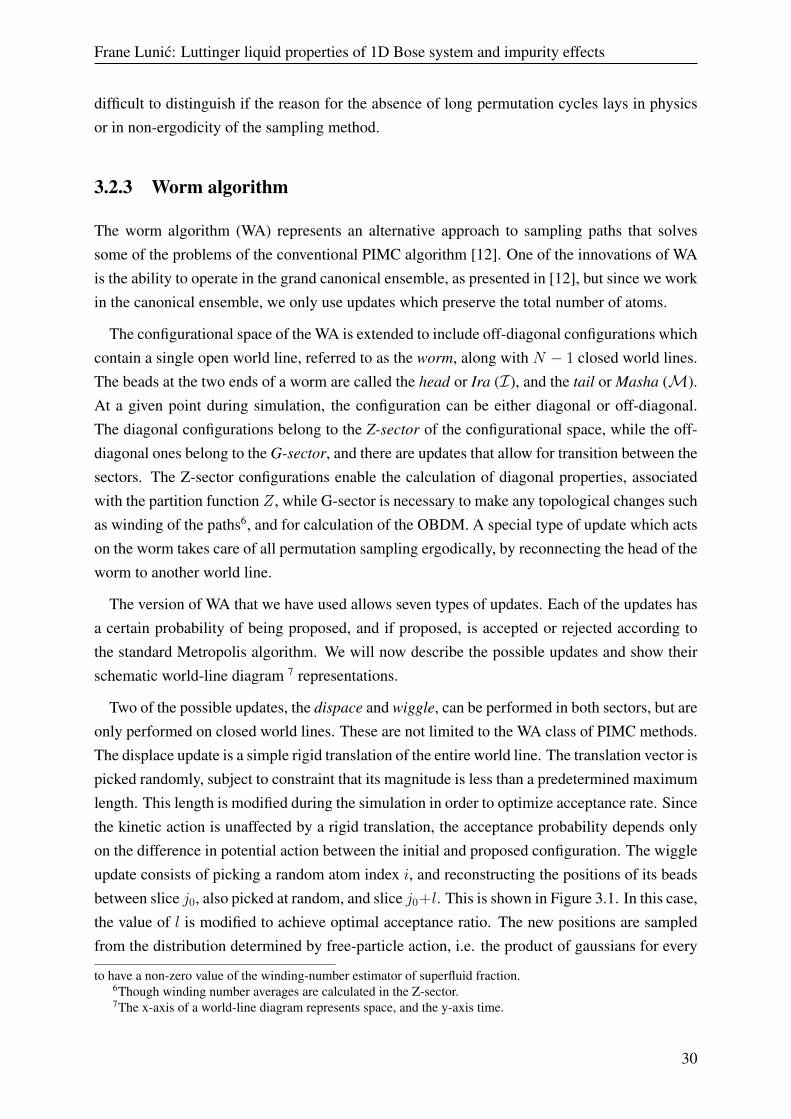
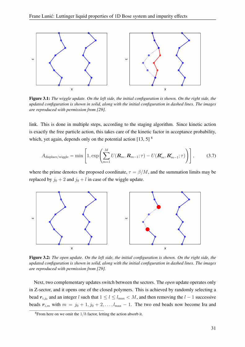
Two of the possible updates, the dispace and wiggle, can be performed in both sectors, but areonly performed on closed world lines. These are not limited to the WA class of PIMC methods.The displace update is a simple rigid translation of the entire world line. The translation vector ispicked randomly, subject to constraint that its magnitude is less than a predetermined maximumlength. This length is modified during the simulation in order to optimize acceptance rate. Sincethe kinetic action is unaffected by a rigid translation, the acceptance probability depends onlyon the difference in potential action between the initial and proposed configuration. The wiggleupdate consists of picking a random atom index i, and reconstructing the positions of its beadsbetween slice j0, also picked at random, and slice j0+l. This is shown in Figure 3.1. In this case,the value of l is modified to achieve optimal acceptance ratio. The new positions are sampledfrom the distribution determined by free-particle action, i.e. the product of gaussians for every
to have a non-zero value of the winding-number estimator of superfluid fraction.6Though winding number averages are calculated in the Z-sector.7The x-axis of a world-line diagram represents space, and the y-axis time.
30
Frane Lunic: Luttinger liquid properties of 1D Bose system and impurity effects
Figure 3.1: The wiggle update. On the left side, the initial configuration is shown. On the right side, theupdated configuration is shown in solid, along with the initial configuration in dashed lines. The imagesare reproduced with permission from [29].
link. This is done in multiple steps, according to the staging algorithm. Since kinetic actionis exactly the free particle action, this takes care of the kinetic factor in acceptance probability,which, yet again, depends only on the potential action [13, 5] 8
Adisplace/wiggle = min
[1, exp
(M∑m=1
U(Rm,Rm−1; τ)− U(R′m,R′m−1; τ)
)], (3.7)
where the prime denotes the proposed coordinate, τ = β/M , and the summation limits may bereplaced by j0 + 2 and j0 + l in case of the wiggle update.
Figure 3.2: The open update. On the left side, the initial configuration is shown. On the right side, theupdated configuration is shown in solid, along with the initial configuration in dashed lines. The imagesare reproduced with permission from [29].
Next, two complementary updates switch between the sectors. The open update operates onlyin Z-sector, and it opens one of the closed polymers. This is achieved by randomly selecting abead ri,j0 and an integer l such that 1 ≤ l ≤ lmax < M , and then removing the l − 1 successivebeads ri,m with m = j0 + 1, j0 + 2, . . . , lmax − 1. The two end beads now become Ira and
8From here on we omit the 1/~ factor, letting the action absorb it.
31

Frane Lunic: Luttinger liquid properties of 1D Bose system and impurity effects
Figure 3.3: The close update. On the left side, the initial configuration is shown, and on the right side,the updated configuration. The images are reproduced with permission from [29].
Masha. This is shown in Figure 3.2 The probability of accepting this update is
Aopen = min
[1, C
e∆U
ρ0(ri,j0+l, ri,j0 ; τ l)
], (3.8)
where ∆U is again the difference in the potential action between the initial and proposed con-figurations, and C is the constant that controls the relative statistics of the two sectors. C andlmax are simulation parameters that only affect the efficiency of the simulation [12]. On theother hand, the close update, shown in Figure 3.3, operates only in G-sector, and it reconnectsIra and Masha by constructing a path consisting of l beads between them. The number l isthe "distance" between the position of Ira and Masha in time. The path is sampled from thefree-particle distribution, and the acceptance probability is
Aclose = min
[1,ρ0(rM, rI ; τ l) e
∆U
C
]. (3.9)
The parameters lmax and C are the same as before. In this case the move has to be rejected ifl > lmax.
Figure 3.4: The advance update. On the left side, the initial configuration is shown, and on the rightside, the updated configuration. The images are reproduced with permission from [29].
32
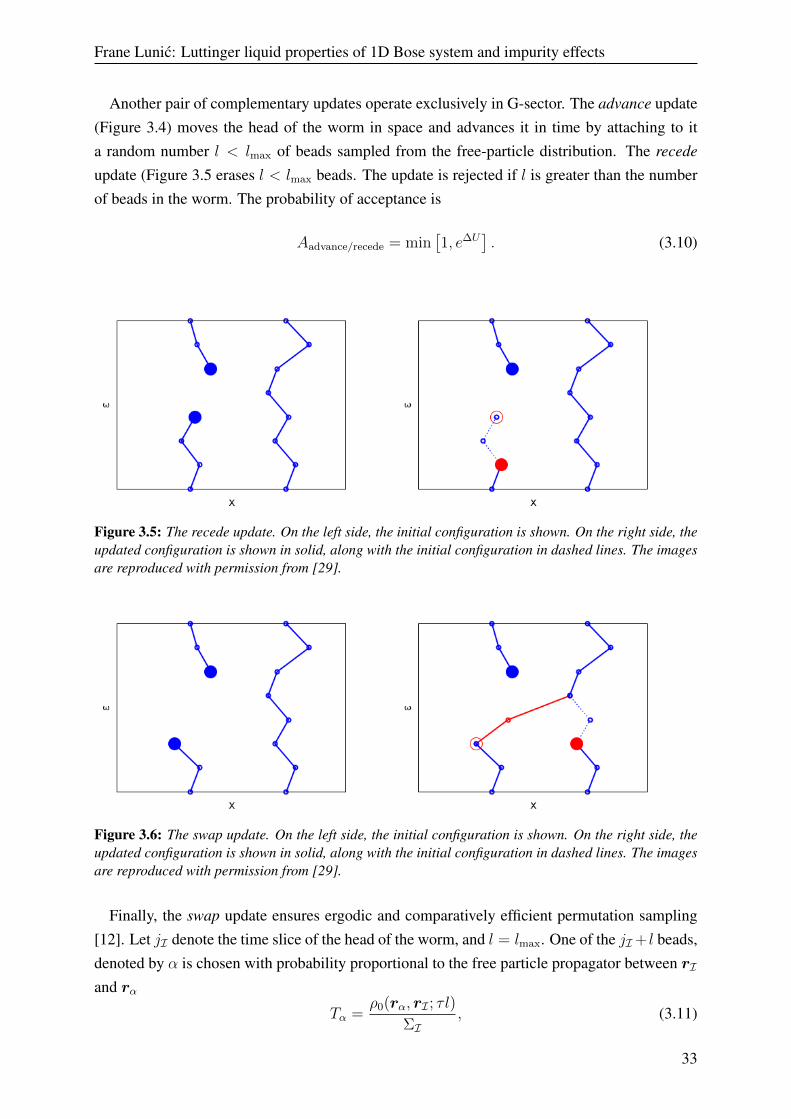
Frane Lunic: Luttinger liquid properties of 1D Bose system and impurity effects
Another pair of complementary updates operate exclusively in G-sector. The advance update(Figure 3.4) moves the head of the worm in space and advances it in time by attaching to ita random number l < lmax of beads sampled from the free-particle distribution. The recede
update (Figure 3.5 erases l < lmax beads. The update is rejected if l is greater than the numberof beads in the worm. The probability of acceptance is
Aadvance/recede = min[1, e∆U
]. (3.10)
Figure 3.5: The recede update. On the left side, the initial configuration is shown. On the right side, theupdated configuration is shown in solid, along with the initial configuration in dashed lines. The imagesare reproduced with permission from [29].
Figure 3.6: The swap update. On the left side, the initial configuration is shown. On the right side, theupdated configuration is shown in solid, along with the initial configuration in dashed lines. The imagesare reproduced with permission from [29].
Finally, the swap update ensures ergodic and comparatively efficient permutation sampling[12]. Let jI denote the time slice of the head of the worm, and l = lmax. One of the jI+ l beads,denoted by α is chosen with probability proportional to the free particle propagator between rIand rα
Tα =ρ0(rα, rI ; τ l)
ΣI, (3.11)
33
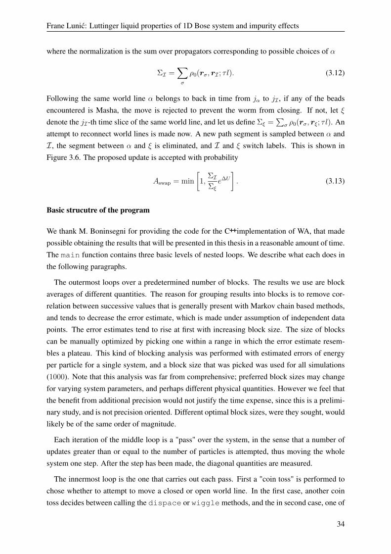
Frane Lunic: Luttinger liquid properties of 1D Bose system and impurity effects
where the normalization is the sum over propagators corresponding to possible choices of α
ΣI =∑σ
ρ0(rσ, rI ; τ l). (3.12)
Following the same world line α belongs to back in time from jα to jI , if any of the beadsencountered is Masha, the move is rejected to prevent the worm from closing. If not, let ξdenote the jI -th time slice of the same world line, and let us define Σξ =
∑σ ρ0(rσ, rξ; τ l). An
attempt to reconnect world lines is made now. A new path segment is sampled between α andI , the segment between α and ξ is eliminated, and I and ξ switch labels. This is shown inFigure 3.6. The proposed update is accepted with probability
Aswap = min
[1,
ΣIΣξ
e∆U
]. (3.13)
Basic strucutre of the program
We thank M. Boninsegni for providing the code for the C++implementation of WA, that madepossible obtaining the results that will be presented in this thesis in a reasonable amount of time.The main function contains three basic levels of nested loops. We describe what each does inthe following paragraphs.
The outermost loops over a predetermined number of blocks. The results we use are blockaverages of different quantities. The reason for grouping results into blocks is to remove cor-relation between successive values that is generally present with Markov chain based methods,and tends to decrease the error estimate, which is made under assumption of independent datapoints. The error estimates tend to rise at first with increasing block size. The size of blockscan be manually optimized by picking one within a range in which the error estimate resem-bles a plateau. This kind of blocking analysis was performed with estimated errors of energyper particle for a single system, and a block size that was picked was used for all simulations(1000). Note that this analysis was far from comprehensive; preferred block sizes may changefor varying system parameters, and perhaps different physical quantities. However we feel thatthe benefit from additional precision would not justify the time expense, since this is a prelimi-nary study, and is not precision oriented. Different optimal block sizes, were they sought, wouldlikely be of the same order of magnitude.
Each iteration of the middle loop is a "pass" over the system, in the sense that a number ofupdates greater than or equal to the number of particles is attempted, thus moving the wholesystem one step. After the step has been made, the diagonal quantities are measured.
The innermost loop is the one that carries out each pass. First a "coin toss" is performed tochose whether to attempt to move a closed or open world line. In the first case, another cointoss decides between calling the dispace or wiggle methods, and the in second case, one of
34
Frane Lunic: Luttinger liquid properties of 1D Bose system and impurity effects
the three equally likely possibilities is chosen. The first possibility calls imove which attemptseither advance or recede update, the second calls swap, and the third close. Opening a worldline will be attempted along with a worm update if the system is in Z-sector. The OBDM ismeasured in each iteration of the innermost loop. This loop is finished when two conditions aremet; the number of iterations must not be less than the number of particles and the worm mustbe closed in order to measure diagonal properties.
3.2.4 Action approximation
We have already encountered the primitive approximation for the action in section 2.2.2
e−τ(T +V) = e−τ T e−τ V , (3.14)
and we have noted that it becomes exact in the τ → 0 limit. Unfortunately, the time step τcan never be made zero in simulations, and the question of its accuracy and efficiency has tobe brought up. While simulations with small enough τ will achieve adequate convergence andsuccessful simulation can indeed be achieved with primitive action in some cases, more accurateapproximations have been developed. These approximations are appropriate for simulations oflarge systems, when it is necessary to use larger time steps to increase computational efficiency.We will only briefly present the action that is used in the particular implementation of PIMCthat we have used, as laid out in [13]. For details on action approximation methods, see [3].
The potential action of the (m+ 1)-th link takes the form
Um+1 ≡ U(Rm+1,Rm; τ) = τ
[2
3V (Rm) + V (Rm)
], (3.15)
where V (Rm) ≡∑
i<j V (|ri,m − rj,m|) is the potential energy of the system in configurationRm, assuming it can be expressed as a pairwise sum of terms, and
V (Rm) =
23V (Rm) + 2λτ2
9
∑Ni=1 (∇iV (Rm))2 , m = 2k + 1
0 , m = 2k; k = 0, 1, 2 . . . ; (3.16)
∇iV (Rm) being the gradient of the total potential energy of configuration Rm with respect tothe coordinates of the i-th particle ri,m. This action approximation is accurate up to terms oforder τ 4.
35
Chapter 4
Results
In this chapter we present a selection of the results obtained from the worm algorithm PIMCand DMC simulations as described in the previous chapter. A section is devoted to determiningthe value of the Luttinger parameter K of 1D systems of 4He (see section 3.1) atoms at threedifferent densities, and the following section presents the temperature and length dependenceof the fraction of superfluid with and without disorder.
4.1 The Luttinger parameter
In this section we analyse the data on the OBDM and the pair correlation function obtained fromPIMC, along with the DMC data on the pair correlation function, the static structure factor1, andthe dependence of the Luttinger parameter on the average density ρ0. The last is obtained fromthe compressibility, which is calculated from the equation of state at 0 K [19]. The main goal isto determine the best fit value of the Luttinger parameter.
4.1.1 The pair correlation function
The pair correlation function is defined as
g(r) = (ρ0)−2 〈ρ(r)ρ(0)〉 = (ρ0N)−1N∑i,j 6=i
〈δ(r − |ri − rj|〉 . (4.1)
1The static structure factor is the Fourier transform of the pair density correlation function, but is calculatedindependently.
36
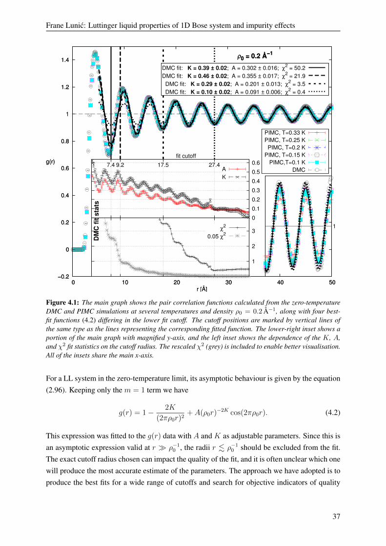
Frane Lunic: Luttinger liquid properties of 1D Bose system and impurity effects
−0.2
0
0.2
0.4
0.6
0.8
1
1.2
1.4
0 10 20 30 40 50
g(r)
r [Å]
PIMC, T=0.33 KPIMC, T=0.25 K
PIMC, T=0.2 KPIMC, T=0.15 K
PIMC,T=0.1 KDMC
ρ0 = 0.2 Å−1
−0.2
0
0.2
0.4
0.6
0.8
1
1.2
1.4
0 10 20 30 40 50
g(r)
r [Å]
DMC fit: K = 0.39 ± 0.02; A = 0.302 ± 0.016; χ2 = 50.2DMC fit: K = 0.46 ± 0.02; A = 0.355 ± 0.017; χ2 = 21.9
DMC fit: K = 0.29 ± 0.02; A = 0.201 ± 0.013; χ2 = 3.5DMC fit: K = 0.10 ± 0.02; A = 0.091 ± 0.006; χ2 = 0.4
ρ0 = 0.2 Å−1
1
2
3χ2
0.05 χ2
0
0.1
0.2
0.3
0.4
0.5
0.67.4 9.2 17.5 27.4
fit cutoff
AK
DM
C f
it s
tats
1
Figure 4.1: The main graph shows the pair correlation functions calculated from the zero-temperatureDMC and PIMC simulations at several temperatures and density ρ0 = 0.2Å−1, along with four best-fit functions (4.2) differing in the lower fit cutoff. The cutoff positions are marked by vertical lines ofthe same type as the lines representing the corresponding fitted function. The lower-right inset shows aportion of the main graph with magnified y-axis, and the left inset shows the dependence of the K, A,and χ2 fit statistics on the cutoff radius. The rescaled χ2 (grey) is included to enable better visualisation.All of the insets share the main x-axis.
For a LL system in the zero-temperature limit, its asymptotic behaviour is given by the equation(2.96). Keeping only the m = 1 term we have
g(r) = 1− 2K
(2πρ0r)2+ A(ρ0r)
−2K cos(2πρ0r). (4.2)
This expression was fitted to the g(r) data with A and K as adjustable parameters. Since this isan asymptotic expression valid at r � ρ−1
0 , the radii r . ρ−10 should be excluded from the fit.
The exact cutoff radius chosen can impact the quality of the fit, and it is often unclear which onewill produce the most accurate estimate of the parameters. The approach we have adopted is toproduce the best fits for a wide range of cutoffs and search for objective indicators of quality
37

Frane Lunic: Luttinger liquid properties of 1D Bose system and impurity effects
0 20 40 60 80
100 120 140
0 10 20 30 40 50
χ2
r [Å]
χ2
0.05 χ2
ρ0 = 0.2
0
0.1
0.2
0.3
0.4
0.5
0.6
0.7
K
PIMC, T = 0.2 KPIMC, T = 0.33 K
PIMC, T = 0.1 KDMC, T = 0 K
ρ0 = 0.2
Figure 4.2: The figure shows the dependence of the PIMC χ2 andK fit statistics at density ρ0 = 0.2Å−1
and temperature T = 0.1K on lower fit cutoff. The χ2 is shown in the lower graph alongside with itsrescaled values (grey) to enable better visualisation. Additionally, in the upper graph, the K values ofseveral higher temperatures (color) are shown to demonstrate the convergence, and the DMC K valuesare shown for comparison (grey).
of the fit, i.e. the reduced2 chi-square values (χ2) and the stability of the best-fit parameters, aswell as the visual correspondence to the plotted data. When there is a lot of variance betweenthe results, and no obvious way to determine the most correct result, we attempt to asses thereasonable interval for the value of K.
We start with the system at density ρ0 = 0.2 Å−1. The PIMC and DMC data are givenin Figure 4.1, along with curves fitted to the DMC data for various fit cutoffs. The decayingoscillation of the g(r) characteristic of liquid systems can be seen from the main plot, butthe decay appeares to cease at large radii for the DMC data. The PIMC data shows a slightdependence of the amplitude of the peaks on temperature, as can be seen magnified in thebottom-right inset, and the agreement between the zero-temperature DMC and the PIMC dataat the lowest temperatures is very good. However, though the decay of oscillation is slow,it does not appear to completely cease for PIMC. This could perhaps be a finite temperatureeffect, but it is likely that the cessation of the decay is a method-specific numeric effect sincethe low K values it requires are inconsistent with the rest of the results. The left inset shows thedependence of the DMC fit statistics, namely the χ2 and the fit parameters, on the cutoff radius.The K parameter drops from around 0.6 to 0, and there appears to be no range of stable valuesof the fit parameters. The χ2 values are large for lower cutoffs, and become of order ∼ 1 close
2Divided by the number of degrees of freedom.
38

Frane Lunic: Luttinger liquid properties of 1D Bose system and impurity effects
to radius L/2. However this region corresponds to unlikely low values of K, close to zero. It isworth noting that the large χ2 values may be due to underestimate of the uncertainty in the data,but we did not attempt to verify this possibility. The PIMC fit statistics are shown in Figure 4.2.In this case, the values of fit parameters are somewhat more stable, and the global minimum ofχ2 corresponds to K ∼ 0.4. The PIMC and DMC fits produce similar results up to about L/8radius (K ∼ 0.3-0.6). We will see from comparison with the structure factor and equation ofstate results that it is indeed likely that the actual parameter is within a similar range. We alsonote that the majority of attempted fits, and all of the DMC fits with χ2 less than two orders ofmagnitude greater than the minimum (excluding regions of high instability on the right side ofFigure 4.2) give the value of K less than 0.5.
0
0.2
0.4
0.6
0.8
1
1.2
0 10 20 30 40 50 60 70 80
g(r)
r [Å]
PIMC, T = 0.2 KPIMC, T = 0.1 K
PIMC, T = 0.08 KDMC
ρ0 = 0.125 Å−1
0
0.2
0.4
0.6
0.8
1
1.2
0 10 20 30 40 50 60 70 80
g(r)
r [Å]
DMC fit: K = 1.40 ± 0.03; A = 0.015 ± 0.003; χ2 = 2.3DMC fit: K = 1.65 ± 0.03; A = −0.010 ± 0.009; χ2 = 0.8
ρ0 = 0.125 Å−1
0.5
1χ
2
0.20 χ2
0
0.5
1
1.5
2
2.510.4 17.0
fit cutoff
AK
DM
C f
it s
tats
1 0.951 0.95
Figure 4.3: The main graph shows the pair correlation functions calculated from the zero-temperatureDMC and PIMC simulations at several temperatures and density ρ0 = 0.125Å−1, along with two best-fit functions (4.2) differing in the lower fit cutoff. The cutoff positions are marked by vertical lines ofthe same type as the lines representing the corresponding fitted function. The lower-right inset shows aportion of the main graph with magnified y-axis (rotated by 90◦ anticlockwise), and the left inset showsthe dependence of the K, A, and χ2 fit statistics on the cutoff radius. The rescaled χ2 (grey) is includedto enable better visualisation. The left inset shares the main x-axis.
In Figure 4.3 we show the DMC and PIMC data on pair correlation functions at density
39
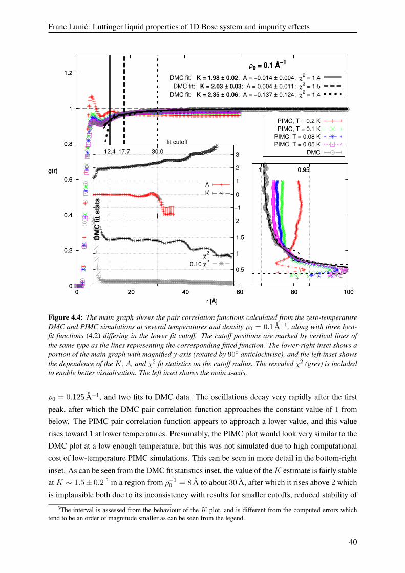
Frane Lunic: Luttinger liquid properties of 1D Bose system and impurity effects
0
0.2
0.4
0.6
0.8
1
1.2
0 20 40 60 80 100
g(r)
r [Å]
PIMC, T = 0.2 KPIMC, T = 0.1 K
PIMC, T = 0.08 KPIMC, T = 0.05 K
DMC
ρ0 = 0.1 Å−1
0
0.2
0.4
0.6
0.8
1
1.2
0 20 40 60 80 100
g(r)
r [Å]
DMC fit: K = 1.98 ± 0.02; A = −0.014 ± 0.004; χ2 = 1.4DMC fit: K = 2.03 ± 0.03; A = 0.004 ± 0.011; χ2 = 1.5
DMC fit: K = 2.35 ± 0.06; A = −0.137 ± 0.124; χ2 = 1.4
ρ0 = 0.1 Å−1
0.5
1
1.5
2
χ2
0.10 χ2
−1
0
1
2
312.4 17.7 30.0
fit cutoff
AK
DM
C f
it s
tats
1 0.951 0.95
Figure 4.4: The main graph shows the pair correlation functions calculated from the zero-temperatureDMC and PIMC simulations at several temperatures and density ρ0 = 0.1Å−1, along with three best-fit functions (4.2) differing in the lower fit cutoff. The cutoff positions are marked by vertical lines ofthe same type as the lines representing the corresponding fitted function. The lower-right inset shows aportion of the main graph with magnified y-axis (rotated by 90◦ anticlockwise), and the left inset showsthe dependence of the K, A, and χ2 fit statistics on the cutoff radius. The rescaled χ2 (grey) is includedto enable better visualisation. The left inset shares the main x-axis.
ρ0 = 0.125 Å−1, and two fits to DMC data. The oscillations decay very rapidly after the firstpeak, after which the DMC pair correlation function approaches the constant value of 1 frombelow. The PIMC pair correlation function appears to approach a lower value, and this valuerises toward 1 at lower temperatures. Presumably, the PIMC plot would look very similar to theDMC plot at a low enough temperature, but this was not simulated due to high computationalcost of low-temperature PIMC simulations. This can be seen in more detail in the bottom-rightinset. As can be seen from the DMC fit statistics inset, the value of theK estimate is fairly stableat K ∼ 1.5± 0.2 3 in a region from ρ−1
0 = 8 Å to about 30 Å, after which it rises above 2 whichis implausible both due to its inconsistency with results for smaller cutoffs, reduced stability of
3The interval is assessed from the behaviour of the K plot, and is different from the computed errors whichtend to be an order of magnitude smaller as can be seen from the legend.
40

Frane Lunic: Luttinger liquid properties of 1D Bose system and impurity effects
both parameter estimates, and disagreement with estimates obtained from other methods. Theχ2 values are close to one at around 15 Å and up to 20 Å, indicating good fit quality. We omitthe discussion of fits to the PIMC data since they are necessarily of lesser quality due to thediscussed finite-temperature effects.
Nearly everything stated in the previous paragraph applies as well to the ρ0 = 0.1 Å−1 case,and the graphs are shown in Figure 4.4. In this case, the K estimate can be given at aroundor slightly above 2, but less than 2.5. The χ2 values are approximately 1.5, which is less thanideal for a large number of degrees of freedom 4, but probably low enough to allow a decent fitquality.
4.1.2 The structure factor
0
0.2
0.4
0.6
0.8
1
1.2
0 0.2 0.4 0.6 0.8 1 1.2 1.4
S(q)
q [Å−1]
ρ0 = 0.2 Å−1
DMC
K = 0.513 ± 0.005; χ2 = 0.6K = 0.491 ± 0.008; χ2 = 5.1K = 0.482 ± 0.006; χ2 = 5.4K = 0.477 ± 0.004; χ2 = 4.7K = 0.479 ± 0.004; χ2 = 5.0
1
2
3
4
5
0.17 0.3 0.42 0.6 0.67
χ2
0.49
0.51
fit cutoff
K
0.2 0.4 0.6 0.8
1 1.2 1.4 1.6 1.8
2 1 2 3 4 5 6 7 8 9
S(q)
Figure 4.5: The main graph shows the results of the DMC calculation of the static structure factor at lowq and density ρ0 = 0.2Å−1, along with several lines representing the best fit of (4.4) to the low q dataup to various values of upper fit cutoffs qc. The qc positions are marked by vertical lines of the same typeas the lines representing the corresponding fitted function. The bottom-right inset shows the full range ofq, and the insets on the top left graphically show the dependence of fit statistics on the selected qc. Theleftmost K estimate comes from the linear interpolation between q = 0, and the first q point.
4The table of critical values of nonreduced χ2 can be found at http://www.itl.nist.gov/div898/handbook/eda/section3/eda3674.htm
41
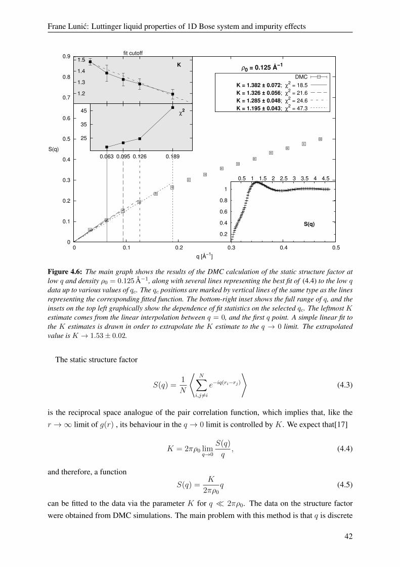
Frane Lunic: Luttinger liquid properties of 1D Bose system and impurity effects
0
0.1
0.2
0.3
0.4
0.5
0.6
0.7
0.8
0.9
0 0.1 0.2 0.3 0.4 0.5
S(q)
q [Å−1]
ρ0 = 0.125 Å−1
DMC
K = 1.382 ± 0.072; χ2 = 18.5K = 1.326 ± 0.056; χ2 = 21.6K = 1.285 ± 0.048; χ2 = 24.6K = 1.195 ± 0.043; χ2 = 47.3
25
35
45
0.063 0.095 0.126 0.189
χ2
1.2
1.3
1.4
1.5fit cutoff
K
0.2
0.4
0.6
0.8
1
0.5 1 1.5 2 2.5 3 3.5 4 4.5
S(q)
Figure 4.6: The main graph shows the results of the DMC calculation of the static structure factor atlow q and density ρ0 = 0.125Å−1, along with several lines representing the best fit of (4.4) to the low qdata up to various values of qc. The qc positions are marked by vertical lines of the same type as the linesrepresenting the corresponding fitted function. The bottom-right inset shows the full range of q, and theinsets on the top left graphically show the dependence of fit statistics on the selected qc. The leftmost Kestimate comes from the linear interpolation between q = 0, and the first q point. A simple linear fit tothe K estimates is drawn in order to extrapolate the K estimate to the q → 0 limit. The extrapolatedvalue is K → 1.53± 0.02.
The static structure factor
S(q) =1
N
⟨N∑i,j 6=i
e−iq(ri−rj)
⟩(4.3)
is the reciprocal space analogue of the pair correlation function, which implies that, like ther →∞ limit of g(r) , its behaviour in the q → 0 limit is controlled by K. We expect that[17]
K = 2πρ0 limq→0
S(q)
q, (4.4)
and therefore, a function
S(q) =K
2πρ0
q (4.5)
can be fitted to the data via the parameter K for q � 2πρ0. The data on the structure factorwere obtained from DMC simulations. The main problem with this method is that q is discrete
42
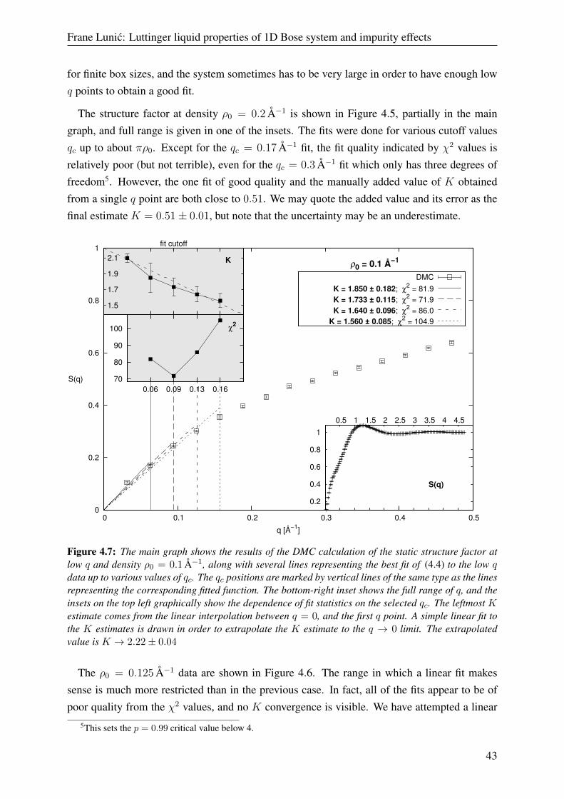
Frane Lunic: Luttinger liquid properties of 1D Bose system and impurity effects
for finite box sizes, and the system sometimes has to be very large in order to have enough lowq points to obtain a good fit.
The structure factor at density ρ0 = 0.2 Å−1 is shown in Figure 4.5, partially in the maingraph, and full range is given in one of the insets. The fits were done for various cutoff valuesqc up to about πρ0. Except for the qc = 0.17 Å−1 fit, the fit quality indicated by χ2 values isrelatively poor (but not terrible), even for the qc = 0.3 Å−1 fit which only has three degrees offreedom5. However, the one fit of good quality and the manually added value of K obtainedfrom a single q point are both close to 0.51. We may quote the added value and its error as thefinal estimate K = 0.51± 0.01, but note that the uncertainty may be an underestimate.
0
0.2
0.4
0.6
0.8
1
0 0.1 0.2 0.3 0.4 0.5
S(q)
q [Å−1]
ρ0 = 0.1 Å−1
DMC
K = 1.850 ± 0.182; χ2 = 81.9K = 1.733 ± 0.115; χ2 = 71.9K = 1.640 ± 0.096; χ2 = 86.0
K = 1.560 ± 0.085; χ2 = 104.9
70
80
90
100
0.06 0.09 0.13 0.16
χ2
1.5
1.7
1.9
2.1
fit cutoff
K
0.2
0.4
0.6
0.8
1
0.5 1 1.5 2 2.5 3 3.5 4 4.5
S(q)
Figure 4.7: The main graph shows the results of the DMC calculation of the static structure factor atlow q and density ρ0 = 0.1Å−1, along with several lines representing the best fit of (4.4) to the low qdata up to various values of qc. The qc positions are marked by vertical lines of the same type as the linesrepresenting the corresponding fitted function. The bottom-right inset shows the full range of q, and theinsets on the top left graphically show the dependence of fit statistics on the selected qc. The leftmost Kestimate comes from the linear interpolation between q = 0, and the first q point. A simple linear fit tothe K estimates is drawn in order to extrapolate the K estimate to the q → 0 limit. The extrapolatedvalue is K → 2.22± 0.04
The ρ0 = 0.125 Å−1 data are shown in Figure 4.6. The range in which a linear fit makessense is much more restricted than in the previous case. In fact, all of the fits appear to be ofpoor quality from the χ2 values, and no K convergence is visible. We have attempted a linear
5This sets the p = 0.99 critical value below 4.
43
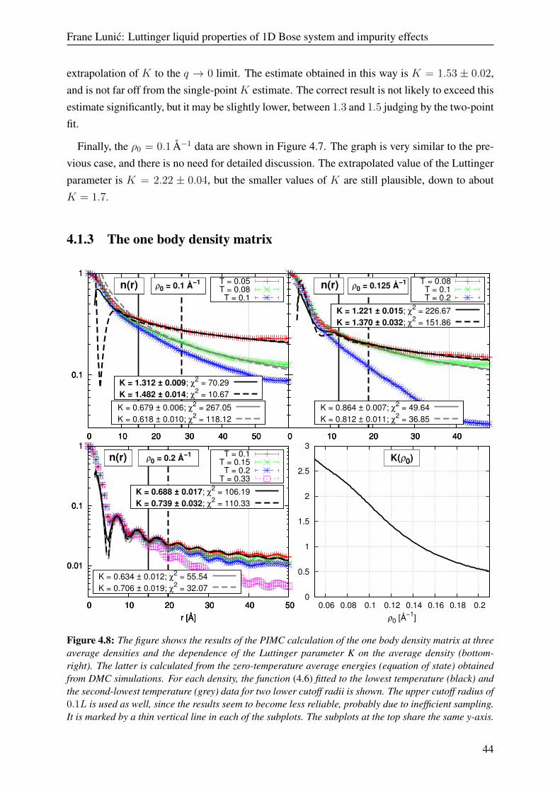
Frane Lunic: Luttinger liquid properties of 1D Bose system and impurity effects
extrapolation of K to the q → 0 limit. The estimate obtained in this way is K = 1.53 ± 0.02,and is not far off from the single-point K estimate. The correct result is not likely to exceed thisestimate significantly, but it may be slightly lower, between 1.3 and 1.5 judging by the two-pointfit.
Finally, the ρ0 = 0.1 Å−1 data are shown in Figure 4.7. The graph is very similar to the pre-vious case, and there is no need for detailed discussion. The extrapolated value of the Luttingerparameter is K = 2.22 ± 0.04, but the smaller values of K are still plausible, down to aboutK = 1.7.
4.1.3 The one body density matrix
0.1
1
0 10 20 30 40 50
T = 0.05T = 0.08T = 0.1
n(r) ρ0 = 0.1 Å−1
0.1
1
0 10 20 30 40 50
K = 0.679 ± 0.006; χ2 = 267.05K = 0.618 ± 0.010; χ2 = 118.12
n(r) ρ0 = 0.1 Å−1
0.1
1
0 10 20 30 40 50
K = 1.312 ± 0.009; χ2 = 70.29K = 1.482 ± 0.014; χ2 = 10.67
n(r) ρ0 = 0.1 Å−1
0 10 20 30 40
T = 0.08T = 0.1T = 0.2
n(r) ρ0 = 0.125 Å−1
0 10 20 30 40
K = 0.864 ± 0.007; χ2 = 49.64K = 0.812 ± 0.011; χ2 = 36.85
n(r) ρ0 = 0.125 Å−1
0 10 20 30 40
K = 1.221 ± 0.015; χ2 = 226.67K = 1.370 ± 0.032; χ2 = 151.86
n(r) ρ0 = 0.125 Å−1
0.01
0.1
1
0 10 20 30 40 50
r [Å]
T = 0.1T = 0.15T = 0.2
T = 0.33
n(r) ρ0 = 0.2 Å−1
0.01
0.1
1
0 10 20 30 40 50
r [Å]
K = 0.634 ± 0.012; χ2 = 55.54K = 0.706 ± 0.019; χ2 = 32.07
n(r) ρ0 = 0.2 Å−1
0.01
0.1
1
0 10 20 30 40 50
r [Å]
K = 0.688 ± 0.017; χ2 = 106.19K = 0.739 ± 0.032; χ2 = 110.33
n(r) ρ0 = 0.2 Å−1
0
0.5
1
1.5
2
2.5
3
0.06 0.08 0.1 0.12 0.14 0.16 0.18 0.2
ρ0 [Å−1]
K(ρ0)
Figure 4.8: The figure shows the results of the PIMC calculation of the one body density matrix at threeaverage densities and the dependence of the Luttinger parameter K on the average density (bottom-right). The latter is calculated from the zero-temperature average energies (equation of state) obtainedfrom DMC simulations. For each density, the function (4.6) fitted to the lowest temperature (black) andthe second-lowest temperature (grey) data for two lower cutoff radii is shown. The upper cutoff radius of0.1L is used as well, since the results seem to become less reliable, probably due to inefficient sampling.It is marked by a thin vertical line in each of the subplots. The subplots at the top share the same y-axis.
44
Frane Lunic: Luttinger liquid properties of 1D Bose system and impurity effects
The one body density matrix was defined in (2.7), and here we present the PIMC results onthe OBDM normalized by particle density n(|r′ − r′′|), so that its value at n(r = 0) is 1. Thelong-range behaviour in the Luttinger model is given by (2.97), or keeping only first two terms
n(r) = (ρ0x)−1
2K
[B0 +B1(ρ0r)
−2K cos(2πρ0r)]. (4.6)
Fitting (4.6) to the data mostly produced fits of poor quality. We show the fits for the lowestand the second lowest available temperature in Figure 4.8. There is no evidence of convergencetoward zero-temperature values of K, except in the case of ρ0 = 0.2 Å−1 shown in the bottom-left corner. This is not surprising as we have already seen from the g(r) results that the simulatedtemperatures are not low enough. The value obtained in the ρ0 = 0.2 Å−1 case is between0.65 and 0.75 which is slightly above previous estimates, and in the case of ρ0 = 0.125 Å−1,the estimated interval is between 1.2 and 1.4, slightly below previous estimates. While theseresults are not too far off from the previous estimates, the result for the density ρ0 = 0.1 Å−1 issignificantly lower than before at K . 1.5. Clearly, significantly lower temperature is requiredto successfully approximate the pair correlation function and the OBDM at such a low density.However, since the K estimates tend to rise as the temperature decreases, this can be taken asevidence that K > 1 at ρ0 = 0.1 Å−1 and ρ0 = 0.125 Å−1.
4.1.4 Summary
Here we summarise the results on the Luttinger parameter, and state what may be concludedabout its value.
ρ0 = 0.2 Å−1 The fits to the pair correlation function seem to imply the value in the (0.3, 0.6)
interval, based on combination of PIMC and DMC data, with the PIMC data showingmore stability, and is awarded more weight. The DMC static structure factor data leads toa consistent result K = 0.51±0.01, as well as the DMC equation of state which suggestsa value between 0.5 and 0.6, as can be read from Figure 4.8. Only the PIMC OBDM datasuggest a value above 0.6, and the fits are of low quality. We conclude that the value ofK is likely to be in the interval (0.4, 0.6), and it is almost certainly less than 1, which willbe relevant after introducing disorder.
ρ0 = 0.125 Å−1 Here the DMC g(r) data suggests that K is likely to be in the (1.3, 1.7)
interval, the structure factor data suggests a similar interval (1.3, 1.6), and the equationof state gives a value between 1.2 and 1.3. The OBDM gives an interval of (1.2, 1.4),but with low fit quality and questionable convergence to zero-temperature behaviour. Kis almost certainly above 1, but it is impossible to verify with available data whether it isbelow 1.5. Its value probably lies in the interval (1.2, 1.6).
45
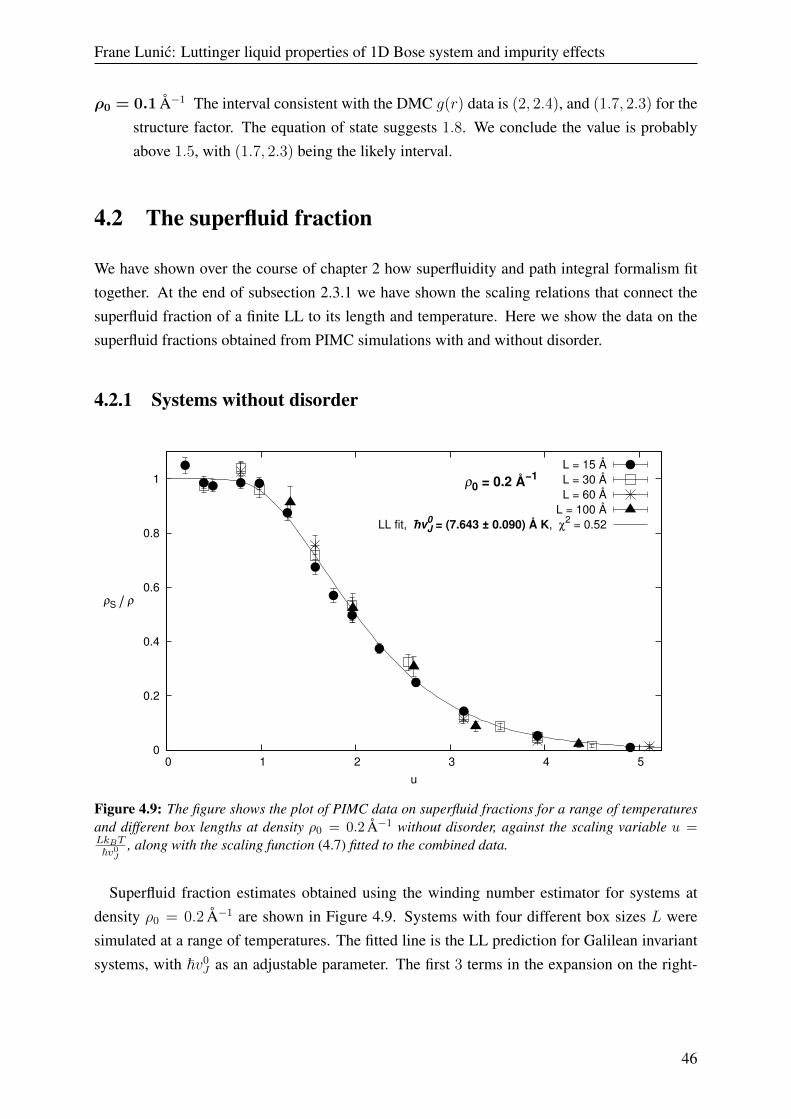
Frane Lunic: Luttinger liquid properties of 1D Bose system and impurity effects
ρ0 = 0.1 Å−1 The interval consistent with the DMC g(r) data is (2, 2.4), and (1.7, 2.3) for thestructure factor. The equation of state suggests 1.8. We conclude the value is probablyabove 1.5, with (1.7, 2.3) being the likely interval.
4.2 The superfluid fraction
We have shown over the course of chapter 2 how superfluidity and path integral formalism fittogether. At the end of subsection 2.3.1 we have shown the scaling relations that connect thesuperfluid fraction of a finite LL to its length and temperature. Here we show the data on thesuperfluid fractions obtained from PIMC simulations with and without disorder.
4.2.1 Systems without disorder
0
0.2
0.4
0.6
0.8
1
0 1 2 3 4 5
ρS / ρ
u
ρ0 = 0.2 Å−1L = 15 ÅL = 30 ÅL = 60 Å
L = 100 ÅLL fit, −hvJ
0 = (7.643 ± 0.090) Å K, χ2 = 0.52
Figure 4.9: The figure shows the plot of PIMC data on superfluid fractions for a range of temperaturesand different box lengths at density ρ0 = 0.2Å−1 without disorder, against the scaling variable u =LkBT~v0J
, along with the scaling function (4.7) fitted to the combined data.
Superfluid fraction estimates obtained using the winding number estimator for systems atdensity ρ0 = 0.2 Å−1 are shown in Figure 4.9. Systems with four different box sizes L weresimulated at a range of temperatures. The fitted line is the LL prediction for Galilean invariantsystems, with ~v0
J as an adjustable parameter. The first 3 terms in the expansion on the right-
46

Frane Lunic: Luttinger liquid properties of 1D Bose system and impurity effects
hand side of (2.101) were kept, resulting in the expression
ρSρ
= 1− 8π
u
e−2πu + 4e−8πu
1 + 2e−2πu + 2e−8πu, (4.7)
where u = LkBT~v0J
. The fit is quite good, which means that there is no significant depen-dence on either L or T separate from the scaling variable u. The expected value of ~vJ ,~v0
J = 2πλρ0 = 7, 61477, is within one standard error of the estimated value of the fit parame-ter, ~v0
J = (7.64± 0.09) Å K.
0
0.2
0.4
0.6
0.8
1
ρS / ρρ0 = 0.2 Å−1
Gaussian: ε = 10 K, σ = 0.25 Å, L = 30 ÅFit (ε = 10 K, L = 30 Å), vJ/vJ0 = 0.839 ± 0.039, χ2 = 149.35
Gaussian: ε = 10 K, σ = 0.25 Å, L = 60 ÅFit (ε = 10 K, L = 60 Å), vJ/vJ0 = 0.770 ± 0.035, χ2 = 47.92
Gaussian: ε = 10 K, σ = 0.25 Å, L = 90 ÅFit (ε = 10 K, L = 90 Å), vJ/vJ0 = 0.709 ± 0.040, χ2 = 35.35
Gaussian: ε = 50 K, σ = 0.25 Å, L = 30 ÅGaussian: ε = 50 K, σ = 0.25 Å, L = 60 Å
Gaussian: ε = 2 K, σ = 0.25 Å, L = 30 ÅGaussian: ε = 2 K, σ = 0.25 Å, L = 60 Å
0
0.2
0.4
0.6
0.8
1
ρS / ρρ0 = 0.2 Å−1
Lennard Jones: ε = 0.1, σ = 1 Å, L=30 ÅLennard Jones: ε = 0.1, σ = 1 Å, L=60 Å
No disorder, −hvJ = −hvJ0 = 7.615
0
0.2
0.4
0.6
0.8
1
ρS / ρρ0 = 0.2 Å−1
0
0.05
0.1
0.15
0.5 1 1.5 2 2.5 3 3.5 4 4.5 5u0
ρ0 = 0.2 Å−1
0
0.05
0.1
0.15
0.5 1 1.5 2 2.5 3 3.5 4 4.5 5u0
ρ0 = 0.2 Å−1
Gaussian: ε = 50 K, σ = 0.25 Å, L = 30 ÅFit (ε = 50 K, L = 30 Å), vJ/vJ0 = 0.330 ± 0.042, χ2 = 260.16
Gaussian: ε = 50 K, σ = 0.25 Å, L = 60 ÅFit (ε = 50 K, L = 60 Å), vJ/vJ0 = 0.358 ± 0.033, χ2 = 52.15
0
0.05
0.1
0.15
0.5 1 1.5 2 2.5 3 3.5 4 4.5 5u0
ρ0 = 0.2 Å−1
Figure 4.10: The top panel shows the plot of PIMC data on superfluid fractions against the variableu0 = LkBT
~v0Jfor systems of various lengths and temperatures (ρ0 = 0.2Å−1) with a single disorder
particle. The potential between the disorder particle and regular atoms is either Gaussian-shaped (color)or the Lennard-Jones potential (black), with the potential parameters given in the legend. Fits of thescaling function (4.8) to the Gaussian disorder (ε = 10K) data are shown in the same color as the pointsfor each box length, and the theoretical prediction for a Galilean invariant system without disorder isshown in grey. The bottom panel shows the fits to the ε = 50K data. Both panels share the same x-axes.The data points are the average of several (n) simulations with different randomly selected positions of
the impurity. The errors are calculated from σ = 1n
√∑ni σ
2i .
47

Frane Lunic: Luttinger liquid properties of 1D Bose system and impurity effects
4.2.2 Systems with disorder
We begin by noting that the additional particle of impurity is expected to have the effect ofdecreasing effective density by excluding a part of the volume. However, if simply the rangeof the disorder potential is excluded in calculation of ρ0, the effect on the results is of littlesignificance.
0
0.1
0.2
0.3
0.4
0.5
0.6
0.7
0.8
ρS / ρ ρ0 = 0.125 Å−1
ε = 10 K, σ = 0.25 Å
L = 32 ÅFit (L = 32 Å), vJ /vJ
0 = 0.807 ± 0.017, χ2 = 58.74
L = 56 ÅFit (L = 56 Å), vJ /vJ
0 = 0.817 ± 0.010, χ2 = 9.93
L = 72 ÅNo disorder, −hvJ = −hvJ
0 = 4.759
0
0.1
0.2
0.3
0.4
0.5
0.6
0.7
0.8
ρS / ρ ρ0 = 0.125 Å−1
ε = 10 K, σ = 0.25 Å
0
0.05
0.1
0.15
0.2
0.5 1 1.5 2 2.5 3 3.5 4 4.5 5
ρS / ρ
u0
ρ0 = 0.125 Å−1
ε = 50 K, σ = 0.25 Å
L = 32 ÅFit (L = 32 Å), vJ /vJ
0 = 0.317 ± 0.028, χ2 = 240.04
L = 56 ÅFit (L = 56 Å), vJ /vJ
0 = 0.480 ± 0.026, χ2 = 40.74
L = 72 ÅNo disorder, −hvJ = −hvJ
0 = 4.759
0
0.05
0.1
0.15
0.2
0.5 1 1.5 2 2.5 3 3.5 4 4.5 5
ρS / ρ
u0
ρ0 = 0.125 Å−1
ε = 50 K, σ = 0.25 Å
Figure 4.11: The top panel shows the plot of PIMC data on superfluid fractions against the scalingvariable u0 = LkBT
~v0Jfor systems of various lengths and temperatures (ρ0 = 0.125Å−1) with a single
disorder particle. The potential between the disorder particle and regular atoms is Gaussian-shapedwith ε = 10K. Fits of the scaling function (4.8) to the data for two of the box lengths are shown, andthe theoretical prediction for a Galilean invariant system without disorder is shown in grey. The bottompanel shows the fits to the ε = 50K data. Both panels share the same x-axes. The data points are theaverage of several (n) simulations with different randomly selected positions of the impurity. The errors
are calculated from σ = 1n
√∑ni σ
2i .
The scaling relation used in previous subsections assumes Galilean invariance, and requiresthat ρS/ρ → 1 as T → 0. Instead, we fit the data on systems with disorder to the expression
48
Frane Lunic: Luttinger liquid properties of 1D Bose system and impurity effects
(2.100), keeping only the first three terms in expansion:
ρSρ
=2πLkBT
~v0J
exp(−π
2u0
v0JvJ
)+ 4 exp
(−4π
2u0
v0JvJ
)1 + 2 exp
(−π
2u0
v0JvJ
)+ 2 exp
(−4π
2u0
v0JvJ
) , (4.8)
v0J/vJ being an adjustable parameter, and u0 v
0J/vJ = u.
In Figure 4.10 we see the superfluid fraction data for ρ0 = 0.2 Å−1 systems with disorder ofvarying "magnitude"6 , represented by the normalization parameter ε of the Gaussian potential.Evidently, the magnitude of the disorder affects the resulting fraction, but the fraction does notvanish, except in the case of the unbounded LJ potential. The fractions are very weakly affectedin case of ε = 2 K, which is an order of magnitude larger than the measured average energiesper particle at this density (∼ 0.4K). The disorder of ε = 10 K magnitude visibly destroysthe u-scaling. The different box lengths are differently affected, with the fraction being moresuppressed for larger lengths. The fits to the scaling relation are visibly poor, and χ2 values arehigh. The fractions of systems with ε = 50 K are almost completely suppressed.
The top and bottom panels in Figure 4.11 show the ρ0 = 0.125 Å−1 data for different disordermagnitudes. The lower-magnitude data on the top appear to be better described by the scalingrelation than the ρ0 = 0.2 Å−1 data. However, there is visible disagreement between the fits andthe data, especially in the low u region, and the χ2 values are still quite high (although lowerfor each box length than earlier). The bottom, higher-magnitude data does not show any indi-cation of obeying the predicted scaling relation. However, in both cases there is little differencebetween different box lengths, as evidenced by the nearly same value of the fit parameter in thelower-magnitude case.
The same discussion applies to the ρ0 = 0.1 Å−1 case in Figure 4.12. The deviation from thescaling relation fit is qualitatively the same as in the previous case. However, we see slightlybetter evidence of breakdown of u-scaling, since the ρS/ρ values in the bottom panel appearslightly more suppressed for larger box length.
In summary, addition of disorder suppresses the values of the superfluid fraction and, at leastin case of ρ0 = 0.2 Å−1 for which K < 1, destroys the u-scaling. For the two lower densities(K > 1), the scaling appears to be mostly, but perhaps not entirely, preserved. The discussedscaling relation fits the lower-magnitude disorder data better, but there are visible deviations.
6We introduce this as an internal shorthand to differentiate between cases differing exclusively in the normal-ization parameter of the Gaussian.
49
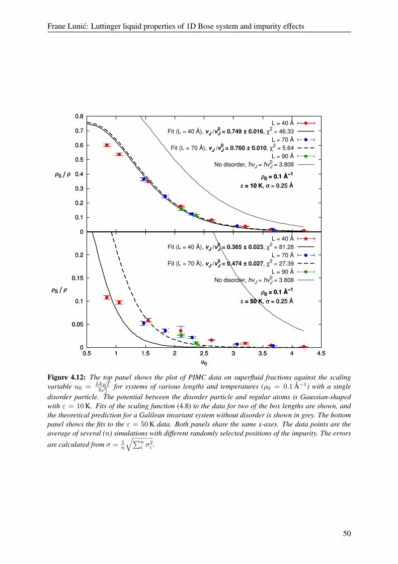
Frane Lunic: Luttinger liquid properties of 1D Bose system and impurity effects
0
0.1
0.2
0.3
0.4
0.5
0.6
0.7
0.8
ρS / ρ ρ0 = 0.1 Å−1
ε = 10 K, σ = 0.25 Å
L = 40 ÅFit (L = 40 Å), vJ /vJ
0 = 0.749 ± 0.016, χ2 = 46.33
L = 70 ÅFit (L = 70 Å), vJ /vJ
0 = 0.760 ± 0.010, χ2 = 5.64
L = 90 ÅNo disorder, −hvJ = −hvJ
0 = 3.808
0
0.1
0.2
0.3
0.4
0.5
0.6
0.7
0.8
ρS / ρ ρ0 = 0.1 Å−1
ε = 10 K, σ = 0.25 Å
0
0.05
0.1
0.15
0.2
0.5 1 1.5 2 2.5 3 3.5 4 4.5
ρS / ρ
u0
ρ0 = 0.1 Å−1
ε = 50 K, σ = 0.25 Å
L = 40 ÅFit (L = 40 Å), vJ /vJ
0 = 0.365 ± 0.023, χ2 = 81.28
L = 70 ÅFit (L = 70 Å), vJ /vJ
0 = 0.474 ± 0.027, χ2 = 27.39
L = 90 ÅNo disorder, −hvJ = −hvJ
0 = 3.808
0
0.05
0.1
0.15
0.2
0.5 1 1.5 2 2.5 3 3.5 4 4.5
ρS / ρ
u0
ρ0 = 0.1 Å−1
ε = 50 K, σ = 0.25 Å
Figure 4.12: The top panel shows the plot of PIMC data on superfluid fractions against the scalingvariable u0 = LkBT
~v0Jfor systems of various lengths and temperatures (ρ0 = 0.1Å−1) with a single
disorder particle. The potential between the disorder particle and regular atoms is Gaussian-shapedwith ε = 10K. Fits of the scaling function (4.8) to the data for two of the box lengths are shown, andthe theoretical prediction for a Galilean invariant system without disorder is shown in grey. The bottompanel shows the fits to the ε = 50K data. Both panels share the same x-axes. The data points are theaverage of several (n) simulations with different randomly selected positions of the impurity. The errors
are calculated from σ = 1n
√∑ni σ
2i .
50
Chapter 5
Discussion
5.1 Agreement with LL model for systems without disorder
We expect the asymptotic behaviour of correlation functions studied here, as well as superfluidfraction scaling, to be consistent with the predictions of the LL model in absence of disorder.Verification of this prediction is not the main focus here, but lack of agreement would inval-idate our discussion of systems with disorder. We have seen from the results of section 4.1that the asymptotic properties of the pair correlation function and OBDM are in qualitative(and visual) agreement with the LL prediction, at least for systems for which we can be rea-sonably sure finite-temperature effects do not have a major impact and sampling is sufficient.Quantitative results on χ2 values may raise some doubts in case of PIMC data on g(r) andOBDM at ρ0 = 0.2 Å−1, but this is likely to be due to unreliability of results. Deviations fromprediction could stem from minor effects of finite temperature and problems with numericalprecision, sampling or value estimation. On the other hand, the DMC structure factor allowsbetter fits, and gives consistent results for K. This, along with the qualitative agreement ofg(r) and the excellent agreement of superfluid fraction results with the model prediction (Fig-ure 4.9), demonstrates the applicability of the LL theory in this case. The results obtained byothers studying similar systems (e.g. [16]) further support this conclusion. For other densities,the DMC results on g(r) and the structure factor show good agreement with the LL model.The fits to g(r) data are good, and the structure factor gives consistent results, despite prob-lems caused by small system sizes. The PIMC results on g(r) seem to approach the DMC onesas temperature drops. Unfortunately, the available OBDM results do not allow unambiguousconclusion.
The behaviour of OBDM warrants separate discussion. We see from Figure 4.8 that it appearsto tend to a finite value near the end of the box in some cases. This would imply the existence ofoff-diagonal long-range order, i.e. Bose-Einstein condensation. This is impossible since we aredealing with a 1D system. Even algebraic order should not be possible at a finite temperature,
51
Frane Lunic: Luttinger liquid properties of 1D Bose system and impurity effects
and the OBDM can only be approximately described by an algebraically decaying function atshort enough distances [20]. We can see from the figure that this appears to happen invariablynear the end of the available interval. This has indeed been our experience even when workingwith the same density systems of different length. We conclude that this effect is most likelynot physical, but a problem with finite-size simulations.
5.2 Classification of systems without disorder
The predictions of the LL model for the behaviour of the simulated systems is based on thevalue of the Luttinger parameter K. The results on K were presented in section 4.1.
In presence of disorder, systems of noninteracting particles can undergo Anderson localiza-tion, characterized by exponential decay of single-particle eigenstates [18, 19]. The existenceof a localized phase of 1D interacting bosons was shown in [21]. This phase, termed Bose
glass, is an insulator, i.e. there is no superfluidity due to localization. It is predicted that thetransition between superfluid and Bose glass (SF-BG) occurs at Kc = 3/2 [21, 22], hence weshould observe no superfluidity in systems of K < 3/2. However, the full picture is morecomplicated. Under conditions of dilute disorder and above above a certain finite temperature,a system can remain superfluid down to K = 1 [23, 24]. Furthermore, as the disorder strengthis increased the transition to the localized phase has also been predicted for K > 3/2 [28].However, different scenarios have been proposed and the issue is still a matter of debate.
As we have seen from figures 4.1 and 4.2, the asymptotic behaviour of g(r) of ρ0 = 0.2 Å−1
systems obtained from PIMC simulations is not entirely consistent with those of DMC simula-tions. We have already concluded that this is more likely to be due to problems with the DMCsimulation, rather than finite-temperature effects. Either way, the slow decay of oscillations,and the peak in structure factor at q ≈ 2πρ0 indicate solid-like properties. Since most fits to theg(r) give K < 0.5, this would place the system in the so-called quasi-solid regime [19], but theresults are not clear enough to determine this with high certainty. However, it is enough for ourpurposes to categorize this system as a K < 1 system. This allows us to make a prediction thatintroduction of even localized disorder in form of a single particle should completely suppresssuperflow.
As we have seen, we can conclude with a high degree of confidence that K > 1 at densityρ0 = 0.125 Å−1. This means that LL model predicts robustness of superfluid response at leastto a localized disordered perturbation, which is the case we have studied. There is some in-dication that K < 1.5, but this is unclear. If true, this would mean that superfluidity shouldbe suppressed by addition of several impurities at random positions. The most straightforwardway to determine the value of K more precisely would be to determine the structure factor forlarger systems. Alternatively, one could use a system at a slightly higher density. However, we
52

Frane Lunic: Luttinger liquid properties of 1D Bose system and impurity effects
did not attempt to test this prediction here. On the other hand, it is fairly certain that K > 1.5
for systems at ρ0 = 0.1 Å−1. These systems should therefore be robust to disorder in a moregeneral sense, as long as it is sufficiently weak.
5.3 Agreement with the LL prediction for disordered systems
The destruction of u-scaling after adding an impurity to a K < 1 system clearly shows thatthe system is no longer in LL regime. On the other hand, the u-scaling appears to remain valid(with possible slight deviations) for the two K > 1 systems. This is in accordance with theprediction in the sense that there is a qualitative difference between K < 1 and K > 1 systems.However, the superfluid fraction does not vanish as expected in the K < 1 case, and is in factvery slightly affected for disorder potential of the smallest magnitude shown in Figure 4.10.Since the superfluid fraction decreases with L, we speculate that it eventually converges tozero. This is straightforward to check, but will require lengthy simulations. We note that theseresults are in accordance with those of reference [17].
The validity of the LL prediction in K > 1 case is unclear. While results may be consistentwith u-scaling, the scaling relation probably has to differ from the one predicted to explain theobserved behaviour. Agreement with the scaling relation (2.100) is much better for smallerdisorder magnitude in both K > 1 cases, but even here, the deviations do not seem to be dueto chance, since in both cases the fitted function overshoots the calculated ρS/ρ values at low u
by a margin much larger than the error estimate. We can ascertain by observing the fluctuationsof ρS/ρ in all of the figures of section 4.2 that the true statistical errors are not significantlylarger than the typical estimate. The lack of apparent systematic bias in Figure 4.9 lends somecredibility to the results, but since the circumstances are different, we would not be entirelyjustified in dismissing this possibility.
If the scaling relation is changed, this would imply a correction to the LL Hamiltonian (2.84)would be necessary to explain the physical properties of this class of systems in the presenceof disorder. However, besides systematic bias, we believe there is another possible explanationfor this effect, based on the relative impact of interaction with disorder on particles of differentenergy, that would have to be excluded before accepting the necessity of any modifications tothe LL model.
We have seen from the PIMC pair correlation function and the OBDM that the K > 1 sys-tems were not simulated at a low enough temperature to achieve convergence to T = 0 K values.A cursory study of energy dependence (see Figure 5.1) on temperature of systems without dis-order shows the dependence is significant down to T = 0.1 K, which is only slightly higherthan the lowest temperature used in disorder calculations (0.09 K). Suppression of superfluidfractions in disordered systems is clearly more pronounced at higher disorder magnitude, and
53
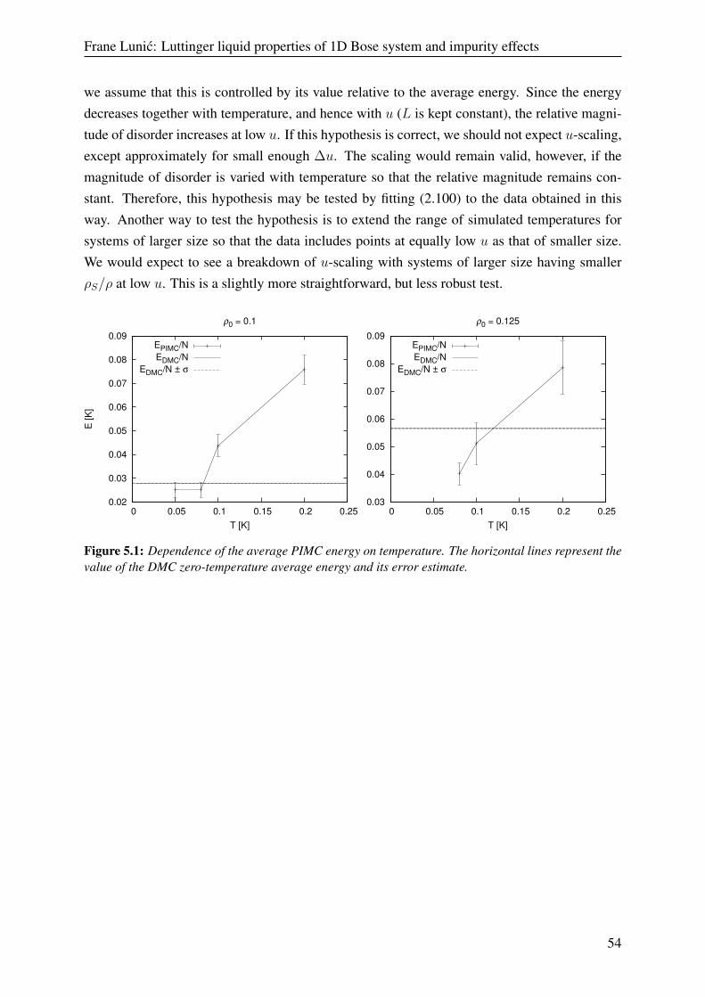
Frane Lunic: Luttinger liquid properties of 1D Bose system and impurity effects
we assume that this is controlled by its value relative to the average energy. Since the energydecreases together with temperature, and hence with u (L is kept constant), the relative magni-tude of disorder increases at low u. If this hypothesis is correct, we should not expect u-scaling,except approximately for small enough ∆u. The scaling would remain valid, however, if themagnitude of disorder is varied with temperature so that the relative magnitude remains con-stant. Therefore, this hypothesis may be tested by fitting (2.100) to the data obtained in thisway. Another way to test the hypothesis is to extend the range of simulated temperatures forsystems of larger size so that the data includes points at equally low u as that of smaller size.We would expect to see a breakdown of u-scaling with systems of larger size having smallerρS/ρ at low u. This is a slightly more straightforward, but less robust test.
0.02
0.03
0.04
0.05
0.06
0.07
0.08
0.09
0 0.05 0.1 0.15 0.2 0.25
E [
K]
T [K]
ρ0 = 0.1
EPIMC/N
EDMC/N
EDMC/N ± σ
0.03
0.04
0.05
0.06
0.07
0.08
0.09
0 0.05 0.1 0.15 0.2 0.25
T [K]
ρ0 = 0.125
EPIMC/N
EDMC/N
EDMC/N ± σ
Figure 5.1: Dependence of the average PIMC energy on temperature. The horizontal lines represent thevalue of the DMC zero-temperature average energy and its error estimate.
54
Chapter 6
Conclusion
We have studied a series of cold one-dimensional Bose systems via the worm algortihm pathintegral Monte Carlo computational method, and to an extent the diffusion Monte Carlo method.Our aim was to test the applicability of the Tomonaga-Luttinger liquid theory to these systems,especially in presence of disorder.
Our findings on systems without disorder suggest agreement with the Luttinger liquid predic-tions. Upon introducing dilute disorder, the systems show two different patterns of behaviour.The first pattern, observed in case of the largest simulated density and the Luttinger parame-ter value K < 1, is the complete cessation of u-scaling predicted by the LL model, meaningthat the superfluid fractions show separate dependence on temperature and size of the system.The superfluid fractions are not completely suppressed but since they decrease with increasingsystem size for equal u, we did not discard the possibility that the system sizes were not largeenough for localization to achieve full effect. Further research on this is needed. The secondpattern was observed in cases of the two K > 1 systems, of which at least in one, but possiblyin both cases, K was larger than 3/2. It is characterized by a u-scaling with only minor possi-ble deviations in the simulated range. The u-dependence is not well modelled by the predictedrelation, and it is not clear if this implies inapplicability of the LL model. Other possibilitiesconsidered are systematic bias and the effect of varying ratio of the average energy to the heightof the disorder-related potential barrier.
The results seem to be reconcilable with the predictions of the LL model. However, moreresearch is needed to reach firm conclusions. Tests were proposed in the discussion to verifythe convergence of large system sizes to zero superfluid fractions in K < 1 systems, and to seeif the deviations from the predicted scaling relation in K > 1 systems are due to variance in theaverage energy. Additional convergence tests should also be performed to check the quality ofsampling, optimize simulation parameters, and reduce the possibility of biased results. Asidefrom this, additional densities with more precisely determined K values should be simulatedto find the critical value of K. Systems with nondilute disorder should be simulated in order
55

Frane Lunic: Luttinger liquid properties of 1D Bose system and impurity effects
to see if this results in different a critical value, and if it corresponds to the predicted value ofKc = 3/2 for SF-BG transition in case of nondilute disorder.
56

7 Bibliography
[1] Feynman, R. P. 1972. Statistical mechanics: a set of lectures. Reading, Mass: W.A.Benjamin.
[2] Feynman, R. P. 1948. Space-time approach to non-relativistic quantum mechanics, Rev.Mod. Phys., 20 (2), 367
[3] Ceperley, D. M. 1995. Path integrals in the theory of condensed helium, Rev. Mod. Phys.67 (2), 279
[4] Coleman, A. J., Yukalov, V. I. 1992. Order indices for boson density matrices, Il NuovoCimento B, 107(5), 535
[5] Rota, R 2011., Path Integral Monte Carlo and Bose-Einstein condensation in quantum
fluids and solids (doctoral thesis), Universitat Politècnica de Catalunya
[6] Pitaevskii, L. P., Stringari, S. 2003. Bose-Einstein condensation. Oxford, UK: OxfordUniversity press
[7] Pethick, C. J., Smith, H. 2008. Bose-Einstein condensation in dilute gases (2nd ed.).Cambridge, UK: Cambridge University Press
[8] Lifshitz, E. M., Pitaevskii, L. P. 1980. Course of theoretical physics. Statistical physics,
part 2: theory of the condensed state. Oxford, United Kingdom: Pergamon
[9] Giamarchi, T. 2003. Quantum physics in one dimension. Oxford, United Kingdom:Oxford University Press
[10] Hansson, T. H. 2011. Fermi and Luttinger liquids. Lecture notes. Retrieved fromhttp://www.fysik.su.se/~hansson/cmft/notes/Fermi_Liquids.pdf
[11] Haldane, F. D. M. 1981. Effective harmonic-fluid approach to low-energy properties of
one-dimensional quantum fields. Phys. Rev. Lett. 47 (25), 1840
[12] Boninsegni, M., Prokof’ev N. V., Svistunov B.V. 2006. Worm algorithm and
diagrammatic Monte Carlo: A new approach to continuous-space path integral Monte
Carlo simulations, Phys. Rev. E 74 (3), 036701
57
Frane Lunic: Luttinger liquid properties of 1D Bose system and impurity effects
[13] Boninsegni, M. 2005. Permutation sampling in path integral Monte Carlo. J. Low Temp.Phys. 141(1-2), 27
[14] Pollock, E. L., Ceperley, D. M. 1987. Path-integral computation of superfluid densities,Phys. Rev. B 36 (16), 8343
[15] Del Maestro, A., Affleck, I. 2010. Interacting bosons in one dimension and the
applicability of Luttinger-liquid theory as revealed by path-integral quantum Monte
Carlo calculations, Phys. Rev. B 82 (6), 060515
[16] Vranješ Markic, L., Glyde, H. R. 2015. Superfluidity, BEC, and dimensions of liquid 4He
in nanopores. Phys. Rev. B 92 (6), 064510
[17] Vranješ Markic, L., Vrcan, H., Zuhrianda, Z., Glyde, H. R. 2017. Superfluidity, BEC and
the structure in 1D Luttinger liquids, manuscript submitted for publication
[18] Anderson, P. W. 1958. Absence of Diffusion in Certain Random Lattices. Phys. Rev. 109(5), 1492
[19] Cazalilla, M. A., Citro, R., Giamarchi, T. Orignac, E., Rigol, M. 2011. One dimensional
bosons: From condensed matter systems to ultracold gases Rev. Mod. Phys. 83 (4), 1405
[20] Cazalilla, M. A. 2004. Bosonizing one-dimensional cold atomic gases. J. Phys. B 37 (7),S1
[21] Giamarchi, T., Shultz, H. J. 1988. Anderson localization and interactions in
one-dimensional metals. Phys. Rev. B 37 (1), 325
[22] Ristivojevic, Z., Petkovic, A., Le Doussal, P. Giamarchi, T. 2012.Phase Transition of
Interacting Disordered Bosons in One Dimension. Phys. Rev. Lett. 109 (2), 026402
[23] Furusaki, A., Nagaosa, N. 1993 Single-barrier problem and Anderson localization in a
one-dimensional interacting electron system. Phys. Rev. B 47 (8), 4631
[24] Kane, C. L., Fisher, P. A. 1992. Transport in a one-channel Luttinger liquid. Phys. Rev.Lett. 68 (8), 1220
[25] Giamarchi, T. 2016. Quantum matter at ultralow temperatures. Book Series: Proceedingsof the International School of Physics Enrico Fermi 191, 413
[26] Gould, H., Tobochnik, J., Christian, W. 2016. An Introduction to Computer Simulation
Methods Applications to Physical System (3rd ed. revised). Retrieved from https://www.compadre.org/osp/document/ServeFile.cfm?ID=7375&DocID=527&Attachment=1
[27] Metropolis, N., Rosenbluth, A. W., Rosenbluth, M. N., Teller, A. H. 1953. Equation of
State Calculations by Fast Computing Machines. J. Chem. Phys., 21 (6), 1087
58
Frane Lunic: Luttinger liquid properties of 1D Bose system and impurity effects
[28] Doggen, E., V., H., Lemarié, G., Capponi, S., Laflorencie, N. 2017. Weak Versus Strong
Disorder Superfluid-Bose Glass Transition in One Dimension and references therein.Preprint retrieved from arXiv:1704.02257v2.
[29] Vrcan, H. 2017. Path integral Monte Carlo study of superfluid 4He in disordered narrow
nanopores (master thesis). University of Split, Faculty of Science
59