Embed Size (px)
Citation preview

PATH PLANNING FOR NONHOLONOMIC VEHICLES AND ITS APPLICATION
TO RADIATION ENVIRONMENTS
By
ARFATH PASHA
A THESIS PRESENTED TO THE GRADUATE SCHOOL OF THE UNIVERSITY OF FLORIDA IN PARTIAL FULFILLMENT
OF THE REQUIREMENTS FOR THE DEGREE OF MASTER OF SCIENCE
UNIVERSITY OF FLORIDA
2003

Copyright 2003
by
Arfath Pasha

I dedicate this thesis to my mother. The quality education that I have received is a result of her perseverance.

ACKNOWLEDGMENTS
To the members of my committee, Dr. Carl Crane, Dr. Ashok Kumar and
Professor Tulenko, I would like to extend my thanks. To Dr. Crane for mentoring me
through five years and two degrees, for his confidence in allowing me to undertake some
of the most fascinating projects at CIMAR, I owe my grateful thanks.
Dr. Dalton’s knowledge on nuclear physics has been crucial to my project. I thank
Donald MacArthur and Erica Zawodny for venturing to put to test the path planner in a
real world situation. I thank Marinela Capanu my companion who has offered her
unwavering support and long brainstorming sessions despite her hectic schedule. Finally,
I thank Carol Chesney for her help during the final phase of the thesis.
iv
TABLE OF CONTENTS Page ACKNOWLEDGMENTS ................................................................................................. iv
LIST OF FIGURES .......................................................................................................... vii
ABSTRACT.........................................................................................................................x
CHAPTER 1 INTRODUCTION AND BACKGROUND .................................................................1
Problem Statement........................................................................................................1 Kinematic Constraints of Car-Like Robots ..................................................................2 Path Planning Algorithms.............................................................................................3 Offline Path Planning for Car-Like Vehicles ...............................................................4 Need for a Path Planner in Radiation Environments ....................................................6 Effects of Radiation on Mobile Robots ........................................................................7
2 LITERATURE SURVEY.............................................................................................9
Theoretical Work ..........................................................................................................9 Non-Deterministic Approaches ..................................................................................11 Deterministic Approaches ..........................................................................................13
3 RESEARCH OBJECTIVES.......................................................................................17
Formal Problem Statement: Path Planner...................................................................17 Formal Problem Statement: Path Planner with a Radiation Constraint......................21
4 NON-HOLONOMIC PATH PLANNING ALGORITHM ........................................22
Pre-Process .................................................................................................................22 Input Validation...................................................................................................22 Pre-Computation..................................................................................................23
Obstacle Expansion ....................................................................................................24 Expansion of Convex Obstacle Vertices .............................................................29 Expansion of Concave Obstacle Vertices............................................................30 Main Result: Expansion Method Guarantees Admissible Trajectories...............32
Visibility Graph ..........................................................................................................40 Shortest Path ...............................................................................................................42
v
5 PATH PLANNING WITH A RADIATION CONSTRAINT....................................44
Radiation Basics .........................................................................................................44 Algorithm Description ................................................................................................46
6 RESULTS AND CONCLUSION...............................................................................54
APPENDIX A ATTENUATION........................................................................................................62
B DATA STRUCTURE.................................................................................................65
LIST OF REFERENCES...................................................................................................89
BIOGRAPHICAL SKETCH .............................................................................................92
vi

LIST OF FIGURES
Figure page 1-1 Geometry of a car-like vehicle ...................................................................................2
1-2 Configuration space for a disc robot. .........................................................................5
2-1 Dubin’s Shortest paths for a particle with a minimum radius of curvature constraint.10
2-2 Reeds and Shepp’s Shortest paths for a car moving both forward and backward. ..10
2-3 Output of a probabilistic path planner developed by Laumond et al. [10]. (a) An initial holonomic path (b-d) Optimization of the nonholonomic path. ....................12
2-4 An output of a randomized algorithm developed by Bessiere et al. [13].................13
2-5 Visibility graph of a map..........................................................................................14
2-6 Center-line paths developed by Suh and Shin [22] ..................................................16
3-1 Minimum angle constraint on concave vertices of polygons. ..................................18
3-2 Constraint on edge lengths for the vehicle to brace the obstacle. ............................19
4-1 Flowchart of the nonholonomic path planner. .........................................................23
4-2 Graphic representation of program flow. .................................................................24
4-3 Geometry of a pseudo obstacle placed around the vehicle’s start configuration. ....25
4-4 A clothoid (Cornu spiral). ........................................................................................26
4-5 Paths smoothed with clothoid curves [24]. ..............................................................26
4-6 Polynomial curve suggested by the JAUS Reference Architecture [25] for the generation of a trajectory..........................................................................................27
4-7 Effect of the weighting w factor on the trajectory....................................................28
4-8 A trajectory made up of two curve segments that share a common tangent. ...........28
4-9 Geometry of expansion of a convex obstacle vertex................................................30
vii
4-10 Boundary conditions for the expansion of convex obstacle vertices. ......................30
4-11 Geometry of expansion of a concave obstacle vertex. .............................................31
4-12 Boundary conditions for the expansion of concave obstacle vertices......................31
4-13 The worst case turn. .................................................................................................33
4-14 Plot of curvature κ versus parameter u for a symmetric curve with w = 0.707 .......34
4-15 Violation of the assumption on minimum path segment length l0. ..........................35
4-16 A problem instance where the assumption on minimum path segment length l0 is violated. ....................................................................................................................36
4-17 The worst case turn for the special case. ..................................................................37
4-18 Plot of curvature κ versus parameter u for the special case with w = 0.875............38
4.19 A problem instance where two or more consecutive path segments have lengths less than l0.................................................................................................................39
4-20 The worst case scenario when the path is smoothed. ...............................................39
4-21 Radial sweep method used to find the visibility of vertices.....................................41
4-22 Determining the visibility of vertices.......................................................................43
5-1 A point source of radiation.......................................................................................46
5-2 Optimal paths in a map with no boundary. ..............................................................47
5-3 Growing pseudo obstacles around radiation sources to find an optimal path. .........49
5-4 Radiation sources placed parallel with respect to a path between the start and goal points. .......................................................................................................................50
5-5 A case with a constricting pseudo obstacle. .............................................................51
5-6 Flow chart of the path planner with a radiation constraint.......................................52
6-1 Shortest path in a map with non-convex obstacles and a boundary.........................55
6-2 An admissible trajectory for the path generated in Figure 6-1.................................56
6-3 A special case when the length of a path segment is less than l0. ............................56
6-4 An admissible trajectory for the path generated in Figure 6-3.................................57
viii
6-5 A trivial case of a straight line path..........................................................................57
6-6 A case where concave boundary vertices are used to find a path. ...........................58
6-7 An admissible trajectory for the path generated in Figure 6-6.................................58
6-8 A radiation environment with no boundary. ............................................................59
6-9 A bounded radiation environment............................................................................59
6-10 Another bounded radiation environment..................................................................60
6-11 A case where a zero dose path does not exist...........................................................60
6-12 A case with a constricting pseudo obstacle. .............................................................61
6-13 Path planner used for online path planning. .............................................................61
A-1 Attenuation from a plane shield in front of a point source of radiation. ..................62
A-2 Radial sweep line method to compute attenuation...................................................64
B-1 Code layout. .............................................................................................................65
ix
Abstract of Thesis Presented to the Graduate School
of the University of Florida in Partial Fulfillment of the Requirements for the Degree of Master of Science
PATH PLANNING FOR NONHOLONOMIC VEHICLES AND ITS APPLICATION TO RADIATION ENVIRONMENTS
By
Arfath Pasha
August 2003
Chair: Carl D. Crane III Major Department: Mechanical and Aerospace Engineering
Mobile robots are often used in hazardous work places such as nuclear power
plants. Although the use of robots in such environments minimizes the danger of
radiation exposure to humans, the robots themselves are susceptible to damage from
radiation. In order to minimize the amount of radiation they receive, an efficient path-
planning algorithm was developed for autonomous mobile robots with nonholonomic
constraints and modified to find safe paths in radiation environments. The objective of
the algorithm was to find a reasonably close approximation to the safest path from a
given start configuration to a goal configuration of a vehicle moving only forward in an
environment cluttered with obstacles bounded by simple polygons. The path planning
algorithm finds the shortest path in O(n2logn) time (n being the number of vertices in the
discretized map) using a radial sweep line method to compute the visibility graph and
Dijkstra's algorithm to find the shortest path.
x
CHAPTER 1 INTRODUCTION AND BACKGROUND
Motion planning is one of the most important components of an autonomous
mobile vehicle. It deals with the search and execution of collision free paths by vehicles
performing specific tasks. Motion planning is often broken down into two stages--path
planning and path tracking. The path planning stage involves the search for a collision
free path, taking into consideration the geometry of the vehicle and it surroundings, the
vehicle's kinematic constraints and any other external constraints that may affect the
planning of a path. The path tracking stage involves the actual navigation of a planned
path, taking into consideration the kinematic and dynamic constraints of the vehicle. This
research presents a path planning algorithm for car-like vehicles.
Problem Statement
The objective of this effort is two fold:
1. To develop an efficient offline path planning algorithm that is capable of finding optimal collision free paths from a start point to a goal, for a car-like vehicle moving through an environment containing obstacles bounded by simple polygons.
2. To extend the path planning algorithm in order to find safe paths by imposing a radiation constraint on a mobile robot operating in a radiation environment.
The first objective was intended to be an improvement of the work done by Arturo
Rankin [1]. The second objective was intended to facilitate the optimal utilization of
robotic vehicles in places such as nuclear power plants where prolonged exposure to
radiation can cause substantial damage to robotic equipment.
1
2
Kinematic Constraints of Car-Like Robots
The motion characteristics of a robot play an important role in planning its path.
Robots that move in a plane generally have three degrees of freedom--translation along
the two axes in the plane and rotation about the axis perpendicular to the plane. Certain
robots that are car-like cannot move freely in all three degrees of motion due to their
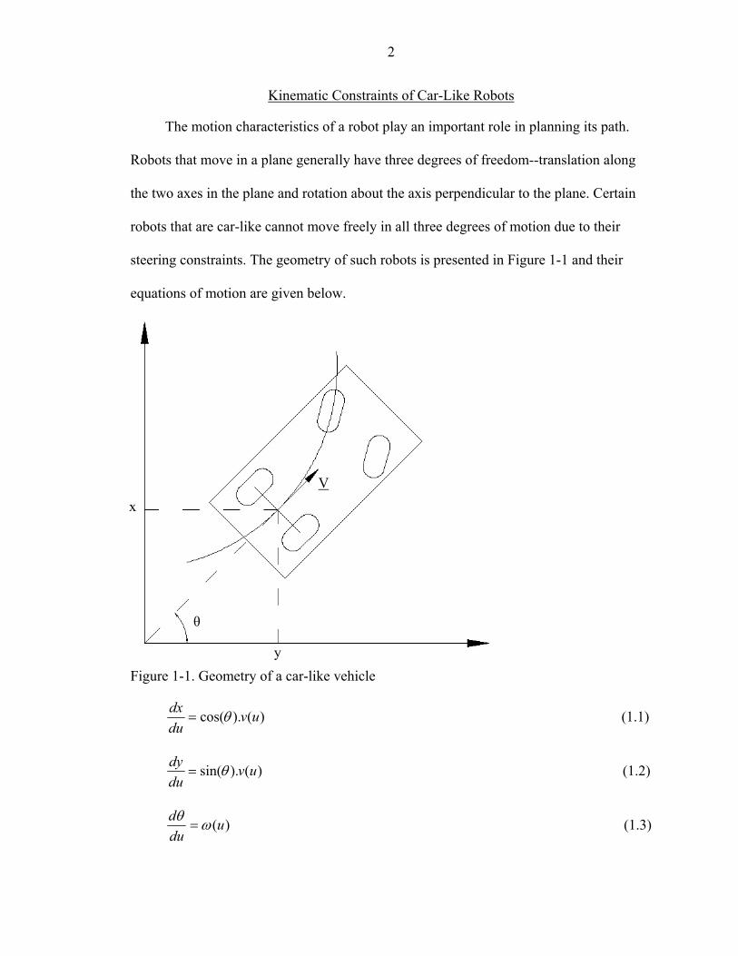
steering constraints. The geometry of such robots is presented in Figure 1-1 and their
equations of motion are given below.
Vx
θ
y Figure 1-1. Geometry of a car-like vehicle
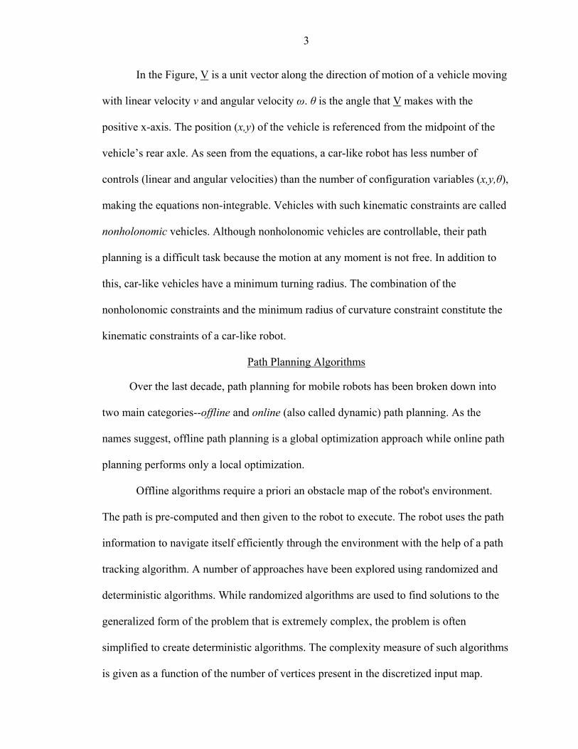
)().cos( uvdudx θ= (1.1)
)().sin( uvdudy θ= (1.2)
)(udud ωθ
= (1.3)
3
In the Figure, V is a unit vector along the direction of motion of a vehicle moving
with linear velocity v and angular velocity ω. θ is the angle that V makes with the
positive x-axis. The position (x,y) of the vehicle is referenced from the midpoint of the
vehicle’s rear axle. As seen from the equations, a car-like robot has less number of
controls (linear and angular velocities) than the number of configuration variables (x,y,θ),
making the equations non-integrable. Vehicles with such kinematic constraints are called
nonholonomic vehicles. Although nonholonomic vehicles are controllable, their path
planning is a difficult task because the motion at any moment is not free. In addition to
this, car-like vehicles have a minimum turning radius. The combination of the
nonholonomic constraints and the minimum radius of curvature constraint constitute the
kinematic constraints of a car-like robot.
Path Planning Algorithms
Over the last decade, path planning for mobile robots has been broken down into
two main categories--offline and online (also called dynamic) path planning. As the
names suggest, offline path planning is a global optimization approach while online path
planning performs only a local optimization.
Offline algorithms require a priori an obstacle map of the robot's environment.
The path is pre-computed and then given to the robot to execute. The robot uses the path
information to navigate itself efficiently through the environment with the help of a path
tracking algorithm. A number of approaches have been explored using randomized and
deterministic algorithms. While randomized algorithms are used to find solutions to the
generalized form of the problem that is extremely complex, the problem is often
simplified to create deterministic algorithms. The complexity measure of such algorithms
is given as a function of the number of vertices present in the discretized input map.

4
The main objective of online path planning is to avoid obstacles by reacting to
data collected from onboard sensors. It may be used when a map of the mobile robot's
environment is not known or, if an unexpected obstacle was encountered during the
execution of a pre-computed path. Since online path planners run in real time and on
onboard computers that usually have very limited computing resources, they have to be
efficient in terms of both memory utilization and time. This is accomplished by using a
lightweight algorithm or heuristic that works on a highly discretized input. Their
efficiency is usually measured by the amount of time they take. The quality of their
results depends on the amount of look-ahead distance of the sensors. Path length is
usually used as a complexity measure for online path planning algorithms by setting
bounds for the worst case path length as a function of environmental parameters such as
the sum of perimeter lengths of obstacles [2].
A natural offshoot from creating a distinction between online and offline
algorithms is the development of hybrid algorithms. Hybrid path planning algorithms
usually work with sparse or low resolution maps that do not provide information about
obstacles such as rocks, trees etc. These algorithms have both an online and an offline
component that work in tandem to provide globally optimal paths.
Offline Path Planning for Car-Like Vehicles
The generalized offline path planning problem for car-like robots is referred to as
the continuous curvature constrained shortest path problem. The objective of the
generalized problem is to find a continuous path that is the shortest among all paths and
whose curvature at any point along the path is less than a given upper bound (the inverse
of the minimum turning radius). Reif and Wang [3] proved that this problem is NP-hard.
This means that there is no existing algorithm that can solve this problem to optimality in
5
polynomial time and it is highly unlikely that one even exists; a justification for the
approaches based on discretization used in the past to yield polynomial time algorithms.
Fortunately, these approaches have been found to work well for all practical applications.
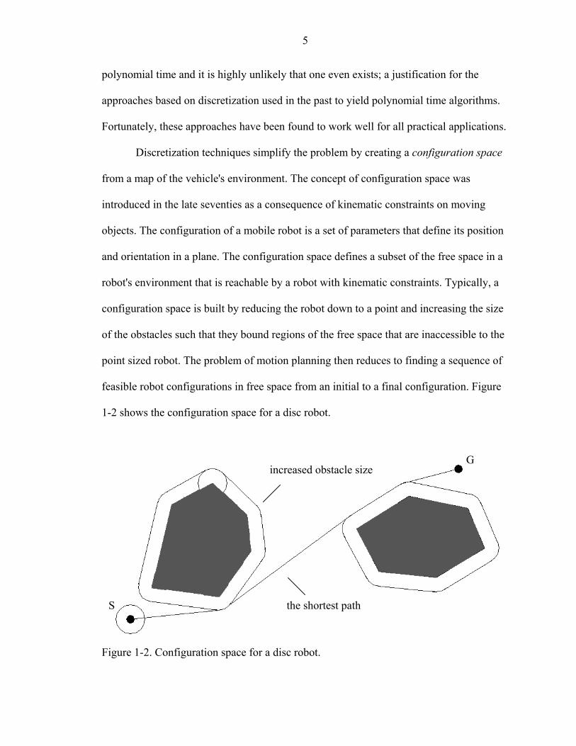
Discretization techniques simplify the problem by creating a configuration space
from a map of the vehicle's environment. The concept of configuration space was
introduced in the late seventies as a consequence of kinematic constraints on moving
objects. The configuration of a mobile robot is a set of parameters that define its position
and orientation in a plane. The configuration space defines a subset of the free space in a
robot's environment that is reachable by a robot with kinematic constraints. Typically, a
configuration space is built by reducing the robot down to a point and increasing the size
of the obstacles such that they bound regions of the free space that are inaccessible to the
point sized robot. The problem of motion planning then reduces to finding a sequence of
feasible robot configurations in free space from an initial to a final configuration. Figure
1-2 shows the configuration space for a disc robot.
Gincreased obstacle size
S the shortest path
Figure 1-2. Configuration space for a disc robot.

6
The planned path is considered to be an image of the final trajectory that is
executed by the robot. The path may be discontinuous but the trajectory is always
continuous. An admissible trajectory is a solution of the differential system
corresponding to the kinematic model of the robot along with some initial and final
conditions. Since the configuration space concept is purely geometric and does not allow
for time-dependant constraints (as required by the robot's kinematic model) the goal of a
discretized nonholonomic path planner is to find an image of an admissible trajectory--a
collision free admissible path.
Need for a Path Planner in Radiation Environments
Robots are used in nuclear installations to perform jobs in areas where humans are
at risk of being over exposed to radiation. Since radiation is detrimental to human health,
the amount of access that humans have to portions of an installation is limited by
regulation 10CFR20 of the Nuclear Regulatory Commission [4]. This limitation may call
for the need to employ more labor than needed.
In addition to this, there are as many as 7000 contaminated buildings among
Department of Energy nuclear facilities that require decontamination and/or
decommissioning. It is estimated that it will take more than 40 years and over 100 billion
dollars to clean up these sites [5]. The Department of Energy: Office of Environmental
Management, set up a program called the "CP-5 Large Scale Demonstration Project" [6]
to find innovative decontamination and decommissioning technologies that can help
reduce the cost of this billion dollar effort. Some of the solutions that were developed
were radiation imaging systems that could map radiation fields and mobile robots that
were capable of finding hotspots in a building. Since robots themselves are affected by
radiation and the cost of maintaining or replacing them is high, significant cost savings

7
can be achieved by minimizing their exposure to radiation. One way of doing this is by
using a path planner to compute routes that minimize the radiation exposure of mobile
robots and thereby extending their life.
Effects of Radiation on Mobile Robots
Gamma rays, beta particles, neutrons and heavy charged particles such as protons
and alpha particles are emitted from radioactive materials. Of these, gamma rays, which
are photons with very short wave length, pose the greatest threat to electrical and
electronic components onboard robots. Gamma radiation is capable of traveling many
meters in air and readily penetrates most material, earning itself the name "penetrating
radiation." Gamma rays have a very destructive effect on a number of materials used to
build robots. Electrical parts such as transformers, motors, thermocouples, relays and
circuit boards, which form vital components of a robot may be severely damaged from
exposure to gamma radiation. Laurent Houssay [7] has detailed the effects of gamma rays
and has referenced tables with threshold values for various materials that are used on
robotic systems. The effect of radiation from gamma rays is increased by long exposure
(time), close proximity to its source (distance) and the intensity of the source (quantity).
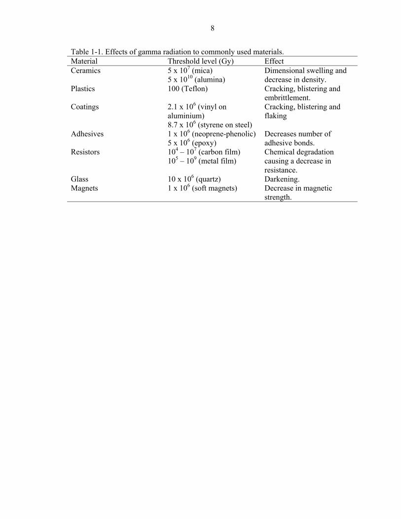
Some effects of gamma radiation on commonly used materials are listed in table 1-1.
8
Table 1-1. Effects of gamma radiation to commonly used materials. Material Threshold level (Gy) Effect Ceramics 5 x 10⁷ (mica)
5 x 10¹⁰ (alumina) Dimensional swelling and decrease in density.
Plastics 100 (Teflon) Cracking, blistering and embrittlement.
Coatings 2.1 x 10⁶ (vinyl on aluminium) 8.7 x 10⁶ (styrene on steel)
Cracking, blistering and flaking
Adhesives 1 x 10⁶ (neoprene-phenolic) 5 x 10⁶ (epoxy)
Decreases number of adhesive bonds.
Resistors 104 – 107 (carbon film) 105 – 109 (metal film)
Chemical degradation causing a decrease in resistance.
Glass 10 x 106 (quartz) Darkening. Magnets 1 x 10⁶ (soft magnets) Decrease in magnetic
strength.
CHAPTER 2 LITERATURE SURVEY
This section summarizes previous research work done in offline path planning for
nonholonomic mobile robots. A significant amount of work has been done in both
theoretical analysis of the problem and the development of algorithms for finding
effective solutions for planning globally optimal paths.
Theoretical Work
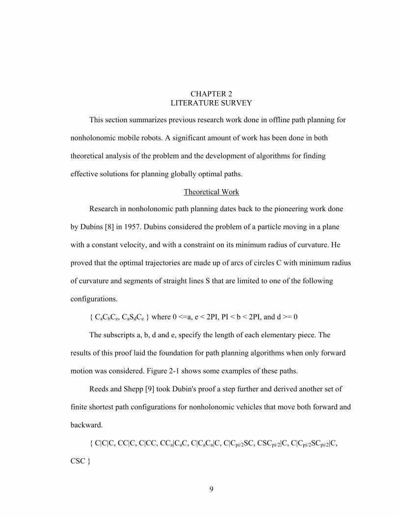
Research in nonholonomic path planning dates back to the pioneering work done
by Dubins [8] in 1957. Dubins considered the problem of a particle moving in a plane
with a constant velocity, and with a constraint on its minimum radius of curvature. He
proved that the optimal trajectories are made up of arcs of circles C with minimum radius
of curvature and segments of straight lines S that are limited to one of the following
configurations.
{ CaCbCe, CaSdCe } where 0 <=a, e < 2PI, PI < b < 2PI, and d >= 0
The subscripts a, b, d and e, specify the length of each elementary piece. The
results of this proof laid the foundation for path planning algorithms when only forward
motion was considered. Figure 2-1 shows some examples of these paths.
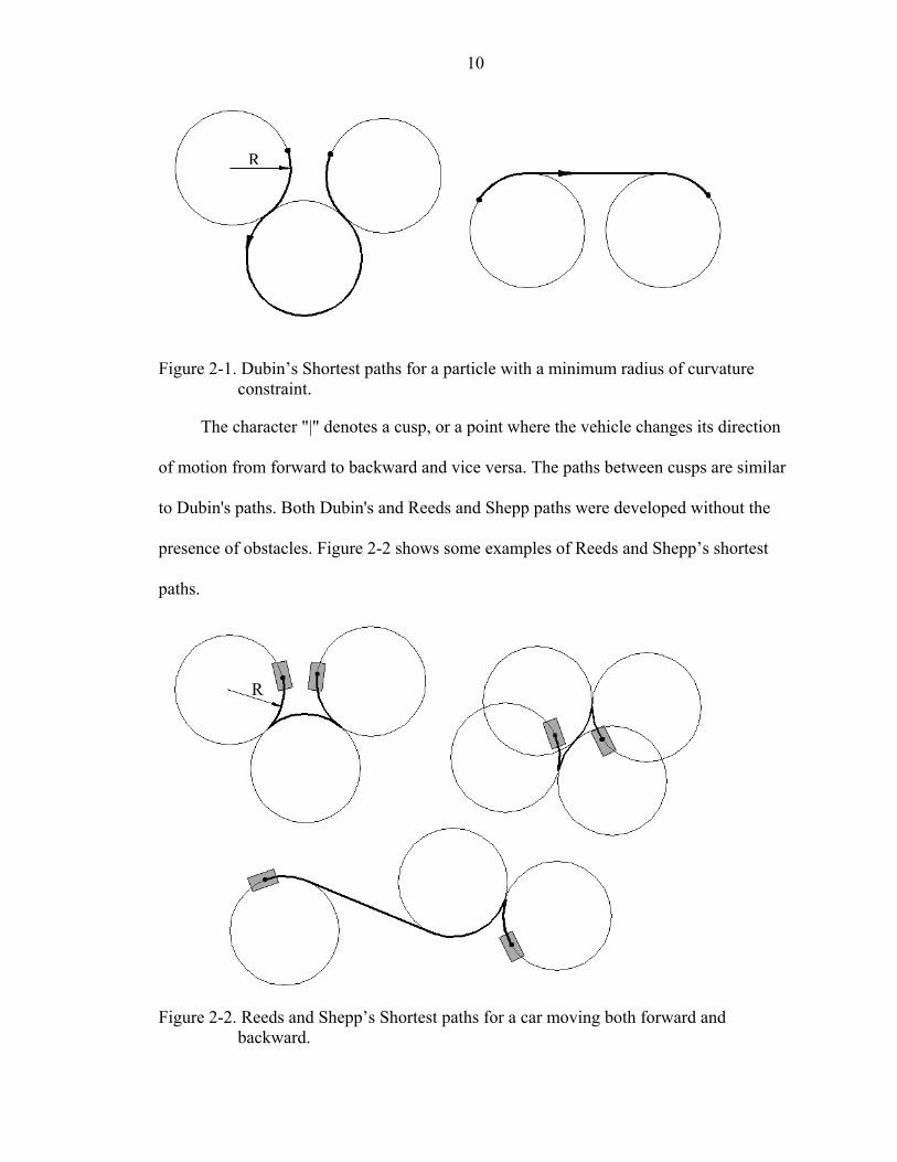
Reeds and Shepp [9] took Dubin's proof a step further and derived another set of
finite shortest path configurations for nonholonomic vehicles that move both forward and
backward.
{ C|C|C, CC|C, C|CC, CCa|CaC, C|CaCa|C, C|Cpi/2SC, CSCpi/2|C, C|Cpi/2SCpi/2|C,
CSC }
9
10
Figure 2-1. c
The c
of motion fr
to Dubin's p
presence of
paths.
Figure 2-2. b
R
Dubin’s Shortest paths for a particle with a minimum radius of curvature onstraint.
haracter "|" denotes a cusp, or a point where the vehicle changes its direction
om forward to backward and vice versa. The paths between cusps are similar
aths. Both Dubin's and Reeds and Shepp paths were developed without the
obstacles. Figure 2-2 shows some examples of Reeds and Shepp’s shortest
R
Reeds and Shepp’s Shortest paths for a car moving both forward and ackward.
11
Using these finite family of curves, it is simple to design an algorithm to find the
shortest path between any two configurations. But, the presence of obstacles and the fact
that a mobile vehicle needs a continuous path to be able to follow it accurately made such
a solution impractical. Obstacles make the search difficult by limiting the number of
admissible robot placements. Dubin's configurations guaranteed shortest paths for mobile
vehicles with curvature constraints, but the configurations are discontinuous at the points
where two elementary components are connected. A vehicle that attempts to follow these
paths must come to a complete stop at these points to align its steering with the (tangent
in case of an arc) direction of the next segment in order to follow these paths accurately.
Such motions are undesirable.
Finding shortest paths with continuous curvature came to be known as the
generalized offline path planning problem for car-like robots. It is a difficult task even
with the absence of obstacles and remained an open problem for a number of years until
it was proved to be NP-Hard by Reif and Wang [3] in 1998.
Non-Deterministic Approaches
A few attempts that used probabilistic methods and randomized algorithms were
used to develop algorithms for the generalized path planning problem. Probabilistic path
planners (PPP) are guaranteed to solve a problem for which a solution exists within
infinite time. That is, as the running time of the algorithm goes to infinity, the probability
of solving it converges to one. In some cases, a guaranteed probability value of reaching
the optimal solution is given for reasonable (polynomial) running times. Just as in the
case of PPP, randomized path planners (RPP) can also be proven to have a guaranteed
probability of reaching an optimal solution in polynomial time. The difference in the two
methods arise from the technique used to solve the problem. PPP algorithms use iterative
12
procedures that perform neighborhood walks to find an optimal solution, while RPP
algorithms use random walks through the solution space to find an optimal solution.
PPP algorithms are typically broken down into two or more stages. The first stage
checks if the problem is solvable (a decision problem). If the problem is found to be
solvable, the second stage finds an approximate solution, which is then optimized by the
third stage that uses an iterative search method. A good example of a PPP is given by
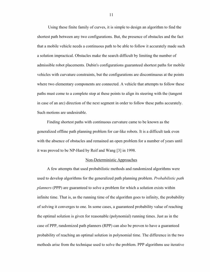
Laumond et al. [10]. Their work uses a holonomic path planner to find a path of minimal
length. The minimum length path is then approximated to a nonholonomic path using
Reeds and Shepp's finite set of shortest paths. The approximated path is then optimized
iteratively in the final stage of the algorithm. Figure 2-3 shows the stages of this
algorithm. Similar methods have been tried by Lafferriere and Sussman [11] and Jacob
[12].
(a) (b)
(c) (d)Figure 2-3. Output of a probabilistic path planner developed by Laumond et al. [10]. (a)
An initial holonomic path (b-d) Optimization of the nonholonomic path.
13
RPP algorithms are somewhat similar to PPP in the sense that this method also
involves two or more search stages. RPPs typically use randomized heuristics such as
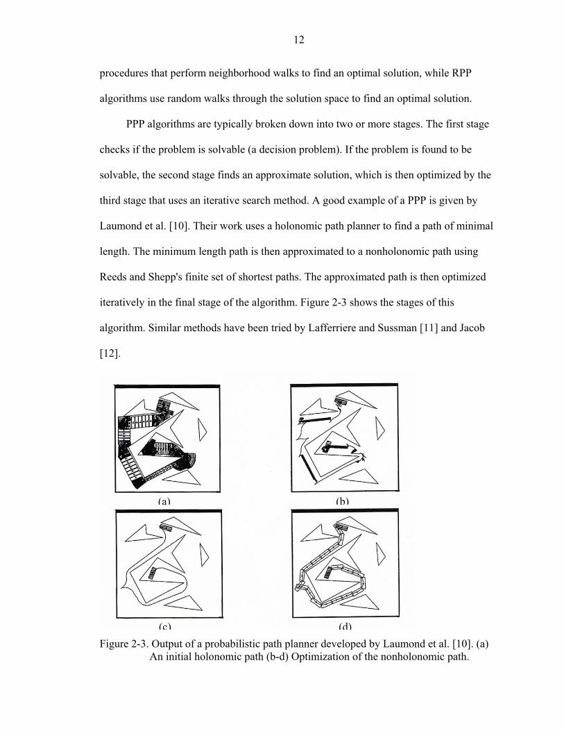
simulated annealing and genetic algorithms. Bessiere et al. [13] have developed one such
technique that has two stages--search and explore. The search stage finds if it is possible
to "simply" reach the goal. The explore stage collects information about the environment
and optimizes the path found in the search stage by using landmarks placed all over the
environment. Exploration of the environment is done with the help of a genetic
algorithm. Figure 2-4 shows an output of their algorithm.
Figure 2-4. An output of a randomized algorithm developed by Bessiere et al. [13].
Deterministic Approaches
The bulk of the path planners designed for nonholonomic motion over the last
decade make certain assumptions to help simplify the problem down to a more tractable
14
one. This has allowed the use of simple and efficient heuristic type solutions to tackle
practical problems at considerably low running times. The most popular of these
assumptions is to assume that an admissible trajectory can be obtained from a
discontinuous collision free path made up of straight-line segments and circular arcs of
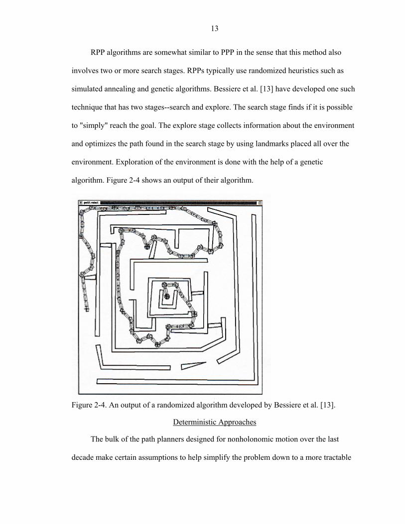
bounded curvature. A well tried and tested method that was first introduced by Perez and
Wesley [14] is the visibility graph search method. This method reduces the obstacle map
along with the start and goal points down to a graph structure where the visibility of each
node (vertices of obstacles) with respect to other nodes in the graph is computed. The
shortest path is built by connecting visible nodes beginning from the start node and
ending with the goal node. The straight lines in Figure 2-5 represent the visibility lines
S
GFigure 2-5. Visibility graph of a map.
from each node to every other visible node in the graph. Graph based algorithms such as
A* search [15], Dijkstra's, Bellman-Ford and Floyd-Warshall algorithms [16] may be
applied to the resulting visibility graph to find the shortest paths. Researchers that have
used this technique include Bicchi et al. [17], Rankin [1] and Asano et al. [18].
15
There has also been a host of other deterministic methods that have been developed
for a simplified version of the problem. Among them, Namgung and Duffy [19] proposed
a new idea of using linear parametric curves to find collision free paths. Their method
built an initial discontinuous collision free path that was later smoothed at the
discontinuities to yield a continuous path. The continuous path was guaranteed to lie in
free space after the smoothing operation was performed. Another approach called cell
decomposition, was first developed by Brooks and Perez [20]. It consists of decomposing
the configuration space into rectangular cells that lie in free space, and then planning a
path as a sequence of empty cells (cells lying in free space). Many improvements have
been made using this approach. One such improvement is the hierarchical cell
decomposition approach presented by Zhu and Latombe [21].
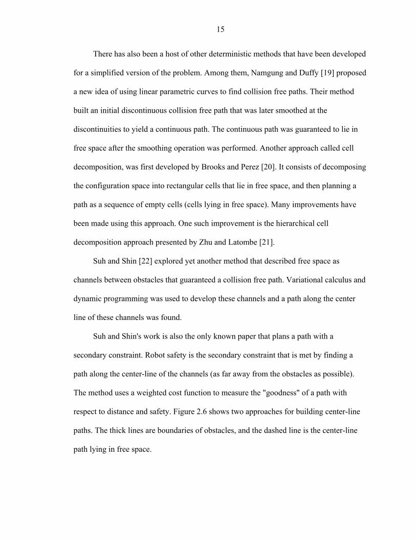
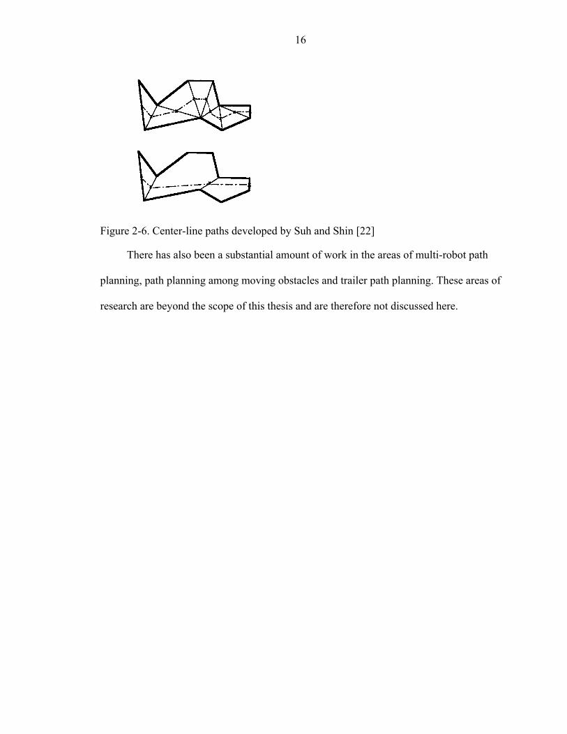
Suh and Shin [22] explored yet another method that described free space as
channels between obstacles that guaranteed a collision free path. Variational calculus and
dynamic programming was used to develop these channels and a path along the center
line of these channels was found.
Suh and Shin's work is also the only known paper that plans a path with a
secondary constraint. Robot safety is the secondary constraint that is met by finding a
path along the center-line of the channels (as far away from the obstacles as possible).
The method uses a weighted cost function to measure the "goodness" of a path with
respect to distance and safety. Figure 2.6 shows two approaches for building center-line
paths. The thick lines are boundaries of obstacles, and the dashed line is the center-line
path lying in free space.
16
Figure 2-6. Center-line paths developed by Suh and Shin [22]
There has also been a substantial amount of work in the areas of multi-robot path
planning, path planning among moving obstacles and trailer path planning. These areas of
research are beyond the scope of this thesis and are therefore not discussed here.
CHAPTER 3 RESEARCH OBJECTIVES
Formal Problem Statement: Path Planner
Given:
1. The start and goal configurations (xs,ys,θs) and (xg,yg,θg) of a car-like robot in a plane;
2. Dimensions of the robot--length L, width W, minimum turning radius R; 3. A collection O = {o1, o2,…,on} of non overlapping obstacles described by simple
polygons, each having a set of vertices Vi = {vij , j = 1, …, mi }, i = 1, …, n, and such that the length of each edge is at least l0 and the angle subtended at each concave vertex is in the range [π/2, π]. (Note that O can be the empty set.)
4. A set of vertices B = {b1, b2, …, bN} describing a simple polygon that defines a boundary such that the length of each edge is at least l0 and the angle subtended at each convex vertex is in the range [π/2, π]. (Note that B can also be the empty set.)
Find:
A set of way points P = {P1, …., Pk}starting with the start position and ending with the goal position, that is an image of an admissible trajectory of minimal distance for a robot moving only forward.
The input universe for each of the inputs mentioned above were made as general as
possible to allow maximum flexibility. But, some constraints had to be imposed in order
to guarantee a collision free admissible path. These constraints arise mainly from the
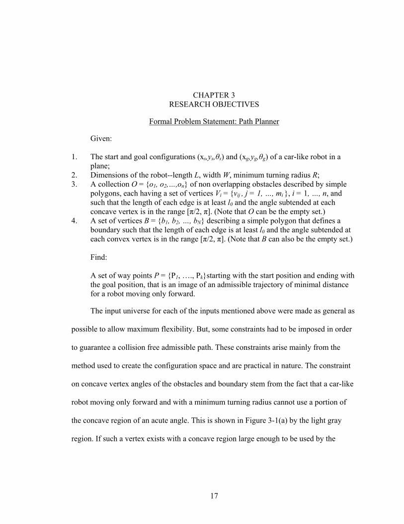
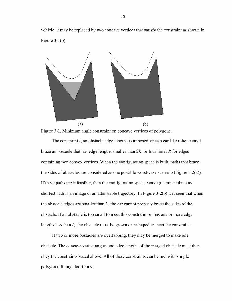
method used to create the configuration space and are practical in nature. The constraint
on concave vertex angles of the obstacles and boundary stem from the fact that a car-like
robot moving only forward and with a minimum turning radius cannot use a portion of
the concave region of an acute angle. This is shown in Figure 3-1(a) by the light gray
region. If such a vertex exists with a concave region large enough to be used by the
17
18
vehicle, it may be replaced by two concave vertices that satisfy the constraint as shown in
Figure 3-1(b).
(a) (b) Figure 3-1. Minimum angle constraint on concave vertices of polygons.
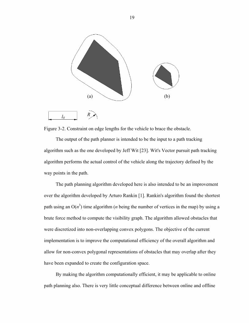
The constraint l0 on obstacle edge lengths is imposed since a car-like robot cannot
brace an obstacle that has edge lengths smaller than 2R, or four times R for edges
containing two convex vertices. When the configuration space is built, paths that brace
the sides of obstacles are considered as one possible worst-case scenario (Figure 3.2(a)).
If these paths are infeasible, then the configuration space cannot guarantee that any
shortest path is an image of an admissible trajectory. In Figure 3-2(b) it is seen that when
the obstacle edges are smaller than l0, the car cannot properly brace the sides of the
obstacle. If an obstacle is too small to meet this constraint or, has one or more edge
lengths less than l0, the obstacle must be grown or reshaped to meet the constraint.
If two or more obstacles are overlapping, they may be merged to make one
obstacle. The concave vertex angles and edge lengths of the merged obstacle must then
obey the constraints stated above. All of these constraints can be met with simple
polygon refining algorithms.
19
(a) (b)
R l0
Figure 3-2. Constraint on edge lengths for the vehicle to brace the obstacle.
The output of the path planner is intended to be the input to a path tracking
algorithm such as the one developed by Jeff Wit [23]. Wit's Vector pursuit path tracking
algorithm performs the actual control of the vehicle along the trajectory defined by the
way points in the path.
The path planning algorithm developed here is also intended to be an improvement
over the algorithm developed by Arturo Rankin [1]. Rankin's algorithm found the shortest
path using an O(n3) time algorithm (n being the number of vertices in the map) by using a
brute force method to compute the visibility graph. The algorithm allowed obstacles that
were discretized into non-overlapping convex polygons. The objective of the current
implementation is to improve the computational efficiency of the overall algorithm and
allow for non-convex polygonal representations of obstacles that may overlap after they
have been expanded to create the configuration space.
By making the algorithm computationally efficient, it may be applicable to online
path planning also. There is very little conceptual difference between online and offline
20
path planning. Both seek optimal paths from a start to a goal. Online path planners work
on local data while offline path planners work on global data. Theoretically, an online
path planner may be used for offline path planning and vice versa. The main difference
that does not permit this interchange stems from the practical issues of computational
efficiency, scalability and nature of the input. Offline path planners are not fast enough to
run in real time while online algorithms are not built to be scalable. Online planners work
on range data collected from sensors while offline planners work on discretized map data.
By developing an offline algorithm that is computationally efficient enough to run in real
time, it may also be applied to online path planning with an added overhead of converting
the input into a discretized local map.
By generalizing the obstacle input to include non-convex polygons, more accurate
representations of the obstacles may be used. Also, when the configuration space is built,
the size of the obstacles is increased in order to reduce the robot to a point in the map.
Increasing the size of the obstacles can cause the expanded obstacles to overlap. Such
intersections are permitted by the current implementation.
The boundary polygon was included into the input in order to be able to define a
closed working space for the robot. This can be particularly useful in certain online path
planning applications such as path following, and for path planning in radiation
environments. When the boundary is specified, the edges of the boundary are shrunk in a
manner similar to the expansion of the obstacles. The boundary vertices when specified
are used in the construction of the visibility graph and hence the shortest path algorithm.
The input set of vertices for the boundary may be an empty set when the boundary is not
specified.
21
Formal Problem Statement: Path Planner with a Radiation Constraint
In addition to the inputs mentioned in the formal problem statement of the path planner,
Given:
5. The maximum speed of the vehicle vmax; 6. A set of radiation sources G = {G1, ..., Gr}with positions (xi, yi), and dose rates Ii,
i = 1,., r.
Find:
A set of way points P = {P1, ..., Pk}starting with the start position and ending with the goal position, that is an image of an admissible trajectory of minimal distance for a robot moving only forward, such that the dose, Ic accumulated by the robot along the path is minimal.
The objective of this part of the problem is to incorporate the new radiation
constraint by building on the basic path planner. An important issue to consider is that the
algorithm must optimize against two unrelated constraints--distance and radiation
absorption or dose. A popular approach to solving such problems is to devise a weighted
cost function as done by Suh and Shin [22] that may have an inherent mixed units
problem. The approach used here avoids the mixed units problem by minimizing the
accumulated dose independent of distance. It is assumed that the radiation sources are
point sources and that the accumulated dose is the sum total of dose received from all
sources present in the robot's environment.
CHAPTER 4 NON-HOLONOMIC PATH PLANNING ALGORITHM
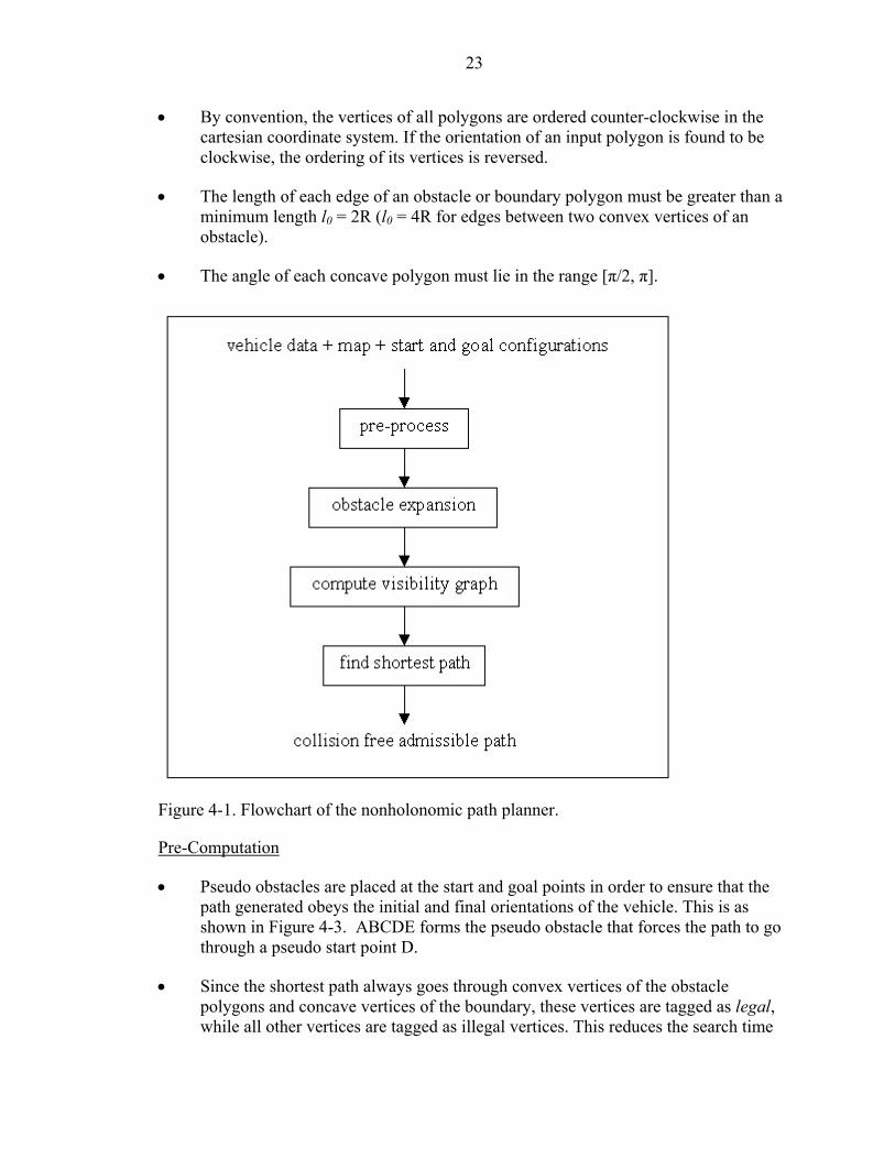
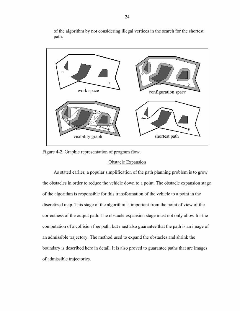
The algorithm for planning of a collision free admissible path was broken down
into four stages as shown in Figure 4-1 and 4.2. The algorithm is built on an edge-centric
data structure that is listed in Appendix B. All points in the map are referenced to a
cartesian coordinate system (x,y). The boundary polygon is treated as the inverse of the
obstacle polygon. That is, the final trajectory must be contained by the boundary polygon
while lying outside the obstacle polygons. If the operations on the boundary polygon are
not explicitly stated, they must be considered as the inverse of the operations performed
on the obstacle polygons wherever appropriate.
Pre-Process
The pre-process stage of the algorithm validates the input and performs some pre-
computation that helps in speeding up the main body of the algorithm. The lists below,
detail the validation and pre-computations that are performed on the input. Failure of any
of the validity checks may lead to the premature termination of the algorithm.
Input Validation
• Check for non-empty start and goal configurations that lie in free space. That is, the configurations must exist in the input and the position of the start and goal must not lie inside an obstacle polygon or outside the boundary polygon.
• If the set of obstacles and boundary polygons in the map is a non-empty set, ensure that the polygons are non self-intersecting. The reason behind this check is that the orientation of a self-intersecting polygon is undefined. Polygon orientation is required to differentiate between convex and concave vertices of the polygon.
22
23
• By convention, the vertices of all polygons are ordered counter-clockwise in the cartesian coordinate system. If the orientation of an input polygon is found to be clockwise, the ordering of its vertices is reversed.
• The length of each edge of an obstacle or boundary polygon must be greater than a minimum length l0 = 2R (l0 = 4R for edges between two convex vertices of an obstacle).
• The angle of each concave polygon must lie in the range [π/2, π].
Figure 4-1. Flowchart of the nonholonomic path planner.
Pre-Computation
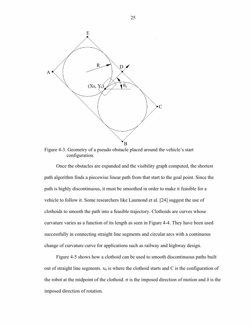
• Pseudo obstacles are placed at the start and goal points in order to ensure that the path generated obeys the initial and final orientations of the vehicle. This is as shown in Figure 4-3. ABCDE forms the pseudo obstacle that forces the path to go through a pseudo start point D.
• Since the shortest path always goes through convex vertices of the obstacle polygons and concave vertices of the boundary, these vertices are tagged as legal, while all other vertices are tagged as illegal vertices. This reduces the search time
24
of the algorithm by not considering illegal vertices in the search for the shortest path.
work space configuration space
shortest path visibility graph
Figure 4-2. Graphic representation of program flow.
Obstacle Expansion
As stated earlier, a popular simplification of the path planning problem is to grow
the obstacles in order to reduce the vehicle down to a point. The obstacle expansion stage
of the algorithm is responsible for this transformation of the vehicle to a point in the
discretized map. This stage of the algorithm is important from the point of view of the
correctness of the output path. The obstacle expansion stage must not only allow for the
computation of a collision free path, but must also guarantee that the path is an image of
an admissible trajectory. The method used to expand the obstacles and shrink the
boundary is described here in detail. It is also proved to guarantee paths that are images
of admissible trajectories.
25
E
R DA
θs (Xs, Ys)
C
Figure 4-3. Geometry of a pseudo obstacle placed around the vehicle’s start
configuration.
B
Once the obstacles are expanded and the visibility graph computed, the shortest
path algorithm finds a piecewise linear path from that start to the goal point. Since the
path is highly discontinuous, it must be smoothed in order to make it feasible for a
vehicle to follow it. Some researchers like Laumond et al. [24] suggest the use of
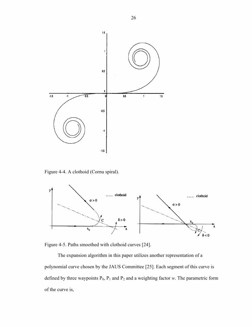
clothoids to smooth the path into a feasible trajectory. Clothoids are curves whose
curvature varies as a function of its length as seen in Figure 4-4. They have been used
successfully in connecting straight line segments and circular arcs with a continuous
change of curvature curve for applications such as railway and highway design.
Figure 4-5 shows how a clothoid can be used to smooth discontinuous paths built
out of straight line segments. x0 is where the clothoid starts and C is the configuration of
the robot at the midpoint of the clothoid. σ is the imposed direction of motion and δ is the
imposed direction of rotation.
26
Figure 4-4. A clothoid (Cornu spiral).
Figure 4-5. Paths smoothed with clothoid curves [24].
The expansion algorithm in this paper utilizes another representation of a
polynomial curve chosen by the JAUS Committee [25]. Each segment of this curve is
defined by three waypoints P0, P1 and P2 and a weighting factor w. The parametric form
of the curve is,
27
222
210
2
)1(2)1()1(2)1(
)(uwuuu
PuPwuuPuup+−+−+−+−
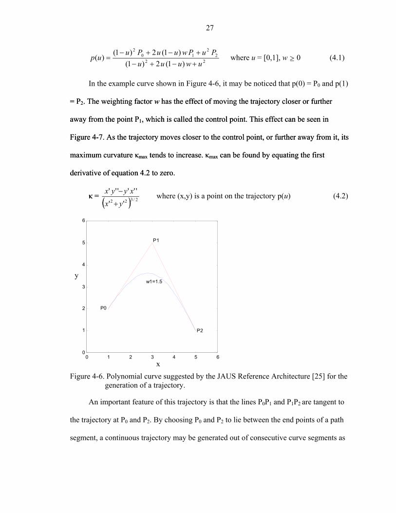
= where u = [0,1], w ≥ 0 (4.1)
In the example curve shown in Figure 4-6, it may be noticed that p(0) = P0 and p(1)
= P2. The weighting factor w has the effect of moving the trajectory closer or further
away from the point P1, which is called the control point. This effect can be seen in
Figure 4-7. As the trajectory moves closer to the control point, or further away from it, its
maximum curvature κmax tends to increase. κmax can be found by equating the first
derivative of equation 4.2 to zero.
κ = κ = ( )( ) 2/322 ''
''''''yx
xyyx+
− where (x,y) is a point on the trajectory p(u) (4.2)
0 1 2 3 4 5 60
1
2
3
4
5
6
w1=1.5
P0
P1
P2
y
x Figure 4-6. Polynomial curve suggested by the JAUS Reference Architecture [25] for the
generation of a trajectory.
An important feature of this trajectory is that the lines P0P1 and P1P2 are tangent to
the trajectory at P0 and P2. By choosing P0 and P2 to lie between the end points of a path
segment, a continuous trajectory may be generated out of consecutive curve segments as
28
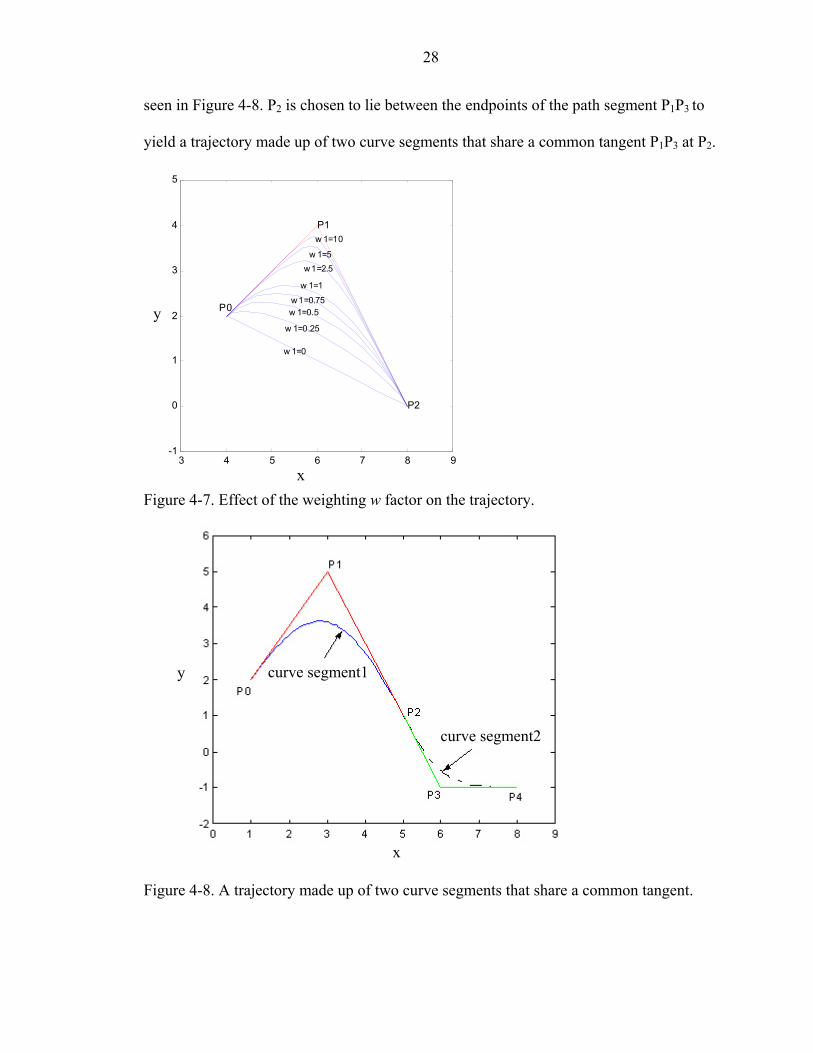
seen in Figure 4-8. P2 is chosen to lie between the endpoints of the path segment P1P3 to
yield a trajectory made up of two curve segments that share a common tangent P1P3 at P2.
3 4 5 6 7 8 9-1
0
1
2
3
4
5
w 1=10
w 1=5w1=2.5
w 1=1w1=0.75w 1=0.5
w 1=0.25
w 1=0
P0
P1
P2
y
x Figure 4-7. Effect of the weighting w factor on the trajectory.
curve segment1 y
curve segment2
x
Figure 4-8. A trajectory made up of two curve segments that share a common tangent.
29
This feature was used to develop an effective expansion method that guarantees an
admissible trajectory for any shortest path in the map. Since the waypoints along the
shortest path coincide with only convex vertices of the obstacles, the expansion of convex
vertices must ensure that any trajectory going through them lies in free space and has a
maximum curvature less than 1/R. The concave vertices must be expanded only to
maintain a sufficient offset along the walls of the obstacles in order to ensure collision
free paths in the concave regions of the obstacles. The following sections describe the
geometry behind the expansion method for convex and concave vertices.
Expansion of Convex Obstacle Vertices
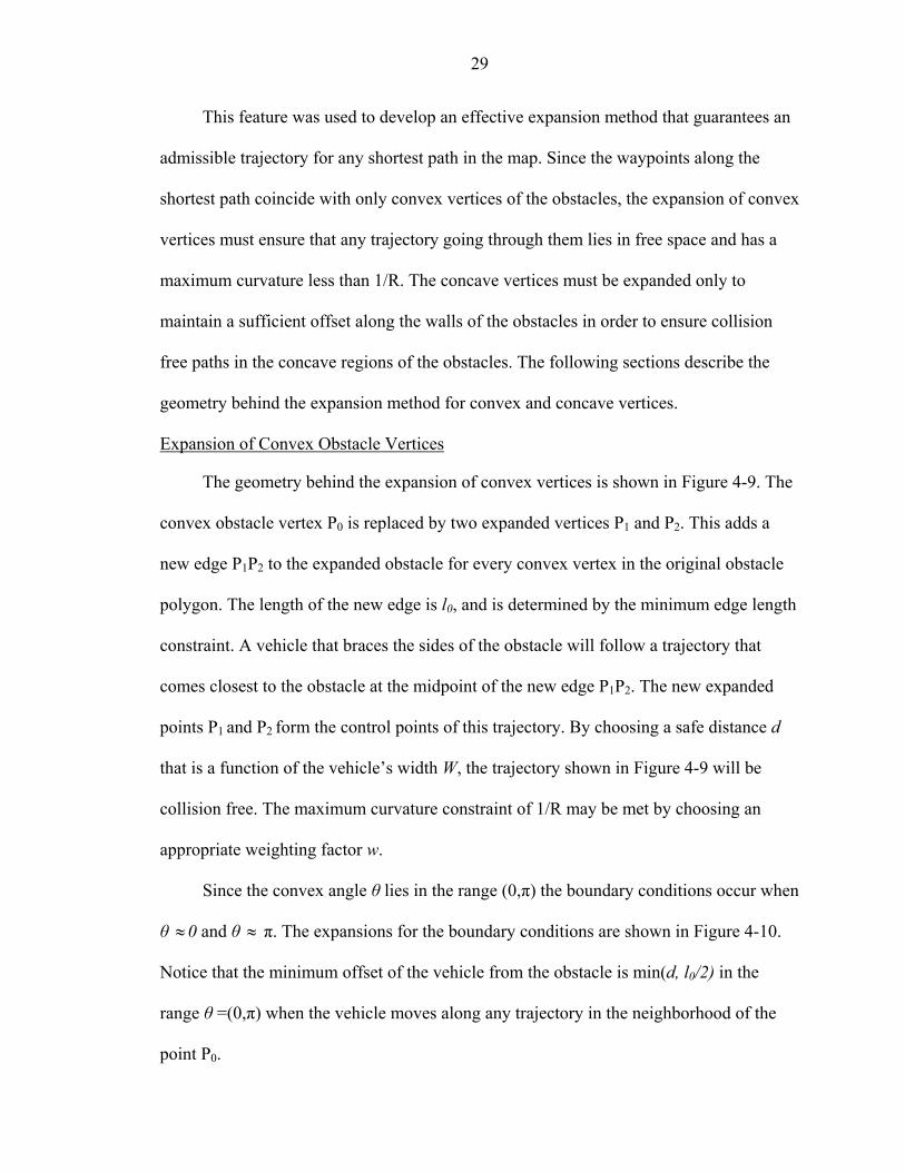
The geometry behind the expansion of convex vertices is shown in Figure 4-9. The
convex obstacle vertex P0 is replaced by two expanded vertices P1 and P2. This adds a
new edge P1P2 to the expanded obstacle for every convex vertex in the original obstacle
polygon. The length of the new edge is l0, and is determined by the minimum edge length
constraint. A vehicle that braces the sides of the obstacle will follow a trajectory that
comes closest to the obstacle at the midpoint of the new edge P1P2. The new expanded
points P1 and P2 form the control points of this trajectory. By choosing a safe distance d
that is a function of the vehicle’s width W, the trajectory shown in Figure 4-9 will be
collision free. The maximum curvature constraint of 1/R may be met by choosing an
appropriate weighting factor w.
Since the convex angle θ lies in the range (0,π) the boundary conditions occur when
θ 0 and θ ≈ π. The expansions for the boundary conditions are shown in Figure 4-10.
Notice that the minimum offset of the vehicle from the obstacle is min(d, l
≈
0/2) in the
range θ =(0,π) when the vehicle moves along any trajectory in the neighborhood of the
point P0.
30
l0 / 2 l0 / 2
P2 P1
d P0
θ/2 θ/2
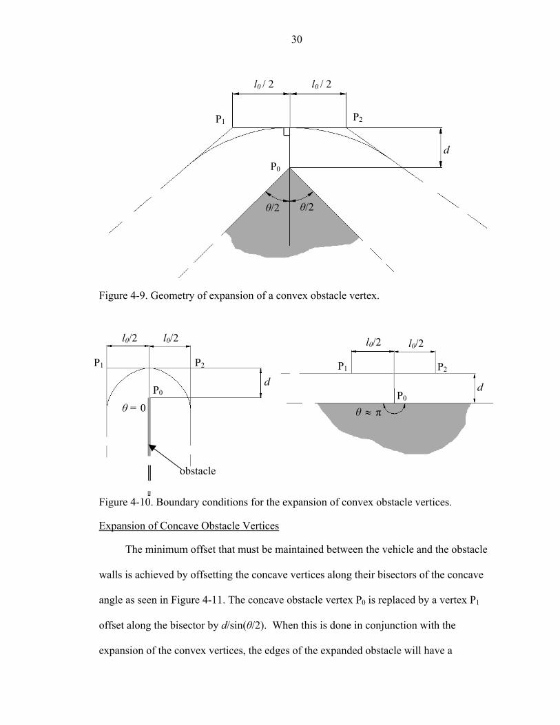
Figure 4-9. Geometry of expansion of a convex obstacle vertex.
l0/2 l0/2 l0/2 l0/2
P1 P2 P1 P2 d d P0 P0
θ = 0 θ ≈ π
obstacle
Figure 4-10. Boundary conditions for the expansion of convex obstacle vertices.
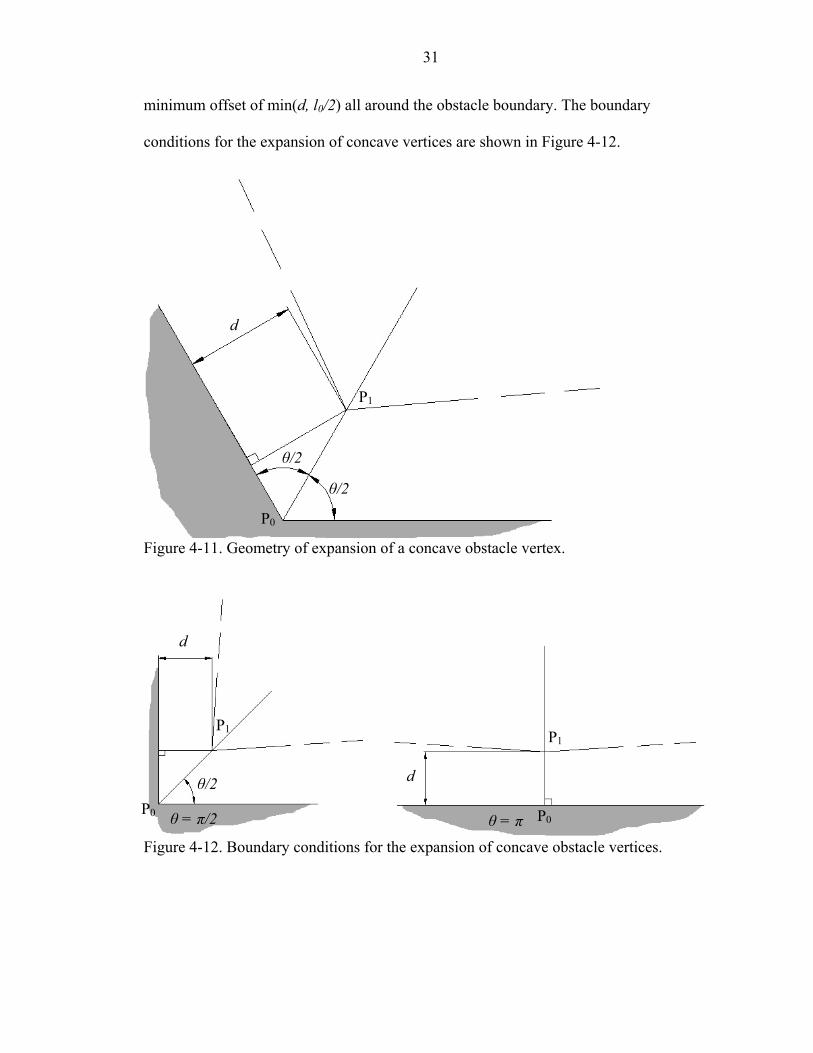
Expansion of Concave Obstacle Vertices
The minimum offset that must be maintained between the vehicle and the obstacle
walls is achieved by offsetting the concave vertices along their bisectors of the concave
angle as seen in Figure 4-11. The concave obstacle vertex P0 is replaced by a vertex P1
offset along the bisector by d/sin(θ/2). When this is done in conjunction with the
expansion of the convex vertices, the edges of the expanded obstacle will have a
31
minimum offset of min(d, l0/2) all around the obstacle boundary. The boundary
conditions for the expansion of concave vertices are shown in Figure 4-12.
d
P1
θ/2
θ/2
P0
Figure 4-11. Geometry of expansion of a concave obstacle vertex.
d
P1 P1
d θ/2 P0 P0θ = π/2 θ = πFigure 4-12. Boundary conditions for the expansion of concave obstacle vertices.
32
Main Result: Expansion Method Guarantees Admissible Trajectories
Any shortest path in a map with expanded obstacles is an image of an admissible
trajectory.
Proof: The shortest path between any given start and goal configuration uses the
expanded convex vertices of the obstacles as waypoints. The shortest path is piecewise
linear and is guaranteed to lie in free space when the obstacles are expanded with
sufficient distances d and lo. The piecewise linear path is converted into a trajectory by
using the second degree polynomial curve described by equation 4.1 to smooth the
corners of the path. This is done by choosing the vertices or waypoints of the path as
control points of the smoothing curve segments, and endpoints of the smoothing curves
along the length of the path segments adjacent to the path vertices (Figure 4-8.). In order
to prove that any shortest path among expanded obstacles is an image of an admissible
trajectory, it is sufficient to prove that the curve segments used to smooth the path lie in
free space and have a maximum curvature of 1/R.
The curve segment shown in Figure 4-6 can be made symmetric about the control
point by choosing segments P0P1 and P1P2 to be of equal length, say l0/2. Assuming that
each path segment has a length of at least l0, the path will be made up of a sequence of
segments of the type,
CaSbCa , where π < a π/2, b 0. ≤ ≥
C represents segments of the polynomial curve used for smoothing and S represents a
straight line segment of the path. a represents the acute angle at the control point and b,
the length of the straight line segments.
Notice that as the angle of a convex obstacle vertex ranges from (0, π), the inner
angle at each of the two expanded vertices (P1 and P2 in Figure 4-10) has the range (π/2,
33
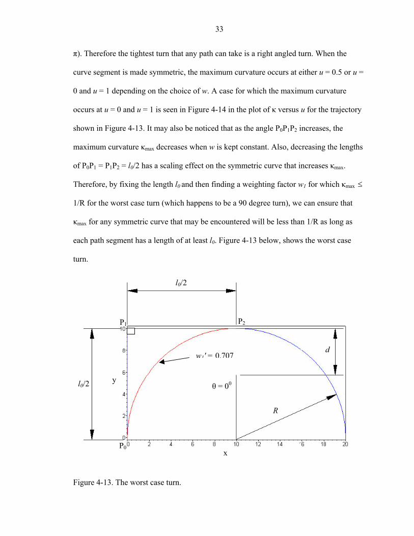
π). Therefore the tightest turn that any path can take is a right angled turn. When the
curve segment is made symmetric, the maximum curvature occurs at either u = 0.5 or u =
0 and u = 1 depending on the choice of w. A case for which the maximum curvature
occurs at u = 0 and u = 1 is seen in Figure 4-14 in the plot of κ versus u for the trajectory
shown in Figure 4-13. It may also be noticed that as the angle P0P1P2 increases, the
maximum curvature κmax decreases when w is kept constant. Also, decreasing the lengths
of P0P1 = P1P2 = l0/2 has a scaling effect on the symmetric curve that increases κmax.
Therefore, by fixing the length l0 and then finding a weighting factor w1 for which κmax ≤
1/R for the worst case turn (which happens to be a 90 degree turn), we can ensure that
κmax for any symmetric curve that may be encountered will be less than 1/R as long as
each path segment has a length of at least l0. Figure 4-13 below, shows the worst case
turn.
l0/2
P2 P1
d w1' = 0.707
y l0/2 θ = 00
R
P0 x
Figure 4-13. The worst case turn.
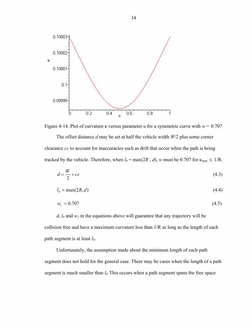
34
κ
Figure 4-14. Plot of curvature κ versus parameter u for a symmetric curve with w = 0.707
The offset distance d may be set at half the vehicle width W/2 plus some corner
clearance cc to account for inaccuracies such as drift that occur when the path is being
tracked by the vehicle. Therefore, when l0 = max(2R , d), w must be 0.707 for κmax ≤ 1/R.
ccWd +=2
(4.3)
),2max(0 dRl = (4.4)
707.01 =w (4.5)
d, l0 and w1 in the equations above will guarantee that any trajectory will be
collision free and have a maximum curvature less than 1/R as long as the length of each
path segment is at least l0.
Unfortunately, the assumption made about the minimum length of each path
segment does not hold for the general case. There may be cases when the length of a path
segment is much smaller than l0. This occurs when a path segment spans the free space
35
between two obstacles as against bracing an obstacle edge. The case for which a path
length is less than l0 is treated as a special case as follows.
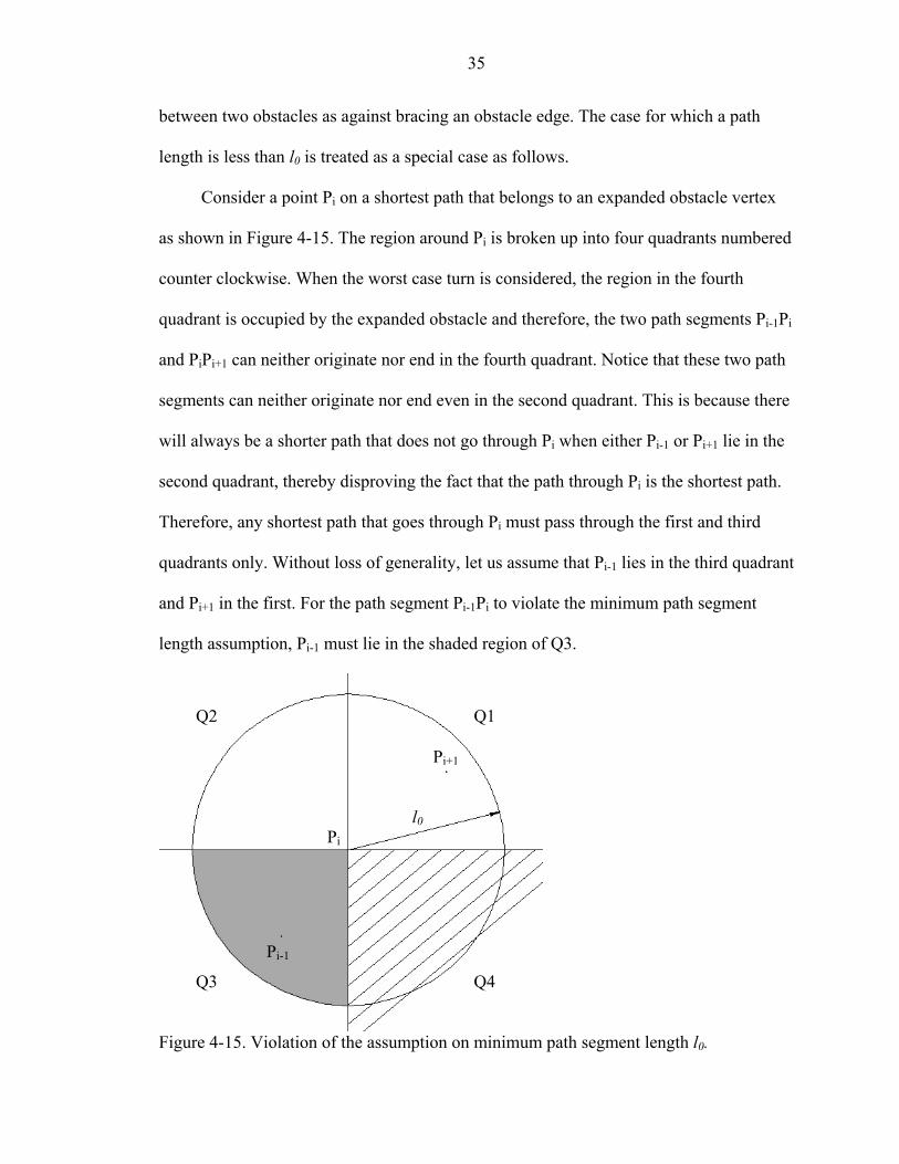
Consider a point Pi on a shortest path that belongs to an expanded obstacle vertex
as shown in Figure 4-15. The region around Pi is broken up into four quadrants numbered
counter clockwise. When the worst case turn is considered, the region in the fourth
quadrant is occupied by the expanded obstacle and therefore, the two path segments Pi-1Pi
and PiPi+1 can neither originate nor end in the fourth quadrant. Notice that these two path
segments can neither originate nor end even in the second quadrant. This is because there
will always be a shorter path that does not go through Pi when either Pi-1 or Pi+1 lie in the
second quadrant, thereby disproving the fact that the path through Pi is the shortest path.
Therefore, any shortest path that goes through Pi must pass through the first and third
quadrants only. Without loss of generality, let us assume that Pi-1 lies in the third quadrant
and Pi+1 in the first. For the path segment Pi-1Pi to violate the minimum path segment
length assumption, Pi-1 must lie in the shaded region of Q3.
Q2 Q1
Pi+1
l0 Pi
Pi-1
Q3 Q4
Figure 4-15. Violation of the assumption on minimum path segment length l0.
36
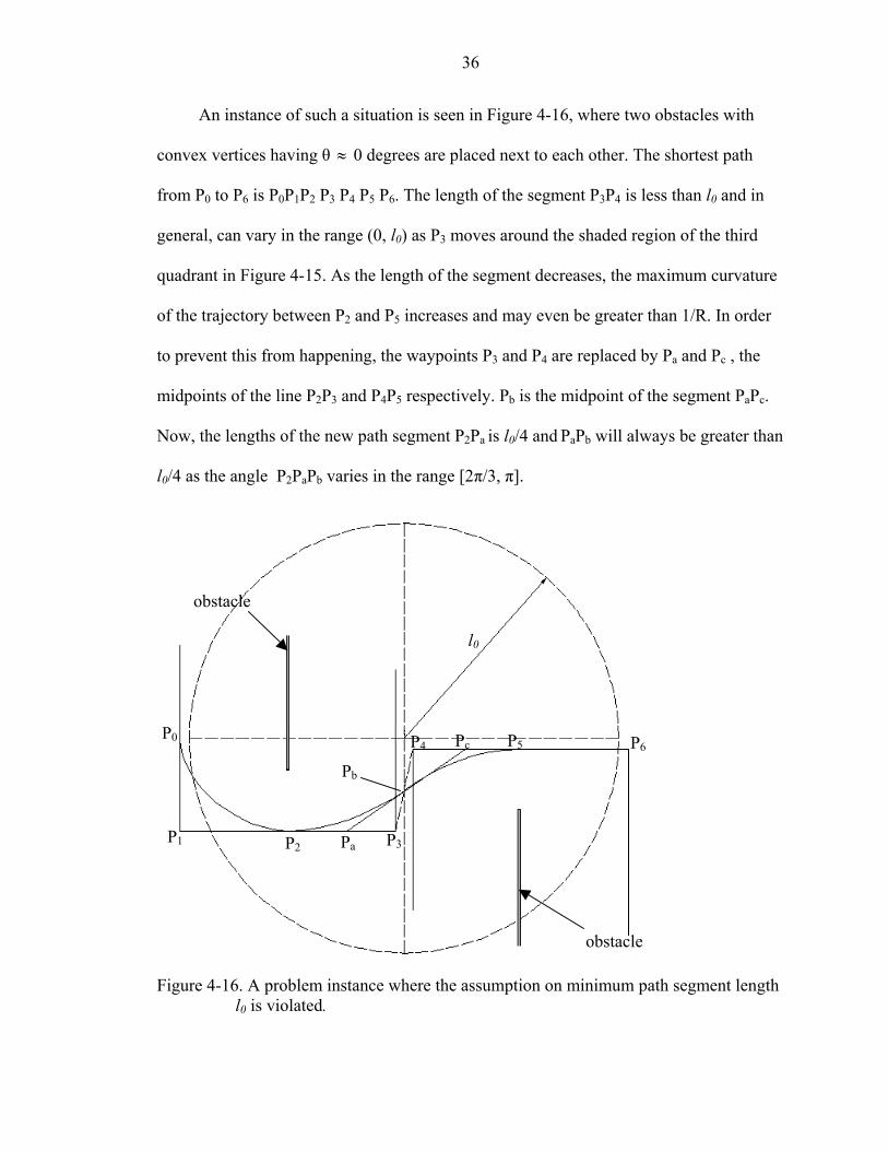
An instance of such a situation is seen in Figure 4-16, where two obstacles with
convex vertices having θ 0 degrees are placed next to each other. The shortest path
from P
≈
0 to P6 is P0P1P2 P3 P4 P5 P6. The length of the segment P3P4 is less than l0 and in
general, can vary in the range (0, l0) as P3 moves around the shaded region of the third
quadrant in Figure 4-15. As the length of the segment decreases, the maximum curvature
of the trajectory between P2 and P5 increases and may even be greater than 1/R. In order
to prevent this from happening, the waypoints P3 and P4 are replaced by Pa and Pc , the
midpoints of the line P2P3 and P4P5 respectively. Pb is the midpoint of the segment PaPc.
Now, the lengths of the new path segment P2Pa is l0/4 and PaPb will always be greater than
l0/4 as the angle P2PaPb varies in the range [2π/3, π].
P3
P4
P2
P5
Pa
l0
Pb
Pc
obstacle
P0 P6
P1
obstacle
Figure 4-16. A problem instance where the assumption on minimum path segment length l0 is violated.
37
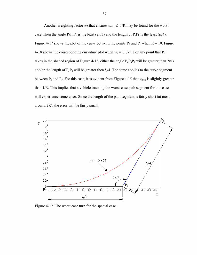
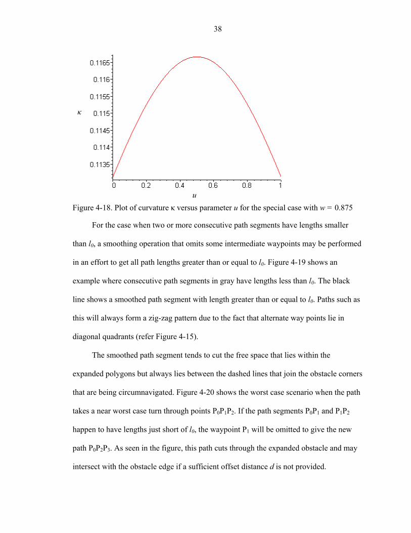
Another weighting factor w2 that ensures κmax ≤ 1/R may be found for the worst
case when the angle P2PaPb is the least (2π/3) and the length of PaPb is the least (l0/4).
Figure 4-17 shows the plot of the curve between the points P2 and Pb when R = 10. Figure
4-18 shows the corresponding curvature plot when w2 = 0.875. For any point that P3
takes in the shaded region of Figure 4-15, either the angle P2PaPb will be greater than 2π/3
and/or the length of P3Pa will be greater then l0/4. The same applies to the curve segment
between Pb and P5. For this case, it is evident from Figure 4-15 that κmax is slightly greater
than 1/R. This implies that a vehicle tracking the worst-case path segment for this case
will experience some error. Since the length of the path segment is fairly short (at most
around 2R), the error will be fairly small.
Pb y
w2 = 0.875 l0/4
2π/3
Pa P2
x l0/4
Figure 4-17. The worst case turn for the special case.
38
κ
u Figure 4-18. Plot of curvature κ versus parameter u for the special case with w = 0.875
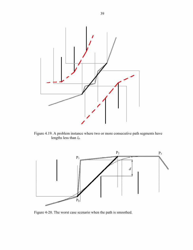
For the case when two or more consecutive path segments have lengths smaller
than l0, a smoothing operation that omits some intermediate waypoints may be performed
in an effort to get all path lengths greater than or equal to l0. Figure 4-19 shows an
example where consecutive path segments in gray have lengths less than l0. The black
line shows a smoothed path segment with length greater than or equal to l0. Paths such as
this will always form a zig-zag pattern due to the fact that alternate way points lie in
diagonal quadrants (refer Figure 4-15).
The smoothed path segment tends to cut the free space that lies within the
expanded polygons but always lies between the dashed lines that join the obstacle corners
that are being circumnavigated. Figure 4-20 shows the worst case scenario when the path
takes a near worst case turn through points P0P1P2. If the path segments P0P1 and P1P2
happen to have lengths just short of l0, the waypoint P1 will be omitted to give the new
path P0P2P3. As seen in the figure, this path cuts through the expanded obstacle and may
intersect with the obstacle edge if a sufficient offset distance d is not provided.
39
Figure 4.19. A problem instance where two or more consecutive path segments have
lengths less than l0.
P2 P3P1
d
P0
Figure 4-20. The worst case scenario when the path is smoothed.
40
To accommodate for this case, the variable d in equation 4.3 must be further
relaxed and the final form of all the expansion variables are listed below.
ccWRd ++=2
(4.6)
),2max(0 dRl = (4.7)
707.01 =w , w2 = 0.875 (4.8)
The use of variables d, l0, w1 and w2 in the equations above, will ensure that any
shortest path in the configuration space created by the proposed expansion method is an
image of an admissible trajectory.
The shrinking of the boundary polygon is the exact opposite of the expansion of the
obstacle polygons. Concave boundary vertices are shrunk in a manner similar to the
convex vertex expansion of obstacles, and vice versa. This is easily done by running the
obstacle expansion algorithm on the boundary polygon after its orientation has been
switched from counter clockwise to clockwise temporarily. Once the boundary polygon is
shrunk, the orientation is reversed again to obey the CCW convention.
After the expansion, expanded convex vertices that lie in the interior of obstacles
(due to polygon intersections) or to the exterior of the boundary are also tagged as illegal
vertices.
Visibility Graph
Once the obstacles are expanded to guarantee that the shortest path is an image of
an admissible trajectory, the map must be decomposed into a graph data structure denoted
by G = (V, E), where V is a set of nodes and E is a set of edges connecting the nodes in V.
G is a bi-directional graph whose nodes represent the legal vertices in the map and whose
edges carry weights that are equal to the line of sight distance between the legal vertices.
41
The graph is chosen to be represented as by an adjacency matrix M, where M[i][j] gives
the distance between the vertex Pi and vertex Pj if both are legal vertices. M is symmetric
about its diagonal and has the size n2, where n is the number of legal vertices in the map.
A natural brute force method to fill the adjacency matrix is to compute the visibility of
every vertex Pi, i = 1..n with respect to every other vertex Pj, j = 1..n. In order to do this,
the line segment PiPj must be checked for intersection between every obstacle edge in the
map. If no obstacle edge intersects the edge PiPj , the vertex Pi is visible to vertex Pj and
the distance between them is entered into M[i,j] and M[j,i]. This turns out to be an O(n3)
algorithm.
The computation of the visibility graph therefore, turns out to be the bottleneck of
the shortest path algorithm. By improving the efficiency of this stage of the algorithm, the
overall algorithm speed will be greatly enhanced. de Berg et al. [26] have applied the
popular sweep line algorithm in computational geometry to the visibility graph problem
and have created an algorithm that runs in O(n2logn) time, a significant improvement
over the brute force method. This algorithm has been adapted to the path planning
implementation and is briefly described below.
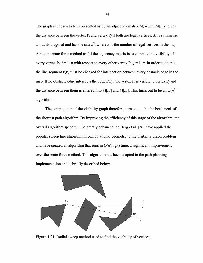
pi ρ wi-1
wi
Figure 4-21. Radial sweep method used to find the visibility of vertices.
42
The visibility graph G is first initialized such that V is the set of all legal vertices in
the graph and E = 0. For each vertex pi∈V , i=1..n create a sorted list W of legal vertices
in the map according to the clockwise angle made by the half line joining pi to each
vertex and the positive x-axis. Ties are broken by virtue of the distance from pi. Initialize
the half line ρ with the positive x-axis as seen in Figure 4-21. Find all obstacle edges that
properly intersect ρ and store them in a balanced search tree τ in the order in which they
intersect ρ. For each vertex wj ∈ W, j = 1..n the following operations are performed to
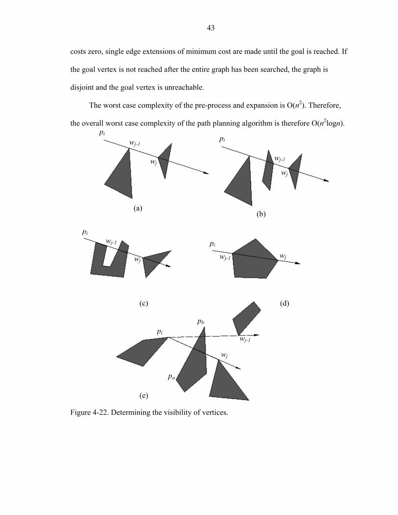
find if wj is visible to pi.
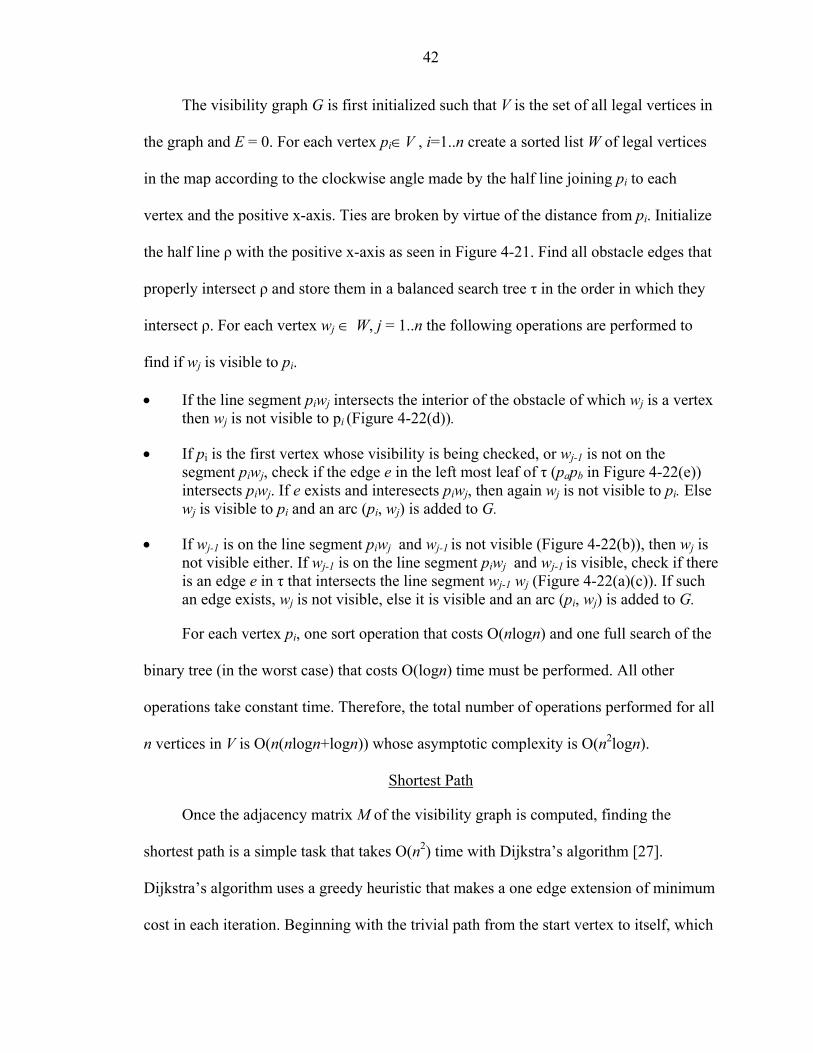
• If the line segment piwj intersects the interior of the obstacle of which wj is a vertex then wj is not visible to pi (Figure 4-22(d)).
• If pi is the first vertex whose visibility is being checked, or wj-1 is not on the segment piwj, check if the edge e in the left most leaf of τ (papb in Figure 4-22(e)) intersects piwj. If e exists and interesects piwj, then again wj is not visible to pi. Else wj is visible to pi and an arc (pi, wj) is added to G.
• If wj-1 is on the line segment piwj and wj-1 is not visible (Figure 4-22(b)), then wj is not visible either. If wj-1 is on the line segment piwj and wj-1 is visible, check if there is an edge e in τ that intersects the line segment wj-1 wj (Figure 4-22(a)(c)). If such an edge exists, wj is not visible, else it is visible and an arc (pi, wj) is added to G.
For each vertex pi, one sort operation that costs O(nlogn) and one full search of the
binary tree (in the worst case) that costs O(logn) time must be performed. All other
operations take constant time. Therefore, the total number of operations performed for all
n vertices in V is O(n(nlogn+logn)) whose asymptotic complexity is O(n2logn).
Shortest Path
Once the adjacency matrix M of the visibility graph is computed, finding the
shortest path is a simple task that takes O(n2) time with Dijkstra’s algorithm [27].
Dijkstra’s algorithm uses a greedy heuristic that makes a one edge extension of minimum
cost in each iteration. Beginning with the trivial path from the start vertex to itself, which
43
costs zero, single edge extensions of minimum cost are made until the goal is reached. If
the goal vertex is not reached after the entire graph has been searched, the graph is
disjoint and the goal vertex is unreachable.
The worst case complexity of the pre-process and expansion is O(n2). Therefore,
the overall worst case complexity of the path planning algorithm is therefore O(n2logn).
pi pi wj-1
wj-1 wj
wj
(a) (b)
pi wj-1 pi
wj wj-1 wj
(c) (d)
pb
pi wj-1
wj
pa
(e)
Figure 4-22. Determining the visibility of vertices.
CHAPTER 5 PATH PLANNING WITH A RADIATION CONSTRAINT
This section describes one possible way of planning paths in a constrained
environment using the path planner. The algorithm described here utilizes the path
planner to lower the dose received by a mobile robot moving in a radiation field. We look
at the problem in the plane of the robot and for the sake of simplicity, assume that the
radiation sources are point sources that are placed in the same plane. The algorithm was
initially designed and implemented without considering attenuation from obstacles. An
extension that allows the algorithm to consider attenuation was later designed and is
presented in appendix A.
Radiation Basics
Of the many different forms of radiation emanated from radioactive materials,
gamma rays are by far the most harmful from the point of view of robotic equipment.
Exposure to gamma radiation can be minimized by following a basic ALARA principle
[28] that states, by reducing the amount of time spent near a source of radiation,
increasing the distance between the source and the robot, and by using shielding material
placed between the source and the robot reduces the exposure to radiation.
The effect of radiation exposure may be measured using the units rad (radiation
absorbed dose) and rem (Roentgen Equivalent Man). Rad is used to measure the quantity
of absorbed dose in terms of the amount of energy actually absorbed by a material, while
rem is used to derive an equivalent dose based on the type of radiation being emanated.
Since different types of radiation have different effects, the absorbed dose in rad was
44
45
multiplied by a quality factor Q, unique to the incident radiation, to get the equivalent
dose in rem. In recent years, these units have been replaced by two new SI units – gray
(Gy) and sievert (Sv).
One gray represents the energy absorption of 1 joule per kilogram of absorbing
material. That is,
1 Gy = 1 J Kg-1 (5.1)
The unit Gray replaced rad as the choice of absorbed dose and sievert replaced rem
as the new choice for equivalent dose. The equivalent dose in sievert for a given type of
radiation was defined as
H = D x wh (5.2)
H is the equivalent dose in sievert, D is the absorbed dose in gray and wh is the
radiation weighting factor that is dependant on the type of incident radiation.
The amount of radiation absorbed by a material per unit time is given by the
equivalent dose rate or simply dose rate. Dose rate is usually measured in sieverts per
unit time, that is Svh-1 or more usually mSvh-1. The cumulative dose is the integral of dose
rate over time and represents the total amount of radiation absorbed.
The intensity of the absorbed radiation depends on the absorption of radiation by
the air and the shape and size of the source relative to the distance from which it is
viewed. Gamma rays are not scattered by air and therefore, their intensity is determined
as a function of the distance from the source. Most numerical computations and
simulations that deal with gamma radiation consider the shape of the source to be a point,
line or an extended source. Point sources are used when the radioactive material is
believed to be emitting equal quantities of radiation in all directions. Line sources
46
represent pipe like structures while extended sources are used to represent large areas like
walls and floors.
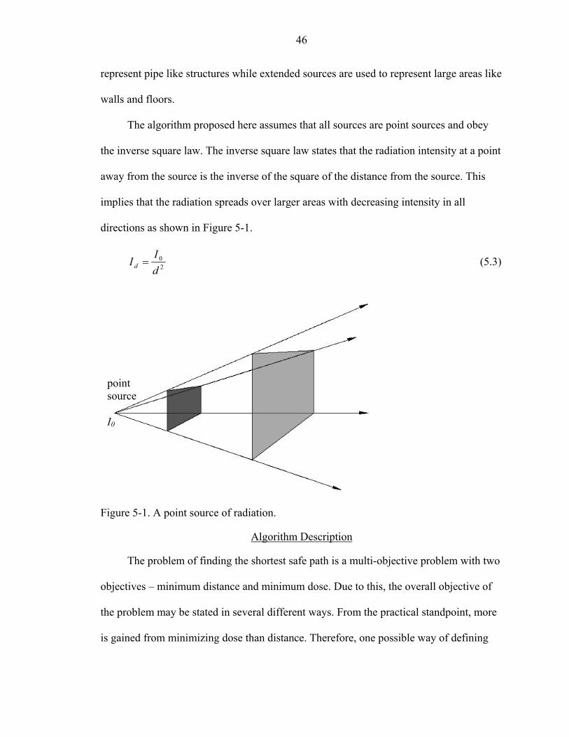
The algorithm proposed here assumes that all sources are point sources and obey
the inverse square law. The inverse square law states that the radiation intensity at a point
away from the source is the inverse of the square of the distance from the source. This
implies that the radiation spreads over larger areas with decreasing intensity in all
directions as shown in Figure 5-1.
20
dI
I d = (5.3)
point source I0
Figure 5-1. A point source of radiation.
Algorithm Description
The problem of finding the shortest safe path is a multi-objective problem with two
objectives – minimum distance and minimum dose. Due to this, the overall objective of
the problem may be stated in several different ways. From the practical standpoint, more
is gained from minimizing dose than distance. Therefore, one possible way of defining
47
the global optimal path Popt is, a path with the least dose absorption. That is, no other path
in the map has a cumulative dose absorption less than the path Popt.
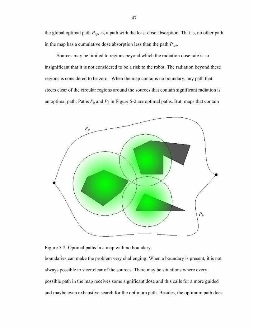
Sources may be limited to regions beyond which the radiation dose rate is so
insignificant that it is not considered to be a risk to the robot. The radiation beyond these
regions is considered to be zero. When the map contains no boundary, any path that
steers clear of the circular regions around the sources that contain significant radiation is
an optimal path. Paths Pa and Pb in Figure 5-2 are optimal paths. But, maps that contain
Pa
Pb
Figure 5-2. Optimal paths in a map with no boundary.
boundaries can make the problem very challenging. When a boundary is present, it is not
always possible to steer clear of the sources. There may be situations where every
possible path in the map receives some significant dose and this calls for a more guided
and maybe even exhaustive search for the optimum path. Besides, the optimum path does

48
not necessarily have to pass through the vertices of the discretized map. This implies that
a graph type algorithm can only achieve a near optimal result. From this point of view, it
may be better to approach this problem using some other approach like the potential field
method or a randomized heuristic. But, due to the complex nature of radiation fields,
these approaches also cannot guarantee the global optimal path. They may only pro7vide
better approximations when compared to a graph search method, but at higher
computational costs.
The cumulative dose absorbed by the robot is lessened by using the path planner to
enforce the basic ALARA principle of increasing the distance of the robot from the
sources to reduce exposure. The exposure is minimized by beginning with the shortest
path and moving this path away from the radiation sources. At first, circular pseudo
obstacles of unit radius are drawn around each source. The circles are then grown
incrementally such that the intensity of the radiation at their circumference reduces by
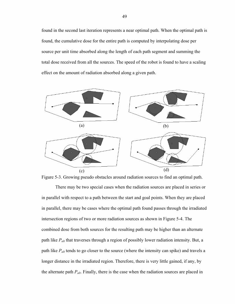
some small amount, say 1 mSvh-1 with each iteration. Figure 5-3 illustrates this concept.
The pseudo obstacles create a new type of configuration space where the dose at every
point in free space, contributed by any given source, is less than or equal to the intensity
at the circumference of the pseudo obstacles. Circles that enclose radiation sources with
relatively smaller intensities grow at slower rates than circles that enclose high intensity
sources. With each iteration, the pseudo obstacles are grown and the path planner is
executed to find if a path still exists. The iterations continue until either all the circular
pseudo obstacles have been grown to their maximum limit, (intensity of 0.1 mSvh-1 at the
circumference to prevent d from going to infinity) or when a path cannot be found. In the
former case, the shortest path happens to be the optimum path. In the latter case, the path
49
found in the second last iteration represents a near optimal path. When the optimal path is
found, the cumulative dose for the entire path is computed by interpolating dose per
source per unit time absorbed along the length of each path segment and summing the
total dose received from all the sources. The speed of the robot is found to have a scaling
effect on the amount of radiation absorbed along a given path.
(a) (b)
(d) (c) Figure 5-3. Growing pseudo obstacles around radiation sources to find an optimal path.
There may be two special cases when the radiation sources are placed in series or
in parallel with respect to a path between the start and goal points. When they are placed
in parallel, there may be cases where the optimal path found passes through the irradiated
intersection regions of two or more radiation sources as shown in Figure 5-4. The
combined dose from both sources for the resulting path may be higher than an alternate
path like Palt that traverses through a region of possibly lower radiation intensity. But, a
path like Palt tends to go closer to the source (where the intensity can spike) and travels a
longer distance in the irradiated region. Therefore, there is very little gained, if any, by
the alternate path Palt. Finally, there is the case when the radiation sources are placed in
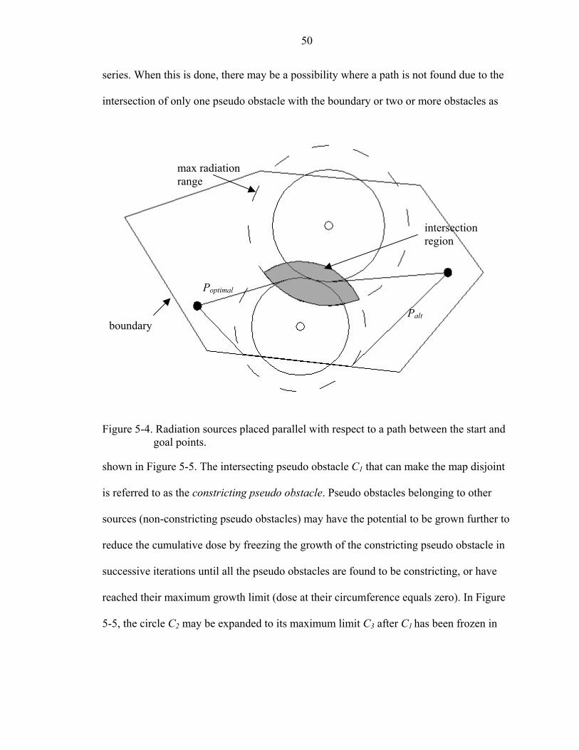
50
series. When this is done, there may be a possibility where a path is not found due to the
intersection of only one pseudo obstacle with the boundary or two or more obstacles as
max radiation range
intersection region
Poptimal
Palt boundary
Figure 5-4. Radiation sources placed parallel with respect to a path between the start and goal points.
shown in Figure 5-5. The intersecting pseudo obstacle C1 that can make the map disjoint
is referred to as the constricting pseudo obstacle. Pseudo obstacles belonging to other
sources (non-constricting pseudo obstacles) may have the potential to be grown further to
reduce the cumulative dose by freezing the growth of the constricting pseudo obstacle in
successive iterations until all the pseudo obstacles are found to be constricting, or have
reached their maximum growth limit (dose at their circumference equals zero). In Figure
5-5, the circle C2 may be expanded to its maximum limit C3 after C1 has been frozen in
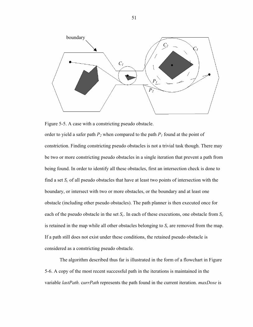
51
boundary C2 C3
C1
P1
P2
Figure 5-5. A case with a constricting pseudo obstacle.
order to yield a safer path P2 when compared to the path P1 found at the point of
constriction. Finding constricting pseudo obstacles is not a trivial task though. There may
be two or more constricting pseudo obstacles in a single iteration that prevent a path from
being found. In order to identify all these obstacles, first an intersection check is done to
find a set Sc of all pseudo obstacles that have at least two points of intersection with the
boundary, or intersect with two or more obstacles, or the boundary and at least one
obstacle (including other pseudo obstacles). The path planner is then executed once for
each of the pseudo obstacle in the set Sc. In each of these executions, one obstacle from Sc
is retained in the map while all other obstacles belonging to Sc are removed from the map.
If a path still does not exist under these conditions, the retained pseudo obstacle is
considered as a constricting pseudo obstacle.
The algorithm described thus far is illustrated in the form of a flowchart in Figure
5-6. A copy of the most recent successful path in the iterations is maintained in the
variable lastPath. currPath represents the path found in the current iteration. maxDose is
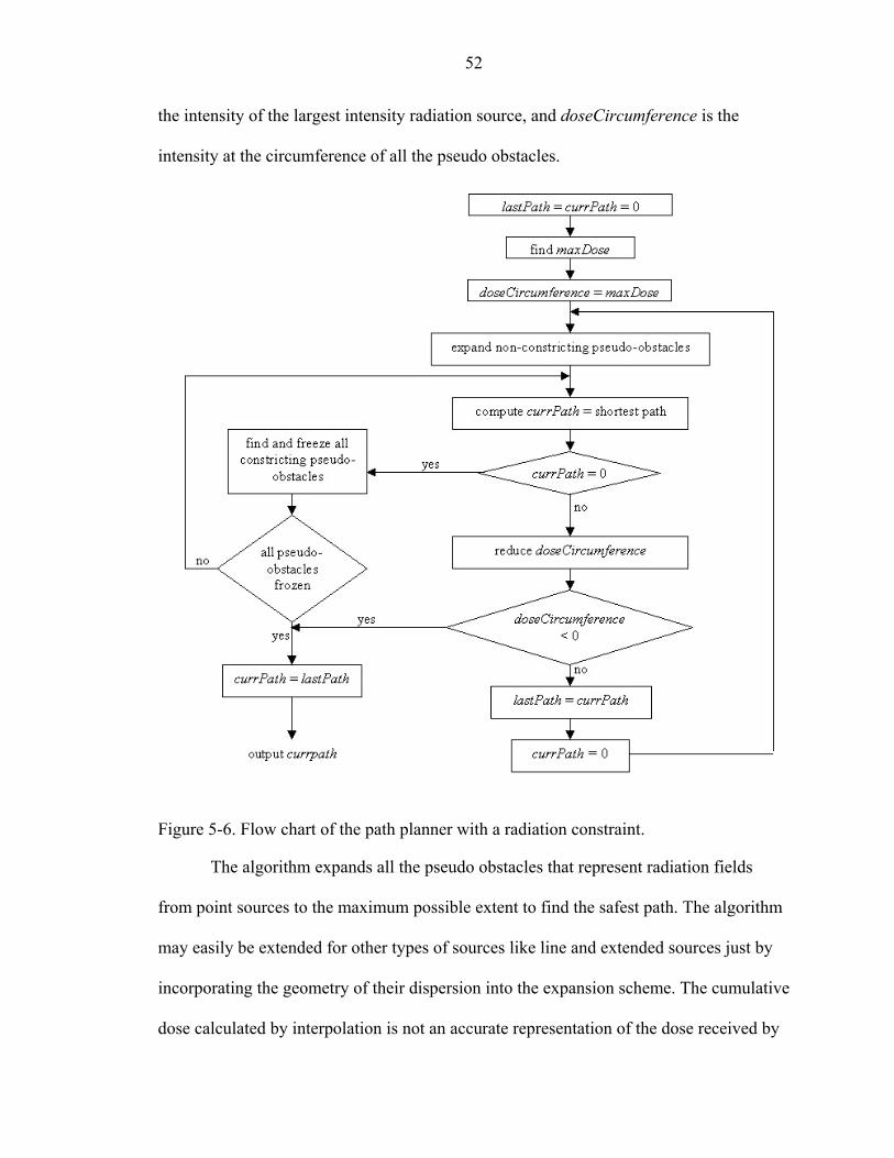
52
the intensity of the largest intensity radiation source, and doseCircumference is the
intensity at the circumference of all the pseudo obstacles.
Figure 5-6. Flow chart of the path planner with a radiation constraint.
The algorithm expands all the pseudo obstacles that represent radiation fields
from point sources to the maximum possible extent to find the safest path. The algorithm
may easily be extended for other types of sources like line and extended sources just by
incorporating the geometry of their dispersion into the expansion scheme. The cumulative
dose calculated by interpolation is not an accurate representation of the dose received by

53
the robot since a highly simplified radiation field is used to find the path. It is only used
as a relative measure to find the optimal path. The actual radiation field is more complex
due to gamma interaction processes such as pair production, Compton scattering and
buildup. Nevertheless, the resulting path is bound to be near optimal by virtue of the
basic ALARA principle.
CHAPTER 6 RESULTS AND CONCLUSION
The algorithms were implemented in C and were tested with the help of an
interactive graphical user interface developed in Java1.2. The interface linked to the C
implementation through the Java Native Interface for C. The C implementation was built
on a simple and efficient data structure that is general enough to be used for other map
based algorithms like the path sweep algorithm or path planning among moving
obstacles.
Results from sample runs of both the path planner and the path planner with
radiation constraints are shown below. Figure 6-1 shows a path being generated among a
set of expanded non-convex obstacles and a boundary. Pseudo obstacles are used to
enforce the initial and final configurations of the robot. Figure 6-2 shows the trajectory
for the path generated in Figure 6-1. Figure 6-3 is an example of the special case when
the length of a path segment is less than l0. The fourth path segment from the goal is
modified to ensure that the final trajectory is admissible. The final trajectory for this path
shown in Figure 6-4. Figure 6-5 shows the trivial case when the sets of obstacles and
boundary vertices are empty sets. The shortest path is a straight line path. Figure 6-6 and
6-7 show a case where concave boundary vertices are used to find the shortest path.
Figures 6-8 to 6-12 show example runs of the path planner with radiations sources
in the environment. Figure 6-8 shows a case when no boundary is present. Any path that
avoids the circular (approximated by octagons) regions that represent the effective reach
of the radiation is an optimum path. Figures 6-9 and 6-10 show cases where the optimum
54
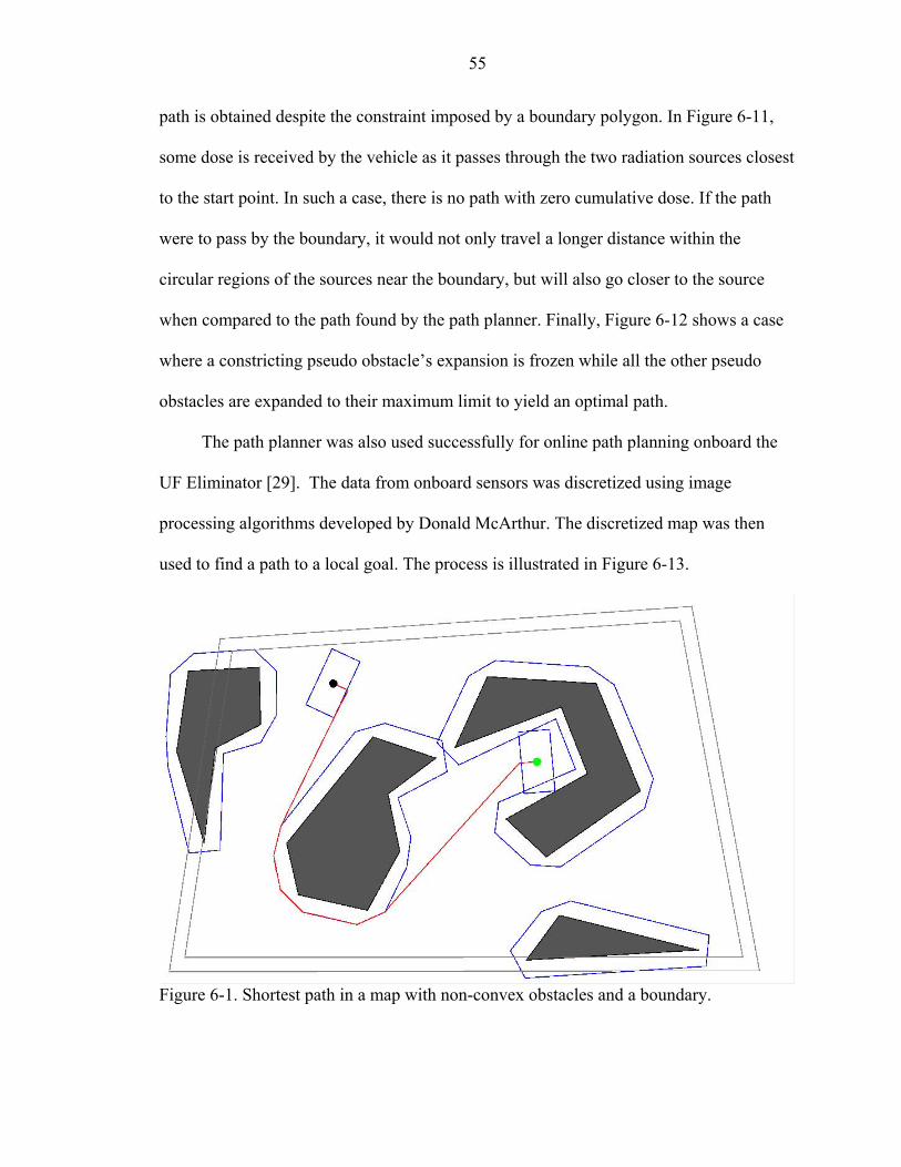
55
path is obtained despite the constraint imposed by a boundary polygon. In Figure 6-11,
some dose is received by the vehicle as it passes through the two radiation sources closest
to the start point. In such a case, there is no path with zero cumulative dose. If the path
were to pass by the boundary, it would not only travel a longer distance within the
circular regions of the sources near the boundary, but will also go closer to the source
when compared to the path found by the path planner. Finally, Figure 6-12 shows a case
where a constricting pseudo obstacle’s expansion is frozen while all the other pseudo
obstacles are expanded to their maximum limit to yield an optimal path.
The path planner was also used successfully for online path planning onboard the
UF Eliminator [29]. The data from onboard sensors was discretized using image
processing algorithms developed by Donald McArthur. The discretized map was then
used to find a path to a local goal. The process is illustrated in Figure 6-13.
Figure 6-1. Shortest path in a map with non-convex obstacles and a boundary.
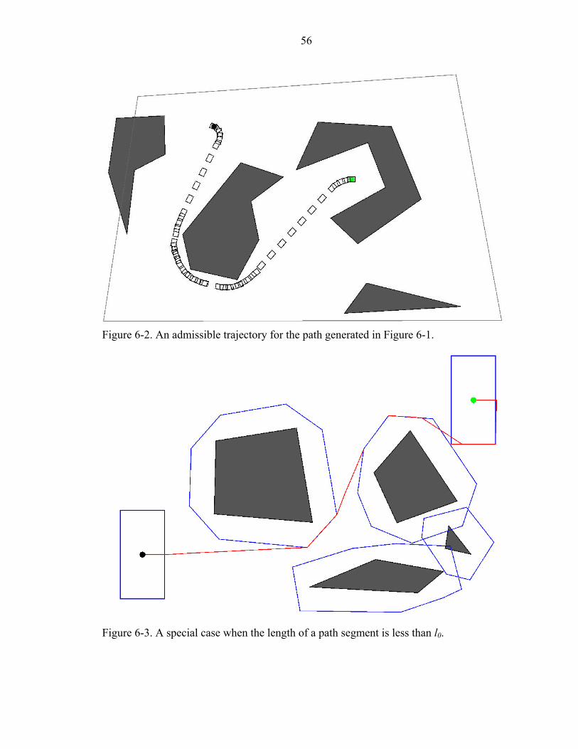
56
Figure 6-2. An admissible trajectory for the path generated in Figure 6-1.
Figure 6-3. A special case when the length of a path segment is less than l0.
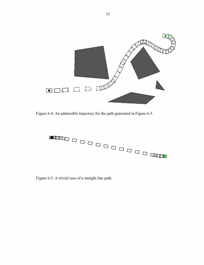
57
Figure 6-4. An admissible trajectory for the path generated in Figure 6-3.
Figure 6-5. A trivial case of a straight line path.
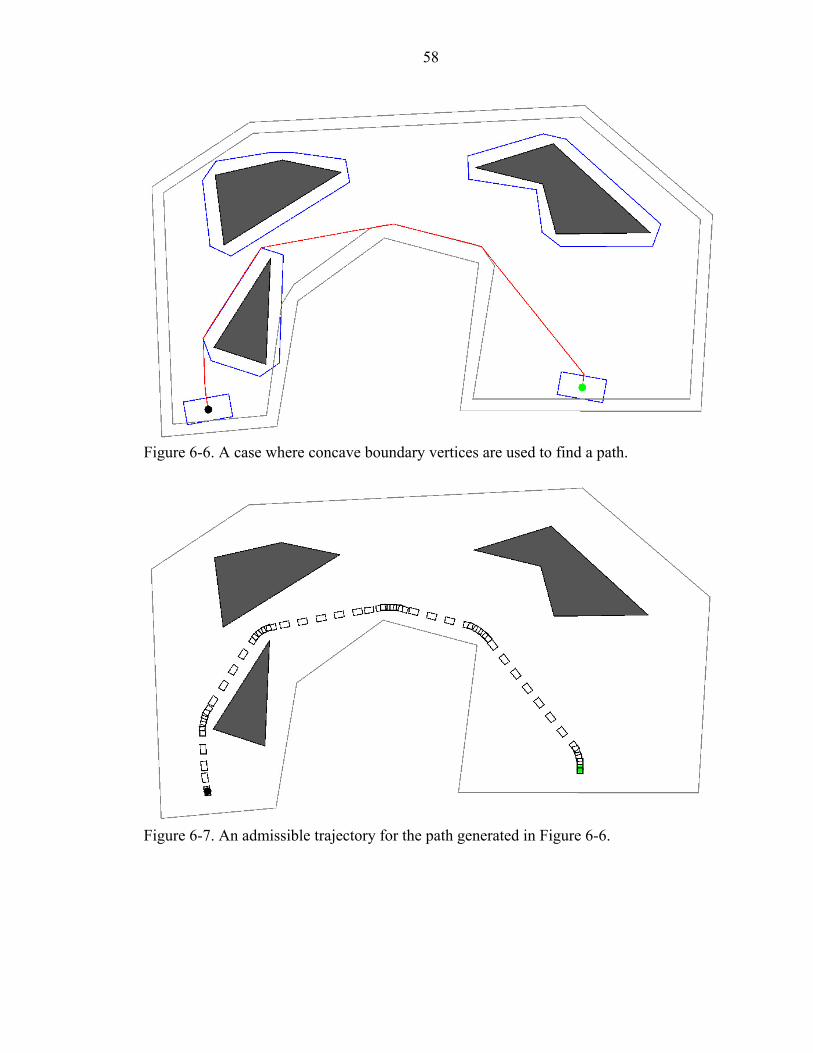
58
Figure 6-6. A case where concave boundary vertices are used to find a path.
Figure 6-7. An admissible trajectory for the path generated in Figure 6-6.
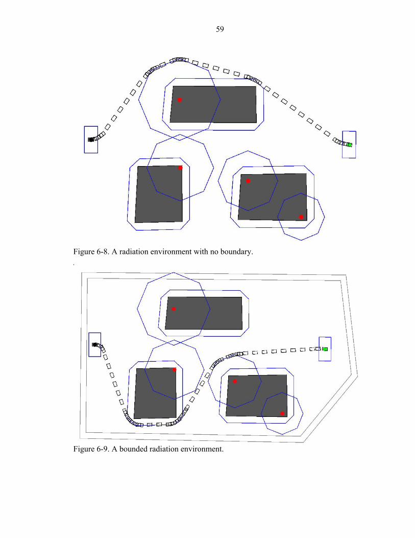
59
Figure 6-8. A radiation environment with no boundary.
Figure 6-9. A bounded radiation environment.
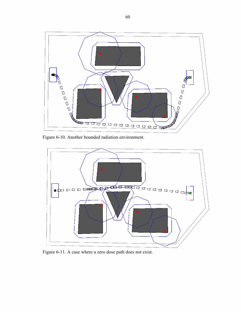
60
Figure 6-10. Another bounded radiation environment.
Figure 6-11. A case where a zero dose path does not exist.
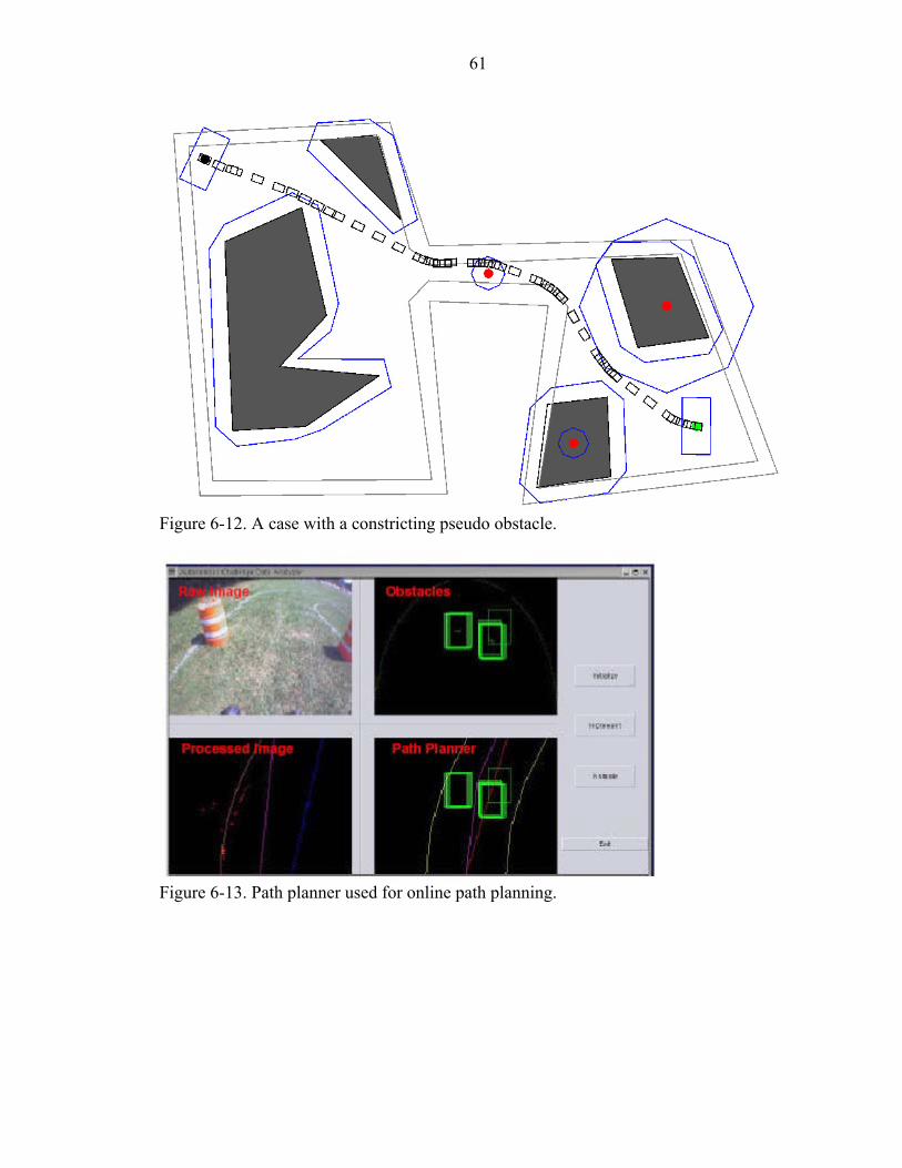
61
Figure 6-12. A case with a constricting pseudo obstacle.
Figure 6-13. Path planner used for online path planning.
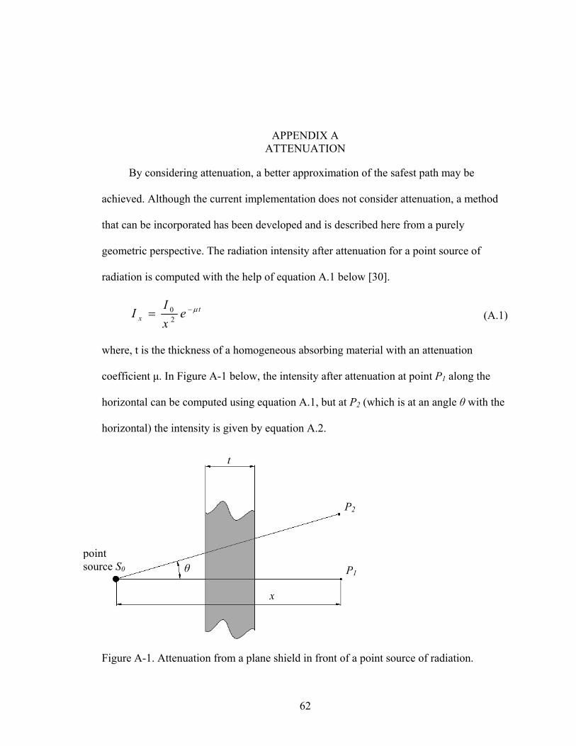
APPENDIX A ATTENUATION
By considering attenuation, a better approximation of the safest path may be
achieved. Although the current implementation does not consider attenuation, a method
that can be incorporated has been developed and is described here from a purely
geometric perspective. The radiation intensity after attenuation for a point source of
radiation is computed with the help of equation A.1 below [30].
tx e
xII µ−= 2
0 (A.1)
where, t is the thickness of a homogeneous absorbing material with an attenuation
coefficient µ. In Figure A-1 below, the intensity after attenuation at point P1 along the
horizontal can be computed using equation A.1, but at P2 (which is at an angle θ with the
horizontal) the intensity is given by equation A.2.
t
P2
point source S0 θ P1
x
Figure A-1. Attenuation from a plane shield in front of a point source of radiation.
62
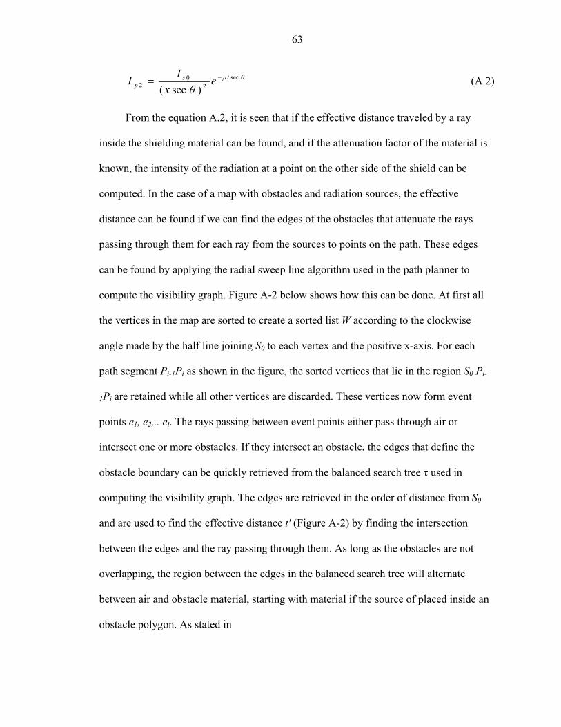
63
θµ
θsec
20
2 )sec(ts
p ex
II −= (A.2)
From the equation A.2, it is seen that if the effective distance traveled by a ray
inside the shielding material can be found, and if the attenuation factor of the material is
known, the intensity of the radiation at a point on the other side of the shield can be
computed. In the case of a map with obstacles and radiation sources, the effective
distance can be found if we can find the edges of the obstacles that attenuate the rays
passing through them for each ray from the sources to points on the path. These edges
can be found by applying the radial sweep line algorithm used in the path planner to
compute the visibility graph. Figure A-2 below shows how this can be done. At first all
the vertices in the map are sorted to create a sorted list W according to the clockwise
angle made by the half line joining S0 to each vertex and the positive x-axis. For each
path segment Pi-1Pi as shown in the figure, the sorted vertices that lie in the region S0 Pi-
1Pi are retained while all other vertices are discarded. These vertices now form event
points e1, e2,.. ei. The rays passing between event points either pass through air or
intersect one or more obstacles. If they intersect an obstacle, the edges that define the
obstacle boundary can be quickly retrieved from the balanced search tree τ used in
computing the visibility graph. The edges are retrieved in the order of distance from S0
and are used to find the effective distance t' (Figure A-2) by finding the intersection
between the edges and the ray passing through them. As long as the obstacles are not
overlapping, the region between the edges in the balanced search tree will alternate
between air and obstacle material, starting with material if the source of placed inside an
obstacle polygon. As stated in
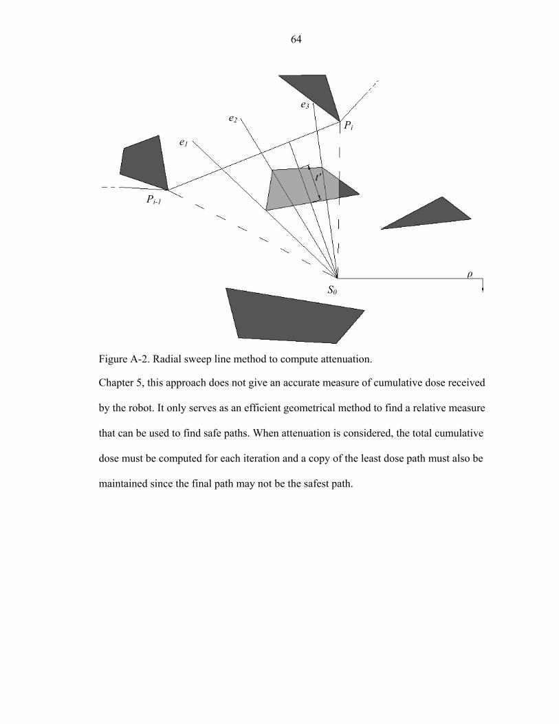
64
e3 e2 Pi
e1
t'
Pi-1
ρ S0
Figure A-2. Radial sweep line method to compute attenuation.
Chapter 5, this approach does not give an accurate measure of cumulative dose received
by the robot. It only serves as an efficient geometrical method to find a relative measure
that can be used to find safe paths. When attenuation is considered, the total cumulative
dose must be computed for each iteration and a copy of the least dose path must also be
maintained since the final path may not be the safest path.
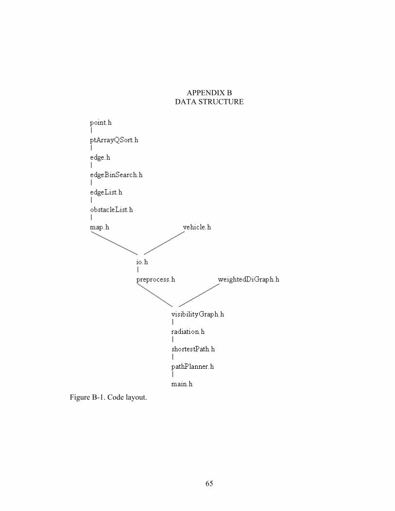
APPENDIX B DATA STRUCTURE
Figure B-1. Code layout.
65
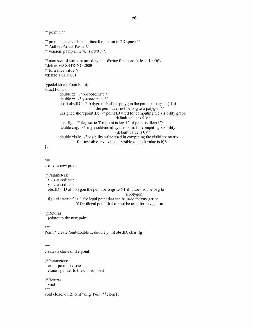
66
/* point.h */ /* point.h declares the interface for a point in 2D space */ /* Author: Arfath Pasha */ /* version: pathplanner4.1 (8/8/01) */ /* max size of string returned by all toString functions (atleast 1000)*/ #define MAXSTRING 2000 /* tolerance value */ #define TOL 0.001 typedef struct Point Point; struct Point { double x; /* x-coordinate */ double y; /* y-coordinate */ short obstID; /* polygon ID of the polygon the point belongs to (-1 if the point does not belong to a polygon */ unsigned short pointID; /* point ID used for computing the visibility graph (default value is 0 )*/ char flg; /* flag set to 'l' if point is legal 'i' if point is illegal */ double ang; /* angle subtended by this point for computing visibility (default value is 0)*/ double visib; /* visibility value used in computing the visibility matrix 0 if invisible, +ve value if visible (default value is 0)*/ }; /** creates a new point @Parameters: x - x-coordinate y - y-coordinate obstID - ID of polygon the point belongs to (-1 if it does not belong to a polygon) flg - character flag 'l' for legal point that can be used for navigation 'i' for illegal point that cannot be used for navigation @Returns: pointer to the new point **/ Point * createPoint(double x, double y, int obstID, char flg) ; /** creates a clone of the point @Parameters: orig - point to clone clone - pointer to the cloned point @Returns: void **/ void clonePoint(Point *orig, Point **clone) ;
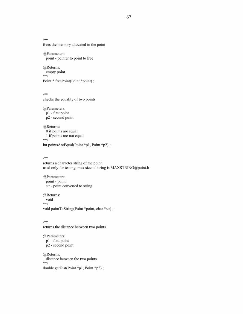
67
/** frees the memory allocated to the point @Parameters: point - pointer to point to free @Returns: empty point **/ Point * freePoint(Point *point) ; /** checks the equality of two points @Parameters: p1 - first point p2 - second point @Returns: 0 if points are equal 1 if points are not equal **/ int pointsAreEqual(Point *p1, Point *p2) ; /** returns a character string of the point. used only for testing. max size of string is [email protected] @Parameters: point - point str - point converted to string @Returns: void **/ void pointToString(Point *point, char *str) ; /** returns the distance between two points @Parameters: p1 - first point p2 - second point @Returns: distance between the two points **/ double getDist(Point *p1, Point *p2) ;
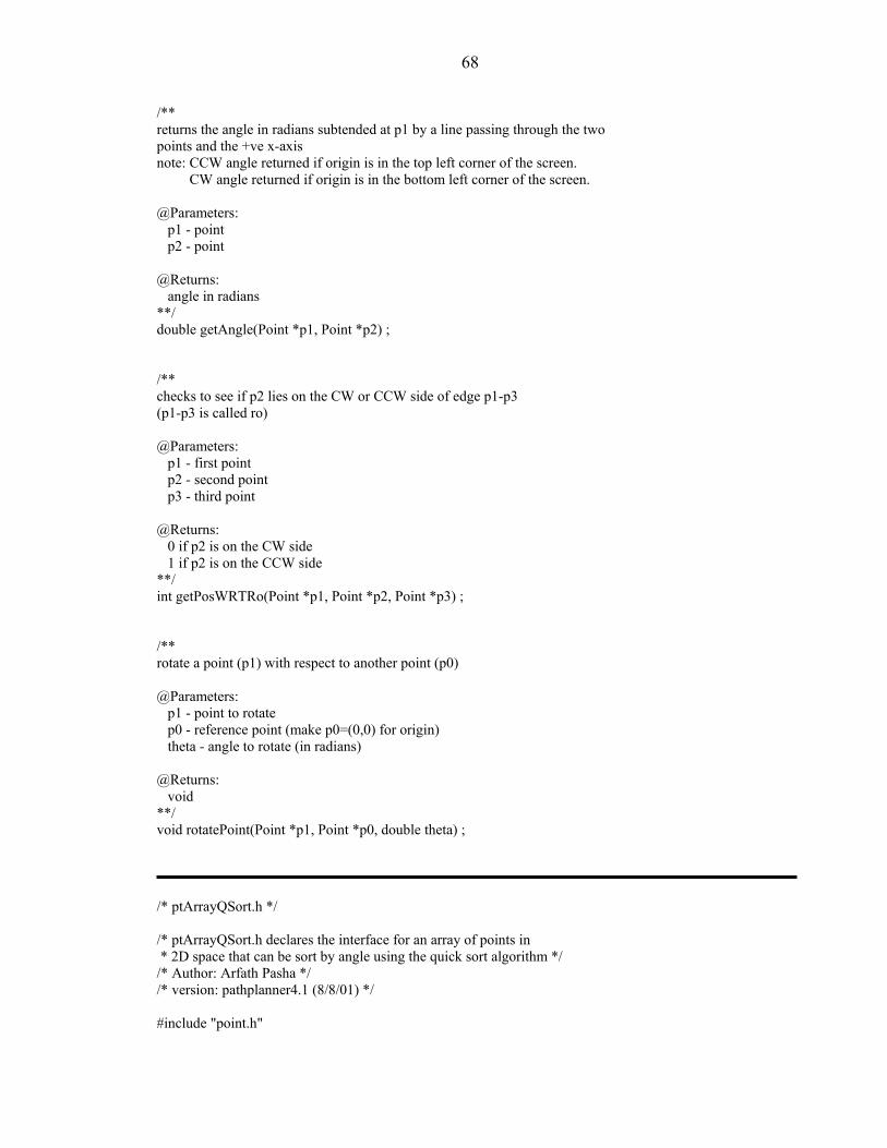
68
/** returns the angle in radians subtended at p1 by a line passing through the two points and the +ve x-axis note: CCW angle returned if origin is in the top left corner of the screen. CW angle returned if origin is in the bottom left corner of the screen. @Parameters: p1 - point p2 - point @Returns: angle in radians **/ double getAngle(Point *p1, Point *p2) ; /** checks to see if p2 lies on the CW or CCW side of edge p1-p3 (p1-p3 is called ro) @Parameters: p1 - first point p2 - second point p3 - third point @Returns: 0 if p2 is on the CW side 1 if p2 is on the CCW side **/ int getPosWRTRo(Point *p1, Point *p2, Point *p3) ; /** rotate a point (p1) with respect to another point (p0) @Parameters: p1 - point to rotate p0 - reference point (make p0=(0,0) for origin) theta - angle to rotate (in radians) @Returns: void **/ void rotatePoint(Point *p1, Point *p0, double theta) ; /* ptArrayQSort.h */ /* ptArrayQSort.h declares the interface for an array of points in * 2D space that can be sort by angle using the quick sort algorithm */ /* Author: Arfath Pasha */ /* version: pathplanner4.1 (8/8/01) */ #include "point.h"
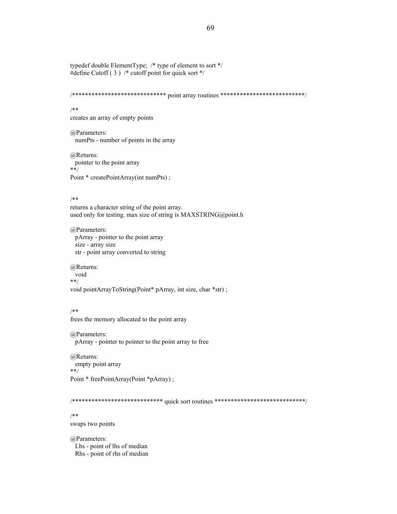
69
typedef double ElementType; /* type of element to sort */ #define Cutoff ( 3 ) /* cutoff point for quick sort */ /***************************** point array routines **************************/ /** creates an array of empty points @Parameters: numPts - number of points in the array @Returns: pointer to the point array **/ Point * createPointArray(int numPts) ; /** returns a character string of the point array. used only for testing. max size of string is [email protected] @Parameters: pArray - pointer to the point array size - array size str - point array converted to string @Returns: void **/ void pointArrayToString(Point* pArray, int size, char *str) ; /** frees the memory allocated to the point array @Parameters: pArray - pointer to pointer to the point array to free @Returns: empty point array **/ Point * freePointArray(Point *pArray) ; /**************************** quick sort routines ****************************/ /** swaps two points @Parameters: Lhs - point of lhs of median Rhs - point of rhs of median
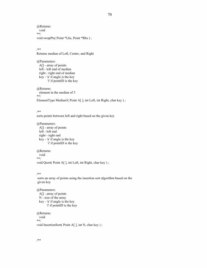
70
@Returns: void **/ void swapPts( Point *Lhs, Point *Rhs ) ; /** Returns median of Left, Center, and Right @Parameters: A[] - array of points left - left end of median right - right end of median key - 'a' if angle is the key 'i' if pointID is the key @Returns: element in the median of 3 **/ ElementType Median3( Point A[ ], int Left, int Right, char key ) ; /** sorts points between left and right based on the given key @Parameters: A[] - array of points left - left end right - right end key - 'a' if angle is the key 'i' if pointID is the key @Returns: void **/ void Qsort( Point A[ ], int Left, int Right, char key ) ; /** sorts an array of points using the insertion sort algorithm based on the given key @Parameters: A[] - array of points N - size of the array key - 'a' if angle is the key 'i' if pointID is the key @Returns: void **/ void InsertionSort( Point A[ ], int N, char key ) ; /**
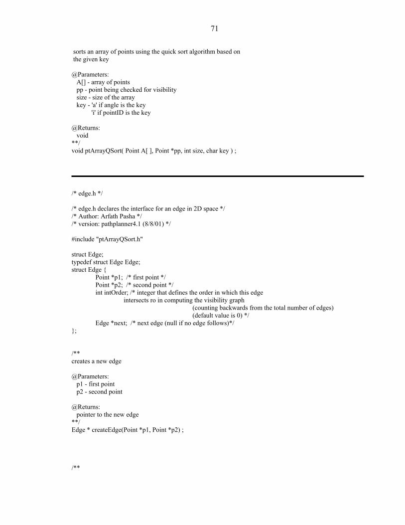
71
sorts an array of points using the quick sort algorithm based on the given key @Parameters: A[] - array of points pp - point being checked for visibility size - size of the array key - 'a' if angle is the key 'i' if pointID is the key @Returns: void **/ void ptArrayQSort( Point A[ ], Point *pp, int size, char key ) ; /* edge.h */ /* edge.h declares the interface for an edge in 2D space */ /* Author: Arfath Pasha */ /* version: pathplanner4.1 (8/8/01) */ #include "ptArrayQSort.h" struct Edge; typedef struct Edge Edge; struct Edge { Point *p1; /* first point */ Point *p2; /* second point */ int intOrder; /* integer that defines the order in which this edge intersects ro in computing the visibility graph (counting backwards from the total number of edges) (default value is 0) */ Edge *next; /* next edge (null if no edge follows)*/ }; /** creates a new edge @Parameters: p1 - first point p2 - second point @Returns: pointer to the new edge **/ Edge * createEdge(Point *p1, Point *p2) ; /**
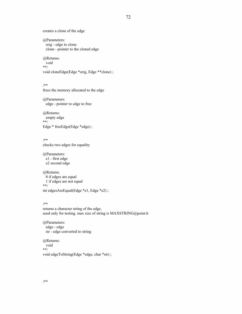
72
creates a clone of the edge @Parameters: orig - edge to clone clone - pointer to the cloned edge @Returns: void **/ void cloneEdge(Edge *orig, Edge **clone) ; /** frees the memory allocated to the edge @Parameters: edge - pointer to edge to free @Returns: empty edge **/ Edge * freeEdge(Edge *edge) ; /** checks two edges for equality @Parameters: e1 - first edge e2 second edge @Returns: 0 if edges are equal 1 if edges are not equal **/ int edgesAreEqual(Edge *e1, Edge *e2) ; /** returns a character string of the edge. used only for testing. max size of string is [email protected] @Parameters: edge - edge str - edge converted to string @Returns: void **/ void edgeToString(Edge *edge, char *str) ; /**
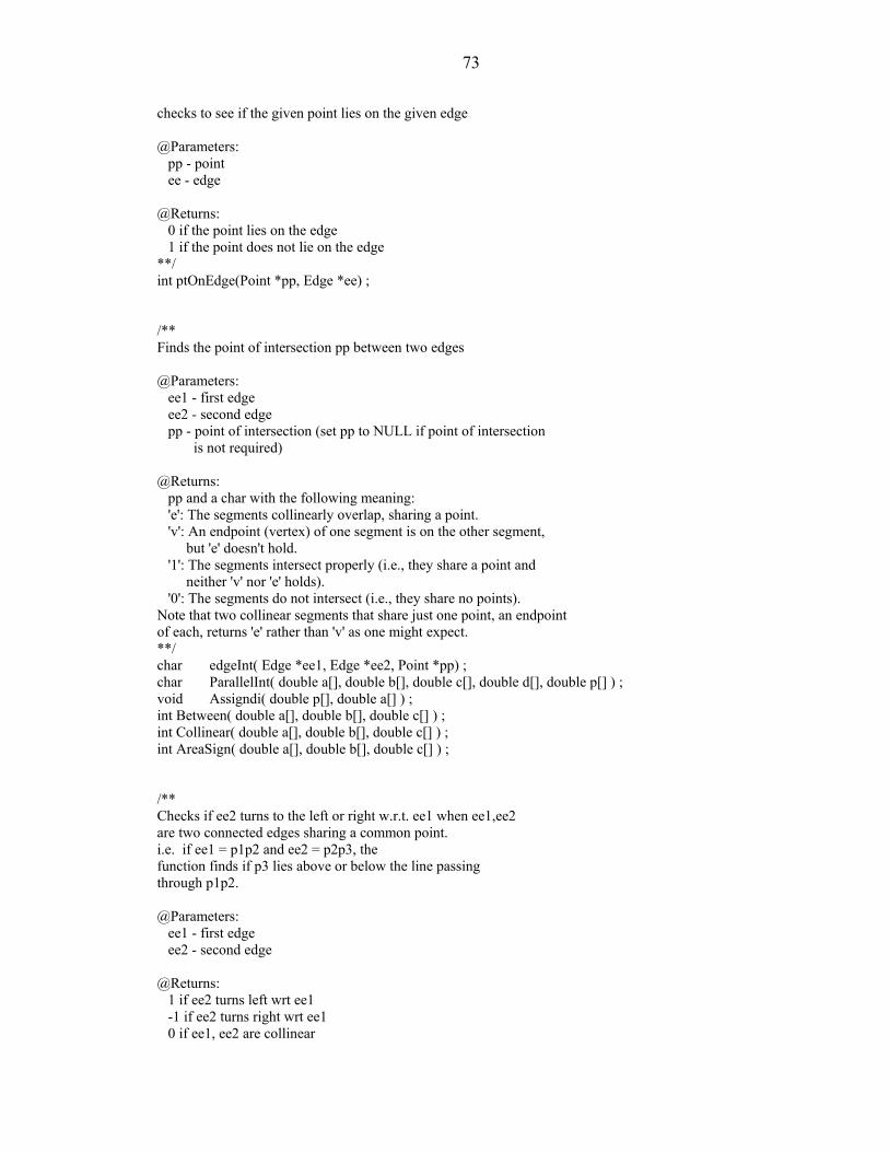
73
checks to see if the given point lies on the given edge @Parameters: pp - point ee - edge @Returns: 0 if the point lies on the edge 1 if the point does not lie on the edge **/ int ptOnEdge(Point *pp, Edge *ee) ; /** Finds the point of intersection pp between two edges @Parameters: ee1 - first edge ee2 - second edge pp - point of intersection (set pp to NULL if point of intersection is not required) @Returns: pp and a char with the following meaning: 'e': The segments collinearly overlap, sharing a point. 'v': An endpoint (vertex) of one segment is on the other segment, but 'e' doesn't hold. '1': The segments intersect properly (i.e., they share a point and neither 'v' nor 'e' holds). '0': The segments do not intersect (i.e., they share no points). Note that two collinear segments that share just one point, an endpoint of each, returns 'e' rather than 'v' as one might expect. **/ char edgeInt( Edge *ee1, Edge *ee2, Point *pp) ; char ParallelInt( double a[], double b[], double c[], double d[], double p[] ) ; void Assigndi( double p[], double a[] ) ; int Between( double a[], double b[], double c[] ) ; int Collinear( double a[], double b[], double c[] ) ; int AreaSign( double a[], double b[], double c[] ) ; /** Checks if ee2 turns to the left or right w.r.t. ee1 when ee1,ee2 are two connected edges sharing a common point. i.e. if ee1 = p1p2 and ee2 = p2p3, the function finds if p3 lies above or below the line passing through p1p2. @Parameters: ee1 - first edge ee2 - second edge @Returns: 1 if ee2 turns left wrt ee1 -1 if ee2 turns right wrt ee1 0 if ee1, ee2 are collinear

74
**/ int turns (Edge *ee1, Edge *ee2); /** Checks if the point common to two connected edges ee1 and ee2 is convex or concave. If ee1 = p1p2 and ee2 = p2p3 in a polygon, the function checks if p2 is a convex point or a concave point. @Parameters: ee1 - first edge ee2 - second edge @Returns: 1 if p2 is a convex point -1 if p2 is a concave point 0 if ee1, ee2 are collinear @note: The polygon is assumed to be oriented counter clockwise. **/ int isConvex (Edge *ee1, Edge *ee2); /* edgeBinSearch.h */ /* edgeArrayWithBinSearch.h declares the interface for the binary search * of edges */ /* Author: Arfath Pasha */ /* version: pathplanner4.1 (8/8/01) */ #include "edge.h" struct TreeNode; typedef struct TreeNode *Position; typedef struct TreeNode *SearchTree; struct TreeNode { Edge *Element; SearchTree Left; SearchTree Right; }; /** frees memory allocated to the search tree @Parameters: T - search tree to free @Returns: pointer to the empty search tree **/
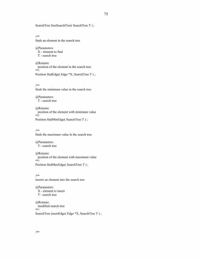
75
SearchTree freeSearchTree( SearchTree T ) ; /** finds an element in the search tree @Parameters: X - element to find T - search tree @Returns: position of the element in the search tree **/ Position findEdge( Edge *X, SearchTree T ) ; /** finds the minimum value in the search tree @Parameters: T - search tree @Returns: position of the element with minimum value **/ Position findMinEdge( SearchTree T ) ; /** finds the maximum value in the search tree @Parameters: T - search tree @Returns: position of the element with maximum value **/ Position findMaxEdge( SearchTree T ) ; /** inserts an element into the search tree @Parameters: X - element to insert T - search tree @Returns: modified search tree **/ SearchTree insertEdge( Edge *X, SearchTree T ) ; /**
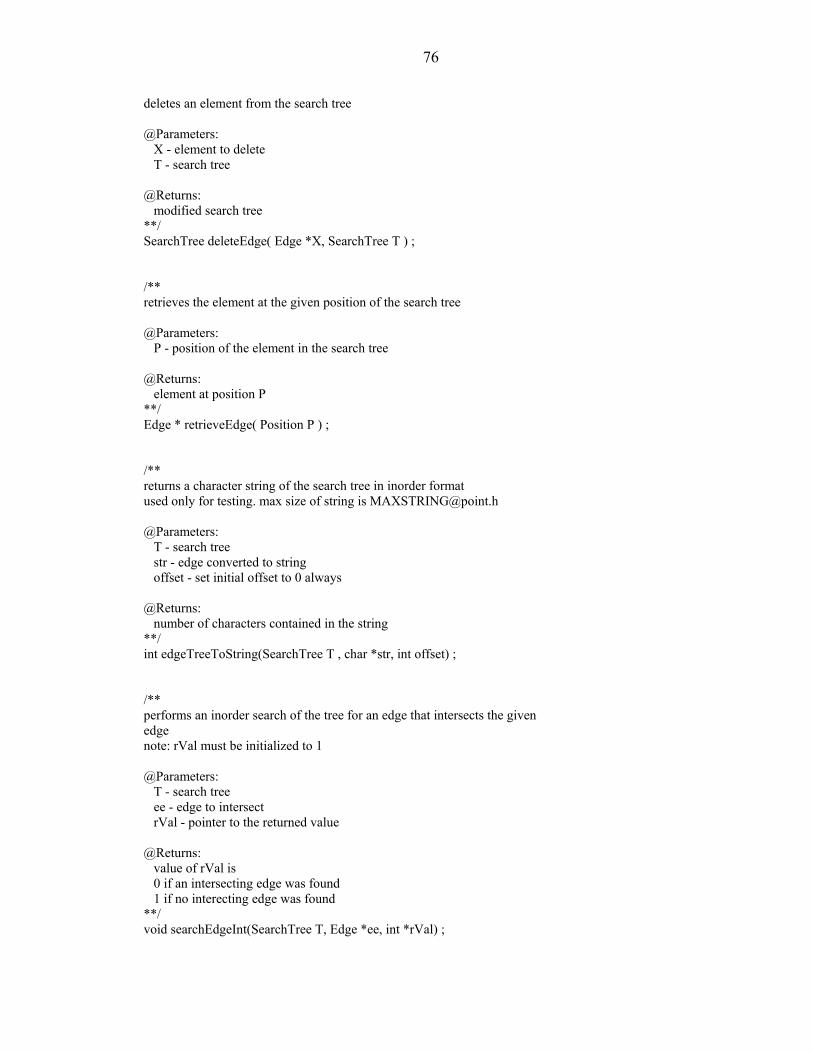
76
deletes an element from the search tree @Parameters: X - element to delete T - search tree @Returns: modified search tree **/ SearchTree deleteEdge( Edge *X, SearchTree T ) ; /** retrieves the element at the given position of the search tree @Parameters: P - position of the element in the search tree @Returns: element at position P **/ Edge * retrieveEdge( Position P ) ; /** returns a character string of the search tree in inorder format used only for testing. max size of string is [email protected] @Parameters: T - search tree str - edge converted to string offset - set initial offset to 0 always @Returns: number of characters contained in the string **/ int edgeTreeToString(SearchTree T , char *str, int offset) ; /** performs an inorder search of the tree for an edge that intersects the given edge note: rVal must be initialized to 1 @Parameters: T - search tree ee - edge to intersect rVal - pointer to the returned value @Returns: value of rVal is 0 if an intersecting edge was found 1 if no interecting edge was found **/ void searchEdgeInt(SearchTree T, Edge *ee, int *rVal) ;
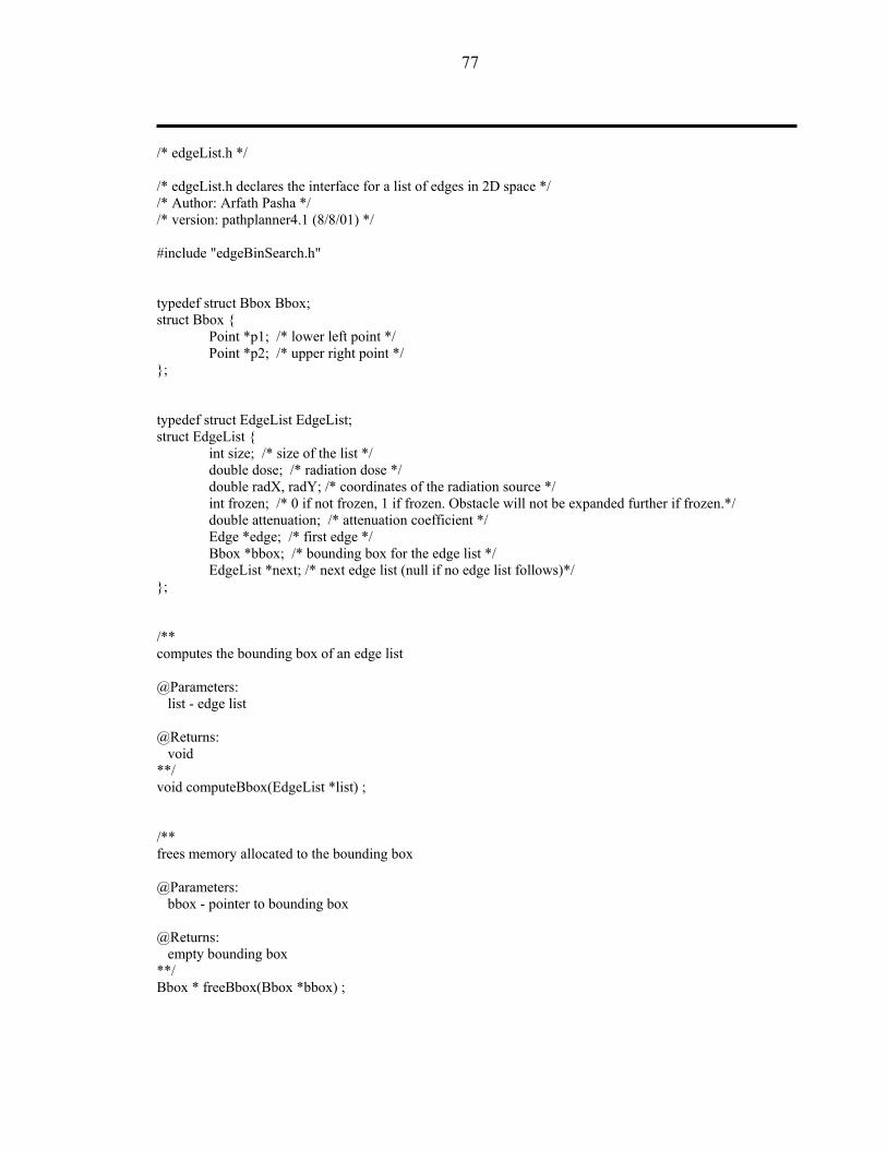
77
/* edgeList.h */ /* edgeList.h declares the interface for a list of edges in 2D space */ /* Author: Arfath Pasha */ /* version: pathplanner4.1 (8/8/01) */ #include "edgeBinSearch.h" typedef struct Bbox Bbox; struct Bbox { Point *p1; /* lower left point */ Point *p2; /* upper right point */ }; typedef struct EdgeList EdgeList; struct EdgeList { int size; /* size of the list */ double dose; /* radiation dose */ double radX, radY; /* coordinates of the radiation source */ int frozen; /* 0 if not frozen, 1 if frozen. Obstacle will not be expanded further if frozen.*/ double attenuation; /* attenuation coefficient */ Edge *edge; /* first edge */ Bbox *bbox; /* bounding box for the edge list */ EdgeList *next; /* next edge list (null if no edge list follows)*/ }; /** computes the bounding box of an edge list @Parameters: list - edge list @Returns: void **/ void computeBbox(EdgeList *list) ; /** frees memory allocated to the bounding box @Parameters: bbox - pointer to bounding box @Returns: empty bounding box **/ Bbox * freeBbox(Bbox *bbox) ;
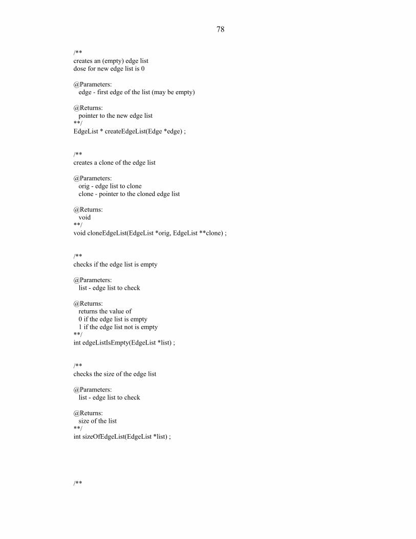
78
/** creates an (empty) edge list dose for new edge list is 0 @Parameters: edge - first edge of the list (may be empty) @Returns: pointer to the new edge list **/ EdgeList * createEdgeList(Edge *edge) ; /** creates a clone of the edge list @Parameters: orig - edge list to clone clone - pointer to the cloned edge list @Returns: void **/ void cloneEdgeList(EdgeList *orig, EdgeList **clone) ; /** checks if the edge list is empty @Parameters: list - edge list to check @Returns: returns the value of 0 if the edge list is empty 1 if the edge list not is empty **/ int edgeListIsEmpty(EdgeList *list) ; /** checks the size of the edge list @Parameters: list - edge list to check @Returns: size of the list **/ int sizeOfEdgeList(EdgeList *list) ; /**
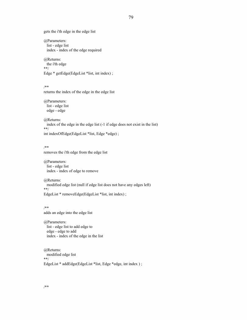
79
gets the i'th edge in the edge list @Parameters: list - edge list index - index of the edge required @Returns: the i'th edge **/ Edge * getEdge(EdgeList *list, int index) ; /** returns the index of the edge in the edge list @Parameters: list - edge list edge - edge @Returns: index of the edge in the edge list (-1 if edge does not exist in the list) **/ int indexOfEdge(EdgeList *list, Edge *edge) ; /** removes the i'th edge from the edge list @Parameters: list - edge list index - index of edge to remove @Returns: modified edge list (null if edge list does not have any edges left) **/ EdgeList * removeEdge(EdgeList *list, int index) ; /** adds an edge into the edge list @Parameters: list - edge list to add edge to edge - edge to add index - index of the edge in the list @Returns: modified edge list **/ EdgeList * addEdge(EdgeList *list, Edge *edge, int index ) ; /**
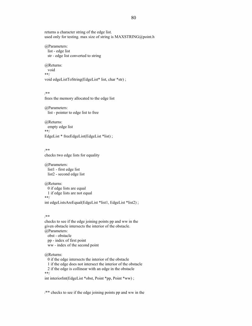
80
returns a character string of the edge list. used only for testing. max size of string is [email protected] @Parameters: list - edge list str - edge list converted to string @Returns: void **/ void edgeListToString(EdgeList* list, char *str) ; /** frees the memory allocated to the edge list @Parameters: list - pointer to edge list to free @Returns: empty edge list **/ EdgeList * freeEdgeList(EdgeList *list) ; /** checks two edge lists for equality @Parameters: list1 - first edge list list2 - second edge list @Returns: 0 if edge lists are equal 1 if edge lists are not equal **/ int edgeListsAreEqual(EdgeList *list1, EdgeList *list2) ; /** checks to see if the edge joining points pp and ww in the given obstacle intersects the interior of the obstacle. @Parameters: obst - obstacle pp - index of first point ww - index of the second point @Returns: 0 if the edge intersects the interior of the obstacle 1 if the edge does not intersect the interior of the obstacle 2 if the edge is collinear with an edge in the obstacle **/ int interiorInt(EdgeList *obst, Point *pp, Point *ww) ; /** checks to see if the edge joining points pp and ww in the
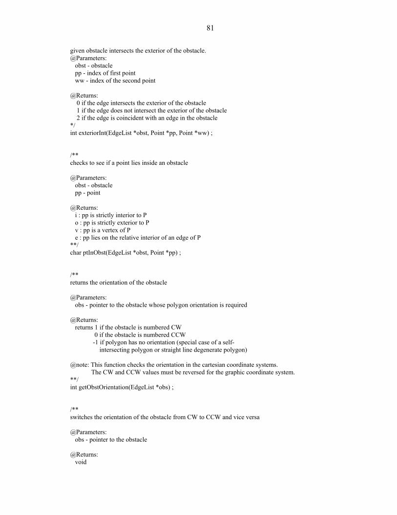
81
given obstacle intersects the exterior of the obstacle. @Parameters: obst - obstacle pp - index of first point ww - index of the second point @Returns: 0 if the edge intersects the exterior of the obstacle 1 if the edge does not intersect the exterior of the obstacle 2 if the edge is coincident with an edge in the obstacle */ int exteriorInt(EdgeList *obst, Point *pp, Point *ww) ; /** checks to see if a point lies inside an obstacle @Parameters: obst - obstacle pp - point @Returns: i : pp is strictly interior to P o : pp is strictly exterior to P v : pp is a vertex of P e : pp lies on the relative interior of an edge of P **/ char ptInObst(EdgeList *obst, Point *pp) ; /** returns the orientation of the obstacle @Parameters: obs - pointer to the obstacle whose polygon orientation is required @Returns: returns 1 if the obstacle is numbered CW 0 if the obstacle is numbered CCW -1 if polygon has no orientation (special case of a self- intersecting polygon or straight line degenerate polygon) @note: This function checks the orientation in the cartesian coordinate systems. The CW and CCW values must be reversed for the graphic coordinate system. **/ int getObstOrientation(EdgeList *obs) ; /** switches the orientation of the obstacle from CW to CCW and vice versa @Parameters: obs - pointer to the obstacle @Returns: void
82
**/ void switchOrientation(EdgeList *obs); /* obstacleList.h */ /* obstacleList.h declares the interface for a list of obstacles in 2D space */ /* Author: Arfath Pasha */ /* version: pathplanner4.1 (8/8/01) */ #include "edgeList.h" typedef struct ObstacleList ObstacleList; struct ObstacleList { int size; /* number of obstacles */ EdgeList *obst; /* list of obstacles */ }; /** creates an (empty) obstacle list @Parameters: obst - first obstacle of the list (may be empty) @Returns: pointer to the new obstacle list **/ ObstacleList * createObstacleList(EdgeList *obst) ; /** creates a clone of the obstacle list @Parameters: orig - obstacle list to clone clone - pointer to cloned obstacle list @Returns: void **/ void cloneObstacleList(ObstacleList *orig, ObstacleList **clone) ; /** frees the memory allocated to the obstacle list @Parameters: list - pointer to obstacle list to free @Returns: empty obstacle list
83
**/ ObstacleList * freeObstacleList(ObstacleList *list) ; /** checks if the obstacle list is empty @Parameters: list - obstacle list to check @Returns: returns the value of 0 if the obstacle list is empty 1 if the obstacle list not is empty **/ int obstacleListIsEmpty(ObstacleList *list) ; /** checks the size of the obstacle list @Parameters: list - obstacle list to check @Returns: size of the list **/ int sizeOfObstacleList(ObstacleList *list) ; /** gets the i'th obstacle in the obstacle list @Parameters: list - obstacle list index - index of the obstacle required @Returns: the i'th obstacle **/ EdgeList * getObstacle(ObstacleList *list, int index) ; /** returns the index of the obstacle in the obstacle list @Parameters: list - obstacle list obst - obstacle @Returns: index of the obstacle in the obstacle list (-1 if obstacle does not exist in the list) **/ int indexOfObstacle(ObstacleList *list, EdgeList *obst) ;
84
/** removes the i'th obstacle from the obstacle list @Parameters: list - obstacle list index - index of obstacle to remove @Returns: modified obstacle list (null if obstacle list does not have any obstacles left) **/ ObstacleList * removeObstacle(ObstacleList *list, int index) ; /** adds an obstacle to the tail of the obstacle list @Parameters: list - obstacle list to add obstacle to obst - obstacle to add @Returns: modified obstacle list **/ ObstacleList * addObstacle(ObstacleList *list, EdgeList *obst) ; /** returns a character string of the obstacle list. used only for testing. max size of string is [email protected] @Parameters: list - obstacle list str - obstale list converted to string @Returns: void **/ void obstacleListToString(ObstacleList* list, char *str) ; /* map.h */ /* map.h declares the interface for a map in 2D space */ /* Author: Arfath Pasha */ /* version: pathplanner4.1 (8/8/01) */ #include "obstacleList.h" typedef struct Map Map;
85
struct Map { ObstacleList *obstList; /* obstacle list */ EdgeList *bdry; /* boundary */ Point *sPt; /* start point */ Point *gPt; /* goal point */ Point *pseudoSPt; /* pseudo start point */ Point *pseudoGPt; /* pseudo goal point */ double sOrient; /* starting orientation of the vehicle (in radians)*/ double gOrient; /* ending orientation of the vehicle (in radians)*/ EdgeList *path; /* shortest path */ short numPts; /* total number of points in the map */ double totalDist; /* distance of the path */ double totalDose; /* Total dose recieved by the vehicle */ }; /** creates a new map for the path planner @Parameters: obstList - obstacle list bdry - boundary sPt - start point gPt - goal point path - shortest path @Returns: pointer to the new map @note: all input paramters must be null if empty **/ Map * createMap(ObstacleList *obstList, EdgeList *bdry, Point *sPt, Point *gPt, EdgeList *path) ; /** frees the memory allocated to the map @Parameters: map - pointer to the map to be freed @Returns: empty map **/ Map * freeMap(Map *map) ; /** returns a character string of the map. used only for testing. max size of string is [email protected] @Parameters:
86
map - map str - map converted to string @Returns: void **/ void mapToString(Map *map, char *str) ; /* vehicle.h */ /* vehicle.h declares the interface for a vehicle */ /* Author: Arfath Pasha */ /* version: pathplanner4.1 (8/8/01) */ typedef struct Vehicle Vehicle; struct Vehicle { double length ; /* vehicle length */ double width ; /* vehicle width */ double speed ; /* vehicle speed */ double tRad ; /* vehicle turning radius */ double gammaAu; /* allowable dose */ }; /** creates a new vehicle @Parameters: length - vehicle length width - vehicle width height - vehicle height tRad - vehicle turning radius gammaAu - allowable dose @Returns: pointer to the new vehicle **/ Vehicle * createVehicle(double length, double width, double speed, double tRad, double gammaAu) ; /** frees the memory allocated to the vehicle @Parameters: vehicle - pointer to vehicle to free @Returns: empty vehicle **/ Vehicle * freeVehicle(Vehicle *vehicle) ;
87
/* weightedDiGraph.h */ /* weightedDiGraph.h declares the interface for a weighted digraph */ /* Author: Arfath Pasha */ /* version: pathplanner4.1 (8/8/01) */ typedef struct WDiGraph WDiGraph; struct WDiGraph { int numPoints; /* number of vertices */ int numEdges; /* number of edges */ double **graph; /* graph implemented as a 2D array */ }; /** creates a new weighted digraph @Parameters: size - size of the weighted digraph @Returns: pointer to the new weighted digraph **/ WDiGraph * createWDiG(int size) ; /** creates a 2D array of the specified size @Parameters: size - size of the array @Returns: pointer to the 2D array **/ double **create2DArray(int size) ; /** puts the edge into the digraph @Parameters: gg - graph ii - first point jj - second point wt - weight of the edge @Returns: void **/ void putEdgeInWDiG(WDiGraph *gg, int ii, int jj, double wt) ;
88
/** returns 0 if edge(i,j) exists. returns 1 otherwise @Parameters: gg - graph ii - first point jj - second point @Returns: 0 if edge exists 1 if edge does not exist **/ int existsEdgeInWDiG(WDiGraph *gg, int ii, int jj) ; /** removes the edge (i,j) @Parameters: gg - graph ii - first point jj - second point @Returns: void **/ void removeEdgeInWDiG(WDiGraph *gg, int ii, int jj) ; /** returns a character string of the weighted digraph. used only for testing. max size of string is [email protected] @Parameters: gg - weighted digraph str - point converted to string @Returns: void **/ void wDiGraphToString(WDiGraph *gg, char *str) ;
LIST OF REFERENCES
1. Rankin AL. Path planning and path execution software for an autonomous nonholonomic robot vehicle [master’s thesis]. Gainesville (FL): University of Florida; 1993.
2. Rao NSV, Kareti S, Shi W, editors. Robot navigation in Unknown Terrains: Introductory Survey of Non-Heuristic Algorithms. Oak Ridge National Laboratory; 1993. Contract No.: ORNL/TM-12410.
3. Reif J, Wang H, The Complexity of the Two Dimensional Curvature Constrained Shortest Path Problem. In: Agarwal PK, Kavraki LE, Mason MT, Karaki LE, editors. Robotics: The Algorithmic Perspective: The Third Workshop on the Algorithmic foundations of Robotics, Natick (MA): A.K. Peters Ltd.; 1998.
4. Informed Consent, U.S. Nuclear Regulatory Commission. 10 C.F.R. Sect. 20.1201 (2002).
5. Chicago Operations Office. 1999. CP-5 Large Scale Demonstration Project. Energy 100 Awards. Available from URL: http://www.ma.doe.gov/energy100/communit/82.html. Site last visited April 2003.
6. Strategic Alliance for Environmental Restoration. 2001. CP-5 Large Scale Demonstration Project. Available from URL: http://www.netl.doe.gov/dd/project_sites/lsddp/cp-5/doc/cp5_website/index.html. Site last visited April 2003.
7. Houssay L. Robotics and Radiation Hardening in the Nuclear Industry [master’s thesis]. Gainesville (FL): University of Florida; 2000.
8. Dubins LE. On Curves of Minimal Length with a Constraint on Average Curvature, and the Prescribed Initial and Terminal Positions and Tangents. American Journal of Mathematics 1957; 79(3): 497-516.
9. Reeds JA, Shepp RA. Optimal Paths for a Car that Goes Both Forward and Backward. Pacific Journal of Mathematics 1991; 145(2): 367-393.
10. Laumond JP, Jacobs PE, Michel T, Murray RM. A Motion Planner for Non-Holonomic Mobile Robots. IEEE Transactions on Robotics and Automation 1994; 10(5): 577-593.
89
90
11. Lafferriere G, Sussman HJ. Motion Planning for Controllable Systems Without Drift: A Preliminary Report. Tech. Report. Busch Campus (NJ): SYSCON-90-04, Rutgers Center for Systems and Control; 1990.
12. Jacob G. Lyndon Discretization of Exact Motion Planning. In: European Controls Conference; 1991; Grenoble, France. p. 1507-1512.
13. Bessiere P, Ahuactzin JM, Talbi EG, Mazer E. The "Ariadne's Clew" Algorithm: Global Planning With Local Methods. In: IEEE Intelligent Robots and Systems Conference; 1993; Yokohama, Japan.
14. Perez TL, Wesley MA, An Algorithm for Planning Collision Free-Paths Among Polyhedral Obstacles. Communications of the ACM 1979; 22(10): 560-570.
15. Nilsson NJ. Problem-solving Methods in Artificial Intelligence. New York (NY): McGraw Hill; 1971.
16. Corman HC, Leiserson CE, Rivest RL, Stein C. Introduction to Algorithms. Cambridge (MA): MIT Press; 2001.
17. Bicchi A, Casalino G, Santilli C. Planning Shortest Bounded-Curvature Paths for a Class of NonHolonomic Vehicles Among Obstacles. Journal of Intelligent and Robotic Systems 1996; 16: 387-405.
18. Asano T, Guibas L, Hershberger J, Imai H. Visibility Polygon Search and Euclidean Shortest Paths. Proceedings of the 26th IEEE Symposium on Foundations of Computer Science; 1985 Oct 21-23; Portland, OR. p. 155-164.
19. Namgung I., Duffy J. Two Dimensional Collision-Free Path Planning Using Linear Parametric Curve. Journal of Robotic Systems 1997; 14(9): 659-673.
20. Brooks RA, Perez TL. A subdivision Algorithm in Configuaration Space for Find-Path with rotation. IEEE Transactions on Systems, Man and Cybernetics 1985; SMC-15(2): 224-233.
21. Zhu D, Latombe JC. New Heuristic Algorithms for Efficient Hierarchical Path Planning. IEEE Transactions on Robotics and Automation 1991; 7(1): 9-20.
22. Suh SH, Shin KG. A Variational Dynamic Programming Approach to Robot-Path Planning with a Distance-Safety Criterion. IEEE Journal of Robotics and Automation 1988; 4(3): 334-349.
23. Wit JS. Vector Pursuit Path Tracking for Autonomous Ground Vehicles [dissertation]. Gainesville (FL): University of Florida; 2000.
24. Fleury S, Sou`eres P, Laumond JP, Chatila R. Primitives for Smoothing Mobile Robot Trajectories. IEEE Transactions on Robotics and Automation 1995; 11: 441-448.
91
25. The Joint Architecture for Unmanned Systems. Reference Architecture Specification, vol. II, Version 3.0, September 13, 2002. Available from URL: http://www.jauswg.org/baseline/current_baseline.shtml. Site last visited April 2003.
26. de Berg M, van Krevald M, Overmars M, Schwarzkopf O. Computational Geometry Algorithms and Applications. Berlin: Springer; 2000.
27. Sahni S. Data Structures Algorithms and Applications in Java. McGraw-Hill; 2000.
28. Kathren RL, editor. A Guide to Reducing Radiation Exposure to as Low as Reasonably Achievable (ALARA). Washington D.C.: Division of Operational & Environmental Safety; 1980. Contract No.: EY-76-C-06-1830. prepared for U.S. Department of Energy, Assistant Secretary for Environment.
29. Evans C, MacArthur D, Novick DK, Pasha A, Zawodny E. UF Eliminator. Final report. Orlando(FL): International Ground Vehicle Competition, AUVSI; 2002.
30. Wood J. Computational Methods in Reactor Shielding. Oxford: Pergamon Press; 1982.

BIOGRAPHICAL SKETCH
Arfath Pasha was born in Bangalore, India, on October 28, 1973. Shortly after
completing his bachelor’s degree at the University of Mysore, India, in mechanical
engineering he attended the University of Florida, Gainesville. Becoming interested in
robotics, he pursued a concurrent master’s degree in mechanical engineering and
computer information science and engineering under the guidance of Dr. Carl D. Crane
III and Dr. Meera Seetharam. During this time he also worked as a graduate research
assistant at the Center for Intelligent Machines and Robotics.
92