computer graphics • path tracing © 2009 fabio pellacini • 1

path tracing

computer graphics • path tracing © 2009 fabio pellacini • 2

path tracing Monte Carlo algorithm for solving the rendering

equation

computer graphics • path tracing © 2009 fabio pellacini • 3

solving rendering equation

•  advantages –  predictive simulation

•  can be used for architecture, engineering, …

–  photorealistic •  if simulation if correct, images will look real

•  disadvantages –  (really) slow

•  simulation of physics is computationally very expensive

–  need accurate geometry, materials and lights •  otherwise just a correct solution to the wrong problem

computer graphics • path tracing © 2009 fabio pellacini • 4

rendering equation

[Bal

a]

x x

computer graphics • path tracing © 2009 fabio pellacini • 5

basic path tracing

•  need to evaluate radiance at x in direction Θ

•  determine visible point

•  look up emission

[Bal

a]

computer graphics • path tracing © 2009 fabio pellacini • 6

basic path tracing

•  need to evaluate

•  use Monte Carlo estimation

computer graphics • path tracing © 2009 fabio pellacini • 7

basic path tracing

•  generate random direction Ψi with p(Ψi)

–  evaluate BRDF –  evaluate cosine –  evaluate

[Bal

a]

computer graphics • path tracing © 2009 fabio pellacini • 8

basic path tracing

•  need to evaluate

•  determine visible point from x in direction Ψi

•  in vacuum

[Bal

a]

computer graphics • path tracing © 2009 fabio pellacini • 9

basic path tracing

•  need to evaluate

•  recursively execute procedure

[Bal

a]

computer graphics • path tracing © 2009 fabio pellacini • 10

russian roulette

•  when to stop recursion? –  light bounce infinitely in the environment –  but every bounce has less energy

•  in many cases 3-4 bounces are enough

[Bal

a]

computer graphics • path tracing © 2009 fabio pellacini • 11

russian roulette

•  stop after k bounces –  introduces bias (consistent error) in the solution –  need to make k large to capture all cases

•  Monte Carlo strategy (Russian Roulette) as stopping criterion –  pick a probability with which to stop the path –  at each intersection, test the path –  correct the radiance estimator accordingly

computer graphics • path tracing © 2009 fabio pellacini • 12

russian roulette

[Dut

ré, B

ekae

rt, B

ala]

computer graphics • path tracing © 2009 fabio pellacini • 13

russian roulette

computer graphics • path tracing © 2009 fabio pellacini • 14

russian roulette

•  if f is a recursive integral, only continue with probability •  but weight back the radiance

•  example: path tracing with –  only 1 chance in 10 the ray will continue –  estimate radiance of the ray multiplies by 10 –  intuition: instead of shooting 10 rays, shoot 1 but weight its

contribution 10 times

computer graphics • path tracing © 2009 fabio pellacini • 15

russian roulette

•  how to choose the probability? –  small fixed value: longer paths

•  slow but accurate

–  big fixed value: shorter paths •  fast but inaccurate

–  proportional to integral of reflected light •  adapts to material properties •  darker patches will statistically shorten paths •  exactly like in physics

computer graphics • path tracing © 2009 fabio pellacini • 16

basic path tracing pseudocode

computeImage() foreach pixel (i,j) estimatedRadiance[i,j] = 0 for s = 1 to #viewSamples generate Q in pixel (i,j) theta = (Q – E)/|Q-E| x = trace(E,theta) estimatedRadiance [i,j] += computeRadiance(x,-theta) estimatedRadiance [i,j] /= #viewSamples

computeRadiance(x, theta) estimatedRadiance = basicPT(x, theta) return estimatedRadiance

[Dut

ré, B

ekae

rt, B

ala]

computer graphics • path tracing © 2009 fabio pellacini • 17

basic path tracing pseudocode

basicPT(x, theta) estimatedRadiance = Le(x, theta) if(not absorbed) // russian roulette for s = 1 to #radianceSamples psi = generate random dir on hemisphere y = trace(x, psi) estimatedRadiance += basicPT(y,-psi) * BRDF(x,psi,theta) * cos(Nx,psi) / pdf(psi) estimatedRadiance /= #paths return estRadiance/(1-absorption)

[Dut

ré, B

ekae

rt, B

ala]

computer graphics • path tracing © 2009 fabio pellacini • 18

basic path tracing intuition

[Dut

ré, B

ekae

rt, B

ala]

computer graphics • path tracing © 2009 fabio pellacini • 19

basic path tracing intuition

[Dut

ré, B

ekae

rt, B

ala]

computer graphics • path tracing © 2009 fabio pellacini • 20

basic path tracing performance

[Bal

a]

1 sample 16 samples 256 samples

computer graphics • path tracing © 2009 fabio pellacini • 21

monte carlo vs. deterministic integration

Monte Carlo Deterministic

[Bal

a]

computer graphics • path tracing © 2009 fabio pellacini • 22

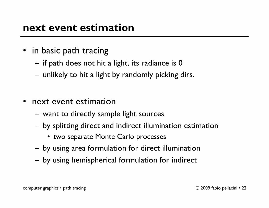
next event estimation

•  in basic path tracing –  if path does not hit a light, its radiance is 0 –  unlikely to hit a light by randomly picking dirs.

•  next event estimation –  want to directly sample light sources –  by splitting direct and indirect illumination estimation

•  two separate Monte Carlo processes

–  by using area formulation for direct illumination –  by using hemispherical formulation for indirect

computer graphics • path tracing © 2009 fabio pellacini • 23

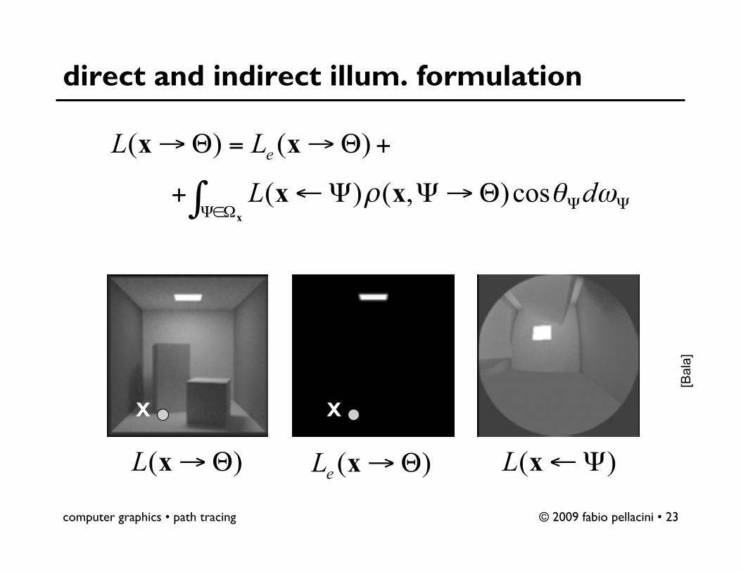
direct and indirect illum. formulation

[Bal

a]

x x

computer graphics • path tracing © 2009 fabio pellacini • 24

direct and indirect illum. formulation

[Bal

a]

computer graphics • path tracing © 2009 fabio pellacini • 25

direct and indirect illum. formulation

computer graphics • path tracing © 2009 fabio pellacini • 26

direct illum. – hemisphere sampling

[Dut

ré, B

ekae

rt, B

ala]

computer graphics • path tracing © 2009 fabio pellacini • 27

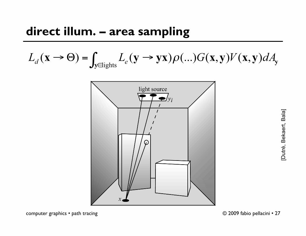
direct illum. – area sampling

[Dut

ré, B

ekae

rt, B

ala]

computer graphics • path tracing © 2009 fabio pellacini • 28

indirect illum. – hemisphere sampling

[Dut

ré, B

ekae

rt, B

ala]

discard Le if ray hits light

computer graphics • path tracing © 2009 fabio pellacini • 29

indirect illum. – recursive evaluation

[Dut

ré, B

ekae

rt, B

ala]

computer graphics • path tracing © 2009 fabio pellacini • 30

next event estimation performance

[Bal

a]

16 samples

without with

computer graphics • path tracing © 2009 fabio pellacini • 31

next event estimation performance

[Bal

a]

16 samples

1 sample 4 samples

256 samples

computer graphics • path tracing © 2009 fabio pellacini • 32

direct illumination – one light

•  depends on –  emitted radiance distribution Le –  how to pick points y on the light –  how many points to use

•  number of shadow rays

computer graphics • path tracing © 2009 fabio pellacini • 33

direct illumination – one light

•  each light type has its own physical models –  angular distribution defines different light types –  flood, fill, spot, ect…

•  simplest model: emitted radiance is a constant

computer graphics • path tracing © 2009 fabio pellacini • 34

direct illumination – one light

•  uniform sampling of light area

–  simply sample that [0,1] square and rescale –  works fairly well in practice –  slightly better techniques exists tough

computer graphics • path tracing © 2009 fabio pellacini • 35

direct illumination – many lights

[Dut

ré, B

ekae

rt, B

ala]

computer graphics • path tracing © 2009 fabio pellacini • 36

direct illumination – many lights

•  how to allocate samples between different lights –  various techniques, some quite advanced

computer graphics • path tracing © 2009 fabio pellacini • 37

direct illumination – many lights

•  split samples uniformly between lights –  same as M light integrals with previous sampling

–  simple but inefficient •  would like to weight more brighter lights •  won’t cover in this class

computer graphics • path tracing © 2009 fabio pellacini • 38

indirect illumination

•  depends on how to sample the hemisphere –  uniform distribution –  importance sampling: pick p to match integral

•  cosine distribution •  BRDF distribution •  BRDF*cosine distribution

computer graphics • path tracing © 2009 fabio pellacini • 39

indirect illumination – uniform dist.

[Bal

a]

computer graphics • path tracing © 2009 fabio pellacini • 40

indirect illumination – cosine dist.

[Bal

a]

computer graphics • path tracing © 2009 fabio pellacini • 41

indirect illumination – BRDF Dist.

[Bal

a]

computer graphics • path tracing © 2009 fabio pellacini • 42

indirect illumination – BRDF*Cosine Dist.

[Bal

a]

computer graphics • path tracing © 2009 fabio pellacini • 43

importance sampling performance

[Bal

a]

without with

computer graphics • path tracing © 2009 fabio pellacini • 44

pt pseudocode – pixel sampling

computeImage() foreach pixel (i,j) estimatedRadiance[i,j] = 0 for s = 1 to #viewSamples generate Q in pixel (i,j) theta = (Q – E)/|Q-E| x = trace(E,theta) estimatedRadiance [i,j] += computeRadiance(x,-theta) estimatedRadiance [i,j] /= #viewSamples [D

utré

, Bek

aert,

Bal

a]

computer graphics • path tracing © 2009 fabio pellacini • 45

pt pseudocode – radiance estimation

computeRadiance(x,theta) estimatedRadiance = Le(x,theta) estimatedRadiance += directIllumination(x, theta) estimatedRadiance += indirectIllumination(x, theta) return estimatedRadiance

[Dut

ré, B

ekae

rt, B

ala]

computer graphics • path tracing © 2009 fabio pellacini • 46

pt pseudocode – direct illumination

directIllumination(x,theta) estimatedRadiance = 0 for s = 1 to #shadowRays k = pick random light y = generate random point on light k psi = (x-y) / |x-y| estimatedRadiance += Le_k(y,-psi) * BRDF(x,psi,tetha) * G(x,y) * V(x,y) / (p(k)*p(y|k)) estimateRadiance /= #shadowRays return estimatedRadiance

[Dut

ré, B

ekae

rt, B

ala]

computer graphics • path tracing © 2009 fabio pellacini • 47

pt pseudocode – direct illumination UL

directIllumination(x,theta) estimatedRadiance = 0 for k = 1 to #lights for s = 1 to #shadowRays / #lights y = generate random point on light k psi = (x-y) / |x-y| estimatedRadiance += Le_k(y,-psi) * BRDF(x,psi,tetha) * G(x,y) * V(x,y) / p(y) estimateRadiance /= #shadowRays return estimatedRadiance

[Dut

ré, B

ekae

rt, B

ala]

computer graphics • path tracing © 2009 fabio pellacini • 48

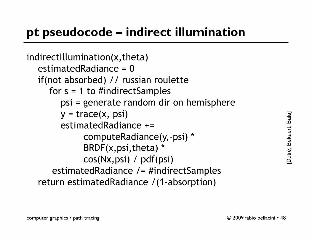
pt pseudocode – indirect illumination

indirectIllumination(x,theta) estimatedRadiance = 0 if(not absorbed) // russian roulette for s = 1 to #indirectSamples psi = generate random dir on hemisphere y = trace(x, psi) estimatedRadiance += computeRadiance(y,-psi) * BRDF(x,psi,theta) * cos(Nx,psi) / pdf(psi) estimatedRadiance /= #indirectSamples return estimatedRadiance /(1-absorption)

[Dut

ré, B

ekae

rt, B

ala]

computer graphics • path tracing © 2009 fabio pellacini • 49

beyond path tracing bidirectional techniues

computer graphics • path tracing © 2009 fabio pellacini • 50

path tracing

•  perfectly accurate, but slow to converge –  noise remains in the image for a long time

•  intuition: is there are bright reflections, we cannot sample them directly –  halogen lamps

•  idea: shoot paths from the eye and from the light –  eye paths: work well for reflections –  light paths: pick up secondary sources –  in reality very complex

computer graphics • path tracing © 2009 fabio pellacini • 51

bidirectional path tracing

[Dut

ré, B

ekae

rt, B

ala]

computer graphics • path tracing © 2009 fabio pellacini • 52

bidirectional path tracing

[Dut

ré, B

ekae

rt, B

ala]

computer graphics • path tracing © 2009 fabio pellacini • 53

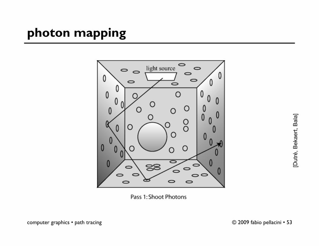
photon mapping

[Dut

ré, B

ekae

rt, B

ala]

computer graphics • path tracing © 2009 fabio pellacini • 54

photon mapping

[Dut

ré, B

ekae

rt, B

ala]