Patient scheduling based on a service-time prediction

Noname manuscript No.(will be inserted by the editor)

Patient scheduling based on a service-time prediction model:A data-driven study for a radiotherapy center

Dina Ben Tayeb · Nadia Lahrichi · Louis-Martin Rousseau

Received: date / Accepted: date

Abstract With the growth of the population, access to

medical care is in high demand, and queues are becom-

ing longer. The situation is more critical when it con-

cerns serious diseases such as cancer. The primary prob-

lem is inefficient management of patients rather than a

lack of resources. In this work, we collaborate with the

Centre Integre de Cancerologie de Laval (CICL). We

present a data-driven study based on a nonblock ap-

proach to patient appointment scheduling. We use data

mining and regression methods to develop a prediction

model for radiotherapy treatment duration. The best

model is constructed by a classification and regression

tree; its accuracy is 84%. Based on the predicted dura-

tion, we design new workday divisions, which are evalu-

ated with various patient sequencing rules. The results

show that with our approach, 40 additional patients aretreated daily in the cancer center, and a considerable

improvement is noticed in patient waiting times and

technologist overtime.

Keywords Patient scheduling · Data-driven ap-

proach · Prediction models · Nonblock scheduling ·Grid design · Sequencing rules

D. Ben Tayeb · N. Lahrichi · L.-M. RousseauDepartment of Mathematical and Industrial Engineering,CIRRELT and Polytechnique Montreal, C.P. 6079,Succursale Centre-ville, Montreal, QC,Canada, H3C 3A7E-mail: [email protected]

N. LahrichiE-mail: [email protected]

L.-M. RousseauE-mail: [email protected]

1 Introduction

Nearly half of all Canadians will be diagnosed with can-

cer during their lifetime. Cancer is the leading cause of

death in Canada [1]. These statistics indicate that it is

vital to ensure timely access to medical care. However,

given the continued growth in the number of cancer pa-

tients, an imbalance between appointment demand and

treatment capacity has arisen. Therefore, waiting times

are becoming longer. This leads to patient dissatisfac-

tion and higher costs for clinics. The critical factor is

usually suboptimal patient scheduling rather than lim-

ited resources. To face these challenges, cancer centers

must better manage patient appointments. In this pa-

per, we a present data-driven study that develops de-

cision support tools based on data mining to improve

patient scheduling. We collaborate with the department

of radiotherapy at the Centre Integre de Cancerologie

de Laval (CICL).

The decisions involved in planning an outpatient ap-

pointment system can be classified into three categories:

strategic, tactical, and operational [2]. We consider the

tactical and operational levels separately and sequen-

tially. The tactical level includes the development of a

more reliable appointment interval, which directly im-

pacts the number of appointments in a session. The

operational level involves determining the patient ap-

pointment times according to a given sequencing rule.

There are two appointment scheduling strategies:

block and nonblock systems [10]. The block system di-

vides the day into a fixed number of slots with the same

duration, whereas the nonblock system allows appoint-

ment intervals of different durations. The CICL uses

a block policy. Radiotherapy appointment scheduling

is complex, since the treatment is divided into several

sessions that occur on successive days, and the CICL

2 Patient scheduling based on a service-time prediction model

requires all the treatments for a patient to take place at

the same time of day and in the same room. Therefore,

it is simpler to apply the block strategy. However, most

of the allocated slots are not respected; the service time

differs from one patient to another.

Appointment management systems that allocate uni-

form slots assume that patients are similar, and all the

treatments have a given average duration that deter-

mines the length of the appointment interval. In reality,

the patients differ in terms of disease category and man-

agement, and even the features of the visits vary (the

first treatment or the last, the patient arrives from the

emergency room or the hospital, etc.). Several factors

affect the patient service time, so it is sensible to allow

considerable variation in these durations. In the block

scheduling system, treatments that end early compen-

sate for others that exceed the expected time. However,

the lack of control of the service-time variability gener-

ates indirect costs related to capacity underutilization,

overtime, and waiting time.

This paper develops a data-driven approach to ef-

ficient appointment scheduling based on the nonblock

strategy. The method has two phases. The first phase

(Section 3) predicts the patient service time based on

the treatment characteristics. We apply data mining

and regression tools to extract information from med-

ical data. The main goal is to classify patients accord-

ing to their treatment durations. The prediction algo-

rithm must be very accurate in order to lead to effec-

tive patient scheduling. The second phase (Section 4) is

a patient appointment system based on the prediction

model. We design the appointment grid and determine

patient management and sequencing rules. Reliable pa-

tient service times lead to better scheduling; we aim to

maximize the outpatient clinic utilization and minimize

the patient waiting time and the technologist overtime.

To the best of our knowledge, this work is the first

radiotherapy application that uses data mining and re-

gression methods to define patient appointment dura-

tions and proceeds to develop a more efficient patient

schedule based on the nonblock strategy. It is a data-

driven study that uses real CICL Radiotherapy data.

The steps are as follows: current scheduling strategy

analysis; extraction of actionable models; development

of patient schedule; determination of patient sequenc-

ing and operational management rules; evaluation; and

validation. Compared to the current scheduling system,

our approach gives good results in terms of waiting

time, overtime, and the number of patients seen per

day; the improvement reaches 30%.

The remainder of the paper is organized as follows.

Section 2 summarizes related work and gives the prob-

lem statement. Section 3 discusses the development of

our prediction model for the service time. Section 4 dis-

cusses the development of the appointment scheduling

system and the results. Finally, Section 5 provides con-

cluding remarks.

2 Problem statement and related work

The CICL workday is split into a fixed number of 20 min

appointments. However, the actual treatment time may

vary, so for many patients the appointment times are

not respected. They can either arrive early or risk wait-

ing a long time. Figure 1 shows that the median waiting

times in September 2017 ranged from 0 to 8 min, with

the largest variability on day 28.

Fig. 1 Patient waiting times in September 2017.

The CICL has four active rooms with linear ac-

celerators, and 32 patients can be treated per day in

each room. However, the demand may exceed this limit.

Also, technologists may finish early or work overtime.

Our goal is to develop an efficient patient scheduling

method. Outpatient appointment scheduling has been

widely studied, starting with the pioneering work of [4].

Three reviews [8,16,2] provide a global overview of de-

velopments. Cayirli & Veral [8] present various formula-

tions based on mathematical programming, simulation,

and queuing theory. Gupta & Denton [16] define differ-

ent types of health care systems, focusing on the factors

that complicate appointment scheduling. Ahmadi-Javid

et al. [2] classify the scheduling decisions into three

classes: strategic, tactical, and operational.

Cayirli et al. [9] show that appointment schedul-

ing systems can be improved by classifying the pa-

tients according to, e.g., the type of procedure required

or the variability of the service time. They differenti-

ate between new and returning patients. Based on this

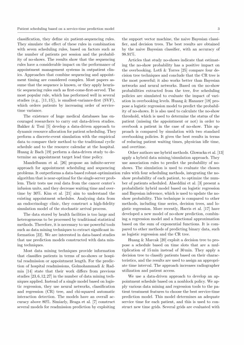
Patient scheduling based on a service-time prediction model 3

classification, they define six patient-sequencing rules.

They simulate the effect of these rules in combination

with seven scheduling rules, based on factors such as

the number of patients per session and the probabil-

ity of no-shows. The results show that the sequencing

rules have a considerable impact on the performance of

appointment management systems in outpatient clin-

ics. Approaches that combine sequencing and appoint-

ment timing are considered complex. Most papers as-

sume that the sequence is known, or they apply heuris-

tic sequencing rules such as first-come-first-served. The

most popular rule, which has performed well in several

studies (e.g., [11,15]), is smallest-variance-first (SVF),

which orders patients by increasing order of service-

time variance.

The existence of huge medical databases has en-

couraged researchers to carry out data-driven studies.

Bakker & Tsui [5] develop a data-driven approach to

dynamic resource allocation for patient scheduling. They

perform a discrete-event simulation with the empirical

data to compare their method to the traditional cyclic

schedule and to the resource calendar at the hospital.

Huang & Bach [19] perform a data-driven study to de-

termine an appointment target lead time policy.

Mandelbaum et al. [26] propose an infinite-server

approach for appointment scheduling and sequencing

problems. It outperforms a data-based robust-optimization

algorithm that is near-optimal for the single-server prob-

lem. Their tests use real data from the cancer center’s

infusion units, and they decrease waiting time and over-

time by 30%. Kim et al. [21] aim to understand the

existing appointment schedules. Analyzing data from

an endocrinology clinic, they construct a high-fidelity

simulation model of the stochastic arrival process.

The data stored by health facilities is too large and

heterogeneous to be processed by traditional statistical

methods. Therefore, it is necessary to use powerful tools

such as data mining techniques to extract significant in-

formation [22]. We are interested in data-based studies

that use prediction models constructed with data min-

ing techniques.

Most data mining techniques provide information

that classifies patients in terms of no-shows or hospi-

tal readmission or appointment length. For the predic-

tion of hospital readmissions, Golmohammadi & Rad-

mia [14] state that their work differs from previous

studies [23,6,12,27] in the number of data mining tech-

niques applied. Instead of a single model based on logis-

tic regression, they use neural networks, classification

and regression (CR) tree, and chi-squared automatic

interaction detection. The models have an overall ac-

curacy above 80%. Simiarly, Braga et al. [7] construct

several models for readmission prediction by exploiting

the support vector machine, the naive Bayesian classi-

fier, and decision trees. The best results are obtained

by the naive Bayesian classifier, with an accuracy of

98.91%.

Articles that study no-shows indicate that estimat-

ing the no-show probability has a positive impact on

the overbooking. Lotfi & Torres [25] compare four de-

cision tree techniques and conclude that the CR tree is

the most powerful; it also works better than Bayesian

networks and neural networks. Based on the no-show

probabilities extracted from the tree, five scheduling

policies are simulated to evaluate the impact of vari-

ation in overbooking levels. Huang & Hanauer [18] pro-

pose a logistic regression model to predict the probabil-

ity of no-shows. It is also used to calculate the no-show

threshold, which is used to determine the status of the

patient (missing the appointment or not) in order to

overbook a patient in the case of no-show. This ap-

proach is compared by simulation with two standard

overbooking policies. It gives the best results in terms

of reducing patient waiting times, physician idle time,

and overtime.

Other authors use hybrid methods. Glowacka et al. [13]

apply a hybrid data mining/simulation approach. They

use association rules to predict the probability of no-

shows. The simulation is used to evaluate the chosen

rules with four scheduling methods, integrating the no-

show probability of each patient, to optimize the num-

ber of patients scheduled. Alaeddini et al. [3] present a

probabilistic hybrid model based on logistic regression

and Bayesian inference, which is used to update the no-

show probability. This technique is compared to other

methods, including time series, decision trees, and lo-

gistic regression. More recently, Harris et al. [17] have

developed a new model of no-show prediction, combin-

ing a regression model and a functional approximation

based on the sum of exponential functions. It is com-

pared to other methods of predicting binary data, such

as logistic regression and the CR tree.

Huang & Marcak [20] exploit a decision tree to pro-

pose a schedule based on time slots that are a mul-

tiplication of 15 min instead of 30 min. They apply a

decision tree to classify patients based on their charac-

teristics, and the results are used to assign an appropri-

ate time interval. The approach increases radiographer

utilization and patient access.

We use a data-driven approach to develop an ap-

pointment schedule based on a nonblock policy. We ap-

ply various data mining and regression tools to the pa-

tient treatment features to choose the best service-time

prediction model. This model determines an adequate

service time for each patient, and this is used to con-

struct new time grids. Several grids are evaluated with


different patient sequencing and management rules to

select the best appointment system.

3 Development of the prediction model

In this section, we develop a tool for predicting the pa-

tient treatment times. The service or treatment time

represents the total time during which the technolo-

gists interact with and treat a patient during a given

session. The prediction model must be very accurate in

order to lead to efficient patient scheduling. Thus, sev-

eral prediction methods are compared. We work with

real data from CICL Radiotherapy. This study follows

the CRISP-DM process (CRoss Industry Standard Pro-

cess for Data Mining).

3.1 Data mining process

Larose & Larose [24] present data mining as a well-

structured standard process. They claim that every data

mining project follows the CRISP-DM, which has six

phases (see Fig. 2):

1. Business understanding: The first phase expresses

objectives and prepares a strategy to achieve them.

2. Data understanding: This phase collects the data

and evaluates their quality. It also identifies inter-

esting subsets that may contain actionable models.

3. Data preparation: This phase cleans the raw data,

selects attributes to analyze, and performs any nec-

essary variable transformations.

4. Modeling: Several modeling techniques can be used.

During this phase, the data may be adapted for a

specific data mining method.

5. Evaluation: This phase evaluates the quality and ef-

fectiveness of the models from the previous phase.

6. Deployment: The project does not end with the cre-

ation of the model. It must be further developed and

adapted according to the customer’s needs.

3.2 Application of the CRISP-DM to CICL service

time prediction

3.2.1 Business understanding

The goal of this study is to predict the service time for

radiotherapy patients based on their treatment charac-

teristics, and to identify the important variables that

provide this information.

Fig. 2 CRoss Industry Standard Process for Data Mining(CRISP-DM).

3.2.2 Data understanding

The data correspond to treatments performed at the

CICL from 2012 to 2016. They include information re-

lated to the patient’s visit (date of appointment, start

time and end time, etc.), and treatment features (cate-

gory, room, etc.).

At this step, it is essential to perform a descriptive

analysis to gain a clear idea of the current state. We

start by verifying the accuracy of the allocated service

time. Figure 3 shows that the average treatment time

ranges from 2 to 22 min, but all the appointment in-

tervals are the same (20 min). Adjusting the durations

could lead to better patient scheduling.

Fig. 3 Average treatment times in CICL.

We therefore analyze the treatment attributes (can-

cer category, care plan, status, and treatment room)

and their impact on the treatment duration. Figure 4

indicates that the main cancer types are breast and

prostate cancer. Figure 5 shows that most cancers have

a treatment time between 10 and 12 min. Cancers of the

vulva and anal canal require more time, whereas semi-

noma, brain, and sinus cancer are treated more quickly.

Figure 6 shows that these cancers also have the short-


est average treatment time by care plan. Figure 7 shows

the average treatment time by status; this combines in-

formation about the patient and the treatment session.

The status indicates, e.g., if the patient is hospitalized

(H), if there is a change of treatment plan (PS), and

if the session is the first (DC) or last (FC). The first

treatment usually takes more time. Figure 8 indicates

that the average treatment time is almost the same for

all the rooms.

Fig. 4 Cancer categories in CICL.

Fig. 5 Average treatment times by cancer category.

3.2.3 Data preparation

This phase consists of cleaning the data, adding new

attributes, and preparing and selecting the attributes.

Data cleaning We start by removing unnecessary in-

formation and outliers or incorrect data. Negative or

excessively long periods are also removed. This elimi-

nates less than 3% of the data.

Fig. 6 Average treatment times by care plan.

Fig. 7 Average treatment times by status.

Fig. 8 Average treatment times by room.

Attribute addition We calculate the treatment dura-

tion, which starts at the moment that the patient enters

the treatment room, and then find the average duration.

Attribute preparation Because we plan to design a stan-

dard appointment grid, we convert the continuous out-

put into a categorical variable with the following classes:

5, 10, 15, 20, and 25 min.

Attribute selection This step identifies the important

attributes. We used the chi-square test χ2, which is a

statistical test of independence between variables; Ta-

ble 1 summarizes the results. The p-values indicate that

the most significant variables are cancer category, care

plan, and status. We therefore consider only these three

variables.


Table 1 Results of the chi-square test

Variable P-value

Cancer category 0.0000Care plan 0.0000Status 0.0000Appointment room 0.1004

3.2.4 Modeling

In this phase, we develop prediction models for the

treatment duration, exploiting data mining and regres-

sion tools and using the Statistica software.

General linear model This statistical technique mod-

els the relationship between the explanatory variables,

which can be continuous or categorical, and the output.

The model is built using a linear predictor function:

y = β0 + β1x1 + β2x2 + · · · + βpxp + ε (1)

where y : dependent variable;

xi : independent variable;

βi : parameters to estimate;

ε : normally distributed error.

This model predicts a continuous output. The results

are good; see Table 2. The coefficient of determination

R2 shows that 80% of the data variability is explained

by the model. We next categorize the variable predicted

by this model. Figure 9 compares the predicted and

observed classes. It shows that the two largest classes

(10 and 15 min) are generally well predicted.

Table 2 Results of the general linear model

Dependent R2 Sum of Mean square P-valuevariable squared errors error

Treatment time 0.809 758.044 2.669 0.00

Multivariate adaptive regression splines (MARS) This

algorithm performs piecewise linear regression by par-

titioning the data set based on optimal nodes and as-

signing each subset an equation or a classification. The

classification (Fig. 10) shows that only the 15 min class

is well predicted.

Fig. 9 General linear model classification graph.

Fig. 10 Mars classification graph.

Artificial neural networks This technique simulates the

operation of biological neural networks in the human

brain. Artificial neural networks contain a set of inter-

connected elements called neurons. The network con-

sists of three layers. The first is the input layer, contain-

ing the nodes that represent the independent variables.

The last is the output layer, containing the dependent

variable. Between these layers there is a hidden layer, in

which the nodes are not observed but calculated based

on the input variables. The nodes of the network are

connected by arcs with different weights. The neural

network construction algorithm is adaptive: it changes

its structure and adjusts the weights to minimize the

error.


The resulting network has six neurons in the hid-

den layer, and the activation function for the hidden

and output layers is the logistic function (Table 3).

The classification graph (Fig. 11) shows that only two

classes (10 and 15 min) are well predicted.

Table 3 Results for Neural Networks

Network Training Test Validation Hidden Outputname performance performance performance activation activation

MLP 179-6-5 80.974 75 76.562 Logistic Logistic

Fig. 11 Neural network classification graph.

CR tree This is constructed iteratively, by separating

the population at each stage into two groups, in order

to maximize the purity of the nodes. Each nonterminal

node in the tree represents a test on an attribute, and

each branch signifies the result of a test. A class label

or an average is assigned to each leaf of the tree. This

tree gives satisfactory results. In addition, it is easy to

interpret because it is not very deep (Fig. 12). From

the classification graph (Fig. 13), we deduce that most

of the predicted values are correct. The important vari-

ables are status and care plan; however, the category is

used in only one test in the tree.

3.2.5 Evaluation

In this section we evaluate the performance of the mod-

els. The evaluation criterion depends on the type of the

output variable. Our dependent variable is categorical,

Fig. 12 Results of classification and regression tree.

Fig. 13 Classification and regression tree classificationgraph.

Table 4 Performance of prediction models

Prediction method Accuracy

CR tree 84%General linear model 81%Artificial neural networks 76%MARS 71%

so we compare the models based on their accuracy:

Accuracy =Number of correct predicted values

Total number of observations.

(2)

We deduce from Table 4 that the best model is based

on the CR tree.


We perform an additional analysis of the prediction

model from the CR tree: we examine the prediction er-

ror for each class. Table 5 shows that the dispersion

of the absolute prediction error is almost the same for

all the classes and not very large; moreover, the mean

square error for the 5 min and 10 min classes is mini-

mal compared to that for the 15 min and 20 min classes.

The boxplots of the residuals between the observed and

predicted values confirm this. Figure 14 indicates that

the median residuals for the 5 min and 10 min classes

are about -1 and -2 min respectively; however, for the

larger classes the residuals are about -5 and -6 min re-

spectively.

Table 5 Prediction error

Class Mean square error Standard deviation5 min 9.33 2.3210 min 13.52 2.1715 min 36.3 2.4520 min 48.57 2.97

Fig. 14 Residuals between observed and predicted treatmenttimes.

3.2.6 Deployment

The model based on the CR tree is characterized by its

simplicity and good performance. In Section 4, we study

the impact of this decision tool on the appointment

scheduling. We first design the appointment grid and

then determine the management and sequencing of the

patients.

For the grid, we use the prediction model to deter-

mine the number of each duration class. However, we

must also consider the interpatient duration. This is the

time allowed between two successive patients to prepare

the room and the material. Historical data analysis in-

dicates that this time is about 5 min. We set the in-

terpatient duration to 0 or 5 min. We allow it to be 0

for the 15 min and 20 min classes. In these cases, the

treatment time has a median residual of about -5 min;

we interpet this as an interpatient duration included in

the expected service time.

4 Appointment patient scheduling in the CICL

Using our prediction model, we construct schedule grids

according to the nonblock strategy. We compare vari-

ous sequencing and management rules. The evaluation

is based on the number of patients seen per day, the

waiting time, and the technologist overtime.

4.1 Grid design

The grid design has three steps: 1) Patient class dis-

tribution; 2) Interpatient duration estimation; and 3)

Workday division.

Patient class distribution We carry out an analysis of

data from 2017, after having applied our prediction al-

gorithm. We calculate the average number of each treat-

ment duration to determine the daily patient class dis-

tribution (see Table 6). The 15 min class is the most fre-

quent, followed by 10 min and 20 min. The 5 min class

is not used, so we will not consider this duration in the

grid.

Table 6 Average number of each class per day during 2017

Class Average number5 min 010 min 4815 min 7720 min 4


Interpatient duration estimation This duration varies

considerably, with a median around 5 min. We set this

duration to 5 min or to 0 if it is covered by the predic-

tion residual.

Workday division We consider various divisions of the

workday. Each division defines the average number of

each class, the interpatient duration, and a slot se-

quence. Figure 15 illustrates four divisions. The first

grid respects the number of time intervals in Table 6

and sets the interpatient duration to 5 min; there are 12

slots of 15 min, 22 slots of 20 min, and 1 slot of 25 min.

In the second grid, the interpatient duration is set to

5 min for the 10 min class, and to differentiate this class

from the 15 min class, the former time slots are colored

green. In the third grid, the green and red 15 min inter-

vals are alternated. In the fourth grid, the sequence of

the intervals is chosen randomly.

4.2 Sequencing rules

We apply the following sequencing rules: SVF, smallest-

mean-first (SMF), and an assignment without rules. For

the first two rules, the patients are sorted in ascending

order of the variance (or mean) of the treatment times,

and the allocation of the slots respects this order. For

the third grid, we test two more scenarios. These al-

ternate between the small and the large variance (or

mean) of the treatment duration.

4.3 Operational management rules

There are two ways to manage the treatment start: ei-

ther the patients must wait until the scheduled start

time, or they can be treated early if the machine and

the technologists are free. The CICL adopts the second

strategy, and most of the patients arrive before their

appointment times. The choice of strategy affects the

waiting time and technologist overtime. We test both

methods and compare key performance indicators.

4.4 Performance indicators

The performance indicators are: 1) Patient waiting time,

2) Technologist overtime, and 3) Number of patients

seen per day.

Patient waiting time This is divided into indirect wait-

ing time and direct waiting time. The first is the differ-

ence between the date of the appointment request and

the date of the consultation. The second is the posi-

tive difference between the treatment start time and

the maximum of the arrival time and the appointment

time [8]. We consider only the direct waiting time.

Technologist overtime This is the positive gap between

the treatment completion time for the last patient and

the expected end of the workday [8].

Number of patients seen per day The maximum num-

ber of patients per day depends on the number of slots

that can be scheduled.

In this study, an efficient schedule increases the num-

ber of patients per day and decreases their waiting time

and the technologist overtime.

4.5 Grid evaluation

To illustrate our approach, we take the data for Septem-

ber 2017. The treatment times are generated by Monte

Carlo simulation using the residual between the ob-

served and predicted treatment times.

Figures 16, 17, and 18 illustrate the residuals grouped

by cancer category and by duration class. The median

of this variable is between -0.8 and -11 min. The great-

est variations in the values occur in the skin category

of the 10 min class, in the palliative category of the

20 min class, and in the vulva/vagina, sinus, and skin

categories of the 15 min class.

We apply the Monte Carlo technique to a subset

of the residuals, to arbitrarily produce new treatment

times by adding the duration class to this random vari-

able.

4.6 Experiments and Results

To evaluate our approach, we reschedule the patients of

September 2017. We retain the same treatment days for

each patient. We allocate new appointment times, while

ensuring that all the treatments are done at the same

time each day. To respect this constraint, we modify our

prediction algorithm. We note that 20% of the patients

change class over the course of the treatment. We assign

them to their main class. We assume that the patient

is ready when it is his turn to start the treatment. We

perform 30 replications to simulate 14 scenarios with

the two operational management rules.

Table 7 summarizes the results. The waiting-time

columns give the means and standard deviations of the

waiting times for the two rules. The first rule allows the

patient to start the treatment early; however, the sec-

ond rule forces the patient to wait until his appointment


Fig. 15 Divisions of the CICL working day.

Fig. 16 Residuals grouped by cancer category for 10 minclass.


time. The overtime columns give the mean overtime for

the two rules.

To assess our approach, we consider the first rule,

which is currently applied at the CICL. The first grid

gives the poorest results for the number of patients per

day; although compared with the current CICL sched-

ule there are three more patients per room. For some

patient groups the length of the appointment interval


is greater than the actual service time. For this reason,most patients are treated well in advance, and so the

waiting time is zero. For the other three grids, ten more

patients are treated per room. Since these grids have the

same number of patients per day, we compare them in

terms of waiting time and technologist overtime. There

are only small differences between the three grids and

between the sequencing rules.

For the waiting time, the SVF rule gives the best

results for grids 2 and 4. For grid 3, the SMF rule is

the best, and the alternation rules are the least effi-

cient. For the overtime, the SMF rule is consistently

the best. However, the average difference between the

best rule in each case and the no-rule assignment is at

most 0.15 min.

Grid 3 (alternates between 15 min green and red)

outperforms the others, although the difference is small

(0.4 min on average). Therefore, we recommend apply-

ing this schedule with the no-rule assignment.

Table 8 compares our solution with the current CICL

schedule. In our solution, there is an increase of 10 pa-


Table 7 Results of simulated scenarios

Scenario Number of Sequencing Waiting time Overtimenumber of slots appointments rule 1st rule 2nd rule 1st rule 2nd rule

*[ duration class ] per day Mean Std Mean Std

12*[15]+22*[20]+1*[25] 140SVF 0.231 1.438 0.751 2.506 0.016 0.166SMF 0.240 1.413 0.680 2.311 0.030 0.152

No rule 0.224 1.416 0.680 2.346 0.013 0.114

12*[15]+29*[15]+1*[20] 168SVF 2.137 5.587 4.549 7.705 2.512 5.118SMF 2.610 6.501 4.271 7.659 1.223 2.870

No rule 2.423 5.818 4.630 7.828 1.506 3.047

12*[15,15]+17*[15]+1*[20] 168

SVF 1.827 4.814 3.635 6.511 2.221 4.543SMF 1.738 4.526 3.242 5.839 0.978 2.165

No rule 1.857 4.669 3.481 6.228 1.188 2.581Variance Alternation 2.565 6.003 4.405 7.246 1.549 3.076

Mean Alternation 2.151 5.345 3.508 6.362 1.650 3.066

Random sequence 168SVF 2.102 5.217 3.892 6.837 2.287 5.279SMF 2.146 5.129 3.488 6.210 1.656 3.275

No rule 2.154 5.119 3.566 6.384 1.661 3.242

tients per room per day, and a considerable improve-

ment in the direct waiting time and the technologist

overtime. There is a reduction of 4.5 min in the average

waiting time as well as a remarkable decrease in the

dispersion. Moreover, the average overtime is reduced

by 6.6 min.

Table 8 Comparison of current and new schedule

Number of Waiting time Overtimeappointments Mean Std

per dayCurrent schedule 128 6.45 7.35 7.87

New schedule 168 1.86 4.67 1.19

For the management rules, Table 7 indicates that it

is always better to treat the patient as soon as the ma-

chine and technologists are ready. This decreases the

waiting time and technologist overtime. For example,

comparing grids 2 to 4, we see that the smallest differ-

ence between the two strategies is about 1.4 min for the

waiting time and 1.2 min for the overtime; these values

are seen with the SMF rule in grids 3 and 4 respectively.

4.7 Discussion

We have evaluated four schedules using five sequenc-

ing rules and two operational management rules. The

sequencing rules have similar performance, so we rec-

ommend the simple no-rule assignment.

The best grid as measured by the performance in-

dicators is the grid that alternates between the 10 min

and 15 min classes, where the interpatient duration is

added only to the first class. The alternation mini-

mizes the variation in the waiting time; see Table 7.

Our study demonstrates that allowing the patient to

start the treatment early decreases the waiting time

and technologist overtime.

Our schedule treats 10 more patients per day in each

room and decreases the waiting time and technologist

overtime. It will increase both patient and technologist

satisfaction as well as the utilization of the center. In

addition, it is easy to implement. The patient dura-

tion class is predicted using the CR tree, which is not

difficult to apply. The grid has three duration classes,

but since we add the interpatient duration only for the

10 min class, the grid has one 20 min slot, and the re-

maining slots are 15 min slots in two colors. Therefore,

our schedule is characterized by flexibility and simplic-

ity.

5 Conclusion

We have carried out a data-driven study to develop

an efficient patient scheduling system. It increases the

number of patients per day and decrease the direct wait-

ing times and the overtime worked.

First, we developed a prediction model for the treat-

ment duration. We applied several data mining and re-

gression tools: general linear model, MARS, artificial

neural networks, and the CR tree. The best model was

provided by the CR tree, with an accuracy of 84%. The

prediction model assigns a treatment time to each ra-

diotherapy patient. Using the predicted durations, we

designed new workday divisions and compared them

using different patient sequencing rules. We found that

the sequencing rules have only a small influence on the

scheduling performance. The new schedule gives a 30%

increase in the number of patients per day and a de-

crease in the waiting time and technologist overtime.

We conclude that the application of powerful tools

such as data mining techniques can contribute to the


design of a more efficient patient schedule. In addition,

this study confirms that a nonblock scheduling system

is realistic and effective, since the service time differs

from one patient to another and depends on the treat-

ment characteristics.

One of the limitations of our work results from the

attributes used to predict the treatment duration. CICL

has not provided patient details such as age and weight;

these attributes can have a significant impact on the

service time. In future work, we plan to include such

features in the prediction model to improve its accu-

racy and consequently the effectiveness of the patient

scheduling system.

References

1. Canadian cancer statistics (2017). URL http:

//www.cancer.ca/en/cancer-information/cancer-101/

canadian-cancer-statistics-publication/?region=

on

2. Ahmadi-Javid, A., Jalali, Z., Klassen, K.J.: Outpatientappointment systems in healthcare: A review of optimiza-tion studies. European Journal of Operational Research258(1), 3–34 (2017)

3. Alaeddini, A., Yang, K., Reddy, C., Yu, S.: A probabilis-tic model for predicting the probability of no-show inhospital appointments. Health Care Management Sci-ence 14(2), 146–157 (2011)

4. Bailey, N.T.: A study of queues and appointment sys-tems in hospital out-patient departments, with specialreference to waiting-times. Journal of the Royal Statis-tical Society: Series B (Methodological) 14(2), 185–199(1952)

5. Bakker, M., Tsui, K.L.: Dynamic resource allocationfor efficient patient scheduling: A data-driven approach.Journal of Systems Science and Systems Engineering26(4), 448–462 (2017)

6. Billings, J., Dixon, J., Mijanovich, T., Wennberg, D.:Case finding for patients at risk of readmission to hos-pital: Development of algorithm to identify high risk pa-tients. BMJ 333(7563), 327 (2006)

7. Braga, P., Portela, F., Santos, M.F., Rua, F.: Data min-ing models to predict patient’s readmission in intensivecare units. In: ICAART 2014-Proceedings of the 6th In-ternational Conference on Agents and Artificial Intelli-gence (2014)

8. Cayirli, T., Veral, E.: Outpatient scheduling in healthcare: A review of literature. Production and OperationsManagement 12(4), 519–549 (2003)

9. Cayirli, T., Veral, E., Rosen, H.: Designing appointmentscheduling systems for ambulatory care services. HealthCare Management Science 9(1), 47–58 (2006)

10. Conforti, D., Guerriero, F., Guido, R.: Non-blockscheduling with priority for radiotherapy treatments. Eu-ropean Journal of Operational Research 201(1), 289–296(2010)

11. Denton, B., Viapiano, J., Vogl, A.: Optimization ofsurgery sequencing and scheduling decisions under un-certainty. Health Care Management Science 10(1), 13–24(2007)

12. Donnan, P.T., Dorward, D.W., Mutch, B., Morris, A.D.:Development and validation of a model for predicting

emergency admissions over the next year (PEONY): AUK historical cohort study. Archives of Internal Medicine168(13), 1416–1422 (2008)

13. Glowacka, K.J., Henry, R.M., May, J.H.: A hybrid datamining/simulation approach for modelling outpatient no-shows in clinic scheduling. Journal of the OperationalResearch Society 60(8), 1056–1068 (2009)

14. Golmohammadi, D., Radnia, N.: Prediction modelingand pattern recognition for patient readmission. Inter-national Journal of Production Economics 171, 151–161(2016)

15. Gupta, D.: Surgical suites’ operations management. Pro-duction and Operations Management 16(6), 689–700(2007)

16. Gupta, D., Denton, B.: Appointment scheduling in healthcare: Challenges and opportunities. IIE Transactions40(9), 800–819 (2008)

17. Harris, S.L., May, J.H., Vargas, L.G.: Predictive analyticsmodel for healthcare planning and scheduling. EuropeanJournal of Operational Research 253(1), 121–131 (2016)

18. Huang, Y., Hanauer, D.A.: Patient no-show predictivemodel development using multiple data sources for aneffective overbooking approach. Applied Clinical Infor-matics 5(3), 836–860 (2014)

19. Huang, Y.L., Bach, S.M.: Appointment lead time policydevelopment to improve patient access to care. AppliedClinical Informatics 7(4), 954–968 (2016)

20. Huang, Y.L., Marcak, J.: Radiology scheduling with con-sideration of patient characteristics to improve patientaccess to care and medical resource utilization. HealthSystems 2(2), 93–102 (2013)

21. Kim, S.H., Whitt, W., Cha, W.C.: A data-driven modelof an appointment-generated arrival process at an out-patient clinic. INFORMS Journal on Computing 30(1),181–199 (2018)

22. Koh, H.C., Tan, G., et al.: Data mining applications inhealthcare. Journal of Healthcare Information Manage-ment 19(2), 64–72 (2011)

23. Lagoe, R.J., Noetscher, C.M., Murphy, M.P.: Hospitalreadmission: Predicting the risk. Journal of Nursing CareQuality 15(4), 69–83 (2001)

24. Larose, D.T., Larose, C.D.: Discovering Knowledge inData: An Introduction to Data Mining. John Wiley &Sons (2014)

25. Lotfi, V., Torres, E.: Improving an outpatient clinic uti-lization using decision analysis-based patient scheduling.Socio-Economic Planning Sciences 48(2), 115–126 (2014)

26. Mandelbaum, A., Momcilovic, P., Trichakis, N., Kadish,S., Leib, R., Bunnell, C.A.: Data-driven appointment-scheduling under uncertainty: The case of an infusionunit in a cancer center. Working paper

27. van Walraven, C., Wong, J., Hawken, S., Forster, A.J.:Comparing methods to calculate hospital-specific ratesof early death or urgent readmission. Canadian MedicalAssociation Journal 184(15), E810–E817 (2012)

http://www.cancer.ca/en/cancer-information/cancer-101/canadian-cancer-statistics-publication/?region=on




Documents

Patient scheduling based on a service-time prediction