Embed Size (px)
Citation preview

1
POLITECNICO DI MILANO
Facoltà di Ingegneria dei Sistemi
Corso di Laurea Specialistica in Ingegneria Biomedica
Patient-Specific Cardiac Computational Models
based on Echocardiographic images for patients
affected by left ventricle dysfunction
Relatore: Prof. Alberto C. L. Redaelli
Correlatore: Ing. Emiliano Votta
Tesi di Laurea:
Francesca GHIDELLI
Matr. 816772
Anno Accademico 2014/2015
2
TABLE OF CONTENTS
Sommario ........................................................................................................................................... 5
Summary ............................................................................................................................................ 8
1. INTRODUCTION .................................................................................................................... 15
1.1. Cardiac Anatomy.............................................................................................................. 17
1.2. Ventricular Dyssynchrony ................................................................................................ 21
1.3. Cardiac Resynchronization Therapy ................................................................................ 22
1.4. Cardiac Imaging ............................................................................................................... 24
1.4.1. Echocardiography ..................................................................................................... 24
Echo for CRT ........................................................................................................................... 28
1.4.2. Computed Tomography ............................................................................................ 29
1.4.3. Magnetic Resonance Imaging .................................................................................. 30
1.5. Cardiac Imaging for cardiac computational models ......................................................... 31
1.6. Project’s overview and goal ............................................................................................. 32
2. STATE OF ART ...................................................................................................................... 34
2.1. General Approach to Human Heart Modeling ................................................................ 35
2.2. Patient Specific Cardiac Anatomy Reconstruction .......................................................... 37
2.3. Fiber Fitting ...................................................................................................................... 39
2.4. Constitutive model ........................................................................................................... 41
2.5. Unloaded Geometry ......................................................................................................... 43
2.6. Active model .................................................................................................................... 45
2.7. Circulatory model ............................................................................................................. 47
2.8. Modeling of a Pathological Heart .................................................................................... 50
2.9. Patient Specific Mechanical Models in Literature ........................................................... 51
2.9.1. CT as Gold Standard Imaging Driver for PS Computational Models ..................... 52
3. MATERIALS AND METHODS ............................................................................................ 54
3.1. Project Approach and Workflow ...................................................................................... 55
3.2. Clinical measurements ..................................................................................................... 58
3.3. From Echo Imaging to Patient Specific Model ................................................................ 58
3.3.1. Image J ..................................................................................................................... 59
3.3.2. Blender™ (version 2.79b) ........................................................................................ 60
3.3.3. Matlab® (The Mathworks, Inc.) .............................................................................. 62
3.3.4. Continuity ................................................................................................................. 63
3
3.4. Biomechanical Simulations .............................................................................................. 70
3.4.1. Kinematic Boundary Conditions .............................................................................. 70
3.4.2. Unloaded Geometry Algorithm ................................................................................ 72
3.4.3. Full Beat Simulation ................................................................................................. 73
3.5. Data and Results Analysis ................................................................................................ 74
3.5.1. Echo and Clinical measurement comparison ........................................................... 74
4. RESULTS AND DISCUSSION .............................................................................................. 76
4.1. Results and Discussion ..................................................................................................... 77
4.2. Mesh Analysis .................................................................................................................. 77
4.3. Unloaded Geometry ......................................................................................................... 80
4.3.1. New Loaded and Unloaded Volumes Analysis ........................................................ 80
4.3.2. Passive Inflation Analysis ........................................................................................ 83
4.4. Full Beat Simulation and Pressure-time plot .................................................................... 86
4.5. Hemodynamics ................................................................................................................. 90
4.6. Local Work Distribution Analysis ................................................................................... 92
5. CONCLUSIONS AND FUTURE DEVELOPMENTS ........................................................... 97
5.1. CONCLUSIONS .............................................................................................................. 98
5.2. FUTURE DEVELOPMENTS .......................................................................................... 99
6. APPENDIX ............................................................................................................................ 101
6.1. Constitutive model ......................................................................................................... 102
6.2. Active Model .................................................................................................................. 105
6.3. Circulatory Model Parameters ....................................................................................... 107
7. REFERENCES ....................................................................................................................... 110
4
FIGURE AND TABLE INDEX
1. INTRODUCTION
Figure 1.1 Anatomy of the heart (longitudinal section) ................................................................... 18
Figure 1.2 Schematic diagram of fiber architecture....................................................................... 19
Figure 1.3 Cardiac conduction system. ............................................................................................ 20
Figure 1.4 A) Physiological conduction system B) How the impulse spreads in a normal heart C)
LBBB effect D) Biventricular pacing implant (CRT) and electrical impulse restoration. ............... 22
Figure 1.5 Two-dimensional imaging echocardiography views.. .................................................... 25
Figure 1.6 Ventricle linear and volumetric measurement on echocardiographic images ................ 28
Figure 1.7 Measurement of the interventricular mechanical delay (IVMD) by Doppler
echocardiography ............................................................................................................................. 29
Figure 1.8 Cardiac MRI image: A) short axis, B) long axis views. ................................................. 31
Figure 1.9 Image processing of the construction of human heart model ......................................... 32
2. STATE OF ART
Figure 2.1 Interconnection between Cardiac images and Models .................................................... 37
Figure 2.2 Biventricular mesh fitted with 2D echocardiographic image. ........................................ 38
Figure 2.3 Upper Panel: From 3D images to a volumetric tetrahedral mesh of a biventricular
myocardium [67]. Lower Panel: Segmentation of MRI imaging [68]. ............................................ 39
Figure 2.4 Different methods to include the fiber orientation in 3D bi-ventricular models. ……...41
Figure 2.5 Krishnamurthy’s algorithm for unloaded geometry........................................................ 45
Figure 2.6 Modular setup to model the complete circulation:The CircAdapt model ....................... 49
Figure 2.7 Activation time distribution in non-failing and failing heart .......................................... 50
Figure 2.8 Components of Electromechanical Model of the whole heart ........................................ 52
3. MATERIALS AND METHODS
Figure 3.1 Components of the patient specific cardiovascular model .............................................. 57
Figure 3.2 Image J: Endo and Epicardial profiles detection. ........................................................... 60
Figure 3.3 Blender: Co-registration of endocardial and epicardial profiles obtained from two-
chambers and four-chambers views. ................................................................................................ 61
Figure 3.4 Blender workspace Template Mesh for manual fitting ................................................... 62
Figure 3.5 Continuity standard workspace with module bar (blue arrows) and object manipulator
tools (green arrows). ......................................................................................................................... 64
Figure 3.6 2D element mesh in prolate coordinate system: Lagrangian (left) and Hermite basis
(right)................................................................................................................................................ 65
Figure 3.7 Continuity Fitting module. Pre and Post fitting mesh. .................................................... 66
Figure 3.8 Example of 3D cubic-Hermite Biventricular mesh. ........................................................ 66

5
Figure 3.9 Scar region representation on the biventricular mesh.. ................................................... 67
Figure 3.10 Time activation distribution on the biventricular mesh. ............................................... 70
Figure 3.11 Kinematic Boundaries Conditions ................................................................................ 71
Figure 3.12 Krishnamurthy’s algorithm for unloaded geometry...................................................... 73
Table 3.1 Summary of patient's clinical measurement. .................................................................... 58
Table 3.2 List of software used in this study for patient specific model development. ................... 59
Table 3.3 Constitutive model parameters. Echo values are average of CT values. .......................... 68
Table 3.4 Patient specific location of pacing during the active contraction. .................................... 69
Table 3.5 Clinical Data: end diastolic LV and RV pressure (mmHg). ............................................. 72
Table 3.6 Full Beat Simulation: list of initial condition values for the Circulatory model
(CircAdapt). Values refer to Patient#1 as sample. ........................................................................... 74
4. RESULTS
Figure 4.1 LV volumes at end diastolic point: Echo and CT clinical data compared to fitted mesh
values for each patient ....................................................................................................................... 78
Figure 4.2 Absolute error (mm) between fitted mesh and new loaded mesh at each iteration for
patients number 1,3,4. ...................................................................................................................... 81
Figure 4.3 Passive inflation curves: Echo/CT simulations compared to Klotz empirical curves...... 84
Figure 4.4 Simulated passive inflation-Klotz curves (percentage error): Echo and CT models ....... 85
Figure 4.5 Full beat simulation, including passive inflation curve both for Echo and CT model. .... 88
Figure 4.6 Pressure time course for Echo and CT simulations compared with clinical data. ........... 89
Figure 4.7 Stroke Volume and Ejection Fraction and Stoke Work: Echo/CT/clinical data .............. 91
Figure 4.8 LV Work Density (left), Standard Deviation (right) , Coefficient of Variation COV ..... 92
Figure 4.9 Patient #6 Work Distribution, Activation time pattern (upper panel) .............................. 94
Figure 4.10 Patient #5 Work Distribution, Activation time pattern, Scar Region. ........................... 96
Table 4.1 Comparison between Echo and CT models: end-diastolic volumes (ml)……………….79
Table 4.2 LV volumes of “new” loaded mesh (obtained with unloading algorithm), fitted mesh and
echo measurements.. ......................................................................................................................... 82
Table 4.3 Simulated and Klotz unloaded volumes for Echo and CT models. .................................. 83
Table 4.4 Example of update of the contractility and the length of contractile element values at
each cardiac beat. .............................................................................................................................. 86
Table 4.5 Active model parameter: σact modification from CT to Echo model .............................. 87
Table 4.6 Hemodynamics: computed Echo and CT models results compared with clinical data. .... 90

6
Sommario
La modellizzazione 3D paziente specifico (PS) si sta affermando un potenziale e
innovativo strumento nel campo della bioingegneria grazie all’avvento di software e
macchine all’avanguardia. Nello specifico, in ambito cardiaco, la realizzazione di un
modello PS permette un’indagine quantitativa più dettagliata sull’alterazione delle
proprietà biomeccaniche dell’organo affiancando così i comuni strumenti diagnostici
nell’ambito delle cardiopatie, ad oggi una delle maggiori cause di mortalità nel mondo [1].
In particolare, tra le patologie di insufficienza cardiaca di maggiore interesse nel campo,
quelle caratterizzate da disfunzione ventricolare accompagnate da asincronia ventricolare
vengono trattate con la Terapia di Resincronizzazione Cardiaca (CRT). Il problema
principale di questo trattamento rimane l’elevate percentuale di pazienti (25%-35%) che
non traggono beneficio dalla stessa e l’incapacità di prevedere la risposta al trattamento
[2]. In questo ambito quindi, i modelli computazionali studiano possibili metodi in grado di
stabilire a priori la risposta del paziente, permettendo al medico di assegnare la giusta cura.
Nel corso degli ultimi decenni, la costruzione di modelli ventricolari è stata oggetto di
profondi miglioramenti che stanno tutt’oggi portando all’ottenimento di modelli sempre
più customizzati. La semplice geometria ventricolare modellizzata a partire da
ricostruzioni in vitro di cuori espiantati è stata resa “paziente specifico” grazie
all’evoluzione delle moderne tecniche di imaging che, fornendo numerosi dettagli
anatomici, permettono di replicare il più fedelmente possibile l’anatomia del paziente [3].
Una delle tecniche di immagine clinica ritenuta il Gold Standard per la realizzazione di
modelli computazionali cardiaci è la tomografia computerizzata (CT acronimo inglese) in
quanto permette l’ottenimento di una ricostruzione tridimensionale del distretto corporeo
ad elevata risoluzione spaziale [4].
Considerando la potenziale diffusione dei modelli cardiaci paziente specifico su larga
scala, risulta evidente la necessità di ridurre i costi degli strumenti clinici utilizzati e dei
tempi di implementazione. E’ su questa problematica che il seguente progetto vuole porre
l’attenzione. Il tema principale verte sull’ottenimento di un modello che replichi
l’anatomia del paziente ma che al contempo si basi su un economico processo di sviluppo
ricavabile in tempi brevi anche dal personale sanitario. La tecnica di immagine cardiaca
1
che risponde a questi requisiti è l’ecocardiografia, che fornisce anche valori quantitativi in
termini di volumi ventricolari e funzionalità cardiaca. Inoltre, risulta particolarmente
utilizzata in ambito di pazienti affetti da disfunzione ventricolare.
Nel seguente progetto, si implementano modelli computazionali per cinque pazienti affetti
da disfunzionalità ventricolare. I profili del ventricolo destro e sinistro ricavati dalle
immagini ecocardiografiche vengono utilizzati nel processo di customizzazione a partire da
una generica mesh ad elementi finiti.
Completato il modello tridimensionale con i modelli matematici per comportamento
passivo e attivo del miocardio, vengono svolte simulazioni biomeccaniche per ricavare
indici confrontabili con misurazioni cliniche al fine di validare il modello utilizzato.
Materiali e Metodi
Il progetto si articola nelle seguenti sezioni:
Tracciamento manuale dei profili cardiaci su immagini ecocardiografiche;
Realizzazione modello geometrico 3D paziente specifico;
Integrazione coi modelli matematici del comportamento biomeccanico;
Algoritmo per l’ottenimento della geometria scaricata;
Simulazione di un ciclo cardiaco completo;
Confronto dei risultati ottenuti con dati clinici e coi valori del modello basato su
immagini CT ;
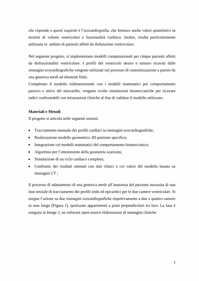
Il processo di adattamento di una generica mesh all’anatomia del paziente necessita di una
fase iniziale di tracciamento dei profili endo ed epicardici per le due camere ventricolari. Si
esegue l’azione su due immagini ecocardiografiche rispettivamente a due e quattro camere
in asse lungo [Figura 1], ipotizzate appartenenti a piani perpendicolari tra loro. La fase è
eseguita in Image J, un software open-source elaborazioni di immagini cliniche.

2
Figura 1 Immagini ecocardiografiche utilizzate, rispettivamente a 2 (sx) a e 4 (dx) camere in asse lungo.
I profili vengono poi importati in Blender, e disposti perpendicolarmente dall’operatore al
fine di viene ricreare la tridimensionalità considerando la relativa posizione delle finestre
di acquisizione delle immagini [Figura 2].
Nello stessa finestra di lavoro, un generico modello di una mesh biventricolare costruito
con elementi bidimensionali lineari viene ridimensionato in base ai profili tracciati.
Figura 2 Posizionamento dei profili in Blender (sx) per ricostruire la tridimensionalità sulla base
dell’orientamento del fascio durante la registrazione delle immagini (dx).
Conseguentemente in Continuity viene eseguito un fitting automatico che permette la
minimizzazione della distanza tra i contorni della mesh e i profili provenienti dalle
immagini cliniche.

3
In Continuity, software di maggior utilizzo in questo progetto, gli elementi della mesh
vengono suddivisi e resi tridimensionali passando da basi lineari lagrangiane a cubiche
hermitiane. La mesh così ottenuta presenta 129 elementi cubici e 209 nodi [Figura 3].
Figura 3 Esempio di mesh tridimensionale con basi hermitiane con 128 elementi cubici e 209 nodi.
Per il completamento del modello cardiaco, al modello geometrico vengono aggiunti i
modelli costitutivi per la caratterizzazione del tessuto biologico. In particolare viene
utilizzato il modello costitutivo proposto da Ogden-Holzapfel [5] con l’aggiunta di un
termine della “strain energy function” in funzione della comprimibilità del materiale. La
contrazione ventricolare si basa sul modello di Arts, nel quale la relazione forza-velocità
richiama il modello di Hill [6]. Le condizioni di pressione al contorno vengono specificate
dalla modellizzazione del sistema cardiopolmonare tramite i parametri derivanti dal
modello CircAdapt [7].
Il modello paziente-specifico è considerato completo con l’ulteriore inclusione
dell’architettura delle fibre cardiache, regioni di infarto del miocardio (se presenti) e
distribuzione dei tempi di contrazione durante la fase sistolica. Mentre il secondo ed il
terzo degli aspetti elencati sono caratteristiche paziente-specifico, questo studio prende in
considerazione una distribuzione delle fibre cardiache proveniente da un cuore umano ex-
vivo tramite la tecnica DT_MRI, assumendo valida l’ipotesi di conservazione
dell’orientamento delle fibre tra gli individui. La presenza di zone infartuate si riflette sui
parametri caratterizzanti sia il modello attivo che passivo.

4
La mesh così ottenuta si riferisce allo stato di fine diastole e al fine di calcolare
correttamente gli sforzi durante il ciclo cardiaco, è necessaria una configurazione a sforzo
nullo. A tal scopo viene adottato l’algoritmo proposto da Krishnamurthy [8] che richiede
come dati iniziali la mesh derivante dal processo di fitting e la pressione di fine diastole.
L’algoritmo prevede il raggiungimento di una geometria scaricata che, sottoposta ad una
fase di riempimento passivo, si deformi in nuova configurazione di fine diastole,
confrontata con quella di partenza per testare l’applicabilità del metodo.
In letteratura sono stati usati metodi matematici per stimare il volume scaricato. Questo
progetto prende come riferimento l’andamento della curva passiva introdotto da Klotz e
Co. [9] per un confronto coi valori simulati.
I modelli vengono poi utilizzati per la simulazione dell’intero ciclo cardiaco in modo tale
da studiare la capacità del modello derivante da immagini “Echo” di simulare il
comportamento in vivo paziente-specifico. Per la validazione dei risultati ottenuti si fa
riferimento sia ai dati clinici che ai modelli degli stessi pazienti sviluppati in precedenza da
altri autori [8] a partire da immagini CT.
Risultati
Il paragone tra modello Echo e CT viene in primo luogo effettuato analizzando
l’affidabilità dei volumi ventricolari delle mesh rispetto ai valori clinici derivanti dalle due
tecniche di immagine.
I volumi ventricolari dei modelli tridimensionali rispecchiano i volumi derivanti dalle
immagini cliniche. Si nota nei pazienti #2 e #3 analizzati che il volume ricavato dalle
immagini ecocardiografiche si discosta da quello valutato tramite la tecnica CT del 7.5% e
del 16% rispettivamente. Questo mette in luce alcune limitazioni dell’ecocardiografia: il
difficile rilevamento dei profili endo ed epicardici dovuto alla bassa qualità dell’immagine
e le assunzioni geometriche su cui si basano le formule volumetriche possono portare ad
una non accurata valutazione dei volumi ventricolari confronto lo standard di riferimento
(CT). Viene sottolineata la sovrastima delle pareti cardiache del modello tridimensionale
da parte dei modelli Echo rispetto a quelli CT. Questo limite è da rintracciare nella
modalità di fitting. Infatti, la mesh Echo viene interpolata ai profili ecocardiografici in soli
4 punti, appartenenti a due piani perpendicolari. Nel modello CT, la segmentazione delle

5
immagini permette di ottenere profili 3D che rendono più omogeneo e calibrato il
procedimento di fitting.
La discrepanza iniziale in termini di volume viene riflessa anche nella configurazione
scaricata, ed entrambi i metodi presentano un errore tra la geometria scaricata stimata e
quella calcolata col metodo di Klotz nella stessa percentuale, con una media dell’11%.
Si ritiene accettabile un errore tra la geometria ottenuta dal riempimento passivo della
geometria scaricata e il dato clinico di fine diastole paragonabile a quello tra la mesh di
post-fitting e il dato stesso.
La simulazione del ciclo cardiaco inizia dalla fase di contrazione isovolumetrica a partire
dalla nuova geometria insufflata. I valori di pressione durante il ciclo cardiaco simulati e
registrati in vivo presentano una differenza di circa il 5% per i modelli echo a confronto
dell’11% dei modelli CT [Figura 4]. Questo miglioramento è stato raggiunto agendo sul
parametro (σact ) del modello attivo al fine di far combaciare i risultati coi dati clinici. In
termini di frazione di eiezione, entrambi i modelli si discostano dal valore valutato
dall’esame ecocardiografico con un errore medio del 26.5%. Si ritiene necessario
sottolineare l’incertezza del dato clinico in termini di volumi. Essendo una tecnica
fortemente dipendente dall’ operatore, il valore ottenuto può essere alterato da quello reale.
Ulteriori risultati in termini di distribuzione del lavoro cardiaco sulla mesh derivante dalle
immagini Echo confermano la consistenza dei dati. La variabilità del lavoro cardiaco
ottenuto infatti caratterizza questa tipologia di pazienti affetti da un ritardo nella
contrazione del ventricolo sinistro. Come anche discusso in letteratura [10], generalmente
le aree che sviluppano maggior lavoro cardiaco sono situate alla base del ventricolo
sinistro.

6
Figura 4 Simulazione del ciclo cardiaco. Si riportano i cicli PV del ventricolo sinistro provenienti dal modello Echo
e CT (alto, sx) e l’andamento della pressione durante un ciclo comparata anche al dato clinico (basso dx).
Conclusioni
Lo scopo del presente studio è la realizzazione di modelli cardiaci 3D paziente specifico a
partire da semplici immagini ecocardiografiche 2D per pazienti affetti da disfunzione
ventricolare. Durante lo sviluppo del progetto, sono stati riconosciuti alcuni limiti:
In primo luogo l’utilizzo di sole due immagini ecocardiografiche 2D ha portato ad una
perdita di dettagli anatomici nel modello tridimensionale;
Il processo di fitting presenta degli ostacoli che richiedono una certa abilità da parte
dell’utente. A questo proposito sarebbe utile implementare un algoritmo automatico
che minimizzi la perdita di informazioni cliniche a partire dalla segmentazione delle
immagini;
I modelli matematici utilizzati si basano su numerosi parametri specifici quantificabili
tramite esami clinici invasivi: questo si contrappone all’esigenza di semplificazione
della costruzione del modello, oltre che aggravare lo stress sul paziente.
Si fa uso di un gruppo di proprietà passive mediate da quelle ricavate dagli autori del
modello CT. Questo potrebbe aver causato discostamenti e incongruenze nella
7
simulazione del ciclo cardiaco. Questo limite potrebbe essere superato utilizzando gli
stessi valori originali e confrontando nuovamente i risultati con modello CT.
Si sarebbe in grado di sopperire alla perdita di dettagli anatomici con l’impiego di un
numero più consistente di immagini 2D o con la tecnologia di ecografia 3D, che risulta
essere più in linea con il gold standard utilizzato.
Nonostante il percorso per raffinare il procedimento descritto e per diffondere l’utilizzo su
larga scala richiede numerosi miglioramenti, i risultati ottenuti costituiscono promettenti
basi per lo sviluppo di modelli cardiaci a partire da tecniche di immagine semplificate e di
costo contenuto.
Bibliografia
1. M. Neal, R. Kerckhoffs “Current progress in patient-specific modeling” 2009;
2. John Gorcsan III, Theodore Abraham, Deborah A. Agler, Jeroen J. Bax
“Echocardiography for Cardiac Resynchronization Therapy: Recommendations for
Performance and Reporting–A Report from the American Society of
Echocardiography Dyssynchrony Writing Group Endorsed by the Heart Rhythm
Society” 2008;
3. C. Sprouse, A. Jorstad, D. DeMenthon, P. Burlina, F. Contijoch, “Computational
Cardiac Modeling Based on Transesophageal Echocardiographic Imaging” 2010;
4. D. Deng, P. Jiao, X. Ye, and L. Xia “An Image-Based Model of the Whole Human
Heart with Detailed Anatomical Structure and Fiber Orientation” 2012;
5. Gerhard a. Holzapfel, R. W. Ogden “Constitutive modelling of passive
myocardium: a structurally based framework for material characterization” 2009;
6. J. Lumens,t. Delhaas, b. Kirn, t. Arts “Three-Wall Segment (TriSeg) Model
Describing Mechanics and Hemodynamics of Ventricular Interaction” 2009;
7. T. Arts, T. Delhaas, P. Bovendeerd, X. Verbeek, F. W. Prinzen “Adaptation to
mechanical load determines shape and properties of heart and circulation: the
CircAdapt model” 2004;
8. Adarsh Krishnamurthy, Christopher T. Villongco, Joyce Chuang , Andrew
McCulloch “Patient-specific models of cardiac biomechanics” 2012;

8
9. S. Klotz, I. Hay, M. L. Dickstein “Single-beat estimation of end-diastolic pressure-
volume relationship: a novel method with potential for noninvasive application”
2005;
10. Marieke Pluijmert, J. Lumens, M. Potse, T. Delhaas, Angelo Auricchio and Frits W
Prinzen “Computer Modelling for Better Diagnosis and Therapy of Patients by
Cardiac Resynchronisation Therapy” 2015;
Summary
With the continuous advances in computational processing speed, as well as modeling and
simulation methods, computer models of human physiology are starting to become viable
clinical tools to be used to improve diagnoses, aid in treatment planning and predict
therapeutic outcomes [1]. In particular for cardiac modeling, one of the main field of
interest regards the heart failure due to left ventricular (LV) systolic dysfunction with an
additional ventricular dyssynchrony. These patients are treated by Cardiac
Resynchronization Therapy, which resynchronizes the abnormal contraction sequences in a
manner that increases pumping effectiveness without increasing heart rate or myocardial
oxygen consumption [2]. The main issue related is that the 25%-35% of patients
undergoing CRT do not respond favorably. In this field, cardiac modeling is moving
forward to provide a quantifiable tool to understand a priori the responsiveness to the
treatment.
Cardiac computational models started fifty years ago and at the beginning they were only
used for very simple computational simulations of cardiac electrophysiology (EP) or
cardiac mechanics analysis. Due to the intensive research in this field and the evolution of
computing resources, the introduction of 3D advanced computational simulations of
cardiac EP and/or mechanics and model-based cardiac image analysis in clinical
environments are becoming more feasible [3].
Nowadays Computed Tomography is considered the gold standard procedure to obtain an
accurate geometry with a high level of anatomical details [4]. The main issue is the cost-
factor related to CT that limits the application of the cardiac model on clinical routine. On
the other hand, Ultrasound imaging is one of the most low-cost, safest, non-invasive
9
technique that is ideally suited for the evaluation of cardiac mechanics because of its
intrinsically dynamic nature. Furthermore, it plays an evolving and important role in the
care of heart failure patients treated with cardiac resynchronization therapy (CRT).
Therefore this study investigates the feasibility of using echocardiography as a basis for the
development of patient specific cardiac models and their application to the analysis of the
cardiac mechanics in patient affected by ventricular dysfunction.
Materials and Methods
The implementation of patient specific cardiac models is summarized with the following
subgoals:
Manual detection of endo and epicardial profiles from echocardiographic images;
Patient specific mesh creation;
Characterization of the mechanical properties through mathematical laws;
Unloaded Geometry Estimation;
Full-Beat Simulation: Hemodynamic and Local Work Analysis;
Comparison between Echo model results and clinical data and CT model.
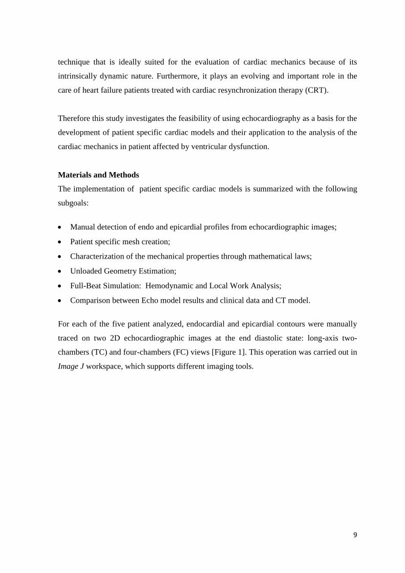
For each of the five patient analyzed, endocardial and epicardial contours were manually
traced on two 2D echocardiographic images at the end diastolic state: long-axis two-
chambers (TC) and four-chambers (FC) views [Figure 1]. This operation was carried out in
Image J workspace, which supports different imaging tools.
10
Figure 1 Echocardiographic images considered for profile detection: two chamber (left) and four chambers
(right).
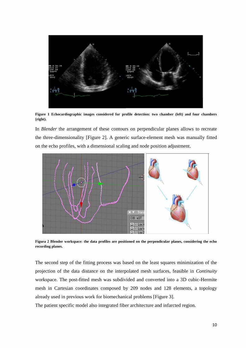
In Blender the arrangement of these contours on perpendicular planes allows to recreate
the three-dimensionality [Figure 2]. A generic surface-element mesh was manually fitted
on the echo profiles, with a dimensional scaling and node position adjustment.
Figura 2 Blender workspace: the data profiles are positioned on the perpendicular planes, considering the echo
recording planes.
The second step of the fitting process was based on the least squares minimization of the
projection of the data distance on the interpolated mesh surfaces, feasible in Continuity
workspace. The post-fitted mesh was subdivided and converted into a 3D cubic-Hermite
mesh in Cartesian coordinates composed by 209 nodes and 128 elements, a topology
already used in previous work for biomechanical problems [Figure 3].
The patient specific model also integrated fiber architecture and infarcted region.

11
Figure 3 Topology of 3D cubic-Hermite mesh used for cardiac modeling.
The myocardium was modeled as a non-linear slightly compressible material, with
anisotropic behavior ruled by the fiber structure. Mathematical models involved in this
project include myocardial passive and active mechanics. The first was based on Ogden-
Holzapfel [5] strain energy function, the latter on Art’s model, which includes a Hill type
force-velocity relation [6]. Kinematics constrains on the finite element mesh lead to avoid
undesired rigid body displacements and to simulate atria bounds.
The boundaries conditions in terms of intraventricular pressures were coupled to the
inward/outward blood flow, and hence to the time-dependent intraventricular volumes, by
means of a lumped-parameter model of the circulation, namely the CircAdapt circulatory
model [7].
In order to estimate an unloaded stress-free configuration, we adopted Krishnamurthy’s
algorithm [8], which makes use of the post-fitting end-diastolic mesh and end diastolic
pressure clinical value. The new loaded mesh obtained from the estimated unloaded
through passive inflation was compared to the post fitting mesh and the clinical data. The
estimated unloaded volume is compared to Klotz empirical volume together with CT
model unloaded volumes [9].
This new loaded mesh is the input for the full beat simulation, which starts with the
isovolumetric contraction. Hemodynamics information were elaborated in Matlab and
used for comparison with CT model results and clinical data in Results section.

12
Results
The reliability of Echo models was firstly confirmed by the end-diastolic fitted mesh
volume analysis. This showed a good agreement between clinical volume data and mesh
volume, meaning that the fitting process didn’t lead to significant loss in cardiac
ventricular dimension.
For patient #2 and #3 the volume estimated from echo images exceeded the volume from
CT by 7.5% and 16% respectively. This underlines some limitations of Echocardiography;
the detection of the myocardial contours complicated by the low image quality and the
geometric assumption at the base of volume formula may lead to an inaccurate volume
estimation compared to the one calculated by the gold standard CT. This difference was
also maintained in the unloaded configuration, which ratio with the fitted mesh was
constant between Echo and CT models for almost all cases.
The cardiac beat simulations were useful to underline that computational methods were
consistent with clinical data. In some cases Echo models matched the clinical data more
accurately than CT models. For example, the systolic peak was reached by the echo models
within the 5% of error compared to the 11% of CT models. The LV dP/dt index (velocity
of contraction) simulated by the Echo and CT models showed an averaged error of 6.5%
and 19% respectively compared to the clinical data.
Figure 4 Example of Cardiac PV loop plot (upper panel) and pressure time curve (lower panel): comparison
between Echo and CT model with clinical data.

13
Work distribution analysis underlines positively the ability of the echo model to simulate
the pathological altered mechanic function, showing good agreement with study in
literature [10].
Conclusions
The implementation of patient specific models of cardiac mechanics aimed to investigate
the Echocardiography as a potential low-cost tool for computational modeling in particular
for ventricular dysfunction pathology.
During the project development, the following limitations have been identified:
We noticed that the number of echo images used were not enough to accurately model
the anatomical detail;
Mesh segmentation and fitting steps: the employed method strongly depends on user
manual skill and should be improved to easily process images on large-scale databases.
Patient specific values: the mathematical models require a robust amount of patient
specific parameters, whose definition is based on invasive clinical exams. This aspect
enters in contrast with the project’s aim to use low-cost techniques.
Using an averaged group of material properties probably affected the full beat results
compared to CT model results. The next step could use the original patient-specific
properties in order to investigate if this improves the results.
The realization of a more accurate geometry with a lower loss of anatomical details could
be realized with the use of more than two imaging planes or even with the use of 3D echo
imaging.
The echo profile tracing step might be speeded up by implementing an algorithm for
automatic detection, making it less user-dependent. From a biomechanical point of view,
patient specific parameters should be derived where possible from non-invasive clinical
measurements in order to simplify the cardiovascular model and to relieve patient’s
burden.
Even if this research field still has to be improved in many aspects, this project shows
promising outcomes that lead to believe in a future application of echocardiography as the
low-cost clinical-routine tool to supply the required geometric data for cardiac mesh
construction.

14
References
1. M. Neal, R. Kerckhoffs “Current progress in patient-specific modeling” 2009;
2. Nelson GS, Berger RD, Fetics BJ, et al. “Left ventricular or biventricular pacing
improves cardiac function at diminished energy cost in patients with dilated
cardiomyopathy and left bundle-branch block” 2000;
3. C. Sprouse, A. Jorstad, D. DeMenthon, P. Burlina, F. Contijoch, “Computational
Cardiac Modeling Based on Transesophageal Echocardiographic Imaging” 2010;
4. D. Deng, P. Jiao, X. Ye, and L. Xia “An Image-Based Model of the Whole Human
Heart with Detailed Anatomical Structure and Fiber Orientation” 2012;
5. Gerhard a. Holzapfel, R. W. Ogden “Constitutive modelling of passive myocardium: a
structurally based framework for material characterization” 2009;
6. J. Lumens,t. Delhaas, b. Kirn, t. Arts “Three-Wall Segment (TriSeg) Model Describing
Mechanics and Hemodynamics of Ventricular Interaction” 2009;
7. T. Arts, T. Delhaas, P. Bovendeerd, X. Verbeek, F. W. Prinzen “Adaptation to
mechanical load determines shape and properties of heart and circulation: the
CircAdapt model” 2004;
8. Adarsh Krishnamurthy, Christopher T. Villongco, Joyce Chuang , Andrew McCulloch
“Patient-specific models of cardiac biomechanics” 2012;
9. S. Klotz, I. Hay, M. L. Dickstein “Single-beat estimation of end-diastolic pressure-
volume relationship: a novel method with potential for noninvasive application” 2005;
10. Marieke Pluijmert, J. Lumens, M. Potse, T. Delhaas, Angelo Auricchio and Frits W
Prinzen “Computer Modelling for Better Diagnosis and Therapy of Patients by
Cardiac Resynchronisation Therapy” 2015;

15
1. INTRODUCTION

16
Patient-specific modeling (PSM) is the development of computational models of human
pathophysiology that are individualized to patient-specific data. PSM is gaining more
attention from research groups around the world because of its potential to improve
diagnosis as additional modality, optimize clinical treatment by predicting outcomes of
therapies and surgical interventions, and inform the design of surgical training platforms
[1].
Cardiovascular disease (CVD) has been reported as the number one cause of death in the
world. It is estimated that by 2030, about 23.6 million people will die from a type of CVD.
It is a problem that crosses both gender and ethnicity and is a problem that gets worse with
age. Heart failure is usually the end result of most cardiac diseases. Therefore, correct
diagnosis and early prevention of CVDs are significantly important [2].
Mechanistic description, quantitative analysis, identification of causal interrelations,
consideration of dynamic behavior, and in particular prediction, are domains where
computational modelling has started to play a prominent role in cardiac research.
Cardiac computational models started fifty years ago and at the beginning they were only
used for very simple computational simulations of cardiac electrophysiology (EP) or
cardiac mechanics analysis [3].
Nowadays, 3D cardiac models are becoming increasingly complex and are currently used
in other areas such as cardiac image segmentation, statistical modelling of cardiac
anatomy, patient risk stratification or surgical planning. Since most cardiac reconstructive
operations (e.g., valve repair) are performed on a flaccid, empty heart under
cardiopulmonary bypass, the challenge for cardiac surgeons regards the accurate prediction
of how surgical modifications will behave under physiologic conditions [4].
Due to the intensive research in this field and the evolution of computing resources, the
introduction of 3D advanced computational simulations of cardiac EP and/or mechanics
and model-based cardiac image analysis in clinical environments are becoming more
feasible [3].
Current models incorporate multi-physics phenomena (Hunter et al., 2003; Kohl and
Noble, 2009, Nordsletten et al., 2011), combining electrophysiology (Trayanova, 2011),
mechanics (Nash and Hunter, 2000), mechano-electric interactions (Hermeling et al., 2012;
Hales et al., 2012), fluid flow (Taylor and Figueroa, 2009) and tissue perfusion (Lee and
Smith, 2012). They characterize processes across scales, from nano to macro. Cardiac
17
models increasingly incorporate subject-specific information, from ventricular anatomy to
electrical and mechanical material properties [5].
Finite element (FE) modelling, in combination with new cardiac imaging modalities and
advanced simulation tools, can be used to analyze mechanics of the pumping function of
the heart and mechanical properties of the myocardium . Such simulation models can
provide a greater insight of the pathophysiology thereby customizing the surgical planning
at best for that patient [6].
1.1. Cardiac Anatomy
The heart is a muscular organ about the size of a closed fist that functions as the body’s
circulatory pump. It takes in deoxygenated blood through the veins and delivers it to the
lungs for oxygenation before pumping it into the various arteries providing oxygen and
nutrients to body tissues by transporting the blood. The heart is located in the thoracic
cavity medial to the lungs and posterior to the sternum.
The base of the heart is located along the body’s midline with the apex pointing toward the
left side. Because the heart points to the left, about 2/3 of the heart’s mass is found on the
left side of the body and the other 1/3 is on the right.
The heart is a cave organ in which four chambers can be identified: the right atrium, left
atrium, right ventricle, and left ventricle. The atria act as receiving chambers for blood, so
they are connected to the veins that carry blood to the heart. The ventricles are the larger,
stronger pumping chambers that send blood out of the heart. The chambers on the right
side of the heart are smaller and have less myocardium in their wall thickness when
compared to the left side of the heart. This difference in size between the sides of the heart
is related to their functions and the size of the two circulatory loops. The right side of the
heart maintains pulmonary circulation to the nearby lungs while the left side of the heart
pumps blood all the way to the extremities of the body in the systemic circulatory loop.
To prevent blood from flowing backwards or “regurgitating” back into the heart, a system
of one-way valves are present in the heart. The atrioventricular (AV) valves are between
the atria and ventricles and only allow blood to flow from the atria into the ventricles. The
tricuspid valve (right side) and the mitral valve (left) are attached on the ventricular side to
tough strings called chordae tendineae. These pull on the AV valves to keep them from
folding backwards and allowing blood to regurgitate past them [Figure 1].

18
Figure 1.1 Anatomy of the heart longitudinal section: the deoxygenated blood flows in right atrium through vena
cava. During diastole, the blood is pushed in the right ventricle and then reached the lung during systole.
Contemporary, left ventricle receives oxygenated blood from left atrium, and pumps it to the rest of the body.
The heart wall is made of the three following layers:
Epicardium is the outermost layer of the heart wall and is a thin layer of serous membrane
that helps to lubricate and protect the outside of the heart.
Myocardium is the muscular middle layer of the heart wall that contains the cardiac
muscle tissue. Myocardium makes up the majority of the thickness and mass of the heart
wall and is the part of the heart responsible for pumping blood.
Endocardium is the simple squamous endothelium layer that lines the inside of the heart.
It is very smooth and is responsible for keeping blood from sticking to the inside of the
heart and forming potentially deadly blood clots.
The entire heart sits within in a serous membrane called pericardium which lubricates the
heart and prevents friction between the ever beating heart and its surrounding organs.
The cardiac ventricles have a complex three-dimensional muscle fiber architecture [7].
Although the myocytes are relatively short, they are connected such that at any point in the
normal heart wall there is a clear predominant fiber axis that is approximately tangent with
the wall (within 3 to 5◦ in most regions, except near the apex and papillary muscle
insertions).
Current methods for measuring fiber orientation range from histology to diffusion tensor
magnetic resonance imaging. It is known that fiber angle varies in a nearly linear fashion,
19
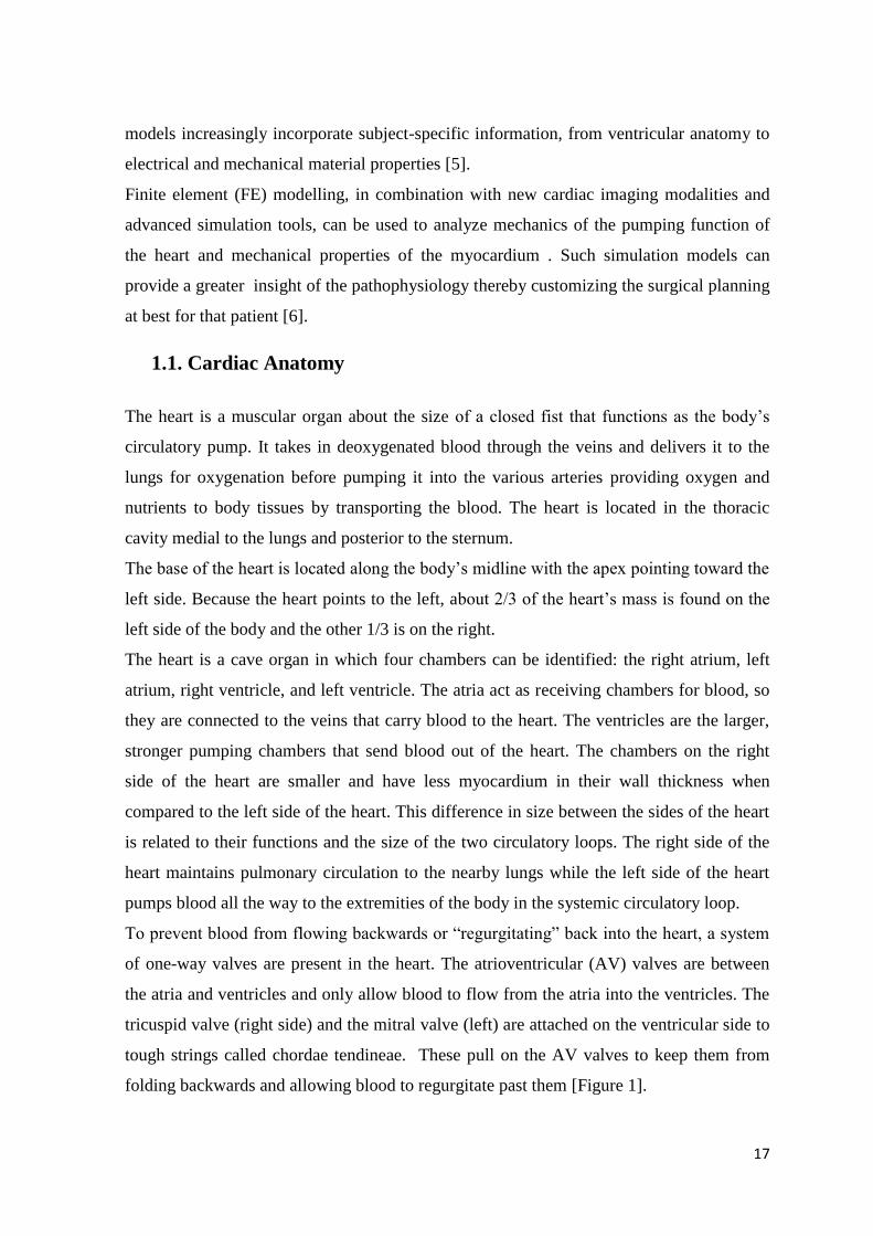
with a smooth transmural transition from the epicardium to the endocardium [8]. As can be
seen in the equatorial region, the predominant muscle fibre direction rotates from +50◦ to
+70◦ (sub-epicardial region) to nearly 0◦ in the mid-wall region to −50◦ to −70◦ (sub-
endocardial region) with respect to the circumferential direction of the left ventricle [9]
[Figure 1.2].
In the sinoatrial (SA) node, the heart has a natural pacemaker cells whose activation sends
the electrical signal to all the cardiac tissue in order to provide the contraction. The signal
from the SA node is picked up by another mass of conductive tissue known as the
atrioventricular (AV) node, located in the right atrium in the inferior portion of the
interatrial septum.
The AV bundle is a strand of conductive tissue that runs through the interatrial septum and
into the interventricular septum. The AV bundle splits into left and right branches in the
interventricular septum and continues running through the septum until they reach the apex
of the heart. Branching off from the left and right bundle branches are many Purkinje fibers
that carry the signal to the walls of the ventricles, stimulating the cardiac muscle cells to
contract in a coordinated manner to efficiently pump blood out of the heart [Figure 1.3].
Figure 1.2 Schematic diagram of: (a) the left ventricle and a cutout from the equator; (b) the structure through
the thickness from the epicardium to the endocardium; (c) five longitudinal–circumferential sections at regular
intervals from 10 to 90 per cent of the wall thickness from the epicardium showing the transmural variation of
layer orientation [9].

20
Figure 1.3 Cardiac conduction system: the electrical impulse starts in the Sinus Node (right atrium), runs to the
AV node and then is split into two branches in order to provide ventricles excitation.
The cardiac cycle includes three phases: atrial systole, ventricular systole, and relaxation.
Atrial systole: During the atrial systole phase of the cardiac cycle, the atria contract and
push blood into the ventricles. To facilitate this filling, the AV valves stay open and the
semilunar valves stay closed to keep arterial blood from re-entering the heart. The
ventricles remain in diastole during this phase.
Ventricular systole: During ventricular systole, the ventricles contract to push blood into
the aorta and pulmonary trunk. The pressure of the ventricles forces the semilunar valves
to open and the AV valves to close. This arrangement of valves allows for blood flow from
the ventricles into the arteries. The cardiac muscles of the atria repolarize and enter the
state of diastole during this phase.
Relaxation phase: During the relaxation phase, all 4 chambers of the heart are in diastole
as blood pours into the heart from the veins. The ventricles fill to about 75% capacity
during this phase and will be completely filled only after the atria enter systole. The
cardiac muscle cells of the ventricles repolarize during this phase to prepare for the next
round of depolarization and contraction. During this phase, the AV valves open to allow
blood to flow freely into the ventricles while the semilunar valves close to prevent the
regurgitation of blood from the great arteries into the ventricles.

21
1.2. Ventricular Dyssynchrony
The number of patients with chronic heart failure is increasing rapidly in the Western
world. Despite the introduction of new pharmacologic therapies, the prognosis of these
patients remains poor.
Ventricular dyssynchrony is a congestive heart failure (HF), associated with electrical and
conduction abnormalities. It consists in a delayed or altered pathways for ventricular
depolarization. There are two kinds defined: inter o intra ventricular dyssynchrony.
Interventricular dyssynchrony refers to the delayed activation of one ventricle with respect
to the other, whereas intraventricular dyssynchrony refers to the late activation of the
lateral regions of the left ventricular chamber as compared to the interventricular septum
[10].
Both of them are caused most of time by a heart disease or myocardial infarction which
brings an injury along the conduction system.
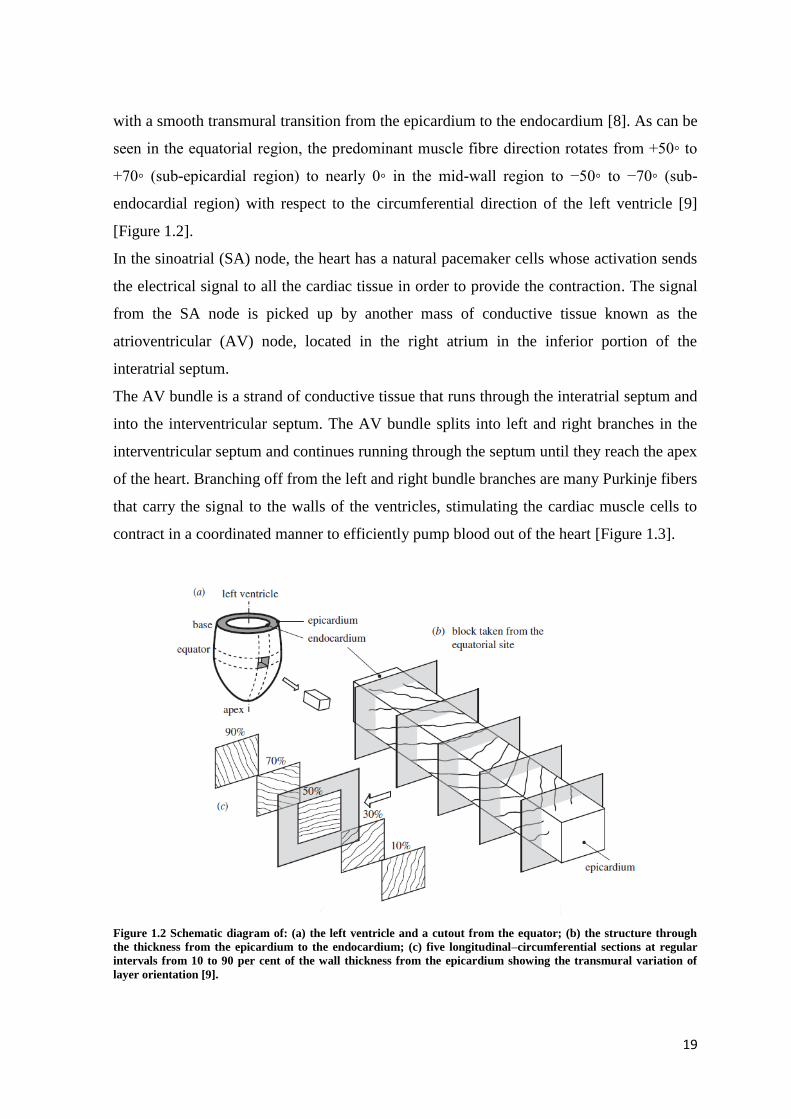
The electrical indicator for delayed asynchronous ventricular contraction in patients with
heart failure is most frequently a left bundle branch block (LBBB). Since the electrical
impulse can no longer use the preferred pathway across the bundle branch, it may move
instead through muscle fibers in a way that both slows the electrical movement and
changes the directional propagation of the impulses [Figure 1.4 A-B-C]. Electrical
dyssynchrony leads to mechanical dyssynchrony. As a result, there is a loss of ventricular
synchrony, ventricular depolarization is prolonged, and there may be a corresponding drop
in cardiac output .
In LBBB, the normal direction of septal depolarization is reversed (becomes right to left),
as the impulse spreads first to the RV via the right bundle branch and then to the LV via
the septum.
22
Figure 1.4 A) Physiological conduction system B) how the impulse spreads in a normal heart C) LBBB effect D)
Biventricular pacing implant (CRT) and electrical impulse restoration.
1.3. Cardiac Resynchronization Therapy
Despite promising pharmacologic treatments, chronic heart failure (CHF) remains a
leading cause of hospitalization and economic burden [12]. Heart transplantation and
implantable assist devices are possible for end-stage patients, though availability is limited
and costs are high.
Driven by these needs, a potentially simpler and more accessible treatment device has
emerged.
Cardiac resynchronization therapy (CRT) was introduced in the early 1990s, and
developed dramatically over time. Cardiac resynchronization therapy (CRT) also referred
to as biventricular pacing, is believed to resynchronize the abnormal contraction sequences

23
in a manner that increases pumping effectiveness without increasing heart rate or
myocardial oxygen consumption [11]. The clinical results are promising, and improvement
in symptoms, exercise capacity, and systolic left ventricular (LV) function have been
demonstrated after CRT, accompanied by a reduction in hospitalization and a superior
survival as compared with optimized medical therapy alone [10].
CRT improves the mechanical performance of the left ventricle and reduces mitral
regurgitation, resulting in relief of symptoms, improvement in exercise tolerance and
quality of life.
The prerequisite of resynchronization is achieved by placing a lead in the RV and another
in the left [Figure 1.4D]. Placement of RV lead is similar to standard pacemaker
implantation. The placement of the LV lead is most crucial. There is increasing evidence
that in patients with LBBB, the delayed electrical and mechanical activated region of the
LV is the posterolateral wall.
Pre-excitation of this region is therefore mandatory for achieving resynchronization within
the LV and between the two ventricles [12].
Not all patients with heart failure can be considered candidates for CRT and, with limited
experience to date, the indication for CRT is restricted to a group of patients who fulfill the
conditions and criteria used in the available trials. Currently approved recommendations
for CRT include patients with severe heart failure: New York Heart Association (NYHA)
functional class III or IV, widened QRS greater than or equal to 120 milliseconds, and LV
ejection fraction (EF) less than or equal to 35% [13].
Despite the great success of randomized clinical trials (MUSTIC [14] MIRACLE [15]),
approximately 25% to 35% of patients undergoing CRT do not respond favorably.
Because the vast majority of patients with wide QRS appear to have mechanical
dyssynchrony, an important goal of research groups is to improve patient selection for
CRT by identifying the subset of patients with wide QRS followed by mechanical
dyssynchrony. For this reason, the surface electrocardiogram may not be the optimal
marker to select candidates for CRT. The pathophysiologic reason for this scenario is
unclear, but it appears that patients with minimal to no dyssynchrony have a lower
probability of response to CRT and appear to have a poor prognosis after CRT [10].

24
1.4. Cardiac Imaging
Imaging has become an integral part of cardiac health and disease assessment. Several
cardiac imaging modalities are now widely available in the developed world, and are used
as part of standard procedures recommended by the relevant medical societies.
As models evolve towards clinical application, data from these imaging modalities are
commonly available to build personalized models. Understanding strengths and limitations
of the various techniques is fundamental for successful interrelation with computational
modelling [5].
Medical imaging modalities can roughly be categorized into two types based on their
energy sources: one is using ionizing electromagnetic radiation, such as conventional X-
ray and computed tomography (CT) using X rays and positron emission tomography
(PET), single-photon emission computed tomography (SPECT) using gamma rays; another
is using non-ionizing electromagnetic radiation, such as cMRI using radiofrequency and
cardiac echocardiogram using acoustic energy. Echocardiography, CT, MRI are currently
the most commonly used imaging modalities in clinical practice [2].
ECHO is a promising tool to understand assessment and benefits of CRT-patients, while
CT and MRI are a well confirmed imaging methods used for cardiac computational
models.
1.4.1. Echocardiography
Echocardiography has come a long way over the past 40-plus years. It is probably the
second most popular cardiac test, second only to the resting ECG. Echocardiographic
imaging is ideally suited for the evaluation of cardiac mechanics because of its intrinsically
dynamic nature [16].
A probe with gel on it is placed on the patient’s chest and generates a sound wave that
travels into the body. Part of the sound wave is reflected by different layers of the tissue
and returns to the probe which generates vibration. The vibration is translated into
electrical pulses into the ultrasonic scanner and processed into images [17].
There are four basic "modes" used to image the heart:
Two-dimensional (2D) imaging
M-mode imaging
25
Doppler imaging
Three-dimensional (3D) imaging
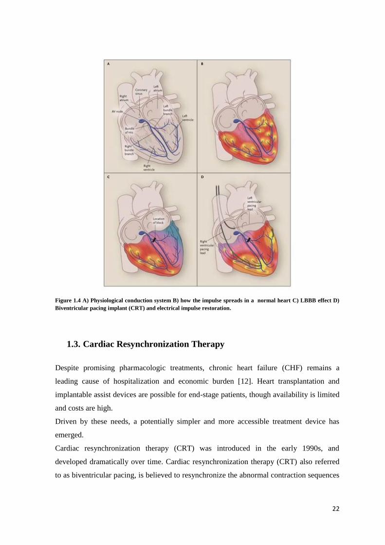
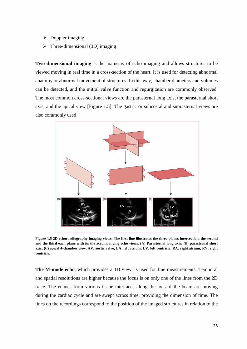
Two-dimensional imaging is the mainstay of echo imaging and allows structures to be
viewed moving in real time in a cross-section of the heart. It is used for detecting abnormal
anatomy or abnormal movement of structures. In this way, chamber diameters and volumes
can be detected, and the mitral valve function and regurgitation are commonly observed.
The most common cross-sectional views are the parasternal long axis, the parasternal short
axis, and the apical view [Figure 1.5]. The gastric or subcostal and suprasternal views are
also commonly used.
Figure 1.5 2D echocardiography imaging views. The first line illustrates the three planes intersection, the second
and the third each plane with its the accompanying echo views. (A) Parasternal long axis; (B) parasternal short
axis; (C) apical 4-chamber view. AV: aortic valve; LA: left atrium; LV: left ventricle; RA: right atrium; RV: right
ventricle.
The M-mode echo, which provides a 1D view, is used for fine measurements. Temporal
and spatial resolutions are higher because the focus is on only one of the lines from the 2D
trace. The echoes from various tissue interfaces along the axis of the beam are moving
during the cardiac cycle and are swept across time, providing the dimension of time. The
lines on the recordings correspond to the position of the imaged structures in relation to the
26
transducer and other cardiac structures at any instance in time. The M-mode
echocardiogram yields cleaner images of cardiac borders, allowing the operator to obtain
more accurate measurements of cardiac dimensions and more critically evaluate cardiac
motion.
Doppler imaging allows evaluation of blood flow patterns, direction, and velocity.
Doppler echocardiography is based on detection of frequency changes (the Doppler shift)
occurring as ultrasound waves reflect off individual blood cells moving either away from
or toward the transducer.
Three-dimensional imaging (3D Echo) has been recently developed and allows to obtain
a tridimensional view of the ventricular chambers. Compared to the 2D echocardiography,
whose volume calculation strongly depends on the analytical formulas choosen, the 3D
shows better results in terms of reliability and reproducibility [19].
With this instrumentation versatility, it is not surprising that the amount of clinical
information provided by a cardiac ultrasound examination has grown over the years. The
various examinations provide a highly detailed, real-time examination of cardiac anatomy
and function.
This ultrasonic tool has had an immense impact on understanding of a variety of disease
states, such as pericardial effusion, intracardiac masses, valvular, congenital and
myocardial disease. It is probably the most practical tool for judging regional left
ventricular dysfunction secondary to coronary artery disease [18].
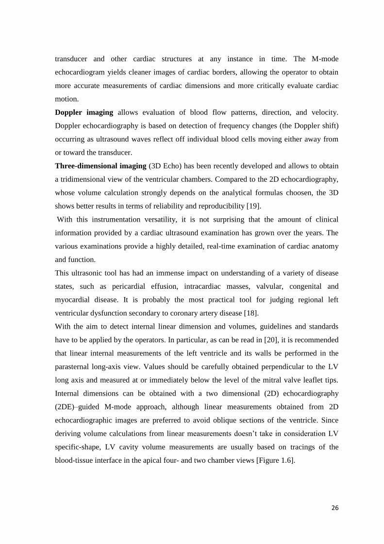
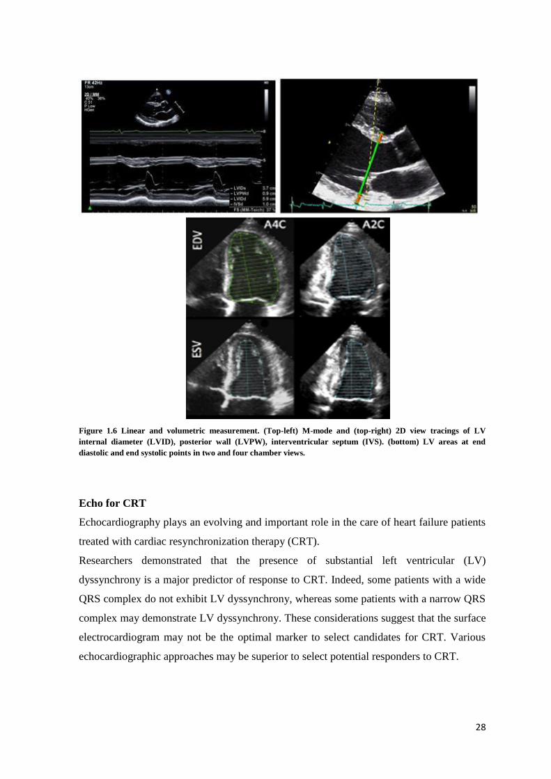
With the aim to detect internal linear dimension and volumes, guidelines and standards
have to be applied by the operators. In particular, as can be read in [20], it is recommended
that linear internal measurements of the left ventricle and its walls be performed in the
parasternal long-axis view. Values should be carefully obtained perpendicular to the LV
long axis and measured at or immediately below the level of the mitral valve leaflet tips.
Internal dimensions can be obtained with a two dimensional (2D) echocardiography
(2DE)–guided M-mode approach, although linear measurements obtained from 2D
echocardiographic images are preferred to avoid oblique sections of the ventricle. Since
deriving volume calculations from linear measurements doesn’t take in consideration LV
specific-shape, LV cavity volume measurements are usually based on tracings of the
blood-tissue interface in the apical four- and two chamber views [Figure 1.6].
27
More issues are present with the RV dimension tracings. Measurements by 2DE are
challenging because of the complex geometry of the right ventricle and the lack of specific
right-sided anatomic landmarks to be used as reference points.
3D Echocardiography allows measurements of RV volumes, thereby overcoming the
limitations of conventional 2DE RV views with respect to orientation and reference points.
As with all technologies, there are advantages and disadvantages. One of the reason why
this method is particularly preferred among the others is concerned with non-invasivity,
rapid evaluation, safety for the patient, availability in the operating theatre. It’s also a
ionising radiation free tool and the device requires an easy transportation to the bedside.
If performed properly and for the right reason, this test should be very cost effective and
should be a major asset in the coming era of medical cost containment [16].
The principal disadvantage is the fact that education and training are imperative to provide
high-quality examinations and proper interpretations; there might be errors in the results
due to the operator influence. In addition, many of the diagnoses are still qualitative and
subjective, sometimes images have low quality and resolution.
28
Figure 1.6 Linear and volumetric measurement. (Top-left) M-mode and (top-right) 2D view tracings of LV
internal diameter (LVID), posterior wall (LVPW), interventricular septum (IVS). (bottom) LV areas at end
diastolic and end systolic points in two and four chamber views.
Echo for CRT
Echocardiography plays an evolving and important role in the care of heart failure patients
treated with cardiac resynchronization therapy (CRT).
Researchers demonstrated that the presence of substantial left ventricular (LV)
dyssynchrony is a major predictor of response to CRT. Indeed, some patients with a wide
QRS complex do not exhibit LV dyssynchrony, whereas some patients with a narrow QRS
complex may demonstrate LV dyssynchrony. These considerations suggest that the surface
electrocardiogram may not be the optimal marker to select candidates for CRT. Various
echocardiographic approaches may be superior to select potential responders to CRT.

29
Numerous recent published reports have utilized echocardiographic techniques to
potentially aide in patient selection for CRT prior to implantation and to optimized device
settings afterwards [10].
For example, interventricular dyssynchrony can be evaluated by assessing the extent of
interventricular mechanical delay (IVMD), defined as the time difference between left and
right ventricular pre-ejection intervals [Figure 1.7]. An IVMD > 40ms is considered
indicative of interventricular dyssynchrony.
M-mode echocardiography may be useful for assessing intraventricular dyssynchrony.
Using an M-mode recording from the parasternal short-axis view (at the papillary muscle
level), the septal-to-posterior wall motion delay (SPWMD) can be obtained, and a cut-off
value >130 ms was proposed as a marker of intraventricular dyssynchrony [10].
Figure 1.7 Measurement of the interventricular mechanical delay (IVMD) by Doppler echocardiography: the
right ventricular and left ventricular (LV) preejection intervals are measured from the onset of the QRS on the
electrocardiogram (ECG) to the onset of pulmonary (Pulm) (RV-PEI) and aortic (Ao) (LV-PEI) outflow; IVMD is
calculated by subtracting the RV-PEI from the LV-PEI.
1.4.2. Computed Tomography
Computed Tomography (CT) provides excellent anatomical resolution, both spatial and
temporal, but it involves exposure to ionizing radiation.
This method utilizes tomography to create a 3D volume of transmission images using 2D
X-ray images. They are taken around a single rim of rotation where x-rays are delivered to
the body of interest in multiple directions. The different radio-densities of different tissue
types enable the generation of a large number of 2D x-ray images, revealing the interior of
the body. An imaging computer is used to reformat and reconstruct the 2D images and 3D
representation of the structures [2].
30
The CT scan’s diagnostic ability can make surgical biopsy or exploratory surgery
unnecessary. Its real-time imaging allows CT scanning to be used to guide needle biopsies
and similar procedures. A cardiologist can view clear 3D images of the coronary arteries
without having to do an invasive angiography.
The principal advantages of CT are rapid acquisition of image, a wealth of clear and
specific information, view of a large portion of the body.
1.4.3. Magnetic Resonance Imaging
Magnetic resonance imaging (MRI) is an imaging technique used primarily in medical
settings to produce high quality images of the inside of the human body. MRI is based on
the principles of nuclear magnetic resonance (NMR), a spectroscopic technique used by
scientists to obtain microscopic chemical and physical information about molecules.
Cardiac Magnetic Resonance Imaging (MRI) can provide a rich set of data, including
information on cardiac anatomy, mechanics, microstructure, perfusion, and other tissue
properties. Consequently, it is considered the gold-standard for assessing cardiac anatomy
and function [5].
One of the main advantages of cardiac MRI is the lack of ionizing radiation, which is
substantial computed tomography (CT) scanning. The strength of cardiac MRI, as
compared with CT scanning, is its superior temporal and contrast resolution. However, the
spatial resolution of CT scanning is superior.
The acquisition of images from CMR can be done in different sequences, and the
tomographic planes can be arranged in space according to different criteria.
Two main sequences are used: the first provides views on the short axis, in which the heart
is segmented with a series of planes perpendicular to the long axis ventricular and
uniformly distributed along it.
In these images is readily detectable the thickness of the ventricular wall and the volume of
the ventricle. However, since the distance between consecutive planes is typically several
millimeters, identifying the mitral valve is often not possible, neither the ventricular apex.
The second sequence provides long axis views, in other words on planes passing through
the ventricular long axis. In particular, the views are commonly so-called two-chamber (in
which are visible atrium and ventricle claims), three-room (in which are visible atrium and
ventricle and the aorta claims) and four rooms (in which are visible all four heart

31
chambers). Compared to the short axis view, in this case there’s visibility of the mitral
valve, ventricular apex and also the position of the papillary muscles. Joining together the
two axis views allows to have an exhaustive description of the geometry of the ventricle,
producing a 3-dimensional model of the area of interest being scanned [Figure 1.8].
Furthermore, the image acquisition can be done also on rotational planes, where once the
ventricular axis is set, the segmentation planes are those containing that axis and rotated
within a fixed angle.
Figure 1.8 Cardiac MRI image: A) short axis, B) long axis views.
1.5. Cardiac Imaging for cardiac computational models
The evolution of medical imaging technology gives the possibility of building realistic 3D
cardiac models from either in-vivo or ex-vivo images.
The uptake of echocardiographic data for computational model development has been
limited so far, but insightful case examples exist: e.g. its use in combination with simple
mechanical models to identify the contribution of the right ventricle to improved pump
function induced by cardiac resynchronization therapy (Lumens et al., 2013), or to evaluate
the relevance of different dyssynchrony indexes to predict the response to the same therapy
(Lumens et al., 2012).
CT has become an important imaging tool due to its accuracy and high spatial resolution.
The excellent anatomical detail provided by this imaging modality has enabled detailed
computational investigations, it provides the opportunity to build patient-specific

32
ventricular models of subjects with implantable devices, such as a left ventricular assisted
device.
Deng et al. built an anatomically detailed mathematical model of the human heart, firstly
reconstructed from the computed tomography images [21] [Figure 1.9].
Since MRI provides a rich set of data with the possibility of obtaining accurate anatomical
and functional information from a single imaging modality, a relatively “clean” appearance
of the images (in comparison to echocardiography), nowadays this technique has become
the gold-standard for cardiac modeling.
In general, computed tomography (CT) offers superior resolution and contrast than
Magnetic Resonance Imaging (MRI) , however the latter is more commonly used in
clinical cardiology and therefore as a basis for in vivo computational modelling [22].
Figure 1.9 Image processing of the construction of human heart model: from the original CT image (top left) to
frontal and back view of the reconstructed model (bottom middle and right).
1.6. Project’s overview and goal
Nowadays the trend of development of patient-specific (PS) cardiac models is increasing
exponentially in order to reach highly detailed description of anatomy and
electromechanical simulation of the organ.
This is growing in parallel with computational tools, becoming day-by-day more and more
sophisticated.
33
Looking at a future projection of PS models in clinical and daily routine, the complex and
labor-intensive process of generating models might be in contrast with surgery and
diagnostic world where relatively fast turnaround times are required. This consideration
leads to think a possible way clinicians might have to build a time-realistic PS anatomical
and mechanical model with fast, low-cost technique with the aim to study the best
customized treatment without wasting of time and resources.
This task must face the compromise between highly detailed-accurate-expensive modeling
on one side and a modeling based on easy method of calculation, low-cost, relative-fast,
non-invasive test on the other side.
This study stands at this projection of large scale performance of cardiac models and
chases the challenge to find the right substitute for CT and MRI imaging techniques to
make the modeling process easier to develop without loss of patient-specific feature.
In particular, this project focuses on using ECHO images as the source for anatomical 3D
geometry for patient affected by interventricular dyssynchrony. As showed above, there
are many issues in understanding a priori if the patient can benefit from CRT implantation
and Echocardiography is one of the first and most common test to which the patient has to
undergo in this field.
An echo image-based computational model uses data from a routine test, first used for
cardiac pathological patients for quantification and assessment of the disease, looking
forward for hospital resource savings.
In this contest, biventricular models of five patients affected by left ventricular dysfunction
with/without infarcted regions are analyzed and used for mechanical simulations which
includes unloaded geometry and cardiac full beat.
A comparison between Echo and CT image-based models is discussed, taking into account
previous study on the same patients, made available by Cardiac Mechanic Research Group
Lab from University of California San Diego.

34
2. STATE OF ART
35
2.1. General Approach to Human Heart Modeling
A biomechanical heart model typically includes modular aspects such as: i) a geometry
representing the heart in its anatomical features, ii) a constitutive model showing the
passive behavior of the tissue, iii) an active model for the active contraction during the
pumping phase of the heart cycle and iv) a hemodynamic-circulatory model.
The first developed 3D computational models of cardiac anatomy were simplistic models
based on geometric shapes. Due to the highly complex anatomical structure of the heart,
some radical simplifications have been considered helpful and actually necessary since
researchers started to be interested in representing the heart geometry.
The most important approximation consisted in the assumption of an axisymmetric
geometry for the left ventricle which was popular in early studies of the heart and was
helpful for a better basic understanding of the heart function. Thereby, some investigators
approximated the geometry of the left ventricle by a thin-walled cylinder, sphere or
ellipsoid [23,24]. Most of them only included the left ventricle (LV), represented by two
concentric ellipsoids truncated at the base level to roughly approximate the shape of the
LV [3]. This kind of geometry are still used nowadays when the anatomical feature is not
crucial for the aim of the project. Geometric models have been very useful in the analysis,
especially the use of confocal and non-confocal ellipsed of revolution to describe the
epicardial and endocardial surfaces of the left and right ventricular walls.
Later in time, next to the geometrical shape, there have been placed anatomical shapes for
the heart model constructed by manual drawing from histo-anatomical slices or from
measurements taken on explanted hearts or by segmenting pictures of histo-anatomical
slices [25,26]. The most representative ones are two bi-ventricular models highly
referenced and reused: the rabbit model from University of California San Diego [25] and
the canine model from University of Auckland [26]. The latter was reasonably modeled by
a thick ellipsoid of revolution truncated at the base.
These simplifications of the geometry were usually accompanied by other approximations
with respect to the material behavior. For example, in early attempts for the modelling of
the heart, assumptions like isotropy and linear elasticity of the material were widely used.
Depending on the assumptions about the geometry, the material behavior and the boundary
conditions, these models yielded sometimes quite different predictions of the
circumferential or longitudinal distribution of the wall stress in the myocardium [27,28].
36
Across the ‘70s, the physiological distribution of the myocardial fibers was confirmed by
experimental studies [29] and this lead to a more accurate description of the myocardium
representation and behavior. Besides this, analytic procedures were only possible with
extremely limiting assumptions both in terms of geometry and mechanical model.
More refined constitutive models and complicated geometries have to be treated
numerically. Thereby, the Finite Element (FE) method lends itself for this purpose, as it is
suited to treat irregular solid geometries, boundary conditions and nonlinear multiphase
constitutive properties [30].
During the last twenty years with the deep advance in medical imaging technologies, more
and more details about the heart from subcellular structure to whole organ have been
discovered. The increasing availability of in-vivo cardiac images together with the rising
trend towards personalized medicine yield researchers to base the model not only on a pre-
fixed geometric shape but they begin to use cardiac imaging (CT, MRI) as the source to
reproduce the patient-specific anatomy [3].
So far the synergy between experimental methods (e.g. data from images and functional
maps) and theory (computational models) has been seen as the key in the generation of
novel insight in cardiovascular science. Development of computational models relies on
information from images. Image data have become drivers of progress in cardiac
computational modelling in three general areas [Figure 2.1]. First, they capture anatomy,
providing the structural information necessary to run simulations.
Secondly, images provide functional information used to build, adjust and validate models.
Thirdly, images are used to estimate model parameters by data assimilation, finding the
model parameters that best explain the observed data [5].
The need to personalize the finite element mesh with the patient imaging data came also
from the challenge to improve medical care with the cardiac modeling. Above all
considering many cardiac pathologies, as dilate cardiomyopathy, the specific shape has to
be part of the model because highly affects the mechanical behavior and passive material
properties.
Furthermore, patient-specific models of cardiovascular mechanics can play an important
role in the development of medical devices.

37
2.2. Patient Specific Cardiac Anatomy Reconstruction
Methods for quantifying the anatomy for patient-specific modeling of cardiovascular
mechanics include noninvasive imaging techniques such as CT, MRI and ECHO.
The accuracy of the model reconstruction depends on the type of imaging technique used.
While MRI and CT are higher resolution and frequently used in research field, they are
expensive and exceptional for heart failure patients. On the other hand, Echocardiography
is routinely performed in HF (heart failure) patients to assess ventricular morphology and
measure quantitative hemodynamic and ventricular pump function [31].
In general the cardiac geometry is built either as a triangles-based surface if the fields of
interest are the ventricular cavity and the endocardium , or as a solid subdivided by
hexahedral or tetrahedral elements more suitable for myocardial wall studies.
One of the way to obtain the patient specific geometry is to fit a template on the image.
Krishnamurthy &Co. [32] manually segmented endocardial and epicardial contours (left
ventricle, right ventricle, septum and epicardium) of the patient heart from CT images. An
initial 2D Cubic-Hermite template mesh was pre-fitted by placing the nodes at the common
anatomical landmarks (left ventricular lateral wall, right ventricular lateral wall, base, apex
and the septum-right ventricular junctions) to preserve the structure of the mesh relative to
the patient heart. Later a second fitting in the radial coordinates was computed following
Nielsen et all [26] approach based on linear least square minimization of the projection
distance of the data to the interpolated mesh surfaces parameterized at the nodes. This
mathematical method uses a prolate spheroidal coordinate system because it provides a
good initial approximation to ventricular boundary geometry and permits the use of a
linear least-squares fitting algorithm in which only the radial coordinate is fitted [26].
Cardiac Images
Cardiac Models
Capture structure
and function
Are validated
against
Data
assimilation
Figure 2.1 Interconnection between Cardiac images and Models

38
A similar approach was used by Aguado-Serra&Co but starting from echo images [31].
Owing to the low resolution of ultrasounds images, the resulting geometric model can be
fitted using fewer degrees of freedom, although there is a corresponding loss of anatomic
detail. Using the least square finite element methods and initializing the prolate spheroidal
model with a small number of manually identified landmarks at the base and apex, the
biventricular mesh is fitted with 2D echocardiographic recordings of the patient [Figure
2.2].
Figure 2.2 Biventricular mesh fitted with 2D echocardiographic image.
Sermesant &Co segmented the myocardium from 3D image of the heart using classical
image processing methods like thresholding and mathematical morphology. They used the
marching cubes method in order to obtain the triangulated surface of the myocardium and
the volumetric tetrahedral mesh is created from the triangulated shell through specific
software [67] [Figure 2.3 Upper Panel].
Niederer and colleagues provided a myocardial reconstruction from MRI images. These
were manually segmented to identify three surfaces: epicardium, left ventricle and right
ventricle endocardium. Two dimensional bi-cubic Hermite finite elements were fit to each
of the three surfaces and successively the surface meshes were converted into tri-cubic
Hermite volume elements [Figure 2.3 Lower Panel] [68].
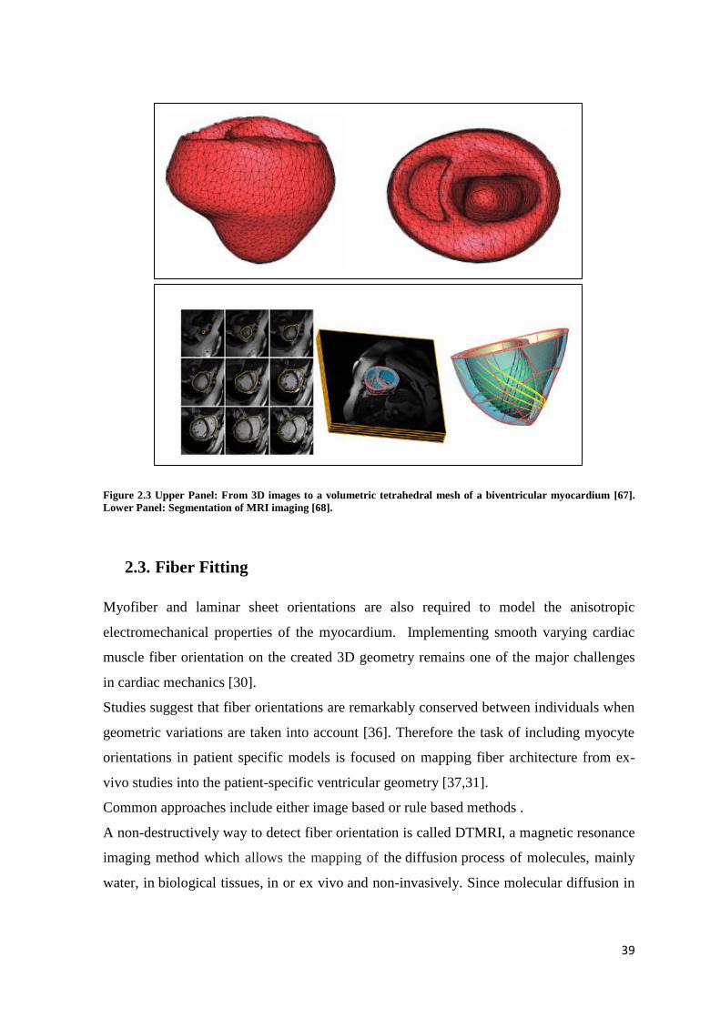
39
Figure 2.3 Upper Panel: From 3D images to a volumetric tetrahedral mesh of a biventricular myocardium [67].
Lower Panel: Segmentation of MRI imaging [68].
2.3. Fiber Fitting
Myofiber and laminar sheet orientations are also required to model the anisotropic
electromechanical properties of the myocardium. Implementing smooth varying cardiac
muscle fiber orientation on the created 3D geometry remains one of the major challenges
in cardiac mechanics [30].
Studies suggest that fiber orientations are remarkably conserved between individuals when
geometric variations are taken into account [36]. Therefore the task of including myocyte
orientations in patient specific models is focused on mapping fiber architecture from ex-
vivo studies into the patient-specific ventricular geometry [37,31].
Common approaches include either image based or rule based methods .
A non-destructively way to detect fiber orientation is called DTMRI, a magnetic resonance
imaging method which allows the mapping of the diffusion process of molecules, mainly
water, in biological tissues, in or ex vivo and non-invasively. Since molecular diffusion in

40
tissues reflects interactions with many obstacles, such fibers, the diffusion tensor (DT)
provides regional information on myofiber architecture throughout the ventricular wall. It
has been provided that the primary axis of water diffusion in myocardium is like to
coincides with the mean myofiber direction [59] .
In literature, the DTMRI information has been applied to the personalized anatomical
model with the help of mathematical rules, such as Log-Euclidean metric proposed by
Arsigny [38]. This method to transform from imaging to three dimension vector
components can preserve the major and minor axes of the diffusion tensor derived from
human hearts [31].
Besides this, Krishnamurthy and Co. make use of large deformation diffeomorphic
mapping in order to fit differences among patients such as ventricle size and shape, starting
from a DTMRI on a single donor heart [37].
Some other groups include the mapping of fiber orientation in the model through a rule-
based method. The main idea of the rule-based algorithm is to generate fiber direction on
the 3D geometry using mathematical descriptions which are derived from the histological
data.
Recently, few researchers used Laplace interpolation with Dirichlet boundary conditions to
implement fiber map on 3D geometry. As termed, implementation of this algorithm needs
boundary conditions which in this case is the LV and right ventricle (RV) endocardium and
epicardium surfaces. But automatic separation of the different surface domains is difficult
and thus prevents the algorithms to act automatically [39,40].
This algorithm has the potential to be used with the experimental data (DTMRI) to
interpolate in the region where data is not sufficient enough to draw the fiber directions
[41].
Bishop et al. [55] show that global electrical activation patterns obtained by computational
simulation from a model with fiber orientation based on a rule-based linear approach were
very similar to those based on DTI for the same geometry, thus demonstrating the
robustness of the former method for EP simulation studies [Figure 2.4].

41
Figure 2.4 Different methods to include the fiber orientation in 3D bi-ventricular models. Comparison between (a)
rule-based method (Laplace-Dirichlet) and (b) DTI-based estimation of the myocardial fiber orientation for a 3D
model of canine ventricles [39].
2.4. Constitutive model
Next to a realistic descriptions of the three-dimensional geometry and structure of the
myocardium, one task of central importance is the description of ventricular mechanics.
This is supported by continuum balance laws, boundary conditions and, most importantly,
constitutive equations that characterize the material properties of the myocardium together
with statistical parameter estimation and validation [9].
There are several models of the elasticity of the myocardium available in the literature,
including isotropic models (e.g. Demiray 1976), transversely isotropic models
(e.g. Humphrey&Yin1987;Humphrey et al. 1990; Guccione et al. 1991; Costa et al. 1996)
and orthotropic models (e.g. Hunteret al. 1997; Costa et al. 2001; Schmid et al. 2006).
One problem in developing an adequate constitutive model is the shortage of experimental
data suitable for detailed parameter estimation in specific functional forms. The orthotropic
nature of the myocardium has already been highlighted by different authors (Dokos 2002),
but very often this mechanical description is simplified due to the lack of set of data.
There are some aspects of this muscular biological tissue hardly taken in consideration in
computational modeling. For example, viscoelasticity is not important from the point of
view of mechanical modelling on the time scale of the cardiac cycle, which is short
compared with the relaxation time of the viscoelastic response. Instead residual stresses

42
have an important influence on the stress pattern in the typical physiological state but
three-dimensional ones are very difficult to quantify and hence their modelling must be
treated with caution [9].
In the present work, the myocardium has been considered transversely isotropic material
described by constitutive model developed by Holzapfel and Ogden [9] .
The strain energy function Ψ per unit reference volume is the mean to describe the material
properties and it is additively decomposed into volumetric Ψvol and isochoric part Ψiso.
𝜳 tot = 𝜳 vol(J) + 𝜳 iso(I1, I4) (1)
where Ψvol(J) and Ψiso(I1,I4) are given function of J and the isochoric invariants I1, I4
(see Appendix).
The slightly compressible Ψvol(J) volumetric energy component is defined as:
𝚿vol(J) = K(J − 1) ∗ ln(𝐽) /2 (2)
With K is the user-specified bulk-modulus and serves as a penalty parameter to incorporate
material incompressibility [56] .
The second expression of the strain energy function is defined by a separated exponential
terms in order to describe the anisotropy in the fiber and cross fiber directions.
The former (with scaling parameter a and exponent b) corresponds to the isotropic material
properties of the tissue, while the latter (with scaling parameter af and exponent bf)
corresponds to the fiber direction passive properties.
𝚿iso = 𝑎
2∗𝑏𝑒𝑏(𝐼1−3) +
𝑎𝑓
2∗𝑏𝑓(𝑒𝑏𝑓(𝐼4𝑓−1)^2 − 1) (3)
With
I1 : the first invariant of the right Cauchy-Green tensor
I4: components of the right Cauchy-Green strain tensor in fiber direction
a,b,af,bf : material properties
43
The anisotropic resting material parameters (a,b,af,bf) were estimated with data obtained
from Krishnamurthy’s paper “patient specific modeling of cardiac biomechanics” (see
Appendix for values).
The Cauchy stress is valuated through the derivative of 𝜳𝒕𝒐𝒕, with the following equation:
𝛔𝑝𝑎𝑠𝑠 =1
𝐽∗ 𝑭 ∗
𝑑𝚿𝐭𝐨𝐭
𝑑𝑭 (4)
2.5. Unloaded Geometry
The in-vivo cardiac images used for extracting the patient specific geometry usually refers
to the end diastolic point of the cardiac cycle.
However, an unloaded stress-free reference state is required to compute the stress and
strain correctly. This unloaded geometry, when loaded to the measured end-diastolic
pressure, deforms to the measured end-diastolic geometry previously obtained from
clinical images [42].
In literature, some studies have considered the end-systolic or mid-diastolic geometry as
the unloaded stress-free state for simplification. However, a recent study shows that the
effects of residual stresses are relatively small in diastole [43,44,45,6].
Klotz and Co [46] reported an empirical relation for the unloaded left-ventricular cavity
volume as a function of the end-diastolic pressure and cavity volume that was found to
correlate well with measurements in human and animals hearts.
Given Vm and Pm measured volume and pressure respectively, the unloaded volume (V0 at
0 mmHg) can be obtained from:
𝑉0 = 𝑉𝑚(0.6 − 0.006 ∗ 𝑃𝑚) (5)
The pressure-volume curve (EDPVR) can be predicted from analytical determination of
the set of parameters shown in the following equations:
𝐸𝐷𝑃 = α ∗ 𝐸𝐷𝑉𝑛𝛽 (6)
44
𝐸𝐷𝑉𝑛 =𝑉𝑚−𝑉0
𝑉30−𝑉0 (7)
𝑉30 = 𝑉0 +𝑉𝑚−𝑉0
(𝑃𝑚
α)
1𝛽
(8)
𝛽 =𝐿𝑜𝑔(
𝑃𝑚30⁄ )
𝐿𝑜𝑔(𝑉𝑚
𝑉30⁄ )
(9)
α =30
𝑉30𝛽 (10)
Where:
EDP = end diastolic pressure
EDVn = end diastolic volume normalized
Vm, Pm = input data, volume and pressure during the cardiac cycle
V30 = volume at 30mmHg
In this way choosing Vm and Pm at end-diastolic point, the unloaded volume can be
evaluated.
In this project, a computational method developed by Krishnamurthy to estimate the
unloaded geometry [32] [Figure 2.5].
The algorithm is based on an iterative estimation scheme that minimizes the difference
between the measured end diastolic geometry and the computed geometry when the
unloaded model is inflated to the measured end-diastolic pressure assuming a nonlinear
myocardial material properties.
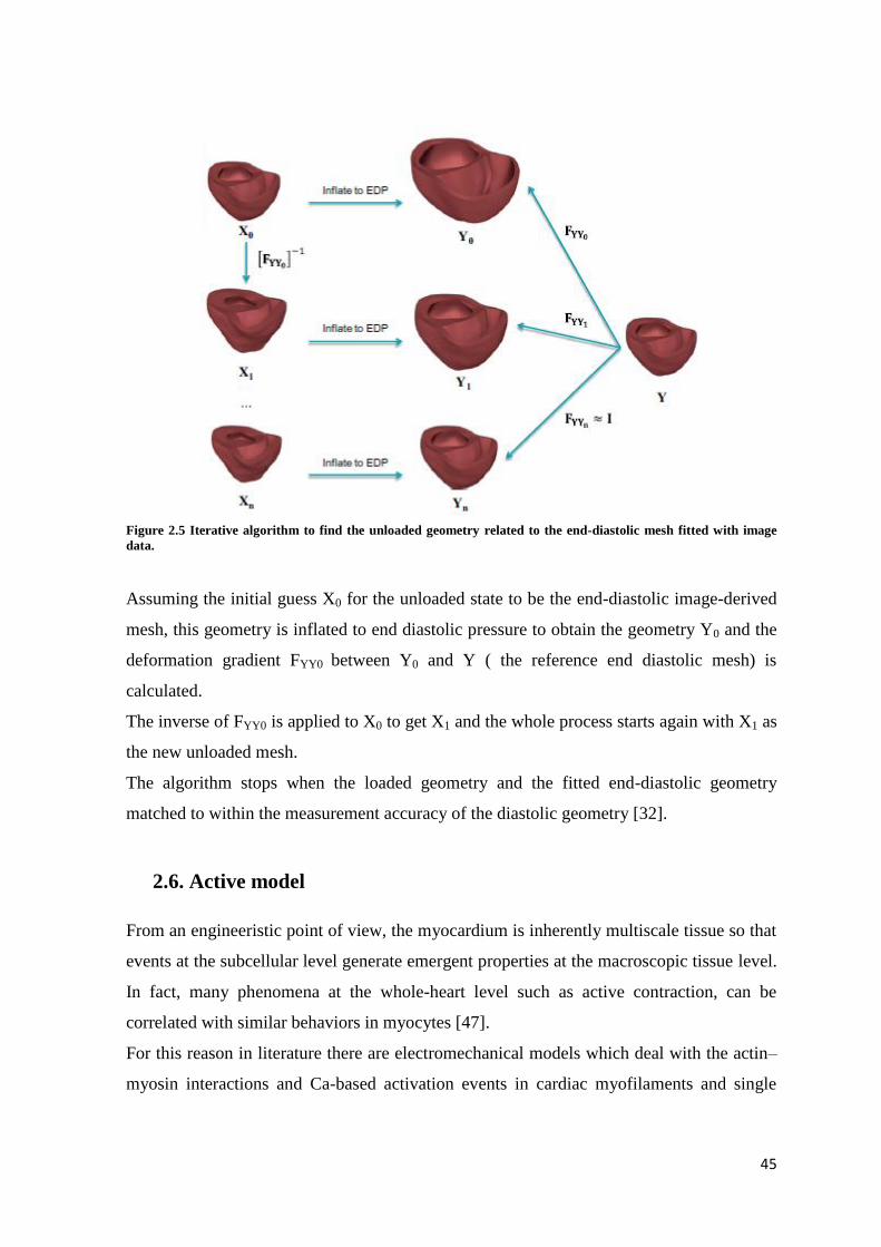
45
Figure 2.5 Iterative algorithm to find the unloaded geometry related to the end-diastolic mesh fitted with image
data.
Assuming the initial guess X0 for the unloaded state to be the end-diastolic image-derived
mesh, this geometry is inflated to end diastolic pressure to obtain the geometry Y0 and the
deformation gradient FYY0 between Y0 and Y ( the reference end diastolic mesh) is
calculated.
The inverse of FYY0 is applied to X0 to get X1 and the whole process starts again with X1 as
the new unloaded mesh.
The algorithm stops when the loaded geometry and the fitted end-diastolic geometry
matched to within the measurement accuracy of the diastolic geometry [32].
2.6. Active model
From an engineeristic point of view, the myocardium is inherently multiscale tissue so that
events at the subcellular level generate emergent properties at the macroscopic tissue level.
In fact, many phenomena at the whole-heart level such as active contraction, can be
correlated with similar behaviors in myocytes [47].
For this reason in literature there are electromechanical models which deal with the actin–
myosin interactions and Ca-based activation events in cardiac myofilaments and single
46
cells; consequently, the myofilament and single-cell EM models are applied in the organ-
level models. Since this project faces at the whole organ, the main focus is on models that
are amenable to be extended from cell to organ cardiac models.
Multiscale EM modeling at the organ-level requires solution of coupled electrical and
mechanical components. The electrical component simulates the propagation of a wave of
transmembrane potential by solving a reaction–diffusion system.
For the mechanical component, active tension generated by the myocytes is used to
compute the deformation of the organ, as described by continuum mechanics with the
myocardium being a transversely isotropic, hyper- elastic, and nearly incompressible
material with passive properties defined by an exponential strain energy function [47].
In this work the models include only the mechanical component of the active stress without
electrical coupling.
Simultaneous solution of the myofilament model equations with those representing passive
cardiac mechanics over the volume of the heart constitutes simulation of cardiac
contraction.
A number of models of active tension development in cardiac muscle have been proposed.
In essence they may be grouped into three categories [48]:
1) time-varying elastance models that include the essential dependence of cardiac active
force development on muscle length and time;
2) “Hill” models, hyperbolic force-velocity relation yields to a reduced fiber tension by
increased shortening velocity; according to the three elements model, the sarcomere is
modeled as a passive element in parallel with a series combination of a contractile element
and series elastic element;
3) fully history-dependent models, either based on system of partial differential equations
as functions of time and cross-bridge position, or on myofilament activation models which
yields a system of ordinary differential equations as functions of time and shortening
velocity.
In this project, the generation of active stress in the fiber direction was calculated by the
Arts model of sarcomere mechanics [6], in which the length of the contractile element
(Lsc) and a time-variant contractility parameter (C) were state variables (for equations see
Appendix) and the shortening velocity and force function is based on Hill model.

47
Active fiber stress σf,a is calculated by:
σ𝑓, 𝑎 = σ𝑎𝑐𝑡 ∗ 𝐶 ∗ (𝐿𝑠𝑐 − 𝐿𝑠𝑐0) ∗ (𝐿𝑠−𝐿𝑠𝑐0
𝐿𝑠𝑒,𝑖𝑠𝑜) (5)
With 𝜎act as active stress scaling factor, Ls sarcomere length and Lse,iso length of the
series elastic element during isometric contraction (subscript number “0” refers to the
initial time). The other two components (sheet and normal sheet directions) of the active
stress are derived from σf,a multiplied by a scaling factor (see Appendix).
Hence, systolic contraction is modelled by defining the total second Piola-Kirchhoff stress
tensor Stot as the sum of the passive three-dimensional stress tensor Spass derived from
the Cauchy stress (3, 4) and an active three-dimensional stress tensor Sact . Accordingly,
the total Piola-Kirchhoff stress tensor Stot:
𝑆𝑡𝑜𝑡 = 𝑆𝑝𝑎𝑠𝑠 + 𝑆𝑎𝑐𝑡 (6)
Where each contribution terms Spass and Sact are driven out from the following formulas
(see Appendix) :
𝑆𝑝𝑎𝑠𝑠 = 𝐽𝐹−1 ∗ 𝜎𝑝𝑎𝑠𝑠 ∗ 𝐹𝑇
𝑆𝑎𝑐𝑡 = 𝑀𝑎𝑡𝑟𝑖𝑥([[𝑡𝑐11,0,0], [0, 𝑡𝑐22,0], [0,0, 𝑡𝑐33]])
2.7. Circulatory model
Patient-specific simulation requires that a wide variety of measurements can be combined
to estimate the mechanical and hemodynamic status of heart and circulation as a whole.
For that purpose, models of heart chamber, blood vessels, and valve have to be integrated
into a comprehensive model.
In literature many models have been proposed from the simulation of the closed-loop
circulation on a beat-to-beat basis. All these models suffer from the major problem that
uncertainties of the parameter values in each subsystem add up to such a high level of
overall inaccuracy that the reliability of the simulation is severely affected [49].
48
The main issue is to provide a realistic measurement for all of these parameters and this
aspect is hardly satisfied with clinical common methods. The number of parameters with
patient-specific values should be limited, while the simulation as a whole should still be
realistic.
This project makes use of the modular-based circulatory and hemodynamic system: the
CircAdapt model proposed by Arts at al [50].
The CircAdapt model was designed to simulate beat-to-beat dynamics of the four-chamber
heart with systemic and pulmonary circulation while incorporating a realistic relation
between pressure-volume load and tissue mechanics and adaptation of tissues to
mechanical load.
In this model, the whole circulation is composed of four module types, such as compliant
blood vessels, actively contracting chambers, valves with inertia, and peripheral
resistances.
In the basic version of the CircAdapt model, the ventricular section is described by the
TriSeg model [51], where left ventricular free wall, septum, and right ventricular wall meet
in a common junction line, thus forming left and right ventricular cavity.
Furthermore, the whole heart is encapsulated in an elastic pericardial chamber [Figure
2.6a]. Atria and ventricles are represented by chambers having a wall, composed of
contractile myocardial tissue. Large arteries and veins are represented by nonlinearly
elastic tubes that can conduct pressure waves. Tubes and chambers can be connected by
valves, whose effective orifice area depends on direction and magnitude of flow through
the valve and on pressure drop over the valve. Peripheral vascular beds of the various
organs may be simulated by a resistance connecting the arterial module to the venous
module. Besides organs, tissues may also be handled as modules. Myocardial tissue is
simulated by a nonlinearly elastic material harboring myofibers that contract after
depolarization. Vascular tissue is considered nonlinearly elastic.
Sections of the CircAdapt model can be replaced easily. For example, when incorporating
a finite element model of the left ventricle as a module, first both ventricles are handled as
uncoupled chambers [Figure 2.6b], thus readily neglecting direct mechanical ventricular
interaction. For a chamber, the CircAdapt model requires cavity pressure to be known as a
function of volume only. Next, the single left ventricular chamber can be replaced by a
finite element model of that chamber. The latter module should be designed so that

49
pressure is delivered as a function of cavity volume [Figure 2.6c]. The sequence of
depolarization is modeled by a set of delay times for electrical conduction [Figure 2.6d]. In
a more sophisticated ventricular section, the pair of ventricles can be replaced by a finite
element model of the coupled ventricles [Figure 2.6e]. Furthermore, the simple description
of the whole systemic circulation [Figure 2.6f] may be replaced by a realistic tree of
arteries and veins feeding and draining the different organs, respectively.
The modular setup is advantageous because the various modules such as blood vessels and
chambers are composed of a few types of tissues. Parameters related to the tissue are
therefore largely general, resulting in great reduction of the number of unknown
parameters. An important problem remains, however. Geometry of the different
components of the circulatory system varies per individual. Accurate measurement of all
these dimensions is complicated in a regular clinical setting .
For this reason, whenever direct measurement are not available, human cardiac
measurement are supplemented with empirical data [32].
Figure 2.6 Modular setup to model the complete circulation. (a) The CircAdapt model describes pressures and
flows in heart and circulation. L/R A/V = left/right atrium/ ventricle; peri = pericardium; sys, pulm = systemic,
pulmonary circulation.
Four modules are used, i.e., contractile chambers, nonlinearly elastic tubes, valves, and peripheral resistances. The
TriSeg module describes LV–RV interaction. (b) To prepare incorporation of a finite element model of the left
ventricle, the TriSeg module may be replaced by simpler, but less accurate independent ventricles. (c) Based on
(b), the LV may be replaced by the finite element model. (d) The sequence of electrical depolarization may be
included. SA, AV = sinoatrial and atrioventricular nodes. (e) Replacement of the TriSeg module by a finite
element representation of both coupled ventricles. (f) Replacement of the single-channel systemic circulation
module by a more complex, multiple organ representation.

50
2.8. Modeling of a Pathological Heart
Simulations carried out with patient specific modeling can help researchers understand the
mechanical behavior of the heart under different disease conditions.
For patients affected by left ventricular dyssynchrony with or without scar region in
myocardial tissue, becomes an outstanding matter to characterize the PS model with an
electrical activation time pattern which represents the conduction impulse in the ventricles
and material properties adapted to an infarcted tissue.
In literature some studies showed the electromechanical delay in LBBB patients using
computational models [53].
Constantino et al. presents a 3D maps of electrical activation (left) and the onset of
myofiber shortening (middle) in both short- and long-axis views during LBBB for
nonfailing and HF ventricles. In both non-failing and HF dyssynchronous ventricles,
depolarization began at the right ventricular septal and free wall and propagated toward the
LV lateral wall. Mechanical activation followed the direction of depolarization. They
established that the propagation of mechanical activity was slower in the HF model [Figure
2.7].
Usually a scar region affecting the myocardial tissue due to a heart attack presents stiffer
mechanical properties [54, 65]. This aspect have be included in the values describing the
strain energy function of the constitutive model.
Figure 2.7 Activation time distribution in non-failing and failing heart

51
2.9. Patient Specific Mechanical Models in Literature
The typical sections of cardiac 3D models described in previous sections are assembled to
create a cardiac mechanical model. This describes the deformation of the heart during the
cardiac cycle determined by the mechanical equilibrium between forces developed by
myofibres active contraction, passive stretch of the connective tissue matrix, pressure in
the cardiac cavities and pressure exerted by the pericardium.
Looking at the literature, mechanical biventricular model of the heart have been raised
providing significant and reliable information about the mechanical interaction between the
two ventricles for CRT patients [60]. For example, Lumens et al. provided a novel insights
in the working mechanism of CRT, investigating the consequences of left ventricular and
biventricular pacing for local LV and RV tissue mechanics. They showed for the first time
in patients that pacing-induced hemodynamic improvement can occur without electrical
resynchronization. These findings were corroborated by computer simulations, showing
that both pacing strategies increase total ventricular myofiber work to a similar extent, yet
differently redistribute myofiber load over the LV and RV myocardium [61].
With a more detailed deformation analysis in 3D, Niederer et al. developed a model linking
deformation, pressure and electrical activation data with integrative calculations of
regional cardiac work. Through this method they were able to investigate the underlying
changes in cardiac function that produce changes in regional work observed following
CRT [62].
Other groups published studies inherent to LBBB patient using computational models; the
purposes always aimed to a better insight of causes and consequence of the pathology
(Vernooy 2004, Prinzen 1999).
Even if historically the development of electrophysiological and mechanical models of
cardiac function proceeded rather independently than in tandem, during the last decades
researchers tried to couple existing models of cellular electrophysiology and active
mechanics in a unique electromechanical model [Figure 2.8] [47].
Whole-heart models of cardiac electromechanics have been used to study the influence of
local disturbances in electrical propagation or cellular electrophysiological pathologies on
regional contraction and global heart function [66].

52
Figure 2.8 A) Schematic of the general approach to modeling cardiac EM function. (B) Geometrical models of the
heart. (C) Computational meshes of the canine heart for the electrical and mechanical problems. (D) Fiber and
sheet orientations obtained from DTMR imaging of the canine heart.
2.9.1. CT as Gold Standard Imaging Driver for PS Computational Models
Since the innovative aspect of the study is the employment of Echocardiography imaging,
this project considers Krishnamurthy &Co. study [32] as the main reference since the
authors derived the Patient Specific cardiac model from CT, the gold standard imaging
technique for cardiac anatomy reconstruction. In fact, this one of the most used for
capturing patient specific anatomy thanks to its high spatial resolution.
In particular, three-dimensional bi-ventricular geometry was segmented from cardiac CT
images at end-diastole from patients with heart failure. Human myofiber and sheet
architecture was modeled using eigenvectors computed from diffusion tensor MR images
from an isolated, fixed human organ-donor heart and transformed to the patient-specific
geometric model using large deformation diffeomorphic mapping. They presented new
methods for patient specific passive/active material properties assessment. In this term the
Ogden Holzepfel parameters were adjusted to match the empirical human pressure-
volume relation reported by Klotz [46]. On the other hand, cardiac catheterization
measurement was used to define active material properties of the Hill-type contractile
model. Also circulatory model values based on CircAdapt model were modified in order to
match clinical measurements. In this way the authors developed an integrated multi-scale

53
patient-specific model of the heart that includes a geometric 3D finite-element bi-
ventricular component, a material model of the myocardium that incorporates fiber
architecture, an active contractile component, and a lumped-parameter hemodynamic
component for the circulation. The validation of the model was carried out though the
comparison between simulated results and clinical data.

54
3. MATERIALS AND METHODS
55
3.1. Project Approach and Workflow
The study herein presented focuses on the implementation of patient-specific (PS)
biventricular models from ultrasound imaging, and on their application to the analysis of
the cardiac mechanics in a small cohort of patients suffering from heart failure due to left
ventricular dysfunction and complicated by myocardial infarction.
The implementation of these PS models involves the definition of four key aspects, as
described in chapter 2: i) the definition of the patient-specific ventricular anatomical
model, ii) the definition of the passive mechanical properties of myocardial tissue, iii) the
definition of the contractile properties of myocardial tissue, and iv) the setting of a lumped-
parameter model describing the hydraulic behavior of the circulatory system to be coupled
to the biventricular model to obtain proper boundary conditions [Figure 3.1].
The anatomical model of the ventricles consists of i) the unloaded ventricular geometry, ii)
a volumetric scalar field representing the scar region within the ventricular wall, and iii) a
fiber-sheet local material coordinate system that defines the organization of myocardial
tissue into sheets and of myofibers within each sheet. The biventricular geometry is
reconstructed from 2D ultrasound imaging at the end diastolic state and discretized into
3D hexahedral cubicHermite finite elements (128 elements, 209 nodes). Since at the end
diastolic state the ventricles are not unloaded, their reference and stress-free configuration
has to be identified through a previously implemented unloading algorithm [32].
Local fiber architecture is represented by a local myofiber-sheet material coordinate
system.
The constitutive modeling of myocardial tissue is based on the description of its passive
stress-strain behavior though the well-known Ogden-Holzapfel strain energy function, with
the addition of a volumetric term to account for some degree of tissue compressibility.
Muscle contraction is described through a Hill model. The parameters characterizing the
two aspects of myocardial properties are properly altered in the scar region to simulate the
locally altered behavior of the ventricular wall, as explained in section 3.3.4.
Boundary conditions of two types are defined on the models. On the one hand, kinematic
constraints are defined to prevent from rotations of the ventricular base, as well as from its
displacement along the ventricles long axis. On the other hand, the intraventricular
56
pressures are coupled to the inward/outward blood flow, and hence to the time-dependent
intraventricular volumes, by means of a lumped-parameter model of the circulation,
namely the CircAdapt circulatory model.
In order to study the accuracy and reliability of the models, the results of the present study
were compared to clinical measurements, and to the results of Krishnamurthy’s models. He
previously developed cardiac models on the same cohort of patients, making use of CT
images. For this reason in this thesis, his study is frequently named as “CT model” for the
sake of simplicity (part of his work can be found in [32]).
Summarizing, the following chapter describes the 5 steps that brought to the formulation of
the models, namely [Figure 3.1]:
Biventricular mesh creation: includes endo and epicardial profiles tracing from echo-
images with ImageJ. This step is followed by a manual fitting in Blender in order to
adjust the mesh template to the patient-specific profiles;
Patient-Specific (PS) model implementation in Continuity: after a further automatic
data fitting and mesh refinement, PS features (such as scar region and activation time
pattern) and biomechanical forms are included in the model ;
Unloaded Geometry: an unloaded mesh is estimated by Krishnamurthy’s algorithm in
order to compute stresses correctly;
Full-Beat Simulation: the closed loop circulatory model is coupled to the finite element
ventricular model to simulate complete cardiac cycles ;
Hemodynamic and Local Work Analysis: comparison with clinical and CT model.
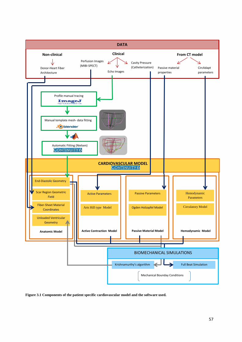
57
Manual template mesh- data fitting
Profile manual tracing
From CT model Non-clinical Clinical
Echo Images
Cavity Pressure
(Catheterization)
Perfusion Images
(MIBI-SPECT) Donor-Heart Fiber
Architecture
CircAdapt
parameters
Passive material
properties
CARDIOVASCULAR MODEL
Automatic Fitting (Nielsen)
End-Diastolic Geometry
Scar Region Geometric
Field
Fiber-Sheet Material
Coordinates
Unloaded Ventricular
Geometry
Anatomic Model Passive Material Model Active Contraction Model Hemodynamic Model
Passive Parameters
Ogden Holzapfel Model
Active Parameters
Arts Hill type Model
Hemodynamic
Parameters
Circulatory Model
BIOMECHANICAL SIMULATIONS
Krishnamurthy’s algorithm Full Beat Simulation
DATA
Mechanical Bounday Conditions
Figure 3.1 Components of the patient specific cardiovascular model and the software used.
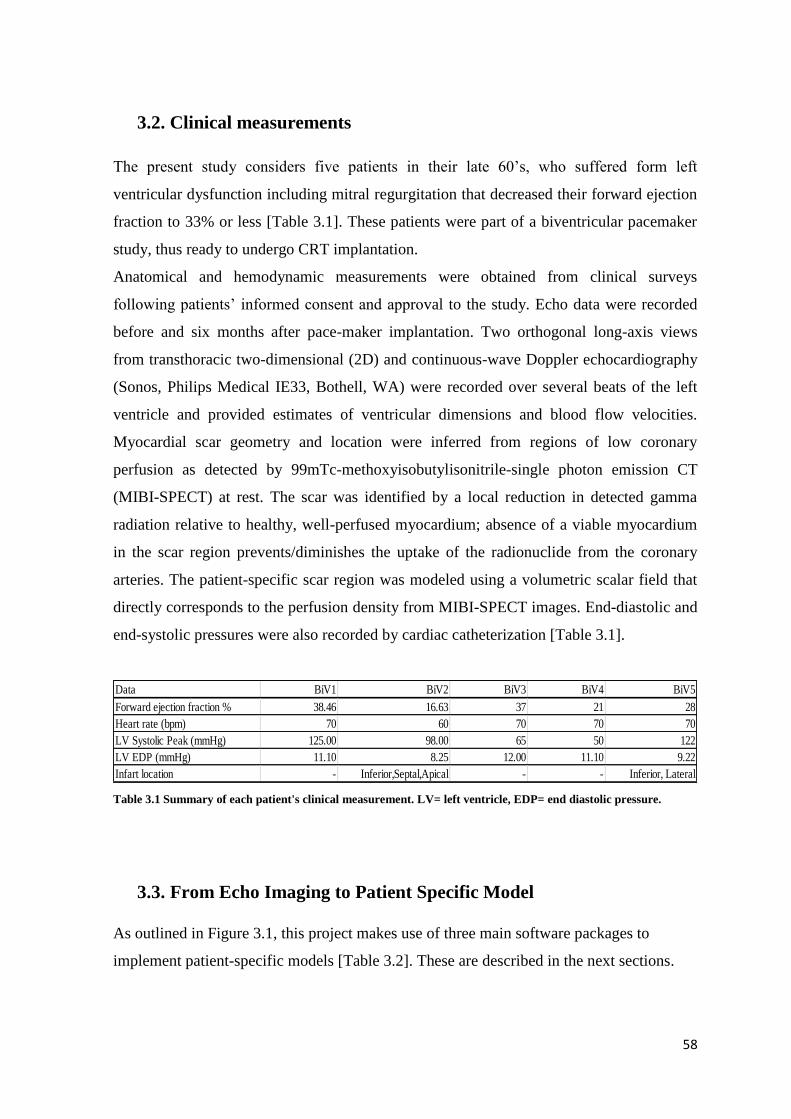
58
3.2. Clinical measurements
The present study considers five patients in their late 60’s, who suffered form left
ventricular dysfunction including mitral regurgitation that decreased their forward ejection
fraction to 33% or less [Table 3.1]. These patients were part of a biventricular pacemaker
study, thus ready to undergo CRT implantation.
Anatomical and hemodynamic measurements were obtained from clinical surveys
following patients’ informed consent and approval to the study. Echo data were recorded
before and six months after pace-maker implantation. Two orthogonal long-axis views
from transthoracic two-dimensional (2D) and continuous-wave Doppler echocardiography
(Sonos, Philips Medical IE33, Bothell, WA) were recorded over several beats of the left
ventricle and provided estimates of ventricular dimensions and blood flow velocities.
Myocardial scar geometry and location were inferred from regions of low coronary
perfusion as detected by 99mTc-methoxyisobutylisonitrile-single photon emission CT
(MIBI-SPECT) at rest. The scar was identified by a local reduction in detected gamma
radiation relative to healthy, well-perfused myocardium; absence of a viable myocardium
in the scar region prevents/diminishes the uptake of the radionuclide from the coronary
arteries. The patient-specific scar region was modeled using a volumetric scalar field that
directly corresponds to the perfusion density from MIBI-SPECT images. End-diastolic and
end-systolic pressures were also recorded by cardiac catheterization [Table 3.1].
Table 3.1 Summary of each patient's clinical measurement. LV= left ventricle, EDP= end diastolic pressure.
3.3. From Echo Imaging to Patient Specific Model
As outlined in Figure 3.1, this project makes use of three main software packages to
implement patient-specific models [Table 3.2]. These are described in the next sections.
BiV1 BiV2 BiV3 BiV4 BiV5
38.46 16.63 37 21 28
70 60 70 70 70
125.00 98.00 65 50 122
11.10 8.25 12.00 11.10 9.22
- Inferior,Septal,Apical - - Inferior, Lateral
LV Systolic Peak (mmHg)
LV EDP (mmHg)
Data
Forward ejection fraction %
Heart rate (bpm)
Infart location

59
Software Function
Image J Endo/Epicardial profile tracing on Echo images
Blender™ Manual template mesh-data fitting
Matlab® Coordinate systems transformation
Continuity
Nielsen automatic Mesh-Data Fitting
Mesh refinement
Biomechanical Simulations
Table 3.2 List of software used in this study for patient specific model development.
3.3.1. Image J
ImageJ is an open source image processing software designed for different formats of
scientific multidimensional images.
It supports standard image processing functions such as logical and arithmetical operations
between images, contrast manipulation, convolution, Fourier analysis, sharpening,
smoothing, edge detection, and median filtering. It does geometric transformations such as
scaling, rotation, and flips. This software was used to detect endo and epicardial profiles on
ultrasound images.
This action was required for identifying patient-specific anatomy; in fact, as described
further on in this thesis, the generic mesh template, fitted on these traced profiles, is the
base for the patient-specific model.
For each patient two views were considered: a long-axis two-chamber (TC) view and four-
chamber (FC) view . It was assumed that the two views were imaged perpendicularly.
Endocardial and epicardial contours were manually traced on the two images through the
“Segmented-line” function. On the TC view, only the contours of the left ventricle were
traced, on the FC the contours of both ventricles were traced. Traced points were
automatic interpolation which converts the traced selection into a sub-pixel resolution ROI
of floating-point coordinates spaced 0.5 pixels apart [Figure 3.2].
The XY coordinates of the obtained points expressed in pixels were exported in a .xls file
and opened in Excel. The pixel distance (in cm) between two white dots on the border of
the angle view on the ultrasound image was used to scale pixel coordinates to cm
coordinates [Figure 3.2].

60
Figure 3.2 Upper Panel - Manual segmentation of myocardial profile (FC view). Lower Panel - Automatic
interpolation on traced profile: number of points increased, smoothing the profile contours. Zoom out on white
dots distance for real measurements.
3.3.2. Blender™ (version 2.49b)
Blender was delivered as a usable product in August 1994 as an integrated application that
allows the creation of a broad range of 2D and 3D content. Blender provides a wide
spectrum of modeling, texturing, lighting, animation and video post-processing
functionality.
In this project, the use of Blender was limited to the manual adaptation of a template-mesh
on the imported patient-specific cardiac profiles. In order to carry out this operation, endo-
and epicardial profiles were manually co-registered to recreate the three-dimensionality of
the organ. To this aim, two reference regions were matched in the two views: the left
ventricular apex and the plane containing the right ventricle profiles, which has to cut in
two the left ventricle in the complementary view [Figure 3.3]. This criterion is only semi-
quantitative, ant it application largely depends on the operator.

61
Figure 3.3 Co-registration of endocardial and epicardial profiles obtained from two-chambers and four-chambers
views.
As already mentioned, the first fitting between mesh template and ventricular profiles was
manual. In order to simplify this step, a basic mesh previously created and available in the
CMRG (Cardiac Mechanic Research Group) database was used as template. This is a
generic 2D linear Lagrangian biventricular template mesh with 50 vertexes and 40 faces
with four nested surfaces representing the endocardial and epicardial surfaces of the left
ventricle, right ventricle, septum and epicardium [Figure 3.4A].
Nodal coordinates were defined in a cartesian reference frame having the origin of the X
axis at half the height of the mesh in the XY plane, with the Z axis on the half of depth in
ZX plane. The three nodes corresponding to the LV apex lie along the X axis [Figure
3.4.C].
First, the template is rescaled increasing or decreasing dimensions to make it
approximately similar to the data profiles. A refinement is carried out moving the mesh
boundaries node by node [Figure 3.4B]. Every node is properly translated without dis-
aligning vertexes and creating future coarse and sharp edges in the mesh [Figure 3.4D].
Once the manual fitting is concluded, the mesh is saved and exported as .OFF file.

62
3.3.3. Matlab® (The Mathworks, Inc.)
MATLAB is a well-known coding environment that allows to easily handle vectors and
matrices allows for an extremely natural way to express computational mathematics. In
this work, a pre-existent Matlab script available in the CMRG lab’s file archive was
exploited to apply the transformation of mesh coordinate system. This conversion was
necessary to compute the second automatic mesh-data fitting base on Nielsen’s algorithm.
Nielsen’s mathematical method works on prolate spheroidal coordinate system and applies
least square fitting procedure only on the radial coordinate (μ) [see paragraph 2.2].
In order to transform the nodal coordinates of the mesh yielded by Blender (see section
3.3.2) from cartesian to prolate spheroidal coordinate system, the general definition of
prolate spheroidal coordinates was used (μ,ѵ, Φ):
𝑥 = 𝑎 ∗ 𝑠𝑖𝑛ℎµ ∗ 𝑠𝑖𝑛ѵ ∗ 𝑐𝑜𝑠𝛷
𝑦 = 𝑎 ∗ 𝑠𝑖𝑛ℎµ ∗ 𝑠𝑖𝑛ѵ ∗ 𝑠𝑖𝑛𝛷
A)
B) D)
C)
Figure 3.4 Blender workspace A) In “Object mode” three layer mesh, each apex lies on X axis (red line) B) “Edit
mode” mesh texture C) Section on XY plane: left ventricle apexes aligned on X axis D) Focus on one single vertex
selection for setting a new position closer to data points.
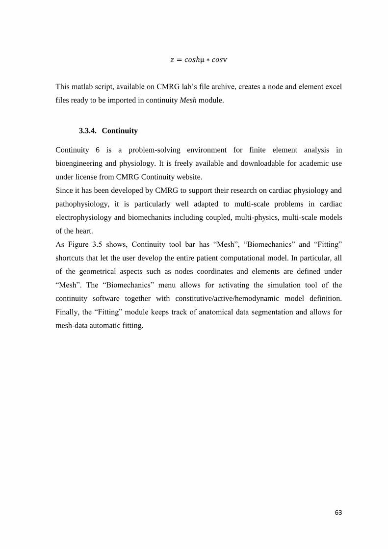
63
𝑧 = 𝑐𝑜𝑠ℎµ ∗ 𝑐𝑜𝑠ѵ
This matlab script, available on CMRG lab’s file archive, creates a node and element excel
files ready to be imported in continuity Mesh module.
3.3.4. Continuity
Continuity 6 is a problem-solving environment for finite element analysis in
bioengineering and physiology. It is freely available and downloadable for academic use
under license from CMRG Continuity website.
Since it has been developed by CMRG to support their research on cardiac physiology and
pathophysiology, it is particularly well adapted to multi-scale problems in cardiac
electrophysiology and biomechanics including coupled, multi-physics, multi-scale models
of the heart.
As Figure 3.5 shows, Continuity tool bar has “Mesh”, “Biomechanics” and “Fitting”
shortcuts that let the user develop the entire patient computational model. In particular, all
of the geometrical aspects such as nodes coordinates and elements are defined under
“Mesh”. The “Biomechanics” menu allows for activating the simulation tool of the
continuity software together with constitutive/active/hemodynamic model definition.
Finally, the “Fitting” module keeps track of anatomical data segmentation and allows for
mesh-data automatic fitting.
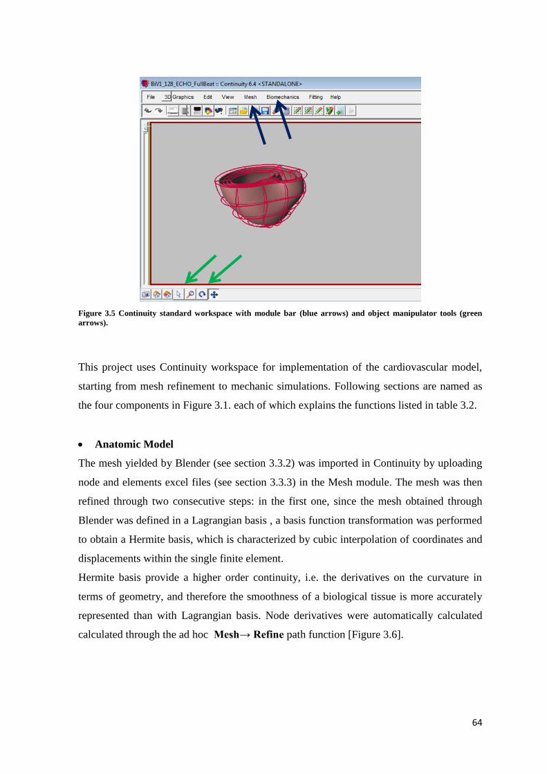
64
Figure 3.5 Continuity standard workspace with module bar (blue arrows) and object manipulator tools (green
arrows).
This project uses Continuity workspace for implementation of the cardiovascular model,
starting from mesh refinement to mechanic simulations. Following sections are named as
the four components in Figure 3.1. each of which explains the functions listed in table 3.2.
Anatomic Model
The mesh yielded by Blender (see section 3.3.2) was imported in Continuity by uploading
node and elements excel files (see section 3.3.3) in the Mesh module. The mesh was then
refined through two consecutive steps: in the first one, since the mesh obtained through
Blender was defined in a Lagrangian basis , a basis function transformation was performed
to obtain a Hermite basis, which is characterized by cubic interpolation of coordinates and
displacements within the single finite element.
Hermite basis provide a higher order continuity, i.e. the derivatives on the curvature in
terms of geometry, and therefore the smoothness of a biological tissue is more accurately
represented than with Lagrangian basis. Node derivatives were automatically calculated
calculated through the ad hoc Mesh→ Refine path function [Figure 3.6].

65
Figure 3.6 2D element mesh in prolate coordinate system: Lagrangian (left) and Hermite basis (right). The red
mesh is obtained with an automatic function for derivatives calculation. With Hermite basis mesh edges are
smoothed, showing a closer representation for a biological tissue.
In the second refinement step, the Nielsen automatic fitting algorithm [26] was applied
through the Fit Data function in the Fitting Module. This algorithm implies the iterative
modification of the nodal coordinates of the mesh; based on previous experience developed
in the CMRG lab, ten refinement iterations were run to correctly fit the patient-specific
data points, i.e. the sampled profiles of the endocardium and epicardium of the left and
right ventricle, respectively [Figure 3.7, top panel]. Local mismatches between the fitted
mesh and image-based profiles were sub-millimetric [Figure 3.7, bottom panel].
The fitted prolate spheroidal, consisting of 2D surface elements, was converted to a 3D
hexaedral cubic-Hermite topology, consisting of 3D elements defined in Cartesian
coordinates. The converted mesh was refined to a resolution of 128 elements and 209
nodes [Figure 3.8].

66
Figure 3.7 Continuity Fitting module. Top panel: data points (black) obtained from echo profiles. The mesh prior
to applying data fitting is depicted in blue. Mid panel: the fitted mesh is depicted in red. Local mismatches vs.
image-based data are represented; in the color map, blue corresponds to the worst mismatches (0.65 mm in this
example), red corresponds to the minimal mismatch (0 mm in this example).
Figure 3.8 Example of 3D cubic-Hermite biventricular mesh in Cartesian coordinates in Continuity workspace.
In the node form, the fiber architecture is imported as a scalar field. This study bases on the
assumption of fiber architecture preservation among individuals [63]. Measurements came
0 0.65
67
from a donor human heart and fibers have been modeled in a patient-specific anatomy,
after accounting for the variations in fiber orientation due to differences in ventricle size
and shape [32].
Two of the five patients had a myocardial infarction. Figure 3.9 shows the scar distribution
on the end-diastolic mesh. The red regions correspond to infarcted tissue.
Figure 3.9 Scar region representation for patient #2 and #5. Reference number are adimensional, deriving from
MIBI-Spect exam. The higher value correspond to infarcted tissue.
Passive Material Model
As far as its passive stress-strain response is concerned, the myocardium was assumed as a
transversely isotropic slightly compressible material. The invariant-based global strain
-0.5
1
0
0.12
Patient 2
Location: Inferior, Septal, Apical
Patient 5
Location: Inferior, Lateral

68
energy function proposed by Ogden and Holzapfel [9] was used. This function is
composed by an isochoric (i.e. deviatoric) and a volumetric part.
Ψiso = 𝑎
2𝑏𝑒𝑏(𝐼1−3) +
𝑎𝑓
2𝑏𝑓{𝑒𝑏𝑓(𝐼4𝑓−1)2
− 1}
The value of the constitutive parameters for pathologic myocardium were defined by
averaging the values reported by Krishnamurthy’s study [32] [Table 3.3]. In this previous
project, the patient specific values have been modified from the default group in order to
match the computed passive curve with the empirical Klotz model (Chapter 2, paragr. 2.4).
Table 3.3 Constitutive model parameters. Echo values are average of CT values.
In order to mimic the effects of the presence of a scar, the stiffness a was increased by a
factor of 10 [65].
The volumetric part Ψvol(J) comes from the following equation:
𝚿vol(J) = K(J − 1) ∗ ln(𝐽) /2
With K the bulk modulus. Bulk modulus value was set to 350kPa for all the patients
according to Kerckhoffs et al. [64] (for detailed equations see Appendix).
Active contraction Model
The active contraction of myocardial tissue was modeled in order to simulate ventricular
biomechanics during the systolic phase of the cardiac beat. To this aim, the Arts model was
adopted, where the shortening rate of the contractile element is described modifying the
approach by Lumens et al. [51, theory in Chapter 2, section 2.6]. This yields a hyperbolic
Hill-relation between shortening rate and contractile force. The governing ordinary
differential equations yielding the dependent variables (Lsc sarcomere length, C time-
variant contractility) are the following:
Default CT pat 1 CT pat 2 CT pat 3 CT pat 4 CT pat 5 Echo
a (kPa) 2.28 0.912 0.912 0.684 0.684 0.684 0.7752
af (kPa) 1.68 0.674 0.674 0.51 0.51 0.51 0.5756
b 9.72 8.75 8.26 9.72 9.72 9.72 9.239
bf 15.77 14.201 13.42 15.77 15.77 15.77 14.9846

69
The two parameters L0 (contractile element length at zero active stress) and C0 (diastolic
contractility level ) at t=0 were set to2 µm and 0.0 respectively. Specific parameters and
equations are collected in Appendix. The active patient specific parameters were imported
from the CT model. Originally, the author identified the set of constitutive parameters by
simulating the isovolumetric contraction with the biventricular mesh and adjusting them
so that computed intraventricular pressure values matched experimental values measured
through a catheter [32].
In order to simulate the presence of the scar region, the stress scaling factor σact is
decreased by an order of magnitude where there is the scar tissue [65].
The time activation pattern is a patient specific distribution already available from the CT
model. Table 3.4 shows for each patient the mesh region where the pacing takes place.
These data reflect the LBBB effect: commonly, the left ventricle is the last region to be
depolarized [60].
Table 3.4 Location of pacing during the active contraction. These data reflects LBBB pathology: left ventricle is
the last area to be activated.
An example of time activation distribution on end diastolic fitted mesh is shown in Figure
3.10 for patients #2 and #3.
dLsc
dt
LsNorm -1
bhill LsNorm +1vmax LsNorm 1
LsNorm -1
bHill LsNorm +1vmax e
aHill (LsNorm1) LsNorm 1
dC
dt1
r CL f rise
1
dCrest C
1 e(T t )/d
1 2 3 4 5
Activation Pattern RVFW RVFW Septum Septum RVFW
Patient
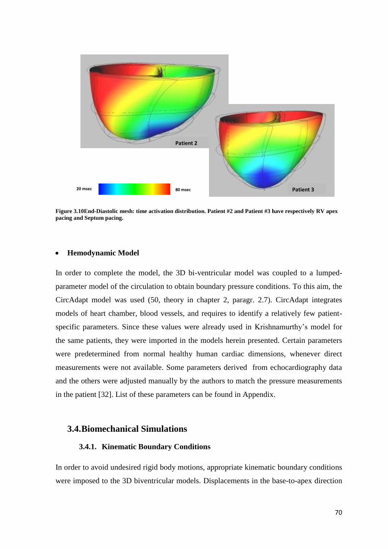
70
Figure 3.10End-Diastolic mesh: time activation distribution. Patient #2 and Patient #3 have respectively RV apex
pacing and Septum pacing.
Hemodynamic Model
In order to complete the model, the 3D bi-ventricular model was coupled to a lumped-
parameter model of the circulation to obtain boundary pressure conditions. To this aim, the
CircAdapt model was used (50, theory in chapter 2, paragr. 2.7). CircAdapt integrates
models of heart chamber, blood vessels, and requires to identify a relatively few patient-
specific parameters. Since these values were already used in Krishnamurthy’s model for
the same patients, they were imported in the models herein presented. Certain parameters
were predetermined from normal healthy human cardiac dimensions, whenever direct
measurements were not available. Some parameters derived from echocardiography data
and the others were adjusted manually by the authors to match the pressure measurements
in the patient [32]. List of these parameters can be found in Appendix.
3.4. Biomechanical Simulations
3.4.1. Kinematic Boundary Conditions
In order to avoid undesired rigid body motions, appropriate kinematic boundary conditions
were imposed to the 3D biventricular models. Displacements in the base-to-apex direction
Patient 2
Patient 3 80 msec 20 msec

71
(i.e. the X axis of the reference frame) of the nodes at the base of the left and right
ventricles were suppressed so to mimic the constraining effects of the presence of the atria,
of the aorta and of the vena cava. Among the basal nodes, for two nodes at right and left
ventricular epicardium free wall were prevented from translating along the Z axis, and two
epicardial nodes at the ventricular junctions were prevented from translating along the Y
axis [Figure 3.11]; in this way, unrealistic motions in the plane perpendicular to the
ventricular long axis were avoided. Furthermore, rotations were suppressed at the apex
[Figure 3.11].
Figure 3.11 Mechanic Boundaries Conditions applied. Nodes at the base fixed along X axis. Junction nodes are
also bounded on Z axis, while freewall nodes also on Y axis. Apex derivatives s(1) blocked in each direction.
Y
X Z
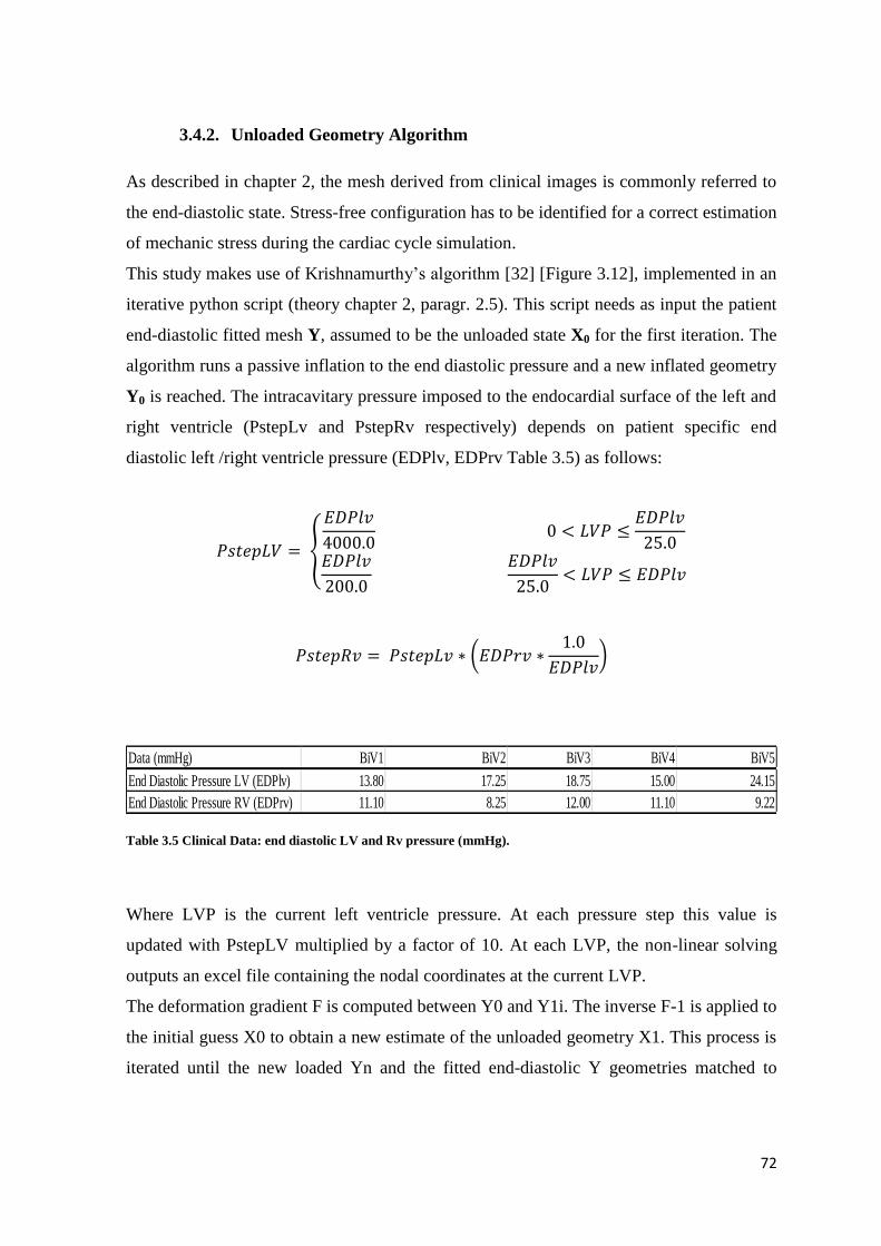
72
3.4.2. Unloaded Geometry Algorithm
As described in chapter 2, the mesh derived from clinical images is commonly referred to
the end-diastolic state. Stress-free configuration has to be identified for a correct estimation
of mechanic stress during the cardiac cycle simulation.
This study makes use of Krishnamurthy’s algorithm [32] [Figure 3.12], implemented in an
iterative python script (theory chapter 2, paragr. 2.5). This script needs as input the patient
end-diastolic fitted mesh Y, assumed to be the unloaded state X0 for the first iteration. The
algorithm runs a passive inflation to the end diastolic pressure and a new inflated geometry
Y0 is reached. The intracavitary pressure imposed to the endocardial surface of the left and
right ventricle (PstepLv and PstepRv respectively) depends on patient specific end
diastolic left /right ventricle pressure (EDPlv, EDPrv Table 3.5) as follows:
𝑃𝑠𝑡𝑒𝑝𝐿𝑉 = {
𝐸𝐷𝑃𝑙𝑣
4000.0 0 < 𝐿𝑉𝑃 ≤
𝐸𝐷𝑃𝑙𝑣
25.0𝐸𝐷𝑃𝑙𝑣
200.0
𝐸𝐷𝑃𝑙𝑣
25.0< 𝐿𝑉𝑃 ≤ 𝐸𝐷𝑃𝑙𝑣
𝑃𝑠𝑡𝑒𝑝𝑅𝑣 = 𝑃𝑠𝑡𝑒𝑝𝐿𝑣 ∗ (𝐸𝐷𝑃𝑟𝑣 ∗1.0
𝐸𝐷𝑃𝑙𝑣)
Table 3.5 Clinical Data: end diastolic LV and Rv pressure (mmHg).
Where LVP is the current left ventricle pressure. At each pressure step this value is
updated with PstepLV multiplied by a factor of 10. At each LVP, the non-linear solving
outputs an excel file containing the nodal coordinates at the current LVP.
The deformation gradient F is computed between Y0 and Y1i. The inverse F-1 is applied to
the initial guess X0 to obtain a new estimate of the unloaded geometry X1. This process is
iterated until the new loaded Yn and the fitted end-diastolic Y geometries matched to
BiV1 BiV2 BiV3 BiV4 BiV5
13.80 17.25 18.75 15.00 24.15
11.10 8.25 12.00 11.10 9.22
Data (mmHg)
End Diastolic Pressure LV (EDPlv)
End Diastolic Pressure RV (EDPrv)
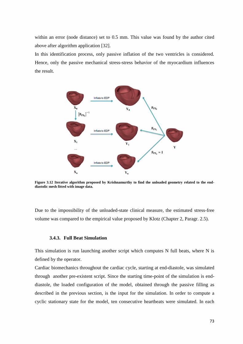
73
within an error (node distance) set to 0.5 mm. This value was found by the author cited
above after algorithm application [32].
In this identification process, only passive inflation of the two ventricles is considered.
Hence, only the passive mechanical stress-stress behavior of the myocardium influences
the result.
Figure 3.12 Iterative algorithm proposed by Krishnamurthy to find the unloaded geometry related to the end-
diastolic mesh fitted with image data.
Due to the impossibility of the unloaded-state clinical measure, the estimated stress-free
volume was compared to the empirical value proposed by Klotz (Chapter 2, Paragr. 2.5).
3.4.3. Full Beat Simulation
This simulation is run launching another script which computes N full beats, where N is
defined by the operator.
Cardiac biomechanics throughout the cardiac cycle, starting at end-diastole, was simulated
through another pre-existent script. Since the starting time-point of the simulation is end-
diastole, the loaded configuration of the model, obtained through the passive filling as
described in the previous section, is the input for the simulation. In order to compute a
cyclic stationary state for the model, ten consecutive heartbeats were simulated. In each

74
heartbeat, the parameters of the active model describing myocardial contraction were
updated. As mentioned in the active contraction model, the activation time pattern was a
patient-specific parameter and was added in the node form as a scalar field.
As far as the parameters of the circulatory model are concerned, initial values were set
accordingly with a Krishnamurthy’s study. Table 3.6 exemplifies this aspect of the
procedure reporting the initial values used for patient#1. The full list of initial values is
reported in the Appendix.
All simulations were run on the CMRG cluster on 32 CPUS with 12 Gb RAM, and
required approximately 72 hours.
Initial Condition Value
time [sec] 0.0
left ventricular pressure [kPa] 1.84
right ventricular pressure [kPa] 1.48
left atrial volume [ml] 27.4
aortic volume [ml] 59.1
vena cava volume [ml] 54.8
right atrial volume [ml] 35.8
pulmonary artery volume [ml] 20.4
pulmonary vein volume [ml] 26.7
aortic valve flow [liter/s] 0
mitral valve flow [liter/s] 0.09
pulmonary artery valve flow [liter/s] 0
tricuspid valve flow [liter/s] 0.15
flow into left atrium [liter/s] -0.03
flow into right atrium [liter/s] -0.03
left atrial contractility [-] 0.83
left atrial contractile element length [m] 1.82
right atrial contractility [-] 0.97
right atrial contractile element length [m] 1.95
Table 3.6 Full Beat Simulation: list of initial condition values for the Circulatory model (CircAdapt). Values refer
to Patient#1 as sample.
3.5. Data and Results Analysis
3.5.1. Echo and Clinical measurement comparison
Simulation results validation against experimental data is necessary in order to assess the
model’s reliability. Through a Matlab® script available in the CMRG database, pressure
and volume data, computed by the full beat simulation in the last simulated cardiac cycle
were compared vs. ground truth data obtained by the direct processing of ultrasound
images and invasive in vivo pressure measurements performed through catheters. In
75
particular, the following indexes were analyzed: maximal contraction velocity index,
minimum contraction velocity index, systolic peak pressure, end systolic volume, end-
diastolic pressure and volume, stroke volume, ejection fraction, stroke work. Of note,
pressure measurements were averaged over multiple heartbeats. Stroke volume and
ejection fraction were derived from volume measured on ultrasound images at end diastolic
and end systolic points. Contractility was estimated based on ECG recordings.
Moreover, as previously mentioned, the cardiac biomechanics of the patients considered in
the present work had already been computed through models whose geometry was based
on CT images. In order to assess the influence of using only two 2D ultrasound images as a
source of anatomical information, results from the models herein presented were compared
to those developed from CT images for the same cohort of patients. A further result
elaboration has been carried out, focusing on the difference and discrepancy of results
coming from two computational ways of cardiac modeling. In particular, for both types of
model stresses and strains during the last cardiac cycle at each Gaussian point in each
element were extracted, and processed through a Matlab® script (available in the CMRG
database) to compute the local work density. Based on this last index, it was possible to
compare Echo and CT models in terms of local work mean, standard deviation and
coefficient of variation related to the mean value. By superimposing the distribution of
local work density and the information on location, shape and extent of the infarcted
region, the effects of dysfunctions in the transmission of the activation potential were
assessed.

76
4. RESULTS AND DISCUSSION

77
4.1. Results and Discussion
This chapter is organized following the project’s sections described in chapter 3: i) post
fitting mesh volume analysis, ii) unloaded geometry and passive inflation curves, iii) full
beat results, iv) hemodynamics, v) local work analysis . Comparisons were made between
the Echo and CT models to investigate the possible feasibility of the Echo meshes by
looking at the severity of the results discrepancy.
The lack of CT original images and relative segmentations led to skip the comparison with
the Echo model for the fitting process. In light of this, the analysis of the mesh subsequent
to the fitting process is based on simple volumetric measurements taken from both Echo
and CT models.
The new loaded mesh derived from the unloading algorithm is compared with the echo
clinical data, to compare the error with the error between the clinical data and the fitted
mesh. As well, the unloaded geometry estimation is compared with the empirical Klotz’s
method for both the Echo and CT models.
The results of the full beat simulation are presented in terms of cardiac PV loop for the left
ventricle, hemodynamics data and local work analysis compare with CT model and clinical
data where available.
4.2. Mesh Analysis
As described in chapter 3, the 3D cubic-Hermite mesh obtained from echo imaging fitting
process refers to the end diastolic state.
Since one of the purpose of the patient-specific modeling is an accurate representation of
the specific anatomy, Echo and CT meshes are firstly compared in terms of end diastolic
volumes respect to clinical Echo and CT data respectively [Figure 4.1] .
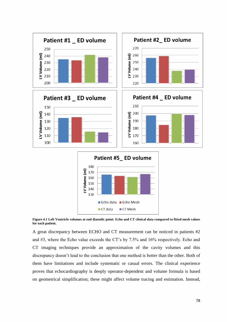
78
Figure 4.1 Left Ventricle volumes at end diastolic point: Echo and CT clinical data compared to fitted mesh values
for each patient.
A great discrepancy between ECHO and CT measurement can be noticed in patients #2
and #3, where the Echo value exceeds the CT’s by 7.5% and 16% respectively. Echo and
CT imaging techniques provide an approximation of the cavity volumes and this
discrepancy doesn’t lead to the conclusion that one method is better than the other. Both of
them have limitations and include systematic or casual errors. The clinical experience
proves that echocardiography is deeply operator-dependent and volume formula is based
on geometrical simplification; these might affect volume tracing and estimation. Instead,
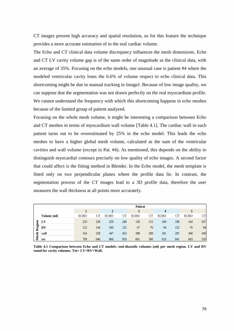
79
CT images present high accuracy and spatial resolution, so for this feature the technique
provides a more accurate estimation of to the real cardiac volume.
The Echo and CT clinical data volume discrepancy influences the mesh dimensions. Echo
and CT LV cavity volume gap is of the same order of magnitude as the clinical data, with
an average of 35%. Focusing on the echo models, one unusual case is patient #4 where the
modeled ventricular cavity loses the 6.6% of volume respect to echo clinical data. This
shortcoming might be due to manual tracking in ImageJ. Because of low image quality, we
can suppose that the segmentation was not drawn perfectly on the real myocardium profile.
We cannot understand the frequency with which this shortcoming happens in echo meshes
because of the limited group of patient analyzed.
Focusing on the whole mesh volume, it might be interesting a comparison between Echo
and CT meshes in terms of myocardium wall volume [Table 4.1]. The cardiac wall in each
patient turns out to be overestimated by 25% in the echo model. This leads the echo
meshes to have a higher global mesh volume, calculated as the sum of the ventricular
cavities and wall volume (except in Pat. #4). As mentioned, this depends on the ability to
distinguish myocardial contours precisely on low quality of echo images. A second factor
that could affect is the fitting method in Blender. In the Echo model, the mesh template is
fitted only on two perpendicular planes where the profile data lie. In contrast, the
segmentation process of the CT images lead to a 3D profile data, therefore the user
measures the wall thickness at all points more accurately.
Table 4.1 Comparison between Echo and CT models: end-diastolic volumes (ml) per mesh region. LV and RV
stand for cavity volumes. Tot= LV+RV+Wall.
1 2 3 4 5
Volume (ml) ECHO CT ECHO CT ECHO CT ECHO CT ECHO CT
LV 233 238 259 240 136 115 184 198 164 167
RV 122 144 160 125 67 76 94 152 70 94
wall 354 258 447 453 398 309 341 291 368 249
tot 709 640 866 818 601 500 619 641 603 510
Patient
Mesh
Regio
n

80
4.3. Unloaded Geometry
4.3.1. New Loaded and Unloaded Volumes Analysis
Starting from the end diastolic fitted mesh, the Krishnamurthy’s iterative algorithm is
applied with the aim to estimate the unloaded configuration. The process is iterated until
the loaded geometry (“LoadM”) and the fitted end-diastolic (“FitM”) geometry matched to
within a previously set value of tolerance. The error between the two meshes is the
difference in mm between nodes coordinates (NC), computed at each inflation step with
the following formula:
𝑅𝑒𝑙𝐸𝑟𝑟(𝑥, 𝑦, 𝑧) = |𝑁𝐶(𝑥, 𝑦, 𝑧)𝐹𝑖𝑡𝑀 − 𝑁𝐶(𝑥, 𝑦, 𝑧)𝐿𝑜𝑎𝑑𝑀|
The error was first calculated for the three coordinates X,Y,Z, followed by averaging.
Figure 4.3 shows three examples of the error trend in function of the iteration number. The
red line refers to the reference error, defined by Krishnamurthy [32].
The iteration corresponding to the lower error is the one from which the new loaded mesh
derives.

81
For patient #4, iterations #4 and #5 reveal a “steady state”.
We further evaluated the final loaded mesh LV cavity volume with a different method.
For this task, the new loaded inflated mesh was compared with the echo volume
measurement, as carried out for the fitting mesh (section 4.1). Table 4.2 summarizes the
two configurations at end diastolic point with their relative error with the echo data
measure.
The error is computed with the formula:
𝐸𝑟𝑟(%) =|𝑉𝑜𝑙(𝐴 𝑜𝑟 𝐵) − 𝑉𝑜𝑙(𝐶)|
𝑉𝑜𝑙(𝐶)∗ 100
Reference error =0.5 mm
Figure 4.2 Absolute error (mm) between fitted mesh and new loaded mesh at each iteration for patients number
1,3,4. Within three iterations it becomes lower than the reference error.

82
In Pat#4 and Pat#2 , the reduction of the error with the clinical data is respectively 30%
and 65%, improving quantitatively anatomical dimension modeling. In contrast, Patient #3
presents a higher discrepancy with the new loaded mesh. Patients # 1 and #5 are not
affected by changes. These results lead to conclude that for the echo models (CT models
results are not available), the unloading algorithm allows to error minimization raised
during the fitting process.
Table 4.2 LV volumes of “new” loaded mesh (obtained with unloading algorithm), fitted mesh and echo
measurements. The two errors stress the global decreased/increased volume loss between the computed and
clinical values.
Focusing on the estimated unloaded LV volumes between the two models [Table 4.3],
percentages of the unloaded cavity respect to the fitted volume have been evaluated for
both the models. We can infer that the echo unloaded meshes and echo fitted volumes
present the same volume ratio respect to the CT unloaded and fitted meshes. This means
that the averaging of the patient specific passive material properties didn’t lead to
meaningful alteration of the “unloading” process.
Generally the Echo and CT unloaded computed volumes match with the empirical volume
within the 10% of error [Table 4.3]. Notice that the estimated-empirical volume error is in
the same percentage between Echo and CT models. In both the analyzed indexes, patients
#2 and #4 are the exceptions.
New Loaded (A) Fitted (B)
Pat 1 233 233 235 0.85 0.85
Pat 2 255 259 256 0.39 1.17
Pat 3 133 136 135 1.48 0.74
Pat 4 188 184 197 4.57 6.60
Pat 5 164 164 166 1.20 1.20
Err (%) btw
A-C
Err (%) btw
B-CEnd Diastolic Mesh
LV VOLUME (ml)
Echo Data (C )

83
Table 4.3 Simulated and Klotz unloaded volumes for Echo and CT models.
4.3.2. Passive Inflation Analysis
The passive inflation curve of Echo and CT models are compared with the empirical
Klotz’s PV relation in Figure 4.3. In the range of pressure from 0 mmHg to the end
diastolic point, the percentage error between the simulated passive curve and the empirical
volumes is calculated and shown in Figure 4.4.
The highest error peak is generally located within the first quarter of pressure range (0-
25%) (early filling phase) for both the Echo and CT models. Considering the global error
trend, for patient #1 and 4, the Echo-Klotz error is almost constantly under the 5% and
lower than the CT-Klotz. In these two cases the averaged values used for the material
properties optimized the simulated and the empirical curve match. Pat #5 is the case where
the Echo error exceeds the CT’s. This is the case where a customization of the passive
parameters could have optimized the results.
1 2 3 4 5
ECHO CT ECHO CT ECHO CT ECHO CT ECHO CT
Simulated Unloaded (ml) 132 132 145 115 67 56 92 114 86 85
Fitting mesh 233 238 259 240 136 115 184 198 164 167
Unloaded Vol/Fitting Vol % 57 55 56 48 49 49 50 58 52 51
Klotz Unloaded (ml) 106 110 120 112 65 55 93 97 94 92
Unloaded Vol/ Klotz Vol % 20 17 17 3 3 2 1 15 9 8
Patient
LV Volume

84
Figure 4.3 Passive inflation curves of Echo and CT simulations and respective Klotz empirical curves.

85
Figure 4.4 Simulated passive inflation-Klotz curves (percentage error): Echo and CT models show the highest
error peak during the first filling phase. This is minimized to zero reaching the end diastolic pressure.

86
4.4. Full Beat Simulation and Pressure-time plot
In order to simulate a full cardiac cycle, the finite element models of the ventricles were in
a non-linear lumped parameter systems model of the systemic and pulmonary circulation
(the CircAdapt Chapter 2).
The full beat simulation firstly takes the new loaded mesh for the isovolumetric contraction
phase and consists in ten beats. Since the steady state is achieved during the tenth, the
analysis is carried out only on the last beat outcome.
The length of the contractile element (Lsi) and contractility (Con) parameters are set to
default values during the first beat. These variables, referring to each node, are updated
every beat and saved in DynamicGPT#.xls file where # is the number of the current beat.
The python script takes it as input for the following cardiac cycle. An example of updating
is shown for patient #5 in table 4.4, where the value is the mean at each beat. Notice that
there is no meaningful difference after ten beats for both the parameters.
Table 4.4 At the end of each cardiac beat the contractility and the length of contractile element values are
updated and used as inputs for the following beat.
At first, the full beat simulations were driven out with the same stress scaling factor σact
values imported from CT models. It was observed that echo simulated systolic peak did not
match accurately the clinical data. To overcome this problem, it was necessary to assess a
new σact value for some patients [Table 4.5].

87
Table 4.5 Active model parameter: stress scaling factor σact modification from CT to Echo model in order to
match the clinical data.
Figure 4.5 shows only the tenth beat for the left ventricle next to σact modification . This
study doesn’t focus on the right ventricle.
The first loop (not displayed) starts with the passive inflation’s outputs, which are the end
diastolic volume and pressure (EDV and EDP respectively). In fact in the continuity file,
the initial condition form contains the new loaded mesh and in the circulatory model the
LV and RV pressures are set to EDP . Over ten beats these two values are adapted in order
to catch the systolic peak and stroke volume. In fact in some cases (Pat 1,3) the loops are
shifted from the passive inflation curve. During the full beat simulation, the biventricular
mesh is virtually linked to a cardiopulmonary system, and when pre or post loads are
applied, telediastolic volume changes.
Paying attention to the pressure time-course over the tenth beat, simulated curve and
clinical recordings are shown in Figure 4.6. The pressure data is the average of multiple
beats and was recorded invasively using catheter. In Pat #4, the σact modification yielded
the simulated-clinical data discrepancy to decrease by the 25%.
Echo CT
Pat 1 260 220
Pat 2 150 150
Pat 3 75 75
Pat 4 50 70
Pat 5 270 150
σact (kPa)

88
Figure 4.5 Full beat simulation, including passive inflation curve both for Echo and CT model.
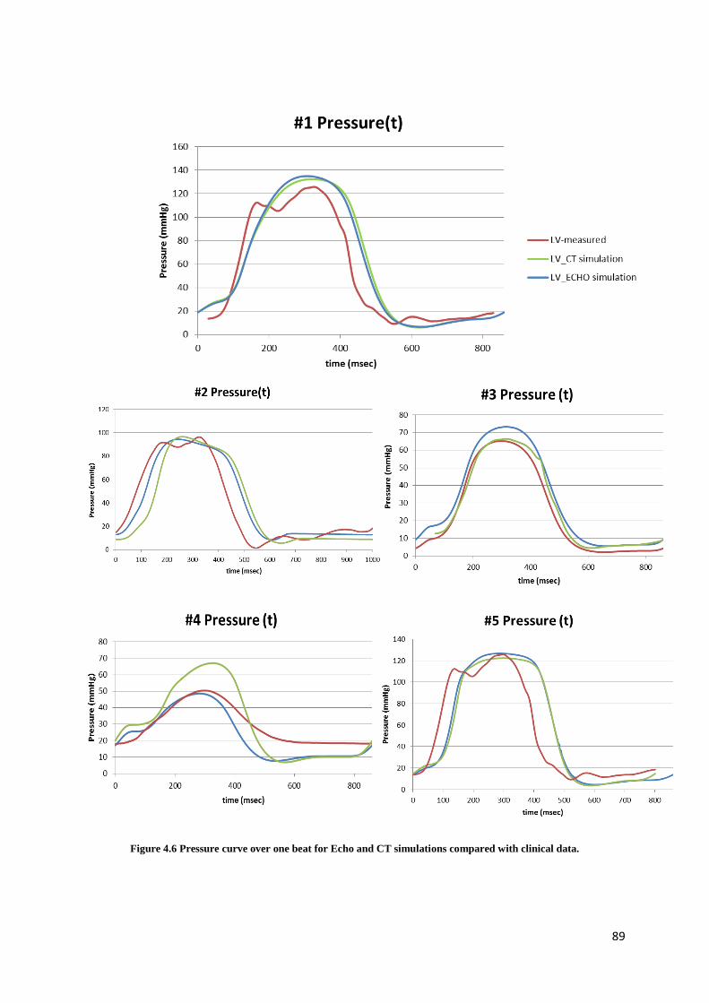
89
Figure 4.6 Pressure curve over one beat for Echo and CT simulations compared with clinical data.
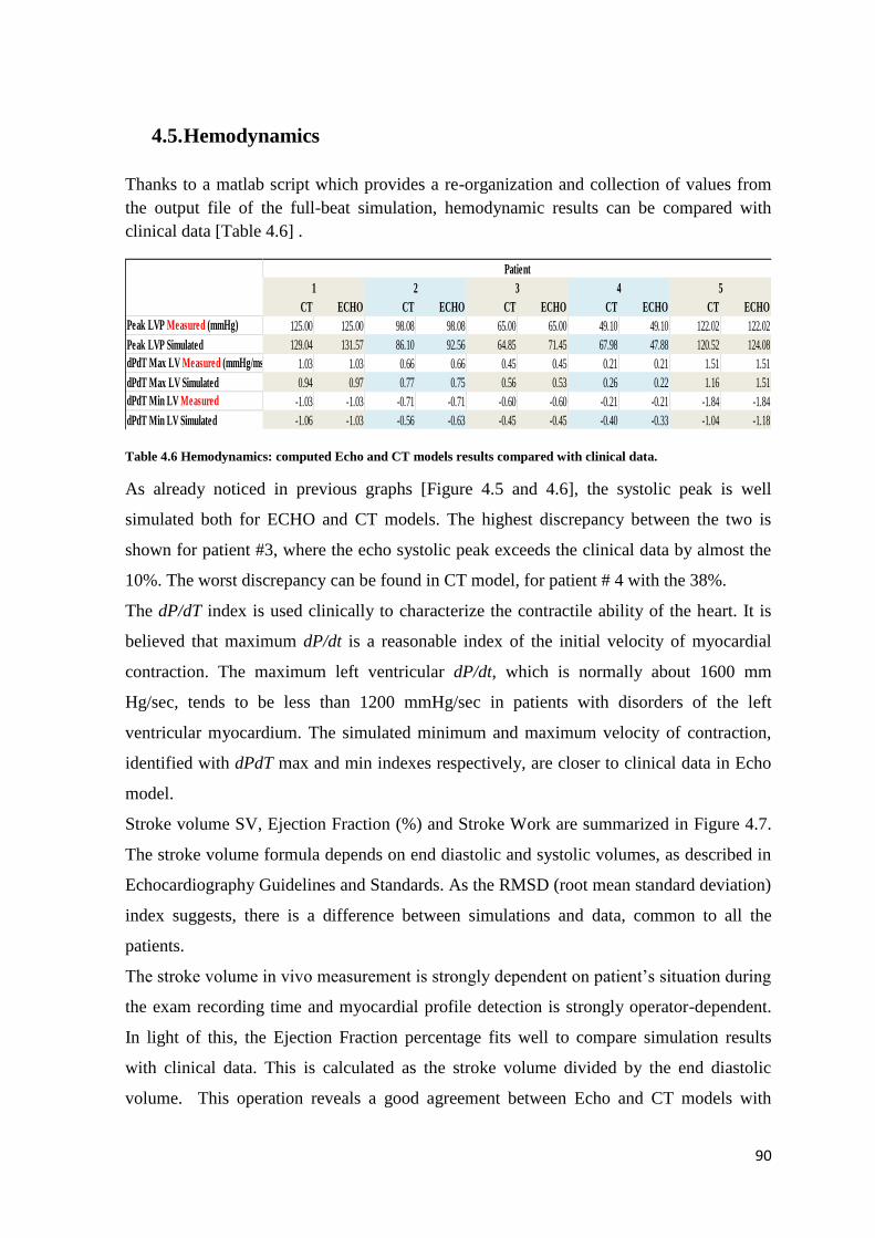
90
4.5. Hemodynamics
Thanks to a matlab script which provides a re-organization and collection of values from
the output file of the full-beat simulation, hemodynamic results can be compared with
clinical data [Table 4.6] .
Table 4.6 Hemodynamics: computed Echo and CT models results compared with clinical data.
As already noticed in previous graphs [Figure 4.5 and 4.6], the systolic peak is well
simulated both for ECHO and CT models. The highest discrepancy between the two is
shown for patient #3, where the echo systolic peak exceeds the clinical data by almost the
10%. The worst discrepancy can be found in CT model, for patient # 4 with the 38%.
The dP/dT index is used clinically to characterize the contractile ability of the heart. It is
believed that maximum dP/dt is a reasonable index of the initial velocity of myocardial
contraction. The maximum left ventricular dP/dt, which is normally about 1600 mm
Hg/sec, tends to be less than 1200 mmHg/sec in patients with disorders of the left
ventricular myocardium. The simulated minimum and maximum velocity of contraction,
identified with dPdT max and min indexes respectively, are closer to clinical data in Echo
model.
Stroke volume SV, Ejection Fraction (%) and Stroke Work are summarized in Figure 4.7.
The stroke volume formula depends on end diastolic and systolic volumes, as described in
Echocardiography Guidelines and Standards. As the RMSD (root mean standard deviation)
index suggests, there is a difference between simulations and data, common to all the
patients.
The stroke volume in vivo measurement is strongly dependent on patient’s situation during
the exam recording time and myocardial profile detection is strongly operator-dependent.
In light of this, the Ejection Fraction percentage fits well to compare simulation results
with clinical data. This is calculated as the stroke volume divided by the end diastolic
volume. This operation reveals a good agreement between Echo and CT models with
CT ECHO CT ECHO CT ECHO CT ECHO CT ECHO
Peak LVP Measured (mmHg) 125.00 125.00 98.08 98.08 65.00 65.00 49.10 49.10 122.02 122.02
Peak LVP Simulated 129.04 131.57 86.10 92.56 64.85 71.45 67.98 47.88 120.52 124.08
dPdT Max LV Measured (mmHg/ms) 1.03 1.03 0.66 0.66 0.45 0.45 0.21 0.21 1.51 1.51
dPdT Max LV Simulated 0.94 0.97 0.77 0.75 0.56 0.53 0.26 0.22 1.16 1.51
dPdT Min LV Measured -1.03 -1.03 -0.71 -0.71 -0.60 -0.60 -0.21 -0.21 -1.84 -1.84
dPdT Min LV Simulated -1.06 -1.03 -0.56 -0.63 -0.45 -0.45 -0.40 -0.33 -1.04 -1.18
Patient
1 2 3 4 5

91
clinical measurement. All the patients have a EF % less than 40%: these are pathological
results, typical for people affected by left ventricle dysfunction. Beside, EF index lower
than 35% is one among the factors for CRT patients selection.
Stroke work histogram is in line with this. For this index there is no clinical data available
for comparison. Echo prediction agrees within the 15% with the CT model.
Figure 4.7 Stroke Volume and Ejection Fraction where Echo and CT results are compared with clinical data,
RMSD and NRMSD calculated. Missing clinical data for Stoke Work
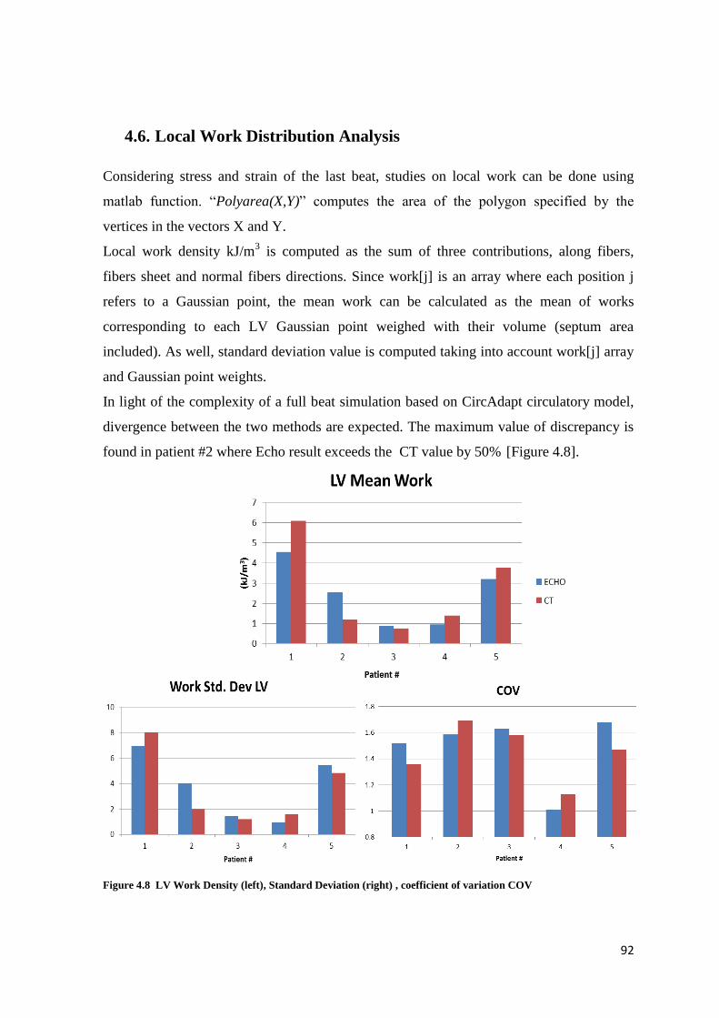
92
4.6. Local Work Distribution Analysis
Considering stress and strain of the last beat, studies on local work can be done using
matlab function. “Polyarea(X,Y)” computes the area of the polygon specified by the
vertices in the vectors X and Y.
Local work density kJ/m3 is computed as the sum of three contributions, along fibers,
fibers sheet and normal fibers directions. Since work[j] is an array where each position j
refers to a Gaussian point, the mean work can be calculated as the mean of works
corresponding to each LV Gaussian point weighed with their volume (septum area
included). As well, standard deviation value is computed taking into account work[j] array
and Gaussian point weights.
In light of the complexity of a full beat simulation based on CircAdapt circulatory model,
divergence between the two methods are expected. The maximum value of discrepancy is
found in patient #2 where Echo result exceeds the CT value by 50% [Figure 4.8].
Figure 4.8 LV Work Density (left), Standard Deviation (right) , coefficient of variation COV
93
The standard deviation (SD) suggests a great dispersion of local work for all the patients.
Coefficient of variation, that is the SD value divided by the work density mean, reflects the
deep data dispersion. This leads to conclude that the work distribution is not homogeneous
on the cardiac wall. A further investigation has been run to find a correspondence between
activation time pattern/scar region and work density distribution.
Figures 4.9 and 4.10 show work distribution analysis for two patients, as sample: Patient
#3 and Patient #2 with scar region. Each plot has on the X axis the Gaussian points, 27 per
each element of the mesh, for a total amount of 3456. These are grouped in colored boxes
depending on the mesh region they belong to. Myocardial sectors are shown in the 3D
views.
The LV mean work density is calculated on the 81% of mesh elements. These LV
elements are distributed from the apex to the base of the mesh and are supposed to act
differently during the cardiac beat. This is demonstrated in the Work Density plot in Figure
4.9 (red box): LV Gaussian points which correspond to the higher work peaks are located
at the base of the mesh. This can explain the high SD values shown in Figure 4.8.
Considering the entire biventricular mesh, work density distribution can be correlated also
with infarcted regions and activation time. The medium-late activated regions carry out
the highest contribution of work density. Besides, they refer to the left
ventricular/septal/epicardial sectors at the base of the finite element mesh.
Figure 4.10 displays results for Patient #5 in line with these considerations. The scar region
plot presents a red borderline which separates the infarcted and non-infarcted Gaussian
points (respectively above and below 0.6). The higher the infarction value is, the more
depressed is the local work carried out. The most important contribution of work density is
provided by non-infarcted regions at the base of the 3D model, as in the previous case.
Accordingly, the medium late activated elements in the left ventricle section perform a
great amount of work. The work density lowers in apex regions, which beside correspond
to elevated scar tissue values, in line with biological behavior.
The work density distribution cannot be compared with CT model because of lacking of
results. However, in literature different studies have reported a similar distribution for
biventricular meshes [60]. This work distribution is a feature for patients affected by
LBBB dyssynchrony. The RV apex pacing leads the late activated regions to perform
higher work, i.e. LV base.

94
Figure 4.9 Patient #6 work distribution, activation time pattern plots on the top. The colored sections correspond
to specific myocardial region as shown in the legend. 3D mesh on the right with highlighted regions.
Left ventricle+Septum
Apex
Epicardium
Right ventricle
Top view Inferior view

95

96
Figure 4.10 Patient #5 Scar region distribution shows a good agreement with work density distribution. Where the
scar value is above the red borderline (0.6) the region is considered infarcted.
Left ventricle+Septum
Apex
Epicardium
Right ventricle
Top-view Inferior-view

97
5. CONCLUSIONS AND FUTURE DEVELOPMENTS
98
5.1. CONCLUSIONS
This project was entirely developed at UCSD, University of California San Diego
Bioengineering Department CMRG (Cardiac Mechanic Research Group) Lab under the
supervision of Andrew McCulloch.
The aim of this study was to investigate the feasibility of using echocardiography derived
meshes for patient-specific (PS) cardiac models as a replacement of the gold standard CT
for a future employment of computational modeling on a large scale.
To this end, using a semi-automated workflow as described in the material and methods
section, biventricular meshes of five patients with ventricular dysfunction were constructed
from 2D ultrasounds images. These models were then used for simulation and analysis of the
cardiac mechanics. The presented model is compared to a previous study (“CT model”),
which developed cardiac biomechanical models for the same cohort of patient making use
of CT images for the biventricular geometry.
The implemented method for the mesh creation from Echo images, based on both manual
and automatic fitting, led to obtain cavity volumes consistent with the echo clinical data.
The volume discrepancy between the Echo and CT fitted meshes is mainly due to the
difference between Echo and CT volume valuation. This was expected considering the
higher resolution on CT compared to echocardiography.
Apart from the volumetric analysis, the Echo model results are in good accordance with
the CT’s. For example, the Echo and CT unloaded geometries estimated through an
iterative algorithm show the equivalent percentage of error compared to the empirical
Klotz’s unloaded volume. The Echo simulated passive inflation curves in some cases
matched the empirical Klotz’s curve with an error 5% lower than CT’s.
Furthermore, hemodynamic outcome shows a good agreement between computed values
and clinical data. LV Ejection fraction and the velocity of contraction indexes (dP/dt)
simulated by the Echo models present the same accuracy of the CT values. In light of these
results, we may notice that the Echo and CT models are both capable of replicating patient-
specific global cardiac function.
The last work analysis provided an outcome consistent with left ventricle dysfunction’s
effect. In fact, the work density is deeply concerned with the activation pattern and
infarcted areas. For the patient analyzed, the highest work contribution is localized on the
left ventricle epicardial anterior wall, while the apex is characterized by zero level of work.
99
Besides, scar regions are characterized by a cardiac work close to zero or even negative. In
this terms, the echo models also simulated a work distribution already confirmed by
previous study in literature [60].
The outcome presented in chapter 4 makes the model consistent and acceptable through a
clinical data comparison. This leads to the conclusion that Echo imaging could be a
potential driver of progress for a future development of cardiac models on large scale.
However, significant improvements should be realized before the echo meshes will truly
be able to approximate the ventricular geometry within the same accuracy of CT technique.
5.2. FUTURE DEVELOPMENTS
During the project development, the following limitations have been identified:
Mesh segmentation and fitting steps: we noticed that the number of echo images used
were not enough to accurately model the anatomical detail.
Patient specific values: the mathematical models require a robust amount of patient
specific parameters, whose definition is based on invasive clinical exams. This aspect
enters in contrast with the project’s aim to use low-cost techniques.
Results comparison: a more accurate dimension analysis could have been carried out,
considering Echo mesh ventricular shape and contours compared to the CT meshes.
Using an averaged group of material properties probably led to increase the
discrepancy between simulated passive curve and full beat results. The next step could
use the original patient-specific properties in order to investigate if this improves the
results.
In light of these aspects, the next steps towards the translation of this technology into
clinical environments regards the improvement of the model-building procedures.
First, the realization of a more accurate geometry with a lower loss of anatomical details
could be realized with the use of more than two imaging planes or even with the use of 3D
echo imaging.
The echo profile tracing step might be speeded up by implementing an algorithm for
automatic detection, making it less user-dependent. From a biomechanical point of view,
patient specific parameters should be derived where possible from non-invasive clinical

100
measurements in order to simplify the cardiovascular model and to relieve patient’s
burden.
A further innovative aspect might be the implementation of a complete electromechanical
patient-specific model. Considering the pathological condition of the analyzed patients, the
incorporation of the electrical model would be interesting for a more detailed investigation.
Even if this research field has a substantial room for improvement, this project shows
promising outcome that lead to believe in a future application of echocardiography as the
low-cost clinical-routine tool to supply the required geometric data for cardiac mesh
construction.

101
6. APPENDIX

102
6.1. Constitutive model
6.1.1. Essential elements of Continuum mechanics
Kinematical quantities and invariants
The basic deformation variable for the description of the local kinematics is the
deformation gradient F, with the standard notation and convention:
𝐽 = det(𝑭) > 0 (1)
For an incompressible material, we have the constraint
𝐽 = det(𝑭) = 1 (2)
Associated with F are the right and left Cauchy–Green tensors, defined by
𝑪 = 𝑭𝑻𝑭 and 𝑩 = 𝑭𝑭𝑻 (3)
respectively. Also important for what follows is the Green–Lagrange (or Green) strain
tensor, defined by
𝑬 =1
2(𝑪 − 𝑰) (4)
where I is the identity tensor. The principal invariants of C (and also of B) are defined by
𝑰𝟏 = 𝑡𝑟(𝑪) 𝑰𝟐 =1
2[(𝑰𝟏
2 − 𝑡𝑟(𝑪𝟐)] 𝑎𝑛𝑑 𝑰𝟑 = det (𝑪) (5)
with I3 =J 2 =1 for an incompressible material. These are isotropic invariants.
If the myocardium has a preferred direction along the fiber in the reference configuration,
denoted by the unit vector f0, this introduces anisotropy, specifically transverse isotropy,
and with it come two additional (transversely isotropic) invariants defined by:
𝑰𝟒 = 𝑓0(𝑪𝑓0) 𝑎𝑛𝑑 𝑰𝟓 = 𝑓0(𝑪𝟐𝑓0) (6)
If there are two preferred directions, the second denoted by s0 (Fiber-Sheet), then this
introduces the invariants:
𝑰𝟔 = 𝑠0(𝑪𝑠0) 𝑎𝑛𝑑 𝑰𝟕 = 𝑠0(𝑪𝟐𝑠0) (7)
associated with it and, additionally, a coupling invariant, denoted by I8, which is defined as
follows:
𝑰𝟖 = 𝑓0(𝑪𝑠0) = 𝑠0(𝑪𝑓0) (8)

103
Strain-energy function and stress tensors
The material properties are described by a strain-energy function Ψ, which is measured per
unit reference volume. This depends on the deformation gradient F through C
(equivalently through E), which ensures objectivity. For such an elastic material, the
Cauchy stress tensor σ is given by the formulae:
𝐽𝛔 = 𝐅𝛿𝚿
𝛿𝑭= 𝐅
𝛿𝚿
𝛿𝑬𝑭𝑻 (9a)
for a compressible material (for Ψ treated as a function of F and E, respectively),
which are modified to:
𝝈 = 𝑭𝛿𝜳
𝛿𝑭− 𝑝𝑰 = 𝑭
𝛿𝜳
𝛿𝑬𝑭𝑻 − 𝑝𝑰 (9b)
for an incompressible material, in which case we have the constraint J =1 (equivalently I3
=J 2 =1) and this is accommodated in the expression for the stress by the Lagrange
multiplier p.
For an elastic material possessing a strain-energy function Ψ that depends on a list of
invariants, say I1, I2, . . . , IN for some N, the equation 9a and 9b turn out to be:
𝐽𝛔 = 𝐅 ∑ Ψ𝑖 𝛿𝐼𝑖
𝛿𝑭
𝑁𝑖 𝑎𝑛𝑑 𝛔 = 𝐅 ∑ Ψ𝑖
𝛿𝐼𝑖
𝛿𝑭
𝑁𝑖=1,𝑖 ≠3
− 𝑝𝑰 (10)
Where the following notation is introduced (with i = 3 omitted from the summation for the
incompressible material):
Ψ𝑖 =𝛿𝚿
𝛿I𝑖 𝑖 = 1,2 … … 𝑁
The second Piola–Kirchhoff stress tensor S is given in terms of the Cauchy stress tensor
via the simple formula:
𝑺 = 𝐽𝑭−𝟏𝛔𝑭−𝑻
using equation (9a) for a compressible material and using equation (9b) for an
incompressible material with J =1. Explicitly, with E as the independent variable, simply
results for compressible and incompressible materials, respectively:
𝑺 =𝛿𝚿
𝛿𝑬 𝑎𝑛𝑑 𝑺 =
𝛿𝚿
𝛿𝑬− 𝑝(𝑰 + 2𝑬)−1 (11)
Transversely Isotropic Slightly Compressible material
Under the assumption of isotropy, the strain energy function depends only on the left (or
right) Cauchy-Green tensor through the invariants I,II,III.

104
In the compressible case all invariants are independent and no constraint exists. In this case
a totally decoupled isochoric and volumetric material behavior is commonly assumed and
the strain function results split in:
Ψ = Ψ𝑖𝑠𝑜(𝐼) + Ψ𝑣𝑜𝑙(𝐽)
In this study myocardium tissue is considered a slightly compressible material, for the
isochoric component the strain energy refers to Ogden-Holzapfel model and for the
volumetric is used a newly proposed function.
The isochoric strain function is expressed as exponential function end depends on eight
parameters.
Ψiso = 𝑎
2𝑏𝑒𝑏(𝐼1−3) + ∑
𝑎𝑖
2𝑏𝑖{𝑒𝑏𝑖(𝐼4𝑖−1)2
− 1} +𝑎𝑓𝑠
2𝑏𝑓𝑠[𝑒𝑏𝑓𝑠𝐼8𝑓𝑠
2− 1]𝑖=𝑓,𝑠 (12)
where a, b, af, as, bf , bs, afs and bfs are eight positive material constants, the a parameters
having dimension of stress, whereas the b parameters are dimensionless [9].
The volumetric part Ψvol(J) comes from the following equation:
𝚿vol(J) = K(J − 1) ∗ ln(𝐽) /2 (13)
Parameters used in this study are listed in table 6.1.
The second Piola Kirchhoff stress tensor Spass derived from these two strain functions
refers to the passive component of the mechanical behavior. In order to compute the total
second Piola Kirchhoff stress tensor Stot active model has to be introduced.
Parameter and unit Value
a [kPa] 0.77
b [-] 9.23
af [kPa] 0.57
bf [-] 14.98
asheet [kPa] 0.0
bsheet [-] 11.17
afs [kPa] 0.0
bfs [-] 9.46
Bulk modulus [kPa] 350
Table 6.1 Constitutive model parameters: values used.

105
6.2. Active Model
The generation of active stress in the fiber direction is calculated by the Arts model of
sarcomere mechanics [51], in which the length of the contractile element (Lsc) and a time-
variant contractility parameter (C) were state variables. The normalized length of the series
elastic element (LsNorm) was calculated by:
LsNorm = (Ls- Lsc)/LSerEl (14)
where Ls is sarcomere length and LSerEl length of the series elastic element during isometric
contraction. The contractile element velocity (dLsc/dt) is calculated by:
(15)
This contractile element velocity is a modification from Lumens et al(6), which yields a
hyperbolic Hill-relation between shortening velocity and force.
Contractility C is obtained having separate terms to describe rise and decay of mechanical
activation C:
(16)
where
t is time elapsed since electrical activation (*);
CL tanh(2 (Lsc Ls0)2) (17)
regulates contractility dependence on contractile element length;
frise 0.02(8 x)2x3ex (18)
with x=min(8,max(0,t/r)) regulates rise of contractility and
(19)
regulates twitch duration as function of contractile element length. Parameters r and d
are scaling rise and decay time, respectively [Table 2].
Active fiber stress f,a is calculated by
f ,a act C LsNorm (20)
Equation 20 is a modification from [51,40] such that active tension does not increase
indefinitely with increasing sarcomere length. This imposes a limit on the total amount of
work a fiber can generate. Active stress is also generated transverse to the myofibers, and
dLsc
dt
LsNorm -1
bhill LsNorm +1vmax LsNorm 1
LsNorm -1
bHill LsNorm +1vmax e
aHill (LsNorm1) LsNorm 1
dC
dt1
r CL f rise
1
dCrest C
1 e(T t )/d
T sc(0.290.3Lsc)

106
was about 40% of active stress generated in the myofiber direction [41]. Table 6.2 lists the
values of the contractile material parameters.
From σf,a, the three main direction components of the active tensor can be calculated:
𝑡𝑠𝑠 = 𝑎𝑙𝑝ℎ𝑎2 ∗ 𝜎𝑓, 𝑎 (21)
𝑡𝑛𝑛 = 𝑎𝑙𝑝ℎ𝑎3 ∗ 𝜎𝑓, 𝑎
𝑡𝑓𝑓 = 𝜎𝑓, 𝑎/𝑠𝑞𝑟𝑡(𝐶[0,0])
Where s is the fiber sheet direction, n is normal to the fiber sheet, and f is along the fiber
and alpha2 and alpha3 are constants defined by users [Table 6.2].
Then, in order to get the Active 1st Piola-Kirchoff Stress Tensor Sact:
𝑡𝑐11 = 0.5 ∗ (2.0 − alphas − alphan) ∗ tff + ((0.25 +1.0
2.0∗pi) ∗ alphas + (0.25 −
1.0
2.0∗pi) ∗ alphan) ∗
tss + ((0.25 −1.0
2.0∗pi) ∗ alphas + (0.25 +
1.0
2.0∗pi) ∗ alphan) ∗ tnn (22)
𝑡𝑐22 = 0.5 ∗ (2.0 − alphas − alphan) ∗ tss ∗ (sqrt(C[1,1])
sqrt(C[0,0])) + ((0.25 +
1.0
2.0∗pi) ∗ alphas + (0.25 −
1.0
2.0∗pi) ∗
alphan) ∗ (tff + tnn) ∗ (sqrt(C[1,1])
sqrt(C[0,0])) (23)
𝑡𝑐33 = 0.5 ∗ (2.0 − 𝑎𝑙𝑝ℎ𝑎𝑠 − 𝑎𝑙𝑝ℎ𝑎𝑛) ∗ 𝑡𝑛𝑛 ∗ (𝑠𝑞𝑟𝑡(𝐶[2,2])
𝑠𝑞𝑟𝑡(𝐶[0,0])) + ((0.25 −
1.0
2.0∗𝑝𝑖) ∗ 𝑎𝑙𝑝ℎ𝑎𝑠 + (0.25 +
1.0
2.0∗𝑝𝑖) ∗ 𝑎𝑙𝑝ℎ𝑎𝑛) ∗ (𝑡𝑓𝑓 + 𝑡𝑠𝑠) ∗ (
𝑠𝑞𝑟𝑡(𝐶[2,2])
𝑠𝑞𝑟𝑡(𝐶[0,0])) (24)
Finally:
𝑺𝒂𝒄𝒕 = 𝑀𝑎𝑡𝑟𝑖𝑥([[𝑡𝑐11,0,0], [0, 𝑡𝑐22,0], [0,0, 𝑡𝑐33]]) (25)
As previously anticipated, the passive and active components have to be summed to obtain
the total second Piola Kirchhoff stress tensor 𝑆𝑡𝑜𝑡 = 𝑆𝑝𝑎𝑠𝑠 + 𝑆𝑎𝑐𝑡.
Parameter and unit Description Value
aHill [-] Parameter that determines curvature of Hill relation during stretching 1.5
Crest [-] Diastolic contractility level 0.0
bHill [-] Parameter that determines curvature of Hill relation during shortening 1.5
Ls0 [m] Contractile element length at zero active stress 1.51
LSerEl [m] Length of series elastic element during isometric contraction 0.04
vmax [m/sec] Sarcomere shortening velocity with zero load 7.0
d [ms] Relaxation time scaling factor 15
r [ms] Contraction rise time scaling factor 28.1
sc [ms] Twitch duration scaling factor 293
act [kPa] Active stress scaling factor (default value, in this project is Patient Specific) 65.0

107
alpha2 constant 0.3
alpha3 constant 0.3
alpha_n constant 0.152
alpha_s constant 0.152
Table 6.2 Active material properties of the mechanics model.
(*) Computationally, t is a local time calculated as:
𝑡𝑙𝑜𝑐𝑎𝑙 = {𝑀𝑜𝑑(𝑡 − 𝑡𝑎𝑐𝑡 , 𝑏𝑙𝑐) 𝑡 > 𝑡_𝑎𝑐𝑡𝑖𝑣𝑒(𝑡 − 𝑡𝑎𝑐𝑡) 𝑡 ≤ 𝑡_𝑎𝑐𝑡𝑖𝑣𝑒
Where tact is node-specific value in the mesh and blc is the beat cycle length. The patients
analyzed have a blc set to 860 msec, except Patient #2 with a blc set to 1000 msec.
6.3. Circulatory Model Parameters
Despite the previous paragraphs, this section is used to provide the group of Patient
Specific parameters imported from Krishnamurthy’s model [32] [Table 6.3]. We refer to
the literature for detailed analysis of the CircAdapt model [50].
Parameter description and unit Value
Blood density [kg/liter] 1.05
Average cardiac output setpoint [liter/min] 1.8
Left and right atrium
atrial-ventricular activation delay time [ms] 120
atrial inflow lumen area [cm2] 3.6
atrial inflow lumen length [cm] 1.26
atrial reference midwall area [cm2] 46.5
atrial dead midwall area [cm2] 8.0
left atrial wall volume [cm3] 7.45
right atrial wall volume [cm3] 1.87
atrial length series elastic element [m] 0.04
atrial contraction rise time factor [ms] 45
atrial relaxation time factor [ms] 30
atrial twitch duration [ms] 200
atrial sarcomere length when active stress is zero [m] 1.51
atrial sarcomere length when passive stress is zero [m] 1.8
atrial sarcomere compliance factor [m/kPa] 0.8
atrial passive fiber stress scaling factor [kPa] 23.7
atrial resting contractility [-] 0.02
atrial sarcomere reference length [m] 2.0
atrial active fiber stress scaling factor [kPa] 84.0
atrial unloaded sarcomere shortening velocity [m/s] 10
Ventricular valves

108
mitral valve lumen area when open [cm2] 4.76
mitral valve lumen area when closed [cm2] Normal and aortic stenosis: 510
-6
Mitral regurgitation: 0.35
mitral valve orifice length [cm] 0.79
aortic valve lumen area when open [cm2] Normal and mitral regurgitation:
2.7
Aortic stenosis: 0.15
aortic valve lumen area when closed [cm2] 210
-6
aortic valve orifice length [cm] 0.72
tricuspid valve lumen area when open [cm2] 4.76
tricuspid valve lumen area when closed [cm2] 510
-6
tricuspid valve orifice length [cm] 0.79
pulmonary valve lumen area when open [cm2] 2.1
pulmonary valve lumen area when closed [cm2] 210
-6
pulmonary artery orifice length [cm] 0.72
Aorta
wall cross-sectional area [cm2] 0.99
unloaded lumen area [cm2] 2.7
length of aorta [cm] 25.2
reference pressure [kPa] 12.3
wall stress power scaling factor [-] 1.7
Vena Cava
wall cross-sectional area [cm2] 0.13
unloaded lumen area [cm2] 2.5
length of vena cava [cm] 25.2
reference pressure [kPa] 0.34
wall stress power scaling factor [-] 2.3
Pulmonary artery
wall cross-sectional area [cm2] 0.23
unloaded lumen area [cm2] 2.02
length of pulmonary artery [cm] 12.6
reference pressure [kPa] 2.4
wall stress power scaling factor [-] 1.7
Pulmonary vein
wall cross-sectional area [cm2] 0.2
unloaded lumen area [cm2] 2.0
length of pulmonary vein [cm] 12.6
reference pressure [kPa] 0.94
wall stress power scaling factor [-] 2.3
pulmonary drop pressure [kPa] 1.5
Initial Condition Value
time [s] 0.0
left ventricular pressure [kPa] 1.1
right ventricular pressure [kPa] 0.2
left atrial volume [ml] 27.4
aortic volume [ml] 59.1
vena cava volume [ml] 54.8
right atrial volume [ml] 35.8
pulmonary artery volume [ml] 20.4
pulmonary vein volume [ml] 26.7
aortic valve flow [liter/s] 0
mitral valve flow [liter/s] 0.09
pulmonary artery valve flow [liter/s] 0
tricuspid valve flow [liter/s] 0.15
flow into left atrium [liter/s] -0.03
flow into right atrium [liter/s] -0.03
left atrial contractility [-] 0.83

109
left atrial contractile element length [m] 1.82
right atrial contractility [-] 0.97
right atrial contractile element length [m] 1.95
Table 6.3 CircAdapt model: list of patient-specific parameters used in this project.

110
7. REFERENCES
1. M. Neal, R. Kerckhoffs “Current progress in patient-specific modeling” 2009;
2. Chun G. Schiros “Biventricular Active Mesh Model of the Heart and Analysis of
Morphologic Changes Toward Physiology and Pathologies” 2012;
3. Alejandro Lopez-Perez, Rafael Sebastian and Jose M Ferrero “Three-dimensional
cardiac computational modelling: methods, features and applications” 2015;
4. C. Sprouse, A. Jorstad, D. DeMenthon, P. Burlina, F. Contijoch, “Computational
Cardiac Modeling Based on Transesophageal Echocardiographic Imaging” 2010;
5. P. Lamata, R. Casero, V. Carapella “Images as drivers of progress in cardiac
computational modelling” 2014;
6. A. Palit, S. Bhudia, T. N. Arvanitis “Computational modelling of left-ventricular
diastolic mechanics: Effect of fibre orientation and right-ventricle topology” 2014;
7. Streeter, D.D., Jr. “Gross morphology and fiber geometry of the heart, in Handbook of
Physiology” ;
8. C. P. Fleming, Crystal M. R., B. Webb, I. R. Efimov, A. M. Rollins “Quantification of
cardiac fiber orientation using optical coherence tomography” 2008;
9. Gerhard a. Holzapfel, R. W. Ogden “Constitutive modelling of passive myocardium: a
structurally based framework for material characterization” 2009;
10. Jeroen J. Bax, Gerardo Ansalone, Ole A. Breithardt “Echocardiographic Evaluation
of Cardiac Resynchronization Therapy: Ready for Routine Clinical Use? A Critical
Appraisal” 2004 ;
11. Nelson GS, Berger RD, Fetics BJ, et al. “Left ventricular or biventricular pacing
improves cardiac function at diminished energy cost in patients with dilated
cardiomyopathy and left bundle-branch block” 2000;
12. Silke Isabelle Trautmann, Michael Kloss and Angelo Auricchio, “Cardiac
Resynchronization Therapy” 2002;
13. John Gorcsan III, Theodore Abraham, Deborah A. Agler, Jeroen J. Bax
“Echocardiography for Cardiac Resynchronization Therapy: Recommendations for
Performance and Reporting–A Report from the American Society of
Echocardiography Dyssynchrony Writing Group Endorsed by the Heart Rhythm
Society” 2008;
111
14. Cazeau S, Leclercq C, Lavergne T, et al. “Effects of multisite biventricular pacing in
patients with heart failure and intraventricular conduction delay” 2001;
15. Abraham WT, Fisher WG, Smith AL, et al. “Cardiac resynchronization in chronic
heart failure” 2002;
16. Harvey Feigenbaum, “Evolution of Echocardiography” 1996 ;
17. Victor Mor-Avi, Roberto M. Lang “Current and Evolving Echocardiographic
Techniques for the Quantitative Evaluation of Cardiac Mechanics” 2011;
18. Ashley EA, Niebauer J. “Understanding the echocardiogram” (“Cardiology
Explained”, Chapter 4) 2004;
19. Marvin A. Konstam, Daniel G. Kramer, Ayan R. Patel, Martin S. Maron, James E.
Udelson, J Am Coll, “Left Ventricular Remodeling in Heart Failure Current Concepts
in Clinical Significance and Assessment” 2011;
20. Roberto M. Lang, Luigi P. Badano, Victor Mor-Avi, et al. “Recommendations for
Cardiac Chamber Quantification by Echocardiography in Adults: An Update from the
American Society of Echocardiography and the European Association of
Cardiovascular Imaging” 2015;
21. D. Deng, P. Jiao, X. Ye, and L. Xia “An Image-Based Model of the Whole Human
Heart with Detailed Anatomical Structure and Fiber Orientation” 2012;
22. Crozier, M. Augustin, Neic,J. Prassl, Holler, E. Fastl, Hennemuth “Image-Based
Personalization of Cardiac Anatomy for Coupled Electromechanical Modeling” 2015.
23. Herman L. Falsetti, Robert E. Mates, Colin Grant, David G. Greene, “Left Ventricular
Wall Stress Calculated from One-Plane Cineangiography” 1970;
24. Harold Sandler, Harold T. Dodge “Left Ventricular Tension and Stress in Man” 1963;
25. Vetter FJ, McCulloch AD. “Three-dimensional analysis of regional cardiac function: a
model of rabbit ventricular anatomy” 1998;
26. Nielsen PMF, Le Grice IJ, Smaill BH, Hunter PJ “Mathematical model of geometry
and fibrous structure of the heart” 1991;
27. R. M. Huisman, P. Sipkema, N. Westerhof, G. Elzinga “Comparison of models used to
calculate left ventricular wall force” 1980;
28. Frank C.P. Yin, Robert K. Strumpf, Paul H. Chew, Scott L. Zeger “Quantification of
the mechanical properties of noncontracting canine myocardium under simultaneous
biaxial loading” 1985;
112
29. Streeter, D.D.,Jr., and D.L.Bassett “An engineeering analysis of myocardial fiber
orientation in pig’s left ventricle in systole” 1966;
30. Farshad Dorri “A finite element model of the human left ventricular systole, taking into
account the fiber orientation pattern” 2004;
31. Jazmin Aguado-Sierra, Adarsh Krishnamurthy, Christopher Villongco, Andrew
McCulloch “Patient-specific modeling of dyssynchronous heart failure: A case study”
2011 ;
32. Adarsh Krishnamurthy, Christopher T. Villongco, Joyce Chuang , Andrew McCulloch
“Patient-specific models of cardiac biomechanics” 2012;
33. Christopher T. Villongco, David E. Krummen, Paul Stark, Jeffrey H. Omens, Andrew
D. McCulloch “Patient-specific modeling of ventricular activation pattern using
surface ECG-derived vectorcardiogram in bundle branch block” 2014;
34. I. J. LeGrice, B. H. Smaill, L. Z. Chai, S. G. Edgar “Laminar structure of the heart:
ventricular myocyte arrangement and connective tissue architecture in the dog” 1995;
35. P.J. Huntera, A.D. McCullochb, H.E.D.J. ter Keursc “Modelling the mechanical
properties of cardiac muscle” 1998;
36. Helm, P.A., Younes, L., Beg, M.F “Evidence of structural remodeling in
dyssynchronous failing heart” 2006;
37. Sermesant, Billet, Chabiniok, “Personalized electromechanical model of the heart for
the prediction of the acute effect of cardiac resynchronization therapy” 2009;
38. Arsigny et al. “A Log-Euclidean Framework for Statistics on Diffeomorphisms” 2006;
39. Bayer JD, Blake RC, Plank G et al. “A novel rule-based algorithm for assigning
myocardial fiber orientation to computational” 2012;
40. Wong J, Kuhl E “Generating fibre orientation maps in human heart models using
Poisson interpolation” 2012;
41. A. Palit, S. K. Bhudia, G. A. Turley “Assigning myocardial fiber orientation to a
computational biventricular human heart model” 2014;
42. A. Krishnamurthy, C. Villongco, A. Beck, J. Omens, A. McCulloch “Left Ventricular
Diastolic and Systolic Material Property Estimation from Image Data” 2015;
43. Wang, H.M., Luo, X.Y., Gao, H., Ogden, R.W., Griffith, B.E., Berry,C.,Wang,T.J., “ A
modified Holzapfel–Ogden Law for a residually stressed finite strain model of the
human left ventricle in diastole” 2014;

113
44. Walker, J.C.,Ratcliffe, M.B., Zhang,P. et al. “MRI-based finite-element analysis of left
ventricular aneurysm” 2005;
45. Sermesant, M., Razavi, R. “Personalized computational models of the heart for
cardiac resynchronization theraphy” 2010;
46. S. Klotz, I. Hay, M. L. Dickstein “Single-beat estimation of end-diastolic pressure-
volume relationship: a novel method with potential for noninvasive application” 2005;
47. N. A.Trayanova, J. J. Rice “Cardiac electromechanical models: from cell to organ”
2011;
48. Roy c. P. Kerckhoffs, S. Healy, T. Usyk, A. D. McCulloch “Computational Methods
for Cardiac Electromechanics” 2006;
49. T. Arts, J. Lumens, W. Kroon “Patient-Specific Modeling of Cardiovascular Dynamics
with a Major Role for Adaptation” 2010;
50. T. Arts, T. Delhaas, P. Bovendeerd, X. Verbeek, F. W. Prinzen “Adaptation to
mechanical load determines shape and properties of heart and circulation: the
CircAdapt model” 2004;
51. J. Lumens,t. Delhaas, b. Kirn, t. Arts “Three-Wall Segment (TriSeg) Model Describing
Mechanics and Hemodynamics of Ventricular Interaction” 2009;
52. Jason Constantino, Yuxuan Hu, Albert C. Lardo, Natalia A. Trayanova “Mechanistic
insight into prolonged electromechanical delay in dyssynchronous heart failure: a
computational study” 2013;
53. Mark Potse, Dorian Krause, Ljuba Bacharova “Similarities and differences between
electrocardiogram signs of left bundle-branch block and left-ventricular uncoupling”
2012 ;
54. Shanu B. Gupta, Mark B. Ratcliffe, Michael A. Fallert “Changes in Passive
Mechanical Stiffness of Myocardial Tissue With Aneurysm Formation” 1994;
55. Bishop MJ, Hales P, Plank G “Comparison of rule-based and DTMRI-derived fibre
architecture in a whole rat ventricular computational model” 2009;
56. S. Doll, Karl Schweizerhof “On the Development of Volumetric Strain Energy
Functions” 2000;
57. Kerckhoffs RCP, Omens JH, McCulloch AD, and Mulligan LJ “Ventricular dilation
and electrical dyssynchrony synergistically increase regional mechanical non-
uniformity but not mechanical dyssynchrony: A computational model” 2010;

114
58. Lin DHS and Yin FCP “A multiaxial constitutive law for mammalian left ventricular
myocardium in steady-state barium contracture or tetanus” 1998;
59. Costa, K.D., Holmes, J.W., McCulloch, A.D. “Modelling cardiac mechanical
properties in three dimensions” 2001;
60. Marieke Pluijmert, J. Lumens, M. Potse, T. Delhaas, Angelo Auricchio and Frits W
Prinzen “Computer Modelling for Better Diagnosis and Therapy of Patients by
Cardiac Resynchronisation Therapy” 2015;
61. J.Lumens, S. Ploux, M. Strik, MD, J. Gorcsan, et al. “Comparative electromechanical
and hemodynamic effects of left ventricular and biventricular pacing in
dyssynchronous heart failure: electrical resynchronization versus left-right ventricular
interaction” 2013;
62. S.Niederer , P. Lamata, G. Plank “Analysis of the Redistribution of Work following
Cardiac Resynchronisation Therapy in a Patient Specific Model” 2012;
63. H. Lombaert, J. Peyrat, P. Croisille “Statistical analysis of the human cardiac fiber
architecture from DT-MRI, Functional Imaging and Modeling of the Heart” 2011;
64. Roy C.P. Kerckhoffs, Jeffrey H. Omens , Andrew D. McCulloch “A single strain-
based growth law predicts concentric and eccentric cardiac growth during pressure
and volume overload” 2012;
65. Julius M. Guccione, Scott M. Moonly , Pavlos Moustakidis “Mechanism Underlying
Mechanical Dysfunction in the Border Zone of Left Ventricular Aneurysm: A Finite
Element Model Study” 2001.
66. H. Talbot, S. Marchesseau, C. Duriez, M. Sermesant, S. Cotin, H. Delingette. “Towards an
interactive electromechanical model of the heart”. 2013.
67. Sermesant M., Delingette H., N. Ayache “An electromechanical model of the myocardium for
cardiac image analysis and medical simulation” 2004.
68. Niederer S., Rhode K., Razavi R., “The importance of model parameters and boundary
conditions in whole organ models of cardiac construction” 2009.


![MULTIPHYSICS COMPUTATIONAL MODELS FOR CARDIAC FLOW … · 2020. 3. 18. · Computational modeling has increasingly become the tool of choice for studying cardiac flow patterns [8,14,25,26,27,32]](https://img.pdfslide.net/doc/110x75/6100cff72685606bc9510c67/multiphysics-computational-models-for-cardiac-flow-2020-3-18-computational.jpg)