Patrice Abry, Richard Baraniuk,Patrick Flandrin, Rudolf Riedi, and Darryl Veitch

The complexity and richness of telecommunica-tions traffic is such that one may despair to findany regularity or explanatory principles. None-theless, the discovery of scaling behavior in

teletraffic has provided hope that parsimonious modelscan be found. The statistics of scaling behavior presentmany challenges, especially in nonstationary environ-ments. In this article, we overview the state of the art inthis area, focusing on the capabilities of the wavelet trans-form as a key tool for unraveling the mysteries of trafficstatistics and dynamics.

Traffic and ScalingBy the term telecommunications traffic or teletraffic wemean the flow of information, or data, in telecommuni-cations networks of all kinds. From its origins as an ana-log signal carrying encoded voice over a dedicated wire or“circuit,” traffic now covers information of all kinds, in-cluding voice, video, text, telemetry, and real-time ver-sions of each, including distributed gaming. Instead ofthe dedicated circuits of traditional telephone networks,packet switching technology is now used to carry trafficof all types in a uniform format (to a first approximation):as a stream of packets, each containing a header with net-working information and a payload of bytes of “data.”

Although created by man and machine, the complexityof teletraffic is such that in many ways it requires treat-ment as a natural phenomenon. It can be likened to a tur-bulent, pulsating river flowing along a highly convolutedlandscape, but where streams may flow in all directions indefiance of gravity. The landscape is the network. It con-sists of a deep hierarchy of systems with complexity atmany levels. Of these, the “geographical” complexity orconnectivity of network links and nodes, illustrated in“Teletraffic: A Turbulent River over a Rugged Land-scape,” is of central importance. Other key aspects in-clude the size or bandwidth of links (the volume of theriver beds), and at the lowest level, a wide variety of phys-ical transport mechanisms (copper, optic fiber, etc.) existwith their own reliability and connectivity characteristics.Although each atomic component is well understood, the

28 IEEE SIGNAL PROCESSING MAGAZINE MAY 20021053-5888/02/$17.00©2002IEEE

Teletraffic: A Turbulent Riverover a Rugged Landscape

The geographic and topological complexity of theInternet “infoways” has reached a point that it is

now a significant challenge to provide even roughmaps of the major tributaries. The Skitter program, aCAIDA (Cooperative Association for Internet DataAnalysis http://www.caida.org/) project, attempts toprovide maps such as the one shown here, tracingconnectivity of hosts throughout the Internet by send-ing messages out to diverse destinations and countingthe number of links traversed to reach them. Each linerepresents a logical link between nodes, passing fromred on the outbound side to blue on the inbound. Thedata visible here are only a small part of a large datasetof around 29,000 destinations.

(Figure reproduced with the kind permission ofCAIDA. Copyright 2001 CAIDA/UC Regents. MapnetAuthor: Bradley Huffaker, CAIDA. The three-dimen-sional rendering is provided by the hypviewer tool.)

190.32.130.62

198.32.130.15

whole is so complex that it must be measured and itsemergent properties “discovered.” Comprehensive simu-lation is difficult.

A key concept in networking is the existence of net-work protocols, and their encapsulation. Let us explainwith an example. The Internet protocol (IP) is used to al-low the transport of packets over heterogeneous net-works. The protocol understands and knows how toprocess information such as addressing details containedin the header of IP packets. However, by itself IP is only aforwarding mechanism without any guarantee of success-ful delivery. At the next higher level, the transfer controlprotocol (TCP) provides such a guarantee by establishinga virtual connection between two end points and moni-toring the safe arrival of IP packets, and managing the re-transmission of any lost packets. On a still higher level,web-page transfers occur via the hypertext transport pro-tocol (HTTP), which uses TCP for reliable transfer.

The resulting encapsulation “HTTP over TCP overIP” therefore means that HTTP oversees the transfer oftext and images, while the actual data files are handedover to TCP for reliable transfer. TCP chops the data intodatagrams (packets) which are handed to IP for properrouting through the network. This organization offershierarchal structuring of network functionality and trafficbut also adds complexity: each level has its own dynamicsand mechanisms, as well as time scales.

Over this landscape flows the teletraffic, which haseven more levels of complexity than the underlying net-work. Three general categories can be distinguished.� Geographic complexity plays a major role. Althoughone can think of the Internet as consisting of a “core” ofvery high bandwidth links and very fast switches, withtraffic sources at the network “edge,” the distances fromthe edge to the core vary greatly, and the topology ishighly convoluted. Access bandwidths vary widely, fromslow modems to gigabit Ethernet local area networks,and mobile access creates traffic which changes its spatialcharacteristics. Sources are inhomogeneously distrib-uted; for example concentrations are found in locationssuch as universities and major corporations. Furthermoretraffic streams are split and recombined in switches in pos-sibly very heterogeneous ways, and what is at one level asuperposition of sources can be seen at another level, closerto the core, as a single, more complex kind of “source.”� Offered traffic complexity relates to the multilayerednature of traffic demands. Users, generating web brows-ing sessions for example, come and go in random patternsand remain for widely varying periods of time, duringwhich their activity levels (number of pages downloaded)may vary both qualitatively and quantitatively. The users’applications will themselves employ a variety of protocolsthat generate different traffic patterns, and finally, the un-derlying objects themselves, text, audio, images, video,have widely differing properties.� Temporal complexity is omnipresent. All of the aboveaspects of traffic are time varying and take place over a

very wide range of time-scales, from microseconds forprotocols acting on packets at the local area networklevel, through daily and weekly cycles, up to the evolutionof the phenomena themselves over months and years.

The huge range of time-scales in traffic and the equallyimpressive range of bandwidths, from a kilobytes up toterabytes per second over large optical backbone links, of-fers enormous scope for scale dependent behavior in traf-fic. But is this scope actually “exploited” in real traffic? Istraffic in fact regular on most time scales, with variabilityeasily reducible to, say, a diurnal cycle plus some addedvariance arising from the nature of the most populardata-type/protocol combination? Since the early 1990s,when detailed measurements of packet traffic were madeand seriously analyzed for the first time [14], [15], [21],we know that the answer is an emphatic “No.” Far frombeing smooth and dominated by a single identifiable fac-tor, packet traffic exhibits scale invariance features, withno clear dominant component.

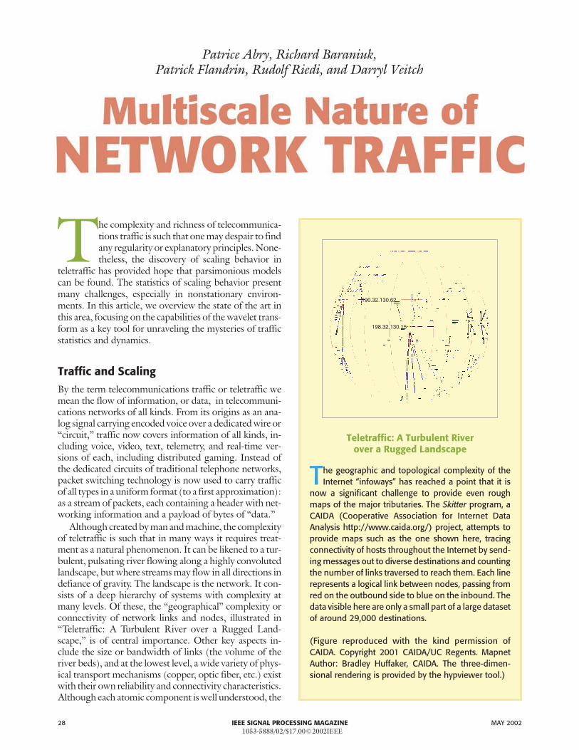
For instance, long memory is a scale invariance phe-nomenon that can be seen in the time series Y t( )describ-ing the data transfer rate over a link at time t. Otherexamples of time series with long memory are the numberof active TCP connections in successive time intervals orthe successive interarrival times of IP packets shown inFig. 1.

The philosophy of scale invariance or “scaling” can beexpressed as the lack of any special characteristic time orspace scale describing fluctuations in Y t( ). Instead one

MAY 2002 IEEE SIGNAL PROCESSING MAGAZINE 29

3

2.5

2

1.5

1

0.5

200 400 600 800 1000 1200 1400 1600

× 104

� 1. A series of interarrival times of TCP connections, showinghighly detailed local structure as well as long memory.

Although created by man andmachine, the complexity ofteletraffic is such that in manyways it requires treatment as anatural phenomenon.

needs to describe the steady progression across scales. Inthe case of traffic such a progression has been found empir-ically and has lead to long memory models and more gen-erally to models with fractal features, as we will explore.

The scale invariant features of traffic can be thought ofas giving precise meaning to the important but potentiallyvague notion of traffic burstiness, which means, roughly, alack of smoothness. In very general terms, burstiness is im-portant because from the field of performance analysis ofnetworks, and in particular that of switches via queueingtheory, we know that increased burstiness results in lowerlevels of resource utilization for a fixed quality of service,and therefore to higher costs. At the engineering level, ser-vice quality refers to metrics such as available bandwidth,data transfer delay, and packet loss. The impact of scaleinvariance extends to network management issues such ascall admission control, congestion control, as well as poli-cies for fairness and pricing.

It is important to distinguish between two canonicalmeanings of the term burstiness, which have their coun-terparts in models and analysis. Again let us take “traffic”to be the data rate Y t( ), nominally in bytes per second,over a link at time t. One kind of burstiness arises fromdependencies over long time periods, which can be madeprecise in terms of the correlation function of Y t( ) (as-suming stationarity and that second order statistics exist).As shown in “Temporal Burstiness in Traffic,” such tem-poral burstiness was explored when scaling was firstfound in packet traffic. More precisely, the well-knownlong-range dependent (LRD) property of traffic is a phe-nomenon defined in terms of temporal correlation,whose network origins are now thought to be quite wellunderstood in terms of the paradigm of heavy tails of filesizes of requested objects, which causes sources to trans-mit over extended periods [36].

A second kind of burstiness describes variability, thesize of fluctuations in value or amplitude, andtherefore concerns small scales. It refers to themarginal distribution of Y t( ), as character-ized, for example, by the ratio of standard de-viation to mean if this exists, as the localsingular behavior of multifractal models (de-scribed in the next section), or alternatively asa heavy tail parameter of the distribution ofthe instantaneous traffic load in the case of in-finite variance models. “Amplitude Burstinessin Traffic” illustrates this latter case for thetime series of successive TCP connection du-rations, derived from measurements takenover a 2 Mb/s access link, made available at theUniversity of Waikato [22]. Even when an ap-parently stationary subset is selected, the vari-ation in value or amplitude is very significantand highly non- Gaussian. Marginals of othertime series do not always yield such extremepower-law tails; however Weibullian orlog-normal behavior is more common thanGaussian, unless the data has already beenhighly aggregated or if scales above a few sec-onds are examined.

The two types of burstiness just describedare quite different. However, often it is con-venient to work not with a stationary serieslike Y t( ), but with its integrated or “countingprocess” equivalent N t( ), which counts theamount of traffic arriving in [ , ]0 t . It is thenimportant to bear in mind that the statisticsof N t( ) are a function both of the temporaland the amplitude burstiness of the rate pro-cess Y t( ).

The next step in this introduction to scalingin traffic is to draw attention to the fact that, al-though at large scales (seconds and beyond) as-tonishingly clear, simple, and relativelywell-understood scaling laws are found, the

30 IEEE SIGNAL PROCESSING MAGAZINE MAY 2002

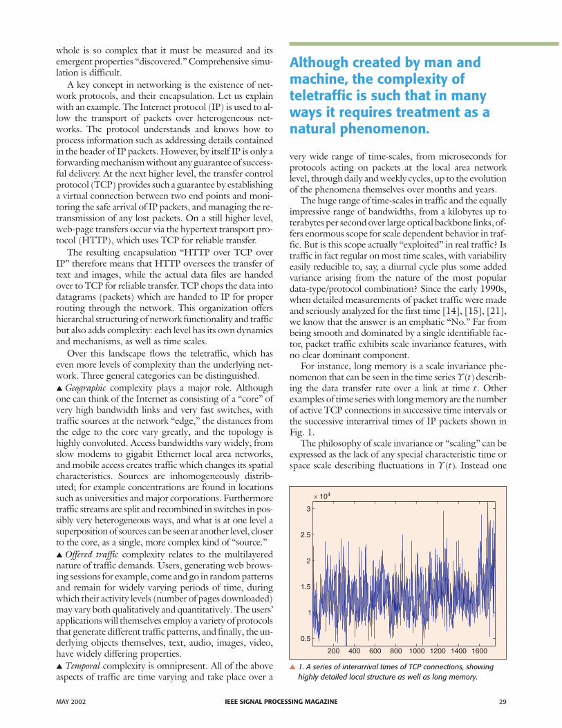
Temporal Burstiness in Traffic

Here, we present an analysis of a standard trace of Ethernet traf-fic, “pAug” from [14]. An entryY k( ) of this time series represents

the number of bytes observed on the Ethernet at Bellcore during thekth time slot of duration δ =12 ms of the measurement. Denote byY m( ) the aggregated series of level m; for exampleY Y Y Y( )( ) ( ( ) ( ) ( )) /3 1 1 2 3 3= + + represents then the average traffic ob-served in time slots of duration 3δ. Through this averaging operator,scale invariance can be illustrated in a simple but powerful way. Fromtop to bottom, the first 512 points of four series are plotted:Y k Y k( ) ( )( )= 1 , Y k( )( )8 , Y k( )( )64 , and Y k( )( )512 , with δ varying fromδ =12 ms to δ =12 8 8 8* * * ms, or 6.1 s.

The decrease in variability with increased smoothing is very slow,consistent with

Var[ ] ( ), 0.4 (0,1)( )Y O mm = ≈ ∈− β β

the so-called “slowly decaying variance” of long memory processes.A wavelet analysis of this series appears in Fig. 7, middle plot.

10,000

5000

050

50

50

50

100

100

100

100

150

150

150

150

200

200

200

200

250

250

250

250

300

300

300

300

350

350

350

350

400

400

400

400

450

450

450

450

500

500

500

500

δ=12 ms

δ=12 * 8 ms

δ=12 * 8 * 8 ms

δ=12 * 8 * 8 * 8 ms

8000600040002000

0

600040002000

0

4000

2000

0

same cannot be said at small scales. This is true, for exam-ple, of the interarrival time series shown in Fig. 1, a discreteseries giving the successive intervals (in milliseconds) be-tween the arrival of new TCP connections. When exam-ined with the naked eye this series may be accused ofhaving long memory, with a marginal slightly deviatingfrom Gaussianity. In reality, in addition to long memory, itcontains much nontrivial scaling structure at small scales(see Fig. 7) which is suggestive of a rich underlying dy-namics of TCP connection creation. Investigation of suchdynamics is beyond the scope of this review, howeverknowledge of its scaling properties lays a foundation for aninformed investigation.

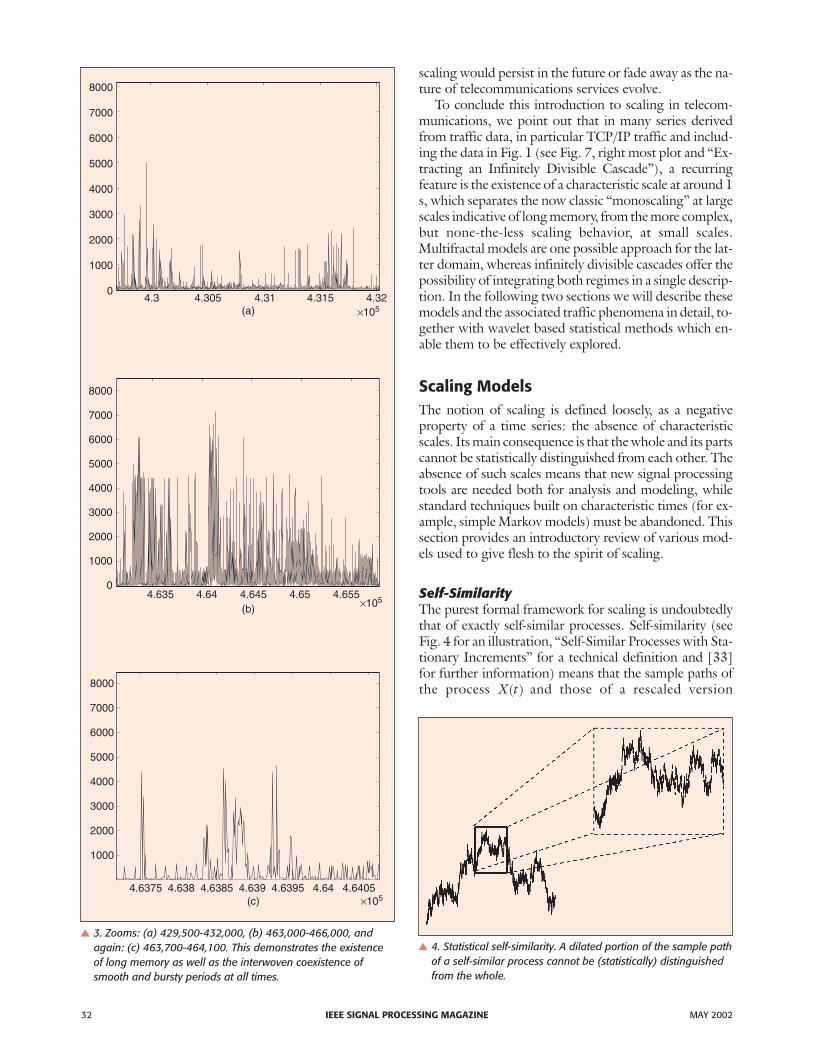
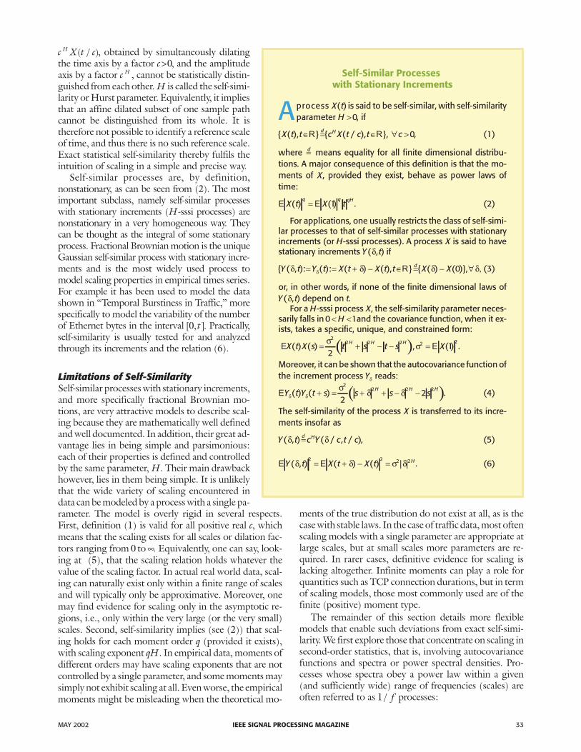
The fact is that much work remains to be done toachieve a clear understanding of traffic scaling over smallscales, which is characterized by far higher variability,more complex and less definitive scaling laws, and the ne-cessity of dealing with non-Gaussian data and hence sta-tistics beyond second order. The high variability on smallscales is shown in Figs. 2 and 3 for a publicly availabletrace collected at the Lawrence Berkeley Laboratory. Thetime series of the number of TCP packets arriving pertime interval has very irregular local structure, as seen inthe blowups in the lower plots. While large-scale behav-ior such as long memory matters for many network de-sign and management issues, understanding small-scalebehavior is particularly important for flow control, per-formance, and efficiency. In terms of network perfor-mance, variability is (almost) always an undesirable

feature of traffic data. Therefore, a key motivation for in-vestigating such scaling is to help identify generatingmechanisms leading to an understanding of their rootcauses in networking terms. If, for example, it wereknown that a certain feature of the TCP protocol was re-sponsible for generating the observed complex scalingbehavior at small scales, then we would be in a position toperhaps eliminate or moderate it via modifications to theprotocol. Alternatively, if a property of certain trafficsource types was the culprit, then we could predict if the

MAY 2002 IEEE SIGNAL PROCESSING MAGAZINE 31

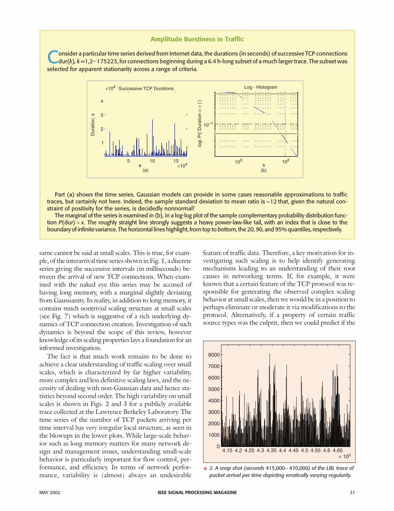
Amplitude Burstiness in Traffic

Consider a particular time series derived from Internet data, the durations (in seconds) of successive TCP connectionsdur(k), k =1,2...175223, for connections beginning during a 6.4 h-long subset of a much larger trace. The subset was

selected for apparent stationarity across a range of criteria.

Part (a) shows the time series. Gaussian models can provide in some cases reasonable approximations to traffictraces, but certainly not here. Indeed, the sample standard deviation to mean ratio is ≈12 that, given the natural con-straint of positivity for the series, is decidedly nonnormal!

The marginal of the series is examined in (b), in a log-log plot of the sample complementary probability distribution func-tion P x( )dur > . The roughly straight line strongly suggests a heavy power-law-like tail, with an index that is close to theboundary of infinite variance. The horizontal lines highlight, from top to bottom, the 20, 90, and 95% quantiles, respectively.

4

3

2

1

Dur

atio

n, s

×104

×104

Successive TCP Durations

5 10 15#

(a)

10–1

100 102s

(b)

log(

Pr[

Dur

atio

n >

] )×

Log - Histogram

8000

7000

6000

5000

4000

3000

2000

1000

04.15 4.2 4.25 4.3 4.35 4.4 4.45 4.5 4.55 4.6 4.65

× 105

� 2. A snap shot (seconds 415 000 470 000, ,− ) of the LBL trace ofpacket arrival per time depicting erratically varying regularity.

scaling would persist in the future or fade away as the na-ture of telecommunications services evolve.

To conclude this introduction to scaling in telecom-munications, we point out that in many series derivedfrom traffic data, in particular TCP/IP traffic and includ-ing the data in Fig. 1 (see Fig. 7, right most plot and “Ex-tracting an Infinitely Divisible Cascade”), a recurringfeature is the existence of a characteristic scale at around 1s, which separates the now classic “monoscaling” at largescales indicative of long memory, from the more complex,but none-the-less scaling behavior, at small scales.Multifractal models are one possible approach for the lat-ter domain, whereas infinitely divisible cascades offer thepossibility of integrating both regimes in a single descrip-tion. In the following two sections we will describe thesemodels and the associated traffic phenomena in detail, to-gether with wavelet based statistical methods which en-able them to be effectively explored.

Scaling ModelsThe notion of scaling is defined loosely, as a negativeproperty of a time series: the absence of characteristicscales. Its main consequence is that the whole and its partscannot be statistically distinguished from each other. Theabsence of such scales means that new signal processingtools are needed both for analysis and modeling, whilestandard techniques built on characteristic times (for ex-ample, simple Markov models) must be abandoned. Thissection provides an introductory review of various mod-els used to give flesh to the spirit of scaling.

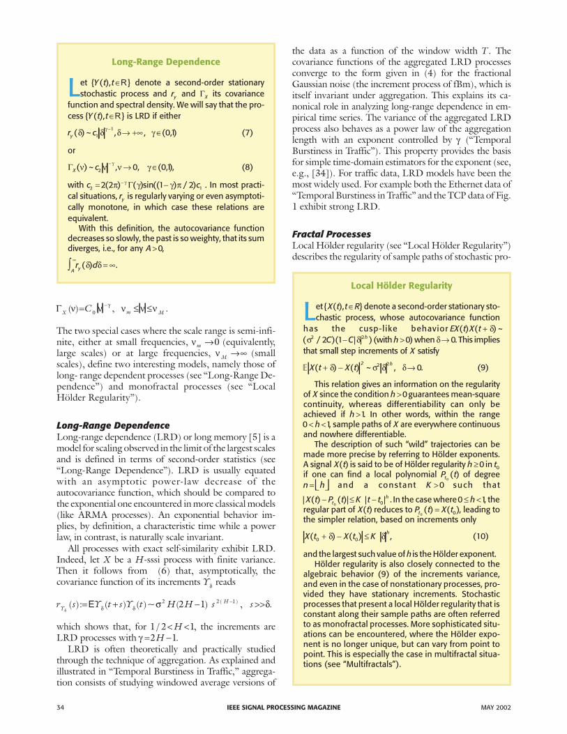
The purest formal framework for scaling is undoubtedlythat of exactly self-similar processes. Self-similarity (seeFig. 4 for an illustration, “Self-Similar Processes with Sta-tionary Increments” for a technical definition and [33]for further information) means that the sample paths ofthe process X t( ) and those of a rescaled version

32 IEEE SIGNAL PROCESSING MAGAZINE MAY 2002

8000

8000

8000

7000

7000

7000

6000

6000

6000

5000

5000

5000

4000

4000

4000

3000

3000

3000

2000

2000

2000

1000

1000

1000

0

0

4.3 4.305 4.31 4.315 4.32(a)

(b)

×105

×105

×105

4.635 4.64 4.645 4.65 4.655

4.6375 4.638 4.6385 4.639 4.6395 4.64 4.6405(c)

� 3. Zooms: (a) 429,500-432,000, (b) 463,000-466,000, andagain: (c) 463,700-464,100. This demonstrates the existenceof long memory as well as the interwoven coexistence ofsmooth and bursty periods at all times.

� 4. Statistical self-similarity. A dilated portion of the sample pathof a self-similar process cannot be (statistically) distinguishedfrom the whole.

c X t cH ( / ), obtained by simultaneously dilatingthe time axis by a factor c>0, and the amplitudeaxis by a factor c H , cannot be statistically distin-guished from each other. H is called the self-simi-larity or Hurst parameter. Equivalently, it impliesthat an affine dilated subset of one sample pathcannot be distinguished from its whole. It istherefore not possible to identify a reference scaleof time, and thus there is no such reference scale.Exact statistical self-similarity thereby fulfils theintuition of scaling in a simple and precise way.

Self-similar processes are, by definition,nonstationary, as can be seen from (2). The mostimportant subclass, namely self-similar processeswith stationary increments (H-sssi processes) arenonstationary in a very homogeneous way. Theycan be thought as the integral of some stationaryprocess. Fractional Brownian motion is the uniqueGaussian self-similar process with stationary incre-ments and is the most widely used process tomodel scaling properties in empirical times series.For example it has been used to model the datashown in “Temporal Burstiness in Traffic,” morespecifically to model the variability of the numberof Ethernet bytes in the interval [ , ]0 t . Practically,self-similarity is usually tested for and analyzedthrough its increments and the relation (6).

Self-similar processes with stationary increments,and more specifically fractional Brownian mo-tions, are very attractive models to describe scal-ing because they are mathematically well definedand well documented. In addition, their great ad-vantage lies in being simple and parsimonious:each of their properties is defined and controlledby the same parameter, H. Their main drawbackhowever, lies in them being simple. It is unlikelythat the wide variety of scaling encountered indata can be modeled by a process with a single pa-rameter. The model is overly rigid in several respects.First, definition (1) is valid for all positive real c, whichmeans that the scaling exists for all scales or dilation fac-tors ranging from 0 to ∞. Equivalently, one can say, look-ing at (5), that the scaling relation holds whatever thevalue of the scaling factor. In actual real world data, scal-ing can naturally exist only within a finite range of scalesand will typically only be approximative. Moreover, onemay find evidence for scaling only in the asymptotic re-gions, i.e., only within the very large (or the very small)scales. Second, self-similarity implies (see (2)) that scal-ing holds for each moment order q (provided it exists),with scaling exponent qH. In empirical data, moments ofdifferent orders may have scaling exponents that are notcontrolled by a single parameter, and some moments maysimply not exhibit scaling at all. Even worse, the empiricalmoments might be misleading when the theoretical mo-

ments of the true distribution do not exist at all, as is thecase with stable laws. In the case of traffic data, most oftenscaling models with a single parameter are appropriate atlarge scales, but at small scales more parameters are re-quired. In rarer cases, definitive evidence for scaling islacking altogether. Infinite moments can play a role forquantities such as TCP connection durations, but in termof scaling models, those most commonly used are of thefinite (positive) moment type.

The remainder of this section details more flexiblemodels that enable such deviations from exact self-simi-larity. We first explore those that concentrate on scaling insecond-order statistics, that is, involving autocovariancefunctions and spectra or power spectral densities. Pro-cesses whose spectra obey a power law within a given(and sufficiently wide) range of frequencies (scales) areoften referred to as 1 / f processes:

MAY 2002 IEEE SIGNAL PROCESSING MAGAZINE 33

Self-Similar Processeswith Stationary Increments

Aprocess X t( ) is said to be self-similar, with self-similarityparameter H >0, if

{ ( ), } { ( / ), },X t t c X t c t cd H∈ = ∈ ∀ >R R 0, (1)

where =d means equality for all finite dimensional distribu-tions. A major consequence of this definition is that the mo-ments of X, provided they exist, behave as power laws oftime:

E EX t X tq q qH( ) ( )= 1 . (2)

For applications, one usually restricts the class of self-simi-lar processes to that of self-similar processes with stationaryincrements (or H-sssi processes). A process X is said to havestationary increments Y t( , )δ if

{ ( , ): ( ): ( ) ( ), } { ( ) ( )},Y t Y t X t X t t X Xdδ δ δ δ,δ= = + − ∈ = − ∀R 0 (3)

or, in other words, if none of the finite dimensional laws ofY t( , )δ depend on t.

For a H-sssi process X, the self-similarity parameter neces-sarily falls in 0 1< <H and the covariance function, when it ex-ists, takes a specific, unique, and constrained form:

( )E EX t X s t s t s XH H H( ) ( ) , ( )= + − − =σ σ2

2 2 2 2 2

21 .

Moreover, it can be shown that the autocovariance function ofthe increment process Yδ reads:

( )EY t Y t s s s sH H Hδ δ

σ δ δ( ) ( )+ = + + − −2

2 2 2

22 . (4)

The self-similarity of the process X is transferred to its incre-ments insofar as

Y t c Y c t cd H( , ) ( / , / )δ δ= , (5)

E EY t X t X t H( , ) ( ) ( ) | |δ δ σ δ2 2 2 2= + − = . (6)

ΓX m MC( ) ,ν ν ν ν νγ= ≤ ≤−0 .

The two special cases where the scale range is semi-infi-nite, either at small frequencies, νm →0 (equivalently,large scales) or at large frequencies, ν M →∞ (smallscales), define two interesting models, namely those oflong- range dependent processes (see “Long-Range De-pendence”) and monofractal processes (see “LocalHölder Regularity”).

Long-range dependence (LRD) or long memory [5] is amodel for scaling observed in the limit of the largest scalesand is defined in terms of second-order statistics (see“Long-Range Dependence”). LRD is usually equatedwith an asymptotic power-law decrease of theautocovariance function, which should be compared tothe exponential one encountered in more classical models(like ARMA processes). An exponential behavior im-plies, by definition, a characteristic time while a powerlaw, in contrast, is naturally scale invariant.

All processes with exact self-similarity exhibit LRD.Indeed, let X be a H-sssi process with finite variance.Then it follows from (6) that, asymptotically, thecovariance function of its increments Yδ reads

r s Y t s Y t H H s sYH

δ δ δ σ δ( ): ( ) ( )~ ( ) ,( )= + − >>−E 2 2 12 1 .

which shows that, for 1 2 1/ < <H , the increments areLRD processes with γ = −2 1H .

LRD is often theoretically and practically studiedthrough the technique of aggregation. As explained andillustrated in “Temporal Burstiness in Traffic,” aggrega-tion consists of studying windowed average versions of

the data as a function of the window width T . Thecovariance functions of the aggregated LRD processesconverge to the form given in (4) for the fractionalGaussian noise (the increment process of fBm), which isitself invariant under aggregation. This explains its ca-nonical role in analyzing long-range dependence in em-pirical time series. The variance of the aggregated LRDprocess also behaves as a power law of the aggregationlength with an exponent controlled by γ (“TemporalBurstiness in Traffic”). This property provides the basisfor simple time-domain estimators for the exponent (see,e.g., [34]). For traffic data, LRD models have been themost widely used. For example both the Ethernet data of“Temporal Burstiness in Traffic” and the TCP data of Fig.1 exhibit strong LRD.

Local Hölder regularity (see “Local Hölder Regularity”)describes the regularity of sample paths of stochastic pro-

34 IEEE SIGNAL PROCESSING MAGAZINE MAY 2002

Long-Range Dependence

Let { ( ), }Y t t∈R denote a second-order stationarystochastic process and ry and ΓX its covariance

function and spectral density. We will say that the pro-cess { ( ), }Y t t∈R is LRD if either

r cy ( )~ , , ( , )δ δ δ γγ1

1 01− → +∞ ∈ (7)

or

ΓX c( )~ , , ( , )ν ν ν γγ2 0 01− → ∈ , (8)

with c c2 12 2 1 2= −−( ) ( ) (( ) / )π γ γ πγ Γ sin . In most practi-cal situations, ry is regularly varying or even asymptoti-cally monotone, in which case these relations areequivalent.

With this definition, the autocovariance functiondecreases so slowly, the past is so weighty, that its sumdiverges, i.e., for any A >0,

r dyA

∞∫ = ∞( )δ δ .

Local Hölder Regularity

Let{ ( ), }X t t R∈ denote a second-order stationary sto-chastic process, whose autocovariance function

has the cusp-like behavior EX t X t( ) ( )~+ δ( / )( | | )σ δ2 22 1C C h− (with h >0) when δ→ 0. This impliesthat small step increments of X satisfy

� X t X t h( ) ( ) ~ ,+ − →δ σ δ δ2 2 2 0. (9)

This relation gives an information on the regularityof X since the condition h >0guarantees mean-squarecontinuity, whereas differentiability can only beachieved if h >1. In other words, within the range0 1< <h , sample paths of X are everywhere continuousand nowhere differentiable.

The description of such “wild” trajectories can bemade more precise by referring to Hölder exponents.A signal X t( ) is said to be of Hölder regularity h ≥0 in t0if one can find a local polynomial P tt0

( ) of degree n h= and a constant K >0 such that

| ( ) ( )| | | .X t P t K t tth− ≤ −

0 0 In the case where0 1≤ <h , theregular part of X t( ) reduces to P t X tt0 0( ) ( )= , leading tothe simpler relation, based on increments only

X t X t K h( ) ( )0 0+ − ≤δ δ , (10)

and the largest such value of h is the Hölder exponent.Hölder regularity is also closely connected to the

algebraic behavior (9) of the increments variance,and even in the case of nonstationary processes, pro-vided they have stationary increments. Stochasticprocesses that present a local Hölder regularity that isconstant along their sample paths are often referredto as monofractal processes. More sophisticated situ-ations can be encountered, where the Hölder expo-nent is no longer unique, but can vary from point topoint. This is especially the case in multifractal situa-tions (see “Multifractals”).

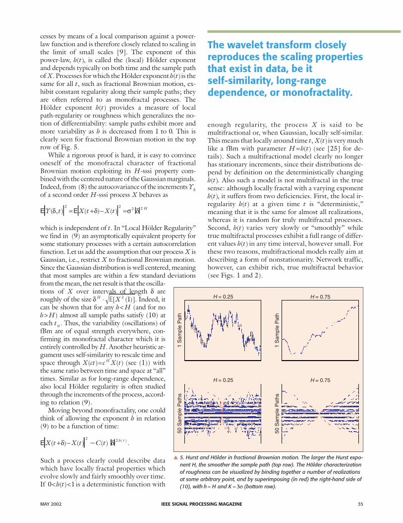
cesses by means of a local comparison against a power-law function and is therefore closely related to scaling inthe limit of small scales [9]. The exponent of thispower-law, h t( ), is called the (local) Hölder exponentand depends typically on both time and the sample pathof X. Processes for which the Hölder exponent h t( )is thesame for all t, such as fractional Brownian motion, ex-hibit constant regularity along their sample paths; theyare often referred to as monofractal processes. TheHölder exponent h t( ) provides a measure of localpath-regularity or roughness which generalizes the no-tion of differentiability: sample paths exhibit more andmore variability as h is decreased from 1 to 0. This isclearly seen for fractional Brownian motion in the toprow of Fig. 5.

While a rigorous proof is hard, it is easy to convinceoneself of the monofractal character of fractionalBrownian motion exploiting its H-sssi property com-bined with the centered nature of the Gaussian marginals.Indeed, from (8) the autocovariance of the increments Yδof a second order H-sssi process X behaves as

E EY t X t X t H( , ) ( ) ( )δ δ σ δ2 2 2 2= + − =

which is independent of t. In “Local Hölder Regularity”we find in (9) an asymptotically equivalent property forsome stationary processes with a certain autocorrelationfunction. Let us add the assumption that our process X isGaussian, i.e., restrict X to fractional Brownian motion.Since the Gaussian distribution is well centered, meaningthat most samples are within a few standard deviationsfrom the mean, the net result is that the oscilla-tions of X over intervals of length δ areroughly of the size δ H X⋅ �[ ( )]2 1 . Indeed, itcan be shown that for any h H< (and for noh H> ) almost all sample paths satisfy (10) ateach t 0 . Thus, the variability (oscillations) offBm are of equal strength everywhere, con-firming its monofractal character which it isentirely controlled by H. Another heuristic ar-gument uses self-similarity to rescale time andspace through X ct c X tH( ) ( )= (see (1)) withthe same ratio between time and space at “all”times. Similar as for long-range dependence,also local Hölder regularity is often studiedthrough the increments of the process, accord-ing to relation (9).

Moving beyond monofractality, one couldthink of allowing the exponent h in relation(9) to be a function of time:

E X t X t C t h t( ) ( ) ~ ( ) ( )+ −δ δ2 2 .

Such a process clearly could describe datawhich have locally fractal properties whichevolve slowly and fairly smoothly over time.If 0 1< <h t( ) is a deterministic function with

enough regularity, the process X is said to bemultifractional or, when Gaussian, locally self-similar.This means that locally around time t, X t( )is very muchlike a fBm with parameter H h t= ( ) (see [25] for de-tails). Such a multifractional model clearly no longerhas stationary increments, since their distributions de-pend by definition on the deterministically changingh t( ). Also such a model is not multifractal in the truesense: although locally fractal with a varying exponenth t( ), it suffers from two deficiencies. First, the local ir-regularity h t( ) at a given time t is “deterministic,”meaning that it is the same for almost all realizations,whereas it is random for truly multifractal processes.Second, h t( ) varies very slowly or “smoothly” whiletrue multifractal processes exhibit a full range of differ-ent values h t( ) in any time interval, however small. Forthese two reasons, multifractional models really aim atdescribing a form of nonstationarity. Network traffic,however, can exhibit rich, true multifractal behavior(see Figs. 1 and 2).

MAY 2002 IEEE SIGNAL PROCESSING MAGAZINE 35

1 S

ampl

e P

ath

1 S

ampl

e P

ath

50 S

ampl

e P

aths

50 S

ampl

e P

aths

H = 0.25 H = 0.75

H = 0.25 H = 0.75

� 5. Hurst and Hölder in fractional Brownian motion. The larger the Hurst expo-nent H, the smoother the sample path (top row). The Hölder characterizationof roughness can be visualized by binding together a number of realizationsat some arbitrary point, and by superimposing (in red) the right-hand side of(10), with h H= and K = 3σ (bottom row).

The wavelet transform closelyreproduces the scaling propertiesthat exist in data, be itself-similarity, long-rangedependence, or monofractality.

When the regularity h t( ) is itself a highly irregular functionof t, possibly even a random process rather than a constantor a fixed deterministic function, the process X is said to bemultifractal. In such situations, the fluctuations in regularityalong paths are no longer described in terms of a functionh t( ) but through the so-called multifractal spectrum D h( )(see “Multifractals” and [9] and [29]). Teletraffic time se-ries, for example those in Figs. 1 and 2, in fact often have lo-cal Hölder exponents h t( ) which change erratically withlocation t. Such behavior is loosely termed multifractal. Amodel class which is rich enough to capture multifractalproperties is that of multiplicative cascades. One of the mostcelebrated examples is that of the binomial cascade X, de-fined here for convenience on [ , ]0 1 through:

X k X k M X k

X k

n n dk

n n(( ) / ) ( / ) ( (( ) / )

( /

2 1 2 2 2 1 21 12

1+ − = +

−

+ + +

2

1 01

1

n

dki

i

n

M X Xi

))

( ( ) ( )).= ⋅ −=

+

∏(11)

Here the Mki

iare independent positive random vari-

ables called the multipliers such that “siblings” add up toone: M Mk

nk

n2

12 1

1 1++

++ = . Thus, (11) “repartitions” the in-crements of X iteratively. Setting X( )0 0= and X( )1 1= (forconvenience) defines the process on [ , ]0 1 . This is a partic-ular incarnation of a general approach to the generationof multifractal processes, namely the iteration of a multi-plicative procedure. Note that all increments are positiveand that the aspect ratios, given by the Mki i,

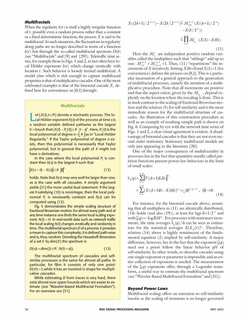
, depend ex-plicitly on the location where the rescaling is done. This isin stark contrast to the scaling of fractional Brownian mo-tion and the relation (5) for self-similarity and is the mostimmediate reason for the multifractal structure of cas-cades. An illustration of this construction procedure aswell as an example of resulting sample path is shown onFig. 6. Comparing by eye with the network time series ofFigs. 1 and 2, a clear visual agreement is evident. A disad-vantage of binomial cascades is that they are not even sec-ond order stationary. Stationary multifractal models areonly just appearing in the literature [20].

One of the major consequences of multifractality inprocesses lies in the fact that quantities usually called par-tition functions present power-law behaviors in the limitof small scales:

S q Y k

X k X k

q

k

k

δ

δ

δ

δ δ

δ δ

( ) (( ) , ))

| (( ) ) ( )

/

/

= +

= + −

=

=

∑

∑

1

1

1

1

1

1

| | | , | | .~ ( )qq

qc− →−δ δζ 1 0(14)

For instance, for the binomial cascade above, assum-ing that all multipliers in (11) are identically distributed,(14) holds (and also (19)), at least for lags δ= /1 2 n andwithζ( ) logq M q=− E . For processes with stationary incre-ments, the time averages S qδ δ( ) / can be seen as estima-tors for the statistical averages E X t q| ( )|δ . Therefore,relation (14) above is highly reminiscent of the funda-mental equation (2) implied by self-similarity. A majordifference, however, lies in the fact that the exponent ζ( )qneed not a priori follow the linear behavior qH ofself-similarity. In other words, to describe cascades usingone single exponent or parameter is impossible and an en-tire collection of exponents is needed. The measurementof the ζ( )q exponents offer, through a Legendre trans-form, a useful way to estimate the multifractal spectrum(see “Wavelet-Based Multifractal Formalism” and [31]).

Multifractal scaling offers an extension to self-similarityinsofar as the scaling of moments is no longer governed

36 IEEE SIGNAL PROCESSING MAGAZINE MAY 2002

Multifractals

Let { ( ), }X t t∈R denote a stochastic process. The lo-cal Hölder exponent h s( )of the process at time s is

a random variable defined pathwise as the largesth >0such that | ( ) ( )| | | .X t P t K t ss

h− ≤ − Here, P ts( ) is thelocal polynomial of degree n h= as in “Local HolderRegularity.” If the Taylor polynomial of degree n ex-ists, then this polynomial is necessarily that Taylorpolynomial; but in general the path of X might nothave n derivatives.

In the case where the local polynomial Ps is con-stant then h s( ) is the largest h such that

X s X s K h( ) ( )+ − ≤δ δ (12)

holds. Note that h s( ) may very well be larger than one,as is the case with all cascades. A simple argumentyields [31] the more useful dual statement: if the larg-est h satisfying (10) is noninteger, then the local poly-nomial Ps is necessarily constant and h s( ) can becomputed using (12).

Fig. 5 demonstrates the simple scaling structure offractional Brownian motion; for almost every path and atany time instance one finds the same local scaling expo-nent: h t H( ) = . In real-world data such as network trafficthe local scaling h t( ) changes erratically and randomly intime. The multifractal spectrum Dof a process X providesa mean to capture this complexity; it is defined path-wiseand is, thus, random. Denoting the Hausdorff dimensionof a set E by dim( )E the spectrum is

D a t h t a( ): dim({ : ( ) })= ∈ =R . (13)

The multifractal spectrum of cascades and self-similar processes is the same for almost all paths. Inparticular, for fBm it consists of only one point:D H( ) =1, while it has an inverted-U shape for multipli-cative cascades.

While estimating D from traces is very hard, thereexist almost sure upper bounds which are easier to es-timate (see “Wavelet-Based Multifractal Formalism”).For an overview see [31].

MAY 2002 IEEE SIGNAL PROCESSING MAGAZINE 37

(a)

Dj,k0

Dj+ k1,2 0Dj+ k1,2 +10

Dj k+2,4 0Dj k+2,4 +10

Dj k+2,4 +20Dj k+2,4 +30

k ′0=0

k ′1=0 k ′1=1 k ′1=0 k ′1=1

k ′0=1

M 00

M 10 • M 0

0

M 20 •M 1

0 •M 00

M 20 •M 1

0 •M 00

M 20 •M 1

0 •M 00 M 2

3 •M 11 •M 0

0

M 11 • M 0

0

0 1

0 0.5 1

0 0.25 0.5 0.75 1

50

40

30

20

10

00 0.2 0.4 0.6 0.8 1

(b)

(c)

� 6. Binomial cascade. (a) Dyadic tree-based construction, (b) first three intermediate stages (values of the measure on coarsest inter-vals), and (c) a sample path.

Infinitely Divisible Cascades

Self-similarity implies that the probability density func-tion (pdf) pδ of the increments Xδ at scale δ, is a dilated

version of the pdf of those at a larger scale δ':p x p xδ δα α( ) ( / ) ( / )'= 1 0 0 where the dilation factor isunique: α δ δ0 =( / ')H . In the cascade model, the key ingre-dient is that there is no longer a unique factor but a collec-tion of dilation factors α ; consequently p

δwill result from a

weighted sum of dilated incarnations of pδ:

p x G ln px

dδ δ δ δα

α αα( ) ( ) ln,=

∫ ′

1.

The function Gδ δ, ′ is called the kernel or the propagatorof the cascade. A change of variable shows that the defini-tion above relates the pdfs p

δand pδ ′ of the log-incre-

ments ln| |Xδ at different scales through a convolution withthe propagator:

p x G p x dG p

δ δ δ δ

δ δ δ

α α α( ) ( ) ( ln ) ln( * )(

,

,

ln ln lnln

= −=

′ ′

′ ′

∫α).

(15)

Infinite divisibility implies by definition that no scale be-tween δ and δ′ plays any specific role, i.e., if scale δ′′ lies be-tween scales δand δ′ thenG G Gδ δ δ δ δ δ, , ,*′ ′′ ′′ ′= . This convolutiveproperty implies that propagators can be written in terms ofan elementary functionG0 convolved with itself a number oftimes, where that number depends on δ and δ′

G G n nδ δ

δ δα α,*( ( ) ( ))( ) [ ( )]′

− ′=ln ln0 .

Here, G n* denotes n fold convolution of G with itself.Using the Laplace transform

~( ),G qδ δ′ of Gδ δ, ′, this can be

rewrit ten as~

( ) exp{ ( )( ( ) ( ))},G q H q n nδ δ δ δ′ = − ′ , withH q G q( ) ln

~( )= . This yields (compare with eq. (20)): the fol-

lowing relations, fundamental for the analysis [39]:

ln ( ) ( )� X H q n Kqqδ δ= + (16)

ln( )( )

ln ,� XH qH p

Xq pq pδ δ κ= +E . (17)

A possible interpretation of this relation is that thefunction G0 defines the elementary step of the cascadewhereas the quantity n n( ) ( )δ δ− ′ quantifies the numberof times this elementary step is to be applied to proceedfrom scales δ to δ′. The derivative of nwith respect to δde-scribes in some sense the speed of the cascade at scale δ.When the function n takes the specific form n( ) lnδ δ= , theinfinitely divisible cascade is said to be scale invariant andreduces to multifractal scaling. The exponents ζ( )q asso-ciated to the multifractal spectrum are then related to theLaplace transform of the propagator through ξ( ) ( )q H q=(see “Infinitely Divisble Cascades”). As detailed in thetext, self-similarity is also included as an even more spe-cial case. For further details on infinitely divisible cascade,see [39].

by one single exponent H but by a collection of expo-nents. However, it maintains a key feature: moments be-have as power laws of the scales. When analyzing actualdata, it may very well be observed that this is not the case,see, e.g., [39]. To account for those situations, the infi-nitely divisible cascade (IDC) model provides an extra de-gree of freedom.

The concept of IDCs was first introduced by Castaing in[6] and rephrased in the wavelet framework in [4]. “Infi-nitely Divisible Cascades” briefly recalls its definition, con-sequences, and relations to other models. The central anddefining quantity of an IDC is the propagator or kernelG δ δ, ′. Infinite divisibility generalizes the concept of self-simi-larity; it simply says that the marginal distributions at differ-ent scales are related to each other through a simpleconvolution with the propagatorG; thus,G completely cap-tures and controls the multiscale statistics. Leaving details to“Infinitely Divisible Cascades,” let us be explicit in the caseof self-similarity where the propagator takes a particularsimple form due to (1): G δ δ, ′ is a Dirac function. In moreprecise terms, the distribution at scale δ′ is obtained byconvolving the distribution at scale δ withG Hδ δ α δ α δ δ, ( ) ( ln( / ))′ = − ′ln ln ). Since the Laplace trans-form reads as ~ ( ) exp{ ( / )},G q qHδ δ δ δ′ = ′ln we may interpret

G δ δ, ′ as the ln( / )δ δ′ -fold self-convolution of an elementarypropagatorG0 which describes a “unit change of scale.” Forcomparison, we note:

Self-similarity

E| ( )| | | ( ln )X t c c qHqq

qHqδ δ δ= = exp (18)

Multifractal scaling

E| ( )| | | ( ( )ln )( )X t c c qqq

qqδ

ζδ ζ δ= = exp (19)

Infinitely divisible cascade

E| ( )| ( ( ) ( ))X t c H q nqqδ δ= exp (20)

where the function n( )δ is not necessarily lnδ, just as thefunction H q( ) is not a priori qH.

Wavelets for Analysis and InferenceWe saw from the previous section that diverse signaturesof scaling can be observed both with respect to time (reg-ularity of sample paths, slow decay of correlation func-tions,...), or to frequency/scale (power-law spectrum,aggregation, zooming, small scale increments, etc). This

38 IEEE SIGNAL PROCESSING MAGAZINE MAY 2002

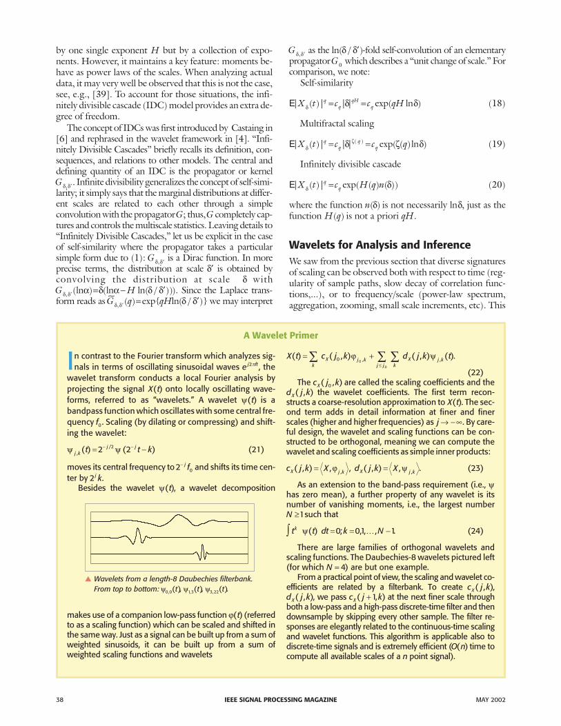
A Wavelet Primer

In contrast to the Fourier transform which analyzes sig-nals in terms of oscillating sinusoidal waves e j ft2π , the

wavelet transform conducts a local Fourier analysis byprojecting the signal X t( ) onto locally oscillating wave-forms, referred to as “wavelets.” A wavelet ψ( )t is abandpass function which oscillates with some central fre-quency f0. Scaling (by dilating or compressing) and shift-ing the wavelet:

ψ ψj kj jt t k,/( ) ( )= −− −2 22 (21)

moves its central frequency to2 0− j f and shifts its time cen-

ter by 2 j k.Besides the wavelet ψ( )t , a wavelet decomposition

makes use of a companion low-pass function ϕ( )t (referredto as a scaling function) which can be scaled and shifted inthe same way. Just as a signal can be built up from a sum ofweighted sinusoids, it can be built up from a sum ofweighted scaling functions and wavelets

X t c j k d j k tk

X j kj j k

X j k( ) ( , ) ( , ) ( ), ,= +∑ ∑ ∑≤

0 0

0

ϕ ψ .

(22)The c j kX( , )0 are called the scaling coefficients and the

d j kX( , ) the wavelet coefficients. The first term recon-structs a coarse-resolution approximation to X t( ). The sec-ond term adds in detail information at finer and finerscales (higher and higher frequencies) as j → −∞. By care-ful design, the wavelet and scaling functions can be con-structed to be orthogonal, meaning we can compute thewavelet and scaling coefficients as simple inner products:

c j k X d j k XX j k X j k( , ) , , ( , ) ,, ,= =ϕ ψ . (23)

As an extension to the band-pass requirement (i.e., ψhas zero mean), a further property of any wavelet is itsnumber of vanishing moments, i.e., the largest numberN ≥1such that

t t dt k Nk∫ = = −ψ( ) ; , , ,0 01 1K . (24)

There are large families of orthogonal wavelets andscaling functions. The Daubechies-8 wavelets pictured left(for which N = 4) are but one example.

From a practical point of view, the scaling and wavelet co-efficients are related by a filterbank. To create c j kX( , ),d j kX( , ), we pass c j kX( , )+1 at the next finer scale throughboth a low-pass and a high-pass discrete-time filter and thendownsample by skipping every other sample. The filter re-sponses are elegantly related to the continuous-time scalingand wavelet functions. This algorithm is applicable also todiscrete-time signals and is extremely efficient (O n( ) time tocompute all available scales of a n point signal).

� Wavelets from a length-8 Daubechies filterbank.From top to bottom: ψ0 0, ( )t , ψ1 3, ( )t , ψ3 22, ( )t .

suggests that to identify and characterize scaling an ap-proach which combines time and frequency/scale, andwhich formalizes properly the idea of a simultaneousanalysis at a continuum of scales, should be taken. Inthis respect, wavelet analysis appears as the most natu-ral framework.

By definition, wavelet analysis (see “A Wavelet Primer”for basics and [18] for a comprehensive survey) acts as amathematical microscope which allows one to zoom inon fine structures of a signal or, alternatively, to reveallarge scale structures by zooming out. Therefore, when asignal or a process obeys some form of scale invariance,some self-reproducing property under dilation, waveletsare naturally able to reveal it by a corresponding self-re-producing property across scales. Moreover, the time-de-pendence of the wavelet transform allows for atime-localization of scaling features.

In its discrete version operating on dyadic scales, thewavelet transform (WT) is a rigorous and invertible wayof performing a multiresolution analysis, a splitting of asignal into a low-pass approximation and a high-pass de-tail, at any level of resolution. Iterating the procedure,one arrives at a representation which consists of alow-resolution approximation and a collection of detailsof higher and higher resolution. From the perspective ofmore classical methods used for scaling data, iteratinglow-pass approximations, at coarser and coarser resolu-tions, is an implicit way of aggregating data, whereasevaluating high-pass details, as differences between ap-proximations, is nothing but a refined way of comput-ing increments (of order N for a wavelet with Nvanishing moments). Combining these two key ele-ments makes of multiresolution a natural language forscaling processes.

As explained earlier, self-similarity is the canonical ref-erence model for scaling behavior. Self-similar processeswith stationary increments are traditionally analyzedthrough their increments, however, reasons for resortingto wavelets are at least threefold:� 1) Scaling: Due to its built-in scaling structure, thewavelet transform reproduces any scaling present in thedata, with a geometrical progression of all (existing) mo-ments across scales, as

E Ed j k d kX

q

X

q jq H( , ) ( , ) ( / )= ⋅ +0 2 1 2 . (25)

� 2) Stationarization: Due to the bandpass nature of ad-missible wavelets, sequences of wavelet coefficients canbe seen as (filtered) increment processes at differentscales: this makes the analysis extensible to nonstationaryprocesses with stationary increments (like H-sssi pro-cesses), resulting in stationary sequences at each scale.� 3) Almost decorrelation: Whereas direct manipulationof LRD processes is hampered by slowly-decaying corre-lations, it turns out that [11], [37]

Ed j k d j k m C j m mX XH N( , ) ( , )~ ( )| | , | |+ →∞−2 2 ,

N being the number of vanishing moments of the wavelet.Under the mild condition N H≥ +1 2/ , global LRD exist-ing among the increments of H-sssi processes can thus beturned, at each scale, into short-range dependence.

Another advantage is that, due to the frequency inter-pretation of wavelets, wavelet analysis can serve as a basisfor useful substitutes for spectral analysis. Indeed, it canbe shown that for stationary processes X with powerspectrum ΓX( )ν , we have

Ed j k dX Xj j( , ) ( ) | ( )|2 22 2=∫Γ Ψν ν ν.

When in addition X is a long range dependent process,this yields

Ed j k C jXj( , ) ~ ,

22′ →+∞α , (28)

MAY 2002 IEEE SIGNAL PROCESSING MAGAZINE 39

Wavelet Analysis of Second-Order Scaling

Scaling processes (be they LRD,1/ f -type, mono- ormultifractal) share the property of exhibiting

power-law spectra in some frequency range, whencethe idea of estimating scaling exponents from a spec-tral estimation. The wavelet transform offers an alter-native to classical spectrum analysis [2], based on apower-law behavior of the wavelet detail variancesacross scales

E d j k CXj( , ) ~

22 γ , (26)

reminiscent of (25) with q =2 for self-similarity, (28) forlong-range dependence, and (30) for monofractality.These are all suggestive of a linear relationshiplog ( , ) ~2

2�d j k j CX γ + in a log-log plot.The stationarization property together with the al-

most decorrelation property (see points 2 and 3 intext) justify that the variance involved in (26) can be ef-ficiently estimated on the basis of the simple empiricalestimate:

µ jj k

n

Xnd j k

j

==

∑1

1

2( , ) , (27)

where nj is the number of coefficients available at oc-tave j. The graph of log2 µ j against j (together withproper confidence intervals) is referred to as the (sec-ond-order) logscale diagram (LD) [3]. Examples aregiven in Fig. 7. Straight lines in such diagrams can beunderstood as evidence for the existence of scaling inanalyzed data, while the range of scales involved givesinformation on its precise nature (self-similarity, longmemory). Estimation of scaling exponents can be car-ried out from such graphs via weighted linear-fit tech-niques (see [3], [38], and [1] for details). The possibilityof varying the number of vanishing moments of themother wavelet bring robustness to the analysis pro-cedure against nonstationarities.

and it can be shown [2] that the corresponding waveletcoefficients are also short-range dependent as soon asN ≥α / 2.

Wavelet coefficients are also useful to study Hölderregularity. This relies on the fact that if X is Hölder con-tinuous of degree h t( )at t then the wavelet coefficients at tdecay as

| ( , )| ( ( ) / )d j kXj h t≤ +2 1 2 (29)

as the intervals [ ,( ) ]k kj j2 1 2+ close in on t ( j →−∞). Un-der certain conditions, the bound is asymptotically tight[13], [7]. For monofractal processes, that is for processes

for which Hölder exponents h t( ) remain constant alongsample paths, we have the following relation:

Ed j k C jXj h( , ) ~ ,( )

22 12′′ + →−∞,

(30)

to be compared to (25) and (28).To summarize, the wavelet transform closely reproduces

the scaling properties that exist in data, be it self-similarity,long-range dependence, or monofractality, and, at the sametime, replaces one single poorly behaved (nonstationary,LRD) time series by a collection of much better behaved se-quences (stationary, SRD), amenable to standard statisticaltools. Therefore, second-order statistical scaling propertiescan be efficiently estimated from marginalized scalograms(squared wavelet coefficients averaged over time), circum-venting the difficulties usually attached to scaling processes.Using this idea, “Wavelet Analysis of Second-OrderScaling” details the steps leading to an estimation of the ex-ponent of second order scaling, in a log-log plot known asthe logscale diagram.

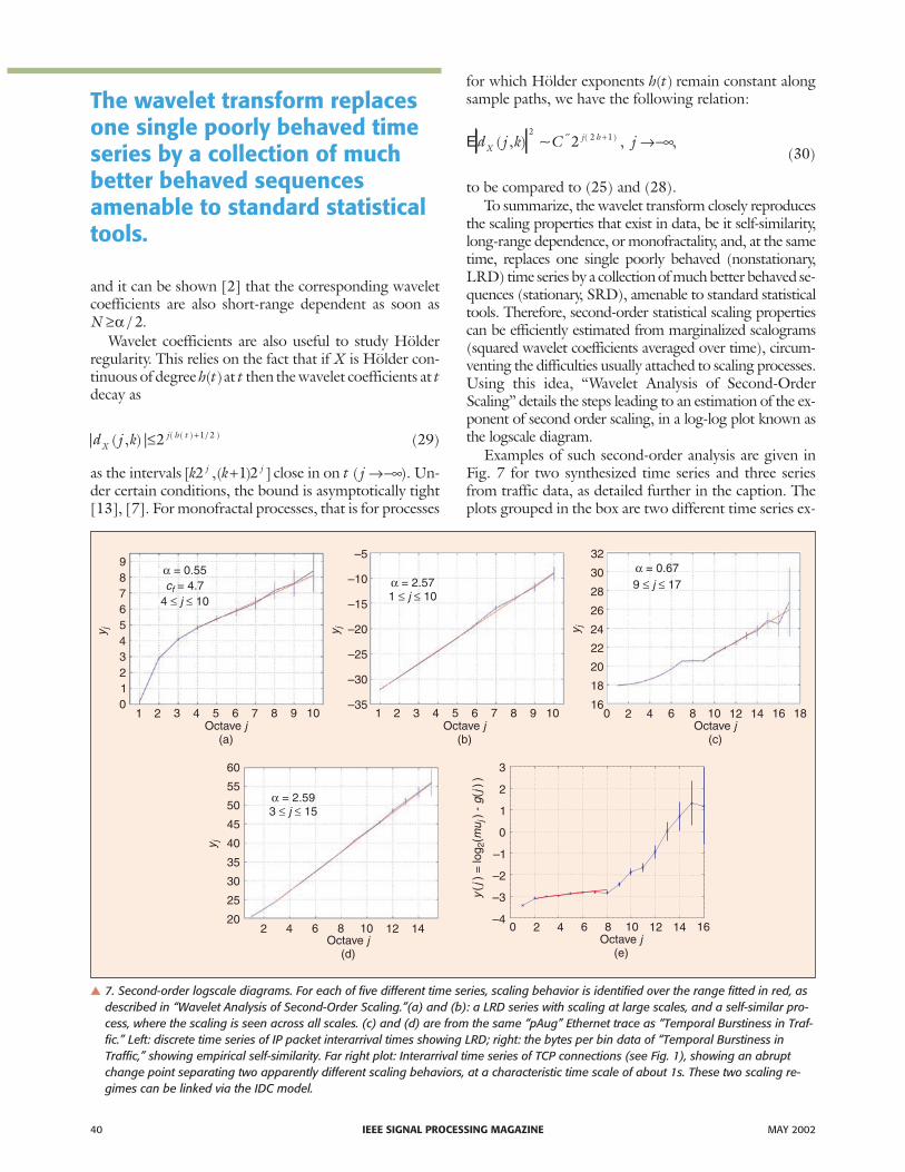
Examples of such second-order analysis are given inFig. 7 for two synthesized time series and three seriesfrom traffic data, as detailed further in the caption. Theplots grouped in the box are two different time series ex-

40 IEEE SIGNAL PROCESSING MAGAZINE MAY 2002

9876543210

y j y j

y j

y j

–5

–10

–15

–20

–25

–30

–35

32

30

28

26

24

22

20

18

16181 12 23 34 45 56 67 78 89 910 10

Octave(a)

j Octave(b)

j Octave(c)

j

Octave(d)

j Octave(e)

j

α

≤ ≤

= 0.55= 4.7

4 10c

jf

α≤ ≤= 2.57

1 10j

α≤ ≤= 2.59

3 15j

α≤ ≤= 0.67

9 17j

0

0

2

2 2

4

4 4

6

6 6

8

8 8

10

10 10

12

12 12

14

14 14

16

16

60

55

50

45

40

35

30

25

20

3

2

1

0

–1

–2

–3

–4

yj

mu

gj

()

= lo

g(

) -

() )

2j

� 7. Second-order logscale diagrams. For each of five different time series, scaling behavior is identified over the range fitted in red, asdescribed in “Wavelet Analysis of Second-Order Scaling.”(a) and (b): a LRD series with scaling at large scales, and a self-similar pro-cess, where the scaling is seen across all scales. (c) and (d) are from the same “pAug” Ethernet trace as “Temporal Burstiness in Traf-fic.” Left: discrete time series of IP packet interarrival times showing LRD; right: the bytes per bin data of “Temporal Burstiness inTraffic,” showing empirical self-similarity. Far right plot: Interarrival time series of TCP connections (see Fig. 1), showing an abruptchange point separating two apparently different scaling behaviors, at a characteristic time scale of about 1s. These two scaling re-gimes can be linked via the IDC model.

The wavelet transform replacesone single poorly behaved timeseries by a collection of muchbetter behaved sequencesamenable to standard statisticaltools.

tracted from the same celebrated Ethernet trace [14] dis-cussed in “Temporal Burstiness in Traffic.” Series fromthis trace provided one of the first clear indications oflong-range dependence in traffic. The advent of wave-let-based analysis added precision and completeness tothe study of the empirical scaling, and to the correspond-ing measurements of the Hurst parameter [3], [38], aswell as estimates of the prefactor C′ ( 28), of importancein applications. Crucially, it also helped settle controversyas to the interpretation of the discovery, by showing thatthe observed scaling in the time series was not the resultof corrupting nonstationarities, but actually corre-sponded to long-range dependencies.

The diversity of behavior in the examples of Fig. 7 il-lustrates an important advantage of a semiparametricanalysis framework, such as the wavelet approach de-scribed here. The analysis need not make any a priori as-sumption about the range of scales over which scalingmay exist. The range is rather inferred from the analysis it-self, leading to an identification of the scaling type, suchas LRD at large scales and/or multifractality at smallscales, prior to any estimation phase. Indeed, therightmost plot shows two different scaling regimes for aseries derived from Internet data, which (from a purelysecond order viewpoint) requires two independent esti-mations. In contrast, parametric methods can easily givevery misleading results if the data is not close to the as-sumed model class, making them unsuitable for the ex-ploration of real, and complex, data. The comments ofthe previous paragraph could be expressed as “robustnesswith respect to model class.” Another form of robustnessenjoyed by wavelets is their insensitivity to deterministictrends which may be superimposed onto a process of in-terest, with undesirable consequences. These include in-validating the stationarity property of the LRD processunder study or mimicking LRD correlations when addedto a short-range dependent process [1]. Wavelets are aversatile solution to this crucial issue, since they offer thepossibility of being blind to polynomial trends. Recallthat any admissible wavelet has zero mean. This is equiva-lent to having a zeroth-order vanishing moment, or inother words, to be orthogonal to constants. In fact Nvanishing moments implies that the wavelet is blind topolynomials up to order p N≤ −1. Trends which are“close” to polynomial can be effectively eliminated in thismanner [3], and the advantage of being able to do sowithout even testing for their presence is an importantone when making sense of real data, and in particularwhen trying the distinguish nonstationarity from scalingbehavior. Building on the advantages of the wavelet ap-proach, a statistical test for the constancy of a scaling ex-ponent can be defined [40] which helps resolve thisdifficult issue.

Finally, the analysis of scaling processes is often faced,and particularly so in the case of teletraffic, with enormousquantities of data, thereby requiring methods which are ef-ficient from a computational point of view. Because of

their multiresolution structure and the related ability to beimplemented as a filter bank, wavelet-based methods areassociated with fast algorithms, out performing FFT-basedcompetitors with a complexity of only O n( ) in computa-tion (compared to O n n( log( ))) and O n(log( )) in memory,for n data points. These advantages hold not only at secondorder, but more generally, including for the more advancedtypes of analysis we now discuss.

As explained earlier, scaling may involve statistics beyondsecond order, which if observed in the limit of small

MAY 2002 IEEE SIGNAL PROCESSING MAGAZINE 41

Wavelet-Based Multifractal Formalism

The wavelet-based partition function

S q d j kjk

jX

q( ) ( , )/= ∑ −2 2 , (31)

constitutes the wavelet counterpart of the traditionalpartition function (14). It can be bounded from belowby summing only over a subset of indices k, say thosefor which | ( , )|~/2 22− j

Xjhd j k . For the sake of argument

we assume that this marks the locations where theHölder regularity of the path is indeed h (compare(29)). It follows then from box-counting methods, astandard technique in fractal geometry, that the num-ber of such indices grows asymptotically at least as2− jD h( ), implying that S qj( ) grows at least as 2 j qh D h( ( ))− .Since the choice of h was arbitrary, we arrive at the as-ymptotic bound

S qjj qh D hh( ) inf ( ( ( )))≥ −2 , (32)

which is provably tight in the limit2 0j → using a steep-est descent argument. Estimating ζ( )q from the decayof estimates of the moments S qj

j q( )~ ( )2 ζ , we arrive atan asymptotic estimate

D h D h h( ) ( )** *( )≤ = ζ , (33)

where g x xy g yy*( ) inf ( ( ))= − denotes the Legendre

transform of a function g. Note that applying the trans-form twice yields the concave hull g* * of g. It is notablethat the statistically and numerically robust global esti-mator ζ provides information on the delicate localproperties captured in D h( ), which would be almostimpossible to access directly.

In practice, ζ( )q is estimated as the least squareslope of a log-log plot of the partition sum againstscale, i.e., log( ( ))S qj against log2 j . Comparing with“Wavelet Analysis of Second-Order Scaling,” this dem-onstrates quite explicitly how multifractal analysisgoes beyond second-order statistics. Fig. 8 shows ex-amples. This wavelet-based estimator can be furtherdeveloped using the wavelet maxima method [23], [4]which addresses in particular the invertibility of (29).

scales, calls for a multifractal interpretation. Multifractalanalysis provides a “finger print” of local scaling proper-ties of the paths of a process X through the multifractalspectrum D h( ), and the multifractal formalism provides apowerful approach to numerically estimating it. Just asfor second-order scaling analysis, estimates can be basedon increments of the process or time series; however,from arguments close to those developed at second order,wavelet coefficients offer themselves as an ideal alterna-tive. Notably, tuning the number of vanishing momentsof the mother wavelet allows the analysis of processeswith Hölder exponents larger than one. “Wavelet-BasedMultifractal Formalism” gives a more detailed pictures ofthis wavelet based multifractal analysis.

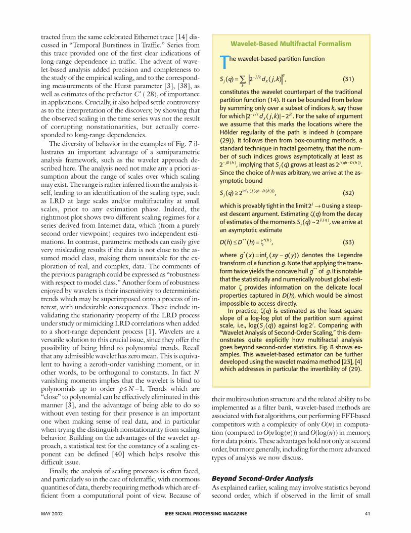
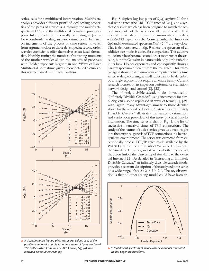
Fig. 8 depicts log-log plots of S qj ( ) against 2 j for areal-world trace (the LBL-TCP3 trace of [24]) and a syn-thetic cascade which has been designed to match the sec-ond moments of the series on all dyadic scales. It isnotable that also the sample moments of orders− ≤ ≤32 32. .q agree closely. Consequently, the functionsζ( )q and the estimated spectrum D h h( ) *( )=ζ are very close.This is demonstrated in Fig. 9 where the spectrum of anadditive tree model is added for comparison. This additivemodel matches the same second-order moments as the cas-cade, but it is Gaussian in nature with only little variationin its local Hölder exponents and consequently shows anarrow spectrum different from the real trace. This exam-ple again shows that in numerous computer network timeseries, scaling occurring at small scales cannot be describedby a single exponent but require an entire family. Currentresearch focusses on its impact on performance evaluation,network design and control [8], [28].

The infinitely divisible cascade model, introduced in“Infinitely Divisble Cascades” using increments for sim-plicity, can also be rephrased in wavelet terms [4], [39]with, again, many advantages similar to those detailedabove for the second order case. “Extracting an InfinitelyDivisible Cascade” illustrates the analysis, estimation,and verification procedure of this more practical waveletincarnation. The time series is that of Fig. 1, the list ofsuccessive interarrival times of TCP connections. Thestudy of the nature of such a series gives us direct insightinto the statistical genesis of TCP connections in a hetero-geneous environment. The series was extracted from ex-ceptionally precise TCP/IP trace made available by theWAND group at the University of Waikato. This archive,the “Auckland II” traces, are taken from both directions ofthe access link of the University of Auckland to the exter-nal Internet [22]. As detailed in “Extracting an InfinitelyDivisible Cascade,” an infinitely divisible cascade modelprovides a relevant description of the analyzed time serieson a wide range of scales: 2 2 23 14≤ ≤j . The key observa-tion is that no other scaling model could have been ap-

42 IEEE SIGNAL PROCESSING MAGAZINE MAY 2002

40

40

20

20

0

0

–20

–20

–40

–40

0

0

5

5

10

10

15

15

Scale(a)

j

Scale(b)

j

log

((

))2

Sq

jlo

g(

())

2S

qj

q = 3.2qqqq

qqqq

= 2.4= 1.6= 0.8= 0.0

= –0.8= –1.6= –2.4= –3.2

q = 3.2qqqq

qqqq

= 2.4= 1.6= 0.8= 0.0

= –0.8= –1.6= –2.4= –3.2

� 8. Superimposed log-log plots, at several values of q, of thepartition sum against scale for a time series of bytes per bin ofTCP traffic (taken from the LBL-TCP3 trace [24]) (a), and amatched binomial cascade (b).

1

0.8

0.6

0.4

0.2

Mul

tifra

ctal

Spe

ctr u

m

0.6 0.8 1 1.2 1.4Holder Exponent

Trace Data

fGn

Cascade

� 9. Multifractal spectrum of local Hölder exponents estimatedvia the Legendre transform.

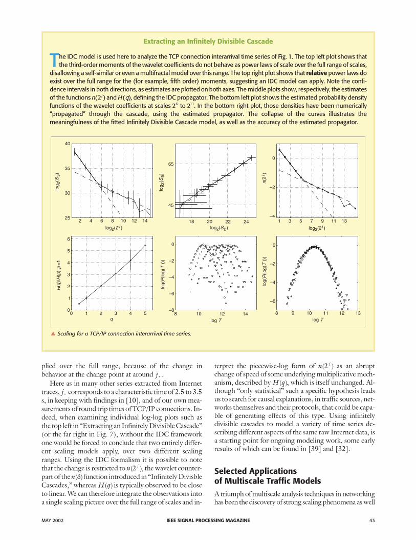
plied over the full range, because of the change inbehavior at the change point at around j* .

Here as in many other series extracted from Internettraces, j* corresponds to a characteristic time of 2.5 to 3.5s, in keeping with findings in [10], and of our own mea-surements of round trip times of TCP/IP connections. In-deed, when examining individual log-log plots such asthe top left in “Extracting an Infinitely Divisible Cascade”(or the far right in Fig. 7), without the IDC frameworkone would be forced to conclude that two entirely differ-ent scaling models apply, over two different scalingranges. Using the IDC formalism it is possible to notethat the change is restricted to n j( )2 , the wavelet counter-part of the n( )δ function introduced in “Infinitely DivisbleCascades,” whereas H q( ) is typically observed to be closeto linear. We can therefore integrate the observations intoa single scaling picture over the full range of scales and in-

terpret the piecewise-log form of n j( )2 as an abruptchange of speed of some underlying multiplicative mech-anism, described by H q( ), which is itself unchanged. Al-though “only statistical” such a specific hypothesis leadsus to search for causal explanations, in traffic sources, net-works themselves and their protocols, that could be capa-ble of generating effects of this type. Using infinitelydivisible cascades to model a variety of time series de-scribing different aspects of the same raw Internet data, isa starting point for ongoing modeling work, some earlyresults of which can be found in [39] and [32].

Selected Applicationsof Multiscale Traffic ModelsA triumph of multiscale analysis techniques in networkinghas been the discovery of strong scaling phenomena as well

MAY 2002 IEEE SIGNAL PROCESSING MAGAZINE 43

Extracting an Infinitely Divisible Cascade

The IDC model is used here to analyze the TCP connection interarrival time series of Fig. 1. The top left plot shows thatthe third-order moments of the wavelet coefficients do not behave as power laws of scale over the full range of scales,

disallowing a self-similar or even a multifractal model over this range. The top right plot shows that relative power laws doexist over the full range for the (for example, fifth order) moments, suggesting an IDC model can apply. Note the confi-dence intervals in both directions, as estimates are plotted on both axes. The middle plots show, respectively, the estimatesof the functions n j( )2 and H q( ), defining the IDC propagator. The bottom left plot shows the estimated probability densityfunctions of the wavelet coefficients at scales 26 to 211. In the bottom right plot, those densities have been numerically“propagated” through the cascade, using the estimated propagator. The collapse of the curves illustrates themeaningfulness of the fitted Infinitely Divisible Cascade model, as well as the accuracy of the estimated propagator.

40

35

30

25

log

()

2S

3

log

()

2S

5

2 4 6 8 10 12 14

log ( )2 2 j18 20 22 24

log ( )2 S2 log (2 )2j

45

65

1 3 5 7 9 11 13–4

–2

0

n(2

)j

6

5

4

3

2

1

0

Hq

Hp

p(

)/

( )

, =

1

0 1 2 3 4 5q

0

–2

–4

–6

–8

log(

(log(

)))

PT

log(

(log(

)))

PT

8 10 12 14log T

0

–2

–4

–6

8 9 10 11 12 13log T

� Scaling for a TCP/IP connection interarrival time series.

as convincing evidence pointing to causes behind it: net-working mechanisms, protocols, source characteristics,and so on. But the multiscale concept is applicable to net-work-related problems beyond the mere analysis of traffictraces. In this section, we briefly outline some applicationsthat directly leverage the multiscale framework.

Since the construction of network routers consists largelyin combining queues (buffers), queuing analysis plays acrucial role in their design and performance. In the sim-plest queuing analysis, an aggregate traffic input X t( ) isfed into a single-server queue of size B bytes with servicerate s bytes/s, and we wish to determine informationabout Q t( ), the queue size in bytes at time t. For example,we might desire the average queue size or the probabilitythat the queue will overflow, the tail queue probabilityP Q B( )> . Queuing analysis in general is extremely diffi-cult, owing to the inherent nonlinearities associated witha queue emptying (few packet arrivals) and overflowing(too many packet arrivals).

A distinct advantage of the classical Poisson trafficmodel for X t( ) is the existence of analytic formulae forP Q B( )> [17]. But the fact that real traffic is not Poissonrenders these results of limited utility in real-world situa-tions. Another approximate approach is to study only theso-called critical time scale that dominates queue overflow.

But as we have seen, real traffic is not typically domi-nated in a simple way by a single time scale. Real traffic ismultiscale, and so we should study the queue size Q t( ) atmultiple time scales and fuse the results into a single sta-tistic. A multiscale model for X t( )(such as fBm or a bino-mial cascade) facilitates the investigation of thedistribution of Q t( ) at multiple scales, incorporating thefull multiscale structure. In this framework, the distribu-tions of the wavelet coefficients of the fBm model, ormultipliers in the cascade models, are combined into asimple formula that provides a close approximation to thetail queue probability. See [27] for more details.

To understand and predict the performance ofend-to-end protocols such as TCP and modern streamingprotocols, it is crucial to understand the dynamics of theend-to-end paths through a network. In particular, wecould have interest in the delays and losses experienced bypackets transmitted end-to-end. Here we focus on delayrather than loss.

Information on packet delay can be obtained either byactively probing the path with packets or by passivelymonitoring packets as they pass a fixed point. We will fo-cus on an active strategy. The delay a packet will incur isbounded below by the “speed of light” from the transmit-ter to receiver. However, it can be considerably larger ifthere is significant cross-traffic that forces the packet towait in a buffer before it is serviced. Clearly, modelling the

end-to-end packet delay process implicitly involves mod-elling the cross-traffic, since large delays are caused bylarge traffic flows along the path.

A typical Internet end-to-end path can easily passthrough 15 or more queues, which complicates analysisand modelling considerably. Fortunately, in certain cases,an end-to-end path can be replaced by single “bottleneck”queue that is driven both by the probe traffic and an “effec-tive cross-traffic” stream that models the contributions ofall competing traffic along the path. Our fundamental ob-servation for this bottleneck queue model is as follows: thedelay spread at the receiver between two probe packetstransmitted closely spaced in time corresponds directly tothe amount of cross-traffic along the path.

Inherent in any probing scheme is an uncertainty prin-ciple, or “accuracy/sparsity tradeoff.” The volume ofcross-traffic entering the bottleneck queue between thetwo probes can be computed essentially exactly from thedelay spread of the two packets at the receiver providedthe queue does not empty in between. Unfortunately, thisemptying will certainly occur unless the probes are spacedvery closely. Even worse, long probing trains of closelyspaced packets will overwhelm the very network we aretrying to model. If the probes are spaced far apart, thenthe queue can empty in between, which results in uncer-tainty in the cross-traffic measurement.

Again, help is on the way with a multiscale model.Modeling the cross-traffic as a multiscale process (fBm orbinomial cascade for example), we can transmit a streamof packets that probes simultaneously at several timescales. For example, by spacing the packets exponentially(two packets with small spacing T followed by a packetevery2 k T , k=1,2,K), we probe the bottleneck queue at amultitude of dyadic scales.

This so-called “chirp packet train” balances the accu-racy/sparcity trade-off by being highly accurate initiallyand highly sparse at the end [28]. Packet chirps allows usto estimate the cross-traffic volume (or equivalently delaydistribution) at any dyadic scale of interest. The algo-rithm works quite well in simulation studies; currently itis under more exhaustive testing on real networks.

ConclusionsIn this article, we have seen that the complexity and rich-ness of teletraffic is well matched by the multiscale analy-sis and modeling frameworks of self-similarity,long-range dependence, fractals, multifractals, and infi-nitely divisible cascades. These frameworks not only al-low us to confirm and formalize the presence ofmultiscale behavior in traffic, but also point to possiblecauses of multiscale structure in the physical networkinginfrastructure. The choice of framework, from a simplefBm to a more complicated multifractal or cascade,clearly depends on the application and the data at hand.But whatever the framework, the multiscale wavelet

44 IEEE SIGNAL PROCESSING MAGAZINE MAY 2002

transform provides a parsimonious and efficient domainfor processing.

Finally, we note that the tools overviewed here havefound a home in numerous other areas of science and en-gineering, including turbulence and percolation, amongmany others. MATLAB routines implementing the anal-ysis/estimation procedures described throughout thistext are available at www.emulab.ee.mu.oz.au/~darryland www.dsp.rice.edu/.

AcknowledgmentsThis work was supported by grants from USA DARPA,DOE, and NSF, the French CNRS, and by Ericcson.

Patrice Abry received the degree of Professeur-Agrege deSciences Physiques in 1989 at Ecole Normale Superieurede Cachan and completed a Ph.D. in physics and signalprocessingat Ecole Normale Superieure de Lyon andUniversite Claude-Bernard Lyon I in 1994. Since 1995,he has been a permanent CNRS researcher at thelaboratoire de Physique of Ecole Normale Superieure deLyon. He received the AFCET-MESR-CNRS prize forbest Ph.D. in signal processing for the years 1993-1994and is the author of a book Ondelettes et Turbulences—Multiresolution, algorithmes de decompositions, invarianced’echelle et signaux de pression (Paris, France: Diderot,1997). His current research interests include wave-let-based analysis and modeling of scaling phenomenaand related topics.

Richard G. Baraniuk received the B.Sc. degree from theUniversity of Manitoba (Canada), the M.Sc. degree fromthe University of Wisconsin-Madison, and the Ph.D. de-gree from the University of Illinois at Urbana-Cham-paign, all in electrical engineering. After spending1992-1993 with the Signal Processing Laboratory ofEcole Normale Superieure, in Lyon, France, he joinedRice University, where he is currently a Professor of Elec-trical and Computer Engineering and DJ at KTRU. Hespent Autumn 1998 at the Isaac Newton Institute ofCambridge University, U.K., as the Rosenbaum Fellowand 2001-2002 on sabbatical at ENST in Paris and EPFLin Lausanne, Switzerland. His research interests lie in thearea of signal and image processing and include wavelets,probabilistic models, networks, and time-frequency anal-ysis. He is a Fellow of the IEEE, a member of the SignalProcessing Theory and Methods Technical Committee ofthe IEEE Signal Processing Society, and serves on the edi-torial board of the journal Applied and ComputationalHarmonic Analysis.

Patrick Flandrin is currently Directeur de Recherches atCNRS, Ecole Normale Superieure de Lyon, France. Hisresearch interests include nonstationary signal processingand the study of self-similar stochastic processes. He has

published more than 100 journal or conference papers inthese areas, contributed several chapters to collectivebooks, and authored the book Time-Frequency/Time-ScaleAnalysis (San Diego: Academic, 1999). He has beenawarded the Philip Morris Scientific Prize in Mathematicsin 1991, the SPIE Wavelet Pioneer Award in 2001, and thePrix Michel Monpetit from the French Academy of Sci-ences in 2001. He is a member of the Signal ProcessingTheory and Methods Technical Committee of the IEEESignal Processing Society and a Fellow of the IEEE.

Rudolf H. Riedi received the M.Sc. degree in 1986 and thePh.D. degree in 1993, both from the Federal Institute ofTechnology ETH Zurich (Switzerland) in mathematics.From 1993-1995 he was with the Mathematics Depart-ment of Yale University, CT, and spent 1995-1997 withthe National Research Institute in Automation and Com-puting INRIA in Paris, France. He is currently a FacultyFellow with the Electrical and Computer EngineeringDepartment at Rice University in Houston, TX. His re-search interests lie in the theory and practice ofmultifractals, multiscale analysis, and synthesis, especiallyfor network traffic. He won the ETHZ Polya prize in1986. He received a postdoctoral fellowship from theNational Science Foundation of Switzerland in 1993 anda research grant from the Centre National des Etudes enTelecommunications, France, in 1995. He served as aguest editor for the IEEE Transactions on Signal Processing.

Darryl Veitch completed a Bachelor of Science Honoursdegree at Monash University, Melbourne, in 1985 and amathematics doctorate in dynamical systems at the Uni-versity of Cambridge, U.K., in 1990. In 1991 he joinedTelecom Australia (Telstra) in Melbourne. In 1994 hejoined CNET in Paris (France Telecom). He then heldvisiting positions at the KTH, Stockholm; INRIA,France; and Bellcore, New Jersey, before taking up athree-year position as Senior Research Fellow at RMIT,Melbourne. He is now a Senior Research Fellow in theElectrical and Electronic Engineering Department at theUniversity of Melbourne. His research interests includescaling models of packet traffic, parameter estimationproblems and queueing theory for scaling processes, andthe statistical and dynamic nature of Internet traffic.

References[1] P. Abry, P. Flandrin, M.S. Taqqu, and D. Veitch, “Wavelets for the analy-

sis, estimation and synthesis of scaling data,” in Self-Similar Network Trafficand Performance Evaluation, K. Park and W. Willinger, Eds. New York:Wiley, 2000, pp. 39-88.

[2] P. Abry, P. Gonçalvès, and P. Flandrin, “Wavelets, spectrum estimationand 1/ f processes,” in Wavelets and Statistics, Lecture Notes in Statistics, A.

Antoniadis and G. Oppenheim, Eds. New York: Springer-Verlag, 1995,pp. 15-30.

[3] P. Abry and D. Veitch, “Wavelet analysis of long-range dependent traffic,”IEEE Trans. Inform. Theory, vol. 44, pp. 2-15, 1998.

MAY 2002 IEEE SIGNAL PROCESSING MAGAZINE 45

[4] A. Arnéodo, J.F. Muzy, and S.G. Roux, “Experimental analysis of self-simi-lar random cascade processes: Application to fully developed turbulence,” J.Phys. II France, vol. 7, pp. 363-370, 1997.

[5] J. Beran, Statistics for Long-Memory Processes. New York: Chapman andHall, 1994.

[6] B. Castaing, “The temperature of turbulent flows,” J. Phys. II France, vol. 6,pp. 105-114, 1996.

[7] I. Daubechies, Ten Lectures on Wavelets. New York: SIAM, 1992.

[8] A. Erramilli, O. Narayan, A. Neidhardt, and I. Saniee, “Performance im-pacts of multi-scaling in wide area TCP/IP traffic,” in Proc. IEEEInfocom’2000, Tel Aviv, Israel, Mar. 2000, pp. 352-359.

[9] K. Falconer, Fractal Geometry—Mathematical Foundations and Applications.New York: Wiley, 1990.

[10] A. Feldmann, A.C. Gilbert, P. Huang, and W. Willinger, “Dynamics of IPtraffic, A study of the role of variability and the impact of control,” in Proc.ACM/Sigcomm’99, Cambridge, MA, Aug. 1999, pp. 301-313.

[11] P. Flandrin, “Wavelet analysis and synthesis of fractional Brownian mo-tion,” IEEE Trans. Inform. Theory, vol. 38, pp. 910-917, 1992.

[12] A.C. Gilbert, “Multiscale analysis and data networks,” Appl. Comp.Harmon. Anal., vol. 10, no. 3, pp. 185-202, 2001.

[13] S. Jaffard, “Local behavior of Riemann’s function,” Contemporary Mathe-matics, vol. 189, pp. 287-307, 1995.

[14] W.E. Leland, M.S. Taqqu, W. Willinger, and D.V. Wilson, “On theself-similar nature of Ethernet traffic,” Comput. Commun. Rev., vol. 23, pp.183-193, 1993.

[15] W.E. Leland and D.V. Wilson, “High time-resolution measurement andanalysis of lan traffic: Implications for lan interconnection,” in Proc. IEEEInfocom’91, Bal Harbour, FL, 1991, pp. 1360-1366.

[16] J. Lévy-Véhel and R. Riedi, “Fractional Brownian motion and data trafficmodeling: The other end of the spectrum,” in Fractals in Engineering, J.Lévy-Véhel, E. Lutton, and C. Tricot, Eds. London, U.K.:Springer-Verlag, 1997, pp. 185-203.

[17] D.V. Lindley, “The theory of queues with a single server,” Proc. Cam-bridge Phil. Soc., vol. 48, pp. 277-289, 1952.

[18] S. Mallat, A Wavelet Tour of Signal Processing. Boston, MA: Academic, 1997.

[19] B.B. Mandelbrot and J.W. Van Ness, “Fractional Brownian motions, frac-tional noises and applications,” SIAM Rev., vol. 10, pp. 422-437, 1968.

[20] P. Mannersolo, I. Norros, and R. Riedi, “Multifractal products of stochas-tic processes: Construction and some basic properties,” COST (EuropeanCooperation in the field of Scientific and Technical Research) 257, Tech.Rep., COST257TD(99)31, 1999.

[21] K. Meier-Hellstern, P.E. Wirth, Y.-L. Yan, and D.A. Hoeflin, “Trafficmodels for ISDN data users: Office automation application,” in Proc. 13thITC, Copenhagen, Denmark, 1991, pp. 167-172.

[22] J. Micheel, I. Graham, and N. Brownlee, “The Auckland data set: An ac-cess link observed,” in Proc. 14th ITC Specialist Seminar, Barcelona, Spain,April 2000.

[23] J.F. Muzy, E. Bacry, and A. Arnéodo, “The multifractal formalism revis-ited with wavelets,” Int. F. Bifur. Chaos, vol. 4, no. 2, pp. 245-301, 1994.

[24] V. Paxson and S. Floyd, “Wide-area traffic: The failure of Poisson model-ing,” IEEE/ACM Trans. Networking, vol. 3, pp. 226-244, 1995.

[25] R.F. Peltier and J. Lévy-Véhel, “Multifractional Brownian motion: Defi-nition and preliminary results”, INRIA, Rocquencourt, France, Res. Rep.No. 2645, 1995.

[26] K. Park and W. Willinger, Eds., Self-Similar Network Traffic and Perfor-mance Evaluation. New York: Wiley, 2000.

[27] V. Ribeiro, R. Riedi, M.S. Crouse, and R. Baraniuk, “Multiscale queuinganalysis of long-range-dependent network traffic,” Proc. IEEE Infocomm.,vol. 2, pp. 1026-1035, Mar. 2000. Available: dsp.rice.edu.

[28] V. Ribeiro, M. Coates, R. Riedi, S. Sarvotham, B. Hendricks, and R.Baraniuk, “Multifractal cross-traffic estimation,” in Proc. ITC Specialist Semi-nar on IP Traffic Measurement, Modeling, and Management, Monterey, CA,Sept. 2000, pp. 15-1 - 15-10. Available: dsp.rice.edu.

[29] R. Riedi, “An improved multifractal formalism and self-similar measures,”J. Math. Anal. Appl., vol. 189, pp. 462-490, 1995.

[30] R. Riedi, M.S. Crouse, V.J. Ribeiro, and R.G. Baraniuk, “A multifractalwavelet model with application to network traffic,” IEEE Trans. Inform.Theory (Special Issue), vol. 45, no. 3, pp. 992-1018, Apr. 1999.

[31] R. Riedi, “Multifractal processes,” in Long Range Dependence: Theory andApplications, Doukhan, Oppenheim and Taqqu, Eds. to appear.

[32] S. Roux, D. Veitch, P. Abry, L. Huang, P. Flandrin, and J. Micheel, “Sta-tistical scaling analysis of TCP/IP data,” in Proc. ICASSP 2001, Special Ses-sion, Network Inference and Traffic Modeling, Salt Lake City, UT, May 2001.

[33] G. Samorodnitsky and M.S. Taqqu, Stable Non-Gaussian Processes: Stochas-tic Models with Infinite Variance. New York: Chapman & Hall, 1994.

[34] M.S. Taqqu, V. Teverovsky, and W. Willinger, “Estimators forlong-range dependence: An empirical study,” Fractals, vol. 3, no. 4, pp.785-798, 1995.

[35] M.S. Taqqu, V. Teverovsky, and W. Willinger, “Is network trafficself-similar or multifractal?,” Fractals, vol. 5, pp. 63-74, 1997.

[36] M.S. Taqqu, W. Willinger, and R. Sherman, “Proof of a fundamental re-sult in self-similar traffic modeling,” Comput. Commun. Rev., vol. 26, pp.5-23, 1997.

[37] A.H. Tewfik and M. Kim, “Correlation structure of the discrete waveletcoefficients of fractional Brownian motion,” IEEE Trans. Inform. Theory,vol. 38, pp. 904-909, 1992.

[38] D. Veitch and P. Abry, “A wavelet-based joint estimator for the parame-ters of long-range dependence,” IEEE Trans. Inform. Theory, vol. 45, no. 3,pp. 878-897, 1999.

[39] D. Veitch, P. Abry, P. Flandrin, and P. Chainais, “Infinitely divisible cas-cade analysis of network traffic data,” in Proc. ICASSP 2000, Istanbul, Tur-key, June 2000.

[40] D. Veitch and P. Abry, “A statistical test for the time constancy of scaling ex-ponents,” IEEE Trans. Signal Processing, vol. 49, pp. 2325-2334, Oct. 2001.

46 IEEE SIGNAL PROCESSING MAGAZINE MAY 2002