Embed Size (px)
Citation preview
On the Number of Linear Regions ofDeep Neural Networks
Guido MontufarMax Planck Institute for Mathematics in the Sciences
Razvan PascanuUniversite de Montreal
Kyunghyun ChoUniversite de Montreal
Yoshua BengioUniversite de Montreal, CIFAR [email protected]
Abstract
We study the complexity of functions computable by deep feedforward neural net-works with piecewise linear activations in terms of the symmetries and the numberof linear regions that they have. Deep networks are able to sequentially map por-tions of each layer’s input-space to the same output. In this way, deep modelscompute functions that react equally to complicated patterns of different inputs.The compositional structure of these functions enables them to re-use pieces ofcomputation exponentially often in terms of the network’s depth. This paper inves-tigates the complexity of such compositional maps and contributes new theoreticalresults regarding the advantage of depth for neural networks with piecewise linearactivation functions. In particular, our analysis is not specific to a single family ofmodels, and as an example, we employ it for rectifier and maxout networks. Weimprove complexity bounds from pre-existing work and investigate the behaviorof units in higher layers.Keywords: Deep learning, neural network, input space partition, rectifier, maxout
1 Introduction
Artificial neural networks with several hidden layers, called deep neural networks, have become pop-ular due to their unprecedented success in a variety of machine learning tasks (see, e.g., Krizhevskyet al. 2012, Ciresan et al. 2012, Goodfellow et al. 2013, Hinton et al. 2012). In view of this empiri-cal evidence, deep neural networks are becoming increasingly favoured over shallow networks (i.e.,with a single layer of hidden units), and are often implemented with more than five layers. At thetime being, however, only a limited amount of publications have investigated deep networks froma theoretical perspective. Recently, Delalleau and Bengio (2011) showed that a shallow networkrequires exponentially many more sum-product hidden units1 than a deep sum-product network inorder to compute certain families of polynomials. We are interested in extending this kind of analysisto more popular neural networks.
There is a wealth of literature discussing approximation, estimation, and complexity of artificial neu-ral networks (see, e.g., Anthony and Bartlett 1999). A well-known result states that a feedforwardneural network with a single, huge, hidden layer is a universal approximator of Borel measurablefunctions (see Hornik et al. 1989, Cybenko 1989). Other works have investigated universal approx-imation of probability distributions by deep belief networks (Le Roux and Bengio 2010, Montufarand Ay 2011), as well as their approximation properties (Montufar 2014, Krause et al. 2013).
1A single sum-product hidden layer summarizes a layer of product units followed by a layer of sum units.
1
arX
iv:1
402.
1869
v2 [
stat
.ML
] 7
Jun
201
4
2.0 1.5 1.0 0.5 0.0 0.5 1.0 1.5 2.02.0
1.5
1.0
0.5
0.0
0.5
1.0
1.5
2.0
2.0 1.5 1.0 0.5 0.0 0.5 1.0 1.5 2.02.0
1.5
1.0
0.5
0.0
0.5
1.0
1.5
2.0
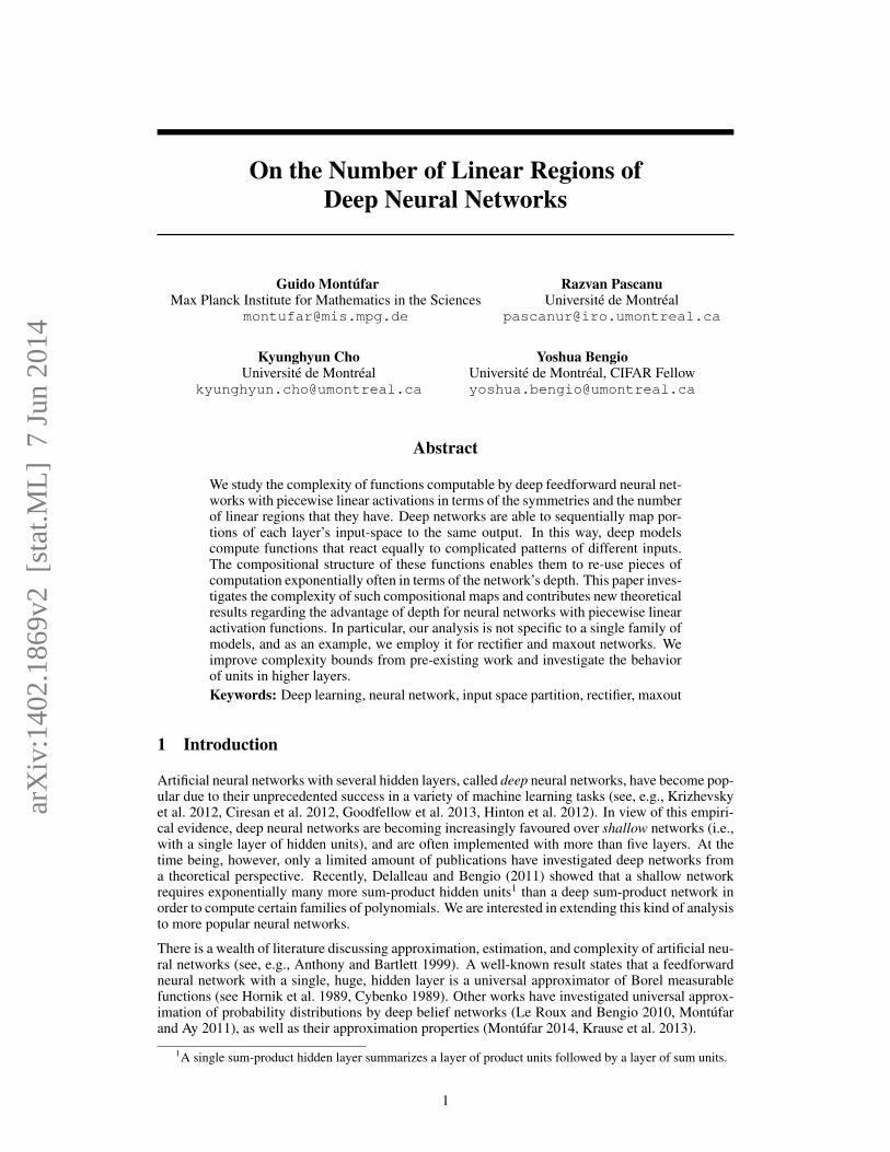
Figure 1: Binary classification using a shallow model with 20 hidden units (solid line) and a deepmodel with two layers of 10 units each (dashed line). The right panel shows a close-up of the leftpanel. Filled markers indicate errors made by the shallow model.
These previous theoretical results, however, do not trivially apply to the types of deep neural net-works that have seen success in recent years. Conventional neural networks often employ eitherhidden units with a bounded smooth activation function, or Boolean hidden units. On the otherhand, recently it has become more common to use piecewise linear functions, such as the rectifieractivation g(a) = max0, a (Glorot et al. 2011, Nair and Hinton 2010) or the maxout activationg(a1, . . . , ak) = maxa1, . . . , ak (Goodfellow et al. 2013). The practical success of deep neuralnetworks with piecewise linear units calls for the theoretical analysis specific for this type of neuralnetworks.
In this respect, Pascanu et al. (2013) reported a theoretical result on the complexity of functionscomputable by deep feedforward networks with rectifier units. They showed that, in the asymptoticlimit of many hidden layers, deep networks are able to separate their input space into exponentiallymore linear response regions than their shallow counterparts, despite using the same number ofcomputational units.
Building on the ideas from (Pascanu et al. 2013), we develop a general framework for analyzingdeep models with piecewise linear activations. The intermediary layers of these models are able tomap several pieces of their inputs into the same output. The layer-wise composition of the functionscomputed in this way re-uses low-level computations exponentially often as the number of layersincreases. This key property enables deep networks to compute highly complex and structuredfunctions. We underpin this idea by estimating the number of linear regions of functions computableby two important types of piecewise linear networks: with rectifier units and with maxout units.
Our results for the complexity of deep rectifier networks yield a significant improvement over theprevious results on rectifier networks mentioned above, showing a favourable behavior of deep overshallow networks even with a moderate number of hidden layers. Our analysis of deep rectifier andmaxout networks serves as plattform to study a broad variety of related networks, such as convolu-tional networks.
The number of linear regions of the functions that can be computed by a given model is a measureof the model’s flexibility. An example of this is given in Fig. 1, which compares the learnt deci-sion boundary of a single-layer and a two-layer model with the same number of hidden units (seedetails in Appendix F). This illustrates the advantage of depth; the deep model captures the desiredboundary more accurately, approximating it with a larger number of linear pieces.
As noted earlier, deep networks are able to identify an exponential number of input neighborhoods bymapping them to a common output of some intermediary hidden layer. The computations carried outon the activations of this intermediary layer are replicated many times, once in each of the identifiedneighborhoods. This allows the networks to compute very complex looking functions even whenthey are defined with relatively few parameters.
The number of parameters is an upper bound for the dimension of the set of functions computableby a network, and a small number of parameters means that the class of computable functions hasa low dimension. The set of functions computable by a deep feedforward piecewise linear network,although low dimensional, achieves exponential complexity by re-using and composing featuresfrom layer to layer.
2

2 Feedforward Neural Networks and their Compositional Properties
In this section we discuss the ability of deep feedforward networks to re-map their input-space tocreate complex symmetries by using only relatively few computational units. The key observationof our analysis is that each layer of a deep model is able to map different regions of its input toa common output. This leads to a compositional structure, where computations on higher layersare effectively replicated in all input regions that produced the same output at a given layer. Thecapacity to replicate computations over the input-space grows exponentially with the number ofnetwork layers. Before expanding these ideas, we introduce basic definitions needed in the restof the paper. At the end of this section, we give an intuitive perspective for reasoning about thereplicative capacity of deep models.
2.1 Definitions
A feedforward neural network is a composition of layers of computational units which defines afunction F : Rn0 → Rout of the form
F (x; θ) = fout gL fL · · · g1 f1(x), (1)
where fl is a linear pre-activation function and gl is a nonlinear activation function. The parameter θis composed of input weight matrices Wl ∈ Rk·nl×nl−1 and bias vectors bl ∈ Rk·nl for each layerl ∈ [L].
The output of the l-th layer is a vector xl = [xl,1, . . . ,xl,nl]> of activations xl,i of the units i ∈ [nl]
in that layer. This is computed from the activations of the preceding layer by xl = gl(fl(xl−1)).Given the activations xl−1 of the units in the (l− 1)-th layer, the pre-activation of layer l is given by
fl(xl−1) = Wlxl−1 + bl,
where fl = [fl,1, . . . , fl,nl]> is an array composed of nl pre-activation vectors fl,i ∈ Rk, and the
activation of the i-th unit in the l-th layer is given by
xl,i = gl,i(fl,i(xl−1)).
We will abbreviate gl fl by hl. When the layer index l is clear, we will drop the correspondingsubscript. We are interested in piecewise linear activations, and will consider the following twoimportant types.
• Rectifier unit: gi(fi) = max 0, fi, where fi ∈ R and k = 1.• Rank-k maxout unit: gi(fi) = maxfi,1, . . . , fi,k, where fi = [fi,1, . . . , fi,k] ∈ Rk.
The structure of the network refers to the way its units are arranged. It is specified by the numbern0 of input dimensions, the number of layers L, and the number of units or width nl of each layer.
We will classify the functions computed by different network structures, for different choices ofparameters, in terms of their number of linear regions. A linear region of a piecewise linear functionF : Rn0 → Rm is a maximal connected subset of the input-space Rn0 , on which F is linear. For thefunctions that we consider, each linear region has full dimension, n0.
2.2 Shallow Neural Networks
Rectifier units have two types of behavior; they can be either constant 0 or linear, depending on theirinputs. The boundary between these two behaviors is given by a hyperplane, and the collection ofall the hyperplanes coming from all units in a rectifier layer forms a hyperplane arrangement. Ingeneral, if the activation function g : R → R has a distinguished (i.e., irregular) behavior at zero(e.g., an inflection point or non-linearity), then the function Rn0 → Rn1 ; x 7→ g(Wx + b) has adistinguished behavior at all inputs from any of the hyperplanes Hi := x ∈ Rn0 : Wi,:x + bi =0 for i ∈ [n1]. The hyperplanes capturing this distinguished behavior also form a hyperplanearrangement.
The hyperplanes in the arrangement split the input-space into several regions. Formally, a region of ahyperplane arrangement H1, . . . ,Hn1 is a connected component of the complement Rn0\(∪iHi),
3
i.e., a set of points delimited by these hyperplanes (possibly open towards infinity). The number ofregions of an arrangement can be given in terms of a characteristic function of the arrangement,as shown in a well-known result by Zaslavsky (1975). An arrangement of n1 hyperplanes in Rn0
has at most∑n0
j=0
(n1
j
)regions. Furthermore, this number of regions is attained if and only if the
hyperplanes are in general position. This implies that the maximal number of linear regions offunctions computed by a shallow rectifier network with n0 inputs and n1 hidden units is
∑n0
j=0
(n1
j
)(see Pascanu et al. 2013; Proposition 5).
2.3 Deep Neural Networks
We start by defining the identification of input neighborhoods mentioned in the introduction moreformally:
Definition 1. A map F identifies two neighborhoods S and T of its input domain if it maps themto a common subset F (S) = F (T ) of its output domain. In this case we also say that S and T areidentified by F .
For example, the four quadrants of 2-D Euclidean space are regions that are identified by the absolutevalue function g : R2 → R2;
g(x1, x2) = [|x1| , |x2|]> . (2)
The computation carried out by the l-th layer of a feedforward network on a set of activations fromthe (l − 1)-th layer is effectively carried out for all regions of the input space that lead to the sameactivations of the (l − 1)-th layer. One can choose the input weights and biases of a given layerin such a way that the computed function behaves most interestingly on those activation values ofthe preceding layer which have the largest number of preimages in the input space, thus replicatingthe interesting computation many times in the input space and generating an overall complicated-looking function.
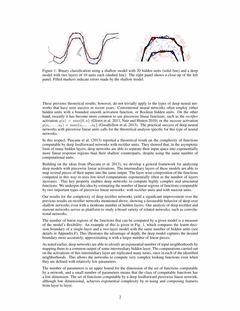
For any given choice of the network parameters, each hidden layer l computes a function hl = glflon the output activations of the preceding layer. We consider the function Fl : Rn0 → Rnl ; Fl :=hl · · · h1 that computes the activations of the l-th hidden layer. We denote the image of Fl bySl ⊆ Rnl , i.e., the set of (vector valued) activations reachable by the l-th layer for all possible inputs.Given a subset R ⊆ Sl, we denote by P lR the set of subsets R1, . . . , Rk ⊆ Sl−1 that are mapped byhl onto R; that is, subsets that satisfy hl(R1) = · · · = hl(Rk) = R. See Fig. 2 for an illustration.
The number of separate input-space neighborhoods that are mapped to a common neighborhoodR ⊆ Sl ⊆ Rnl can be given recursively as
N lR =
∑R′∈P l
R
N l−1R′ , N 0
R = 1, for each region R ⊆ Rn0 . (3)
For example, P 1R is the set of all disjoint input-space neighborhoods whose image by the function
computed by the first layer, h1 : x 7→ g(Wx + b), equals R ⊆ S1 ⊆ Rn1 .
The recursive formula (3) counts the number of identified sets by moving along the branches of atree rooted at the set R of the j-th layer’s output-space (see Fig. 2 (c)). Based on these observations,we can estimate the maximal number of linear regions as follows.
Lemma 2. The maximal number of linear regions of the functions computed by an L-layer neuralnetwork with piecewise linear activations is at least N =
∑R∈PL NL−1
R , where NL−1R is defined
by Eq. (3), and PL is a set of neighbordhoods in distinct linear regions of the function computed bythe last hidden layer.
Here, the idea to construct a function with many linear regions is to use the first L− 1 hidden layersto identify many input-space neighborhoods, mapping all of them to the activation neighborhoodsPL of the (L−1)-th hidden layer, each of which belongs to a distinct linear region of the last hiddenlayer.
We will give the detailed analysis of rectifier and maxout networks in Secs. 3 and 4.
4
1. Fold along the 2. Fold along thehorizontal axisvertical axis
3.
(a)
S1S2S3
S4
S ′4 S ′
1
S ′1S ′
1
S ′1 S ′
4
S ′4S ′
4
S ′2
S ′2S ′
2
S ′2 S
′3 S ′
3
S ′3 S ′
3
S ′1S ′
4
S ′2S ′
3
Input Space
First Layer Space
Second LayerSpace
(b) (c)
Figure 2: (a) Space folding of 2-D Euclidean space along the two axes. (b) An illustration of how thetop-level partitioning (on the right) is replicated to the original input space (left). (c) Identificationof regions across the layers of a deep model.
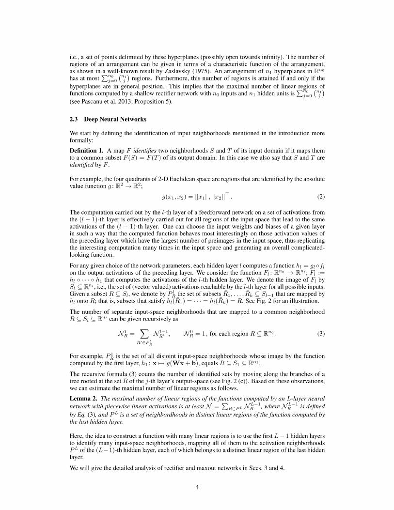
Figure 3: Space folding of 2-D space in a non-trivial way. Note how the folding can potentiallyidentify symmetries in the boundary that it needs to learn.
2.4 Identification of Inputs as Space Foldings
In this section, we discuss an intuition behind Lemma 2 in terms of space folding. A map F thatidentifies two subsets S and S ′ can be considered as an operator that folds its domain in such a waythat the two subsets S and S ′ coincide and are mapped to the same output. For instance, the absolutevalue function g : R2 → R2 from Eq. (2) folds its domain twice (once along each coordinate axis),as illustrated in Fig. 2 (a). This folding identifies the four quadrants of 2-D Euclidean space. Bycomposing such operations, the same kind of map can be applied again to the output, in order tore-fold the first folding.
Each hidden layer of a deep neural network can be associated with a folding operator. Each hiddenlayer folds the space of activations of the previous layer. In turn, a deep neural network effectivelyfolds its input-space recursively, starting with the first layer. The consequence of this recursivefolding is that any function computed on the final folded space will apply to all the collapsed subsetsidentified by the map corresponding to the succession of foldings. This means that in a deep modelany partitioning of the last layer’s image-space is replicated in all input-space regions which areidentified by the succession of foldings. Fig. 2 (b) offers an illustration of this replication property.
Space foldings are not restricted to foldings along coordinate axes and they do not have to preservelengths. Instead, the space is folded depending on the orientations and shifts encoded in the inputweights W and biases b and on the nonlinear activation function used at each hidden layer. Inparticular, this means that the sizes and orientations of identified input-space regions may differfrom each other. See Fig. 3.
2.5 Stability to Perturbation
Our bounds on the complexity attainable by deep models (Secs. 3 and 4) are based on suitablechoices of the network weights. However, this does not mean that the indicated complexity is onlyattainable in singular cases.
5
The parametrization of the functions computed by a neural network is continuous. More precisely,the map ψ : RN → C(Rn0 ;RnL); θ 7→ Fθ, which maps input weights and biases θ = Wi,biLi=1to the continuous functions Fθ : Rn0 → RnL computed by the network, is continuous. Our analysisconsiders the number of linear regions of the functions Fθ. By definition, each linear region containsan open neighborhood of the input-space Rn0 . Given any function Fθ with a finite number of linearregions, there is an ε > 0 such that for each ε-perturbation of the parameter θ, the resulting functionFθ+ε has at least as many linear regions as Fθ. The linear regions of Fθ are preserved under smallperturbations of the parameters, because they have a finite volume.
If we define a probability density on the space of parameters, what is the probability of the eventthat the function represented by the network has a given number of linear regions? By the above dis-cussion, the probability of getting a number of regions at least as large as the number resulting fromany particular choice of parameters (for a uniform measure within a bounded domain) is nonzero,even though it may be very small. This is because there exists an epsilon-ball of non-zero volumearound that particular choice of parameters, for which at least the same number of linear regions isattained.
For future work it would be interesting to study the partitions of parameter space RN into pieceswhere the resulting functions partition their input-spaces into isomorphic linear regions, and to in-vestigate how many of these pieces of parameter space correspond to functions with a given numberof linear regions.
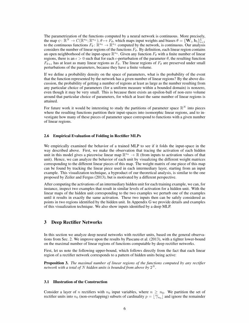
2.6 Empirical Evaluation of Folding in Rectifier MLPs
We empirically examined the behavior of a trained MLP to see if it folds the input-space in theway described above. First, we make the observation that tracing the activation of each hiddenunit in this model gives a piecewise linear map Rn0 → R (from inputs to activation values of thatunit). Hence, we can analyze the behavior of each unit by visualizing the different weight matricescorresponding to the different linear pieces of this map. The weight matrix of one piece of this mapcan be found by tracking the linear piece used in each intermediary layer, starting from an inputexample. This visualization technique, a byproduct of our theoretical analysis, is similar to the oneproposed by Zeiler and Fergus (2013), but is motivated by a different perspective.
After computing the activations of an intermediary hidden unit for each training example, we can, forinstance, inspect two examples that result in similar levels of activation for a hidden unit. With thelinear maps of the hidden unit corresponding to the two examples we perturb one of the examplesuntil it results in exactly the same activation. These two inputs then can be safely considered aspoints in two regions identified by the hidden unit. In Appendix G we provide details and examplesof this visualization technique. We also show inputs identified by a deep MLP.
3 Deep Rectifier Networks
In this section we analyze deep neural networks with rectifier units, based on the general observa-tions from Sec. 2. We improve upon the results by Pascanu et al. (2013), with a tighter lower-boundon the maximal number of linear regions of functions computable by deep rectifier networks.
First, let us note the following upper-bound, which follows directly from the fact that each linearregion of a rectifier network corresponds to a pattern of hidden units being active:
Proposition 3. The maximal number of linear regions of the functions computed by any rectifiernetwork with a total of N hidden units is bounded from above by 2N .
3.1 Illustration of the Construction
Consider a layer of n rectifiers with n0 input variables, where n ≥ n0. We partition the set ofrectifier units into n0 (non-overlapping) subsets of cardinality p = bn/n0c and ignore the remainder
6
0 1 2
1
23
h1
h2 h3
h1 − h2
h1 − h2 + h3
x
h(x)
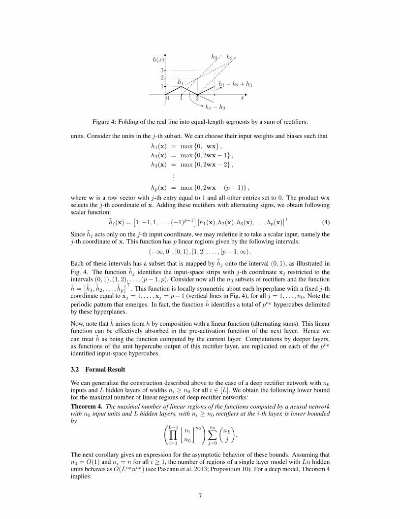
Figure 4: Folding of the real line into equal-length segments by a sum of rectifiers.
units. Consider the units in the j-th subset. We can choose their input weights and biases such that
h1(x) = max 0, wx ,h2(x) = max 0, 2wx− 1 ,h3(x) = max 0, 2wx− 2 ,
...hp(x) = max 0, 2wx− (p− 1) ,
where w is a row vector with j-th entry equal to 1 and all other entries set to 0. The product wxselects the j-th coordinate of x. Adding these rectifiers with alternating signs, we obtain followingscalar function:
hj(x) =[1,−1, 1, . . . , (−1)p−1
][h1(x), h2(x), h3(x), . . . , hp(x)]
>. (4)
Since hj acts only on the j-th input coordinate, we may redefine it to take a scalar input, namely thej-th coordinate of x. This function has p linear regions given by the following intervals:
(−∞, 0] , [0, 1] , [1, 2] , . . . , [p− 1,∞) .
Each of these intervals has a subset that is mapped by hj onto the interval (0, 1), as illustrated inFig. 4. The function hj identifies the input-space strips with j-th coordinate xj restricted to theintervals (0, 1), (1, 2), . . . , (p− 1, p). Consider now all the n0 subsets of rectifiers and the functionh =
[h1, h2, . . . , hp
]>. This function is locally symmetric about each hyperplane with a fixed j-th
coordinate equal to xj = 1, . . . ,xj = p− 1 (vertical lines in Fig. 4), for all j = 1, . . . , n0. Note theperiodic pattern that emerges. In fact, the function h identifies a total of pn0 hypercubes delimitedby these hyperplanes.
Now, note that h arises from h by composition with a linear function (alternating sums). This linearfunction can be effectively absorbed in the pre-activation function of the next layer. Hence wecan treat h as being the function computed by the current layer. Computations by deeper layers,as functions of the unit hypercube output of this rectifier layer, are replicated on each of the pn0
identified input-space hypercubes.
3.2 Formal Result
We can generalize the construction described above to the case of a deep rectifier network with n0inputs and L hidden layers of widths ni ≥ n0 for all i ∈ [L]. We obtain the following lower boundfor the maximal number of linear regions of deep rectifier networks:Theorem 4. The maximal number of linear regions of the functions computed by a neural networkwith n0 input units and L hidden layers, with ni ≥ n0 rectifiers at the i-th layer, is lower boundedby (
L−1∏i=1
⌊nin0
⌋n0)
n0∑j=0
(nLj
).
The next corollary gives an expression for the asymptotic behavior of these bounds. Assuming thatn0 = O(1) and ni = n for all i ≥ 1, the number of regions of a single layer model with Ln hiddenunits behaves asO(Ln0nn0) (see Pascanu et al. 2013; Proposition 10). For a deep model, Theorem 4implies:
7
Corollary 5. A rectifier neural network with n0 input units and L hidden layers of width n ≥ n0
can compute functions that have Ω(
(n/n0)(L−1)n0 nn0
)linear regions.
Thus we see that the number of linear regions of deep models grows exponentially in L and poly-nomially in n, which is much faster than that of shallow models with nL hidden units. Our resultis a significant improvement over the bound Ω
((n/n0
)L−1
nn0
)obtained by Pascanu et al. (2013).
In particular, our result demonstrates that even for small values of L and n, deep rectifier modelsare able to produce substantially more linear regions than shallow rectifier models. Additionally,using the same strategy as Pascanu et al. (2013), our result can be reformulated in terms of the num-ber of linear regions per parameter. This results in a similar behaviour, with deep models beingexponentially more efficient than shallow models (see Appendix C).
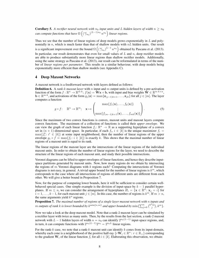
4 Deep Maxout Networks
A maxout network is a feedforward network with layers defined as follows:Definition 6. A rank-k maxout layer with n input and m output units is defined by a pre-activationfunction of the form f : Rn → Rm·k; f(x) = Wx+b, with input and bias weights W ∈ Rm·k×n,b ∈ Rm·k, and activations of the form gj(z) = maxz(j−1)k+1, . . . , zjk for all j ∈ [m]. The layercomputes a function
g f : Rn → Rm; x 7→
maxf1(x), . . . , fk(x)...
maxf(m−1)k+1(x), . . . , fmk(x)
. (5)
Since the maximum of two convex functions is convex, maxout units and maxout layers computeconvex functions. The maximum of a collection of functions is called their upper envelope. Wecan view the graph of each linear function fi : Rn → R as a supporting hyperplane of a convexset in (n + 1)-dimensional space. In particular, if each fi, i ∈ [k] is the unique maximizer fi =maxf ′i : i′ ∈ [k] at some input neighborhood, then the number of linear regions of the upperenvelope g1 f = maxfi : i ∈ [k] is exactly k. This shows that the maximal number of linearregions of a maxout unit is equal to its rank.
The linear regions of the maxout layer are the intersections of the linear regions of the individualmaxout units. In order to obtain the number of linear regions for the layer, we need to describe thestructure of the linear regions of each maxout unit, and study their possible intersections.
Voronoi diagrams can be lifted to upper envelopes of linear functions, and hence they describe input-space partitions generated by maxout units. Now, how many regions do we obtain by intersectingthe regions of m Voronoi diagrams with k regions each? Computing the intersections of Voronoidiagrams is not easy, in general. A trivial upper bound for the number of linear regions is km, whichcorresponds to the case where all intersections of regions of different units are different from eachother. We will give a better bound in Proposition 7.
Now, for the purpose of computing lower bounds, here it will be sufficient to consider certain well-behaved special cases. One simple example is the division of input-space by k − 1 parallel hyper-planes. If m ≤ n, we can consider the arrangement of hyperplanes Hi = x ∈ Rn : xj = i fori = 1, . . . , k−1, for each maxout unit j ∈ [m]. In this case, the number of regions is km. If m > n,the same arguments yield kn regions.Proposition 7. The maximal number of regions of a single layer maxout network with n inputs andm outputs of rank k is lower bounded by kminn,m and upper bounded by min∑n
j=0
(k2mj
), km.
Now we take a look at the deep maxout model. Note that a rank-2 maxout layer can be simulated bya rectifier layer with twice as many units. Then, by the results from the last section, a rank-2 maxoutnetwork with L− 1 hidden layers of width n = n0 can identify 2n0(L−1) input-space regions, and,in turn, it can compute functions with 2n0(L−1)2n0 = 2n0L linear regions.
For the rank-k case, we note that a rank-k maxout unit can identify k cones from its input-domain,whereby each cone is a neighborhood of the positive half-ray rWi ∈ Rn : r ∈ R+ correspondingto the gradient Wi of the linear function fi for all i ∈ [k]. Elaborating this observation, we obtain:
8
Theorem 8. A maxout network with L layers of width n0 and rank k can compute functions with atleast kL−1kn0 linear regions.
Theorem 8 and Proposition 7 show that deep maxout networks can compute functions with a numberof linear regions that grows exponentially with the number of layers, and exponentially faster thanthe maximal number of regions of shallow models with the same number of units. Similarly tothe rectifier model, this exponential behavior can also be established with respect to the number ofnetwork parameters.
We note that although certain functions that can be computed by maxout layers can also be com-puted by rectifier layers, the rectifier construction from last section leads to functions that are notcomputable by maxout networks (except in the rank-2 case). The proof of Theorem 8 is based onthe same general arguments from Sec. 2, but uses a different construction than Theorem 4 (detailsin Appendix D).
5 Conclusions and Outlook
We studied the complexity of functions computable by deep feedforward neural networks in termsof their number of linear regions. We specifically focused on deep neural networks having piece-wise linear hidden units which have been found to provide superior performance in many machinelearning applications recently. We discussed the idea that each layer of a deep model is able toidentify pieces of its input in such a way that the composition of layers identifies an exponentialnumber of input regions. This results in exponentially replicating the complexity of the functionscomputed in the higher layers of the model. The functions computed in this way by deep models arecomplicated, but still they have an intrinsic rigidity caused by the replications, which may help deepmodels generalize to unseen samples better than shallow models.
This framework is applicable to any neural network that has a piecewise linear activation func-tion. For example, if we consider a convolutional network with rectifier units, as the one used in(Krizhevsky et al. 2012), we can see that the convolution followed by max pooling at each layeridentifies all patches of the input within a pooling region. This will let such a deep convolutionalneural network recursively identify patches of the images of lower layers, resulting in exponentiallymany linear regions of the input space.
The parameter space of a given network is partitioned into the regions where the resulting functionshave corresponding linear regions. This correspondence of the linear regions of the computed func-tions can be described in terms of their adjacency structure, or a poset of intersections of regions.Such combinatorial structures are in general hard to compute, even for simple hyperplane arrange-ments. One interesting question for future analysis is whether many regions of the parameter spaceof a given network correspond to functions which have a given number of linear regions.
References
M. Anthony and P. Bartlett. Neural Network Learning: Theoretical Foundations. Cambridge Uni-versity Press, 1999.
D. Ciresan, U. Meier, J. Masci, and J. Schmidhuber. Multi column deep neural network for trafficsign classification. Neural Networks, 32:333–338, 2012.
G. Cybenko. Approximation by superpositions of a sigmoidal function. Mathematics of Control,Signals and Systems, 2(4):303–314, 1989.
O. Delalleau and Y. Bengio. Shallow vs. deep sum-product networks. In NIPS, 2011.X. Glorot, A. Bordes, and Y. Bengio. Deep sparse rectifier neural networks. In AISTATS, 2011.I. J. Goodfellow, D. Warde-Farley, M. Mirza, A. Courville, and Y. Bengio. Maxout networks. In
Proceedings of The 30th International Conference on Machine Learning (ICML’2013), 2013.G. Hinton, L. Deng, G. E. Dahl, A. Mohamed, N. Jaitly, A. Senior, V. Vanhoucke, P. Nguyen,
T. Sainath, and B. Kingsbury. Deep neural networks for acoustic modeling in speech recognition.IEEE Signal Processing Magazine, 29(6):82–97, Nov. 2012.
K. Hornik, M. Stinchcombe, and H. White. Multilayer feedforward networks are universal approxi-mators. Neural Networks, 2:359–366, 1989.

O. Krause, A. Fischer, T. Glasmachers, and C. Igel. Approximation properties of DBNs with binaryhidden units and real-valued visible units. In Proceedings of The 30th International Conferenceon Machine Learning (ICML’2013), 2013.
A. Krizhevsky, I. Sutskever, and G. Hinton. ImageNet classification with deep convolutional neuralnetworks. In Advances in Neural Information Processing Systems 25 (NIPS’2012). 2012.
N. Le Roux and Y. Bengio. Deep belief networks are compact universal approximators. NeuralComputation, 22(8):2192–2207, Aug. 2010.
G. Montufar. Universal approximation depth and errors of narrow belief networks with discreteunits. Neural Computation, 26, July 2014.
G. Montufar and N. Ay. Refinements of universal approximation results for deep belief networksand restricted Boltzmann machines. Neural Computation, 23(5):1306–1319, May 2011.
V. Nair and G. E. Hinton. Rectified linear units improve restricted Boltzmann machines. In L. Bottouand M. Littman, editors, Proceedings of the Twenty-seventh International Conference on MachineLearning (ICML-10), pages 807–814. ACM, 2010.
R. Pascanu and Y. Bengio. Revisiting natural gradient for deep networks. In International Confer-ence on Learning Representations, 2014.
R. Pascanu, G. Montufar, and Y. Bengio. On the number of inference regions of deep feed forwardnetworks with piece-wise linear activations. arXiv:1312.6098 [cs.LG], Dec. 2013.
R. Stanley. An introduction to hyperplane arrangements. In Lect. notes, IAS/Park City Math. Inst.,2004.
J. Susskind, A. Anderson, and G. E. Hinton. The Toronto face dataset. Technical Report UTML TR2010-001, U. Toronto, 2010.
T. Zaslavsky. Facing Up to Arrangements: Face-Count Formulas for Partitions of Space by Hyper-planes. Number no. 154 in Memoirs of the American Mathematical Society. American Mathe-matical Society, 1975.
M. D. Zeiler and R. Fergus. Visualizing and understanding convolutional networks. TechnicalReport Arxiv 1311.2901, 2013.
A Identification of Input-Space Neighborhoods
Proof of Lemma 2. Each output-space neighborhood R ∈ PL has as preimages all input-spaceneighborhoods that are R-identified by ηL (i.e., the input-space neighborhoods whose image byηL, the function computed by the first L-layers of the network, equals R). The number of input-space preimages of R is denoted NL
R . If each R ∈ PL is the image of a distinct linear region ofthe function hL = gL fL computed by the last layer, then, by continuity, all preimages of alldifferent R ∈ PL belong to different linear regions of ηL. Therefore, the number of linear regionsof functions computed by the entire network is at least equal to the sum of the number of preimagesof all R ∈ PL, which is just N =
∑R∈PL NL−1
R .
B Rectifier Networks
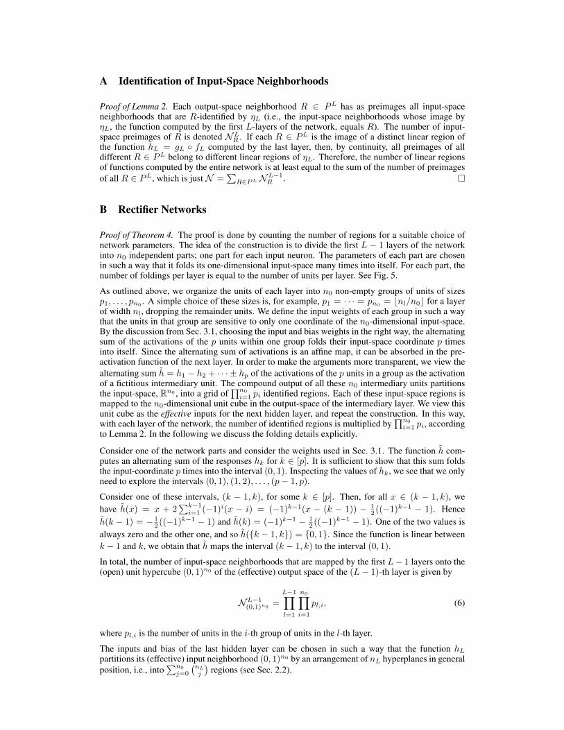
Proof of Theorem 4. The proof is done by counting the number of regions for a suitable choice ofnetwork parameters. The idea of the construction is to divide the first L − 1 layers of the networkinto n0 independent parts; one part for each input neuron. The parameters of each part are chosenin such a way that it folds its one-dimensional input-space many times into itself. For each part, thenumber of foldings per layer is equal to the number of units per layer. See Fig. 5.
As outlined above, we organize the units of each layer into n0 non-empty groups of units of sizesp1, . . . , pn0 . A simple choice of these sizes is, for example, p1 = · · · = pn0 = bnl/n0c for a layerof width nl, dropping the remainder units. We define the input weights of each group in such a waythat the units in that group are sensitive to only one coordinate of the n0-dimensional input-space.By the discussion from Sec. 3.1, choosing the input and bias weights in the right way, the alternatingsum of the activations of the p units within one group folds their input-space coordinate p timesinto itself. Since the alternating sum of activations is an affine map, it can be absorbed in the pre-activation function of the next layer. In order to make the arguments more transparent, we view thealternating sum h = h1 − h2 + · · · ± hp of the activations of the p units in a group as the activationof a fictitious intermediary unit. The compound output of all these n0 intermediary units partitionsthe input-space, Rn0 , into a grid of
∏n0
i=1 pi identified regions. Each of these input-space regions ismapped to the n0-dimensional unit cube in the output-space of the intermediary layer. We view thisunit cube as the effective inputs for the next hidden layer, and repeat the construction. In this way,with each layer of the network, the number of identified regions is multiplied by
∏n0
i=1 pi, accordingto Lemma 2. In the following we discuss the folding details explicitly.
Consider one of the network parts and consider the weights used in Sec. 3.1. The function h com-putes an alternating sum of the responses hk for k ∈ [p]. It is sufficient to show that this sum foldsthe input-coordinate p times into the interval (0, 1). Inspecting the values of hk, we see that we onlyneed to explore the intervals (0, 1), (1, 2), . . . , (p− 1, p).
Consider one of these intervals, (k − 1, k), for some k ∈ [p]. Then, for all x ∈ (k − 1, k), wehave h(x) = x + 2
∑k−1i=1 (−1)i(x − i) = (−1)k−1(x − (k − 1)) − 1
2 ((−1)k−1 − 1). Henceh(k − 1) = − 1
2 ((−1)k−1 − 1) and h(k) = (−1)k−1 − 12 ((−1)k−1 − 1). One of the two values is
always zero and the other one, and so h(k − 1, k) = 0, 1. Since the function is linear betweenk − 1 and k, we obtain that h maps the interval (k − 1, k) to the interval (0, 1).
In total, the number of input-space neighborhoods that are mapped by the first L− 1 layers onto the(open) unit hypercube (0, 1)n0 of the (effective) output space of the (L− 1)-th layer is given by
NL−1(0,1)n0
=
L−1∏l=1
n0∏i=1
pl,i, (6)
where pl,i is the number of units in the i-th group of units in the l-th layer.
The inputs and bias of the last hidden layer can be chosen in such a way that the function hLpartitions its (effective) input neighborhood (0, 1)n0 by an arrangement of nL hyperplanes in generalposition, i.e., into
∑n0
j=0
(nL
j
)regions (see Sec. 2.2).
1st hiddenlayer
intermediatelayer
inputlayer
2nd hiddenlayer
x0
h1(x0)
h1(x0)
h2 h1(x0)
Rn0
Rn1
Rn0
Rn2
0 1
1 1
2
4
2
2
1 1
2
1
11
1 1
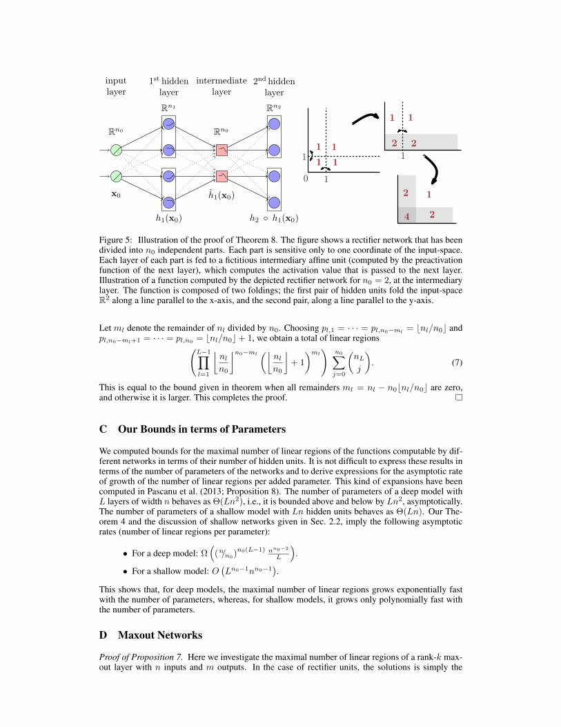
Figure 5: Illustration of the proof of Theorem 8. The figure shows a rectifier network that has beendivided into n0 independent parts. Each part is sensitive only to one coordinate of the input-space.Each layer of each part is fed to a fictitious intermediary affine unit (computed by the preactivationfunction of the next layer), which computes the activation value that is passed to the next layer.Illustration of a function computed by the depicted rectifier network for n0 = 2, at the intermediarylayer. The function is composed of two foldings; the first pair of hidden units fold the input-spaceR2 along a line parallel to the x-axis, and the second pair, along a line parallel to the y-axis.
Let ml denote the remainder of nl divided by n0. Choosing pl,1 = · · · = pl,n0−ml= bnl/n0c and
pl,n0−ml+1 = · · · = pl,n0 = bnl/n0c+ 1, we obtain a total of linear regions(L−1∏l=1
⌊nln0
⌋n0−ml(⌊
nln0
⌋+ 1
)ml)
n0∑j=0
(nLj
). (7)
This is equal to the bound given in theorem when all remainders ml = nl − n0bnl/n0c are zero,and otherwise it is larger. This completes the proof.
C Our Bounds in terms of Parameters
We computed bounds for the maximal number of linear regions of the functions computable by dif-ferent networks in terms of their number of hidden units. It is not difficult to express these results interms of the number of parameters of the networks and to derive expressions for the asymptotic rateof growth of the number of linear regions per added parameter. This kind of expansions have beencomputed in Pascanu et al. (2013; Proposition 8). The number of parameters of a deep model withL layers of width n behaves as Θ(Ln2), i.e., it is bounded above and below by Ln2, asymptotically.The number of parameters of a shallow model with Ln hidden units behaves as Θ(Ln). Our The-orem 4 and the discussion of shallow networks given in Sec. 2.2, imply the following asymptoticrates (number of linear regions per parameter):
• For a deep model: Ω(
(n/n0)n0(L−1) nn0−2
L
).
• For a shallow model: O(Ln0−1nn0−1
).
This shows that, for deep models, the maximal number of linear regions grows exponentially fastwith the number of parameters, whereas, for shallow models, it grows only polynomially fast withthe number of parameters.
D Maxout Networks
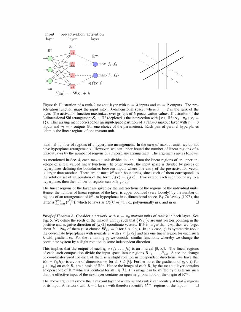
Proof of Proposition 7. Here we investigate the maximal number of linear regions of a rank-k max-out layer with n inputs and m outputs. In the case of rectifier units, the solutions is simply the
f1
f2
f3
f4
pre-activationlayer
activationlayer
inputlayer
x0
f(x0) = Wx0 + b
g(f(x0))
RnRmk
Rm
maxf1, f2
maxf3, f4
Figure 6: Illustration of a rank-2 maxout layer with n = 3 inputs and m = 2 outputs. The pre-activation function maps the input into mk-dimensional space, where k = 2 is the rank of thelayer. The activation function maximizes over groups of k preactivation values. Illustration of the3-dimensional Shi arrangement S3 ⊂ R3 (depicted is the intersection with x ∈ R3 : x1+x2+x3 =1). This arrangement corresponds an input-space partition of a rank-3 maxout layer with n = 3inputs and m = 3 outputs (for one choice of the parameters). Each pair of parallel hyperplanesdelimits the linear regions of one maxout unit.
maximal number of regions of a hyperplane arrangement. In the case of maxout units, we do nothave hyperplane arrangements. However, we can upper bound the number of linear regions of amaxout layer by the number of regions of a hyperplane arrangement. The arguments are as follows.
As mentioned in Sec. 4, each maxout unit divides its input into the linear regions of an upper en-velope of k real valued linear functions. In other words, the input space is divided by pieces ofhyperplanes defining the boundaries between inputs where one entry of the pre-activation vectoris larger than another. There are at most k2 such boundaries, since each of them corresponds tothe solution set of an equation of the form fi(x) = fj(x). If we extend each such boundary to ahyperplane, then the number of regions can only go up.
The linear regions of the layer are given by the intersections of the regions of the individual units.Hence, the number of linear regions of the layer is upper bounded (very loosely) by the number ofregions of an arrangement of k2 ·m hyperplanes in n-dimensional space. By Zaslavsky (1975), thelatter is
∑nj=0
(k2mj
), which behaves as O((k2m)n), i.e., polynomially in k and in m.
Proof of Theorem 8. Consider a network with n = n0 maxout units of rank k in each layer. SeeFig. 5. We define the seeds of the maxout unit qj such that Wi,:i are unit vectors pointing in thepositive and negative direction of bk/2c coordinate vectors. If k is larger than 2n0, then we forgetabout k − 2n0 of them (just choose Wi,: = 0 for i > 2n0). In this case, qj is symmetric aboutthe coordinate hyperplanes with normals ei with i ≤ bk/2c and has one linear region for each suchi, with gradient ei. For the remaining qj we consider similar functions, whereby we change thecoordinate system by a slight rotation in some independent direction.
This implies that the output of each qj (f1, . . . , fk) is an interval [0,∞). The linear regionsof each such composition divide the input space into r regions Rj,1, . . . , Rj,k. Since the changeof coordinates used for each of them is a slight rotation in independent directions, we have thatRi := ∩jRj,i is a cone of dimension n0 for all i ∈ [k]. Furthermore, the gradients of qj fj forj ∈ [n0] on each Ri are a basis of Rn0 . Hence the image of each Ri by the maxout layer containsan open cone of Rn0 which is identical for all i ∈ [k]. This image can be shifted by bias terms suchthat the effective input of the next layer contains an open neighbourhood of the origin of Rn0 .
The above arguments show that a maxout layer of width n0 and rank k can identify at least k regionsof its input. A network with L− 1 layers with therefore identify kL−1 regions of the input.
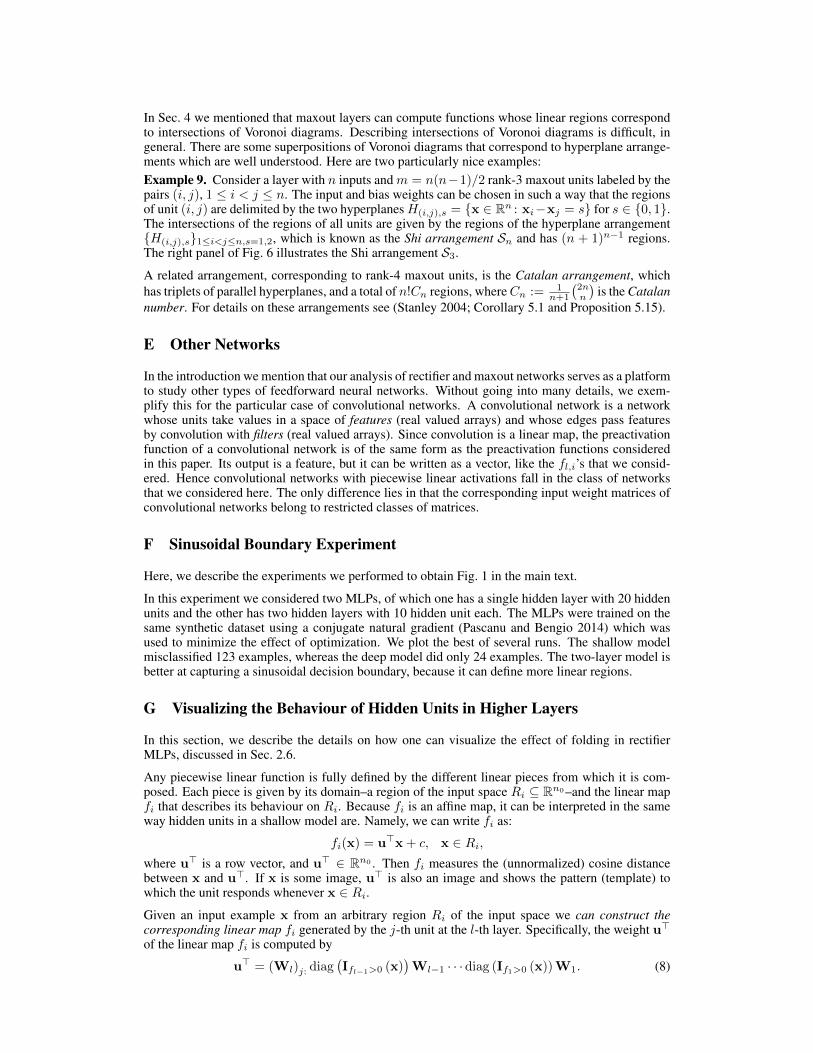
In Sec. 4 we mentioned that maxout layers can compute functions whose linear regions correspondto intersections of Voronoi diagrams. Describing intersections of Voronoi diagrams is difficult, ingeneral. There are some superpositions of Voronoi diagrams that correspond to hyperplane arrange-ments which are well understood. Here are two particularly nice examples:Example 9. Consider a layer with n inputs andm = n(n−1)/2 rank-3 maxout units labeled by thepairs (i, j), 1 ≤ i < j ≤ n. The input and bias weights can be chosen in such a way that the regionsof unit (i, j) are delimited by the two hyperplanesH(i,j),s = x ∈ Rn : xi−xj = s for s ∈ 0, 1.The intersections of the regions of all units are given by the regions of the hyperplane arrangementH(i,j),s1≤i<j≤n,s=1,2, which is known as the Shi arrangement Sn and has (n + 1)n−1 regions.The right panel of Fig. 6 illustrates the Shi arrangement S3.
A related arrangement, corresponding to rank-4 maxout units, is the Catalan arrangement, whichhas triplets of parallel hyperplanes, and a total of n!Cn regions, whereCn := 1
n+1
(2nn
)is the Catalan
number. For details on these arrangements see (Stanley 2004; Corollary 5.1 and Proposition 5.15).
E Other Networks
In the introduction we mention that our analysis of rectifier and maxout networks serves as a platformto study other types of feedforward neural networks. Without going into many details, we exem-plify this for the particular case of convolutional networks. A convolutional network is a networkwhose units take values in a space of features (real valued arrays) and whose edges pass featuresby convolution with filters (real valued arrays). Since convolution is a linear map, the preactivationfunction of a convolutional network is of the same form as the preactivation functions consideredin this paper. Its output is a feature, but it can be written as a vector, like the fl,i’s that we consid-ered. Hence convolutional networks with piecewise linear activations fall in the class of networksthat we considered here. The only difference lies in that the corresponding input weight matrices ofconvolutional networks belong to restricted classes of matrices.
F Sinusoidal Boundary Experiment
Here, we describe the experiments we performed to obtain Fig. 1 in the main text.
In this experiment we considered two MLPs, of which one has a single hidden layer with 20 hiddenunits and the other has two hidden layers with 10 hidden unit each. The MLPs were trained on thesame synthetic dataset using a conjugate natural gradient (Pascanu and Bengio 2014) which wasused to minimize the effect of optimization. We plot the best of several runs. The shallow modelmisclassified 123 examples, whereas the deep model did only 24 examples. The two-layer model isbetter at capturing a sinusoidal decision boundary, because it can define more linear regions.
G Visualizing the Behaviour of Hidden Units in Higher Layers
In this section, we describe the details on how one can visualize the effect of folding in rectifierMLPs, discussed in Sec. 2.6.
Any piecewise linear function is fully defined by the different linear pieces from which it is com-posed. Each piece is given by its domain–a region of the input space Ri ⊆ Rn0–and the linear mapfi that describes its behaviour on Ri. Because fi is an affine map, it can be interpreted in the sameway hidden units in a shallow model are. Namely, we can write fi as:
fi(x) = u>x + c, x ∈ Ri,where u> is a row vector, and u> ∈ Rn0 . Then fi measures the (unnormalized) cosine distancebetween x and u>. If x is some image, u> is also an image and shows the pattern (template) towhich the unit responds whenever x ∈ Ri.Given an input example x from an arbitrary region Ri of the input space we can construct thecorresponding linear map fi generated by the j-th unit at the l-th layer. Specifically, the weight u>of the linear map fi is computed by
u> = (Wl)j: diag(Ifl−1>0 (x)
)Wl−1 · · · diag (If1>0 (x))W1. (8)

A bias of the linear map can be similarly computed.
From Eq. (8), we can see that the linear map of a specific hidden unit fl,j at a layer l is found bykeeping track of which linear piece is used at each layer until the layer l (Ifp>0, p < l – which isthe indicator function). At the end, the j-th row of the weight matrix Wl ((Wl)j:) is multiplied.Although we present a formula specific to the rectifier MLP, it is straightforward to adapt this toany MLP with a piecewise linear activation, such as a convolutional neural network with a maxoutactivation.
From the fact that the linear map computed by Eq. (8) depends on each sample/point x, we needto traverse a set of points (e.g., training samples) to identify different linear responses of a hiddenunit. While this does not give all possible responses, if the set of points is large enough, we can getsufficiently many to provide a better understanding of its behaviour.
We trained a rectifier MLP with three hidden layer on Toronto Faces Dataset (TFD) (Susskind et al.2010). The first two hidden layers have 1000 hidden units each and the last one has 100 units.
We trained the model using stochastic gradient descent. We used, as regularization, an L2 penaltywith a coefficient of 10−3, dropout on the first two hidden layers (with a drop probability of 0.5) andwe enforced the weights to have unit norm column-wise by projecting the weights after each SGDstep. We used a learning rate of 0.1 and the output layer is composed of sigmoid units. The purposeof these regularization schemes, and the sigmoid output layer is to obtain cleaner and sharper filters.The model is trained on fold 1 of the dataset and achieves an error of 20.49% which is reasonablefor this dataset and a non-convolutional model.
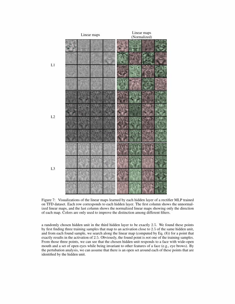
Since each of the first layer hidden units only responds to a single linear region, we directly visualizethe learned weight vectors of the 16 randomly selected units in the first hidden layer. These areshown on the top row of Fig. 7.
On the other hand, for any other hidden layer, we randomly pick 20 units per layer and visualizethe most interesting four units out of them based on the maximal Euclidean distance between thedifferent linear responses of each unit. The linear responses of each unit are computed by clusteringthe responses obtained on the training set (we only consider those responses where the activation waspositive) into four clusters using K-means algorithm. We show the representative linear response ineach of the clusters (see the second and third rows of Fig. 7).
Similarly, we visualize the linear maps learned by each of the output unit. For the output layer, weshow the visualization of all seven units in Fig. 8
By looking at the differences among the distinct linear regions that a hidden unit responds to, wecan investigate the type of invariance the unit learned. In Fig. 9, we show the differences among thefour linear maps learned by the last visualized hidden unit of the third hidden layer (the last columnof the visualized linear maps).
From these visualizations, we can see that a hidden unit learns to be invariant to more abstract andinteresting translations at higher layers. We also see the types of invariance of a hidden unit in ahigher layer clearly.
Zeiler and Fergus (2013) attempt to visualize the behaviour of units in the upper layer, specifically,of a deep convolutional network with rectifiers. This approach is to some extent similar to ourapproach proposed here, except that we do not make any other assumption beside that a hidden unitin a networks uses a piece-wise linear activation function.
The perspective from which the visualization is considered is also different. Zeiler and Fergus(2013) approaches the problem of visualization from the perspective of (approximately) invertingthe feedforward computation of the neural network, whereas our approach is derived by identifyinga set of linear maps per hidden unit.
This difference leads to a number of minor differences in the actual implementation. For instance,Zeiler and Fergus (2013) approximates the inverse of a rectifier by simply using another rectifier. Onthe other hand, we do not need to approximate the inverse of the rectifier. Rather, we try to identifyregions in the input space that maps to the same activation.
In our approach, it is possible to visualize an actual point in the input space that maps to the sameactivation of a hidden unit. In Fig. 10, we show three distinct points in the input space that activates
L1 Linear maps Linear maps(Normalized)
L1
L2
L3
Figure 7: Visualizations of the linear maps learned by each hidden layer of a rectifier MLP trainedon TFD dataset. Each row corresponds to each hidden layer. The first column shows the unnormal-ized linear maps, and the last column shows the normalized linear maps showing only the directionof each map. Colors are only used to improve the distinction among different filters.
a randomly chosen hidden unit in the third hidden layer to be exactly 2.5. We found these pointsby first finding three training samples that map to an activation close to 2.5 of the same hidden unit,and from each found sample, we search along the linear map (computed by Eq. (8)) for a point thatexactly results in the activation of 2.5. Obviously, the found point is not one of the training samples.From those three points, we can see that the chosen hidden unit responds to a face with wide-openmouth and a set of open eyes while being invariant to other features of a face (e.g., eye brows). Bythe pertubation analysis, we can assume that there is an open set around each of these points that areidentified by the hidden unit.
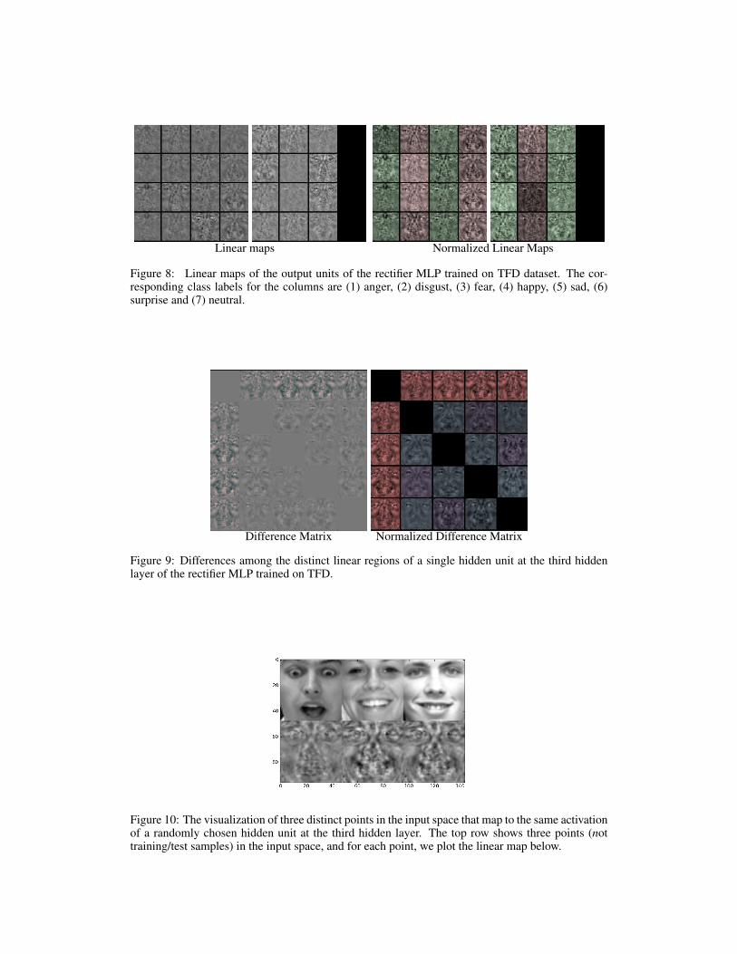
Linear maps Normalized Linear Maps
Figure 8: Linear maps of the output units of the rectifier MLP trained on TFD dataset. The cor-responding class labels for the columns are (1) anger, (2) disgust, (3) fear, (4) happy, (5) sad, (6)surprise and (7) neutral.
Difference Matrix Normalized Difference Matrix
Figure 9: Differences among the distinct linear regions of a single hidden unit at the third hiddenlayer of the rectifier MLP trained on TFD.
Figure 10: The visualization of three distinct points in the input space that map to the same activationof a randomly chosen hidden unit at the third hidden layer. The top row shows three points (nottraining/test samples) in the input space, and for each point, we plot the linear map below.