Embed Size (px)
Citation preview
arX
iv:1
711.
0054
7v2
[co
nd-m
at.s
tat-
mec
h] 9
Nov
201
7
Time Evolution and Thermodynamics for the
Nonequilibrium System in Phase-Space
Chen-Huan Wu ∗
College of Physics and Electronic Engineering, Northwest Normal University, Lanzhou 730070, China
November 10, 2017
The integrable system is constrained strictly by the conservation law during thetime evolution, and the nearly integrable system or nonintegrable system is also con-strained by the conserved parameters (like the constants of motion) with correspond-ing generalized Gibbs ensemble (GGE) which is indubitability a powerful tool in theprediction of thr relaxation dynamics. For stochastic evolution dynamic with consid-erable noise, the obviously quantum or thermal correlations which don’t exhibit thethermal behavior, (like the density of kinks or transverse magnetization correlators),display a asymptotic nonthermalization, and in fact it’s a asymptotic quasisteadystate with a infinte temperature, therefore the required distance to the nonthermalsteady state is in a infinite time average. In this paper, we unambiguously investi-gate the relaxation of a nonequilibrium system in a canonical ensemble for integrablesystem or nonintegrable system, and the temporal behavior of many-body quantumsystem and the macroscopic system, as well as the corresponding linear-coupling be-tween harmonic oscillators. Matrix-method in entropy ensemble is also utilized todiscuss the boundary and the important diagonalization, the approximation by theperturbation theory is also obtained.
1 Introduction
The investigation of evolution of nonequilibrium system is important to the particle physicsor condensed matter physics and even the cosmology (like the entropy of Bekenstein-Hawkingblack hole1)), especially in the many-body theroy prediction which by, e.g., the trapped ul-tracold atomic gases which have weak energy interaction with the environment and thereforeallow the observation of unitary time evolution2). For nonequilibrium system, the usualy formof glass can be blocked by the pinning field3) and prodece a galss transition like the process ofergodic to non-ergodic, In replica theory, since the homogeneous liquid given by replica sym-metry have a inhibitory effect for entropy production, whereas the replica symmetry brokenresult in the increase of overlap of replicas. With the increse of degree of overlap which canbe realized by enlarge the system size, the number of metastable states (or the hidden one) isgrows exponentially, and furthermore, the entropy is grows logarithmic.
We already know that the observable chaotic classical system require the processing resourcewhich increase exponentially with time and Kolmogorov entropy h4) due to it’s exponential sen-sitivity in initial state5), while the integrable one, which is solvable by the Bethe ansatz6), isincrese polynomially. The time evolution of quantum entangled state may cause decoherenceeffect which is widely found in condensate system and it take a important role in quantuminformation processing, quantum computation and metrology, quantum teleporation, quantum
1
key agreement7,8), and even the decoherence in neural network9). The entanglement is mostlypreduced by the dynamical evolution with nonlinear interaction10) and the non-destructive mea-surement. like the Dzyaloshinskii-Moriya interaction11,12), and in extreme case, e.g., through theaxion field13,14). Usually the quantum entanglement is studied by the two-qubit or qutrit11,15)
system, in some case the tripartite system12,16) or even more one is consider. In nonequilibriumand nonstationary open system, the coarse graining which connecting numerous subsystems’degrees of freedom make more possible to realize this process17), and the thermal entropy is agood measurement for the effect of coarse graining. The quantum spaces’ dimension increasesexponentially with particle number due to the tensor-productor5), similarly, the number ofmetastable which as the subsystems of the spin glasses system is increase expnonentially withsize in high temperature18), phase transition and critical fluctuation occur when it from onekind of subsystem into another and the broken and restoration of symmetry is also affect theproperties of materials19), like the dielectric constant, etc.
In solid-state quantum system, the spin is the best candidate among various microscopicatom intrinsic degrees of freedom in thermal entanglement which has higher stability comparedto other entanglements due to the spins’ relatively long decoherence time20) and it’s in closeconnection with the local free erengy. The long coherence time in many-body systems is usefulto detecting the unitary dynamics, e.g., the Hubbard-typr model, and it’s important to thecoherent nonequilibrium dynamics for the multiple phases transition. Since the models thatcan be mapped to a spinless free fermions through Wigner-Jordan transformation and show ain-phase fermion liquid state21), have show a stationary behavior in such a equilibrium inter-grability model which consider as a powerful tool to obtain the exactly solution of model22). Anumberical method as time-dependent density matrix renormalization group (t-DMRG) haveshow that the matrix produce operator D(t) is simulation-inefficently for nonintegrable modelwhich is similar to the tensor-productor, but it’s efficent for integrable and local disordedcase23). Except that, the method of matrix produce wave function is also a good tool to dealwith this time-evolving one-dimension quantum system24). The time evolution on free fermionsor bosons, when the time scale to infinity the thermal average of z-component spin Sz is zeroand the spin states is half-filled21), in this case the interaction between particles is strongest dueto the zero-polarization23), and the entanglement entropy is also increase and becomes moreextensive25). The first implementation of using the density matrices in prediction of many-bodysystem (equilibrium or nonequilibrium) is the Ref.26). It discuss the situation similar to thequantum irreversible process in a energy- and information-lossy system.
A fact that the many-body quantum system will tend to equilibrium has been verifiedby many rencently experiments, like the trapped ultracold atoms in optical lattices or theinteractions with optical resonance. Whereas for the nonequilibrium system, the relaxtion andthermal entanglement and the stochastic force also attract a lot of attention27,28). Furthermore,the system may relax to analogue of thermal state if the inital state is ground state27). Themethod of fluctuation-dissipation relation (FDR) and quantum state diffusion (QSD) is utilizedfor the evolution to steady states in integrable system whose final states are constrainted by theconserved law (indeed, it’s the scattering process of particles which constranted by conservedlaw) and with a finite speed of algebraically relaxation and information transfer under thethermodynamic limit (the large-N limit). Note that the speed here will not bounded by thespeed of light like the relativistic quauntum theory, but bounded by a well known Lieb-Robinsongroup velocity29). The integrable system of quantum Newton’s cradle with groundbreaking isa example30). The classical system also have found the same reslut, like the Fermi-Pasta-Ulam (FPU) theorem31) and Kolmogorov-Arnold-Moser (KAM) theorem32). While for somenonintegrable system, the constant of motion can be expressed by second quantized operator33)
(see below).The collection variables are applied to investigate the evolution in studied system, except
2

this, we also applied the method of density matrix and complex tensor grid to make this paperself-contained. For local observable system the stationary and linear value may exist (likethermal state), but for integrable system whose time evolution found no thermalization and itmay tends to a distribution of GGE with a important fundamental hypothesis for statisticalensemble that has maximized entropy which is constrained by local conservation law34), (e.g.,the conservation quantity of momentum occupation number), hence restrict the ergodicity andcan’t reach the thermal state. For a framework of macroscopic system in finite dimension isimportant to introduce the quantum field theory for both the equibrum and nonequibrum statein open system17) to investigate its time-dependent nature and coupling (or interaction) in localand nonlocal case as well as the dynamical fluctuation in short distance. It’s also necessary toconsider a quantum field when the Hilbert space is too large to implement a well numbericalsimulation35). While the importance of entangled states for quantum computation is wellunderstand, to reduce the confusion from decoherence, there is a topology way that storingthe quantum information non-localized36) or through the non-Abelian braiding statistics whichsupport the Majorana fermions37,38) by Majorana modes in finite wire39), and it can bettersolve the problem of infinety dilution of the stored information in local area27).
Since for nearly integrable system, the behavior of relaxation is under the crossover ef-fect of prethermalization and thermalization, which is associate with the thermal correlationand the speed of information transfer, and the prethermalized state can be well described bythe GGE40), i.e., may be view as a integrable system. Like the Ref.41) which also using themethod of t-DMRG and show the nonthermalization in soft-bosons model, have perform theoff-diagonal correlation in the two-dimension square model, and the relaxation with some fluc-tuation is presented in short time evolution. The suppressed thermalization can be freed byenough perturbation to break the integrability. This crossover effect affect both the noninte-grable system and open system. Through the study of this paper, we know that the recurrencewill appear for large time evolution. In the configuration which considered in this paper, partof mixed system which is of interest is coupling with the environment (not isolated), and hencethe degrees of freedom of environment system (i.e., the counterpart of the target one) can betraced out in the canonical ensemble32), i.e., tracing over the variables outside the target re-gion. This provide the support on the matrix method in Sect.10. A large number of degrees offreedom is also a important precondition to implement global relaxation with the thermody-namic limit42). For nonlocal operators in equilibrium state, the dynamical parameters displaya effective asymptotic thermal behavior (follow the Gibbs disturbution)43) during equilibriumtime evolution with determined temperature and decay with a asymptotic exponent law, whilethe model what we focus on is towards the asymptotic quasisteady state with a infinte tem-perature, which decay with a asymptotic power law6) acted by a diffusion term (see Sect.11).The prethermalization will shares the same properties of nonthermal steady state due to thedynamical parameters, which makes the model after quench close to the integrable points (orsuperintegrable point). But in fact, for integrable quenches, the stationary behavior for boththe local and nonlocal observables can be well described by the corresponding GGE, and theparticles scattering which constranted by conserved law is purely diagonal44,45).
This paper is organized as follows. We introduce the model of two-coupled subsystemin Sect.2, and the bare coupling is further discussed in Appendix.A. The evolutions in non-dissipation system is discussed in Sect.3, and the quenching for many-body system is diacussedin Sect.4. A system-environment partition is mentioned in these two section. In Sect.5, wediscuss the dissipation for nonlocal model. In Sect.6, the time evolution and thermal entangle-ment of Heisenberg XXZ model is investigated. In Sect.7, the correlation and transfer speedof information in quantum system is discuss where we take the one-dimension chain modelas the explicit example. The relations between thermal behavior and the integrability is alsodiscussed in this Section. We discuss the nonequilibrium dynamics with strong and weak in-
3

teraction in Hubbard model in Sect.8. In this section, we investigate the phase transition ofnonintegrable Hubbard model, and the relaxation of double occupation and the kinetic energy.We also use the method of nonequilibrium dynamical mean-field theory (DMFT) to detect theevolution by mapping the lattice model to the self-consistent single-site problem which can besolved numerically. In Sect.9, we discuss the relaxation to a Gaussian state. In Sect.10, weresort to the matrix method, and the propertice of the boundary and the transfer speed arealso discussed. In Sect.11, we discuss the relaxation of nonequilibrium system with stochasticdynamical variables in a free energy surface, the quantum dissipation in the damp-out pro-cess is also discussed. The diagonal contribution to symplectic spectrum of covariance matrixis further detected in Appendix.B. The bulk-edge-coupling type materials which is related tothe spectrum gap is presented in Sect.10 and Appendix.C, and the perturbation therory anddiagonalized Hamiltonian is also discussed in Appendix.C.
2 Model Introduction and the Coupling in Feild Theory
We begin with the perturbation theory with space-time dimension, which is important toconsider in the strong coupling case32), weak-perturbation limit of nonintegrable system, andeven the breaking of ergodicity3). In dimension of (d+1) in sapce-time, since the particles obtainmass from the broken of non-Abelian gauged symmetry, the couping constant g is dimension-dependent, except the bare couping gb which vanish in d + 1 = 4 limit46). the broken transla-tional symmetry also make the spin liquid state rapidly solidified and turn into the crystallinesturcture19,47). Then we define two d-dimension system ψi and ψj with potential φi and φj,respectively. In weak couping condition which suitable for the perturbative calculation19), thereis exist a spin density wave (SDW) which in a Fourier expression is ψi = L−d
∑
i e−iqriφ(x− ri),
and ψj is as the same form. Although the L here is constrained by the model dimension d,but L itself could be dimensionless and with dimensionless length scale and time scale (seeRef.48)). The φ here describe the fluctuation as a function in arbitrary dimension, and it’salso useful for quantum fluctuation or even the vacuum fluctuation. The dimension of φ mayeven up to ten according to D-branes of string theory49). In the space dimension of d = 3, thekitaev model despict a triangular parameter space with different degrees of coupling in threedirection x y and z, and the small triangular area which connecting the three midpoints ofthree side is gapless phase region50). In this model, I set coupling in these three direction ina range of 0 to n, for which the top value n is n = 2d/2N in SO(d)× SU(N) system51). So acontinuous phase transition with weak coupling pertubative RG under the time evolution canbe expressed by S =
∫
ddxL which is a exponent appear in the imaginary-time path integral
Z =∫
Dψ†iDψiDψ
†jDψje
−S 52).
The nonrelativistic Lagrange L is46,49)
L =
∫ τ
τ ′dτ [(iψ†
i ∂τψi +1
2µψ†i∇ψi − µψ†
iψi) + (iψ†j∂tψj +
1
2µψ†j∇ψj − ηψ†
jψj)], (1)
where τ and τ ′ is initial and final time, ∇ is the Laplace operator, and η is the chemicalpotential. This time evolution Lagrange ignore the interactions, e.g., the inpurity induced longrange order49,53). Since the half integer spin correponding to the gappless area which mentionedabove, the fermion system in this area can be written as H =
∑
a=x,y,z Ja∑
〈i,j〉a ψiψai ψjψ
aj ,
(a = x, y, z), with ψiψai = si/i and ψjψ
aj = sj/i, then we have H = −
∑
a=x,y,z Ja∑
〈i,j〉a sisj. In
Eq.(1) we take the imaginary time approach which the quantum Monte Carlo (QMC) methodis utilized54), the differential symbol ∂τ has the below relation according to the definition ofBernoulli number55)
4
n∂τ (τ 1−z
1− z) =
τ 1−z
1− z
∞∑
n=0
Bn(−∂τ )nn!
, (2)
and the differential symbol for mass is as the same form
n∂µ(µ1−z
1− z) =
µ1−z
1− z
∞∑
n=0
Bn(−∂µ)nn!
. (3)
The Gardner transition which the critical dimension dc = 3 is a important object in studyof properties of amorphous solids56). In (3+1) space-time dimension using the renormalizedcoupling, since the bare coupling is absent in the dimension d+1 = 4, the resulting dimensionlessbare action with unbroken Quantum electrodynamics (QED) symmetry is
S =
∫
dx
1
2
n∑
x,y=0
[(∂µφxy)2 + rφ2
xy]−1
3!(gbi
n∑
x,y=0
φ3xy + gbj
n∑
x,y,z=0
φxyφxzφyz)
, (4)
and the action of Landau-Ginzburg-Wilson (LGW) Hamiltonian with N-component O(N) sym-metry and noncollinear order is57)
S =
∫
ddx
∫ τ ′
τ
dτ
1
2
n∑
x,y=0
[(∂µφxy)2 + rφ2
xy]
+1
4![gi(
n∑
x,y=0
φ2xy)
2 + gj
n∑
x,y,z=0
[(φxyφz)2 − φ2xyφ
2z]]
(5)
The summation index xyz range from zero to n − 1 corresponding to the parameter spacesetted above, and the average term
∑nx,y,z=0 [(φxyφz)2 − φ2
xyφ2z] exhibit the correlation between
these two fluctuation functions. Using the method of time dependent density matrix RG whichhave been proved valid for particles at a fixed evolution time23), this fermion system shown asTijδij = Trσiσj where Tij is the interaction tensor, the σi and σj are the matrices of ψi and
ψj respectively and δij = cic†j. This expression is indeed take the diagonal part of Tij . Ref.46)
put forward a valuable view that connecting the bare coupling to the renormalized coupling bya infinte cutoff, and then the mass-independent bare coupling can be shown as46)
gb = µ3−d
g + δ11g3
3− d
+ δ21g5
3− d+ δ22
g5
(3− d)2
+ δ31g7
3− d+ δ32
g7
(3− d)2+ δ33
g7
(3− d)3+O(g9)
,
(6)
which is satisfactory consistent with the series expansion of β function given in Ref.58)
β(g) = −β0g3
16π2− β1
g5
(16π2)2− β2
g7
(16π2)3− O(g9). (7)
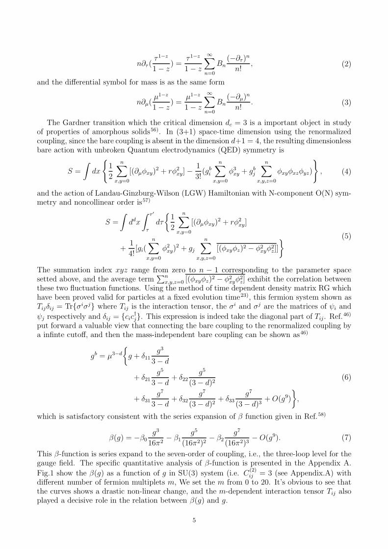
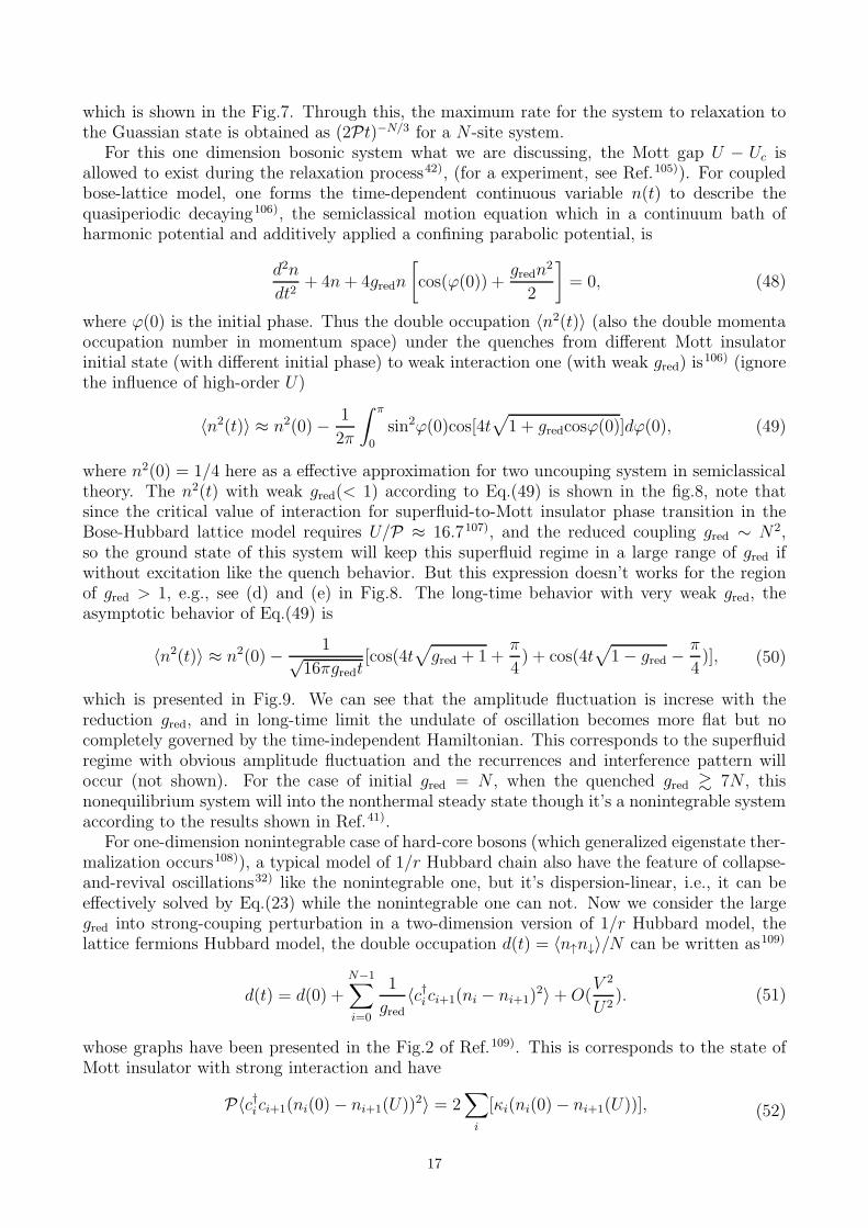
This β-function is series expand to the seven-order of coupling, i.e., the three-loop level for thegauge field. The specific quantitative analysis of β-function is presented in the Appendix A.
Fig.1 show the β(g) as a function of g in SU(3) system (i.e. C(2)ij = 3 (see Appendix.A) with
different number of fermion multiplets m, We set the m from 0 to 20. It’s obvious to see thatthe curves shows a drastic non-linear change, and the m-dependent interaction tensor Tij alsoplayed a decisive role in the relation between β(g) and g.
5
3 Evolution Behavior in Non-Dissipation System
Since the long time scales exist in the metastable states which the quantity grows exponen-tially with system size19), e.g., the single positive charge state in p-type material59) or the p-spinmodel60). the imaginary-time path integral can be expressed by the trace of time evolution op-erator Z = Tr(e−βH) with the evolution propagator U = e−βH = Tr(σi
1σi2 ···σi
nσj1σ
j2 ···σj
n), whereβ is inverse temperature 1/T which we use the unit of Boltzmann constant k = 1 Note that thespin pauli matrix here is contain all the component in finite dimension of Hilbert space and Hij
is the nearest neighbor Hamiltonian and can be decomposed using the Trotter-Suzuki methodwhich mapping the one dimension quantum system into two dimension61) and the path integralis becomes Z = Tr(Πi,je
−βHij ), In this way, the long range interaction can be treated locallyas a nearest-neighbor pair in this spin isotropic system through a single two-qubit exchangegate Ui,i+1 = e−Hi,i+1δτ due to the iterative nature and acting on two adjacent site with singletime step δτ evolution, it is also meets with the realignment criterion15), that is, the local fieldeffect. Then we have
e−βHi,i+1 =∏
i
Ui,i+1. (8)
Except the Andenson localization, the local length may strongly increase obey the logarith-mic law62). The Hamiltonian here was divided by the partition function Z through the temper-ature interval or the external magnetic field h51). By investigate the asymptotic behavior of Z,when β → ∞, i.e., the temperature decrease with the imagnary time evolution, the Z → 0, andthe system tends to the ground state which is |ψ(0)〉 = |ψi
1〉⊗|ψi2〉···⊗|ψi
n〉⊗|ψj1〉⊗|ψj
2〉···⊗|ψjn〉,
and denote the εn′ is the energy of the n′th level (n′ < n) in this system above the ground
state, εn′ = En′ − En′−1. Then the pauli operator σi/jn′ within the evolution propagator U is
σi/jn′ = σ0⊗n′ ⊗ σ
i/jn′ × σ0⊗(n−n′) 5) Before that happen, the entanglement between paiticles which
depending on time rapidly reaches the maximum value, which make the method of time de-pendent density matrix RG invalid due to the too large growth speed of entanglement entropy.The evolution by the evolution propagator U is
|ψ(β)〉 = U |ψ(0)〉, (9)
and specifically, in the form with imaginary-time analogue eτH(τ) it has24,63)
|ψ(τ)〉 = eτH(τ)|ψ(0)〉|| eτH(τ)|ψ(0)〉 || , (10)
where we define the imaginary-time as τ = t + i0+, while for the evolution Hamiltonian isH(τ) = eαHHe−αH where α = β + i0+. Since ∂βψ(β) = Hψ(β), we have β ∝ (∂τ )
n, which isalso shown in the Eq.(2). For thermal average of a imaginary-time-dependent quantity F , itsexpectation value which describe the ensemble average can be written as
〈Fτ〉 =〈ψ(τ)|F|ψ(τ〉)〈ψ(τ)|ψ(τ〉) , (11)
where 〈ψ(τ)|ψ(τ〉) is the partition function here, and the accurate value of 〈ψ(τ)|ψ(τ〉) and〈ψ(τ)|F|ψ(τ〉) can be determined by the method of tensor RG. The cumulative effect is effi-ciently in this averaging process27) and often do a cumulant expansion at the expectation valuefor simplified result whose truncation depends on the detail of dissipation64). Through this, aworld-line tensor grid RG can be formed by taking coordinate as the horizontal axis, and thetime (or temperature) as vertical axis, i.e., form a tensor network. The tensor network separatedby the inverse temperature β have the spacing ζ = β/M whereM is the total number of lattices
6
in the network (also called the Trotte number61)). Such a method which utilize the evolutionof time and phase also called Trotterization65). Through the theory of t-DMRG, the F can betreated as a matrix product operator which depends on the time-evolution, Fτ = U(τ)FU †(τ),here Fτ and F base on different basis. With the nonequilibrium time evolution, the integrablesystem which has the important feature of localization will relax to the stationary state afterquantum quenches, i.e., the suddenly change of interaction strengh27), and the density matri-ces which constraint by the expectation value will leads to a maximum entropy ensemble25).Usually we model the integrable (superintegrable) model by choosing the special initial state,typically, like the XY spin model, and it can be affected deeply by the constants of motion inthe integrable (superintegrable) points like reach the nonthermal steady state and so on. Thedensity matrices here is denpends exponentially on conserved quantity and the Hamiltonianswhich related to the initial state. For the matrix-product operators which describe the quantumstates, the minimal rank D is requied to the maximal one of the the reduced density matrixof bipartition system5) (i.e., bipartition of the target one and its enviroment) and it neededto truncated by the method of singular values decomposing to keep the size of D polynomialincrease which is local and time-computable, and we keep only the largest singular values afterthe truncation, i.e., only keep the basis states66). In fact, for dissipation system, the linear ornonlinear dissipation coupling accompanied by the phase noise67) (like the Wiener noise (seeSect.11)) as well as the white noise or colored one68) also have inhibition on the exponentialincrease.
In Schrodinger picture, the observables of thermal states are achieved by carry the integrablesystem into the nonintegrable one (by perturbations) and in the mean time the energy-levelspacing disturbution is evolves from the Poisson distribution with diagonal matrices to theGaussian one (i.e., the wigner-Dyson type one) with level repulsion and random symmetricmatrices69) (there are also symmetrically ordered operators in quantum dynamics by Wignerrepresentation48)). It’s possible to back to the Possion distribution by applying a series of singlegate which prevent the exponential increase of rank D but introduces the norm error23)
η =
n−1∑
i=0
(1−D−1∑
j=0
λ2j(Ui)), (12)
where Ui is a single gate and λj(Ui) is the decreasing ordered singular values after removingthe maximum one, and the maximum entropy is accessible through the local relaxation and thesame as the entanglement. Although for nonintegrable system the growth of D is founded to beexponential, there exist methods like the diagonalization which keep the size of matrix alwaysproportional to the time (or the system size), like Bogoliubov rotation (see Appendix.C). Theprocedure of eliminating the small singular values result in a low-rank matrix, and this is alsoto keep the local free energy
Efree = − 1
βln(
∑
i
λ2i ) (13)
smallest (λi is the singular values), and also to enhance the equilibrium characteristics whichtreated as a thermodynamics anomaly in glass system70). This equation also explicitly showthe measurement of erengies in units of (inverse) temperature. To solve the problem of densitymatrix in the t-DMRG, one introduce a way to solve the rank minimization problem whichmake this method valid even for the low rank matrices (see Ref.71)), and it’s help to reducingthe error and keep computational cost low at the same time. On the other hand, that alsoprovide the convenience that make the matrix nondecreasing and so that the maximum rankis always appear in the final step of the algorithm.
Since we have implement the system-environment partition, in a full quantum dynamics, wecan yield a well approximation in the weak-couping regime by the low-order truncation, e.g.,
7

the wigner truncation approximation which truncate in the power of one-order48). In such aphase space, the coupled two subsystem have the relation
∑
ki,kj(−ki!/Aki)gki(−kj !/Akj)gkj =
∑
k(−k!/Ak)g2k 19), where k is the number of powers of truncation in phase space (e.g., k = 1when truncate in the first-order) and A is the angles which dominate the series expansion ofthe dimensionless coupling g (see Sect.2).
From the discussion on this Setction, we can see that the imaginary-time propagation has thesimilar behavior with the real-time one, it will provide us another way to detect the decayingprogress including the die out of excitations, and it’s available for similar real-time setups54),or application to the nonequilibrium problem with stochastic series expansion in integrablesystem without the constraint of local conservation law. Therefore it’s more feasible to detectthe asymptotics phenomenon in time evolution, expecially for the low-order perturbation theroywith extended potential.
4 Quenching in Many-Body Local System
For integrable open system, we imagine the bipartion of the Hilbert space and into thetwo formulated finite-dimension linear space (two associated configuration) Vi and Vj whichassumed have same spectrum and their reduced density matrices are
Ji =
R∑
R=1
λR|ψiR〉〈ψi
R|, (14)
Jj =R∑
R=1
λR|ψjR〉〈ψj
R|, (15)
where λR is the Schmidt coefficients (the decresing singular values). The bipartite state |ψ〉 ∈Cdi ⊗Cdj which realized through the Schmidt decomposition via singular value decomposition,and the Schmidt rank is min[di, dj]
72). For inseparable case, the reduced density matrix J ′
i (ifit’s pure state density matrix with feature of unitarily invariant) can be obtained by tracingover the the pure state in its extended subsystem (i.e., Cdj ), and the product space which formby two subsystem is Vi ⊗ Vj . This bipartition can be used in most of the quantum many-bodymodel, like the Ising transverse field model, XXZ model, and kitaev model, ect.
Integrability is usually relies on the localization, especially the superintegrable one (like theXY spin model) which are fully relies on the localization34). For a concrete example, we considera XY spin two-chain model without the magnetic field, which the bulk Hamiltonian is73)
Hi,i+1 =N−1∑
i=0
1
2(σx
i σxi+1 + σy
i σyi+1) · exp[
J
4
N−1∑
j=0
(σ2xi+Θ(j−i) + σ2y
i+Θ(j−i))], (16)
where J is the coupling, i, j stands for the different chains, and Θ(j− i) is a step function. Thecorrelation in such a system is18)
〈si, sj〉 =1
N − 1
∑
ij
sisj =1
2qij(N − 1), (17)
where qij is the overlap between these two spin configuration. The local quantum integrabilityin the bounded bulk model can be deriving by the explicit form of the quantum R-matrix aswell as the boundary transfer matrices, e.g, see Ref.34,73,74).
For quench behavior due to the perturbation from local operators, which for the out-of-equilibrium protocol is striking, the amplitude from initial state to instantaneous n state is75)
8

An(t) = −∫ tf
ti
dt〈n|∂t|0〉exp[i(ϕn(t)− ϕ0(t))] (0 ≤ i ≤ n), (18)
where ϕ(t) is the dynamics phase. Such a amplitude is also the eightvalue of density matrices inentropy ensemble with the specific heat
∑
n[En −E0|An(t)|2. The sum of square of amplitudesis the excitation probability Pex =
∑
n |An(t)|2 for electrons, particles, or holes, i.e., quenchedaway from initial (ground state) to new state. Here we suppose the quench is very fast thatthe initial state ψ0 and the quenched state ψn are amlost exist at the same time ti. Then usingthe evolution propagator U(t), we obtain the amplitude76)
〈n|U(t)|0〉 = −i〈n|∫ tf
ti
dtH(t)|0〉
= −i〈i|Hint|0〉∫ tf
ti
dt′exp[i(En − E0)t′]
= −〈i|Hint|0〉exp[i(En − E0)t]− 1
En − E0
,
(19)
where E0 is the energy in the initial state ψ0 Through the fermi golden rule, where Hint is theinteraction Hamiltonian with scattering amplitude Ai, which is
Hint =U(t)(En − E0)
√
2− 2cos[(En − E0)t]. (20)
For further detect the perturbation from local operators, we present in Fig.2 (a) the energydifference between the excited state and initial one with different staggered magnetic field hsin different dimension D of a quantum lattice model, and (b) the excitation probability as afunction of the temperature, it’s clearly that the probability distribution obey a Gaussian form.Since the quantum noise comes from the random initial state, we define a Gaussian in the initialstate white noise which have a zero mean and therefore the initial probability distribution isGaussian. Then the probability distribution in the process of relaxation is77)
P =∑
m,n
δ[∆E − (Em(t′)− En(ti))]|〈ψm(t
′)|U(t)|ψn(ti)〉|2|〈ψn(ti)|ψ0(ti)〉|, (21)
where δ is the amplitude of the Gaussian (see Sect.11) and ∆E is the energy-difference betweenthe initial and final state of relaxation. In phase space, such a relaxation can be expressed bythe density matrix
J (t) =∑
k,k+q
exp[−φ(k)t]J (0) =∑
k,k+q
exp[−(Ek+q − Ek)t]J (0), (22)
where k and k+ q are two spectral parameters. For slow quench which the time scale toinfinity, the non-diagonal contribution to J (t) (i.e., the part of q 6= 0) is vanish due to the fastoscillation of Fourier kernel exp[−(Ek+q − Ek)t].
In fact, the non-diagonal contribution to the mean-field-representation (or the second mo-
ments of the disturbution of momentum27)) 〈cic†i+1〉 =∫
dnkf(k)cos(ϕ(k)t) is asymptotically to
a fixed value with the time evolution41). When a external perturbing field is considered in thefree energy landscape, a perturbing term should be added to the local free energy, and since theperturbation is bad for the conservation of energy, the quantum system under the influence ofnoise variables will not completely isolated even for the closed quantum system. The couplingbetween this perturbing field and the Hamiltonian is beneficial to enhance the system ergodicity
9

by increase the coupling of metastates. For closed system which have total energy conservation,the ergodicity for observables under the long-time limit can be large enough to expect the timeaverage to the thermal average33), but there are restriction on the observables like the boundof the von Neumann entropy, and hence prevent it closing the thermal state. (Note that herethe correlation between each distinguishable particle and the environment is still localized.)The entropy of pinning field is increase with the overlap in a metastate, can associate withthe hidden glass states, and it’s confirmed equal to the mean field potential of glass system78).Both the entropy Shidden (not the diagonal one) and its free energy as well as the non-diagonalcontribution vanish in the final of the process of relaxation to steady equilibrium state, e.g.,the commensurate superfluid state.
Since for the integrable system, most solvable Hamiltonian can be mapped to the effectivenoninteracting Hamiltonian32)
Heff =N−1∑
i
ǫiPi (23)
with the eigenenergy ǫi and conserved quantity Pi, and the maximum entropy ensemble afterquench with local conserve-law can be written using the density matrix as
Jquenched =1
Zexp(−
∑
i
PiYi), (24)
where the conserved observable quantity Pi has the form Pi = a†iai where ai is the annihilationoperator of bosons or fermions and has commute relation [H,Pi] = [Pi, P
′i ] = 0, the Yi is a initial
state-dependent quantity. The partition function Z = Tr[(exp(−∑
i PiYi))]. This is in fact onlya local steady state but not canonical steady states for the full system25). For integrable systembegin with the maximal entropy in GGE, the Yi here can be replaced by a Lagrange multiplierset λi32,34,79,80), (which is81) λi = ln[(1 − 〈ψ(0)|Pi|ψ(0)〉)/〈ψ(0)|Pi|ψ(0)〉] and constrainedby 〈n〉GGE = 〈ψ(0)|c†c|ψ(0)〉 = Tr(ρn) where n is the conserved number of particles). Forintegrable systems which are exact solvable (i.e., all the eigenvalues and eigenfunctions can beobtained), since the ǫi is linear eigenenergy, for a simplest conserved quantity, the number ofparticles ni, the number eigenstate can be treated as the energy eigenstate E =
∑
i ǫini whichon the eightbasis of ni48).
Within the scheme of adiabatic perturbatic 〈k · p〉 theory, the asymptotic behavior be ma-nipulated by the velocity and acceleration of tuning parameter in quench dynamic75). Thetuning-dependent Hamiltonian ψ(λ(t)) (λ(t) is the time-dependent tuning parameter) can alsotake effect in the adiabatic excitation of system in ground state which is similar to ψ(t), andrecover due to the asymptotic effect of time evolution54). The asymptotic freedom of systemwill preserved until the number of fermion species is too large58), so this asymptotic state withthe scaling theory is depend only on the configuration, e.g., the fluctuation of system18,54,82),and scales show a collection of the effects from fluctuation and tend to Gibbs value when themomentum vector q → 082). One of the reflection is the equilibrium Gibbs free energy asbelow3) (without restrictions)
EGibbs = − 1
βln
∫
dte−βH(t), (25)
and since the Hamiltonian here is often the potential field-characterized, the free energy alsotreated as a potential function with determined weigh (probability distribution).
10
5 Dissipation in Nonlocal Model
For nonlocal model, there is a large different compare to the local one. The nonequilibriumlong-range force is also usually unobservable in localiaed interaction models83). Consider theYang-Mills theory, the action of field can be expressed as
S =1
4
∫
ddx
∫ t′
t
dtF µνi F i
µν , (26)
where F µνi is the field strength tensor (see Appendix.A), F µν
i = ∂µAiν − ∂νA
νµ − gCiabA
aµA
bν84),
where Aaµ and Ab
ν are the vector potential of the field and here Ciab is for intruduce a SU(3)
structure factor which is Ciab = γiabF aF b, where γiab is the SU(3) structure constant and F a isthe group generator. The relation between the Lie group structure constant C and quadratic
Casimir operator is∑
ab CiabCjab = C(2)ij δij
85).The dissipative effect which derived from the macroscopic entangled system give arise the re-
servior problem and accompanied by a process of coarse-graining by the isometry that integrat-ing the degrees of freedom of subsystems28) and with a dimension smaller than the maximumdimension of Hilbert space86). The nonlocal correlation between the nearest neighbors can betreated locally by using the matrix product operator with determined rank and the unitarytransformation with time-evolution oparator (see below). For the localized interaction withnearest neighbor spin accompanied by the local field effect, since the relatively large couplingconstant and long time configuration, it’s priority to use the nonperturbative method64), butthe quantum dissipation which is nolinear is more acceptable to use the perturbative RG, andthe reservoir interaction is also perturbed, The Gaussian probability disturbution which existin the linear case is not exist in the nolinear case anymore, and the dimension of density ma-trices is also grows non-linearly with time5). But there still exist some linear relation, e.g., theentanglement entropy is change linearly with the evolution of time with a straggered magneticfield in the disorded case23).
In a open quantum system, the thermal average of observable F can be written as (here τis the complex-time for propagators)
〈F〉τ =Tr(e−βHe−HτFeHτ )
Tr(e−βH). (27)
For integrable system, this equation which describe the thermal average in Gibbs ensemble22) isequal to the energy of inital state of relaxation process after quench which evolution with timeτ . Such thermal average is also meaningful in thermodynamics description for quasi-equilibriumstate70). Base on the Eq.(8) and using the second order Trotte-Suzuki formation, the evolutionpropagator can be decomposed as e−βH = e−βHxe−βHye−βHz +O(τ 2)66), and the Eq.(8) can berewritten as
e−βHij =
n∏
i=0,j=0
Ui,i+a;j,j+a (a = x, y, z). (28)
To study the dissipation of the remaining degrees of freedom in subsystems after coarse granu-lation in such a no-spacing-interaction macroscopic model, the reservoir is very important. Tointroducing FDR to the steady state, we rewrite the Eq.(27) by the method of path integral as
〈Fτ 〉 =∫
Dψ(τ)eτH〈ψ(0 + ε+)|F(0)|ψ(0 + ε−)〉〈ψ(τ + ε+)|F(τ)|ψ(τ + ε−)〉 , (29)
with ε→ 0, and ψ(τ) = Uψ(0) where U the time-evolution oparator U = Tτexp(−∫ τ ′
τdτH(τ)).
For statistical linear dissipation system, the correlation between reservoirs 〈RiRj〉 6= 0, the
11
method of unperturbed linear dissipation is also suitable for perturbed macroscopic model ifthe perturbation Hamiltonianis linear with reservoir Hp =
∑
i f(i)Ri where f(i) is a linear termand therefore the collective response to perturbation is mostly linear64). This form of Hp issuitable for all the integrable or nonintegrable linear dissipation model. While for the non-lineardissipation case, since the reserviors in different subsystems is independent with each other, sowe constraint the reservoir states in the Liouville spaces, and have 〈R(0)|HSR|R(τ)〉 = 017),whereHSR is the interaction term between system and reservoirs and there exist shared influencefunction for all constituent28).
For non-dissipation system, the propagation along time scale can be expressed by the initialHamiltonian and the observable conserved quantity (i.e., Eq.(24)), whereas for linear dissi-pation, since it need a stochastic term to compensate the lost energy, and it has a history-independent potential term ∂τψ(τ) = H0(τ)ψ(τ)−
∑
i f(i)q(i)ψ(τ), where q(i) is the stochasticforce or the noise. For nonlinear-dissipation system, the state of reservoir variables is spanonly in the Liouville space17). Both the linear-dissipation and nonlinear-dissipation contain afriction force term but the nonlinear-dissipation have a complex memory which it’s obviousfrom the feature of history-dependent87) in evolution while the linear one haven’t.
6 Time Evolution and Thermal Entanglement in Integrable Heisen-
berg XXZ Model
We already know that for non-dissipation system the antiferromagnetic Ising chain5), XYspin chain5,73) and the bulk model73) is integrable and can be exactly solved. The HeisenbergXXZ model is also suggested integrable and own the local conserved quantity, e.g., the observ-able microscopic quantity like the Sz or the observable macroscopic one like energy or numberof particles. To investigate the imaginary-time evolution in Heisenberg XXZ model, we firstlyneed to use a c-number representation which depict a shift of −i~α in the axis of Imτ (see,e.g., Ref.64)). Then we introduce the Heisenberg XXZ model with spin 1/2 antiferromagneticfree fermions interaction, the n-component anisotropy Heisenberg Hamiltonian of this systemcontain a homogeneous external field h is
H =
n−2∑
i=0
(JSxi S
xi+1 + JSy
i Syi+1 + JzS
zi S
zi+1) +
n−1∑
i=0
(hiSzi ), (30)
where J and Jz are the coupling, and Sαi = 1
2
∑
i σαi (α = x, y, z) is the total spin in the
α-component. The important coupling ratio can be defined as
JzJ
=
cos γ, Jz ≤ J
, cosh µ, Jz > J,(31)
where the tilted angle γ and µ is enlarge with the increase of degrees of anisotropy. We focuson the Jz/J = cos γ case. In the case of Jz = 0, i.e., becomes the noninteracting spinlessfermion system with strongly correlated electronic characteristics under the Wigner-Jordan(WJ) transformation which turns the regular integrable system terms into the chaotic one5).In this case, the fermion representation of the gapless bilinear fermionic system is
Hbf =∑
i
(cic†i+1 + c†ici+1 + hini), (32)
with ∆i = 〈cic†i+1〉 stands for a mean-field and also represent the covalent bonding of WJ
fermions21), and this is also the tight-bingling fermionic model with dispersion relation κ =±2cos k 25) in π-phase (the phase difference between neighbor site is π). In this case, this
12

Heisenberg Hamiltonian becomes a strongly correlated electronic system with a finite entropy(will saturation)23,73). The operator of number of the spinless particles is ni = c†ici, and theelectron correlation is Jznini+1. To investigate the nonlinear-dissipation in this spinless fermionschain model, we need to introduce the master equation with system density matrix J 35),
∂tJ = −i[H,J ] +K∑
i
[OiJO†i −
1
2(O†
iOiJ + JO†iOi)] ≡ LJ , (33)
where J corresponds to the pure state or mixed state and Oi is the Lindblad operator describingthe bath coupling. The right-hand side of this equation contain two terms, the first one is theunitary part of the Liouvillean, while the second one is the disspative term and K is the couplingstrengths within the dissipation scenario. We consider the damping here due to the nonlinear-dissipation. The Gaussian area arrived in time evolution have ∂tJ = 0, in this case K is almostvanish and produce a zero dissipative area, that suggest that the observables exponential fastapproach to the steady state39), while the entries of the density matrix is close to the maindiagonal.
To introduce the thermal entanglement in the evolution, we define the generate and annihi-late operator for i sites as
c†i = eiϕiS+i , ci = e−iϕiS−
i . (34)
The operators obey commutation relation [ci, c†j ]α = δij (boson operator and fermion operator
for α = 1 and −1, respectively), and c†icj + cjc†i = δij (α = −1) under the WJ transformation
that treat ci as operator field88). The time-involve phase ϕi have
ϕi+1 − ϕi = cni, (35)
where c is a c-number-correlated factor which defined as the imaginary part of In(τ ′ − τ), i.e.,
the scale of imaginary-time, and the phase function ϕi =∑
i c†icic. Then the Hamiltonian
(Eq.(30)) can be represented as
H =
Jz/2 + h 0 0 00 −Jz/2 J 00 J −Jz/2 00 0 0 Jz/2− h
, (36)
when |J | < h − Jz, the ground state is disentangled state |0, 0〉 which have the eightvalueJz/2− h; when |J | > h− Jz, the ground state is entangled state 1√
2(|0, 1〉 − |1, 0〉) for J > 0 or
1√2(|0, 1〉+ |1, 0〉) for J < 0 which have the eightvalue −Jz/2−|J |, and this entangled state will
goes to maximal with time-evolution. Thus, the entanglement increase with the enhancementof coupling J and Jz no matter they are both greater than zero (ferromagnetic) or both lessthan zero (antiferromagnetic), but it’s always symmetry compare to the case of inhomogeneousmagnetic field. We can obtanin the relaxations in long-time scale after the sudden quench of Jand Jz, and regulate the entanglement by the quench of magnetic field h. In equilibrium case,the density matrix of this thermal state can be written as89)
J =1
Zexp(−βH) =
1
Z
e−(Jz/2+h)/T 0 0 00 eJz/2T cosh(|J |/T ) −s 00 −s eJz/2T cosh(|J |/T ) 00 0 0 e−(Jz/2−h)/T
,
(37)where Z = e−(Jz/2+h)/T (1 + e2h/T ) + 2e(Jz+h)/T cosh(|J |/T ) and s = JeJz/2T sinh(|J |/T )/|J |.Usually, we can creating strong entanglement by raising the ratio of Jz/J , or raising the degree
13
of inhomogeneity of magnetic field h, or properly lower the temperature through the previousstudy20,89,90). Sometimes the lower temperature which can be implemented by increase thesystem size90) can decrease the eigenvalue of density matrix (Eq.(37)).
7 Correlation and Transfer Speed in One-dimension Chain Model
In this section, we focus on the two-point spin correlation in S = 1/2 Heisenberg chain andS = 1 Ising chain, and define that the J1 ad J2 as the nearest neighbor coupling and next-nearest neighbor coupling in the chain, respectively. The β(inverse temperature)-dependentmagnetic susceptibility can be written as χ(β, t, i) = β2−n
∑n−1i=1 〈Sz
0Szi 〉 for a n-qubit chain, the
latter term in this expression is the spin-spin correlation function for the Heisenberg model23).The Fig.3 shows the spin correlation C and inverse correlation length ξ−1 for (a) S = 1 Isingspin chain and (b) S = 1/2 Heisenberg chain with different J2 at different site i. We show thatthe nonlocal order parameter decay exponentially due to the perturbations from long-rangespin-spin interaction which breakig the integrability and therefore exhibit a effectively asymp-totic thermal behavior, though the latter one is exactly solvable (i.e., all eigenvalues can beobtained by the method of Bethe ansatz in thermodynamic Bethe ansatz (TBA)91)) beforce theperturbation. Such an exponentially decay for the nonlocal operators in nonintegrable modelhas been widely observed, e.g., the order parameter in transverse field Ising chain for ferromag-netic state or paramagnetic state92) or the number of quasiparticles in the time evolution in aquantum spin chain93), etc. We also can see that the ξ−1 is tends to saturated with the increaseof distance which is obey the equilibrium law, and in fact it’s equivalent to the coherent statewith coherent amplitude in terms of a exponential form, and therefore the phase coherence ratewill display a similar behavior with the correlation length. Fig.4 shows the spin correlation forS = 1/2 Heisenberg chain as a function of temperature with different J2. We can see that,with the increase of J2, the spin correlation is increase. We also make the comparision for thespin correlation C at different temperature for S = 1 Ising chain and S = 1/2 Heisenberg chainin the Fig.5. It’s obviously that the S = 1/2 Heisenberg chain is earlier becoming saturatedcompare to the Ising one. Furthermore, we present the correlation (a) for S = 1/2 Heisenbergchain which is obtained by the by the method of Bethe ansantz and make a comparison on theresults of correlation in low-temperature for S = 1/2 Heisenberg chain between the methods ofBethe ansatz and renormalization group (b) in Fig.6.
Since the equal time spin correlation C have the relation
C(r, t) = 〈S(0, t)S(r, t)〉 ∝ exp(−r/ξ), (38)
which is consistent with the expression of correlation length ξ−1 = − limL→∞ ln〈SiSi+L〉 inRef.61), here the distance r can be quantified as i which stands for number of position inspin chains and ξ is the correlation length. Note that this expression for equal time two-point correlation is well conform the ordered phase in the long-time limit, while for disorderedphase the ξ has more complicated form92). Now that this spin correlation function display aeffective asymptotic thermal behavior as introduced in Sect.1, and correlation length ξ is relatedto the quantum quench protocol40), the thermal behavior for a nondissipation system afterquench can also have the relation which mentioned above (Eq.(38)), but note that althoughthis spin correlation here is in a exponential form, the correlation length is not follow thethermal distribution but a nonthermal distribution40) and guided by GGE. This is because thecorrelation length is local quantity which behave nonthermally. Similar behavior appear in thecorrelators like the transverse magnetization and so on. We still need to note that though forinfinite system which follow the effective thermal distribution is mostly nonintegrable, but theinitial state of integrable system which dictated by the noninteracting Hamiltonian may stillfollow the thermal disturbution94) since without the affect of interactional quench Hamiltonian.
14
Further, if we mapping to the Fourier space, the equal time correlation (Eq.(38)) for the spin-1/2square lattice model has a more specific form95)
〈Si(0)Sj(r)〉eikr ∝e−r/ξ
r4(1 +
r
ξ)δij, (39)
which follow the power law decay when r ≪ ξ and exponentially decay when r ≫ ξ.Since the pinning field play a important role in the process of ergodic to non-ergodic tran-
sition which plug the correlation between subsystems and even the velocity of spin wave vs96),
which associate with the slope of the dispersion relations in momentum space. For the case ofJz/J = cos γ, vs can be written as96)
vs =Jπ
2
sin γ
γ(40)
which is consistent with slope of dispersion relation ∂kκ = ∓sin k. Then a question is arisenthat if the speed of information transfer which govern the relaxation time of a post-quenchstate relate to the speed of spin wave in a spin sysytem? The answer is yes. A direct evidenceis the Lieb-Robinson type boundary (the details in a Bose-Hubbard model is presented in thenext section). In fact the spin wave is also related to the momentum transfer97) and even thedamping of oscillation of superfluid regime (see Sect.8 and Ref.98)). We know that the missingof symmetry is related to the influence of initial states, and the collapse of physical phenomenaslike the interference pattern41) or the collective excitation99,100) by inhomogeneous oscillation incondensate with a density wave order which act like a single phase wave or standing wave101),is revives in the latter time of relaxation. the transfer of correlation with a finite velocity alsoconstruct a line-cone which well describe the relaxation behavior.
8 Double Occupation and The Interaction Quench in Nonintegrable
Hubbard Model Near The Phase Transition Point
Since the time evolution operator is dependents on the Hamiltonian (like Eq.(8)), we nextconstruct the Bose-Hubbard lattice model as a explicit example
H = −Pn−2∑
i=0
(b†ibi+1 +H.c.) + Un−1∑
i=0
ni(ni − 1)
2− µi
n−1∑
i=0
ni (41)
where P is the hopping constant, U is the chemical potential and µi is the local potential of eachparticles. The interaction between the next-nearest nerghbor is assumed zero in this model,and so that this model is integrable, i.e., the second term of above equation can be replaced asU∑N−1
i=0 nini+1. A dimensionless reduced coulping is defined as
gred =UN
P(42)
where N is the number of interactional particles. We can implement the phase transitionfrom Mott-insulator to the condensed state or the superfluid by modulating gred, and it hasbeen implemented experimentally102–104). Even for systems which without hopping at all (i.e.,P = 0), the phase transition of metallic state and the Mott insulator are also realizable bythe interaction quench of U , and in this case the osillations with the collapse-and revival areperiodic with period 2πU/~42) (The Table.A shows the time scale of relaxation and the periodof collapse and revival for several models). In fact, most mang-body system can exhibit differentquantum phase with different entanglement structure in the complex mixed dynamical, and it’s
15
usually realizable by tuning the strenght of this competing interaction10). The fluctuation ofcorrelation amplitude due to the fast oscillation of phase factor are related to the distribution ofinitial state, and the short-range correlation also shows distinguishable differences for differentconfiguration of initial states.
In this model we next define the hopping-determined operator R := itP, this periodic-time-dependent evolution operator for a single-site can be expanded as27)
eR := eitP =∑
k≥dr
(itP)k
k!≤
∑
k≥dr
(6Pt)kkk (43)
where k denotes the unit vector in phase space and dr is the distance between site i and i+ r.There exist a upper bound for dr as dr < 6Pt/e where e is the natural constant, since it’s ainsurmountable maximum speed for information ransfer in this model. The summation of allthe other places which beyond the distance dr have the above relation. Thus we also have
eR ≤ (6Pt)ddd − 6Pt · dd−1
, (44)
which requires dr > 6Pt while the critical distance dc which corresponds to the upper boundis nearly equals to 6Pt. If we relate the conserved particles-number P to a matrix, then it hasoperator norm ‖PP∗‖op = 1 and P†P = PP† = I where I is a identity operator. This is relatedto the case mentioned in the Ref.42) that ni only have the two eightvalues 0 and 1, and herethe maximal eightvalue 1 is nondegenerate for our scenario, while other eightvalues approachesto 1 smoothly in the long-time limit.
Since the in long-time limit the relaxation will removing the non-diagonal part of the densitymatrix, the differece between the density matrices and its diagonal one is ∆J = J (t) − JG,thus for the hopping matrix which mentioned above, its trace norm has
(6Pt)dcddcc − 6Pt · ddc−1
c
> ‖∆J ‖. (45)
Note that here the critical value dc is independent of the size of system.We have present the upper bound of of speed of information transfer by a form of suppressed
exponent. Since the nondiagonal contribution won’t vanish until t → ∞ (which correspondsto ∆J = 0), and it’s decay in a time scale as 1/t25,33), i.e., the dephasing process, (note thefor large-size system, the inequality of Eq.(45) will becomes more obvious, and the vanishednondiagonal contribution will reappear if the size is large enough, which called “rephasing”),the phase can be expressed as ϕ(k) = ϕ(0)+qℓ +O(qℓ+1)25) where ℓ is a tunable parameter inphase space. The contribution in such a dephasing with scale 1/t in phase space is
kℓ =
∫
dkℓeiϕ(k)k1−ℓ
ℓ
∫
dd−1kf(k), (46)
where ϕ(k) = ϕ0 + kℓ.Next we form the the Bessel formula to show the reducing property of the evolution operator
eiPt which with large size N and can be viewed as the Riemann sum approximation of thefollowing function with phase number α27),
Jα(x) =1
2πiα
∫ 2π
0
exp[i(αϕ+ x cosϕ)]dϕ
=1
2π
∫ 2π
0
exp[i(αϕ− x sinϕ)]dϕ,
(47)
16
which is shown in the Fig.7. Through this, the maximum rate for the system to relaxation tothe Guassian state is obtained as (2Pt)−N/3 for a N -site system.
For this one dimension bosonic system what we are discussing, the Mott gap U − Uc isallowed to exist during the relaxation process42), (for a experiment, see Ref.105)). For coupledbose-lattice model, one forms the time-dependent continuous variable n(t) to describe thequasiperiodic decaying106), the semiclassical motion equation which in a continuum bath ofharmonic potential and additively applied a confining parabolic potential, is
d2n
dt2+ 4n+ 4gredn
[
cos(ϕ(0)) +gredn
2
2
]
= 0, (48)
where ϕ(0) is the initial phase. Thus the double occupation 〈n2(t)〉 (also the double momentaoccupation number in momentum space) under the quenches from different Mott insulatorinitial state (with different initial phase) to weak interaction one (with weak gred) is
106) (ignorethe influence of high-order U)
〈n2(t)〉 ≈ n2(0)− 1
2π
∫ π
0
sin2ϕ(0)cos[4t√
1 + gredcosϕ(0)]dϕ(0), (49)
where n2(0) = 1/4 here as a effective approximation for two uncouping system in semiclassicaltheory. The n2(t) with weak gred(< 1) according to Eq.(49) is shown in the fig.8, note thatsince the critical value of interaction for superfluid-to-Mott insulator phase transition in theBose-Hubbard lattice model requires U/P ≈ 16.7107), and the reduced coupling gred ∼ N2,so the ground state of this system will keep this superfluid regime in a large range of gred ifwithout excitation like the quench behavior. But this expression doesn’t works for the regionof gred > 1, e.g., see (d) and (e) in Fig.8. The long-time behavior with very weak gred, theasymptotic behavior of Eq.(49) is
〈n2(t)〉 ≈ n2(0)− 1√16πgredt
[cos(4t√
gred + 1 +π
4) + cos(4t
√
1− gred −π
4)], (50)
which is presented in Fig.9. We can see that the amplitude fluctuation is increse with thereduction gred, and in long-time limit the undulate of oscillation becomes more flat but nocompletely governed by the time-independent Hamiltonian. This corresponds to the superfluidregime with obvious amplitude fluctuation and the recurrences and interference pattern willoccur (not shown). For the case of initial gred = N , when the quenched gred & 7N , thisnonequilibrium system will into the nonthermal steady state though it’s a nonintegrable systemaccording to the results shown in Ref.41).
For one-dimension nonintegrable case of hard-core bosons (which generalized eigenstate ther-malization occurs108)), a typical model of 1/r Hubbard chain also have the feature of collapse-and-revival oscillations32) like the nonintegrable one, but it’s dispersion-linear, i.e., it can beeffectively solved by Eq.(23) while the nonintegrable one can not. Now we consider the largegred into strong-couping perturbation in a two-dimension version of 1/r Hubbard model, thelattice fermions Hubbard model, the double occupation d(t) = 〈n↑n↓〉/N can be written as109)
d(t) = d(0) +N−1∑
i=0
1
gred〈c†ici+1(ni − ni+1)
2〉+O(V 2
U2). (51)
whose graphs have been presented in the Fig.2 of Ref.109). This is corresponds to the state ofMott insulator with strong interaction and have
P〈c†ici+1(ni(0)− ni+1(U))2〉 = 2
∑
i
[κi(ni(0)− ni+1(U))], (52)
17
where κi is the dispersion relation related to the kinetic energy Tkin. The prethermalizationregime is also exist in this case for one-dimension or two-dimension Bose-Hubbard model41),but this prethermalization regime as well as the general collapse-and-revival oscillations vanishin a little range before the critical value Uc which origin from the discontinuity momentumdistribution in Fermi surface under the quenching.
We show the bandwidth-dependent kinetic energy of 1/r Hubbard chain in Fig.10. withdifferent bandwidth: W = 1, W = 4, and W = 1/2 which have been obtained by the methodof local density approximation (LDA)110). It’s obviously to see that the amplitude of hoppingis increases as the bandwidth W increases (inset), and the Tkin decay rapilly with the increaseof distance along the chain. When quenches to large U , the oscillations of Eq.(51) makes adifference109) ∆d = Pπ(1− 2n/3)/U which is halved for Falicov-Kimball model in nonequilib-rium dynamical mean-field theory (DMFT) due to the vanishing of P for one of its two spinspecies and therefore only one spin specie contributes to kinetic energy. In DMFT, this kineticfunction due to the considerable noise (see Setc.10, Appendix.C) yields a single-site Green’sfunction
G(t, t′) = i〈c(t)c†(t′)〉, (53)
where the contour-order correlation 〈c(t)c†(t′)〉 has
〈c(t)c†(t′)〉 = Tr[eβHGTCeSc(t)c†(t′)]
Tr[eβHGTCeS], (54)
where TC is the contour-order temperature, and the single-site action111)
S =
∫
Cdtdt′c†(t)Λ(t, t′)c(t′) +
∫
CdtV (t), (55)
where Λ(t, t′) is a hybridization of site with fermion operators and the rest of the lattice,By the nonequilibrium DMFT, which well describe the time evolution of an interacting
many-body system (fermions lattice Hubbard model here), we can map the lattice model tothe single-site impurity model as shown in above. Unlike the Eq.(51), the method of DMFT isnonperturbative, but since we consider the perturbation from noise into the Green’s function,the resulting Green’s function is
G(t, t′) = G0(t, t′) +G0(t, ti)ΣijG(tj , t
′), (56)
where G0 is the unperturbed Green’s function, and it has112)
eV − 1
eV − iG0(eV − 1)∗G0(t, t
′) = Σ ∗G(t, t′), (57)
where V = H − HG is the non-Gaussian part of the Hamiltonian, i.e., the interaction termU(t)n↑n↓ which is noncommuting113). So to linearize the rest part of the Hamiltonian, weneed to tend the partial function which is the denominator of Eq.(54) into interaction rep-resentation with decomposed Boltzmann operator using the method of Hubbard-Stratanovichtransformation which require the convergency of the gaussian integrals114). Since this partialfunction select all the possible configuration of single-site along the contour C, which make itpossible to be decouped by a auxiliary-field quantum Monte Carlo methods111,113), (Note thatthe integrable lattice model for soft-core bosons , the nonGaussian disturbution is origin fromthe off-site hopping115) term unlike the case what we are talking). the single-energy variablessi along the contour C have113) eVσ = diag(eγσs1 , eγσs2 , · · ·, eγσsi) where σ denote the spin orderσ = ±1 and γ here is a temperature- and interaction-dependent parameter. This equationmeans that eighvalues (which can be specificized as the band energy ǫk in Hubbard model) of
18
hopping matrix V can be diagonalized by the diagonal matrices which shown in the bracket ofthis equation.
Since the total Hamiltonian must be conserved in the evolution, the kinetic energy of 1/rHubbard chain is suppressed by the term Epot = Ud(t). For half-filling Hubbard Hamiltonian
(n↑ = n↓ = 1/2) with a semielliptic density of state ρhf =√
4P2 − ǫ2k/(2πP2), the kinetic
energy per lattice site109) is Tkin = 2∫
dǫkρhf(ǫk)n(ǫk, t)ǫk, where the band energy ǫk herewhich obey the Dyson equation in lattice model with Green’s function Gk(t, t
′)
Gk(t, t′)(i∂t + µ− ǫk − Σ) = 1, t = t′ (58)
where the convolution product of local self-energy Σ with Gk yields the equal time doubleoccupation in the homogeneity phase and the self-consistency local Green function has116)
Gk(t, t′) =
∫
dǫkρ(ǫk)Gk(t, t′), where Gk(t, t
′) is diagonal. The approximation of Hartree-Fockwhich works well for the single-particle problem, affect the chemical potential µ which have azero mean, by the particle number in canonical ensemble
〈n↑n↓〉 =1
N2
∑
k,k′
〈nk↑nk′↓〉 =n2
4, (59)
and it contribute to the self-energy by the diagonalized Hartree-Fock Hamiltonian and pro-vide the precise result in half-filling case, but since the Hartree-Fock is sensitive to the spin-correlations117), it fails when the spin degrees of freedom disappear. In this case, one gives thesecond-order contribution to the self-energy by the form of111)
Σ(t, t′) = −U(t)U(t′)G0σ(t, t′)G0,σ(t
′, t)G0,σ(t, t′), (60)
here the unperturbed Green’s function G0σ can be replaced by the full interacting one Gσ, andthe interaction U can be viewed as a evolution propagator here.
Since the fact117) that the phase transition of metal-to-insulator in half-filling 1/r Hubbardchain occurs when the U = W , which we set the bandwidth W = 4 here, i.e., Uc = 4. Notethat the band energy ǫk is closely related to the continuity of momentum distribution, e.g.,it’s discontinuity when ǫk = 0− and 0+ in the each side of critical value Uc. When quenchapproaches to critical value Uc, d(0) = 1/8, and since we set the n = 1 and the critical value isUc = 4, the one-dimension half-filling 1/r Hubbard model have the double occupation as
dhf(t) =1
8− (4− U)2
16U− (16− U2)2
16U2ln
∣
∣
∣
∣
4− U
4 + U
∣
∣
∣
∣
− cos(Ut)cos(4t)
2Ut2, for quench from 0 to U;
dhf(t) =1
8U+
(4− U)2
16U2+
(16− U2)2
16U3ln
∣
∣
∣
∣
4− U
4 + U
∣
∣
∣
∣
+cos(Ut)cos(4t)
2U2t2, for quench from ∞ to U,
(61)while for the quench to reach Uc, the behavior of double occupation is described by
dc(t) =1
8− 1
512
[
48sin(8t)
t3+ (
6− 32t2
t4)(cos(8t)− 1)
]
− 3
32t2, for quench from 0 to U;
dc(t) =1
32+
1
2048
[
48sin(8t)
t3+ (
6− 32t2
t4)(cos(8t)− 1)
]
+3
128t2. for quench from ∞ to U.
(62)Fig.11 shows the graphs of dhf(t) of Mott insulator for quenches from 0 to U and from ∞ to U(according to Eq.(61)), we can see that the later one is roughly the inverse version of the formerone, and a significant features is the fast-saturation. The larger the interaction U , the fasterthe curve tends to saturated. Note that the double occupation here is indeed related to therealistic physical quantity of global correlation for bosons system, and the disscution above is for
19
a prediction for the behavior of long-time limit, i.e., the stationary result, which consistent withthe thermal values42) :1/4 for interaction quenches from 0 to ∞, 1/6 for interaction quenchesfrom ∞ to 0, 1/8 for interaction quenches from 0 or ∞ to Uc, (we set n = 1 here). The collapseof oscillations are scale as 1/
√gred, i.e., the amplitude are continually decaying along the long-
time scale limit cover the phase transition, and d(t) will shows strictly periodic behavior in thenoninteracting regime with gred = 0 (not shown in the Fig.11). For quenches from 0 to finite U ,the prethermalization regime also shows large agreement with the stationary values of d(t) inlong-time limit. The effect of damping on the amplitude of collapse-and-revival oscillations isalways exist in the long-time scale, and has important influence on the relaxation. It producethe “overdamp” in the regime of sufficiently large U , which nearly reduce the amplitude to 0after instantly tends to saturate. The process of damping is related to the velocity of spin wavein Goldsone model that for zero frequency Goldstone mode is followed by a additional standingspin waves97,106). By setting a list of interaction in Fig.11, we found that, for quench from 0to a infinite interaction U , the closer the quenches to critical value Uc, the closer the dhf(t)to quasistationary value which is obtained from the Fig.12 as 0.125 (see the bottom inset ofFig.12(a)): the U which close to Uc in Fig.11(a) is setted as 3.299, and the long-time resultfor quench to this U is 0.12499, which is very close to the stationary prediction 1/8, and it’sreasonably differ from the thermal prediction of 0.098 by the equilibrium result118). While forthe quench from ∞ to U , we obtain the same conclusion: the result of quench to U = 3.299is 0.032 which is very close to the stationary value 0.0312 which is shown in the bottom insetof Fig.12(b). That is the long-time behavior of nonequilibrium system which show agreementwith the result of quasistationary value in phase transition point (this conclusion will alwaysexist in the time scale of 1/|P| ≪ t≪ U/P2),
While for the anharmonicity case, the couping gred is still usable by the form of a symmetricalanharmonic term (see Setc.10), the bare action of quantum system with N -component bosonicfield φα in φ4 field theory, when the gred close to the critical value with Uc, is
106,119)
S =
∫
ddrdτ1
2[(∇rφα)
2 +(∂τφα)
2
c2− (rc + r)φ2
α +λr4
Nφ4α], (63)
where α = 1 · · · N , c is the velocity, λr4 is the quartic nonlinear coupling term, and thecritical rc is reach in the r = 0. For the case of quenches from large U to a small one which isclose to zero, i.e., from the Mott insulator initial state to the superfluid or metallic state, weintroduce the vectors k1 = 2πn1/N and k2 = 2πn2/N which obey periodic boundary condition(see Appendix.C) and have n1 6= n2 < N , then when the couping is close to zero, the time-dependent nearest-neighbor correlation in the bath with harmonic potential is given as106)
〈nr(t)nr+1(t)〉 =2gredN
N−1∑
r
sin2GtG , (64)
where the periodic correlator G = 1+ cosk1 − cosk2 − cos(k1 − k2). This utilize the periodicityof harmonic oscillators in superfluid regime and exclude the high-frequency part due to theperiodic boundary condition, i.e., keep the stable low-frequency only.
For many-body system, the dispersion relation κ of this bosonic model is oscillate as a func-tion of k with the period π (see Fig.13). From Fig.14, it’s obvious to see that the periodicdispersion relation resulting in the degeneracy of energy. In the process of relaxation of corre-lation, the relevant parameter is assumed change linearly. By setting the dispersion relationsκ before and after quench, the corresponding relaxation of correlations between the bosons isshown in the Fig.14, we see that the oscillations approach to quasisteady state with small (non-zero) frequency, and with the increasing of dispersion relation, the amplitude of correlation isdecreased and the required-relaxation time is shorter. In fact this conclusion is always exist forall the many-body system in phase-space.
20
9 Investigation of Relaxation of Chain Model to Gaussian State By
the Transfer Matrices
We then define the transfer matrix
t(x) = Tr(
a∏
l
Tl(x)), (65)
where Tl(x) = Rln−1(x)R
ln−2(x) · · ·Rl
0(x) is the monodromy matrix with n-site R-matrices andx is the spectral parameter. Employing this transfer matrix representation, the initial state canbe written as
F0(x) = limn→∞
1
n− 1
∂
∂x〈ψ(0)|t(x)t†(x)|ψ(0)〉 (66)
where the total number of particles N is a integer multiple of number of transfer mtricesnum(t1(x)). Based on this, the localed free energy of per spin (or grid point in the network) is
Efree = −num(t1(x))
N
1
βlim
M→∞lnλmax (67)
where M is the number depends on how many parts temperature divided into (i.e., the Trotternumber), and λmax is the maximum eightvalue of transfer matrix and in the limit of N → ∞,it has
λNmax = limM→∞
Tr tnum(t1(x))1 (x), (68)
i.e., in the case of infinity-system-size the maximum eightvalue is equal to the trace of transfermatrices. Further, we deduce that
limN→∞
ln(λNmax)
N= lim
M→∞
lnλmax
N· num(t1(x)), (69)
which can be easily confirmed by numerical methods. In the framework of auxiliary space whichestabished in above, one can define the matrix Ai which acting on the auxiliary space22), thenthe wave function of ground state can be redefined as
|ψ(0)〉 =∑
si
Tr(n−1∏
i=0
Ai)|n−1∏
i=0
si〉 (70)
where |∏n−1i=0 si〉 denotes a normalized computational basis state23), while the set of unnormal-
ized part form a projective space P with dimension didj − 172).Since in normalization case the expectation value of initial state is 〈ψ(0)|Ji|ψ(0)〉 with
〈ψ(0)|ψ(0)〉 = 1, the transfer matrices in two subspaces can be obtained by the algebraic Betheansatz80)
t(i+R) = Tr(An−1(R)An−2(R) · · · A0(R)),
t†(i+R) = Tr(A†n−1(R)A†
n−2(R) · · · A†0(R)),
(71)
where R is a constans of motion and the matrices A and A† are isomorphic with the bipartitespace of Cdi ⊗ Cdj . In convex hull construcsion for nuclear norm, a direction of subgradientis consist of the orthogonal set si and si⊥ 120), and it’s well know that the Schmidt rankR is invariant by local operations and classical communication (LOCC) when the but variablewhen bipartite state is mixed72,121). For localized quantum communication, Eqs.(43,44) givethe exponential suppression for transfer which reflected as the the exponentially fast quantumpropagation in branched tree graph and the exponentially slow down of latter-time motion
21
in the quantum graph122) for which the information flow toward the random path in localrelaxation process.
In the above Bose-Hubbard model, using the Wigner representation which is generally neg-ative definite48) we also have the characteristic function of density matrix Ji as
27)
Tr[Jieαb†i−α∗bi ] = e−
|α|2
2
∏
dr
Lm(|α|2e2itP(dr)), (72)
where the translation operator eαb†i−α∗bi = eαb
†i e−α∗bie−|α|2/2 where the state of c-number variable
|α〉 = e−|α|2/2(αb†i − α†bi)35), and Lm is the Laguerre polynomial, which is noniterative and
utilized to express the boundary conditions of parameter space. Here the density matrix Ji =Tr(|ψ〉〈ψ|) and b†ibi = −( ∂
∂α+ α∗
2)( ∂
∂α∗ +α2), bib
†i = (α
2− ∂
∂α∗ )(∂∂α
− α∗
2). After the local relaxation
(dephasing) to a steady state ensemble with stationary state ρi, the Eq.(72) tends to the
Gaussian form with e−(ρi+1/2)α†α 27) where ρi is the average of initial states for finite systemand reach the maximum entanglement related to the second moments. The Hamiltonian haslimt→∞〈ψ(0)|eτHHτe
−τH |ψ(0)〉 = Tr(ρHτ ). For integrable homogeneous system (like the onewe present in the Sect.6), the translation invariance in transition states and it’s also meaningfulin the investigation of relaxation of degrees of freedom, the small displacement of coordinatesdue to the local potential produce a negative Hessian eigenvalue123), and since the site-shiftinvariance has been broken by the local conservation law34), The result of Ref.27) shows thatthe local relaxation is always preserves the full information of initial state, which shows thatthe information of initial state is not or at least not only be recorded by the factors of Lagrangemultipliers34), and this is consistent with the above result in Gaussian form which contain theterm about initial states. While for inhomogeneous case (like most of the damped or polarizedmodel), since the translation invariance is broken, the thermal behaviors and scattering is verydifferent compare to the homogeneous one, and the prediction of GGE to the final state isalso inadequate124). Further, the relaxed result for nonequilibrium system can be constructedas the sum of Gaussians which is associated to the related collective variables125) or canonicalvariables which can be utilized to diagonalize the inhomogeneous model126). Note that thisGaussian state is quasifree and contains only second moments, i.e., the redistribution by thescattering. We will further represent this process by matrix method in the next section. Whenthe system have already relax to the equilibrium distribution, the dynamic is well describedby a stochastic partial differential equation, e.g., the quantum Langevin equation127). For thisequilibrium state under large time evolution, the diffusion have a non-negligible influence tosystem and produce the recurrences which occur in a time scale larger that the relaxation time(i.e., the diffusion time is larger than the relaxation time), and the recurrences period is alsodepends on the transfer velocity of information.
10 Matrices Processing
The density matrices of Eqs.(14,15) can be represented by the Schmidt decomposition ofbipartite state
|ψ〉 =R∑
R
√
λR|JiR〉 ⊗ |JjR〉 (73)
where λR is the maximum eightvalues of density matrix for each R. If we set the the maximumrank is R, then it have
∑
R
R λR = 1 and (∑
R
R
√λR)
2 ≤ R, Definition121) shows that the Schmidt
rank is just R under the condition R− 1 < (∑
R
R
√λR)
2 ≤ R. In the case of (∑
R
R
√λR)
2 < R,only the eighnvector which has maximum rank R is needed, that also explain why the singularvalues decomposition reserved only the largest singular value (Eq.(12)). The set spaces S
22

with convex constrution always have SR ⊂ SR. In the zero-entanglement case, the squareroot of eightvalue of JJ ∗ have
√λR = (V J V †)ij with another index j when (V J V †)ij is
diagonal, and in another expretation is 〈Ai|σyA∗j〉 = λRδij , where σy =
(
0 −ii 0
)
and A is
the matrix-product state. Here we conside the spin flip in the term σyA∗j , and it also have
〈Ai|σyA∗j〉 = Tr[(σyA
∗j )
†Ai] = Tr[(ATj σy)Ai] (not the scalar product). In such a flip in tilted
state scheme22) we let the eightvalue λi = eSzi , and A = eiθ
∑i S
zi , i.e., spin flip when the θ = π.
It’s found that∑
i e2iθλi = 0 in the zero-entanglement case128).
A prerequisite to satisfy this formula is zero-entanglement, i.e., the two subsystem i and jis separable (or distillable). The density matrix J here is assume have the eightvalue λR andit diagonalized by matrix V when J is symmetry, and in this case, the eightvalues of JJ ∗ isnon-negative. Assuming V is a m × n matrix with n orthonormal columns and m < n, thusV acts periodic with period of square of number of column n. Let Σ is the m × m diagonalmatrix which made up of singular values of J , then its nuclear norm can be expressed as||J ||∗ = Tr(V ΣV T ).
If here V is the matrix A which appear in Eq.(71), then the trace norm of A which equals
the sum of square root of eightvalues∑
i
√λi have ||A||Tr = Tr
√AA† and ||A ⊗ A†||Tr =
||A||Tr · ||A†||Tr = ||A||2Tr. In normalized case with 〈ψ|ψ〉 = 1, the operator norm of A hasthe similar property with Hermitian conjugate matrices: ||A∗ ⊗ A||op = ||A||2op = 1. Thiscorresponds to a absolute value of the maximal eightvalue which is normalized and it’s foundnondegenerate for S = 1/2 Heisenberg model61). For separable case,
∑
R
R λR ≤ 1 due tothe convertibility and the decomposition of entangled state into unentangled pure states inthe case that the maximum eightvalue is smaller than the sum of rest eightvalues128), i.e.,λ1 < λ2 + λ3 + · · ·λn (here set the i = 1, 2, · · ·, n). For pure state we have
n− 1
n≥ 1−
∑
i
λ2i ≥4
n(n− 1)(∑
i<j
√
λiλj). (74)
A general bound of dimension of subspace is that the largest dimension of space is almostdi × dj and the smallest one is (di −R+ 1)(dj −R+ 1), and these subspaces which dimensionwithin this range, i.e., the rank R < R can be represented by the affine variety72). Since aprecondition of increase of the Schmidt rank is incresing the dimension of subspace, and thedegree of entanglement is also reaches maximally when it grows into the largest subspace, wecan obtain that in most case the largest subsystem which almost is full rank have the almostmaximal entanglement, except somecase for the pure state which is unmixed121). The largestsubspace form the largest-probability set with the constants of motion which proportional tothe dimension of corresponding Hilbert space or projector onto its eightvalues, or its integerpowers of Hamiltonian79).
Without losing general, for distillable state, the upper bound of entanglement entropy formedby the logarithmic negativity129) SN = ln||J Γ||Tr, where J Γ is the partial transpose of densitymatrix J and the corresponds covariance matric is γΓ = PγP where γ is covariance matricand the diagonal matrix P = (−Ii) ⊕ Ij with the diagonal identities matrices I. Let V is thenonsingular and skew-sysmetric column vector, and it’s real. Then we have V TJ V = J , (i.e.,J is diagonal) so the nonincreasing ordered symplectic eightvalues λΓ with symplectic matrix
Ω =
(
0 Id−Id 0
)
which describe the reduced Gaussian state129,130) have
ln||J Γ||Tr =∑
i
ln(max[1, (λΓi )−2]) ≤
∑
i
((λΓi )−2 − 1), (75)
while the normal eightvalue of J is λi which equal to (λΓi )2 (see Appendix.B for the detail).
23
11 Relaxation of Nonequilibrium System With Stochastic Dynam-
ical Variables
Since for mixed system, if the initial state is homogeneous, the second moments is conservedand it prevent the system to relax to the thermal state27), so the effective disentanglement isimpossible in this case, and thereforce some microstates are inaccessible since the final state isonstrained by the conserved constans of motion no matter the system is integrable or not. Likethe integrable system which guided by the corresponding GGE with maximal entropy Sij =−Tr(ρij lnρij), will reach nonthermal steady states and share the similar propertice with theprethermalization plateaus in the long time limit32), which also called the prerelaxation in thetime evolution of GGE, and this has been founded in the isolated or open quantum system40,131),while for the nonintegrable system it’s thermalize directly79). In the inhomogeneous case likethe most damping model, the conserved law is no more exist and then the thermal state isachievable directly. The local minima free energy which separated by barriers in free energysurface is connected by along the steepest descent path in the scenario of discretized evolution87)
and thereforce update the collective coordinates. This is a powerful way to obtain the symmetrictensor in the flattened space macroscopically, and even the supersymmetry system with gloabalminimal potential energy. In these special points, the gradient of free energy as well as thepotential energy vanish, and the energy is rised by the little displacement of coordinates123).
Defining Z as a collective rariable with the coordinate x, then for harmonic oscillators withmass m, in the free energy surface, the disturbution of Gaussians can be described by thebiasing potential which is guided by the differece of free energy E(Z)− EG(Z, τ)132)
Vbias = w∑
Gaussians
exp(−[Z(x)− Z(xG)]2/2(δZ)2), (76)
where w and δZ are the height (amplitude) and width of the Gaussians and xG is the positonof Gaussians, and in the limit of w → 0, it have
∫
dZe−βE(Z) = e−βEG(Z,τ). Such a biasingpotential is indeed a history-dependent term which is appear in the non-Markovian dynamicsequation and as a biased estimator for the free energy, and while the unbiased estimate requirea Markovian one125). A experiment done recently133) of one-dimension Tomonage-Luttingerliquid model that the Gaussians propagation, which are adjusted by microwave, are along theone-dimension trajectorys (“tubes”) and accompanied by a negative perturbation in the timeevolution of w and δZ which shows stability in the chaotic scenario. This biasing potential isindeed a bias estimator for the quantum states with multiple phases, and we can see that itfollows the Gaussian decay. Here the summation symbols is used due to the discretized evolu-tion. Note that this expression is for harmonic oscillators, i.e., the system is linear response.While for anharmonicity oscillators, which produced by, .eg., the detuned Gauusian laser134,135)
(blue-shift or red-shift) or the (two-photon) Raman detuning136), this potential need to mod-ified by adding some variational parameter describing the asymmetry (three-order term) orsymmetry (quartic term) anharmonic99,137) to the exponent part of Eq.(76). The coupling inthis case is nonlinear, like the scenario in FPU theorem. The free energy Efree = −Vbias, andit’s govern by the force F = −∂GEfree
87). After the flatting process on free energy surface(for a intuitive schematic view, see, e.g., the Ref.70)), the change of the distribution makes thenew Gaussains which goven by new Hamiltonians, and hence the new equilibrium states, thatcan only happen in the inhomogeneous situation. After the local minimums of differece of freeenergy were mostly eliminated, then the probability distribution is nearly uniform, and theremaining corrugations are independents of the E(Z) − EG(Z, τ). The action describing thisdynamic of evolution in complex time scale is (τ is the complex time here)
24

S(Z) =m
2
∫ τ ′
τ
dτ [ ˙Z(τ))2 − µ2Z2(τ)], (77)
where µ here is the natural frequency. Note that for macroscopic model, the actions of har-monic oscillators which are viewed as matter fields coupled with the reservoir or the externalelectric field is not stationay and therefore belongs to the nonequilibrium dynamic, and thecorresponding kernel functions are also in a nonequilibrium form, (see Ref.111)).
The correlation matrix ΓG which obey the Gaussian disturbution is
ΓG(τ) = 〈Z(τ ′)Z(τ)〉G =δZ2〈Ri(τ
′)Rj(τ)〉, (78)
where R is the coupling operators between the states with dissipation scenario (e.g., the reser-voir), and the evolution is ΓG(τ) = e−τHGΓ(0). The coupling is fadeout in damping systemthrough this evolution. Then we have the action function
S(Z) =
∫ τ ′
τ
dτg(Z,Z(τ)), (79)
which contain the non-Markovian kernel g(Z,Z(τ)). In the classical limit approximately, theharmonic motion can be described by
MZ + sZ = − d
dZ V (Z) + Fn(τ), (80)
where s is a friction parameter and s = M∫ τ ′
τdτS(τ ′ − τ) where S is the friction kernel, Fn
is the noise force. Since for Markovian noise which obey the Markovian evolution and can bewell fitted to the master equation Eq.(33), we then need to replace the history-independentpotential term which mentioned above by the form of Eq.(78), i.e., taking the bath couplingR as the noise sourse which are real and Gaussian, and then it have 〈Ri(t
′)Rj(t)〉 = δijδt′−t.Here is because that for the harmonic oscillator, using Wick theorem, the density matric canbe diagonalized with a quadratic Gaussian potential (see Ref.6)), and then the Green’s functionwith infinite imaginary-time becomes138)
G(Zi,Zj; τ) =
∫ Z(τ ′)
Z(τ)
Ds(t)exp(−Seff(Z(t))/~), (81)
where the Euclidean effective action
Seff(Z(t)) =
∫ τ ′
τ
(1
2MZ(t) + V (Z))dt−
∫ τ ′
τ
dtδ(Z −Z(t)) + V0 (82)
where V0 is the time-independent potential. In this expression, the state in next time step isonly depends on the state in this time, i.e., variables satisfy the Marcovian evolution, and moreimportant, the contributions of noise in the imaginary axis is vanish, that’s also match the realnoise sourse, so we only need to consider the noise in real part. Then the time derivative of Zhas the form
d
dtZ = A(t) +B(t)Fn(t), (83)
with the 2d × 2d positive definite diffusion matrix D = BBT which is symmetry in Wignerrepresentation and both A and B are positive and real matrix. By the way, in this case,the quantum Fisher information matrix satisfy its saturation condition139). This Markovian
25
stochastic evolution can be expressed by the second-order Fokker-Planck equation in a stochas-tic description
∂
∂tE =
[
−∑
i
∂
∂ZA(t) +1
2
∑
ij
∂
∂Zi
∂
∂ZjDij
]
E (84)
where E is the free energy of the system influenced by the noise variables. Indeed this expressionfor the anharmonic case is due to the truncation which discard the asymmetry or symmetryanharmonic terms (see above). While in a probabilistic description, a Laplacian operator equalto the second time-derivative of non-Markovian kernel which is negative definite is containedin the Markovian form Fokker-Planck equation (see Ref.125)).
Now that in macroscopic system the observables are usually represented by thermal statesdirectly since the error of statistical prediction is negligible32). We then investigate the rate ofvariance of the statistical prediction of observable Pi which belong to the canonical ensemble,i.e., the relate to the decay rate of Liouvillean relaxation140). Writting its statistical predictionas Tr(ρPi) where ρ is the canonical ensemble. As we discussed above, the damp-out processis associate with the decoupling with the dissipation, and therefore we also can define theHamiltonian here as the damping spectrum of the observable, which classified discussion herefor bosons and fermions, i.e., decompose the Pi into real part and imaginary part. Considera bath with space C2d ⊗ C2d, then for bosons, the communication relation is [bi, b
†j ] = δij and
for linear bath Hamiltonian which is in a quadratic form (even sector) is H = uTHbu where
Hb is symmetry, and for fermions [fi, f†j ]−1 = fi, f †
j = δij with Hamiltonian H = wTHfwwhere Hf is antisymmetry, where u and w are real vectors. Since the real part of predictioncan be represented by the covariance matric130) (γb)ij = 1
2TrρPb where Pb = ui, uj and the
imaginary part (γf)ij =i2TrρPf where Pf = [wi, wj], and here always have γb ≥ σy. Writting
the bath matrix as M =∑
i li ⊗ l†i with li the vector with dimension 2d describing the bathcoupling, then we have39,130)
∂tγ = XTγ + γX − Y (85)
where for fermions X = 2ReM and Y = 4ImM while for bosons X = 2ImM and Y = 4ReM ,This Sylvester matrix equation also clarify the FDR.
Through this, the materials of bulk-edge-coupling type like the topological insulators ortopological superconductors with the quantum spin Hall effect, have the full pairing gap insidethe bulk and the gapless state which protected by the time-reversal invariance in the edge37)
can decoupling with the bulk part, i.e., without dissipation at the sample boundary141) and thesubspaces of edge and bulk will separate throught the long-enough time evolution (The closingof gap is due to the effect of off-diagonal term here and often leads to the phase transition, e.g.,which follow the power law decay with system size N in the a spinor condensate system142)). Forexample, the chiral superconductor with d+ id′ pairing phase143) which break the time-reversalsymmetry (it’s realizable by, e.g., applying a strong magnetic field144)), or the non-Abelianstatistical in the Majorana zero model145). For most the bulk-edge-coupling type model whichis the spinless fermions model, the time evolution is presented in the Appendix.C.
We already know that the integrable system in the homogeneous phase can only relaxesto the nonthermal steady state, but there are some models which can’t find the thermaliza-tion (e.g., can only to the generalized canonical), like the soft-core bosons model (e.g., theMott insulator41)), spinless fermions model, integrable Luttinger model94), etc. This kind ofmodel can’t be effectively predicted by the form of Eq.(24). While for the models which nearlyintegrable (like the Hubbard model) or nonintegrable, the expectation will relax to thermalequilibrium finally, the resulting quasistationary state of this kinds of model is nonthermal33).The final state which not be thermalized is quasisteady due to the off-diagonal contribution.
26

But there are still some integrable system which have the features of thermalization for somespecific variables whose final state is described by the Gibbs ensemble, like the hard-core bosonssystem33,146), so the integrablility is not the only criterion of the thermodynamic behavior, thevaried or conservative observables which have nonnegligible effect and their off-digonal contri-bution as well as the integrability broken (broken of integrals of motion147))(see Appendix.C)are also important to consider. The required distance to the nonthermal steady state is in ainfinite time average, and the required distance away from integrable point for thermalizationoccur is infinitesimal32), while for a nonintegrable system, the thermalization will gradually(“smoothly”) broken when approaches to an integrable point148) with a infinite time scale.
12 Conclusion
This work mainly investigate time evolution of quantum many-body system as well as thethermodynamics of macroscopical system with the non-Markovian processes in the free-energysurface for which the steepest descent is used to find the minimal coupling (similar to themethod of covariant derivatives). The condition of the presence of thermalization in a relaxationprocess of quantum many-body system is discussed in this work as well as the entropy andentanglement in the harmonic and anharmonic system. The main model of our investigation isthe nonisolated system and so that the degrees of freedom can be traced out from the discussedcanonical ensembles (or the microcanonical one), and thereforce the ergodic is suppressed whichthe detial investigation is presented in the above. Althought the integrable system whichgoverned by the corresponding GGE keeps the expectation value of observables in initial statewhile the chaotic one keeps the initial memory little and it helps to understand the quenchestowards the stationary state in the ordered phase or disordered phase in thermodynamic limitor scaling limit respectively, the required numberical computation is more demanding and theeigenstate thermalization hypothesis is failure148). We also obtain that, the integrability is notonly affected by the constants of motion, but some other important considerable factors whichconstitute the integrability breaking term (see Appendix.C).
To investigate the approaching to Gaussian state with maximum local entropy within therelaxation, a estimator in terms of trace norm is presented in the Setc.8 which related to thematrix method. The open quantum system is discussed in depth in the above sections, whilefor a closed quantum system which begin with a pure state with Trρ2 = 1 (ρ is the square rootof eigenvalue of the density matrix), will never relax to the thermal state with Trρ2 < 1 which
corresponds to∑
R
R λR ≤ 1 which is discussed in Sect.9. For the diagonal Hamiltonian whichmake the observables tend to diagonal form with the infinite time average can be implementedby the methods like Bogoliubov transformation and a fast relaxation to diagonal ensemble (reacha quasisteady state) required the system spectrum is nondegenerate148) where we exclude theaccidental degeneracies of diagonal ensemble. In this case, the eightenergies is linear like theone which mentioned in Sect.4, and the globally observable follows the relation Eq.(126) inlong-time limit. Note that such a nondegenerate will not long-live since the irregular dispersionin boundaries or the nonlinear waveguide will generate the degeneracies.
13 Appendix A : Deduction of β-function and the coupling in per-
turbed system
The β-function can be defined as β = µ ∂∂µg = d
d(Inλ)g, where lnλ = 1
2µ2. When λ → +∞,
the g → 0149). Since the bare coupling gb is independent of the mass, so ddµgb = 0, according to
the relation given in the Ref.46)
27
µd
dµgb = (µ
∂
∂µ+ µ
d
dµg∂
∂g)gb. (86)
We can deduce that −∂µgb = ddµg ∂∂ggb 6= 0, according to the asymptotic series expansion which
given in the Ref.46)
µd
dµgb = εgb − εg
∂
∂ggb + (b3g
2 + b5g4 + b7g
6 +O(g8))g∂
∂ggb, (87)
when the ε→ 0, i.e., dimension n→ nc,
µd
dµgb → µ
d
dµg∂
∂ggb. (88)
The coefficient of Eq.(7) is58,149)
β0 =11
3C
(2)ij − 4
3Tij
β1 =34
3(C
(2)ij )2 − 20
3C
(2)ij Tij − 4C
(2)F Tij
β2 =2857
54(C
(2)ij )3 − 5033
162C
(2)ij Tij +
2925
864C
(2)F T 2
ij ,
(89)
where C(2)ij is the quadratic Casimir operator acting on the adjacent nodes, which equal to N
for SU(N) system149), C(2)F is the quadratic Casimir operator acting on fermions, and has the
relation with mass as 14C
(2)ij dim(Tij)=m58,149), where m is the number of fermion multiplets84).
With the increase of m, there will be a lot of novel nature in fermion stand model which wedon’t discuss here, for a reference can see the Ref.150).
According to the supersymmetry SU(3) Yang-Mills theory in Ref.151,152), the quadratic
Casimir operator which have C(2)ij = F µνFµν where F µν is the field strength tensor or the
SU(N) generate meta (here is the group generator of SU(3)) which have the below relationwith the coupling g
β(g)
gF F = −11
4∂µ(ψ
†(x)γµγ5ψ(x)), (90)
where FF = εµνρσFµνF ρσ, εµνρσ is the Levi-Civita symbol. Note that this relation is correct
for l-loop order where l ≥ 2 since it’s gauge-independent for β(g) in one-loop order. It’s easyto obtain that
FF = −11
4
g
β(g)∂µ(ψ
†(x)γµγ5ψ(x)),
C(2)ij =
16π2
g[− 8
33(β(g)
g)2 − 1
3
β(g)
g],
(91)
where β(g)g
in SU(3) system obeys151).
β(g)
g=
−3C(2)ij
16π2 − 2C(2)ij
=−9
16π2 − 6, (92)
here utilize the virtue of invariance of γ5 as Λ 1
2γ5Λ
−11
2
= γ5.
28

14 Appendix B : The Supplement of Covariance Matrix
Firstly we consider the Minkowski space function153)
Z = Tre−iHt =
∫
DPie−iS(t), (93)
where A is the vector potential, and the partition function Z(β) = Z(−iβ) = Tre−βH . Considerthe canonical ensemble
ρ(β) =e−βH
Z(β). (94)
We take the Hamiltonian of components of decomposed covariance matrix γ = (H1 ⊕ H2)/2,where H1 = V −1/2 and H2 = V 1/2 and V is the potential matrix, into the blocks of 1/β. Thenthe free energy in entropy ensemble is154)
E(β) = TrH2(β)
=∑
lnγ(β)
=∑
lnH1(β)⊕H2(β)
2
(95)
where H1(β) = V −1/2[Id + 2(exp(βH2) − Id)−1] and H2(β) = V 1/2[Id + 2(exp(βH2) − Id)
−1].Then the Eq.(75) can be represented as
ln||J Γ||Tr =∑
i
ln(max[1, λ−1i ]) ≤ ||λ−1
i − 1||Tr ≤ 2(eβH2 − Id)−1
(96)
here eβH2 = −Ω−1/2γΓσyγΓ(−Ω)1/2 is the blocks of H2 and indeed it play a key role in the
coupling between the target region with the rest. The maximal l1-norm155) of (eβH2 − Id) is
linear bounded129) by the size of target region, (linear with the number of degrees of freedomof boundary of ρ), but it’s independent of size of the total size (contain the nontarget-region).
Then we take the equation of stochastic-description dynamics (Eq.(83)) into consider andlet the A, B, F be the matrices. For quantitative analysis, we form a new potential matrix
Q =
(
A BB A
)
. Through the mathematical method, we have154)
S−1
(
A BB A
)
S = (A+BF )⊕ (A− BF ) (97)
where S = (P + F )/√2 and S−1 = S, and we have A+ BF = (A− BF )−1. The Hamiltonian
which describe the conserved observable becomes
H = Tr(F InQ) = Tr(InA+BF
A− BF), (98)
then the determinant det[A +BF ] = exp(−pTr(F InQ)), where p is the probability within thecanonical ensemble ρ =
∑
p|ψ〉〈ψ|. Through Jacobi’s formula, we have
∂tdet[A +BF ] = Tr(adj[A + BF] · ∂t[A + BF])
= exp(−pTr(F InQ)) · ∂tQ,(99)
where adj[·] denotes the adjoint matrix.
29

15 Appendix C : The Perturbation Theory Applied to Diagonal-
ized Ising Chain Hamiltonian and The Discuss of Off-Diagonal
Contribution Term
We next taking the Ising chain model H = −J∑N−2i=0 σx
i σyi+1 − gJ
∑N−2i=0 σz
i with g < 1 as aexample to detect the effect of perturbation theory in diagonalization. For fermion quasiparti-cles with quasimomentum156) which have even parity, have even fermion number Neven and obeythe antiperiodic boundary conditions ψ(r+N) = −ψ(r) with essential vectors k = π(2n−1)/N(n is a integer), while for the odd parity one which have a odd fermion number Nodd is obeythe periodic boundary conditions ψ(r + N) = ψ(r) with essential vectors k′ = 2πn/N . Notethat these two sectors can well describe the stationary phase-space probability distribution bythe WKB spectrum106,157). Then the WJ fermions c†r satisfy
σ+r =
σxr′ + iσy
r
2= c†re
iπN , (100)
σ−r =
σxr′ − iσy
r
2= c†re
iπN , (101)
with r and r′ satisfy the anticommute relation cr, cr′ = δr,r′158). We introduce the Guassian
white noise to this in this model, then the conserved observebles follow the Guassian distributionafter the quench, which with the Gaussian amplitude ω = 1/(δZ
√2π) (see Eq.(76)).
For the currents which is proportional to the diagonalization126), the antiperiodic boundaryconditions which also called the Neveu-Schwarz sector92) corresponds to the left current Jc
L,and the periodic boundary conditions corresponds to the right current Jc
R, which are
JcR(k) =
∑
k
ψ†R(k + k′)ψR(k
′) + ψ†R(k + k′)ψ†
R(k′) + H.c. (102)
JcL(k
′) =∑
k′
ψ†L(k + k′)ψL(k) + ψ†
L(k + k′)ψ†L(k) + H.c. (103)
The lagerest current is appear in the ground state, i.e., the Jc(0), and the net current Jnet =NR −NL which is conserved. The observable A in long-time limit has
limt→∞
〈ψ(t)|A|ψ(t)〉 = limt→∞
〈ψR(t)|A|ψR(t)〉+ 〈ψL(t)|A|ψL(t)〉2
, (104)
and〈ψR(t)|ψR(t)〉〈ψL(t)|ψL(t)〉
= 1 +O(e−nt), (105)
where n is a constant associate with the Jnet, i.e., the wave function in the pictures of leftcurrent and right current are nearly equivalence if Jnet is small enough.
Mapping the fermi field into the Fourier space for simplicity through the transformationσzr = 1− 2c†rcr and σx
r = −∏r−1
r′=0(1− 2c†r′cr′)(cr + c†r), we have ψr(k) =1√N
∑
k ψkeikr for even
parity, and ψr(k′) = 1√
N
∑
k′ ψk′eik′r for odd parity, we obtain the quadratic Hamiltonian (but
no diagonalized)
H = 2∑
k>0
c†kHkck, (106)
where Nambu vector c†k =
(
c†kc−k
)
, and Hk = H0 + R(t, k)σz where R(t, k)σz is the term
associate to the noise and H0 is the Hamiltonian without the noise which is
H0 =
(
2J(g − cosk) −2Jisink2Jisink −2J(g − cosk)
)
(107)
30
To make the Hamiltonian diagonal in a nonperturbative treatment, we use the Bogoliubovtransformation (rotation) to obtain the expression of Bogoliubov quasiparticles with Bogoliubovangle θ(k) (assuming the lattice spacing a = 1)
c(k) = cosθ(k)c0(k) + isinθ(k)c†0(−k), (108)
c†(k) = isinθ(k)c0(−k) + cosθ(k)c†0(k), (109)
with the gap is ∆ = ǫ0 = 2J |1−g| which vanish in the phase transition point (quantum criticalpoint kc=1) where the interactions of quasiparticle become more effective. The excitationprobability of quasiparticles becomes 〈ψ(0)|c†(k)c(k)|ψ(0)〉 = tan2[(θ(k) − θ(0))/2] and obeythe nonthermal disturbution. When g ≫ 1, the ground state is strictly a paramagnetic, whilewhen g ≪ 1, the ground states are two degenerate ferromagnetic. If we ignore the noise term,the diagonalized Hamiltonian after the transformation is
H0 = 2∑
k
ǫk(c†0(k)c0(k)− c0(−k)c†0(−k)− 1), (110)
where the linear dispersion ǫk which dependents onH0, and ǫk =√
|H0| = 2J√
g2 − 2gcosk + 1.This a noninteracting Hamiltonian and has the accidental degeneracies due to the periodicdispersion which has mentioned above. This procedure is also avilable for the phonon fieldoperators, which the Hamiltonian can be exactly diagonalized in harmonic-oscillator94,159). Ifwe consider the noise term, the density matrix of diagonalized Hamiltonian which satisfy themaster equation (Eq.(33)) can be written as
J (k) =
(
c†0(k)c0(k) c†0(k)c†0(−k)
c0(−k)c0(k) c0(−k)c†0(−k)
)
, (111)
where the two elements in the main diagonal stands for the number of levels in momentumspace which is invariant under the time evolution, and the two elements in the vice diagonaldescribe the coherence which will decay exponentially under time evolution and finally lead thesystem to the mixed state with decoherence superposition. For example, we denote the elementc0(−k)c0(k) as c10, then c10(t) = e−Ktc10(0), i.e., it vanish when t≫ 1/K, this result is obey thethermal Glauber dynamics40). So it has ∂tJ (k) 6= 0. Base on the Bogoliubov transformationintroduced above, the initial state beforce the quench can be written as77)
|ψ(g0)〉 = N∏
k,k′>0
[1 + itan∆θ c†(k)c†(−k)]|ψ(g)〉, (112)
where the difference of Bogoliubov angle ∆θ(k) = θ(k; g)− θ(k; g0) for the left current regimeor ∆θ(k) = θ(k′; g)− θ(k′; g0) for right current regime, and N = exp[−1
2
∑
k,k′>0 ln(1+∆θ(k))].
More parameterized, the difference of Bogoliubov angle ∆θ(k) has92)
cos∆θ(k) =ǫ2k(g0g)
ǫk(g0)ǫk(g), (113)
where ǫk(g0g) = 2J√
g0g − (g0 + g)cosk + 1.Since the WJ fermions is exist here, it’s spinless and thereforce the thermalization can’t be
found in this model, which it’s similar to the one mentioned in the Ref.33). For the setups ofmodel mentioned in Sect.10 which have a damping model with damping spectrum, the result isdifferent with what disscussed above. In integrable case for this Majorana fermions setup, theHamiltonian can be simplified as H = −iPf (iγL + γR) where γ are the Majorana models and
31
Pf is the hopping of nearest-neighbor fermions. The Majorana model in the edge of sample isnonlocal and decoherence, the total edge localized model is
cM(k) =1
2(iγL(k) + γR(k)), (114)
i.e., the conserved currents coupling to the Majorana models. This combination process costenergy 2Pf and form a dissipative gap with the bulk (this gap requires that the on-site in-teraction U < 2Pf
38)). Since the damping feature, the bulk part of density matrix (not theEq.(111)) is decay with time evolution, and its time derivative have the same form with Eq.(85),while the edge part is not, i.e., the both the main diagonal and vice diagonal are decay withtime exponentially, so the final state is become a pure state (J = |ψ〉|〈ψ|) with coherencesuperposition (in a similar way to Eq.(112)).
In perturbation theory, with the variables driven by time-dependent white noise, the correla-tion matrix becomes Γ(t) = K
2〈Ri(t
′)Rj(t)〉 = K2δijδt′−t, i.e., the coupling strength K is associate
with the dephasing effect of noise which accelerate the relaxation in a time scale of order 1/K40)
while the diverging length scale is 1/∆. We take the approximation H = H0 + gH1, whereH0 =
∑
k ǫkc†(k)c(k) and H1 =
∑
kδk2c†(k)c†(k)c(k)c(k) where H1 is second quantized and δk is
a nonlinear two-body interaction potential unlike the linear eigenenergy ǫk. Then we introducethe anti-Hermitian operator s as s = gs1+
12g2s2+O(g3) where g is time-dependent parameter
and diagonalize the Hamiltonian through canonical transformation have been presented in theRef.32)
Hd = H0 + gH(1)d + g2H
(2)d +O(g3)
= H0 + g(H1 + [s1, H0]) + g2(1
2[s2, H0] + [s1, H1] +
1
2[s1, [s1, H0]]) +O(g3)
(115)
then the conserved observable Pi have [Hd, Pi] = O(g3). In this way, the diagonalized quasi-particles are c†(k, t) = eiHdtc†(k)e−iHdt and c(k, t) = eiHdtc(k)e−iHdt. In the range of 1/|g| ≪time scale ≪ 1/g2 32), the pure state have the same expectation value with the mixed state,i.e., the main diagonal and vice diagonal of diagonalized Hamiltonians’ density matrix have thesame degree of decaying.
In the case of g2 ≪ 1, the s can be viewed as gs1, then since Hd(t) = egs1He−gs1, we obtain
d
dgHd(t) = egs1 [s1, H ]e−gs1, (116)
d2
dg2Hd(t) = egs1 [s1, [s1, H ]]e−gs1, (117)
· · ·, then we further obtain
d
dgHd(t) = es[
s
g,H ]e−s, (118)
d2
dg2Hd(t) = es[
s
g, [s
g,H ]]e−s, (119)
· · ·. For a globally conserved observeble A =
∏
i Pαi, apply Hd to it with the GGE average, we
have42)
〈A〉GGE =∑
α1···αn
Aα1···αn
n∏
i=1
〈Pαi〉GGE, (120)
32
where Aα1···αnis the perturbation-averaged matrix elements which is utilized to diagonalize the
Pαihere and it have the property of
〈A〉GGE = 〈n∏
i=1
Pαi〉GGE =
n∏
i=1
〈Pαi〉GGE = 〈
n∏
i=1
Pαi〉0 =
n∏
i=1
〈Pαi〉0 +O(g3) (121)
we have32)
〈A(t)〉 = 〈ψ(0)|eiHtFe−iHt|ψ(0)〉= 〈ψ(0)|e−seiHdtesFe−se−iHdtes|ψ(0)〉,
(122)
which is diagonalized, and with s(t) = eiHdtse−iHdt. This transformation use the formula eiHt =
e−seiHdtes, we define the e−seiHdtes = eeR−s
eiHdt where the real linear map R−s := ad−s160), and
have161)
−s · (iHdt) = −s+ R−s(iHdt)
1− eR−s, (123)
then it’s easy to obtain
In(e−seiHdt) ≈ −s + s−1eR−ss
eR−s − 1. (124)
A estimator for the integrability breaking is given by the Ref.147) that add the integrabilitybroken term to the expression of observable
A(t) ≈ µAinitial + (1− µ)Athermal, (125)
for which the system in a completely integrable case when µ = 1, the system expectationvalue is the same as the initial one in this case, and it’s different from the thermal ex-pectation value of microcanonical ensemble in the completely chaotic case (nonintegrable)which can be well described by the standard statistical mechanics148). The later case ap-pear in the case µ ≪ 1 and average over the initial states which equal to the thermal one,as 〈ψ(0)|Athermal|ψ(0)〉 = 〈ψ(t)|Athermal|ψ(t)〉, and all these eightstate are within the relevantenergy windows with different weights81). That allow the precise prediction for thermal statein long-time limit with the energy close to the initial one. So the thermalization require a largenumber of coarse-grained observables42). As predicted in the classical system by KAM theorem,it’s a crossover of regular and chaotic regime147), and the achievement of thermalization requireenough integrability breaking (otherwise the ergodicity is ineffective and the thermalization issuppressed) and a long-time process (∼ 1/g3 in our limit) or as a infinite time average to thediagonal ensemble and fluctuate around it in the latter time148), which shown as (not considerthe possible degeneracies here)
〈A(t)〉 = limt→∞
1
t
∫ t
0
dtTr(Aρ(t)) = 〈ψ(t)|A|ψ(t)〉diag
=∑
α
|〈α|ψ(0)〉|2〈α|A|α〉,(126)
where |α〉 =∑
b[(|b〉〈b|gH1|α〉)/(Eα − Eb)]. This equation gives the long-time average, andkeeps the diagonal term only. This long-time average will equal to the GGE expectation valueor not which dominated by the conserved Pi. For Eq.(122), when the state ρ which can bedescribed by the Hamiltonian H = H0+ gH1 is nondiagonal while the observable A is diagonal(i.e., [A,Hd] = 0), it becomes32)
〈A(t)〉 = −〈ψ(0)|(s(t)− s)A(s(t)− s)|ψ(0)〉+O(g3)
= −2(〈ψ(0)|sAs|ψ(0)〉 − Re〈ψ(0)|sAs(t)|ψ(0)〉), (127)
33

where the term −Re〈ψ(0)|sAs(t)|ψ(0)〉 is due to the off-diagonal contribution as
−Re〈a|sAs(t)|a〉 = Re∑
b
|〈a|gH1|b〉|(Ea − Eb)2
〈b|A|b〉e−i(Ea−Eb)t +O(g3), (128)
where we simplify the initial state ψ(0) as a and the quenched state ψ(t) (t > 0) as b. But inthe case of both ρ and A are off-diagonal, this off-diagonal contribution term becoms
−2Re∑
b
(|〈a|gH1|a〉| − |〈a|gH1|b〉| − |〈b|gH1|b〉|)2(Ea −Eb)2
〈a|A|b〉e−i(Ea−Eb)t +O(g3). (129)
While the diagonalized state is
ρdiag(|b〉) =∑
a
Paρ0Pa, (130)
where the prejector Pa = |a〉〈a| which project onto the subspace of initial state |a〉.
References
[1] Eling C, Guedens R, Jacobson T. Phys. Rev. Lett. 96(12): 121301(2006)
[2] Calabrese P, Essler F H L, Fagotti M. Phys. Rev. Lett. 106(22): 227203(2011)
[3] Monasson R. Phys. Rev. Lett. 1995, 75(15): 2847.
[4] For quantum chaotic non-integrable system, the Kolmogorov entropy Sk = 1.1 and it’s indenpendent ofn and error5). Since the Kolmogorov entropy can be written as
Sk = −∑
i+1
λi+1lnλi+1 +∑
i
λilnλi (131)
So we can obtain that for the non-integrable chaotic system, the eightvalue λi = 1.82632 with i =0, 1, · · ·, n− 1 here.
[5] Prosen T, Znidaric M. Phys. Rev. E,75(1): 015202(2007)
[6] Karrasch C, Rentrop J, Schuricht D, et al. Phys. Rev. Lett. 2012, 109(12): 126406.
[7] Zhou N, Zeng G, Xiong J. Electronics Letters, 2004, 40(18): 1149-1150.
[8] Liu B, Xiao D, Jia H Y, et al. Quantum Information Processing, 2016, 15(5): 2113-2124.
[9] Tegmark M. Phys. Rev. E. 2000, 61(4): 4194.
[10] Luo X Y, Zou Y Q, Wu L N, et al. Science, 2017, 355(6325): 620-623.
[11] Sharma K K, Pandey S N. Quantum Information Processing, 2016, 15(4): 1539-1551.
[12] Qiang Z, Qi-Jun Z, Xiao-Ping Z, et al. Chinese physics C, 2011, 35(2): 135.
[13] Li R, Wang J, Qi X, et al. arXiv preprint arXiv:0908.1537, 2009.
[14] Qi X L, Li R, Zang J, et al. Science, 2009, 323(5918): 1184-1187.
[15] Zhang C J, Zhang Y S, Zhang S, et al. Phys. Rev. A.2008, 77(6): 060301.
[16] Horodecki M, Horodecki P, Horodecki R. Open Systems & Information Dynamics, 2006, 13(01): 103-111.
[17] Arimitsu T. Umezawa H, Progress of theoretical physics, 74(2): 429-432(1985)
[18] Franz S, Parisi G. Journal de Physique I, 1995, 5(11): 1401-1415.
[19] Charbonneau P, Yaida S. Phys. Rev. Lett. 118(21): 215701(2017)
34

[20] Liu J, Du X H. International Journal of Theoretical Physics, 2013, 52(8): 2623-2630.
[21] Wang Y R. Phys. Rev. B.1992, 46(1): 151.
[22] Fagotti M, Collura M, Essler F H L, et al. Phys. Rev. B.2014, 89(12): 125101.
[23] Znidaric M, Prosen T, Prelovsek P. Phys. Rev. B.2008, 77(6): 064426.
[24] Vidal G. Phys. Rev. Lett. 2007, 98(7): 070201.
[25] Barthel T, Schollwock U. Phys. Rev. Lett. 2008, 100(10): 100601.
[26] Jaynes E T. Physical review, 1957, 106(4): 620.
[27] Cramer M, Dawson C M, Eisert J, et al. Phys. Rev. Lett. 2008, 100(3): 030602.
[28] Behunin R O, Hu B L. Phys. Rev. A.2011, 84(1): 012902.
[29] Lieb E H, Robinson D W. //Statistical Mechanics. Springer Berlin Heidelberg, 1972: 425-431.
[30] Kinoshita T, Wenger T, Weiss D S. Nature, 2006, 440(7086): 900.
[31] Berman G P, Izrailev F M. Chaos: An Interdisciplinary Journal of Nonlinear Science, 2005, 15(1):015104.
[32] Kollar M, Wolf F A, Eckstein M. Phys. Rev. B.2011, 84(5): 054304.
[33] Manmana S R, Wessel S, Noack R M, et al. Phys. Rev. Lett. 2007, 98(21): 210405.
[34] Fagotti M. Journal of Statistical Mechanics: Theory and Experiment, 2014, 2014(3): P03016.
[35] Steel M J, Olsen M K, Plimak L I, et al. Phys. Rev. A.1998, 58(6): 4824.
[36] Storni M L. Non-Abelian braiding statistics in the fractional quantum Hall state at filling factor v=5/2?[J]. 2011.
[37] Chung S B, Zhang S C. Phys. Rev. Lett. 2009, 103(23): 235301.
[38] Alicea J, Oreg Y, Refael G, et al. arXiv preprint arXiv:1006.4395, 2010.
[39] Diehl S, Rico E, Baranov M A, et al. Nature Physics, 2011, 7(12).
[40] Marino J, Silva A. Phys. Rev. B.2012, 86(6): 060408.
[41] Kollath C, Lauchli A M, Altman E. Phys. Rev. Lett. 2007, 98(18): 180601.
[42] Kollar M, Eckstein M. Phys. Rev. A.2008, 78(1): 013626.
[43] Rossini D, Suzuki S, Mussardo G, et al. Phys. Rev. B. 2010, 82(14): 144302.
[44] Calabrese P, Essler F H L, Fagotti M. Phys. Rev. Lett. 2011, 106(22): 227203.
[45] De Grandi C, Gritsev V, Polkovnikov A. Phys. Rev. B. 2010, 81(22): 224301.
[46] Elias V, McKeon D G C. International Journal of Modern Physics A, 2003, 18(13): 2395-2401.
[47] Elcoro L, Etxebarria I, Perez-Mato J M. Journal of Physics: Condensed Matter, 12(6): 841(2000)
[48] Drummond P D, Opanchuk B. Phys. Rev. A. 2017, 96(4): 043616.
[49] Horava P. Phys. Rev. Lett. 2005, 95(1): 016405.
[50] Baskaran G, Mandal S, Shankar R. Phys. Rev. Lett. 2007, 98(24): 247201.
[51] Pelissetto A, Rossi P, Vicari E. Phys. Rev. B.2001, 65(2): 020403.
[52] Machida M, Koyama T. Phys. Rev. A.2006, 74(3): 033603.
[53] Matsumoto M, Yasuda C, Todo S, et al. Phys. Rev. B.2001, 65(1): 014407.
[54] De Grandi C, Polkovnikov A, Sandvik A W. Phys. Rev. B.2011, 84(22): 224303.
35

[55] Bender C M, Brody D C, Muller M P. Phys. Rev. Lett. 2017, 118(13): 130201.
[56] Berthier L, Charbonneau P, Jin Y, et al. Proceedings of the National Academy of Sciences, 2016:201607730.
[57] Kawamura H. Journal of Physics: Condensed Matter, 1998, 10(22): 4707.
[58] Banks T, Zaks A. Nuclear Physics B, 1982, 196(2): 189-204.
[59] Paudel T R, Lambrecht W R L. Phys. Rev. B.2008, 77(20): 205202.
[60] Kirkpatrick T R, Thirumalai D. Phys. Rev. B.1987, 36(10): 5388.
[61] Xiang T. Phys. Rev. B.1998, 58(14): 9142.
[62] Shepelyansky D L. Phys. Rev. Lett. 1994, 73(19): 2607.
[63] Jordan J, Orus R, Vidal G, et al. Phys. Rev. Lett. 2008, 101(25): 250602.
[64] Stockburger J T, Grabert H. Phys. Rev. Lett. 2002, 88(17): 170407.
[65] Babbush R, McClean J, Wecker D, et al. Phys. Rev. A.2015, 91(2): 022311.
[66] Jiang H C, Weng Z Y, Xiang T. Phys. Rev. Lett. 2008, 101(9): 090603.
[67] Demir A, Mehrotra A, Roychowdhury J. IEEE Transactions on Circuits and Systems I: FundamentalTheory and Applications, 2000, 47(5): 655-674.
[68] Jumarie G. Application to fractional BlackScholes equations[J]. Insurance: Mathematics and Economics,2008, 42(1): 271-287.
[69] Hsu T C, Angles dAuriac J C. Phys. Rev. B. 1993, 47(21): 14291.
[70] Odagaki T. J. Phys. Soc. Jpn. 2017, 86(8): 082001.
[71] Cai J F, Candes E J, Shen Z. SIAM Journal on Optimization, 2010, 20(4): 1956-1982.
[72] Cubitt T, Montanaro A, Winter A. Journal of Mathematical Physics, 2008, 49(2): 022107.
[73] Bracken A J, Ge X Y, Zhang Y Z, et al. Nuclear Physics B, 1998, 516(3): 603-622.
[74] Zhou H Q, Tong D M. Physics Letters A, 1997, 232(5): 377-383.
[75] De Grandi C, Gritsev V, Polkovnikov A. Phys. Rev. B.2010, 81(1): 012303.
[76] Tong D. Quantum Field Theory, University of Cambridge Part III Mathematical Tripos[J]. QuantumField Theory. University of Cambridge, 2012. P.71.
[77] Marino J, Silva A. Phys. Rev. B. 2014, 89(2): 024303.
[78] Kagan D M, Feigelman M V. arXiv preprint cond-mat/9506056, 1995.
[79] Rigol M, Dunjko V, olshanii M. Nature, 2008, 452(7189): 854-858.
[80] Fagotti M, Essler F H L. Journal of Statistical Mechanics: Theory and Experiment, 2013, 2013(07):P07012.
[81] Cassidy A C, Clark C W, Rigol M. Phys. Rev. Lett. 2011, 106(14): 140405.
[82] Tissier M, Delamotte B, Mouhanna D. Phys. Rev. B.2003, 67(13): 134422.
[83] Dmitrasinovic V. Physics Letters B, 2001, 499(1): 135-140.
[84] Gross D J, Wilczek F. Phys. Rev. Lett. 1973, 30(26): 1343.
[85] The quadratic Casimir operator C(2)ij here is the first-order one, i.e., the bilinear relation and fit for the
two-body model. For the three- or more-body model we need to introduce the second Casimir operator
C(3)ijk = γabcF
aF bF c (see, for example, Ref.83))
36
[86] Vidal G. Phys. Rev. Lett. 2007, 99(22): 220405.
[87] Laio A, Parrinello M. Proceedings of the National Academy of Sciences, 2002, 99(20): 12562-12566.
[88] t Hooft G. The cellular automaton interpretation of quantum mechanics[M]. Springer, 2016. P.148.
[89] Zhang G F, Li S S. Phys. Rev. A.2005, 72(3): 034302.
[90] Feiguin A E, White S R. Phys. Rev. B.2005, 72(22): 220401.
[91] Klumper A, Johnston D C. Phys. Rev. Lett. 2000, 84(20): 4701.
[92] Calabrese P, Essler F H L, Fagotti M. Journal of Statistical Mechanics: Theory and Experiment, 2012,2012(07): P07016.
[93] Marcuzzi M, Marino J, Gambassi A, et al. Phys. Rev. Lett. 2013, 111(19): 197203.
[94] Cazalilla M A. Phys. Rev. Lett. 2006, 97(15): 156403.
[95] Ghaemi P, Senthil T. Phys. Rev. B.2006, 73(5): 054415.
[96] Eggert S, Affleck I, Takahashi M. Phys. Rev. Lett. 1994, 73(2): 332.
[97] Plihal M, Mills D L, Kirschner J. Phys. Rev. Lett. 1999, 82(12): 2579.
[98] Halperin B I, Hohenberg P C. Physical Review, 1969, 188(2): 898.
[99] Li G Q, Fu L B, Xue J K, et al. Phys. Rev. A.2006, 74(5): 055601.
[100] Jin D S, Ensher J R, Matthews M R, et al. Phys. Rev. Lett. 1996, 77(3): 420.
[101] Chiquillo E. Journal of Physics A: Mathematical and Theoretical, 2017, 50(10): 105001.
[102] Greiner M, Mandel O, Esslinger T, et al. nature, 2002, 415(6867): 39-44.
[103] Greiner M, Mandel O, H?nsch T W, et al. arXiv preprint cond-mat/0207196, 2002.
[104] Cramer M, Bernard A, Fabbri N, et al. arXiv preprint arXiv:1302.4897, 2013.
[105] Jordens R, Strohmaier N, Gunter K, et al. Nature, 2008, 455: 204-207.
[106] Polkovnikov A, Sachdev S, Girvin S M. Phys. Rev. A.2002, 66(5): 053607.
[107] Elstner N, Monien H. Phys. Rev. B.1999, 59(19): 12184.
[108] Vidmar L, Rigol M. Journal of Statistical Mechanics: Theory and Experiment, 2016, 2016(6): 064007.
[109] Eckstein M, Kollar M, Werner P. Phys. Rev. Lett. 2009, 103(5): 056403.
[110] Mattheiss L F. Journal of Physics: Condensed Matter, 1994, 6(32): 6477.
[111] Eckstein M, Kollar M, Werner P. Phys. Rev. B. 2010, 81(11): 115131.
[112] Gull E, Werner P, Parcollet O, et al. EPL (Europhysics Letters), 2008, 82(5): 57003.
[113] Rombouts S M A, Heyde K, Jachowicz N. Phys. Rev. Lett. 1999, 82(21): 4155.
[114] Fyodorov Y V. Nuclear Physics B, 2002, 621(3): 643-674.
[115] Fisher, Matthew PA, et al. Phys. Rev. B. 40.1 (1989): 546.
[116] Eckstein M, Kollar M. Phys. Rev. Lett. 2008, 100(12): 120404.
[117] Gebhard F, Girndt A. Zeitschrift fur Physik B Condensed Matter, 1994, 93(4): 455-463.
[118] Eckstein M, Hackl A, Kehrein S, et al. The European Physical Journal-Special Topics, 2009, 180(1):217-235.
[119] Sachdev S. Phys. Rev. B.1999, 59(21): 14054.
37

[120] For finite dimension symplectic space, the searching of orthogonal set of state |si〉 often use the Darbouxbasis ωn = |∂n|Si〉+ |si〉〈∂nsi|si〉 which have 〈si|ωn〉 = ∂n〈si|si〉 = 0 in the Gram-Schmidt process whichpresented in the Ref.139).
[121] Terhal B M, Horodecki P. Phys. Rev. A.2000, 61(4): 040301.
[122] Keating J P, Linden N, Matthews J C F, et al. Phys. Rev. A.2007, 76(1): 012315.
[123] Morgan J W R, Mehta D, Wales D J. Physical Chemistry Chemical Physics, 2017.
[124] Lancaster J, Mitra A. Phys. Rev. E. 2010, 81(6): 061134.
[125] Bussi G, Laio A, Parrinello M. Phys. Rev. Lett. 2006, 96(9): 090601.
[126] Suttorp L G, Van Wonderen A J. EPL (Europhysics Letters), 2004, 67(5): 766.
[127] Gardiner C W, Collett M J. Phys. Rev. A.1985, 31(6): 3761.
[128] Wootters W K. Phys. Rev. Lett. 1998, 80(10): 2245.
[129] Plenio M B, Eisert J, Dreissig J, et al. Phys. Rev. Lett. 2005, 94(6): 060503.
[130] Eisert J, Prosen T. arXiv preprint arXiv:1012.5013, 2010.
[131] Gring M, Kuhnert M, Langen T, et al. Science, 2012, 337(6100): 1318-1322.
[132] Laio A, Rodriguez-Fortea A, Gervasio F L, et al. The journal of physical chemistry B, 2005, 109(14):6714-6721.
[133] Yang B, Chen Y Y, Zheng Y G, et al. Phys. Rev. Lett. 2017, 119(16): 165701.
[134] Arlt J, Hitomi T, Dholakia K. Applied Physics B: Lasers and Optics, 2000, 71(4): 549-554.
[135] Bretin V, Stock S, Seurin Y, et al. Phys. Rev. Lett. 2004, 92(5): 050403.
[136] Zhang J Y, Ji S C, Chen Z, et al. Phys. Rev. Lett. 2012, 109(11): 115301.
[137] Hou J X. Physics Letters A, 2007, 368(5): 366-370.
[138] Caldeira A O, Leggett A J. Phys. Rev. Lett. 1981, 46(4): 211.
[139] Pezze L, Ciampini M A, Spagnolo N, et al. arXiv preprint arXiv:1705.03687, 2017.
[140] Prosen T. Journal of Statistical Mechanics: Theory and Experiment, 2010, 2010(07): P07020.
[141] Liu C C, Feng W, Yao Y. Phys. Rev. Lett. 2011, 107(7): 076802.
[142] Zhang Z, Duan L M. Phys. Rev. Lett. 2013, 111(18): 180401.
[143] Liu F, Liu C C, Wu K, et al. Phys. Rev. Lett. 2013, 111(6): 066804.
[144] Brandner K, Hanazato T, Saito K. arXiv preprint arXiv:1710.04928, 2017.
[145] Sun H H, Zhang K W, Hu L H, et al. Phys. Rev. Lett. 2016, 116(25): 257003.
[146] Rigol M, Dunjko V, Yurovsky V, et al. Phys. Rev. Lett. 2007, 98(5): 050405.
[147] Yurovsky V A, Olshanii M. Phys. Rev. Lett. 2011, 106(2): 025303.
[148] Rigol M. Phys. Rev. Lett. 2009, 103(10): 100403.
[149] Caswell W E. Phys. Rev. Lett. 1974, 33(4): 244.
[150] Picek I, Radovcic B. Physics Letters B, 2010, 687(4): 338-341.
[151] Elias V. Journal of Physics G: Nuclear and Particle Physics, 2001, 27(2): 217.
[152] Jones D R T. Physics Letters B, 1983, 123(1-2): 45-46.
[153] Rahi S J, Emig T, Graham N, et al. Phys. Rev. D. 2009, 80(8): 085021.
38

[154] Audenaert K, Eisert J, Plenio M B, et al. Phys. Rev. A.2002, 66(4): 042327.
[155] Yu L W, Ge M L. Physics Letters A, 2017, 381(11): 958-963.
[156] Gebhard F, Ruckenstein A E. Phys. Rev. Lett. 1992, 68(2): 244.
[157] Bloch I, Dalibard J, Zwerger W. Rev. Mod. Phys. 2008, 80(3): 885.
[158] Dziarmaga J. Phys. Rev. Lett. 2005, 95(24): 245701.
[159] Mattis D C, Lieb E H. Journal of Mathematical Physics, 1965, 6(2): 304-312.
[160] Hall B. Lie groups, Lie algebras, and representations: an elementary introduction[M]. Springer, 2015.P.64.
[161] Hall B. Lie groups, Lie algebras, and representations: an elementary introduction[M]. Springer, 2015.P.148.
[162] Lundgren L, Svedlindh P, Nordblad P, et al. Phys. Rev. Lett. 1983, 51(10): 911.
[163] Binder K, Young A P. Reviews of Modern physics, 1986, 58(4): 801.
[164] Moeckel M, Kehrein S. Phys. Rev. Lett. 2008, 100(17): 175702.
39
16 Figure captions
Fig.1:(Color online)β(g) as a function of g in SU(3) system (i.e. C(2)ij = 3 (see Appendix.A)
with the number of fermion multiplets m = 0, 1, 2, 3, 5, 8, 10, 15, 20, i.e., the 0-plet, 1-plet,· · ·,20-plet fermion configration.
Fig.2:(Color online) (a) Energy difference between the excited state and initial state as afunction of staggered magnetic field hs for different dimension of matrices. (b) Probability ofexcitation Pex as a function of temperature for different dimension.
Fig.3:(Color online)(a)Inverse spin correlation length (square) and spin correlation (triangle)for S = 1 Ising spin chain at different site i. (b)Inverse spin correlation length and spincorrelation for S = 1/2 Heisenberg spin chain at different site i for different J2. The J1 here issetted as 0.7.
Fig.4:(Color online)Spin correlation for S = 1/2 spin chain as a function of temperature fordifferent next-nearest neighbor coupling J2.
Fig.5:Spin correlation for S = 1 Ising spin chain and S = 1/2 Heisenberg chain as a functionof temperature.
Fig.6:(left) Spin correlation as a function of temperature by the method of Bethe ansantz;(right) Comparison of the results of spin correlation under low temperature between Betheansatz and renormalization group (RG).
Fig.7:(Color online)Graph of Eq.(47) with phase α = 1, 2, 3. It’s obviously to see that thecontours is bounded by a power function.
Fig.8:The graphs of 〈n2(t)〉 as a function of t (Eq.(49)). The reduced coupling gred =0.01, 0.1, 1, 1.5, 2 from (a) to (e), respectively.
Fig.9:The large time behavior of 〈n2(t)〉 with coupling gred = 0.1, 0.05, 0.01, 0.001 from leftto right (Eq.50).
Fig.10:(Color online) Double occupation for half-filling Mott insulator dhf(t) quenches fromU = 0 to U (a) and from ∞ to U (b). The insets show the enlarged views of the dhf(t) forquenches to U = 1.
Fig.11:Double occupation for quenches from 0 to critical value Uc (a) and from ∞ to Uc.The top insets show the enlarge views on short-time scale, and the bottom insets show thelarge-time behavior in more detial.
Fig.12:Kinetic energy of 1/r Hubbard chain as a function of U with different n and bandwidthW = 1/2, 1, 4. The bandwidth-dependent hopping constants of 1/r Hubbard chain as a functionof distance is shown in the inset.
Fig.13:(left)The dispersion relation in k space with different regulatory paramater (0 to 1from bottom of graph to the upper); (right)The upper, lowest, and ground state energy in asame space according to Ref.61).
Fig.14:(Color online) Correlations as a function of distance r for different quench of dis-persion relation are shown, the curves with different colors from outside to inside correspondsto κ1 to κ2,κ2 to κ3,κ4 to κ5, κ6 to κ7, and κ7 to κ8, respectively. The dispersion relationsare κ1 = 0.191820018, κ2 = 0.331662479, κ3 = 0.45825757, κ4 = 0.5, κ5 = 0.619656837, κ6 =0.866025404, κ7 = 1.118033989, κ8 = 1.322875656.
40
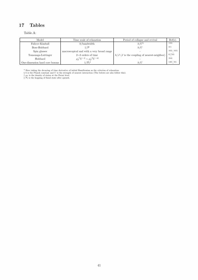
17 Tables
Table.A:
Model Time scale of relaxation Period of collapse and revival Ref(s).
Falicov-Kimball ~/bandwidth h/U § 116)
Bose-Hubbard 1/P h/U 41)
Spin glasses macroscopical and with a very broad range - 162),163)
Tomonaga-Luttinger 2∼3 orders of time h/J (J is the coupling of nearest-neighbor) 6)*,33)
Hubbard ρ−1F U−2 ∼ ρ−3
F U−4† - 164)
One-dimension hard core bosons 1/Pf‡ h/U 148),33)
* Here taking the decaying of time derivative of initial Hamiltonian as the criterion of relaxation.§ h is the Planck constant and U is the strength of nearest interaction (The belows are also follow this).† ρF is the density of states at the Fermi level.‡ Pf is the hopping of finial state after quench.
41
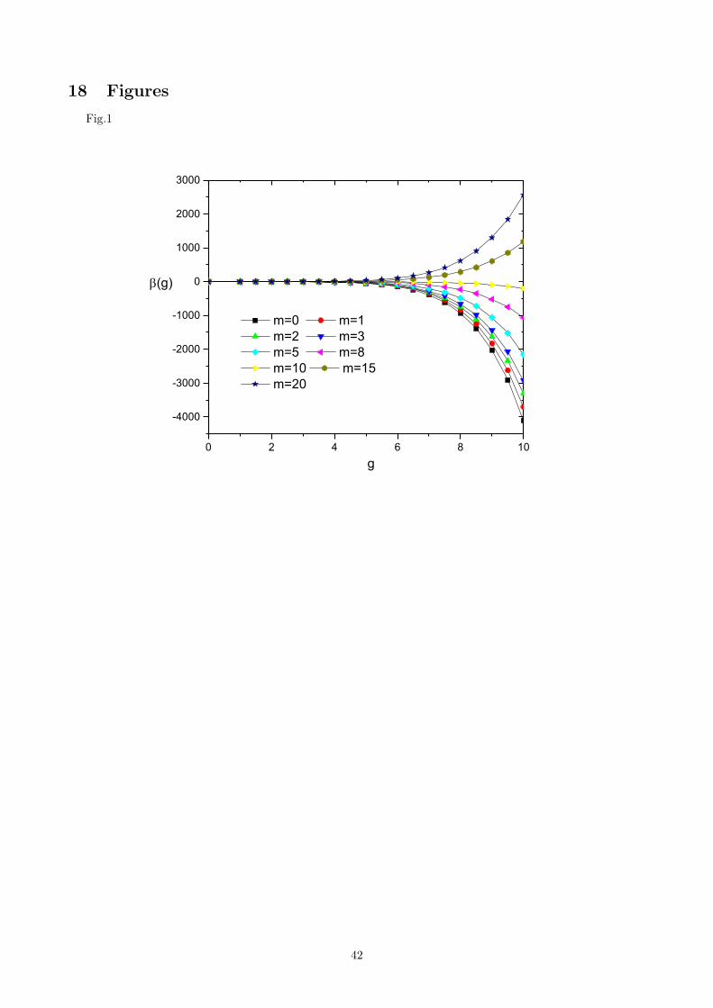
18 Figures
Fig.1
0 2 4 6 8 10
-4000
-3000
-2000
-1000
0
1000
2000
3000
m=0 m=1 m=2 m=3 m=5 m=8 m=10 m=15 m=20
g
(g)
42
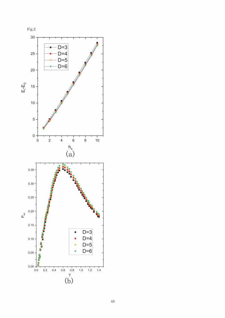
Fig.2
43

Fig.3
44

Fig.4
0.0 0.1 0.2 0.3 0.4 0.5 0.6 0.7
0.00
0.02
0.04
0.06
0.08
0.10
J2=0.6 J2=0.5 J2=0.4 J2=0.3 J2=0.2
C
T
Fig.5
0.0 0.2 0.4 0.6 0.8 1.0 1.2 1.4
0.00
0.05
0.10
0.15
0.20
0.25
S=1 S=1/2
C
T
45
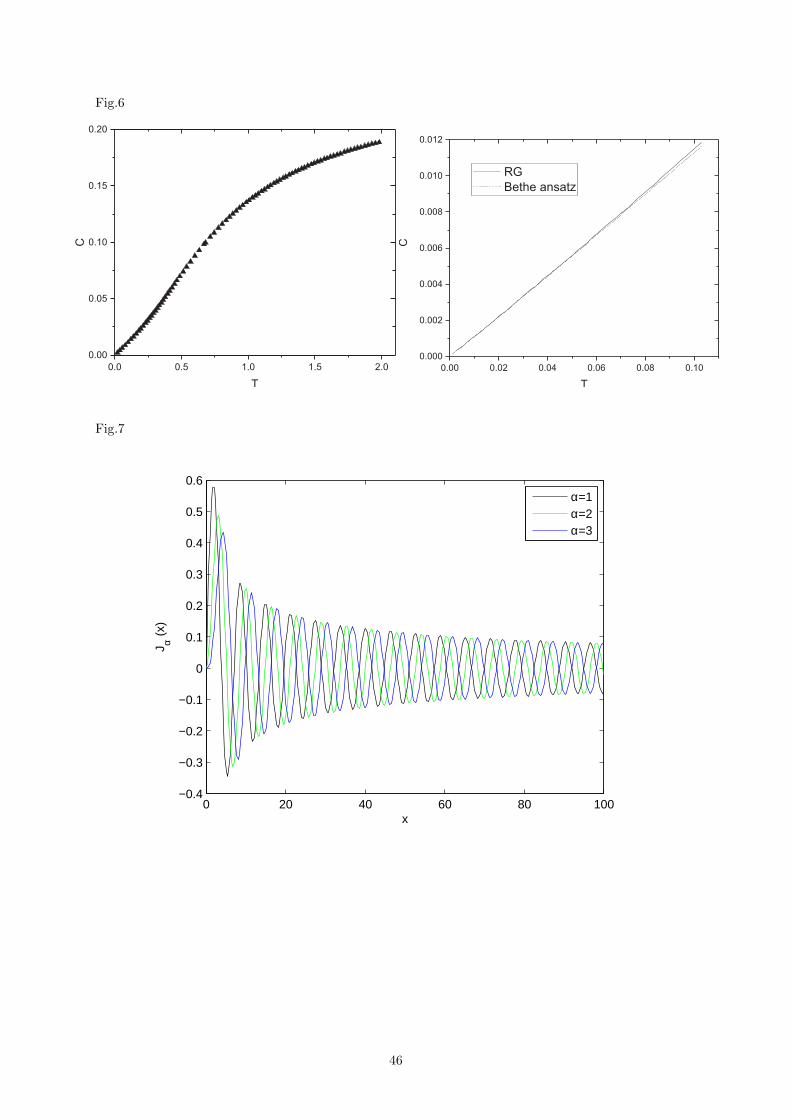
Fig.6
Fig.7
0 20 40 60 80 100−0.4
−0.3
−0.2
−0.1
0
0.1
0.2
0.3
0.4
0.5
0.6
x
J α (x)
α=1α=2α=3
46
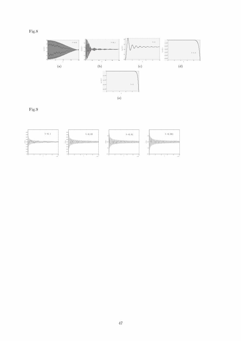
Fig.8
(a) (b) (c) (d)
(e)
Fig.9
0 2 4 6 8 10
x 104
0.2
0.21
0.22
0.23
0.24
0.25
0.26
0.27
0.28
0.29
t
<n
2 (
t)>
0 2 4 6 8 10
x 104
0.2
0.21
0.22
0.23
0.24
0.25
0.26
0.27
0.28
0.29
t
<n
2 (
t)>
0 2 4 6 8 10
x 104
0.15
0.2
0.25
0.3
t
<n
2 (
t)>
0 2 4 6 8 10
x 104
0.15
0.2
0.25
0.3
t
<n
2 (
t)>
47
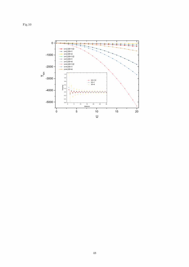
Fig.10
0 5 10 15 20
-5000
-4000
-3000
-2000
-1000
0
0 5 10 15 20 25 30-0.6
-0.4
-0.2
0.0
0.2
0.4
0.6
0.8
1.0T kin
U
n=2,W=1/2 n=2,W=1 n=2,W=4 n=3,W=1/2 n=3,W=1 n=3,W=4 n=4,W=1/2 n=4,W=1 n=4,W=4
hopp
ing
distance
W=1/2 W=1 W=4
48
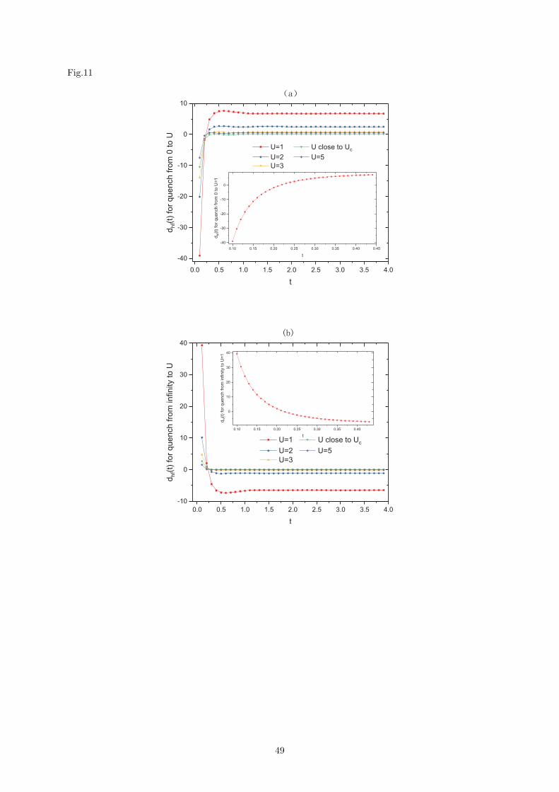
Fig.11
49
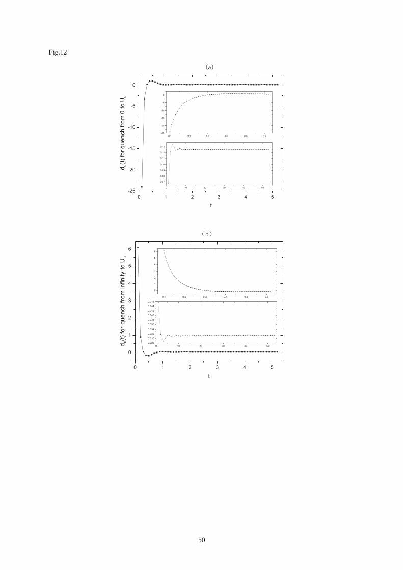
Fig.12
50
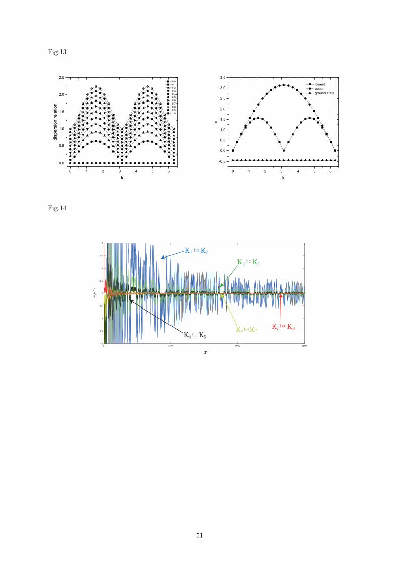
Fig.13
0 1 2 3 4 5 6
0.0
0.5
1.0
1.5
2.0
2.5 0.0 0.1 0.2 0.3 0.4 0.5 0.6 0.7 0.8 0.9 1.0
disp
ersi
on re
latio
n
k0 1 2 3 4 5 6
-0.5
0.0
0.5
1.0
1.5
2.0
2.5
3.0
3.5
k
lowest upper ground state
Fig.14
0 500 1000 1500−2
−1.5
−1
−0.5
0
0.5
1
1.5
2
r
<b0 br +>
51