Embed Size (px)
Citation preview
Project Report
Constraints and Potentials of Diversified Agricultural Development in Eastern India
Project Team
Dr.T.Haque, Director
Council for Social Development New Delhi
Dr. Mondira Bhattacharya,
Associate Fellow Council for Social Development
New Delhi
Mr. Gitesh Sinha, Ms. Purtika Kalra and Mr. Saji Thomas
Research Associates Council for Social Development
New Delhi
Project Sponsored
by Planning Commission (Government of India)
Council for Social Development (CSD) Sangha Rachna, 53 - Lodi Estate,
New Delhi 110003
December 2010
i
ACKNOWLEDGEMENTS
We acknowledge the funding support from the Planning Commission
(Government of India) to Council for Social Development (CSD) for taking up this work
under the project on ‘Constraints and Potentials of Diversified Agricultural Development
in Eastern India’. The team members gratefully acknowledge the support and
encouragement received from Prof. Muchkund Dubey (President, CSD).
We would like to thank Dr. S.S.Sirohi (Joint Director, State Planning Board, Uttar
Pradesh) and Dr. A.K.Roy (Director, Economic Information Technology (EIT), Kolkata,
West Bengal), for undertaking field work in the states of Uttar Pradesh, West Bengal,
Bihar, Jharkhand and Orissa.

ii
TABLE OF CONTENTS
SL. NO. TITLE PAGE NO
ACKNOWLEDGEMENTS (i)
CONTENTS (ii) - (vii)
EXECUTIVE SUMMARY (viii) - (xvi)
CHAPTER 1 INTRODUCTION
1-7
Background
Objectives
Data Base
Secondary Sources of Data
Primary Sources of Data
Methodology
Economic Profile and Production Structure of
Sample Farming Households
Distribution of Farming Households and Land
Holdings
Scheme of Chapterisation
CHAPTER 2 TRENDS AND PATTERNS OF
AGRICULTURAL DIVERSIFICATION
8-80
Share of Gross State Domestic Product from
Agriculture & Allied Activities
Share of Gross State Domestic Product within
Agriculture & Allied Activities
Crop Diversification
Cropping Pattern Changes
District Level Analysis of Cropping Patterns
Inter-Crop Distribution of Gross Value of Crop
Output from Agriculture
Sector wise Distribution of Value of Output in
Agriculture and Allied Activities
Horticultural Diversification
Livestock Diversification
Development of Fisheries
Development of Forestry
Non-Farm Diversification
Agro-Based Industries
Diversification of Exports
CHAPTER 3
PRODUCTION STRUCTURE, PROFITABILITY, INCOME AND VIABILITY
OF SMALL AND MARGINAL FARMS
(RESULTS OF FARM LEVEL SURVEY)
81-110
Share of Farming Households Cultivating Different
Crops
Cropping Pattern
Crop Yields
Livestock Diversification
Diversification towards Fisheries
Viability of Small Farms
iii
CHAPTER 4 CONSTRAINTS, POTENTIALS FOR
AGRICULTURAL DIVERSIFICATION
111-164
Regression Equations
Factors Effecting Value of Output of Agriculture &
Allied Activities (TE – 2006-07)
Factors Effecting Area under Horticultural Crops
and Livestock Population (TE – 1972)
Factors Effecting Area under Horticultural Crops
and Livestock Population (TE – 1982)
Factors Effecting Area under Horticultural Crops
and Livestock Population (TE – 1992)
Factors Effecting Area under Horticultural Crops
and Livestock Population (TE – 2002)
Constraints to Crop Diversification - Based on Field
Survey
Constraints to Fruits Cultivation
Constraints to Vegetables Cultivation
Constraints to Flowers Cultivation
Constraints to Cash Crops Cultivation
Constraints to Livestock Diversification
CHAPTER 5 CONCLUSIONS AND POLICY
IMPLICATIONS 165-176
REFERENCES (xvii) - (xviii)
iv
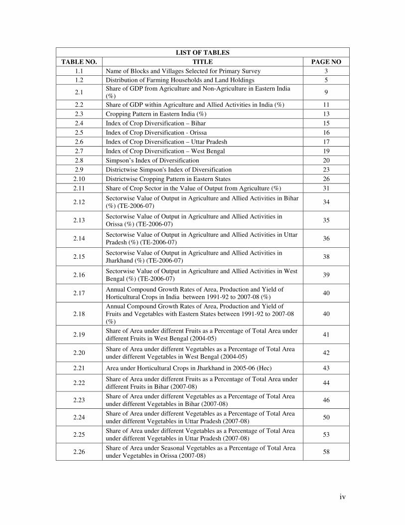
LIST OF TABLES
TABLE NO. TITLE PAGE NO
1.1 Name of Blocks and Villages Selected for Primary Survey 3
1.2 Distribution of Farming Households and Land Holdings 5
2.1 Share of GDP from Agriculture and Non-Agriculture in Eastern India
(%) 9
2.2 Share of GDP within Agriculture and Allied Activities in India (%) 11
2.3 Cropping Pattern in Eastern India (%) 13
2.4 Index of Crop Diversification – Bihar 15
2.5 Index of Crop Diversification - Orissa 16
2.6 Index of Crop Diversification – Uttar Pradesh 17
2.7 Index of Crop Diversification – West Bengal 19
2.8 Simpson’s Index of Diversification 20
2.9 Districtwise Simpson's Index of Diversification 23
2.10 Districtwise Cropping Pattern in Eastern States 26
2.11 Share of Crop Sector in the Value of Output from Agriculture (%) 31
2.12 Sectorwise Value of Output in Agriculture and Allied Activities in Bihar
(%) (TE-2006-07) 34
2.13 Sectorwise Value of Output in Agriculture and Allied Activities in
Orissa (%) (TE-2006-07) 35
2.14 Sectorwise Value of Output in Agriculture and Allied Activities in Uttar
Pradesh (%) (TE-2006-07) 36
2.15 Sectorwise Value of Output in Agriculture and Allied Activities in
Jharkhand (%) (TE-2006-07) 38
2.16 Sectorwise Value of Output in Agriculture and Allied Activities in West
Bengal (%) (TE-2006-07) 39
2.17 Annual Compound Growth Rates of Area, Production and Yield of
Horticultural Crops in India between 1991-92 to 2007-08 (%) 40
2.18
Annual Compound Growth Rates of Area, Production and Yield of
Fruits and Vegetables with Eastern States between 1991-92 to 2007-08
(%)
40
2.19 Share of Area under different Fruits as a Percentage of Total Area under
different Fruits in West Bengal (2004-05) 41
2.20 Share of Area under different Vegetables as a Percentage of Total Area
under different Vegetables in West Bengal (2004-05) 42
2.21 Area under Horticultural Crops in Jharkhand in 2005-06 (Hec) 43
2.22 Share of Area under different Fruits as a Percentage of Total Area under
different Fruits in Bihar (2007-08) 44
2.23 Share of Area under different Vegetables as a Percentage of Total Area
under different Vegetables in Bihar (2007-08) 46
2.24 Share of Area under different Vegetables as a Percentage of Total Area
under different Vegetables in Uttar Pradesh (2007-08) 50
2.25 Share of Area under different Vegetables as a Percentage of Total Area
under different Vegetables in Uttar Pradesh (2007-08) 53
2.26 Share of Area under Seasonal Vegetables as a Percentage of Total Area
under Vegetables in Orissa (2007-08) 58

v
2.27 Share of Area under different Fruits as a Percentage of Total Area under
different Fruits in Orissa (2007-08) 59
2.28 Livestock Population (Million Nos) 60
2.29 Contribution of Livestock Output in Total Value of Agriculture & Allied
Activities 61
2.30 Annual Growth Rate (Compounded) of Different Livestock in Eastern
States (1992 to 2003) 61
2.31 Changes in the Share of Livestock Sector in the Total Value of Output of
Agriculture & Allied Activities (TE-2002 to TE-2006) 65
2.32 Share of Different Iitems in the Total Value of Livestock Output (TE-
2002 to TE-2006) 66
2.33 Share of Inland and Marine Fish in the Total Value of Fisheries Output
(%) 68
2.34 Changes in the Share of Fisheries Sub-Sector in the Total Value of
Output of Agriculture & Allied Activities (%) 68
2.35 Forest Area as a Proportion of Reported Area in the Eastern States (%) 69
2.36 Share of Forestry and Logging in the Gross State Domestic Product of
Agriculture & Allied Sector at Factor Cost (at Constant Prices) 69
2.37 Changes in the Share of Forestry in the Total Value of Output of
Agricultural & Allied Activities 70
2.38 Share of Various Forest Products in the Total Value of Forestry (%) 70
2.39 Percentage Distribution of Persons Employed (Usual Principal Status +
Usual Subsidiary Status), by Industry Section, Rural India 71
2.40 Percentage Distribution of Persons Employed (Usual Principal Status +
Usual Subsidiary Status), by Industry Section in the Eastern States 72
2.41 Percentage Distribution of persons by household type in Rural Areas
(2007-08) 72
2.42 Monthly Average Household Income in 2002-03 (Rs.) 73
2.43
Average Monthly Iincome from Wages, Farm Business and Non-farm
Business per Farmer Household by Size Class of Land Possessed during
the Agricultural Year 2002-03
74
2.44 Average Monthly Consumption Expenditure per Farmer Household by
Size Class of Land Possessed during the Agricultural Year 2002-03 74
2.45 Average Daily wage / Earnings of Casual Labourers and Regular Wage
earners in Rural India (as of 2007-08) 75
2.46 Annual Growth Rates of Total Output in the Organized Food Processing
Sector 78
2.47 Elasticities of Employment with respect to Net Value Added in the Food
Processing Sub-Sector 78
2.48 Share of Agricultural Vis-à-vis Non-agricultural Exports in India (%) 79
2.49 Share of Commodity Exports in Agriculture (%) 79
3.1 Share of Farming Households Cultivating Different Crops (%) 84
3.2 Cropping Pattern - Percentage Share of each Crop in Gross Cropped
Area 87
3.3 Simpson’s Index of Diversification 90
3.4 Crop Yields 97
3.5 Pattern of Livestock as Percentage of Farming Households 101
3.6 Share of Farm Households engaged in Fisheries (%) 102
3.7 Source of Fisheries Reported by Farming Households (%) 103
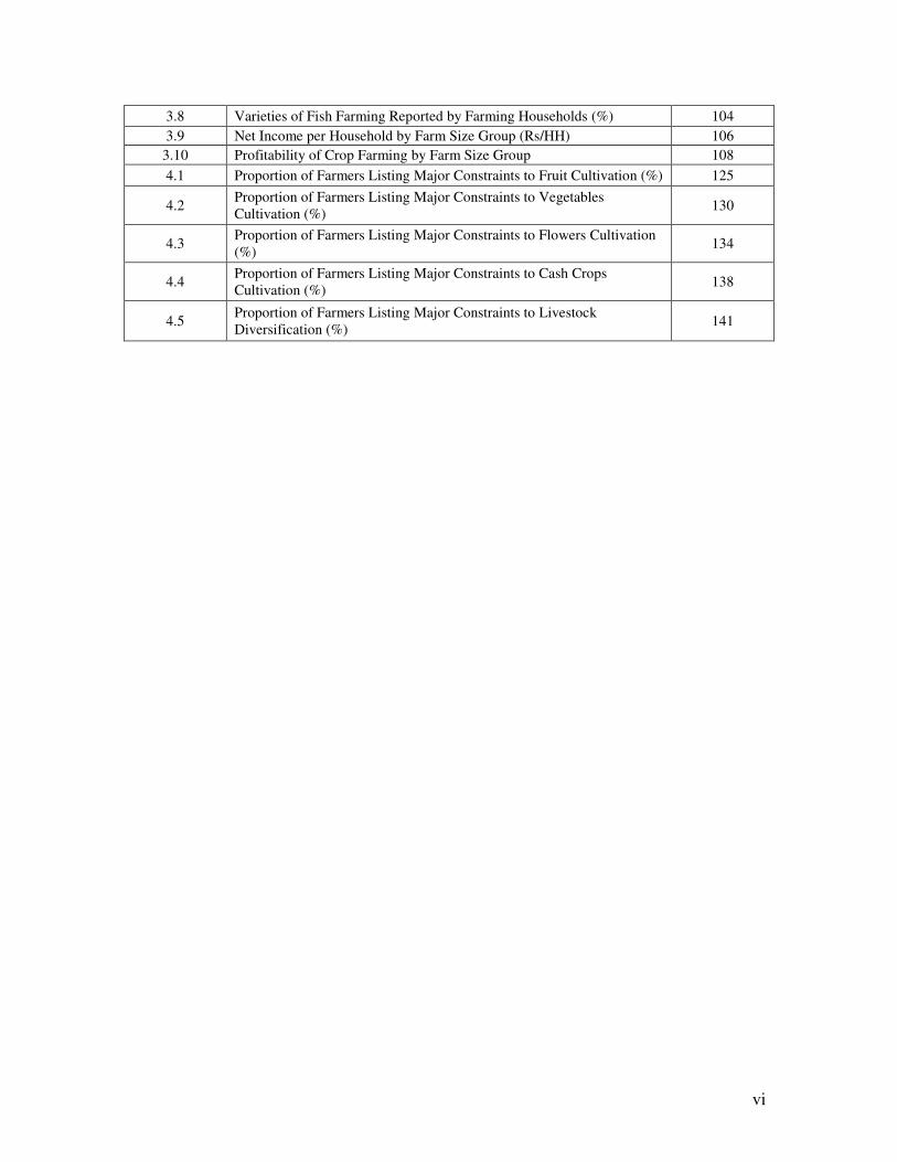
vi
3.8 Varieties of Fish Farming Reported by Farming Households (%) 104
3.9 Net Income per Household by Farm Size Group (Rs/HH) 106
3.10 Profitability of Crop Farming by Farm Size Group 108
4.1 Proportion of Farmers Listing Major Constraints to Fruit Cultivation (%) 125
4.2 Proportion of Farmers Listing Major Constraints to Vegetables
Cultivation (%) 130
4.3 Proportion of Farmers Listing Major Constraints to Flowers Cultivation
(%) 134
4.4 Proportion of Farmers Listing Major Constraints to Cash Crops
Cultivation (%) 138
4.5 Proportion of Farmers Listing Major Constraints to Livestock
Diversification (%) 141
vii
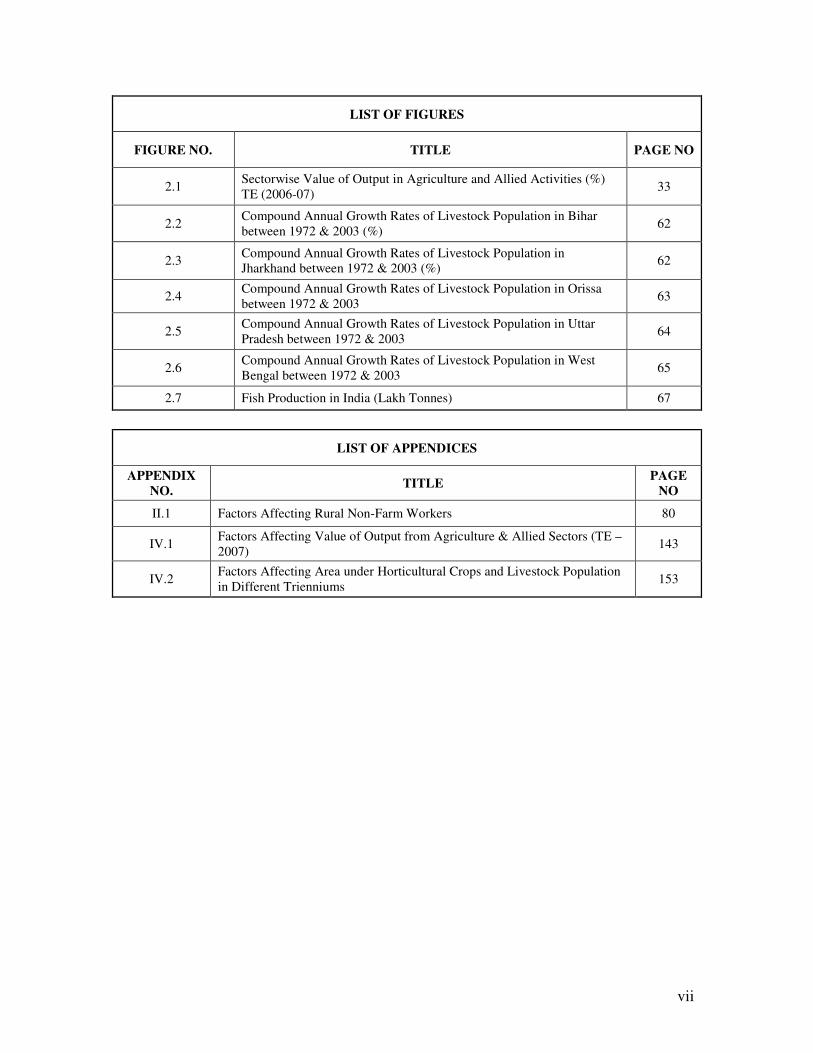
LIST OF FIGURES
FIGURE NO. TITLE PAGE NO
2.1 Sectorwise Value of Output in Agriculture and Allied Activities (%)
TE (2006-07) 33
2.2 Compound Annual Growth Rates of Livestock Population in Bihar
between 1972 & 2003 (%) 62
2.3 Compound Annual Growth Rates of Livestock Population in
Jharkhand between 1972 & 2003 (%) 62
2.4 Compound Annual Growth Rates of Livestock Population in Orissa
between 1972 & 2003 63
2.5 Compound Annual Growth Rates of Livestock Population in Uttar
Pradesh between 1972 & 2003 64
2.6 Compound Annual Growth Rates of Livestock Population in West
Bengal between 1972 & 2003 65
2.7 Fish Production in India (Lakh Tonnes) 67
LIST OF APPENDICES
APPENDIX NO.
TITLE PAGE
NO
II.1 Factors Affecting Rural Non-Farm Workers 80
IV.1 Factors Affecting Value of Output from Agriculture & Allied Sectors (TE –
2007) 143
IV.2 Factors Affecting Area under Horticultural Crops and Livestock Population
in Different Trienniums 153
viii
EXECUTIVE SUMMARY
Introduction/Objectives:
A sustained economic growth, rising per capita income and growing urbanization
are apparently causing a shift in the consumption patterns in favor of high-value food
commodities like fruits, vegetables, dairy, poultry, meat and fish products from staple
food such as rice, wheat and coarse cereals. Such a shift in consumption patterns in favor
of high-value food commodities depicts an on-going process of agricultural
diversification. This study aims to analyze the trends and patterns of agricultural
diversification and related development in the eastern states of India comprising the states
of Bihar, Uttar Pradesh, Jharkhand, Orissa and West Bengal. The reference period of the
study based on secondary data sources has been taken from the period 1970-71 to 2006-
07. Data has also been updated to cover the recent years wherever possible. The primary
survey data pertains to the agricultural year 2010-11.
Objectives
The main objectives of this study were as follows
i) to analyse the trends and patterns of rural diversification, including both
horizontal and vertical diversification in eastern India,
ii) to analyse the constraints and potentials of diversified rural growth in the
different Eastern states, considering various agro-climatic, socio-economic,
technological, infrastructural, institutional and policy factors,
iii) to analyse the various economic aspects including production, profitability,
equity and viability of small and marginal farms in the context of
diversification and lastly
iv) to identify potential sources of diversification and suggest appropriate
strategies and policies for accelerated and diversified agricultural growth as
well as sustainability of small/marginal farms in these regions.
ix
Methodology:
• Database
This study was based on both secondary and primary data, which were collected
and analysed for arriving at results and conclusions. The secondary data at district, state
and national levels for the eastern states were collected from different
departments/agencies/publications relating to different variables/parameters of the study
for the period 1970-71 to 2006-07. The primary data were based on a survey of a cross
section of cultivating households in selected districts of the eastern states. The field study
was undertaken for the agricultural year 2010-11.
• Sampling Technique
The primary data was based on a survey of a cross section of cultivating households in
selected districts of Uttar Pradesh, Bihar, West Bengal, Orissa and Jharkhand. Two
districts from each state were purposively selected – one relatively developed and one
relatively under developed in consultation with district level officers. Further, two blocks
were purposively selected (one relatively developed and one relatively underdeveloped)
from each district and were chosen in consultation with local district level officers. Then
a village or a cluster of villages were chosen from each of the blocks, one again in
consultation with local level officials.
Before the selection of sample farm households, all households were enlisted
along with various information including operational holdings i.e., net cultivated area
(NCA) in the selected villages. Based on the net cultivated area, farm households were
categorized into four broad sub-classes viz., marginal (less than 1 hectare), small
(between 1-2 hectares), medium (2-4 hectares) and large (above 4 hectares). Within sub-
classes, the households were selected based on proportionate random sampling
procedure. Accordingly, 50 households were selected from each village. Thus, making
total sample size of 200 in each of the five states and a grand total of 1000. Following
this, systematic random sampling method was adopted for the selection of sample
households. Under systematic random sampling method, firstly all farm households in a
village were enumerated. The next step was to find the random interval. This was
calculated by dividing the total number of households in particular farm size category
(For e.g. n = 100) in the village by the number of households that are to be selected (e.g.
x
n = 20). Thus, the random interval is equal to 100/20 = 5. Then the first household was
selected using the random numbers table. Subsequently every 5th
household from the total
number of households was taken to frame a sample. Therefore, if the first selected
number was the 5th
household, then the subsequent selected households were the 15th
,
25th
, 35th
, 45th
, and so on. When the random interval was in decimals, it was converted to
the next whole number. However, if a sample household could not be surveyed due to
any reason, then the sampling household with the next sampling serial number was
substituted for collecting information. Farmers were interviewed by using pre-tested
structured schedules.
• Research tools
Agricultural diversification in the eastern states were gauged from share of
various sub-sectors in GDP as well as total value of output from agriculture & allied
activities, sectoral shares in employed persons and cropping pattern. Further two indices
of crop diversification were estimated
(i) Index of Crop Diversification by Bhatia (1965)
(ii) Simpson’s Index of Diversification
At the district level certain factors were taken to explain agricultural
diversification of value of output from crop production, livestock, forestry and fisheries
through multiple regressions using data for the triennium ending 2006-07. These factors
were fertilizer consumption, irrigation, annual rainfall, grazing lands, credit, regulated
markets, village haats, cold storages, rural roads, rural electrification, veterinary
hospitals, forest protection committees, rural literacy and urban population.
Furthermore, factor analysis was undertaken to explain diversification of area and
livestock per 1000 hectares GCA for the trienniums ending 1972-73, 1982-83, 1992-93
and 2002-03. These factors were irrigation, annual rainfall, credit, regulated markets,
rural roads, rural electrification, rural literacy and urban population. In these exercises,
the regressions of Jharkhand could not be formulated due to lack of adequate data under
most heads.
To understand crop diversification, economics of crop production was analysed
for which an analysis of Cost of Cultivation was undertaken. Apart from this, agricultural
diversification in the field was also gauged through horticultural, livestock, fisheries and
xi
non-farm diversification. Data collected through field survey were used extensively for
the detailed analysis which was presented in tabular format. Results of analysis of both
secondary and primary data complement each other to arrive at the conclusions.
Findings/Conclusions:
• Share of Gross State Domestic Product (GSDP) from Agriculture & Allied
Activities
In India the share of GDP from agriculture declined from 35% in 1980-81 to
18.11% in 2007-08, while that of non-agriculture increased from 64.30% to
81.89% in the same period. The eastern states followed the same trend as that of
India. The share of GSDP from agriculture and allied activities in the eastern
region is relatively higher in Uttar Pradesh (29.40%) followed by Bihar (25.34%),
Orissa (22.97%), West Bengal (21.39%) and lastly Jharkhand (9.49%). The share
of GSDP from non-agriculture is very high in Jharkhand (90.51%) followed by
West Bengal (78.61%), Orissa (77.03%), Bihar (74.66%) and lastly Uttar Pradesh
(70.60%). This distribution is on expected lines as Jharkhand, Orissa and West
Bengal have large mineral deposits resulting in large scale industrialization in this
region.
• Cropping Pattern Changes
There has been a significant change in the cropping pattern in the past few
decades. In India as a whole as well in all the eastern states the area share of
cereals in the GCA has been highest amongst other crops from 1970-71 to 2007-
08. It was also observed that the area devoted to food grains (cereals and pulses)
was much higher in all the eastern states compared to horticultural crops. The
proportionate area under horticultural crops was relatively high only in West
Bengal and Bihar.
• Indices of Crop Diversification
The cropping pattern in each state was compared between 1999-2000 and 2006-07
by using the index of crop diversification formulated by Bhatia (1965). It was
seen that crop diversification had reduced from their 1999-2000 levels in the state
of Bihar, Orissa and Jharkhand, while it increased slightly in Uttar Pradesh and a
lot in West Bengal.
xii
From the Simpson’s index of crop diversification (SID), which showed
diversification away from foodgrains, it was seen that in Bihar it increased since
1970-71 but after 2000-01 it showed a decline. In Jharkhand it decreased. In
Orissa it reduced especially since 1995-96. In Uttar Pradesh it increased slightly,
whereas in West Bengal crop diversification away from food grains increased
tremendously. In West Bengal, Orissa and Jharkhand, maximum diversification of
crop was towards oilseeds. In Bihar and Uttar Pradesh, significant crop
diversification was towards plantation crops like jute and sugarcane respectively.
• Inter-crop Distribution of Gross Value of Crop Output from Agriculture
There have also been significant changes in the relative shares of various crops in
the gross value of crop output from agriculture (crop sector) in the past few
decades. In all the eastern states a high proportion of fruits area was under mango.
In West Bengal, a high proportion of vegetables area was under cucurbits and
brinjal. In Bihar and Uttar Pradesh, it was under potato and in Orissa, it was under
rabi vegetables.
It was seen from the analysis of cropping pattern and value of output of
crops that though area diversification away from food grains towards horticultural
crops was increasing over the years in the eastern states but in terms of value of
output, the share of horticultural crops was very high compared to other crops in
all the eastern states except Uttar Pradesh. It is to be noted that Uttar Pradesh is
one of the Green Revolution states and hence cultivation of food grains is very
important here.
• Sector wise Distribution of Value of Output in Agriculture and Allied Activities The sector wise distribution of value of output in agriculture and allied activities
showed that in Bihar the share of livestock was the highest (31.32%). In West
Bengal the share of crop sector was the highest (36.11%). The pattern was similar
in Orissa and Jharkhand. In Uttar Pradesh the share of crop sector was the highest
(59.23%).
xiii
• Sectoral Shares in Employment
In the employment sector, it was seen that the share of employed persons in
agriculture (usual principal status plus usual subsidiary status) in all the eastern
states showed a decline while that of non-agricultural employment increased.
• Field Survey Results
It was observed from the field survey that, sample farming households in the
selected villages of the study regions mainly cultivated cereals, pulses, oilseeds,
vegetables, jute and sugarcane. Cultivation of fruits and flowers was rarely
observed. It was seen that cereals were cultivated by majority households across
all farm size categories in all the states. Further Cereals also occupied a large
proportion of the gross cropped area in all the states.
• The Simpson’s Index of Diversification (SID) was the highest in Orissa (0.25)
followed by Bihar (0.18), West Bengal (0.16), Uttar Pradesh (0.15), and
Jharkhand (0.08). In the states of Orissa, Bihar, West Bengal and Jharkhand the
crop diversification away from food grains was mainly towards oilseeds while in
Uttar Pradesh it was mainly towards sugarcane. Some diversification towards
cultivation of vegetables was observed mainly in the states of Orissa and West
Bengal. From the SID compared using both primary and secondary data it was
seen that the state of Orissa showed more diversification away from food grains
and Jharkhand showed least diversification.
• It was also found that developed districts showed greater crop diversification
away from food grains towards non-food grain crops compared to under
developed districts except for Kishanganj in Bihar and Jalpaiguri in West Bengal
which showed diversification towards oilseeds and jute.
• It was also seen from the field level data that small and marginal farmers showed
more horizontal diversification within the crop sector towards high value crops
such as oilseeds, sugarcane, jute and vegetables compared to the other categories.
Conversely, this category of farmers has shown comparatively lesser horizontal
diversification within the allied sectors such as livestock and fisheries compared
to the other farm sizes.
xiv
• From the pattern of livestock in the study regions it was seen that majority of the
sample farming households owned cattle. The highest proportion of cattle was
seen in West Bengal (70%) followed by Uttar Pradesh (65%), Jharkhand (60%),
Orissa (54%) and Bihar (52%). Higher proportion of poultry was seen in most
underdeveloped districts excepting West Bengal. As regards fisheries, the districts
that showed the highest proportion of farmers who were engaged in fisheries was
Burdwan district of West Bengal (20%) followed by Bhadrak district of Orissa
(11.27%). Most farming households fished from ponds rather than paddy fields.
• Overall it was seen that income from farm sources was more than non-farm
sources in all the selected states of eastern India. The income from non-farm
sources were lesser in the under developed districts compared to the developed
ones. Excepting Jharkhand, the net income from livestock sector was the highest
followed by the agriculture (crop sector) and then the fisheries sector in all the
states. In Jharkhand, the net income from agriculture was the highest followed by
livestock and fisheries sector. Further, the net income from the livestock sector
was greater than the crop sector in all the under developed districts, whereas it
was lesser than the crop sector in all the developed districts, except the Varanasi
district in Uttar Pradesh, where income from the livestock sector was more than
the crop sector.
• Further, it was also seen that despite the fact that small and marginal farmers were
diversifying more within the crop sector into high value crops compared to other
farm size categories, their output-input ratio and income-input ratio were lower
than other farm size categories. Infact their working capital expenses were found
to be relatively higher than other land classes, indicating that these farmers
incurred relatively higher cost of cultivation, but at the same time, they did not
earn commensurate income despite high value crop diversification, indicating
inefficient use of resources by them and also inadequate access to markets for
their high value products.
• From the factor analysis of value of output in agricultural diversification using
districtwise time series data, it was seen that in the state of Bihar unbalanced use
of fertilizers was posing a constraint to horticultural diversification. In the state of
xv
Jharkhand it was found that inappropriate water management and inadequate
water supply was a major constraint towards horticultural diversification.
Moreover, for the fisheries sector poor road conditions, bad road connectivity and
transportation problems in the state were a major problem. In Orissa, livestock
diversification was hindered by road connectivity and transportation problems. In
Orissa, Uttar Pradesh and West Bengal the diversification towards the forestry
sector was mainly constrained by poor rural literacy rates. Further, from the field
level data, the major constraints reported by small and marginal farmers for crop
diversification towards high value crops were lack of proper irrigation facilities,
lack of knowledge and information, and non-availability of timely credit. Further,
in the livestock sector most small and marginal farmers reported lack of access to
veterinary service centres to be a problem.
Recommendations:
• Despite the fact that small and marginal farmers are diversifying horizontally
more within the crop sector compared to the allied sectors, they need to diversify
much more towards high value crops and also within the allied sectors. At the
same time, their resource use efficiency within the crop sector need to improve.
• Further vertical diversification towards non-farm activities was also very less in
the study region and therefore an integrated policy support system is required for
promoting sustainable horizontal and vertical diversification of the rural economy
in eastern India.
• The major constraints reported by small and marginal farmers for crop
diversification towards high value crops were lack of proper irrigation facilities,
lack of knowledge and information, and non-availability of timely credit. Further,
in the livestock sector, most small and marginal farmers reported lack of access to
veterinary service centres to be a problem. Diversification into fisheries sector,
was mostly constrained by lack of timely credit, inaccessibility to cold storages,
poor road conditions and connectivity and transportation problems. Thus, in the
crop, livestock and fisheries sector policies have to be made such that the specific
problems faced by small and marginal farmers can be mitigated. Improving the
xvi
small farmers access to irrigation, credit, technology and veterinary care services
would hold the key in this respect.
• Further, agriculture sector can hardly afford to sustain all its growing population
and therefore vertical diversification especially of small and marginal farms is
necessary. Small and marginal farmers have to be basically part-time farmers. But
the investment and organizational requirements of such vertical diversification in
the form of agro based industries, agri-business, agro-processing and services
would have to be even greater.
• From the factor analysis of value of output in agricultural diversification, it was
seen that in the state of Bihar unbalanced use of fertilizers was posing a constraint
to horticultural diversification. Hence a balanced use of fertilizers was required,
which could be achieved by providing proper training in horticultural
management and practices to farmers. In the state of Jharkhand it was found that
inappropriate water management and inadequate water supply was a major
constraint towards horticultural diversification. Moreover, poor road conditions,
bad road connectivity and transportation problems stood in the way of
development of livestock and fisheries. Therefore, for the fisheries sector poor
road conditions, bad road connectivity and transportation problems in the state
have to be improved. In Orissa, Uttar Pradesh and West Bengal the diversification
towards the forestry sector was mainly constrained by poor rural literacy rates.
Therefore, literacy and awareness building for regeneration and sustainable
management of forest resources would be essential. Also, poor infrastructure of
road and electricity hold back the development of non-farm sector on adequate
scale. Hence development of basic infrastructure, both hard and soft including
road connectivity, electricity, literacy training and skills would be required to help
promote non-farm diversification. Thus, in both the crop as well as the allied
sectors, policies have to be made such that the specific problems faced by farmers
(especially small and marginal) can be mitigated.

1
CHAPTER I
INTRODUCTION
Background
The term ‘diversification’ has been derived from the word ‘diverge’ which means
to move or extend in the direction different from a common point (Jha, Kumar and
Mohanty, 2000). Agricultural diversification can be described in terms of the shift from
the regional dominance of one crop towards the production of a large number of crops to
meet the increasing demand of those crops. It can also be described as the economic
development of non agricultural activities (Start, 2001). The process of diversification
can be classified into horizontal and vertical diversification. Horizontal diversification
can be referred to as that form of diversification wherein farmers diversify their
agricultural activities in order to either stabilize or increase their income or both. It can
either take the form of shift from subsistence farming to commercial farming or the shift
from low value food crops to high value crops. Vertical Diversification refers to the
farmers’ access to non-farm income, i.e., the income from non agricultural sources
(Haque.T, 1996).
A diversified agricultural economy opens up many opportunities. Soil fertility can
be increased by way of crop rotation. It adds value in the agriculture by increasing the
total crop productivity and at the same time stabilizes the farm income by minimizing the
risk associated with only one crop. Since majority of the farmers in India have small
landholdings and their income from crop cultivation as well as non farm income is not
enough to meet their subsistence level and also, the country that produces only a few
specialized crops is more prone to risk due to fluctuations in domestic and international
prices, hence, both the horizontal and vertical diversification become the need of the
hour.
Further, a sustained economic growth, rising per capita income and growing
urbanization are apparently causing a shift in the consumption patterns in favor of high-
value food commodities like fruits, vegetables, dairy, poultry, meat and fish products
from staple food such as rice, wheat and coarse cereals. Such a shift in consumption
2
patterns in favor of high-value food commodities depicts an on-going process of
agricultural diversification. This study basically aims at analysing the trends and patterns
of agricultural diversification and related development in the regions of eastern India.
Objectives
The main objectives of this study are as follows:
i) to analyse the trends and patterns of rural diversification, including both
horizontal and vertical diversification in eastern India comprising the states of
Bihar, Uttar Pradesh, Jharkhand, Orissa and West Bengal;
ii) to analyse the constraints and potentials of diversified rural growth in the
different eastern states, considering various agro-climatic, socio-economic,
technological, infrastructural, institutional and policy factors and
iii) to analyse various economic aspects including production, profitability, equity
and viability of small and marginal farms in the context of diversification.
iv) to identify potential sources and suggest appropriate strategies and policies for
accelerated and diversified agricultural growth as well as sustainability of
small/marginal farms in these areas.
Data Base
Both secondary and primary data were collected and analysed for arriving at
results and conclusions.
Secondary Sources of Data
The secondary data at district, state and national levels for the eastern states were
collected from different departments/agencies/publications relating to different
variables/parameters of the study for the period 1970-71 to 2006-07. Most of the
secondary sources of data were collected from the Directorate of Economics and
Statistics, Department of Agriculture and Cooperation, Ministry of Agriculture,
Government of India, National Sample Survey Rounds of Central Statistical Organisation
(CSO), State Statistical Abstracts, Department of Animal Husbandry & Dairying,
National Horticultural Board and Economic Survey, Government of India.
Primary Sources of Data
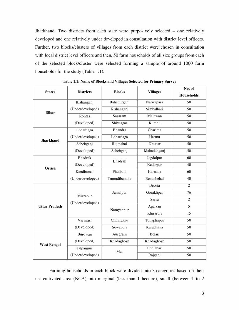
For the purpose of preliminary farm level data, a household survey was conducted
in all five states of eastern India, namely Uttar Pradesh, Bihar, West Bengal, Orissa and
3
Jharkhand. Two districts from each state were purposively selected – one relatively
developed and one relatively under developed in consultation with district level officers.
Further, two blocks/clusters of villages from each district were chosen in consultation
with local district level officers and then, 50 farm households of all size groups from each
of the selected block/cluster were selected forming a sample of around 1000 farm
households for the study (Table 1.1).
Table 1.1: Name of Blocks and Villages Selected for Primary Survey
States Districts Blocks Villages No. of
Households
Bihar
Kishanganj
(Underdeveloped)
Bahadurganj Natwapara 50
Kishanganj Simbalbari 50
Rohtas
(Developed)
Sasaram Malawan 50
Shivsagar Kumhu 50
Jharkhand
Lohardaga
(Underdeveloped)
Bhandra Charima 50
Lohardaga Harmu 50
Sahebganj
(Developed)
Rajmahal Dhutiar 50
Sahebganj Mahadebganj 50
Orissa
Bhadrak
(Developed) Bhadrak
Jagdalpur 60
Kedarpur 40
Kandhamal
(Underdeveloped)
Phulbani Karnada 60
Tumudibandha Benanbehal 40
Uttar Pradesh
Mirzapur
(Underdeveloped)
Jamalpur
Deoria 2
Gorakhpur 76
Sarsa 2
Narayanpur Agarsan 5
Khiraruri 15
Varanasi
(Developed)
Chiraiganu Tohaphapur 50
Sewapuri Karadhana 50
West Bengal
Burdwan
(Developed)
Ausgram Belari 50
Khadaghosh Khadaghosh 50
Jalpaiguri
(Underdeveloped) Mal
Oddlabari 50
Rajganj 50
Farming households in each block were divided into 3 categories based on their
net cultivated area (NCA) into marginal (less than 1 hectare), small (between 1 to 2
4
hectares), medium (between 2 and 4 hectares) and large (above 4 hectares). A detailed
questionnaire schedule was prepared for the collection of primary data.
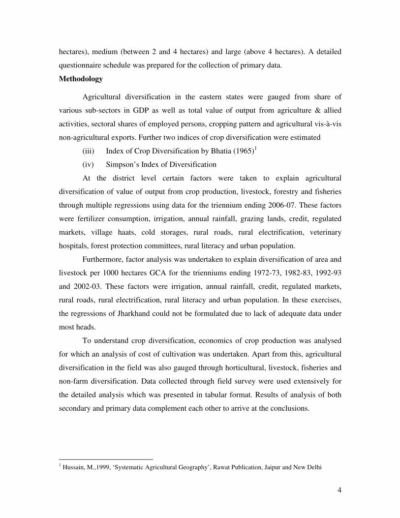
Methodology
Agricultural diversification in the eastern states were gauged from share of
various sub-sectors in GDP as well as total value of output from agriculture & allied
activities, sectoral shares of employed persons, cropping pattern and agricultural vis-à-vis
non-agricultural exports. Further two indices of crop diversification were estimated
(iii) Index of Crop Diversification by Bhatia (1965)1
(iv) Simpson’s Index of Diversification
At the district level certain factors were taken to explain agricultural
diversification of value of output from crop production, livestock, forestry and fisheries
through multiple regressions using data for the triennium ending 2006-07. These factors
were fertilizer consumption, irrigation, annual rainfall, grazing lands, credit, regulated
markets, village haats, cold storages, rural roads, rural electrification, veterinary
hospitals, forest protection committees, rural literacy and urban population.
Furthermore, factor analysis was undertaken to explain diversification of area and
livestock per 1000 hectares GCA for the trienniums ending 1972-73, 1982-83, 1992-93
and 2002-03. These factors were irrigation, annual rainfall, credit, regulated markets,
rural roads, rural electrification, rural literacy and urban population. In these exercises,
the regressions of Jharkhand could not be formulated due to lack of adequate data under
most heads.
To understand crop diversification, economics of crop production was analysed
for which an analysis of cost of cultivation was undertaken. Apart from this, agricultural
diversification in the field was also gauged through horticultural, livestock, fisheries and
non-farm diversification. Data collected through field survey were used extensively for
the detailed analysis which was presented in tabular format. Results of analysis of both
secondary and primary data complement each other to arrive at the conclusions.
1 Hussain, M.,1999, ‘Systematic Agricultural Geography’, Rawat Publication, Jaipur and New Delhi
5
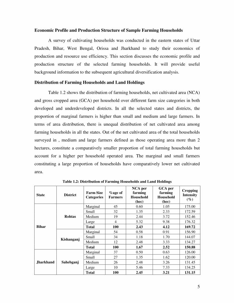
Economic Profile and Production Structure of Sample Farming Households
A survey of cultivating households was conducted in the eastern states of Uttar
Pradesh, Bihar, West Bengal, Orissa and Jharkhand to study their economics of
production and resource use efficiency. This section discusses the economic profile and
production structure of the selected farming households. It will provide useful
background information to the subsequent agricultural diversification analysis.
Distribution of Farming Households and Land Holdings
Table 1.2 shows the distribution of farming households, net cultivated area (NCA)
and gross cropped area (GCA) per household over different farm size categories in both
developed and underdeveloped districts. In all the selected states and districts, the
proportion of marginal farmers is higher than small and medium and large farmers. In
terms of area distribution, there is unequal distribution of net cultivated area among
farming households in all the states. Out of the net cultivated area of the total households
surveyed in , medium and large farmers defined as those operating area more than 2
hectares, constitute a comparatively smaller proportion of total farming households but
account for a higher per household operated area. The marginal and small farmers
constituting a large proportion of households have comparatively lower net cultivated
area.
Table 1.2: Distribution of Farming Households and Land Holdings
State District Farm Size
Categories
%age of
Farmers
NCA per farming
Household
(hec)
GCA per farming
Household
(hec)
Cropping Intensity
(%)
Bihar
Rohtas
Marginal 45 0.60 1.05 175.00
Small 32 1.35 2.33 172.59
Medium 19 2.44 3.72 152.46
Large 4 5.32 9.38 176.32
Total 100 2.43 4.12 169.72
Kishanganj
Marginal 54 0.58 0.91 156.90
Small 34 1.18 1.70 144.07
Medium 12 2.48 3.33 134.27
Total 100 1.67 2.52 150.88
Jharkhand Sahebganj
Marginal 37 0.50 0.63 126.00
Small 27 1.35 1.62 120.00
Medium 26 2.48 3.26 131.45
Large 10 5.46 7.33 134.25
Total 100 2.45 3.21 131.15
6
Lohardaga
Marginal 70 0.44 0.54 122.73
Small 22 1.29 1.45 112.40
Medium 7 2.39 3.18 133.05
Large 1 4.86 4.86 100.00
Total 100 2.25 2.51 111.69
Orissa
Bhadrak
Marginal 47 0.58 0.74 127.59
Small 29 1.27 1.58 124.41
Medium 22 2.24 3.03 135.27
Large 2 4.05 4.86 120.00
Total 100 2.04 2.55 125.43
Kandhamal
Marginal 54 0.55 0.59 107.27
Small 21 1.29 1.36 105.43
Medium 25 2.14 2.49 116.36
Total 100 1.50 1.75 116.25
Uttar
Pradesh
Varanasi
Marginal 44 0.60 1.22 203.33
Small 37 1.31 2.48 189.31
Medium 18 2.47 4.35 176.11
Large 1 4.30 7.63 177.44
Total 100 2.17 3.92 180.65
Mirzapur
Marginal 33 0.74 1.48 200.00
Small 49 1.33 2.65 199.25
Medium 12 2.88 5.76 200.00
Large 6 4.99 9.99 200.20
Total 100 2.49 4.97 200.00
West
Bengal
Burdwan
Marginal 40 0.42 0.75 178.57
Small 30 1.32 1.97 149.24
Medium 25 2.49 3.47 139.36
Large 5 5.60 9.46 168.93
Total 100 2.46 3.91 159.21
Jalpaiguri
Marginal 40 0.36 0.45 125.00
Small 30 1.18 1.44 122.03
Medium 30 2.39 2.95 123.43
Total 100 1.60 2.19 137.03
Source: Primary Field Survey
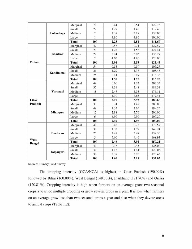
The cropping intensity (GCA/NCA) is highest in Uttar Pradesh (190.99%)
followed by Bihar (160.80%), West Bengal (148.73%), Jharkhand (121.70%) and Orissa
(120.81%). Cropping intensity is high when farmers on an average grow two seasonal
crops a year, do multiple cropping or grow several crops in a year. It is low when farmers
on an average grow less than two seasonal crops a year and also when they devote areas
to annual crops (Table 1.2).

7
Scheme of Chapterisation
Chapter 1: Introduction
Chapter 2: Trends and Patterns of Agricultural Diversification in India
Chapter 3: Production Structure, Profitability and Viability of Small and Marginal Farms
(Results of Farm Level Survey)
Chapter 4: Constraints, Potentials for Agricultural Diversification
Chapter 5: Policy Interventions for Agricultural Diversification
Chapter 6: Conclusions and Policy Implications
8
CHAPTER II
TRENDS AND PATTERNS OF AGRICULTURAL
DIVERSIFICATION
Agriculture and allied activities including crop and animal husbandry, fisheries,
forestry and agro processing provides the basis of our food and livelihood security.
Agriculture and allied activities also provide significant support for economic growth and
social transformation of the country. As one of the world’s largest agrarian economies,
the agriculture sector (including allied activities) in India accounted for 18.11% of the
GDP and contributed approximately 10% of total exports during 2007-08.
Notwithstanding the fact that the share of this sector in the GDP has been declining over
the years, its role remains critical as it provides employment to around 52% of the
workforce. This chapter looks into the trends and patterns of each component of the
agriculture and allied activities sector.
Share of Gross State Domestic Product from Agriculture & Allied Activities
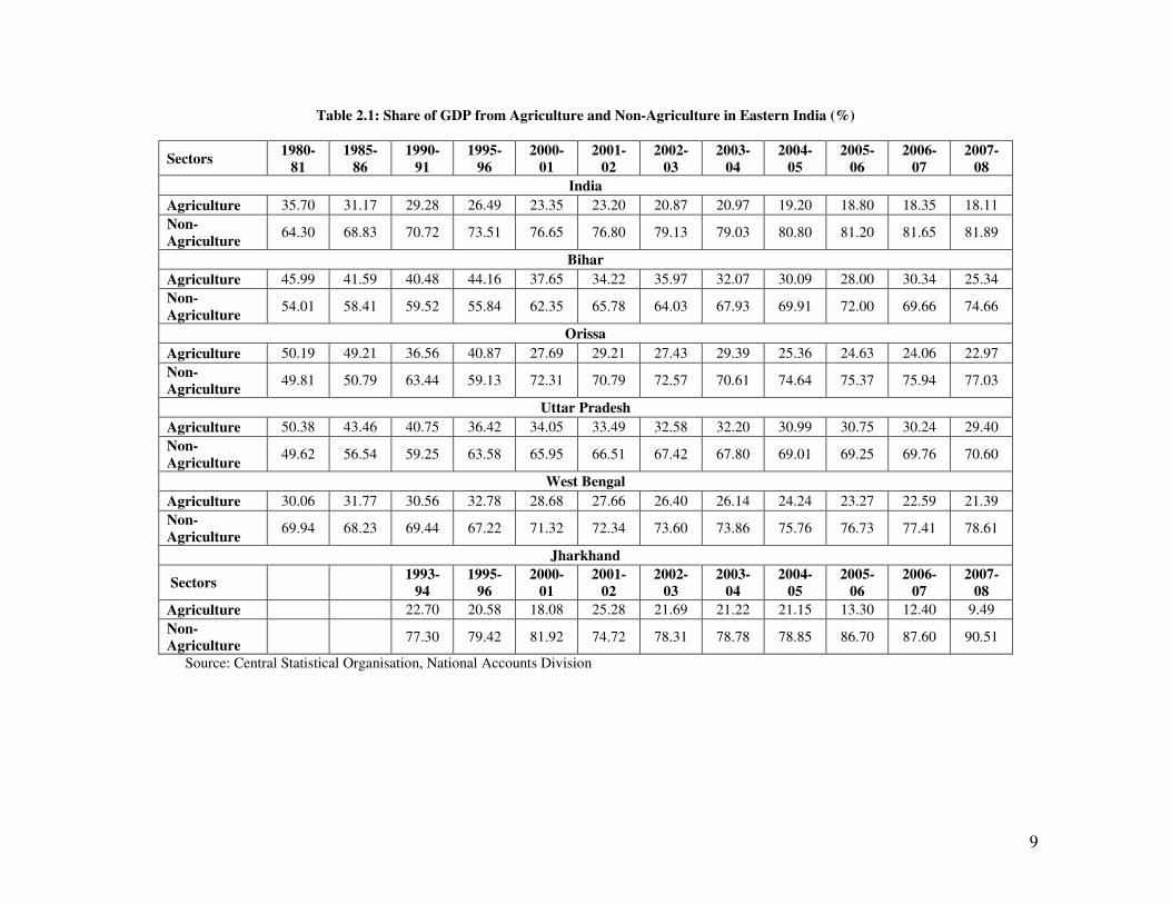
Table 2.1 shows the changes in the shares of agriculture vis-à-vis non-agriculture
in the state domestic product in eastern India. It may be seen from the table that in the
country as a whole, the share of agriculture in the Gross Domestic Product (GDP)
declined from 35% in 1980-81 to 18.11% in 2007-08, while that of non-agriculture
increased from 64.30% to 81.89% in the same period. The eastern states follow the same
trend as that of India. In all the eastern states, the share of agriculture is higher than the
all India level except in Jharkhand in the recent years. Conversely, in all the eastern
states, the share of Gross State Domestic Product (GSDP) from non-agriculture is lower
than the all India level except in Jharkhand in the recent years.
Further, within the eastern region the share of GSDP from agriculture and allied
activities is relatively higher in Uttar Pradesh (29.40%) followed by Bihar (25.34%),
Orissa (22.97%), West Bengal (21.39%) and lastly Jharkhand (9.49%). The share of
GSDP from non-agriculture is very high in Jharkhand (90.51%) followed by West Bengal
(78.61%), Orissa (77.03%), Bihar (74.66%) and lastly Uttar Pradesh (70.60%). This
distribution is on expected lines as Jharkhand, Orissa and West Bengal have large mineral
deposits resulting in large scale industrialization in this region.
9
Table 2.1: Share of GDP from Agriculture and Non-Agriculture in Eastern India (%)
Sectors 1980-
81
1985-
86
1990-
91
1995-
96
2000-
01
2001-
02
2002-
03
2003-
04
2004-
05
2005-
06
2006-
07
2007-
08
India
Agriculture 35.70 31.17 29.28 26.49 23.35 23.20 20.87 20.97 19.20 18.80 18.35 18.11
Non-
Agriculture 64.30 68.83 70.72 73.51 76.65 76.80 79.13 79.03 80.80 81.20 81.65 81.89
Bihar
Agriculture 45.99 41.59 40.48 44.16 37.65 34.22 35.97 32.07 30.09 28.00 30.34 25.34
Non-
Agriculture 54.01 58.41 59.52 55.84 62.35 65.78 64.03 67.93 69.91 72.00 69.66 74.66
Orissa
Agriculture 50.19 49.21 36.56 40.87 27.69 29.21 27.43 29.39 25.36 24.63 24.06 22.97
Non-
Agriculture 49.81 50.79 63.44 59.13 72.31 70.79 72.57 70.61 74.64 75.37 75.94 77.03
Uttar Pradesh
Agriculture 50.38 43.46 40.75 36.42 34.05 33.49 32.58 32.20 30.99 30.75 30.24 29.40
Non-
Agriculture 49.62 56.54 59.25 63.58 65.95 66.51 67.42 67.80 69.01 69.25 69.76 70.60
West Bengal
Agriculture 30.06 31.77 30.56 32.78 28.68 27.66 26.40 26.14 24.24 23.27 22.59 21.39
Non-
Agriculture 69.94 68.23 69.44 67.22 71.32 72.34 73.60 73.86 75.76 76.73 77.41 78.61
Jharkhand
Sectors 1993-
94
1995-
96
2000-
01
2001-
02
2002-
03
2003-
04
2004-
05
2005-
06
2006-
07
2007-
08
Agriculture 22.70 20.58 18.08 25.28 21.69 21.22 21.15 13.30 12.40 9.49
Non-Agriculture
77.30 79.42 81.92 74.72 78.31 78.78 78.85 86.70 87.60 90.51
Source: Central Statistical Organisation, National Accounts Division
10
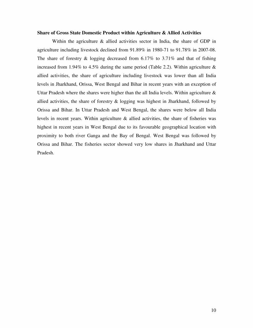
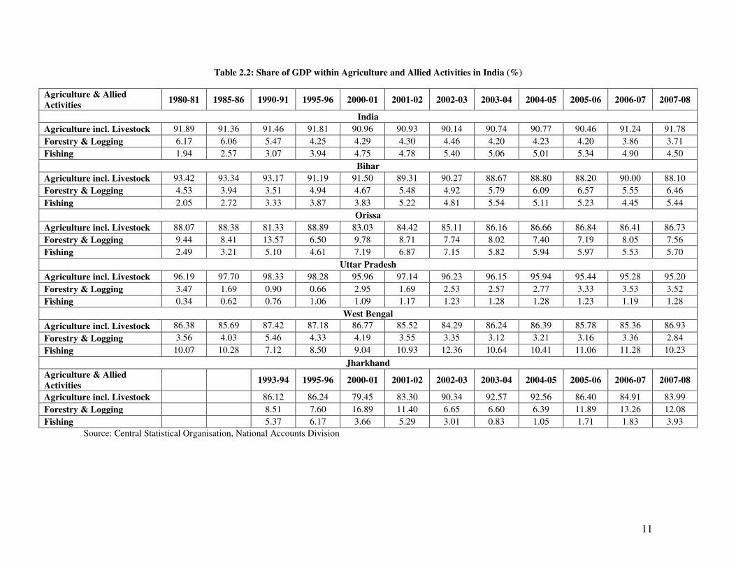
Share of Gross State Domestic Product within Agriculture & Allied Activities
Within the agriculture & allied activities sector in India, the share of GDP in
agriculture including livestock declined from 91.89% in 1980-71 to 91.78% in 2007-08.
The share of forestry & logging decreased from 6.17% to 3.71% and that of fishing
increased from 1.94% to 4.5% during the same period (Table 2.2). Within agriculture &
allied activities, the share of agriculture including livestock was lower than all India
levels in Jharkhand, Orissa, West Bengal and Bihar in recent years with an exception of
Uttar Pradesh where the shares were higher than the all India levels. Within agriculture &
allied activities, the share of forestry & logging was highest in Jharkhand, followed by
Orissa and Bihar. In Uttar Pradesh and West Bengal, the shares were below all India
levels in recent years. Within agriculture & allied activities, the share of fisheries was
highest in recent years in West Bengal due to its favourable geographical location with
proximity to both river Ganga and the Bay of Bengal. West Bengal was followed by
Orissa and Bihar. The fisheries sector showed very low shares in Jharkhand and Uttar
Pradesh.
11
Table 2.2: Share of GDP within Agriculture and Allied Activities in India (%)
Agriculture & Allied
Activities 1980-81 1985-86 1990-91 1995-96 2000-01 2001-02 2002-03 2003-04 2004-05 2005-06 2006-07 2007-08
India
Agriculture incl. Livestock 91.89 91.36 91.46 91.81 90.96 90.93 90.14 90.74 90.77 90.46 91.24 91.78
Forestry & Logging 6.17 6.06 5.47 4.25 4.29 4.30 4.46 4.20 4.23 4.20 3.86 3.71
Fishing 1.94 2.57 3.07 3.94 4.75 4.78 5.40 5.06 5.01 5.34 4.90 4.50
Bihar
Agriculture incl. Livestock 93.42 93.34 93.17 91.19 91.50 89.31 90.27 88.67 88.80 88.20 90.00 88.10
Forestry & Logging 4.53 3.94 3.51 4.94 4.67 5.48 4.92 5.79 6.09 6.57 5.55 6.46
Fishing 2.05 2.72 3.33 3.87 3.83 5.22 4.81 5.54 5.11 5.23 4.45 5.44
Orissa
Agriculture incl. Livestock 88.07 88.38 81.33 88.89 83.03 84.42 85.11 86.16 86.66 86.84 86.41 86.73
Forestry & Logging 9.44 8.41 13.57 6.50 9.78 8.71 7.74 8.02 7.40 7.19 8.05 7.56
Fishing 2.49 3.21 5.10 4.61 7.19 6.87 7.15 5.82 5.94 5.97 5.53 5.70
Uttar Pradesh
Agriculture incl. Livestock 96.19 97.70 98.33 98.28 95.96 97.14 96.23 96.15 95.94 95.44 95.28 95.20
Forestry & Logging 3.47 1.69 0.90 0.66 2.95 1.69 2.53 2.57 2.77 3.33 3.53 3.52
Fishing 0.34 0.62 0.76 1.06 1.09 1.17 1.23 1.28 1.28 1.23 1.19 1.28
West Bengal
Agriculture incl. Livestock 86.38 85.69 87.42 87.18 86.77 85.52 84.29 86.24 86.39 85.78 85.36 86.93
Forestry & Logging 3.56 4.03 5.46 4.33 4.19 3.55 3.35 3.12 3.21 3.16 3.36 2.84
Fishing 10.07 10.28 7.12 8.50 9.04 10.93 12.36 10.64 10.41 11.06 11.28 10.23
Jharkhand
Agriculture & Allied
Activities 1993-94 1995-96 2000-01 2001-02 2002-03 2003-04 2004-05 2005-06 2006-07 2007-08
Agriculture incl. Livestock 86.12 86.24 79.45 83.30 90.34 92.57 92.56 86.40 84.91 83.99
Forestry & Logging 8.51 7.60 16.89 11.40 6.65 6.60 6.39 11.89 13.26 12.08
Fishing 5.37 6.17 3.66 5.29 3.01 0.83 1.05 1.71 1.83 3.93
Source: Central Statistical Organisation, National Accounts Division
12
Crop Diversification
There has been a significant change in the cropping pattern as well as in the
relative share of various crops in the gross value of crop output in the past few decades.
Cropping Pattern Changes
In India as a whole as well in all the eastern states the area share of cereals in the
Gross Cropped Area (GCA) has been highest amongst other crops from 1970-71 to 2007-
08. In India, the area share under cereals in the GCA has declined from 70.30% in 1970-
71 to 61.89% in 2007-08. Area under pulses has reduced marginally. Area under oilseeds
has increased from 9.41% to 13.20%. Area under fruits & vegetables has increased from
0.35% to 1.59%. The area shares of crops like cotton, jute, coconut, sugarcane, and spices
showed a marginal increase during this period (Table 2.3).
In Bihar, the area share of cereals in the GCA has been around 80% in most years
from 1970-71 to 2007-08. Proportionate area under pulses has shown a marginal increase.
The proportion of area under oilseeds and sugarcane declined marginally while
proportion of area under fruits & vegetables and jute & mesta increased slightly over the
years. In Orissa, the area share of cereals in the GCA declined from 68.33% in 1970-71
to 51.35% in 2007-08. However, the area share of cereals started to increase since 1995
but was lower than the levels attained in the 1970s. Proportionate area under pulses
showed substantial increase. The proportion of area under oilseeds, sugarcane, jute &
mesta and fruits & vegetables declined marginally. The area share of sugarcane increased
marginally thereafter. In Uttar Pradesh, the area share of cereals in the GCA increased
marginally from 65.61% in 1970-71 to 67.91% in 2007-08. Proportionate area under
pulses has shown a marginal decline. The proportion of area under oilseeds and
sugarcane increased while that under fruits and vegetables decreased marginally over the
years. In West Bengal, the area share of cereals in the GCA has declined from 74.72% in
1970-71 to 63.27% in 2007-08. Proportionate area under pulses has shown a marginal
decline. The proportion of area under oilseeds increased from 2.07% to 7.25% over the
years while that under fruits & vegetables and jute & mesta increased marginally. The
area share under sugarcane decreased over the years. As regards cropping pattern in
Jharkhand, the area share of cereals in the GCA has declined marginally from 83.72% in
2000-01 to 76.92% in 2007-08. Proportionate area under pulses showed a substantial
13
increase. The proportion of area under jute has shown a marginal decline while that under
fruits & vegetables, oilseeds and sugarcane has shown an increase over the years (Table
2.24).
Table 2.3 also shows that the area devoted to food grains was much higher in all
the eastern states compared to horticultural crops. The proportionate area under
horticultural crops is relatively high only in West Bengal and Bihar.
Table 2.3: Cropping Pattern in Eastern India (%)
Crops 1970-71 1975-76 1980-81 1985-86 1990-91 1995-96 2000-01 2005-06 2007-08
India
Cereals 70.3 70.14 69.97 68.79 66.42 64.46 64.04 61.8 61.89
Pulses 12.75 13.38 12.41 13.12 12.81 11.87 10.77 11.38 11.87
Oilseeds 9.41 9.26 9.72 10.22 12.55 13.83 12.05 14.16 13.2
Cotton 4.3 4.02 4.32 4.05 3.87 4.82 4.51 4.41 4.69
Jute &
Mesta 0.61 0.5 0.72 0.81 0.53 0.5 0.54 0.46 0.48
Coconut 0.59 0.59 0.6 0.66 0.77 0.97 0.97 0.99 1.05
Sugarcane 1.48 1.51 1.47 1.53 1.92 2.21 2.29 2.13 2.51
Fruits &
Vegetables 0.3 0.41 0.54 0.6 0.64 0.8 1.38 1.56 1.59
Spices 0 0 0 0 0 0 0.89 0.77 0.67
Bihar including Jharkhand till 2000-01
Cereals 85 73.58 81.68 77.11 81.11 83 72.36 82.41 81.18
Pulses 7 8.22 8.84 8.34 10.67 9.2 8.97 8.07 7.68
Oilseeds 2.31 2.2 2 1.85 1.98 2.25 1.94 1.88 1.78
Fruits & Vegetables
1.29 1.26 1.28 1.28 2.63 1.48 3.36 3.74 3.61
Sugarcane 2.19 1.24 1.03 1.13 1.02 1.36 1.17 1.37 1.37
Jute 1.47 0.92 1.57 1.91 1.56 1.83 2.09 1.99 1.95
Orissa
Cereals 68.33 66.19 57.42 53.44 48.71 52.9 52.00 51.66 51.35
Pulses 0.85 1.14 1.71 1.97 21.84 9.62 8.00 9.06 9.53
Oilseeds 4.16 4.19 6.94 8.68 7.73 8.81 3.5 3.71 3.58
Fruits &
Vegetables 0.37 0.09 0.1 0.44 0.16 0.18 0.28 0.3 0.3
Sugarcane 0.55 0.59 0.6 0.62 0.51 0.51 0.21 0.18 0.22
Jute 0.65 0.49 0.54 0.6 0.37 0.27 0.35 0.28 0.31
Uttar Pradesh
Cereals 65.61 66.85 71.77 68.63 61.13 62.71 69.58 68.42 67.91
Pulses 11.79 9.74 8.53 8.28 11.13 10.97 10.64 10.87 8.65
Oilseeds 3.1 3.88 3.09 3.56 3.47 6.72 5.63 4.24 5.38
Sugarcane 0.06 0.04 0.04 0.04 0.01 8.08 7.66 8.52 8.74
Fruits &
Vegetables 3.11 3.89 3.11 4.03 3.57 4.17 5.48 4.2 1.27
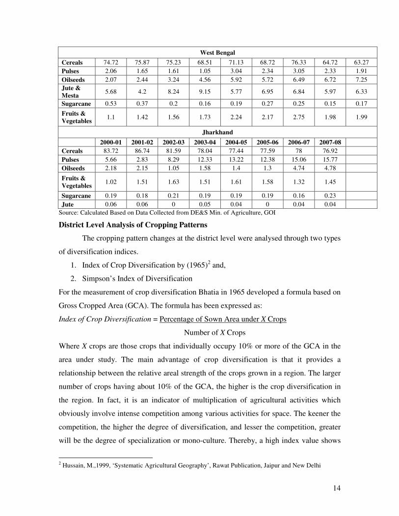
14
West Bengal
Cereals 74.72 75.87 75.23 68.51 71.13 68.72 76.33 64.72 63.27
Pulses 2.06 1.65 1.61 1.05 3.04 2.34 3.05 2.33 1.91
Oilseeds 2.07 2.44 3.24 4.56 5.92 5.72 6.49 6.72 7.25
Jute &
Mesta 5.68 4.2 8.24 9.15 5.77 6.95 6.84 5.97 6.33
Sugarcane 0.53 0.37 0.2 0.16 0.19 0.27 0.25 0.15 0.17
Fruits &
Vegetables 1.1 1.42 1.56 1.73 2.24 2.17 2.75 1.98 1.99
Jharkhand
2000-01 2001-02 2002-03 2003-04 2004-05 2005-06 2006-07 2007-08
Cereals 83.72 86.74 81.59 78.04 77.44 77.59 78 76.92
Pulses 5.66 2.83 8.29 12.33 13.22 12.38 15.06 15.77
Oilseeds 2.18 2.15 1.05 1.58 1.4 1.3 4.74 4.78
Fruits &
Vegetables 1.02 1.51 1.63 1.51 1.61 1.58 1.32 1.45
Sugarcane 0.19 0.18 0.21 0.19 0.19 0.19 0.16 0.23
Jute 0.06 0.06 0 0.05 0.04 0 0.04 0.04
Source: Calculated Based on Data Collected from DE&S Min. of Agriculture, GOI
District Level Analysis of Cropping Patterns
The cropping pattern changes at the district level were analysed through two types
of diversification indices.
1. Index of Crop Diversification by (1965)2 and,
2. Simpson’s Index of Diversification
For the measurement of crop diversification Bhatia in 1965 developed a formula based on
Gross Cropped Area (GCA). The formula has been expressed as:
Index of Crop Diversification = Percentage of Sown Area under X Crops
Number of X Crops
Where X crops are those crops that individually occupy 10% or more of the GCA in the
area under study. The main advantage of crop diversification is that it provides a
relationship between the relative areal strength of the crops grown in a region. The larger
number of crops having about 10% of the GCA, the higher is the crop diversification in
the region. In fact, it is an indicator of multiplication of agricultural activities which
obviously involve intense competition among various activities for space. The keener the
competition, the higher the degree of diversification, and lesser the competition, greater
will be the degree of specialization or mono-culture. Thereby, a high index value shows
2 Hussain, M.,1999, ‘Systematic Agricultural Geography’, Rawat Publication, Jaipur and New Delhi
15
lesser diversification and increased specialization and a low index value shows higher
diversification.3
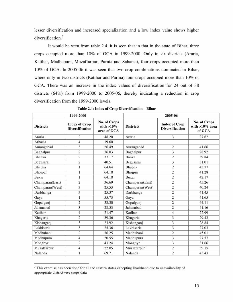
It would be seen from table 2.4, it is seen that in that in the state of Bihar, three
crops occupied more than 10% of GCA in 1999-2000. Only in six districts (Araria,
Katihar, Madhepura, Muzaffarpur, Purnia and Saharsa), four crops occupied more than
10% of GCA. In 2005-06 it was seen that two crop combinations dominated in Bihar,
where only in two districts (Katihar and Purnia) four crops occupied more than 10% of
GCA. There was an increase in the index values of diversification for 24 out of 38
districts (64%) from 1999-2000 to 2005-06, thereby indicating a reduction in crop
diversification from the 1999-2000 levels.
Table 2.4: Index of Crop Diversification – Bihar
1999-2000 2005-06
Districts Index of Crop
Diversification
No. of Crops with >10%
area of GCA
Districts Index of Crop
Diversification
No. of Crops with >10% area
of GCA
Araria 2 48.20 Araria 3 27.62
Arhasia 4 19.60
Aurangabad 3 26.49 Aurangabad 2 41.66
Baghalpur 2 36.03 Baghalpur 3 28.92
Bhanka 2 37.17 Banka 2 39.84
Begusarai 2 40.51 Begusarai 3 31.01
Bhabha 1 64.64 Bhabha 2 43.77
Bhojpur 1 64.18 Bhojpur 2 41.28
Buxar 1 64.18 Buxar 2 42.17
Champaran(East) 2 36.69 Champaran(East) 2 45.26
Champaran(West) 3 25.53 Champaran(West) 2 40.24
Darbhanga 3 25.37 Darbhanga 2 41.45
Gaya 1 55.73 Gaya 2 41.65
Gopalganj 2 38.30 Gopalganj 2 44.11
Jahanabad 3 28.53 Jahanabad 2 41.16
Katihar 4 21.47 Katihar 4 22.99
Khagaria 2 39.36 Khagaria 3 29.43
Kishanganj 3 23.92 Kishanganj 3 28.84
Lakhisaria 3 25.36 Lakhisaria 3 27.03
Madhubani 2 36.25 Madhubani 2 45.01
Madhupura 4 20.55 Madhupura 3 27.57
Monghyr 2 43.24 Monghyr 3 31.66
Muzaffarpur 4 22.05 Muzaffarpur 2 39.15
Nalanda 1 69.71 Nalanda 2 43.43
3 This exercise has been done for all the eastern states excepting Jharkhand due to unavailability of
appropriate districtwise crops data
16
Nawadha 1 71.26 Nawadha 2 44.87
Patna 3 24.83 Patna 3 26.99
Purnia 4 18.39 Purnia 4 22.41
Rohtas 1 76.18 Rohtas 2 45.82
Saharsa 4 22.62 Saharsa 3 28.61
Samastipur 3 23.78 Samastipur 3 29.16
Saran 3 29.31 Saran 3 31.74
Shivhar 2 34.89 Shivhar 2 46.31
Shkhpura 2 39.12 Shkhpura 2 41.17
Sitamarhi 2 36.12 Sitamarhi 2 43.84
Siwan 3 28.89 Siwan 2 43.56
Supaul 2 50.00 Supaul 3 26.70
Vaishali 3 23.65 Vaishali 3 29.18
Zamui 2 36.12 Zamui 2 44.04
Grand Total 3 23.88 Grand Total 2 38.80
Source: Calculated based on the data collected from DE&S Min. of Agriculture, GOI
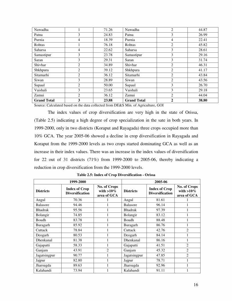
The index values of crop diversification are very high in the state of Orissa,
(Table 2.5) indicating a high degree of crop specialization in the sate in both years. In
1999-2000, only in two districts (Koraput and Rayagada) three crops occupied more than
10% GCA. The year 2005-06 showed a decline in crop diversification in Rayagada and
Koraput from the 1999-2000 levels as two crops started dominating GCA as well as an
increase in their index values. There was an increase in the index values of diversification
for 22 out of 31 districts (71%) from 1999-2000 to 2005-06, thereby indicating a
reduction in crop diversification from the 1999-2000 levels.
Table 2.5: Index of Crop Diversification - Orissa
1999-2000 2005-06
Districts Index of Crop
Diversification
No. of Crops
with >10%
area of GCA
Districts Index of Crop
Diversification
No. of Crops
with >10%
area of GCA
Angul 70.36 1 Angul 81.61 1
Balasore 94.46 1 Balasore 96.14 1
Bhadrak 95.56 1 Bhadrak 97.39 1
Bolangir 74.85 1 Bolangir 83.12 1
Boudh 83.78 1 Boudh 88.48 1
Buragarh 85.92 1 Buragarh 86.76 1
Cuttack 78.84 1 Cuttack 42.76 2
Deogarh 80.53 1 Deogarh 84.14 1
Dhenkanal 81.38 1 Dhenkanal 86.16 1
Gajapatti 58.33 1 Gajapatti 41.51 2
Ganjam 43.91 2 Ganjam 45.32 2
Jagatsingpur 90.77 1 Jagatsingpur 47.85 2
Jajpur 82.80 1 Jajpur 78.71 1
Jharsugda 89.63 1 Jharsugda 92.96 1
Kalahandi 73.94 1 Kalahandi 91.11 1
17
Kandhamal 82.23 1 Kandhamal 83.78 1
Kedrapara 86.68 1 Kedrapara 45.31 2
Keonjhar 80.67 1 Keonjhar 94.99 1
Khurda 47.21 2 Khurda 47.55 2
Koraput 30.00 3 Koraput 46.51 2
Malkangiri 78.71 1 Malkangiri 45.58 2
Mayurbhanj 87.75 1 Mayurbhanj 95.87 1
Nawapara 76.11 1 Nawapara 90.14 1
Naworangpur 66.64 1 Naworangpur 44.68 2
Nayagarh 44.21 2 Nayagarh 44.94 2
Phulbani 49.08 2
Puri 93.23 1 Puri 89.84 1
Rayagada 26.04 3 Rayagada 39.92 2
Sambalpur 88.30 1 Sambalpur 94.08 1
Sonepur 92.10 1 Sonepur 95.55 1
Sundargarh 86.73 1 Sundargarh 94.42 1
Grand Total 80.47 1 Grand Total 85.03 1
Source: Calculated based on the data collected from DE&S Min. of Agriculture, GOI
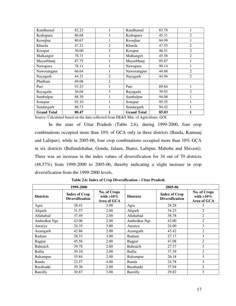
In the state of Uttar Pradesh (Table 2.6), during 1999-2000, four crop
combinations occupied more than 10% of GCA only in three districts (Banda, Kannauj
and Lalitpur), while in 2005-06, four crop combinations occupied more than 10% GCA
in six districts (Bullandshahar, Gonda, Jalaun, Jhansi, Lalitpur, Mahoba and Shivasti).
There was an increase in the index values of diversification for 34 out of 70 districts
(48.57%) from 1999-2000 to 2005-06, thereby indicating a slight increase in crop
diversification from the 1999-2000 levels.
Table 2.6: Index of Crop Diversification – Uttar Pradesh
1999-2000 2005-06
Districts Index of Crop Diversification
No. of Crops
with >10% Area of GCA
Districts Index of Crop Diversification
No. of Crops
with >10% Area of GCA
Agra 28.41 3.00 Agra 28.28 3
Aligarh 31.57 2.00 Aligarh 34.23 2
Allahabad 37.49 2.00 Allahabad 38.78 2
Ambedkar Ngr. 43.06 2.00 Ambedkar Ngr. 43.00 2
Auraiya 24.35 3.00 Auraiya 24.00 3
Azamgarh 42.86 2.00 Azamgarh 43.42 2
Badaun 28.33 3.00 Badaun 27.17 3
Bagpat 45.56 2.00 Bagpat 47.08 2
Bahraich 39.78 2.00 Bahraich 27.37 3
Ballia 39.10 2.00 Ballia 37.39 2
Balrampur 35.84 2.00 Balrampur 26.18 3
Banda 22.57 4.00 Banda 24.78 3
Barabanki 39.36 2.00 Barabanki 37.94 2
Bareilly 30.87 3.00 Bareilly 29.82 3
18
Basti 39.78 2.00 Basti 30.16 3
Bijnor 32.57 3.00 Bijnor 32.40 3
Bullandshahr 25.76 3.00 Bullandshahr 21.52 4
Chandauli 45.60 2.00 Chandauli 43.56 2
Chitrakut 23.54 3.00 Chitrakut 22.39 3
Deoria 42.38 2.00 Deoria 43.57 2
Etah 23.31 3.00 Etah 25.01 3
Etawah 24.87 3.00 Etawah 25.68 3
Faizabad 40.48 2.00 Faizabad 39.91 2
Farrukhabad 23.80 3.00 Farrukhabad 24.31 3
Fatehpur 24.52 3.00 Fatehpur 24.43 3
Firozabad 31.81 2.00 Firozabad 26.40 3
G.Buddha Ngr. 33.82 2.00 G.Buddha Ngr. 39.33 2
Ghaziabad 29.28 3.00 Ghaziabad 40.85 2
Ghazipur 40.32 2.00 Ghazipur 40.00 2
Gonda 27.59 3.00 Gonda 22.44 4
Gorakhpur 44.51 2.00 Gorakhpur 45.14 2
Hamirpur 23.82 3.00 Hamirpur 21.37 3
Hardoi 32.96 2.00 Hardoi 35.33 2
Hatharas 23.96 3.00 Hatharas 26.46 3
J.B.Phule Ngr. 30.12 3.00 J.B.Phule Ngr. 30.00 3
Jalaun 25.67 3.00 Jalaun 18.93 4
Jaunpur 27.65 3.00 Jaunpur 37.62 2
Jhansi 23.61 3.00 Jhansi 21.05 4
Kannauj 20.65 4.00 Kannauj 25.13 3
Kanpur City 26.23 2.00 Kanpur City 28.51 2
Kanpur Dehat 100.00 1.00 Kanpur Dehat 28.34 2
Kaushambi 22.30 3.00 Kaushambi 31.98 2
Kheri 29.94 3.00 Kheri 29.34 3
Kushi Ngr. 31.24 3.00 Kushi Ngr. 30.96 3
Lalitpur 19.42 4.00 Lalitpur 19.11 4
Lucknow 38.33 2.00 Lucknow 39.34 2
Maharahganj 45.01 2.00 Maharahganj 43.60 2
Mahoba 23.95 3.00 Mahoba 19.17 4
Mainpuri 26.42 3.00 Mainpuri 27.38 3
Mathura 26.62 3.00 Mathura 27.11 3
Mau 43.41 2.00 Mau 44.56 2
Meerut 41.86 2.00 Meerut 43.72 2
Mirzapur 36.74 2.00 Mirzapur 36.11 2
Moradabad 28.47 3.00 Moradabad 27.58 3
Muzaffarnagar 32.23 3.00 Muzaffarnagar 45.07 2
Pilibhit 32.48 3.00 Pilibhit 32.16 3
Pratapgarh 38.83 2.00 Pratapgarh 39.94 2
Raebareli 38.61 2.00 Raebareli 39.82 2
Rampur 42.83 2.00 Rampur 43.79 2
S.Ravi Das Ngr. 38.15 2.00 S.Ravi Das Ngr. 39.84 2
Saharanpur 31.26 3.00 Saharanpur 31.31 3
Sant Kabir Ngr. 44.03 2.00 Sant Kabir Ngr. 44.80 2
19
Shahjahanpur 40.79 2.00 Shahjahanpur 40.27 2
Shivasti 30.45 3.00 Shivasti 23.49 4
Siddharth Ngr. 44.77 2.00 Siddharth Ngr. 45.97 2
Sitapur 27.39 3.00 Sitapur 26.75 3
Sonbhadra 28.97 2.00 Sonbhadra 31.05 2
Sultanpur 39.79 2.00 Sultanpur 39.92 2
Unnao 36.65 2.00 Unnao 36.36 2
Varanasi 36.81 2.00 Varanasi 39.47 2
Grand Total 32.50 2.00 Grand Total 32.09 2
Source: Calculated based on the data collected from DE&S Min. of Agriculture, GOI
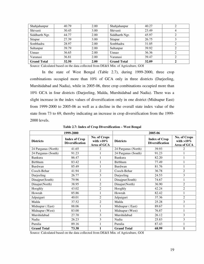
In the state of West Bengal (Table 2.7), during 1999-2000, three crop
combinations occupied more than 10% of GCA only in three districts (Darjeeling,
Murshidabad and Nadia), while in 2005-06, three crop combinations occupied more than
10% GCA in four districts (Darjeeling, Malda, Murshidabad and Nadia). There was a
slight increase in the index values of diversification only in one district (Midnapur East)
from 1999-2000 to 2005-06 as well as a decline in the overall state index value of the
state from 73 to 69, thereby indicating an increase in crop diversification from the 1999-
2000 levels.
Table 2.7: Index of Crop Diversification – West Bengal
1999-2000 2005-06
Districts Index of Crop
Diversification
No. of Crops
with >10%
Area of GCA
Districts Index of Crop
Diversification
No. of Crops
with >10%
Area of GCA
24 Parganas (North) 41.65 2 24 Parganas (North) 39.93 2
24 Parganas (South) 91.23 1 24 Parganas (South) 91.23 1
Bankura 86.47 1 Bankura 82.20 1
Birbhum 83.42 1 Birbhum 77.49 1
Burdwan 85.49 1 Burdwan 81.76 1
Cooch-Behar 41.94 2 Cooch-Behar 36.78 2
Darjeeling 26.77 3 Darjeeling 24.53 3
Dinajpur(South) 79.96 1 Dinajpur(South) 74.67 1
Dinajur(North) 38.95 2 Dinajur(North) 36.90 2
Hooghly 43.02 2 Hooghly 42.24 2
Howrah 85.86 1 Howrah 82.42 1
Jalpaiguri 40.01 2 Jalpaiguri 37.36 2
Malda 37.52 2 Malda 25.28 3
Midnapur ( East) 88.06 1 Midnapur ( East) 89.67 1
Midnapur (West) 83.00 1 Midnapur (West) 76.87 1
Murshidabad 27.70 3 Murshidabad 26.12 3
Nadia 26.23 3 Nadia 25.83 3
Purulia 89.16 1 Purulia 87.43 1
Grand Total 73.38 1 Grand Total 68.99 1
Source: Calculated based on the data collected from DE&S Min. of Agriculture, GOI
20
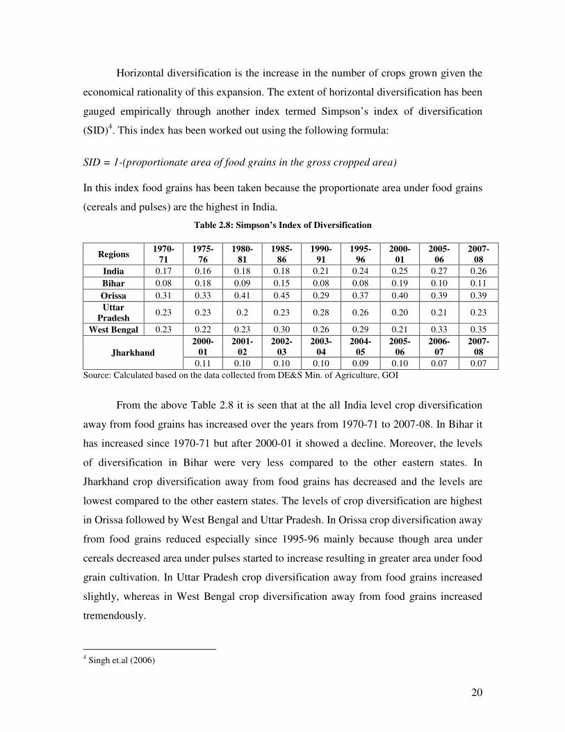
Horizontal diversification is the increase in the number of crops grown given the
economical rationality of this expansion. The extent of horizontal diversification has been
gauged empirically through another index termed Simpson’s index of diversification
(SID)4. This index has been worked out using the following formula:
SID = 1-(proportionate area of food grains in the gross cropped area)
In this index food grains has been taken because the proportionate area under food grains
(cereals and pulses) are the highest in India.
Table 2.8: Simpson’s Index of Diversification
Regions 1970-
71
1975-
76
1980-
81
1985-
86
1990-
91
1995-
96
2000-
01
2005-
06
2007-
08
India 0.17 0.16 0.18 0.18 0.21 0.24 0.25 0.27 0.26
Bihar 0.08 0.18 0.09 0.15 0.08 0.08 0.19 0.10 0.11
Orissa 0.31 0.33 0.41 0.45 0.29 0.37 0.40 0.39 0.39
Uttar
Pradesh 0.23 0.23 0.2 0.23 0.28 0.26 0.20 0.21 0.23
West Bengal 0.23 0.22 0.23 0.30 0.26 0.29 0.21 0.33 0.35
Jharkhand
2000-
01
2001-
02
2002-
03
2003-
04
2004-
05
2005-
06
2006-
07
2007-
08
0.11 0.10 0.10 0.10 0.09 0.10 0.07 0.07
Source: Calculated based on the data collected from DE&S Min. of Agriculture, GOI
From the above Table 2.8 it is seen that at the all India level crop diversification
away from food grains has increased over the years from 1970-71 to 2007-08. In Bihar it
has increased since 1970-71 but after 2000-01 it showed a decline. Moreover, the levels
of diversification in Bihar were very less compared to the other eastern states. In
Jharkhand crop diversification away from food grains has decreased and the levels are
lowest compared to the other eastern states. The levels of crop diversification are highest
in Orissa followed by West Bengal and Uttar Pradesh. In Orissa crop diversification away
from food grains reduced especially since 1995-96 mainly because though area under
cereals decreased area under pulses started to increase resulting in greater area under food
grain cultivation. In Uttar Pradesh crop diversification away from food grains increased
slightly, whereas in West Bengal crop diversification away from food grains increased
tremendously.
4 Singh et.al (2006)
21
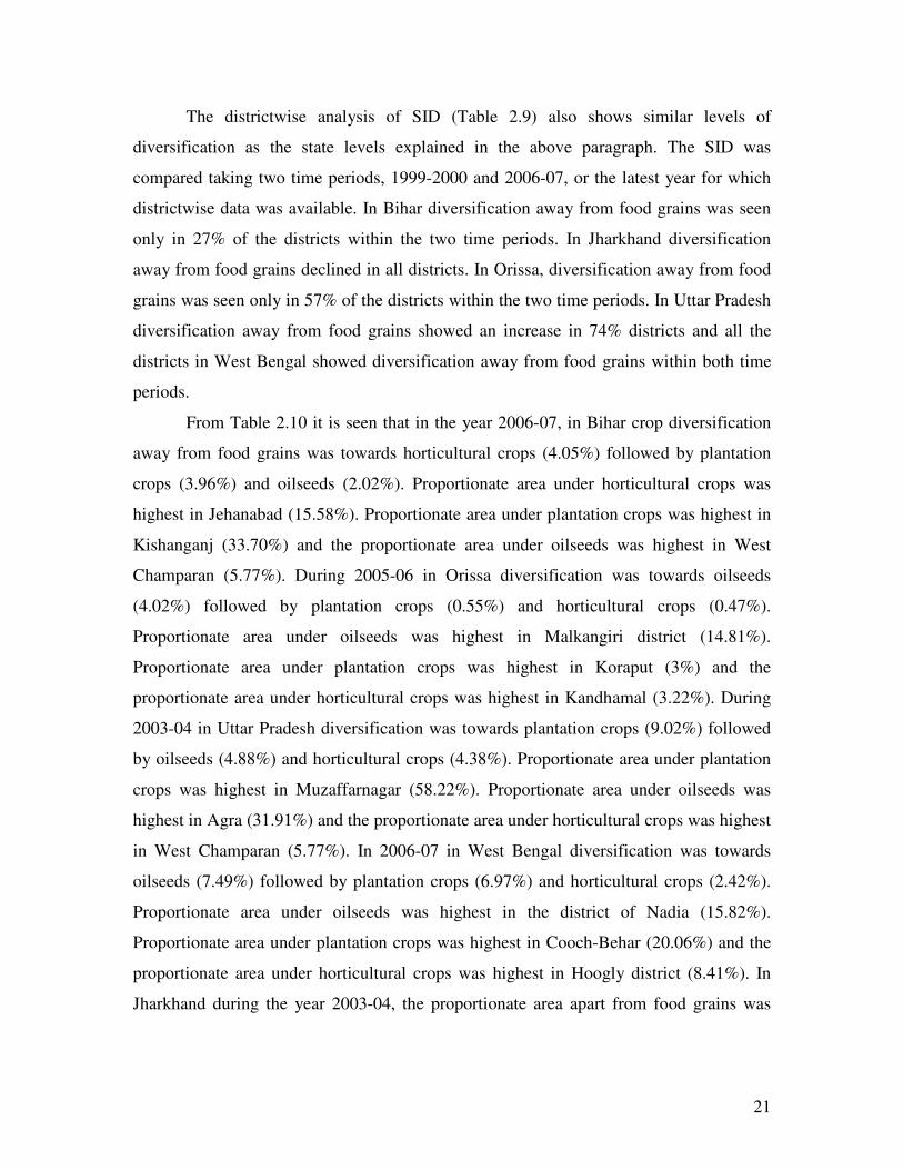
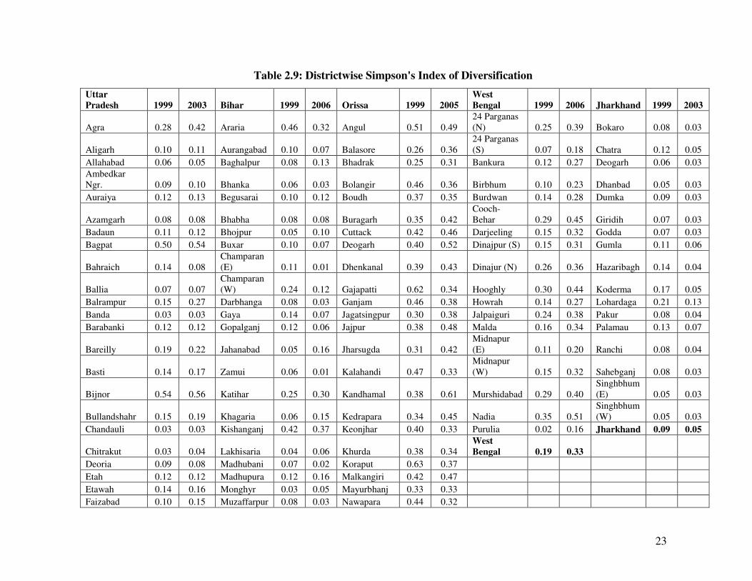
The districtwise analysis of SID (Table 2.9) also shows similar levels of
diversification as the state levels explained in the above paragraph. The SID was
compared taking two time periods, 1999-2000 and 2006-07, or the latest year for which
districtwise data was available. In Bihar diversification away from food grains was seen
only in 27% of the districts within the two time periods. In Jharkhand diversification
away from food grains declined in all districts. In Orissa, diversification away from food
grains was seen only in 57% of the districts within the two time periods. In Uttar Pradesh
diversification away from food grains showed an increase in 74% districts and all the
districts in West Bengal showed diversification away from food grains within both time
periods.
From Table 2.10 it is seen that in the year 2006-07, in Bihar crop diversification
away from food grains was towards horticultural crops (4.05%) followed by plantation
crops (3.96%) and oilseeds (2.02%). Proportionate area under horticultural crops was
highest in Jehanabad (15.58%). Proportionate area under plantation crops was highest in
Kishanganj (33.70%) and the proportionate area under oilseeds was highest in West
Champaran (5.77%). During 2005-06 in Orissa diversification was towards oilseeds
(4.02%) followed by plantation crops (0.55%) and horticultural crops (0.47%).
Proportionate area under oilseeds was highest in Malkangiri district (14.81%).
Proportionate area under plantation crops was highest in Koraput (3%) and the
proportionate area under horticultural crops was highest in Kandhamal (3.22%). During
2003-04 in Uttar Pradesh diversification was towards plantation crops (9.02%) followed
by oilseeds (4.88%) and horticultural crops (4.38%). Proportionate area under plantation
crops was highest in Muzaffarnagar (58.22%). Proportionate area under oilseeds was
highest in Agra (31.91%) and the proportionate area under horticultural crops was highest
in West Champaran (5.77%). In 2006-07 in West Bengal diversification was towards
oilseeds (7.49%) followed by plantation crops (6.97%) and horticultural crops (2.42%).
Proportionate area under oilseeds was highest in the district of Nadia (15.82%).
Proportionate area under plantation crops was highest in Cooch-Behar (20.06%) and the
proportionate area under horticultural crops was highest in Hoogly district (8.41%). In
Jharkhand during the year 2003-04, the proportionate area apart from food grains was
22
mostly under oilseeds (1.67%) and the largest share of area under oilseeds was in
Lohardaga (Table 2.10).
23
Table 2.9: Districtwise Simpson's Index of Diversification
Uttar Pradesh 1999 2003 Bihar 1999 2006 Orissa 1999 2005
West Bengal 1999 2006 Jharkhand 1999 2003
Agra 0.28 0.42 Araria 0.46 0.32 Angul 0.51 0.49
24 Parganas
(N) 0.25 0.39 Bokaro 0.08 0.03
Aligarh 0.10 0.11 Aurangabad 0.10 0.07 Balasore 0.26 0.36
24 Parganas
(S) 0.07 0.18 Chatra 0.12 0.05
Allahabad 0.06 0.05 Baghalpur 0.08 0.13 Bhadrak 0.25 0.31 Bankura 0.12 0.27 Deogarh 0.06 0.03
Ambedkar
Ngr. 0.09 0.10 Bhanka 0.06 0.03 Bolangir 0.46 0.36 Birbhum 0.10 0.23 Dhanbad 0.05 0.03
Auraiya 0.12 0.13 Begusarai 0.10 0.12 Boudh 0.37 0.35 Burdwan 0.14 0.28 Dumka 0.09 0.03
Azamgarh 0.08 0.08 Bhabha 0.08 0.08 Buragarh 0.35 0.42
Cooch-
Behar 0.29 0.45 Giridih 0.07 0.03
Badaun 0.11 0.12 Bhojpur 0.05 0.10 Cuttack 0.42 0.46 Darjeeling 0.15 0.32 Godda 0.07 0.03
Bagpat 0.50 0.54 Buxar 0.10 0.07 Deogarh 0.40 0.52 Dinajpur (S) 0.15 0.31 Gumla 0.11 0.06
Bahraich 0.14 0.08
Champaran
(E) 0.11 0.01 Dhenkanal 0.39 0.43 Dinajur (N) 0.26 0.36 Hazaribagh 0.14 0.04
Ballia 0.07 0.07
Champaran
(W) 0.24 0.12 Gajapatti 0.62 0.34 Hooghly 0.30 0.44 Koderma 0.17 0.05
Balrampur 0.15 0.27 Darbhanga 0.08 0.03 Ganjam 0.46 0.38 Howrah 0.14 0.27 Lohardaga 0.21 0.13
Banda 0.03 0.03 Gaya 0.14 0.07 Jagatsingpur 0.30 0.38 Jalpaiguri 0.24 0.38 Pakur 0.08 0.04
Barabanki 0.12 0.12 Gopalganj 0.12 0.06 Jajpur 0.38 0.48 Malda 0.16 0.34 Palamau 0.13 0.07
Bareilly 0.19 0.22 Jahanabad 0.05 0.16 Jharsugda 0.31 0.42
Midnapur
(E) 0.11 0.20 Ranchi 0.08 0.04
Basti 0.14 0.17 Zamui 0.06 0.01 Kalahandi 0.47 0.33
Midnapur
(W) 0.15 0.32 Sahebganj 0.08 0.03
Bijnor 0.54 0.56 Katihar 0.25 0.30 Kandhamal 0.38 0.61 Murshidabad 0.29 0.40
Singhbhum
(E) 0.05 0.03
Bullandshahr 0.15 0.19 Khagaria 0.06 0.15 Kedrapara 0.34 0.45 Nadia 0.35 0.51
Singhbhum
(W) 0.05 0.03
Chandauli 0.03 0.03 Kishanganj 0.42 0.37 Keonjhar 0.40 0.33 Purulia 0.02 0.16 Jharkhand 0.09 0.05
Chitrakut 0.03 0.04 Lakhisaria 0.04 0.06 Khurda 0.38 0.34 West
Bengal 0.19 0.33
Deoria 0.09 0.08 Madhubani 0.07 0.02 Koraput 0.63 0.37
Etah 0.12 0.12 Madhupura 0.12 0.16 Malkangiri 0.42 0.47
Etawah 0.14 0.16 Monghyr 0.03 0.05 Mayurbhanj 0.33 0.33
Faizabad 0.10 0.15 Muzaffarpur 0.08 0.03 Nawapara 0.44 0.32
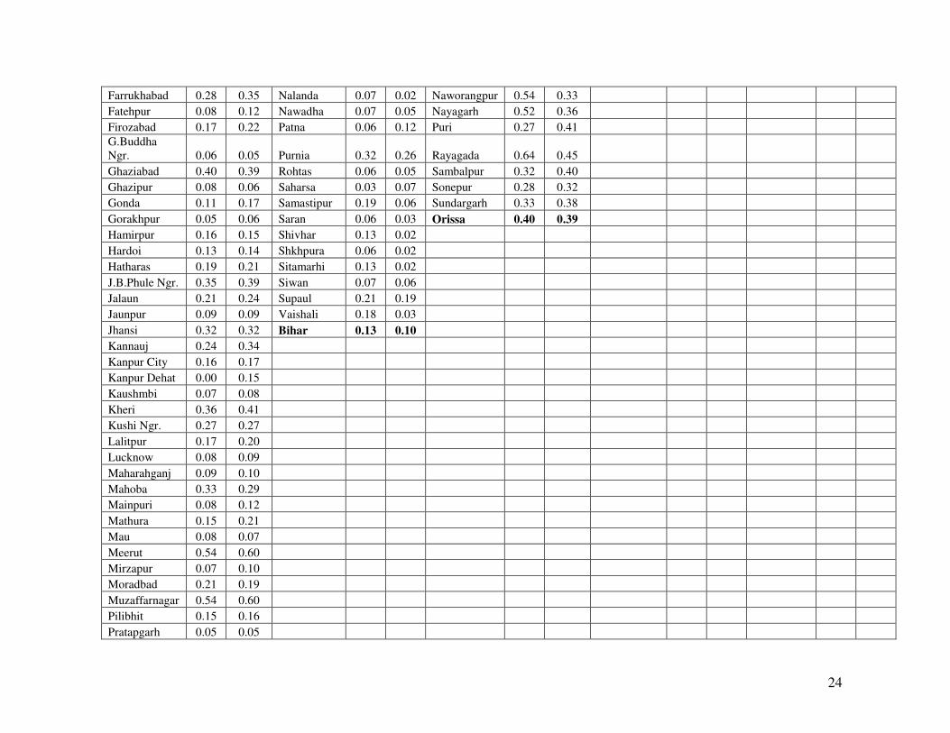
24
Farrukhabad 0.28 0.35 Nalanda 0.07 0.02 Naworangpur 0.54 0.33
Fatehpur 0.08 0.12 Nawadha 0.07 0.05 Nayagarh 0.52 0.36
Firozabad 0.17 0.22 Patna 0.06 0.12 Puri 0.27 0.41
G.Buddha
Ngr. 0.06 0.05 Purnia 0.32 0.26 Rayagada 0.64 0.45
Ghaziabad 0.40 0.39 Rohtas 0.06 0.05 Sambalpur 0.32 0.40
Ghazipur 0.08 0.06 Saharsa 0.03 0.07 Sonepur 0.28 0.32
Gonda 0.11 0.17 Samastipur 0.19 0.06 Sundargarh 0.33 0.38
Gorakhpur 0.05 0.06 Saran 0.06 0.03 Orissa 0.40 0.39
Hamirpur 0.16 0.15 Shivhar 0.13 0.02
Hardoi 0.13 0.14 Shkhpura 0.06 0.02
Hatharas 0.19 0.21 Sitamarhi 0.13 0.02
J.B.Phule Ngr. 0.35 0.39 Siwan 0.07 0.06
Jalaun 0.21 0.24 Supaul 0.21 0.19
Jaunpur 0.09 0.09 Vaishali 0.18 0.03
Jhansi 0.32 0.32 Bihar 0.13 0.10
Kannauj 0.24 0.34
Kanpur City 0.16 0.17
Kanpur Dehat 0.00 0.15
Kaushmbi 0.07 0.08
Kheri 0.36 0.41
Kushi Ngr. 0.27 0.27
Lalitpur 0.17 0.20
Lucknow 0.08 0.09
Maharahganj 0.09 0.10
Mahoba 0.33 0.29
Mainpuri 0.08 0.12
Mathura 0.15 0.21
Mau 0.08 0.07
Meerut 0.54 0.60
Mirzapur 0.07 0.10
Moradbad 0.21 0.19
Muzaffarnagar 0.54 0.60
Pilibhit 0.15 0.16
Pratapgarh 0.05 0.05
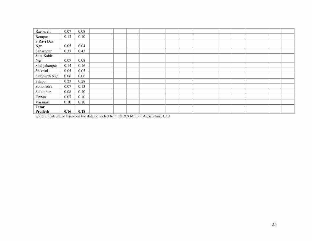
25
Raebareli 0.07 0.08
Rampur 0.12 0.10
S.Ravi Das
Ngr. 0.05 0.04
Saharnpur 0.37 0.43
Sant Kabir
Ngr. 0.07 0.08
Shahjahanpur 0.14 0.16
Shivasti 0.05 0.05
Siddharth Ngr. 0.06 0.06
Sitapur 0.23 0.28
Sonbhadra 0.07 0.13
Sultanpur 0.08 0.10
Unnao 0.07 0.10
Varanasi 0.10 0.10
Uttar
Pradesh 0.16 0.18
Source: Calculated based on the data collected from DE&S Min. of Agriculture, GOI
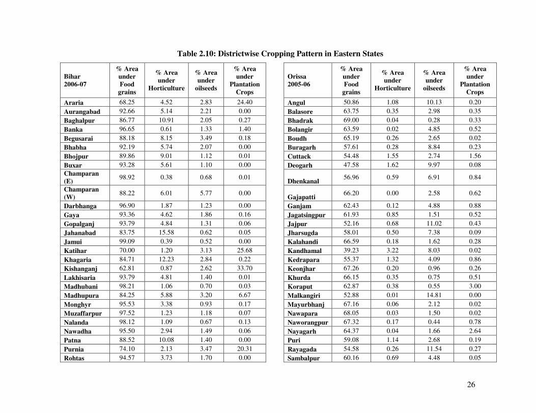
26
Table 2.10: Districtwise Cropping Pattern in Eastern States
Bihar
2006-07
% Area under
Food
grains
% Area
under
Horticulture
% Area
under
oilseeds
% Area under
Plantation
Crops
Orissa
2005-06
% Area under
Food
grains
% Area
under
Horticulture
% Area
under
oilseeds
% Area under
Plantation
Crops
Araria 68.25 4.52 2.83 24.40 Angul 50.86 1.08 10.13 0.20
Aurangabad 92.66 5.14 2.21 0.00 Balasore 63.75 0.35 2.98 0.35
Baghalpur 86.77 10.91 2.05 0.27 Bhadrak 69.00 0.04 0.28 0.33
Banka 96.65 0.61 1.33 1.40 Bolangir 63.59 0.02 4.85 0.52
Begusarai 88.18 8.15 3.49 0.18 Boudh 65.19 0.26 2.65 0.02
Bhabha 92.19 5.74 2.07 0.00 Buragarh 57.61 0.28 8.84 0.23
Bhojpur 89.86 9.01 1.12 0.01 Cuttack 54.48 1.55 2.74 1.56
Buxar 93.28 5.61 1.10 0.00 Deogarh 47.58 1.62 9.97 0.08
Champaran
(E) 98.92 0.38 0.68 0.01
Dhenkanal 56.96 0.59 6.91 0.84
Champaran
(W) 88.22 6.01 5.77 0.00
Gajapatti 66.20 0.00 2.58 0.62
Darbhanga 96.90 1.87 1.23 0.00 Ganjam 62.43 0.12 4.88 0.88
Gaya 93.36 4.62 1.86 0.16 Jagatsingpur 61.93 0.85 1.51 0.52
Gopalganj 93.79 4.84 1.31 0.06 Jajpur 52.16 0.68 11.02 0.43
Jahanabad 83.75 15.58 0.62 0.05 Jharsugda 58.01 0.50 7.38 0.09
Jamui 99.09 0.39 0.52 0.00 Kalahandi 66.59 0.18 1.62 0.28
Katihar 70.00 1.20 3.13 25.68 Kandhamal 39.23 3.22 8.03 0.02
Khagaria 84.71 12.23 2.84 0.22 Kedrapara 55.37 1.32 4.09 0.86
Kishanganj 62.81 0.87 2.62 33.70 Keonjhar 67.26 0.20 0.96 0.26
Lakhisaria 93.79 4.81 1.40 0.01 Khurda 66.15 0.35 0.75 0.51
Madhubani 98.21 1.06 0.70 0.03 Koraput 62.87 0.38 0.55 3.00
Madhupura 84.25 5.88 3.20 6.67 Malkangiri 52.88 0.01 14.81 0.00
Monghyr 95.53 3.38 0.93 0.17 Mayurbhanj 67.16 0.06 2.12 0.02
Muzaffarpur 97.52 1.23 1.18 0.07 Nawapara 68.05 0.03 1.50 0.02
Nalanda 98.12 1.09 0.67 0.13 Naworangpur 67.32 0.17 0.44 0.78
Nawadha 95.50 2.94 1.49 0.06 Nayagarh 64.37 0.04 1.66 2.64
Patna 88.52 10.08 1.40 0.00 Puri 59.08 1.14 2.68 0.19
Purnia 74.10 2.13 3.47 20.31 Rayagada 54.58 0.26 11.54 0.27
Rohtas 94.57 3.73 1.70 0.00 Sambalpur 60.16 0.69 4.48 0.05
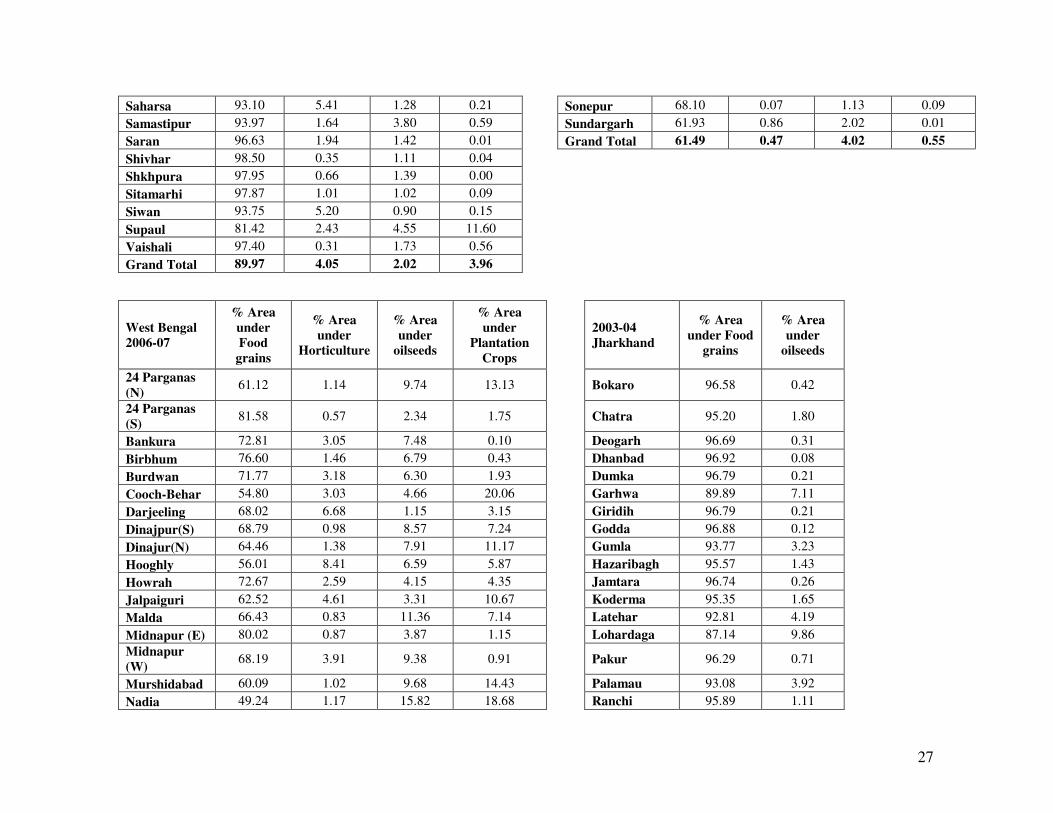
27
Saharsa 93.10 5.41 1.28 0.21 Sonepur 68.10 0.07 1.13 0.09
Samastipur 93.97 1.64 3.80 0.59 Sundargarh 61.93 0.86 2.02 0.01
Saran 96.63 1.94 1.42 0.01 Grand Total 61.49 0.47 4.02 0.55
Shivhar 98.50 0.35 1.11 0.04
Shkhpura 97.95 0.66 1.39 0.00
Sitamarhi 97.87 1.01 1.02 0.09
Siwan 93.75 5.20 0.90 0.15
Supaul 81.42 2.43 4.55 11.60
Vaishali 97.40 0.31 1.73 0.56
Grand Total 89.97 4.05 2.02 3.96
West Bengal 2006-07
% Area
under Food
grains
% Area
under Horticulture
% Area
under oilseeds
% Area
under Plantation
Crops
2003-04 Jharkhand
% Area
under Food grains
% Area
under oilseeds
24 Parganas
(N) 61.12 1.14 9.74 13.13 Bokaro 96.58 0.42
24 Parganas
(S) 81.58 0.57 2.34 1.75 Chatra 95.20 1.80
Bankura 72.81 3.05 7.48 0.10 Deogarh 96.69 0.31
Birbhum 76.60 1.46 6.79 0.43 Dhanbad 96.92 0.08
Burdwan 71.77 3.18 6.30 1.93 Dumka 96.79 0.21
Cooch-Behar 54.80 3.03 4.66 20.06 Garhwa 89.89 7.11
Darjeeling 68.02 6.68 1.15 3.15 Giridih 96.79 0.21
Dinajpur(S) 68.79 0.98 8.57 7.24 Godda 96.88 0.12
Dinajur(N) 64.46 1.38 7.91 11.17 Gumla 93.77 3.23
Hooghly 56.01 8.41 6.59 5.87 Hazaribagh 95.57 1.43
Howrah 72.67 2.59 4.15 4.35 Jamtara 96.74 0.26
Jalpaiguri 62.52 4.61 3.31 10.67 Koderma 95.35 1.65
Malda 66.43 0.83 11.36 7.14 Latehar 92.81 4.19
Midnapur (E) 80.02 0.87 3.87 1.15 Lohardaga 87.14 9.86
Midnapur
(W) 68.19 3.91 9.38 0.91 Pakur 96.29 0.71
Murshidabad 60.09 1.02 9.68 14.43 Palamau 93.08 3.92
Nadia 49.24 1.17 15.82 18.68 Ranchi 95.89 1.11
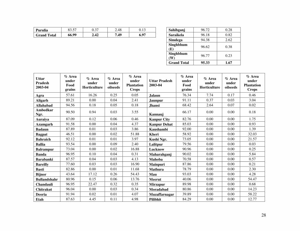
28
Purulia 83.57 0.37 2.48 0.13 Sahibganj 96.72 0.28
Grand Total 66.99 2.42 7.49 6.97 Saraikela 96.18 0.82
Simdega 94.38 2.62
Singhbhum
(E) 96.62 0.38
Singhbhum
(W) 96.77 0.23
Grand Total 95.33 1.67
Uttar
Pradesh
2003-04
% Area
under
Food grains
% Area
under
Horticulture
% Area
under
oilseeds
% Area
under
Plantation Crops
Uttar Pradesh
2003-04
% Area
under
Food grains
% Area
under
Horticulture
% Area
under
oilseeds
% Area
under
Plantation Crops
Agra 57.61 16.26 0.25 0.05 Jalaun 76.34 7.74 0.17 0.46
Aligarh 89.21 0.00 0.04 2.41 Jaunpur 91.11 0.37 0.03 3.04
Allahabad 94.56 0.18 0.05 0.18 Jhansi 68.42 2.64 0.07 0.02
Ambedkar Ngr.
90.50 0.94 0.03 3.55 Kannauj
66.17 0.00 0.00 0.18
Auraiya 87.09 0.12 0.06 0.46 Kanpur City 82.76 0.00 0.00 1.75
Azamgarh 91.58 0.00 0.04 4.37 Kanpur Dehat 85.03 0.00 0.00 0.93
Badaun 87.89 0.01 0.03 3.86 Kaushambi 92.00 0.00 0.00 1.39
Bagpat 46.51 0.00 0.02 51.88 Kheri 58.92 0.00 0.00 32.03
Bahraich 92.12 0.01 0.01 3.97 Kushi Ngr. 73.05 0.00 0.00 21.57
Ballia 93.54 0.00 0.09 2.40 Lalitpur 79.56 0.00 0.00 0.03
Balrampur 73.04 0.00 0.02 16.88 Lucknow 90.96 0.00 0.00 0.25
Banda 96.95 0.10 0.04 0.31 Maharahganj 90.02 0.00 0.00 5.84
Barabanki 87.57 0.04 0.03 4.13 Mahoba 70.58 0.00 0.00 0.57
Bareilly 77.60 0.03 0.03 16.90 Mainpuri 87.86 0.00 0.00 0.21
Basti 82.86 0.00 0.01 11.68 Mathura 78.79 0.00 0.00 2.30
Bijnor 43.64 17.12 0.26 54.43 Mau 93.03 0.00 0.00 4.28
Bullandshahr 80.96 0.15 0.06 13.76 Meerut 40.06 0.00 0.00 54.47
Chandauli 96.95 22.47 0.32 0.35 Mirzapur 89.98 0.00 0.00 0.68
Chitrakut 96.04 0.00 0.03 0.34 Moradabad 80.86 0.00 0.00 14.23
Deoria 91.94 0.02 0.01 4.07 Muzaffarnagar 39.89 0.00 0.00 58.22
Etah 87.63 4.45 0.11 4.98 Pilibhit 84.29 0.00 0.00 12.77
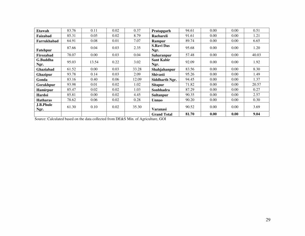
29
Etawah 83.76 0.11 0.02 0.37 Pratapgarh 94.61 0.00 0.00 0.51
Faizabad 85.31 0.05 0.02 8.79 Raebareli 91.61 0.00 0.00 1.21
Farrukhabad 64.91 0.08 0.01 7.07 Rampur 89.74 0.00 0.00 6.65
Fatehpur 87.66 0.04 0.03 2.35
S.Ravi Das
Ngr. 95.68 0.00 0.00 1.20
Firozabad 78.07 0.00 0.03 0.04 Saharanpur 57.48 0.00 0.00 40.03
G.Buddha Ngr.
95.03 13.54 0.22 3.02 Sant Kabir Ngr.
92.09 0.00 0.00 1.92
Ghaziabad 61.52 0.00 0.03 33.28 Shahjahanpur 83.56 0.00 0.00 8.30
Ghazipur 93.78 0.14 0.03 2.09 Shivasti 95.26 0.00 0.00 1.49
Gonda 83.16 0.40 0.06 12.09 Siddharth Ngr. 94.45 0.00 0.00 1.37
Gorakhpur 93.98 0.01 0.02 1.02 Sitapur 71.82 0.00 0.00 20.57
Hamirpur 85.47 0.02 0.02 1.03 Sonbhadra 87.29 0.00 0.00 0.27
Hardoi 85.81 0.00 0.02 4.45 Sultanpur 90.35 0.00 0.00 2.57
Hatharas 78.62 0.06 0.02 0.28 Unnao 90.20 0.00 0.00 0.30
J.B.Phule
Ngr. 61.30 0.10 0.02 35.30
Varanasi 90.52 0.00 0.00 3.69
Grand Total 81.70 0.00 0.00 9.04
Source: Calculated based on the data collected from DE&S Min. of Agriculture, GOI
30
Inter-crop Distribution of Gross Value of Crop Output from Agriculture
At the all India level it is seen that the share of cereals in the value of output from
agriculture is the highest (around 30%) followed closely by fruits & vegetables (around
24%) (Table 2.11). The share of various crops have shown marginal decline over the
years. However the shares of condiments & spices and fruits & vegetables have shown an
increase. In Bihar, the share of food grains especially pulses has shown a sizeable decline
over the years. The shares of other crops especially fruits & vegetables have increased
and is even more than cereal crops, thereby showing diversification towards fruits &
vegetables in Bihar. Jharkhand also shows diversification from cereals toward fruits &
vegetables. All other crops except fibre crops and condiments & spices have shown a
marginal increase in their shares. The shares of fibre crops and condiments & spices
have actually declined in Jharkhand. In Orissa, the share of cereals and fruits &
vegetables showed a significant increase from their 1980-81 levels. The share of
condiments & spices showed marginal increase, while the shares of pulses, oilseeds, fibre
crops and sugarcane showed a decline. In Uttar Pradesh, cereal crops showed higher
share compared to fruits & vegetables and both their shares showed an increase over
time. The shares of pulses and oilseeds have shown a decline whereas those of fibres and
condiments & spices have shown a marginal increase. In West Bengal, the share of
cereals declined over the years, while those of fruits & vegetables increased from their
1980-81 levels. The share of condiments & spices showed marginal increase, while the
rest of crops showed marginal decline.
Thus, it is seen from the analysis of cropping pattern and value of output of crops
that though area diversification away from food grains towards horticultural crops has not
been much over the years in the eastern states but in terms of value of output, the share of
horticultural crops is very high compared to other crops in all the eastern states except
Uttar Pradesh. It is to be noted that Uttar Pradesh is one of the Green Revolution states
and hence cultivation of food grains is very important here.
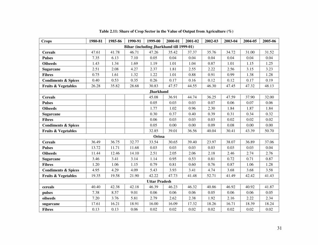
31
Table 2.11: Share of Crop Sector in the Value of Output from Agriculture (%)
Crops 1980-81 1985-86 1990-91 1999-00 2000-01 2001-02 2002-03 2003-04 2004-05 2005-06
Bihar (including Jharkhand till 1999-01)
Cereals 47.61 41.78 46.71 47.26 35.42 37.37 35.76 34.72 31.00 31.52
Pulses 7.35 6.13 7.10 0.05 0.04 0.04 0.04 0.04 0.04 0.04
Oilseeds 1.43 1.34 1.69 1.19 1.01 1.04 0.87 1.01 1.15 1.25
Sugarcane 2.51 2.08 4.27 2.37 1.81 2.55 2.22 2.56 3.15 3.23
Fibres 0.75 1.61 1.32 1.22 1.01 0.88 0.91 0.99 1.38 1.28
Condiments & Spices 0.40 0.53 0.35 0.26 0.17 0.16 0.12 0.12 0.17 0.19
Fruits & Vegetables 26.28 35.82 28.68 30.83 47.57 44.55 46.30 47.45 47.32 48.13
Jharkhand
Cereals 45.08 36.91 44.74 36.25 47.59 37.90 32.00
Pulses 0.05 0.03 0.03 0.07 0.06 0.07 0.06
Oilseeds 1.77 1.02 0.96 2.30 1.84 1.87 1.84
Sugarcane 0.30 0.37 0.40 0.39 0.31 0.34 0.32
Fibres 0.06 0.03 0.03 0.03 0.02 0.02 0.02
Condiments & Spices 0.05 0.00 0.00 0.09 0.08 0.00 0.00
Fruits & Vegetables 32.85 39.01 36.56 40.04 30.41 43.39 50.70
Orissa
Cereals 36.49 36.75 32.77 33.54 30.65 39.40 23.97 38.07 36.89 37.06
Pulses 13.72 11.71 11.68 0.03 0.03 0.03 0.03 0.03 0.03 0.04
Oilseeds 11.44 12.46 14.10 2.51 2.05 2.06 2.18 2.46 2.74 2.76
Sugarcane 3.46 3.41 3.14 1.14 0.95 0.53 0.81 0.72 0.71 0.87
Fibres 1.20 1.06 1.15 0.79 0.81 0.60 0.76 0.87 1.06 1.28
Condiments & Spices 4.95 4.29 4.09 5.43 3.93 3.41 4.74 3.68 3.68 3.58
Fruits & Vegetables 19.35 19.58 21.90 42.22 47.73 41.48 52.71 41.49 42.42 41.43
Uttar Pradesh
cereals 40.40 42.38 42.18 46.39 46.23 46.32 40.86 46.92 40.92 41.87
pulses 7.38 8.57 9.01 0.06 0.06 0.06 0.05 0.06 0.06 0.05
oilseeds 7.20 3.76 5.81 2.79 2.62 2.38 1.92 2.16 2.22 2.34
sugarcane 17.61 16.21 18.91 16.00 16.09 17.32 18.26 16.71 18.39 18.24
Fibres 0.13 0.13 0.06 0.02 0.02 0.02 0.02 0.02 0.02 0.02
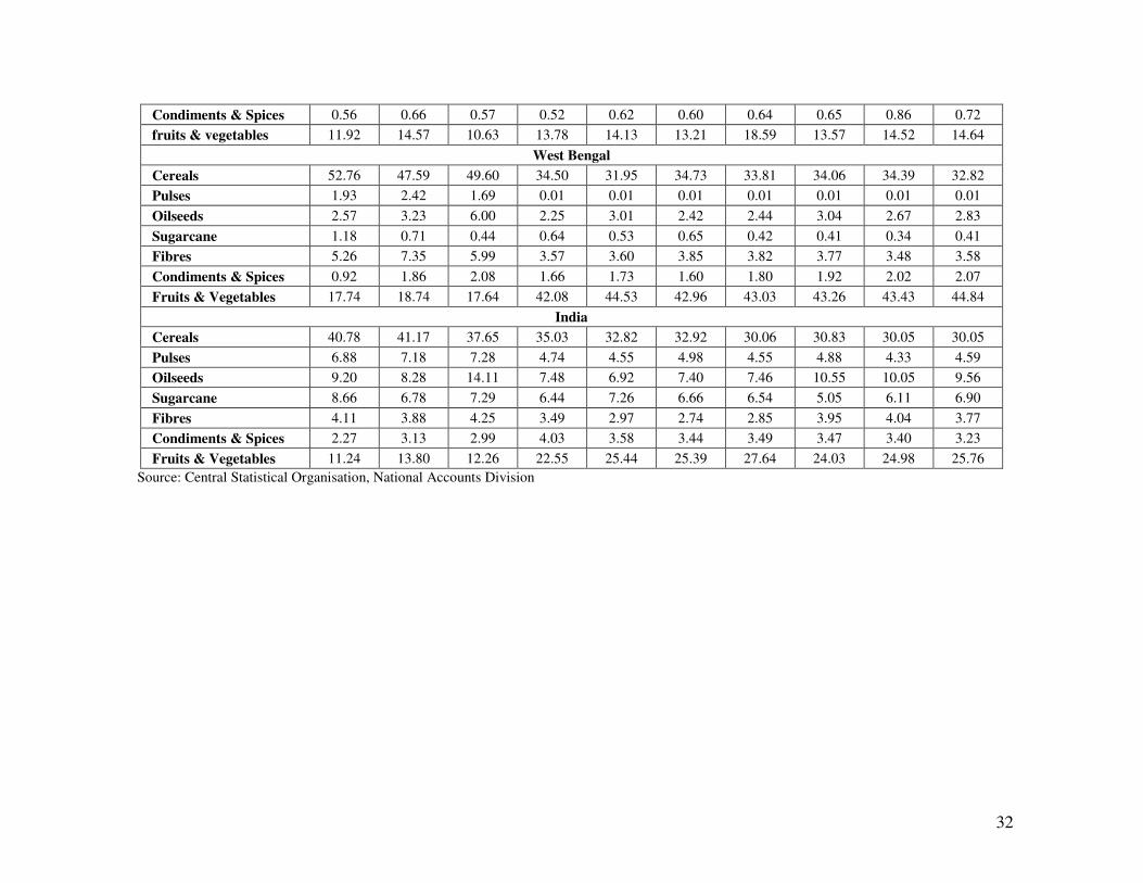
32
Condiments & Spices 0.56 0.66 0.57 0.52 0.62 0.60 0.64 0.65 0.86 0.72
fruits & vegetables 11.92 14.57 10.63 13.78 14.13 13.21 18.59 13.57 14.52 14.64
West Bengal
Cereals 52.76 47.59 49.60 34.50 31.95 34.73 33.81 34.06 34.39 32.82
Pulses 1.93 2.42 1.69 0.01 0.01 0.01 0.01 0.01 0.01 0.01
Oilseeds 2.57 3.23 6.00 2.25 3.01 2.42 2.44 3.04 2.67 2.83
Sugarcane 1.18 0.71 0.44 0.64 0.53 0.65 0.42 0.41 0.34 0.41
Fibres 5.26 7.35 5.99 3.57 3.60 3.85 3.82 3.77 3.48 3.58
Condiments & Spices 0.92 1.86 2.08 1.66 1.73 1.60 1.80 1.92 2.02 2.07
Fruits & Vegetables 17.74 18.74 17.64 42.08 44.53 42.96 43.03 43.26 43.43 44.84
India
Cereals 40.78 41.17 37.65 35.03 32.82 32.92 30.06 30.83 30.05 30.05
Pulses 6.88 7.18 7.28 4.74 4.55 4.98 4.55 4.88 4.33 4.59
Oilseeds 9.20 8.28 14.11 7.48 6.92 7.40 7.46 10.55 10.05 9.56
Sugarcane 8.66 6.78 7.29 6.44 7.26 6.66 6.54 5.05 6.11 6.90
Fibres 4.11 3.88 4.25 3.49 2.97 2.74 2.85 3.95 4.04 3.77
Condiments & Spices 2.27 3.13 2.99 4.03 3.58 3.44 3.49 3.47 3.40 3.23
Fruits & Vegetables 11.24 13.80 12.26 22.55 25.44 25.39 27.64 24.03 24.98 25.76
Source: Central Statistical Organisation, National Accounts Division
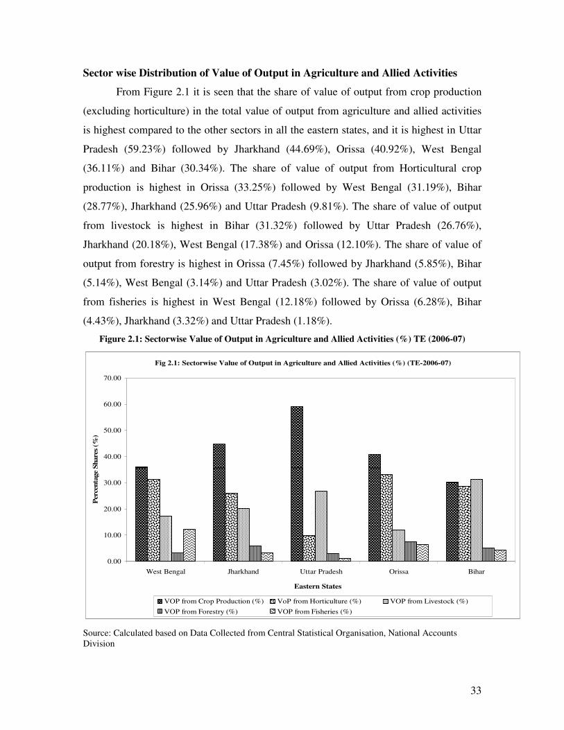
33
Sector wise Distribution of Value of Output in Agriculture and Allied Activities
From Figure 2.1 it is seen that the share of value of output from crop production
(excluding horticulture) in the total value of output from agriculture and allied activities
is highest compared to the other sectors in all the eastern states, and it is highest in Uttar
Pradesh (59.23%) followed by Jharkhand (44.69%), Orissa (40.92%), West Bengal
(36.11%) and Bihar (30.34%). The share of value of output from Horticultural crop
production is highest in Orissa (33.25%) followed by West Bengal (31.19%), Bihar
(28.77%), Jharkhand (25.96%) and Uttar Pradesh (9.81%). The share of value of output
from livestock is highest in Bihar (31.32%) followed by Uttar Pradesh (26.76%),
Jharkhand (20.18%), West Bengal (17.38%) and Orissa (12.10%). The share of value of
output from forestry is highest in Orissa (7.45%) followed by Jharkhand (5.85%), Bihar
(5.14%), West Bengal (3.14%) and Uttar Pradesh (3.02%). The share of value of output
from fisheries is highest in West Bengal (12.18%) followed by Orissa (6.28%), Bihar
(4.43%), Jharkhand (3.32%) and Uttar Pradesh (1.18%).
Figure 2.1: Sectorwise Value of Output in Agriculture and Allied Activities (%) TE (2006-07)
Fig 2.1: Sectorwise Value of Output in Agriculture and Allied Activities (%) (TE-2006-07)
0.00
10.00
20.00
30.00
40.00
50.00
60.00
70.00
West Bengal Jharkhand Uttar Pradesh Orissa Bihar
Eastern States
Per
cen
tage
Sh
are
s (%
)
VOP from Crop Production (%) VoP from Horticulture (%) VOP from Livestock (%)
VOP from Forestry (%) VOP from Fisheries (%)
Source: Calculated based on Data Collected from Central Statistical Organisation, National Accounts
Division

34
In the total value of output from agriculture and allied activities in the state of
Bihar (Table2.12), the share of value of output from livestock is the highest (31.32%)
followed closely by that of crop production (excluding horticulture) (30.34%) and
Horticulture (28.77%). The share of value of output from forestry and fisheries is quite
low, 5.14% and 4.43% respectively. Amongst all states the share of value of output from
crop production was highest in the district of West Champaran (51.47%). Horticulture
showed highest share in Araria (66.20%). The highest share for livestock was seen in
Patna (50.20%). For forestry, highest share was seen in Zamui (41.34%) and for fisheries;
highest share was seen in Saharsa (30.90%)
2.12: Sectorwise Value of Output in Agriculture and Allied Activities in Bihar (%) (TE-2006-07)
Bihar Districts Crop
Production5 Horticulture Livestock Forestry Fisheries
Araria 22.26 66.20 4.37 0.20 6.77
Aurangabad 41.17 8.53 37.71 6.34 0.67
Baghalpur 36.41 17.38 43.40 0.03 2.75
Banka 29.51 12.65 25.59 19.22 0.00
Begusarai 24.29 26.50 26.87 0.00 22.34
Bhabha 26.38 6.32 13.61 35.55 1.24
Bhojpur 39.14 27.33 32.69 0.00 0.85
Buxar 39.01 24.34 26.81 0.00 9.84
Champaran.E 29.35 35.27 34.21 0.02 1.13
Champaran.W 51.47 13.88 14.94 10.94 0.00
Darbhanga 33.00 25.30 41.70 0.00 0.00
Gaya 11.83 15.63 41.16 18.61 0.00
Gopalganj 51.18 21.12 23.70 0.00 4.00
Jahanabad 34.62 16.51 47.98 0.44 0.00
Katihar 27.25 39.43 31.90 0.45 0.52
Khagaria 45.12 21.72 31.03 0.00 2.13
Kishanganj 23.57 34.81 38.21 0.17 3.08
Lakhisaria 33.41 6.61 34.36 14.43 0.40
Madhubani 13.42 41.30 34.99 0.00 10.29
Madhupura 35.99 30.79 25.89 0.00 7.33
Monghyr 19.28 16.30 30.54 20.17 0.31
Muzaffarpur 20.55 31.06 35.24 0.00 13.14
Nalanda 24.45 38.50 34.09 1.48 0.04
Nawadha 15.98 11.92 26.89 26.19 3.70
Patna 17.92 26.10 50.20 0.01 5.76
Purnia 22.02 44.61 29.78 0.02 3.55
Rohtas 40.97 17.02 19.15 12.89 0.02
Saharsa 31.34 12.67 25.09 0.00 30.90
Samastipur 17.32 48.90 29.21 0.00 4.58
5 Excludes value of output from Horticulture
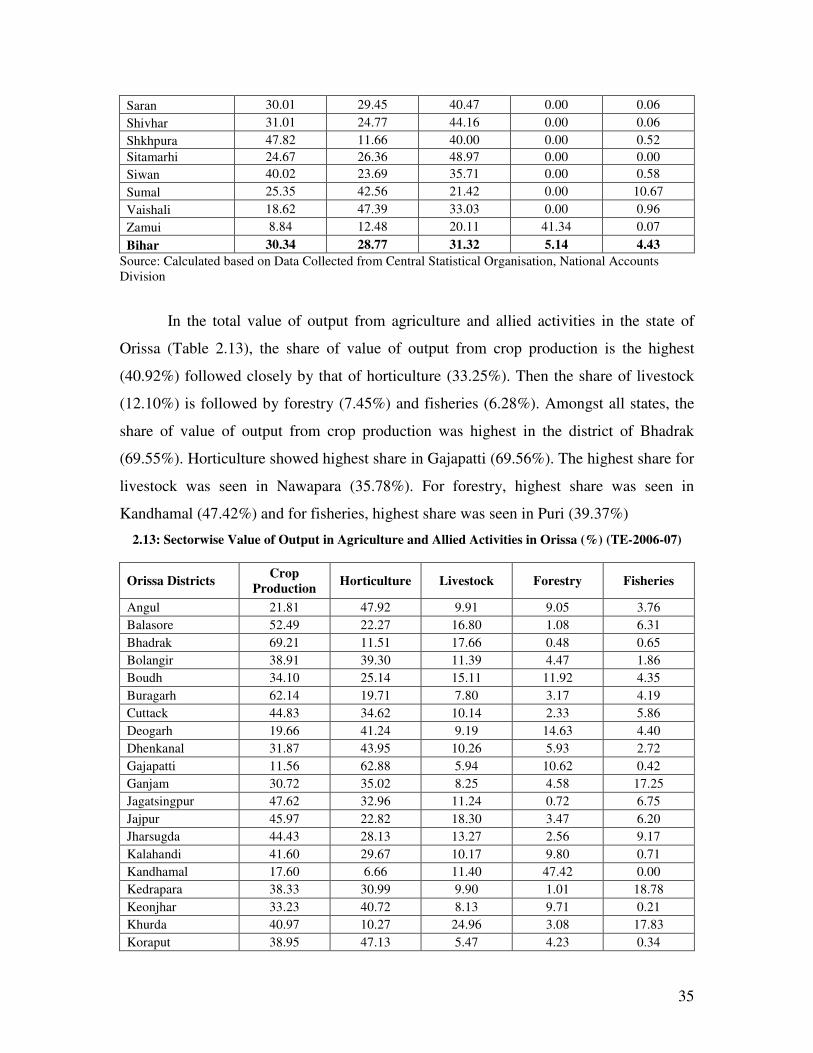
35
Saran 30.01 29.45 40.47 0.00 0.06
Shivhar 31.01 24.77 44.16 0.00 0.06
Shkhpura 47.82 11.66 40.00 0.00 0.52
Sitamarhi 24.67 26.36 48.97 0.00 0.00
Siwan 40.02 23.69 35.71 0.00 0.58
Sumal 25.35 42.56 21.42 0.00 10.67
Vaishali 18.62 47.39 33.03 0.00 0.96
Zamui 8.84 12.48 20.11 41.34 0.07
Bihar 30.34 28.77 31.32 5.14 4.43
Source: Calculated based on Data Collected from Central Statistical Organisation, National Accounts
Division
In the total value of output from agriculture and allied activities in the state of
Orissa (Table 2.13), the share of value of output from crop production is the highest
(40.92%) followed closely by that of horticulture (33.25%). Then the share of livestock
(12.10%) is followed by forestry (7.45%) and fisheries (6.28%). Amongst all states, the
share of value of output from crop production was highest in the district of Bhadrak
(69.55%). Horticulture showed highest share in Gajapatti (69.56%). The highest share for
livestock was seen in Nawapara (35.78%). For forestry, highest share was seen in
Kandhamal (47.42%) and for fisheries, highest share was seen in Puri (39.37%)
2.13: Sectorwise Value of Output in Agriculture and Allied Activities in Orissa (%) (TE-2006-07)
Orissa Districts Crop
Production Horticulture Livestock Forestry Fisheries
Angul 21.81 47.92 9.91 9.05 3.76
Balasore 52.49 22.27 16.80 1.08 6.31
Bhadrak 69.21 11.51 17.66 0.48 0.65
Bolangir 38.91 39.30 11.39 4.47 1.86
Boudh 34.10 25.14 15.11 11.92 4.35
Buragarh 62.14 19.71 7.80 3.17 4.19
Cuttack 44.83 34.62 10.14 2.33 5.86
Deogarh 19.66 41.24 9.19 14.63 4.40
Dhenkanal 31.87 43.95 10.26 5.93 2.72
Gajapatti 11.56 62.88 5.94 10.62 0.42
Ganjam 30.72 35.02 8.25 4.58 17.25
Jagatsingpur 47.62 32.96 11.24 0.72 6.75
Jajpur 45.97 22.82 18.30 3.47 6.20
Jharsugda 44.43 28.13 13.27 2.56 9.17
Kalahandi 41.60 29.67 10.17 9.80 0.71
Kandhamal 17.60 6.66 11.40 47.42 0.00
Kedrapara 38.33 30.99 9.90 1.01 18.78
Keonjhar 33.23 40.72 8.13 9.71 0.21
Khurda 40.97 10.27 24.96 3.08 17.83
Koraput 38.95 47.13 5.47 4.23 0.34
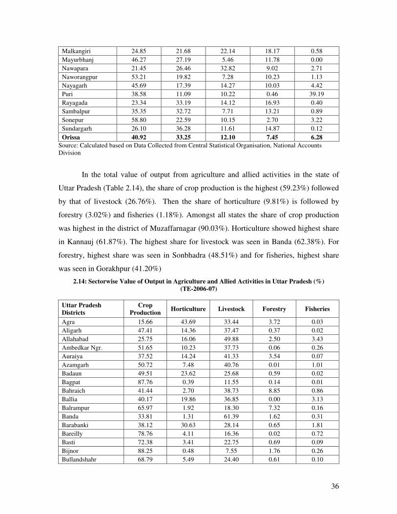
36
Malkangiri 24.85 21.68 22.14 18.17 0.58
Mayurbhanj 46.27 27.19 5.46 11.78 0.00
Nawapara 21.45 26.46 32.82 9.02 2.71
Naworangpur 53.21 19.82 7.28 10.23 1.13
Nayagarh 45.69 17.39 14.27 10.03 4.42
Puri 38.58 11.09 10.22 0.46 39.19
Rayagada 23.34 33.19 14.12 16.93 0.40
Sambalpur 35.35 32.72 7.71 13.21 0.89
Sonepur 58.80 22.59 10.15 2.70 3.22
Sundargarh 26.10 36.28 11.61 14.87 0.12
Orissa 40.92 33.25 12.10 7.45 6.28
Source: Calculated based on Data Collected from Central Statistical Organisation, National Accounts
Division
In the total value of output from agriculture and allied activities in the state of
Uttar Pradesh (Table 2.14), the share of crop production is the highest (59.23%) followed
by that of livestock (26.76%). Then the share of horticulture (9.81%) is followed by
forestry (3.02%) and fisheries (1.18%). Amongst all states the share of crop production
was highest in the district of Muzaffarnagar (90.03%). Horticulture showed highest share
in Kannauj (61.87%). The highest share for livestock was seen in Banda (62.38%). For
forestry, highest share was seen in Sonbhadra (48.51%) and for fisheries, highest share
was seen in Gorakhpur (41.20%)
2.14: Sectorwise Value of Output in Agriculture and Allied Activities in Uttar Pradesh (%)
(TE-2006-07)
Uttar Pradesh
Districts
Crop
Production Horticulture Livestock Forestry Fisheries
Agra 15.66 43.69 33.44 3.72 0.03
Aligarh 47.41 14.36 37.47 0.37 0.02
Allahabad 25.75 16.06 49.88 2.50 3.43
Ambedkar Ngr. 51.65 10.23 37.73 0.06 0.26
Auraiya 37.52 14.24 41.33 3.54 0.07
Azamgarh 50.72 7.48 40.76 0.01 1.01
Badaun 49.51 23.62 25.68 0.59 0.02
Bagpat 87.76 0.39 11.55 0.14 0.01
Bahraich 41.44 2.70 38.73 8.85 0.86
Ballia 40.17 19.86 36.85 0.00 3.13
Balrampur 65.97 1.92 18.30 7.32 0.16
Banda 33.81 1.31 61.39 1.62 0.31
Barabanki 38.12 30.63 28.14 0.65 1.81
Bareilly 78.76 4.11 16.36 0.02 0.72
Basti 72.38 3.41 22.75 0.69 0.09
Bijnor 88.25 0.48 7.55 1.76 0.26
Bullandshahr 68.79 5.49 24.40 0.61 0.10
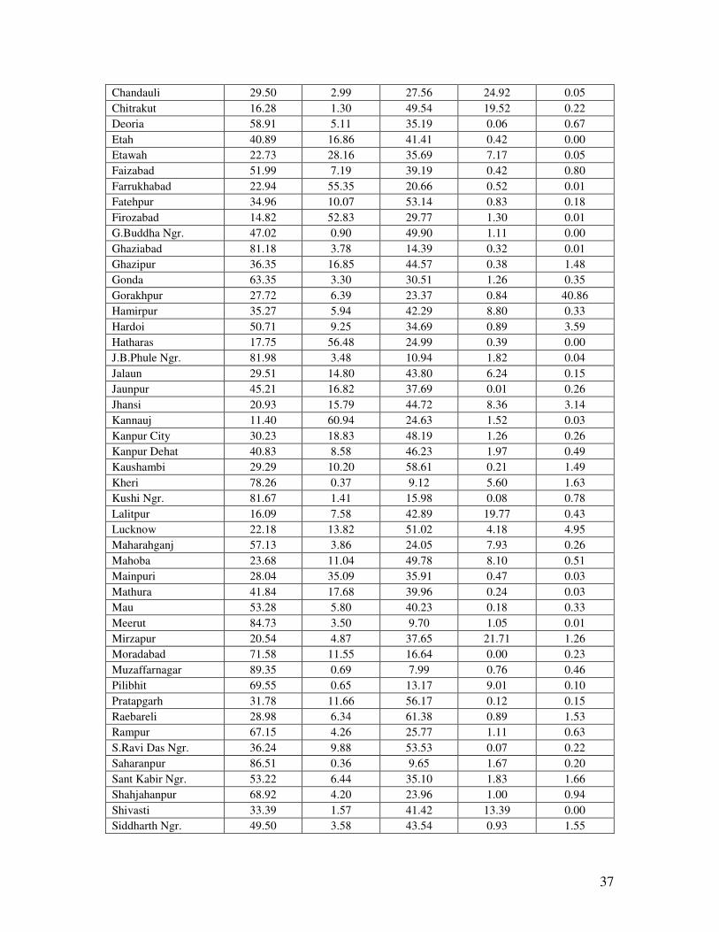
37
Chandauli 29.50 2.99 27.56 24.92 0.05
Chitrakut 16.28 1.30 49.54 19.52 0.22
Deoria 58.91 5.11 35.19 0.06 0.67
Etah 40.89 16.86 41.41 0.42 0.00
Etawah 22.73 28.16 35.69 7.17 0.05
Faizabad 51.99 7.19 39.19 0.42 0.80
Farrukhabad 22.94 55.35 20.66 0.52 0.01
Fatehpur 34.96 10.07 53.14 0.83 0.18
Firozabad 14.82 52.83 29.77 1.30 0.01
G.Buddha Ngr. 47.02 0.90 49.90 1.11 0.00
Ghaziabad 81.18 3.78 14.39 0.32 0.01
Ghazipur 36.35 16.85 44.57 0.38 1.48
Gonda 63.35 3.30 30.51 1.26 0.35
Gorakhpur 27.72 6.39 23.37 0.84 40.86
Hamirpur 35.27 5.94 42.29 8.80 0.33
Hardoi 50.71 9.25 34.69 0.89 3.59
Hatharas 17.75 56.48 24.99 0.39 0.00
J.B.Phule Ngr. 81.98 3.48 10.94 1.82 0.04
Jalaun 29.51 14.80 43.80 6.24 0.15
Jaunpur 45.21 16.82 37.69 0.01 0.26
Jhansi 20.93 15.79 44.72 8.36 3.14
Kannauj 11.40 60.94 24.63 1.52 0.03
Kanpur City 30.23 18.83 48.19 1.26 0.26
Kanpur Dehat 40.83 8.58 46.23 1.97 0.49
Kaushambi 29.29 10.20 58.61 0.21 1.49
Kheri 78.26 0.37 9.12 5.60 1.63
Kushi Ngr. 81.67 1.41 15.98 0.08 0.78
Lalitpur 16.09 7.58 42.89 19.77 0.43
Lucknow 22.18 13.82 51.02 4.18 4.95
Maharahganj 57.13 3.86 24.05 7.93 0.26
Mahoba 23.68 11.04 49.78 8.10 0.51
Mainpuri 28.04 35.09 35.91 0.47 0.03
Mathura 41.84 17.68 39.96 0.24 0.03
Mau 53.28 5.80 40.23 0.18 0.33
Meerut 84.73 3.50 9.70 1.05 0.01
Mirzapur 20.54 4.87 37.65 21.71 1.26
Moradabad 71.58 11.55 16.64 0.00 0.23
Muzaffarnagar 89.35 0.69 7.99 0.76 0.46
Pilibhit 69.55 0.65 13.17 9.01 0.10
Pratapgarh 31.78 11.66 56.17 0.12 0.15
Raebareli 28.98 6.34 61.38 0.89 1.53
Rampur 67.15 4.26 25.77 1.11 0.63
S.Ravi Das Ngr. 36.24 9.88 53.53 0.07 0.22
Saharanpur 86.51 0.36 9.65 1.67 0.20
Sant Kabir Ngr. 53.22 6.44 35.10 1.83 1.66
Shahjahanpur 68.92 4.20 23.96 1.00 0.94
Shivasti 33.39 1.57 41.42 13.39 0.00
Siddharth Ngr. 49.50 3.58 43.54 0.93 1.55
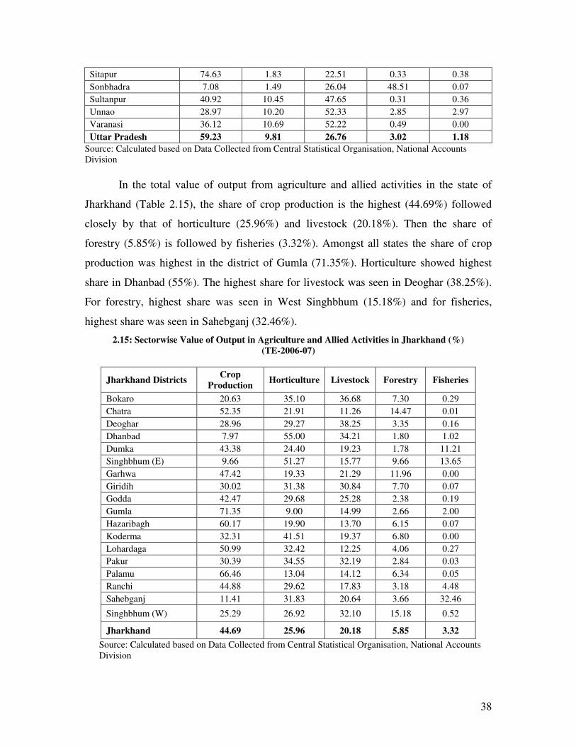
38
Sitapur 74.63 1.83 22.51 0.33 0.38
Sonbhadra 7.08 1.49 26.04 48.51 0.07
Sultanpur 40.92 10.45 47.65 0.31 0.36
Unnao 28.97 10.20 52.33 2.85 2.97
Varanasi 36.12 10.69 52.22 0.49 0.00
Uttar Pradesh 59.23 9.81 26.76 3.02 1.18
Source: Calculated based on Data Collected from Central Statistical Organisation, National Accounts
Division
In the total value of output from agriculture and allied activities in the state of
Jharkhand (Table 2.15), the share of crop production is the highest (44.69%) followed
closely by that of horticulture (25.96%) and livestock (20.18%). Then the share of
forestry (5.85%) is followed by fisheries (3.32%). Amongst all states the share of crop
production was highest in the district of Gumla (71.35%). Horticulture showed highest
share in Dhanbad (55%). The highest share for livestock was seen in Deoghar (38.25%).
For forestry, highest share was seen in West Singhbhum (15.18%) and for fisheries,
highest share was seen in Sahebganj (32.46%).
2.15: Sectorwise Value of Output in Agriculture and Allied Activities in Jharkhand (%)
(TE-2006-07)
Jharkhand Districts Crop
Production Horticulture Livestock Forestry Fisheries
Bokaro 20.63 35.10 36.68 7.30 0.29
Chatra 52.35 21.91 11.26 14.47 0.01
Deoghar 28.96 29.27 38.25 3.35 0.16
Dhanbad 7.97 55.00 34.21 1.80 1.02
Dumka 43.38 24.40 19.23 1.78 11.21
Singhbhum (E) 9.66 51.27 15.77 9.66 13.65
Garhwa 47.42 19.33 21.29 11.96 0.00
Giridih 30.02 31.38 30.84 7.70 0.07
Godda 42.47 29.68 25.28 2.38 0.19
Gumla 71.35 9.00 14.99 2.66 2.00
Hazaribagh 60.17 19.90 13.70 6.15 0.07
Koderma 32.31 41.51 19.37 6.80 0.00
Lohardaga 50.99 32.42 12.25 4.06 0.27
Pakur 30.39 34.55 32.19 2.84 0.03
Palamu 66.46 13.04 14.12 6.34 0.05
Ranchi 44.88 29.62 17.83 3.18 4.48
Sahebganj 11.41 31.83 20.64 3.66 32.46
Singhbhum (W) 25.29 26.92 32.10 15.18 0.52
Jharkhand 44.69 25.96 20.18 5.85 3.32
Source: Calculated based on Data Collected from Central Statistical Organisation, National Accounts
Division

39
In the total value of output from agriculture and allied activities in the state of
West Bengal (Table 2.16), the share of crop production is the highest (36.11%) followed
by that of horticulture (31.19%), livestock (17.38%), fisheries (3.14%) and forestry
(12.18%). Amongst all states the share of crop production was highest in the district of
Malda (66.81%). Horticulture showed highest share in Hoogly (70.23%). The highest
share for livestock was seen in Purulia (37.01%). For forestry, highest share was seen in
Darjeeling (24.09%) and for fisheries, highest share was seen in 24 Parganas (40.92%).
2.16: Sectorwise Value of Output in Agriculture and Allied Activities in West Bengal (%)
(TE-2006-07)
Districts Crop
Production Horticulture Livestock Forestry Fisheries
24 Parganas. 9.16 4.41 24.49 10.92 40.92
Bankura 18.86 29.12 19.79 6.70 3.60
Birbhum 37.96 23.98 25.67 1.03 7.00
Burdwan 40.59 37.28 13.85 0.52 5.01
Cooch-Behar 35.66 29.99 18.64 0.24 14.41
Darjeeling 6.46 12.43 24.06 24.09 1.89
Dinajpur. S 51.92 13.06 21.82 0.11 12.63
Dinajur. N 53.86 21.60 20.49 0.06 3.68
Hooghly 15.33 70.17 7.71 0.01 6.71
Howrah 24.40 35.76 16.93 0.00 22.91
Jalpaiguri 21.99 23.09 14.96 8.94 3.49
Malda 66.23 5.43 17.60 0.13 9.99
Midnapur. E 33.03 6.38 22.35 0.06 38.03
Midnapur. W 31.86 35.17 11.18 3.35 3.10
Murshidabad 59.78 11.86 16.50 0.03 11.71
Nadia 50.19 12.06 24.60 0.07 12.80
Purulia 26.61 2.11 37.01 7.02 13.48
West Bengal 36.11 31.19 17.38 3.14 12.18
Source: Calculated based on Data Collected from Central Statistical Organisation, National Accounts
Division
Horticultural Diversification
From Table 2.17, it is seen that in India, between the years 1991-92 to 2007-08,
the annual compound growth rate of area under fruits was 4.5 percent, while that of its
production was 5.1 percent and productivity growth was 0.6 percent only. In the case of
vegetables, area grew at the annual compound rate of 2.1 percent with production rate of
4.9 percent, while the productivity growth was around 2.7 percent. During this period,
the area under Flowers increased at the annual rate of 8.3 percent and production of
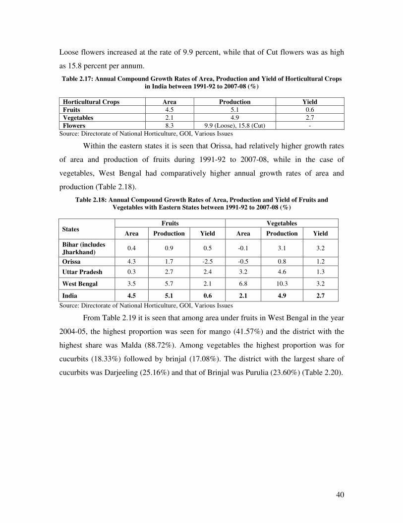
40
Loose flowers increased at the rate of 9.9 percent, while that of Cut flowers was as high
as 15.8 percent per annum.
Table 2.17: Annual Compound Growth Rates of Area, Production and Yield of Horticultural Crops
in India between 1991-92 to 2007-08 (%)
Horticultural Crops Area Production Yield
Fruits 4.5 5.1 0.6
Vegetables 2.1 4.9 2.7
Flowers 8.3 9.9 (Loose), 15.8 (Cut) -
Source: Directorate of National Horticulture, GOI, Various Issues
Within the eastern states it is seen that Orissa, had relatively higher growth rates
of area and production of fruits during 1991-92 to 2007-08, while in the case of
vegetables, West Bengal had comparatively higher annual growth rates of area and
production (Table 2.18).
Table 2.18: Annual Compound Growth Rates of Area, Production and Yield of Fruits and Vegetables with Eastern States between 1991-92 to 2007-08 (%)
States Fruits Vegetables
Area Production Yield Area Production Yield
Bihar (includes Jharkhand)
0.4 0.9 0.5 -0.1 3.1 3.2
Orissa 4.3 1.7 -2.5 -0.5 0.8 1.2
Uttar Pradesh 0.3 2.7 2.4 3.2 4.6 1.3
West Bengal 3.5 5.7 2.1 6.8 10.3 3.2
India 4.5 5.1 0.6 2.1 4.9 2.7
Source: Directorate of National Horticulture, GOI, Various Issues
From Table 2.19 it is seen that among area under fruits in West Bengal in the year
2004-05, the highest proportion was seen for mango (41.57%) and the district with the
highest share was Malda (88.72%). Among vegetables the highest proportion was for
cucurbits (18.33%) followed by brinjal (17.08%). The district with the largest share of
cucurbits was Darjeeling (25.16%) and that of Brinjal was Purulia (23.60%) (Table 2.20).
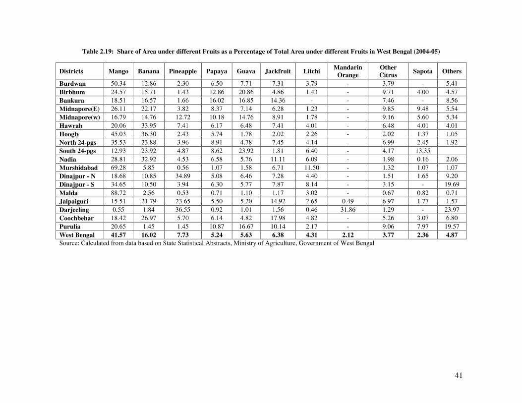
41
Table 2.19: Share of Area under different Fruits as a Percentage of Total Area under different Fruits in West Bengal (2004-05)
Districts Mango Banana Pineapple Papaya Guava Jackfruit Litchi Mandarin
Orange
Other
Citrus Sapota Others
Burdwan 50.34 12.86 2.30 6.50 7.71 7.31 3.79 - 3.79 - 5.41
Birbhum 24.57 15.71 1.43 12.86 20.86 4.86 1.43 - 9.71 4.00 4.57
Bankura 18.51 16.57 1.66 16.02 16.85 14.36 - - 7.46 - 8.56
Midnapore(E) 26.11 22.17 3.82 8.37 7.14 6.28 1.23 - 9.85 9.48 5.54
Midnapore(w) 16.79 14.76 12.72 10.18 14.76 8.91 1.78 - 9.16 5.60 5.34
Hawrah 20.06 33.95 7.41 6.17 6.48 7.41 4.01 - 6.48 4.01 4.01
Hoogly 45.03 36.30 2.43 5.74 1.78 2.02 2.26 - 2.02 1.37 1.05
North 24-pgs 35.53 23.88 3.96 8.91 4.78 7.45 4.14 - 6.99 2.45 1.92
South 24-pgs 12.93 23.92 4.87 8.62 23.92 1.81 6.40 - 4.17 13.35
Nadia 28.81 32.92 4.53 6.58 5.76 11.11 6.09 - 1.98 0.16 2.06
Murshidabad 69.28 5.85 0.56 1.07 1.58 6.71 11.50 - 1.32 1.07 1.07
Dinajpur - N 18.68 10.85 34.89 5.08 6.46 7.28 4.40 - 1.51 1.65 9.20
Dinajpur - S 34.65 10.50 3.94 6.30 5.77 7.87 8.14 - 3.15 - 19.69
Malda 88.72 2.56 0.53 0.71 1.10 1.17 3.02 - 0.67 0.82 0.71
Jalpaiguri 15.51 21.79 23.65 5.50 5.20 14.92 2.65 0.49 6.97 1.77 1.57
Darjeeling 0.55 1.84 36.55 0.92 1.01 1.56 0.46 31.86 1.29 - 23.97
Coochbehar 18.42 26.97 5.70 6.14 4.82 17.98 4.82 - 5.26 3.07 6.80
Purulia 20.65 1.45 1.45 10.87 16.67 10.14 2.17 - 9.06 7.97 19.57
West Bengal 41.57 16.02 7.73 5.24 5.63 6.38 4.31 2.12 3.77 2.36 4.87
Source: Calculated from data based on State Statistical Abstracts, Ministry of Agriculture, Government of West Bengal
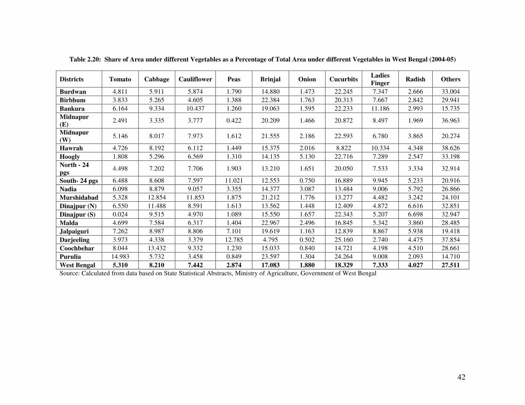
42
Table 2.20: Share of Area under different Vegetables as a Percentage of Total Area under different Vegetables in West Bengal (2004-05)
Districts Tomato Cabbage Cauliflower Peas Brinjal Onion Cucurbits Ladies
Finger Radish Others
Burdwan 4.811 5.911 5.874 1.790 14.880 1.473 22.245 7.347 2.666 33.004
Birbhum 3.833 5.265 4.605 1.388 22.384 1.763 20.313 7.667 2.842 29.941
Bankura 6.164 9.334 10.437 1.260 19.063 1.595 22.233 11.186 2.993 15.735
Midnapur
(E) 2.491 3.335 3.777 0.422 20.209 1.466 20.872 8.497 1.969 36.963
Midnapur (W)
5.146 8.017 7.973 1.612 21.555 2.186 22.593 6.780 3.865 20.274
Hawrah 4.726 8.192 6.112 1.449 15.375 2.016 8.822 10.334 4.348 38.626
Hoogly 1.808 5.296 6.569 1.310 14.135 5.130 22.716 7.289 2.547 33.198
North - 24
pgs 4.498 7.202 7.706 1.903 13.210 1.651 20.050 7.533 3.334 32.914
South- 24 pgs 6.488 8.608 7.597 11.021 12.553 0.750 16.889 9.945 5.233 20.916
Nadia 6.098 8.879 9.057 3.355 14.377 3.087 13.484 9.006 5.792 26.866
Murshidabad 5.328 12.854 11.853 1.875 21.212 1.776 13.277 4.482 3.242 24.101
Dinajpur (N) 6.550 11.488 8.591 1.613 13.562 1.448 12.409 4.872 6.616 32.851
Dinajpur (S) 0.024 9.515 4.970 1.089 15.550 1.657 22.343 5.207 6.698 32.947
Malda 4.699 7.584 6.317 1.404 22.967 2.496 16.845 5.342 3.860 28.485
Jalpaiguri 7.262 8.987 8.806 7.101 19.619 1.163 12.839 8.867 5.938 19.418
Darjeeling 3.973 4.338 3.379 12.785 4.795 0.502 25.160 2.740 4.475 37.854
Coochbehar 8.044 13.432 9.332 1.230 15.033 0.840 14.721 4.198 4.510 28.661
Purulia 14.983 5.732 3.458 0.849 23.597 1.304 24.264 9.008 2.093 14.710
West Bengal 5.310 8.210 7.442 2.874 17.083 1.880 18.329 7.333 4.027 27.511
Source: Calculated from data based on State Statistical Abstracts, Ministry of Agriculture, Government of West Bengal
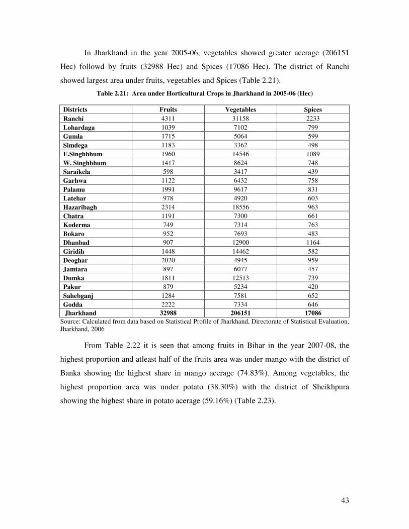
43
In Jharkhand in the year 2005-06, vegetables showed greater acerage (206151
Hec) followd by fruits (32988 Hec) and Spices (17086 Hec). The district of Ranchi
showed largest area under fruits, vegetables and Spices (Table 2.21).
Table 2.21: Area under Horticultural Crops in Jharkhand in 2005-06 (Hec)
Districts Fruits Vegetables Spices
Ranchi 4311 31158 2233
Lohardaga 1039 7102 799
Gumla 1715 5064 599
Simdega 1183 3362 498
E.Singhbhum 1960 14546 1089
W. Singhbhum 1417 8624 748
Saraikela 598 3417 439
Garhwa 1122 6432 758
Palamu 1991 9617 831
Latehar 978 4920 603
Hazaribagh 2314 18556 963
Chatra 1191 7300 661
Koderma 749 7314 763
Bokaro 952 7693 483
Dhanbad 907 12900 1164
Giridih 1448 14462 582
Deoghar 2020 4945 959
Jamtara 897 6077 457
Dumka 1811 12513 739
Pakur 879 5234 420
Sahebganj 1284 7581 652
Godda 2222 7334 646
Jharkhand 32988 206151 17086
Source: Calculated from data based on Statistical Profile of Jharkhand, Directorate of Statistical Evaluation,
Jharkhand, 2006
From Table 2.22 it is seen that among fruits in Bihar in the year 2007-08, the
highest proportion and atleast half of the fruits area was under mango with the district of
Banka showing the highest share in mango acerage (74.83%). Among vegetables, the
highest proportion area was under potato (38.30%) with the district of Sheikhpura
showing the highest share in potato acerage (59.16%) (Table 2.23).
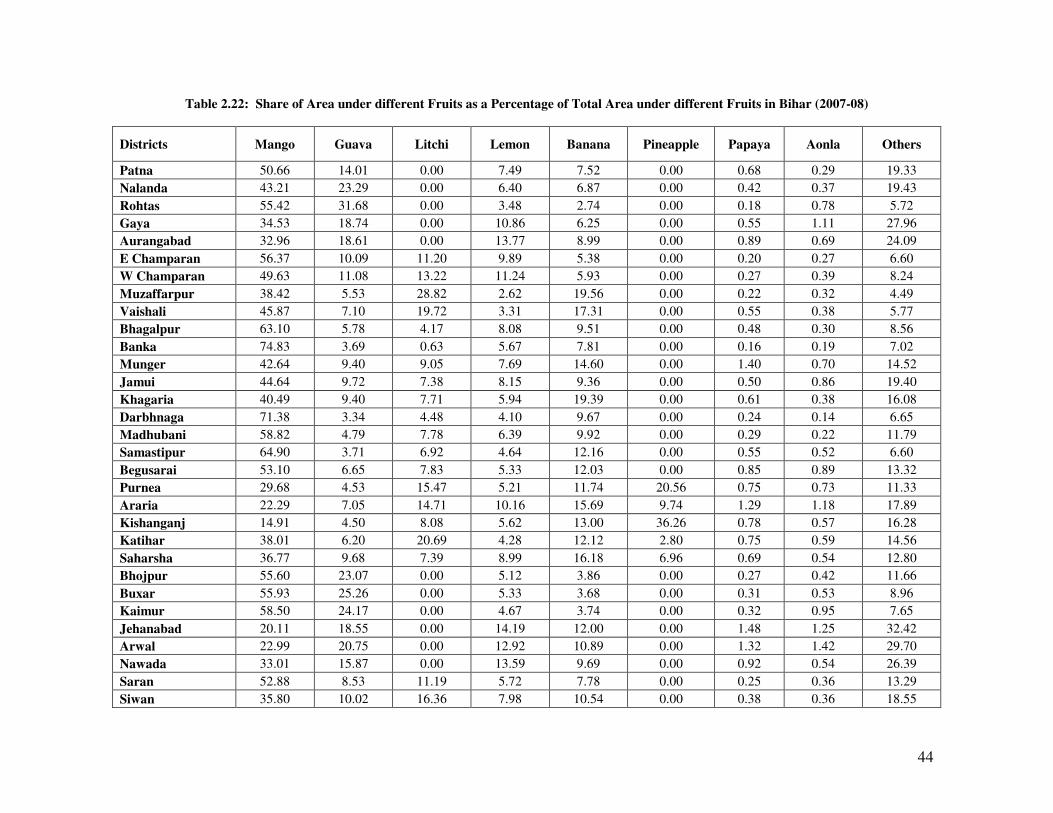
44
Table 2.22: Share of Area under different Fruits as a Percentage of Total Area under different Fruits in Bihar (2007-08)
Districts Mango Guava Litchi Lemon Banana Pineapple Papaya Aonla Others
Patna 50.66 14.01 0.00 7.49 7.52 0.00 0.68 0.29 19.33
Nalanda 43.21 23.29 0.00 6.40 6.87 0.00 0.42 0.37 19.43
Rohtas 55.42 31.68 0.00 3.48 2.74 0.00 0.18 0.78 5.72
Gaya 34.53 18.74 0.00 10.86 6.25 0.00 0.55 1.11 27.96
Aurangabad 32.96 18.61 0.00 13.77 8.99 0.00 0.89 0.69 24.09
E Champaran 56.37 10.09 11.20 9.89 5.38 0.00 0.20 0.27 6.60
W Champaran 49.63 11.08 13.22 11.24 5.93 0.00 0.27 0.39 8.24
Muzaffarpur 38.42 5.53 28.82 2.62 19.56 0.00 0.22 0.32 4.49
Vaishali 45.87 7.10 19.72 3.31 17.31 0.00 0.55 0.38 5.77
Bhagalpur 63.10 5.78 4.17 8.08 9.51 0.00 0.48 0.30 8.56
Banka 74.83 3.69 0.63 5.67 7.81 0.00 0.16 0.19 7.02
Munger 42.64 9.40 9.05 7.69 14.60 0.00 1.40 0.70 14.52
Jamui 44.64 9.72 7.38 8.15 9.36 0.00 0.50 0.86 19.40
Khagaria 40.49 9.40 7.71 5.94 19.39 0.00 0.61 0.38 16.08
Darbhnaga 71.38 3.34 4.48 4.10 9.67 0.00 0.24 0.14 6.65
Madhubani 58.82 4.79 7.78 6.39 9.92 0.00 0.29 0.22 11.79
Samastipur 64.90 3.71 6.92 4.64 12.16 0.00 0.55 0.52 6.60
Begusarai 53.10 6.65 7.83 5.33 12.03 0.00 0.85 0.89 13.32
Purnea 29.68 4.53 15.47 5.21 11.74 20.56 0.75 0.73 11.33
Araria 22.29 7.05 14.71 10.16 15.69 9.74 1.29 1.18 17.89
Kishanganj 14.91 4.50 8.08 5.62 13.00 36.26 0.78 0.57 16.28
Katihar 38.01 6.20 20.69 4.28 12.12 2.80 0.75 0.59 14.56
Saharsha 36.77 9.68 7.39 8.99 16.18 6.96 0.69 0.54 12.80
Bhojpur 55.60 23.07 0.00 5.12 3.86 0.00 0.27 0.42 11.66
Buxar 55.93 25.26 0.00 5.33 3.68 0.00 0.31 0.53 8.96
Kaimur 58.50 24.17 0.00 4.67 3.74 0.00 0.32 0.95 7.65
Jehanabad 20.11 18.55 0.00 14.19 12.00 0.00 1.48 1.25 32.42
Arwal 22.99 20.75 0.00 12.92 10.89 0.00 1.32 1.42 29.70
Nawada 33.01 15.87 0.00 13.59 9.69 0.00 0.92 0.54 26.39
Saran 52.88 8.53 11.19 5.72 7.78 0.00 0.25 0.36 13.29
Siwan 35.80 10.02 16.36 7.98 10.54 0.00 0.38 0.36 18.55
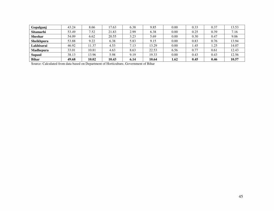
45
Gopalganj 43.24 8.66 17.63 6.38 9.85 0.00 0.33 0.37 13.53
Sitamarhi 53.49 7.52 21.83 2.99 6.38 0.00 0.25 0.39 7.16
Sheohar 54.09 6.62 20.55 3.23 5.69 0.00 0.30 0.47 9.06
Sheikhpura 53.88 9.22 6.38 5.83 9.15 0.00 0.83 0.76 13.94
Lakhisarai 46.92 11.37 4.53 7.13 13.29 0.00 1.45 1.25 14.07
Madhepura 33.01 10.81 4.63 8.63 22.53 6.56 0.77 0.61 12.43
Supaul 38.13 13.96 5.98 9.19 19.33 0.00 0.43 0.43 12.56
Bihar 49.68 10.02 10.43 6.14 10.64 1.62 0.45 0.46 10.57
Source: Calculated from data based on Department of Horticulture, Government of Bihar

46
Table 2.23: Share of Area under different Vegetables as a Percentage of Total Area under different Vegetables in Bihar (2007-08)
Districts Potato Onion Tomato Caulilower Cabbage Brinjal Okra Chilli Bottle
gourd
Sponge
gourd Cucumber
Ridge
gourd
Patna 40.62 6.22 4.62 9.22 5.28 4.65 7.40 6.49 2.29 1.79 0.25 0.70
Nalanda 45.86 9.86 3.16 5.15 2.86 11.00 4.79 6.45 1.47 1.22 0.18 0.54
Bhojpur 44.73 6.14 5.48 5.74 3.69 5.56 8.15 3.24 3.56 2.09 0.42 1.02
Buxar 41.28 7.03 5.93 5.27 3.77 5.27 8.45 3.62 5.21 2.87 0.21 1.20
Rohtas 53.89 5.90 4.11 6.05 3.01 4.91 7.03 3.10 2.42 1.88 0.09 0.75
Kaimur 41.34 8.17 5.57 6.88 3.97 6.52 8.04 3.73 3.69 2.67 0.13 0.90
Gaya 43.73 5.49 3.47 7.36 3.47 6.33 6.82 5.39 4.24 3.39 0.15 1.51
Jehanabad 42.92 5.38 8.53 5.72 3.90 6.92 6.26 4.07 4.82 2.77 0.30 0.96
Arwal 42.03 5.80 6.19 5.93 4.54 5.69 6.46 4.08 5.84 2.81 0.46 1.03
Nawada 35.53 5.87 4.70 8.03 4.47 7.49 11.63 5.16 4.27 3.89 0.17 1.04
Aurangabad 34.92 6.35 9.13 7.85 4.15 6.51 10.52 4.07 3.79 3.01 0.11 0.74
Saran 47.02 3.23 5.55 7.23 3.43 6.28 7.01 4.01 3.23 3.04 0.12 0.74
Siwan 44.62 3.72 5.88 6.87 3.72 6.84 8.73 4.55 3.51 3.18 0.08 0.66
Gopalganj 46.74 3.28 5.75 7.19 3.98 5.33 8.42 3.90 4.32 2.55 0.09 0.72
E.Champaran 37.14 7.46 5.62 6.37 4.93 5.42 8.45 3.59 4.38 4.64 0.12 0.87
W.Champaran 35.96 6.74 5.80 8.41 4.61 5.74 7.83 4.24 4.39 4.35 0.11 0.87
Muzaffarpur 29.34 6.18 8.83 9.27 6.76 6.96 6.57 4.51 4.23 4.78 0.25 0.93
Sitamarhi 35.94 6.84 7.90 6.87 4.95 6.45 5.67 3.83 5.62 4.83 0.11 0.93
Sheohar 39.09 6.35 4.94 7.57 5.95 5.92 5.46 3.97 5.01 4.15 0.17 0.96
Vaishali 30.56 3.84 8.70 11.14 5.40 6.93 7.93 3.73 3.71 4.61 0.26 0.98
Bhagalpur 34.44 6.41 6.64 6.10 4.78 6.50 8.47 3.84 4.58 4.86 0.34 1.42
Banka 50.00 5.55 4.66 5.29 3.18 6.22 7.04 3.97 3.06 3.21 0.14 0.87
Munger 45.16 6.12 4.21 4.48 3.17 4.46 6.31 7.04 3.12 3.24 0.44 1.01
Sheikhpura 59.16 10.90 2.36 2.18 2.03 3.06 3.19 7.04 2.67 2.03 0.16 0.89
Lakhisarai 50.72 4.75 3.61 3.83 3.16 2.93 4.51 6.18 4.17 3.16 0.60 1.29
Jamui 38.95 8.04 4.40 4.41 4.14 6.12 7.49 9.50 3.62 4.29 0.18 1.18
Khagaria 33.24 4.57 6.64 7.36 4.09 8.55 9.11 5.81 3.05 4.52 0.14 2.09
Darbhanga 29.27 4.07 5.59 6.02 6.21 9.19 6.33 5.20 4.15 7.85 0.11 1.14
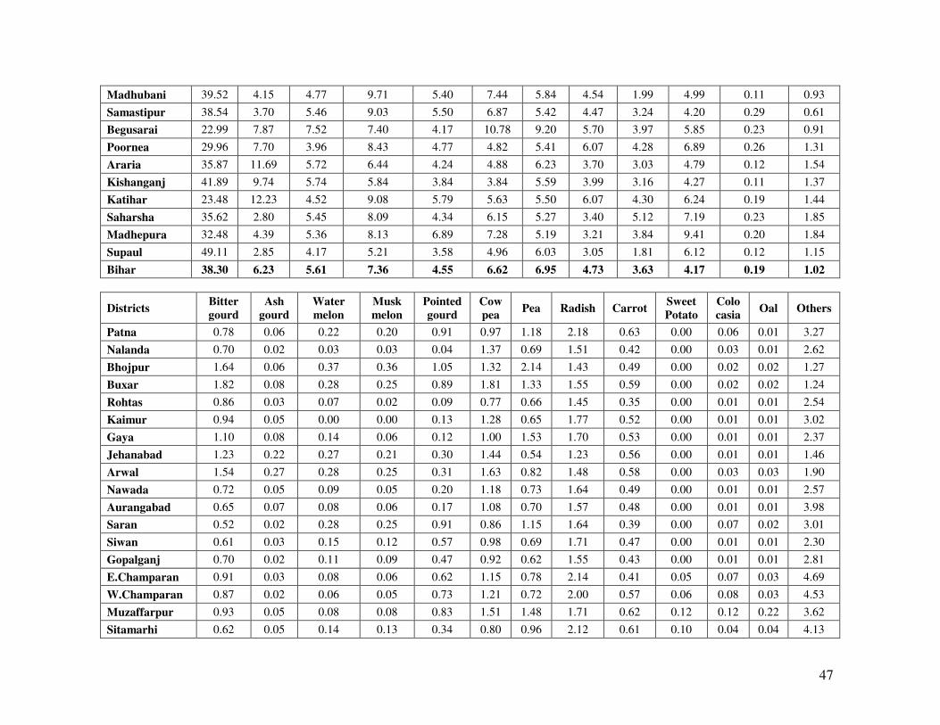
47
Madhubani 39.52 4.15 4.77 9.71 5.40 7.44 5.84 4.54 1.99 4.99 0.11 0.93
Samastipur 38.54 3.70 5.46 9.03 5.50 6.87 5.42 4.47 3.24 4.20 0.29 0.61
Begusarai 22.99 7.87 7.52 7.40 4.17 10.78 9.20 5.70 3.97 5.85 0.23 0.91
Poornea 29.96 7.70 3.96 8.43 4.77 4.82 5.41 6.07 4.28 6.89 0.26 1.31
Araria 35.87 11.69 5.72 6.44 4.24 4.88 6.23 3.70 3.03 4.79 0.12 1.54
Kishanganj 41.89 9.74 5.74 5.84 3.84 3.84 5.59 3.99 3.16 4.27 0.11 1.37
Katihar 23.48 12.23 4.52 9.08 5.79 5.63 5.50 6.07 4.30 6.24 0.19 1.44
Saharsha 35.62 2.80 5.45 8.09 4.34 6.15 5.27 3.40 5.12 7.19 0.23 1.85
Madhepura 32.48 4.39 5.36 8.13 6.89 7.28 5.19 3.21 3.84 9.41 0.20 1.84
Supaul 49.11 2.85 4.17 5.21 3.58 4.96 6.03 3.05 1.81 6.12 0.12 1.15
Bihar 38.30 6.23 5.61 7.36 4.55 6.62 6.95 4.73 3.63 4.17 0.19 1.02
Districts Bitter gourd
Ash gourd
Water melon
Musk melon
Pointed gourd
Cow pea
Pea Radish Carrot Sweet Potato
Colo casia
Oal Others
Patna 0.78 0.06 0.22 0.20 0.91 0.97 1.18 2.18 0.63 0.00 0.06 0.01 3.27
Nalanda 0.70 0.02 0.03 0.03 0.04 1.37 0.69 1.51 0.42 0.00 0.03 0.01 2.62
Bhojpur 1.64 0.06 0.37 0.36 1.05 1.32 2.14 1.43 0.49 0.00 0.02 0.02 1.27
Buxar 1.82 0.08 0.28 0.25 0.89 1.81 1.33 1.55 0.59 0.00 0.02 0.02 1.24
Rohtas 0.86 0.03 0.07 0.02 0.09 0.77 0.66 1.45 0.35 0.00 0.01 0.01 2.54
Kaimur 0.94 0.05 0.00 0.00 0.13 1.28 0.65 1.77 0.52 0.00 0.01 0.01 3.02
Gaya 1.10 0.08 0.14 0.06 0.12 1.00 1.53 1.70 0.53 0.00 0.01 0.01 2.37
Jehanabad 1.23 0.22 0.27 0.21 0.30 1.44 0.54 1.23 0.56 0.00 0.01 0.01 1.46
Arwal 1.54 0.27 0.28 0.25 0.31 1.63 0.82 1.48 0.58 0.00 0.03 0.03 1.90
Nawada 0.72 0.05 0.09 0.05 0.20 1.18 0.73 1.64 0.49 0.00 0.01 0.01 2.57
Aurangabad 0.65 0.07 0.08 0.06 0.17 1.08 0.70 1.57 0.48 0.00 0.01 0.01 3.98
Saran 0.52 0.02 0.28 0.25 0.91 0.86 1.15 1.64 0.39 0.00 0.07 0.02 3.01
Siwan 0.61 0.03 0.15 0.12 0.57 0.98 0.69 1.71 0.47 0.00 0.01 0.01 2.30
Gopalganj 0.70 0.02 0.11 0.09 0.47 0.92 0.62 1.55 0.43 0.00 0.01 0.01 2.81
E.Champaran 0.91 0.03 0.08 0.06 0.62 1.15 0.78 2.14 0.41 0.05 0.07 0.03 4.69
W.Champaran 0.87 0.02 0.06 0.05 0.73 1.21 0.72 2.00 0.57 0.06 0.08 0.03 4.53
Muzaffarpur 0.93 0.05 0.08 0.08 0.83 1.51 1.48 1.71 0.62 0.12 0.12 0.22 3.62
Sitamarhi 0.62 0.05 0.14 0.13 0.34 0.80 0.96 2.12 0.61 0.10 0.04 0.04 4.13
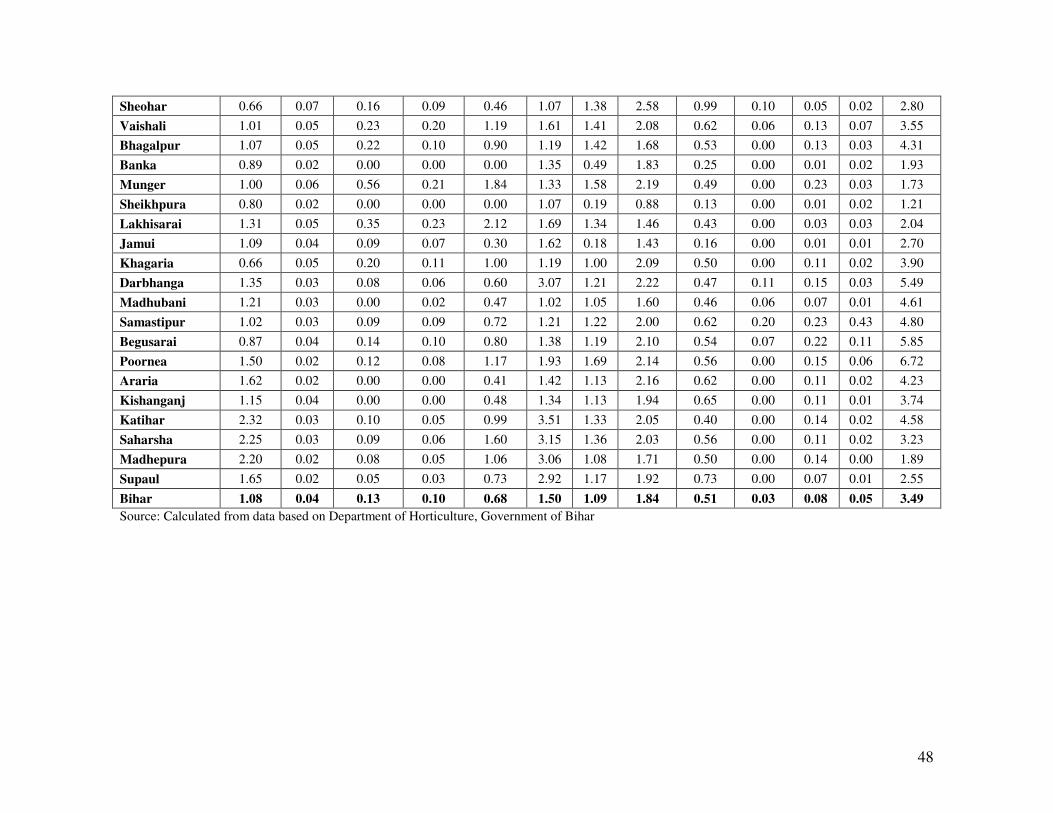
48
Sheohar 0.66 0.07 0.16 0.09 0.46 1.07 1.38 2.58 0.99 0.10 0.05 0.02 2.80
Vaishali 1.01 0.05 0.23 0.20 1.19 1.61 1.41 2.08 0.62 0.06 0.13 0.07 3.55
Bhagalpur 1.07 0.05 0.22 0.10 0.90 1.19 1.42 1.68 0.53 0.00 0.13 0.03 4.31
Banka 0.89 0.02 0.00 0.00 0.00 1.35 0.49 1.83 0.25 0.00 0.01 0.02 1.93
Munger 1.00 0.06 0.56 0.21 1.84 1.33 1.58 2.19 0.49 0.00 0.23 0.03 1.73
Sheikhpura 0.80 0.02 0.00 0.00 0.00 1.07 0.19 0.88 0.13 0.00 0.01 0.02 1.21
Lakhisarai 1.31 0.05 0.35 0.23 2.12 1.69 1.34 1.46 0.43 0.00 0.03 0.03 2.04
Jamui 1.09 0.04 0.09 0.07 0.30 1.62 0.18 1.43 0.16 0.00 0.01 0.01 2.70
Khagaria 0.66 0.05 0.20 0.11 1.00 1.19 1.00 2.09 0.50 0.00 0.11 0.02 3.90
Darbhanga 1.35 0.03 0.08 0.06 0.60 3.07 1.21 2.22 0.47 0.11 0.15 0.03 5.49
Madhubani 1.21 0.03 0.00 0.02 0.47 1.02 1.05 1.60 0.46 0.06 0.07 0.01 4.61
Samastipur 1.02 0.03 0.09 0.09 0.72 1.21 1.22 2.00 0.62 0.20 0.23 0.43 4.80
Begusarai 0.87 0.04 0.14 0.10 0.80 1.38 1.19 2.10 0.54 0.07 0.22 0.11 5.85
Poornea 1.50 0.02 0.12 0.08 1.17 1.93 1.69 2.14 0.56 0.00 0.15 0.06 6.72
Araria 1.62 0.02 0.00 0.00 0.41 1.42 1.13 2.16 0.62 0.00 0.11 0.02 4.23
Kishanganj 1.15 0.04 0.00 0.00 0.48 1.34 1.13 1.94 0.65 0.00 0.11 0.01 3.74
Katihar 2.32 0.03 0.10 0.05 0.99 3.51 1.33 2.05 0.40 0.00 0.14 0.02 4.58
Saharsha 2.25 0.03 0.09 0.06 1.60 3.15 1.36 2.03 0.56 0.00 0.11 0.02 3.23
Madhepura 2.20 0.02 0.08 0.05 1.06 3.06 1.08 1.71 0.50 0.00 0.14 0.00 1.89
Supaul 1.65 0.02 0.05 0.03 0.73 2.92 1.17 1.92 0.73 0.00 0.07 0.01 2.55
Bihar 1.08 0.04 0.13 0.10 0.68 1.50 1.09 1.84 0.51 0.03 0.08 0.05 3.49
Source: Calculated from data based on Department of Horticulture, Government of Bihar
49
From Table 2.24 it is seen that among area under fruits in Uttar Pradesh in the
year 2007-08, the highest proportion was seen for mango (85.53%) with the district of
Balrampur showing 100% acerage under the fruit. Among vegetables the highest
proportion was for potato (47.72%) and the district with the largest share of the vegetable
was Mathura (91.04%) (Table 2.25).
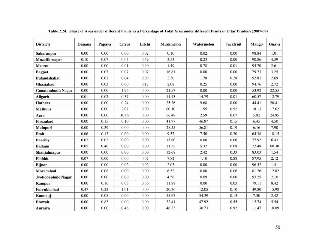
50
Table 2.24: Share of Area under different Fruits as a Percentage of Total Area under different Fruits in Uttar Pradesh (2007-08)
Districts Banana Papaya Citrus Litchi Muskmelon Watermelon Jackfruit Mango Guava
Saharanpur 0.00 0.00 0.00 0.02 0.10 0.02 0.00 98.84 1.01
Muzaffarnagar 0.10 0.07 0.04 0.59 3.53 0.23 0.00 90.86 4.59
Meerut 0.00 0.00 0.01 0.40 1.49 0.78 0.01 94.70 2.61
Bagpat 0.00 0.07 0.07 0.07 16.81 0.00 0.00 79.73 3.25
Bulandshahar 0.00 0.01 0.04 0.09 2.30 1.78 0.28 92.81 2.69
Ghaziabad 0.00 0.03 0.00 0.17 2.08 0.25 0.00 94.76 2.72
Gauatambudh Nagar 0.00 0.00 1.96 0.00 21.57 0.00 0.00 53.92 22.55
Aligarh 0.01 0.02 0.37 0.00 11.43 14.79 0.01 60.57 12.79
Hathras 0.00 0.00 0.24 0.00 25.26 9.68 0.00 44.41 20.41
Mathura 0.00 0.00 2.07 0.00 60.10 1.55 0.52 18.13 17.62
Agra 0.00 0.00 10.09 0.00 56.48 2.59 0.07 5.82 24.95
Firozabad 0.00 0.15 0.10 0.00 41.77 46.87 0.15 6.45 4.50
Mainpuri 0.00 0.39 0.00 0.00 28.55 56.81 0.19 6.16 7.90
Etah 0.06 0.13 0.00 0.00 9.57 7.50 0.20 64.38 18.15
Bareilly 0.02 0.02 0.00 0.00 15.60 0.00 0.00 77.92 6.43
Badaun 0.05 0.46 0.00 0.00 11.32 5.32 0.08 22.48 60.30
Shahjahnapur 0.00 0.00 0.00 0.00 12.68 2.42 0.33 83.03 1.54
Pilibhit 0.07 0.00 0.00 0.07 7.82 1.10 0.88 87.95 2.12
Bijnor 0.00 0.00 0.02 0.02 2.03 0.00 0.00 96.52 1.41
Moradabad 0.06 0.08 0.00 0.00 6.52 0.00 0.06 81.26 12.02
Jyotiobaphule Nagar 0.00 0.00 0.00 0.00 4.56 0.09 0.00 93.25 2.10
Rampur 0.00 0.16 0.03 0.36 11.88 0.00 0.03 79.11 8.42
Farrukhabad 0.47 0.23 1.01 0.00 20.36 12.05 0.10 49.80 15.98
Kannauj 0.00 0.08 0.00 0.00 55.67 34.39 0.13 7.30 2.42
Etawah 0.00 0.83 0.00 0.00 32.41 47.92 0.55 12.74 5.54
Auraiya 0.00 0.00 0.46 0.00 46.33 30.73 0.92 11.47 10.09
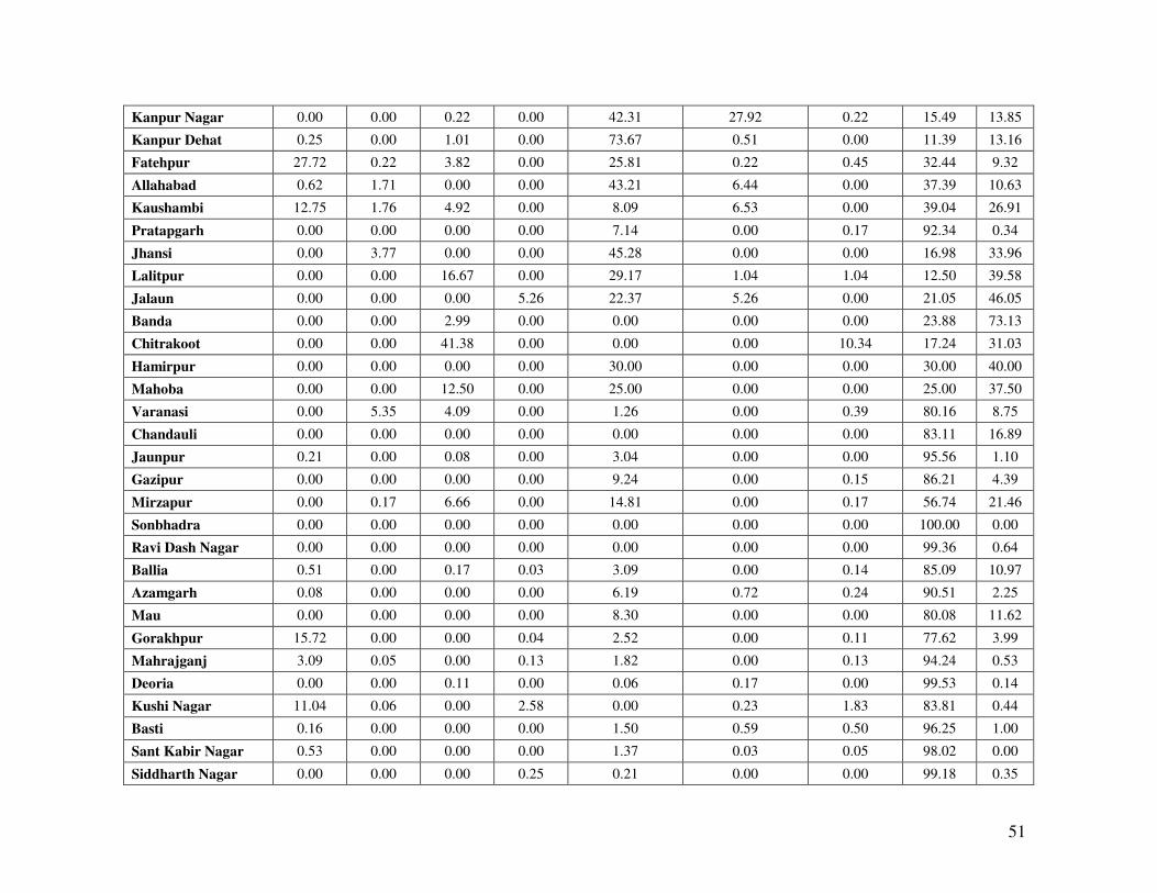
51
Kanpur Nagar 0.00 0.00 0.22 0.00 42.31 27.92 0.22 15.49 13.85
Kanpur Dehat 0.25 0.00 1.01 0.00 73.67 0.51 0.00 11.39 13.16
Fatehpur 27.72 0.22 3.82 0.00 25.81 0.22 0.45 32.44 9.32
Allahabad 0.62 1.71 0.00 0.00 43.21 6.44 0.00 37.39 10.63
Kaushambi 12.75 1.76 4.92 0.00 8.09 6.53 0.00 39.04 26.91
Pratapgarh 0.00 0.00 0.00 0.00 7.14 0.00 0.17 92.34 0.34
Jhansi 0.00 3.77 0.00 0.00 45.28 0.00 0.00 16.98 33.96
Lalitpur 0.00 0.00 16.67 0.00 29.17 1.04 1.04 12.50 39.58
Jalaun 0.00 0.00 0.00 5.26 22.37 5.26 0.00 21.05 46.05
Banda 0.00 0.00 2.99 0.00 0.00 0.00 0.00 23.88 73.13
Chitrakoot 0.00 0.00 41.38 0.00 0.00 0.00 10.34 17.24 31.03
Hamirpur 0.00 0.00 0.00 0.00 30.00 0.00 0.00 30.00 40.00
Mahoba 0.00 0.00 12.50 0.00 25.00 0.00 0.00 25.00 37.50
Varanasi 0.00 5.35 4.09 0.00 1.26 0.00 0.39 80.16 8.75
Chandauli 0.00 0.00 0.00 0.00 0.00 0.00 0.00 83.11 16.89
Jaunpur 0.21 0.00 0.08 0.00 3.04 0.00 0.00 95.56 1.10
Gazipur 0.00 0.00 0.00 0.00 9.24 0.00 0.15 86.21 4.39
Mirzapur 0.00 0.17 6.66 0.00 14.81 0.00 0.17 56.74 21.46
Sonbhadra 0.00 0.00 0.00 0.00 0.00 0.00 0.00 100.00 0.00
Ravi Dash Nagar 0.00 0.00 0.00 0.00 0.00 0.00 0.00 99.36 0.64
Ballia 0.51 0.00 0.17 0.03 3.09 0.00 0.14 85.09 10.97
Azamgarh 0.08 0.00 0.00 0.00 6.19 0.72 0.24 90.51 2.25
Mau 0.00 0.00 0.00 0.00 8.30 0.00 0.00 80.08 11.62
Gorakhpur 15.72 0.00 0.00 0.04 2.52 0.00 0.11 77.62 3.99
Mahrajganj 3.09 0.05 0.00 0.13 1.82 0.00 0.13 94.24 0.53
Deoria 0.00 0.00 0.11 0.00 0.06 0.17 0.00 99.53 0.14
Kushi Nagar 11.04 0.06 0.00 2.58 0.00 0.23 1.83 83.81 0.44
Basti 0.16 0.00 0.00 0.00 1.50 0.59 0.50 96.25 1.00
Sant Kabir Nagar 0.53 0.00 0.00 0.00 1.37 0.03 0.05 98.02 0.00
Siddharth Nagar 0.00 0.00 0.00 0.25 0.21 0.00 0.00 99.18 0.35
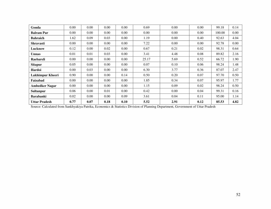
52
Gonda 0.00 0.00 0.00 0.00 0.69 0.00 0.00 99.18 0.14
Balram Pur 0.00 0.00 0.00 0.00 0.00 0.00 0.00 100.00 0.00
Bahraich 1.62 0.09 0.03 0.00 1.19 0.00 0.40 92.63 4.04
Shravasti 0.00 0.00 0.00 0.00 7.22 0.00 0.00 92.78 0.00
Lucknow 0.12 0.00 0.02 0.00 0.67 0.21 0.02 98.31 0.64
Unnao 0.01 0.01 0.03 0.00 3.41 4.48 0.08 89.82 2.16
Raebareli 0.00 0.00 0.00 0.00 25.17 5.69 0.52 66.72 1.90
Sitapur 0.05 0.00 0.00 0.00 0.07 0.10 0.06 98.24 1.48
Hardoi 0.00 0.03 0.00 0.00 6.30 3.77 0.36 87.07 2.47
Lakhimpur Kheeri 0.90 0.00 0.00 0.14 0.50 0.20 0.07 97.70 0.50
Faizabad 0.00 0.00 0.00 0.00 1.85 0.34 0.07 95.97 1.77
Ambedker Nagar 0.00 0.00 0.00 0.00 1.15 0.09 0.02 98.24 0.50
Sultanpur 0.06 0.00 0.01 0.00 0.42 0.00 0.04 99.31 0.16
Barabanki 0.02 0.00 0.00 0.09 3.61 0.04 0.11 95.00 1.14
Uttar Pradesh 0.77 0.07 0.18 0.10 5.52 2.91 0.12 85.53 4.82
Source: Calculated from Sankhyakiya Patrika, Economics & Statistics Division of Planning Department, Government of Uttar Pradesh
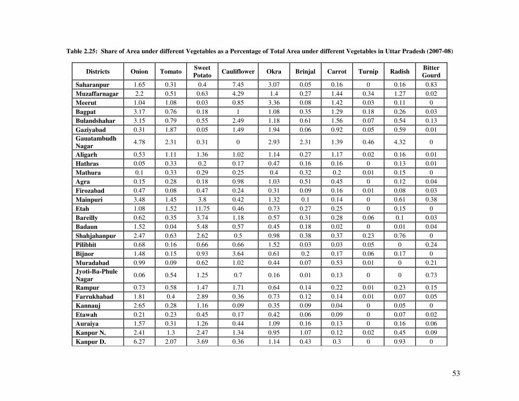
53
Table 2.25: Share of Area under different Vegetables as a Percentage of Total Area under different Vegetables in Uttar Pradesh (2007-08)
Districts Onion Tomato Sweet
Potato Cauliflower Okra Brinjal Carrot Turnip Radish
Bitter
Gourd
Saharanpur 1.65 0.31 0.4 7.45 3.07 0.05 0.16 0 0.16 0.83
Muzaffarnagar 2.2 0.51 0.63 4.29 1.4 0.27 1.44 0.34 1.27 0.02
Meerut 1.04 1.08 0.03 0.85 3.36 0.08 1.42 0.03 0.11 0
Bagpat 3.17 0.76 0.18 1 1.08 0.35 1.29 0.18 0.26 0.03
Bulandshahar 3.15 0.79 0.55 2.49 1.18 0.61 1.56 0.07 0.54 0.13
Gaziyabad 0.31 1.87 0.05 1.49 1.94 0.06 0.92 0.05 0.59 0.01
Gauatambudh
Nagar 4.78 2.31 0.31 0 2.93 2.31 1.39 0.46 4.32 0
Aligarh 0.53 1.11 1.36 1.02 1.14 0.27 1.17 0.02 0.16 0.01
Hathras 0.05 0.33 0.2 0.17 0.47 0.16 0.16 0 0.13 0.01
Mathura 0.1 0.33 0.29 0.25 0.4 0.32 0.2 0.01 0.15 0
Agra 0.15 0.28 0.18 0.98 1.03 0.51 0.45 0 0.12 0.04
Firozabad 0.47 0.08 0.47 0.24 0.31 0.09 0.16 0.01 0.08 0.03
Mainpuri 3.48 1.45 3.8 0.42 1.32 0.1 0.14 0 0.61 0.38
Etah 1.08 1.52 11.75 0.46 0.73 0.27 0.25 0 0.15 0
Bareilly 0.62 0.35 3.74 1.18 0.57 0.31 0.28 0.06 0.1 0.03
Badaun 1.52 0.04 5.48 0.57 0.45 0.18 0.02 0 0.01 0.04
Shahjahanpur 2.47 0.63 2.62 0.5 0.98 0.38 0.37 0.23 0.76 0
Pilibhit 0.68 0.16 0.66 0.66 1.52 0.03 0.03 0.05 0 0.24
Bijnor 1.48 0.15 0.93 3.64 0.61 0.2 0.17 0.06 0.17 0
Muradabad 0.99 0.09 0.62 1.02 0.44 0.07 0.53 0.01 0 0.21
Jyoti-Ba-Phule
Nagar 0.06 0.54 1.25 0.7 0.16 0.01 0.13 0 0 0.73
Rampur 0.73 0.58 1.47 1.71 0.64 0.14 0.22 0.01 0.23 0.15
Farrukhabad 1.81 0.4 2.89 0.36 0.73 0.12 0.14 0.01 0.07 0.05
Kannauj 2.65 0.28 1.16 0.09 0.35 0.09 0.04 0 0.05 0
Etawah 0.21 0.23 0.45 0.17 0.42 0.06 0.09 0 0.07 0.02
Auraiya 1.57 0.31 1.26 0.44 1.09 0.16 0.13 0 0.16 0.06
Kanpur N. 2.41 1.3 2.47 1.34 0.95 1.07 0.12 0.02 0.45 0.09
Kanpur D. 6.27 2.07 3.69 0.36 1.14 0.43 0.3 0 0.93 0
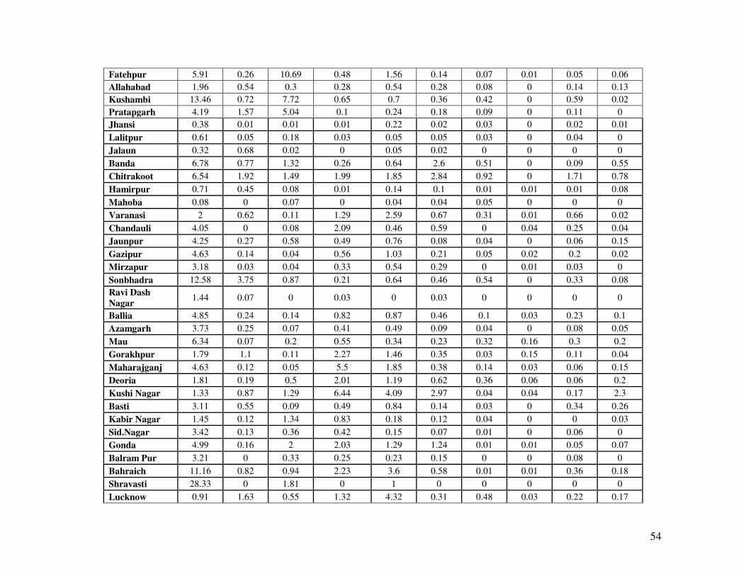
54
Fatehpur 5.91 0.26 10.69 0.48 1.56 0.14 0.07 0.01 0.05 0.06
Allahabad 1.96 0.54 0.3 0.28 0.54 0.28 0.08 0 0.14 0.13
Kushambi 13.46 0.72 7.72 0.65 0.7 0.36 0.42 0 0.59 0.02
Pratapgarh 4.19 1.57 5.04 0.1 0.24 0.18 0.09 0 0.11 0
Jhansi 0.38 0.01 0.01 0.01 0.22 0.02 0.03 0 0.02 0.01
Lalitpur 0.61 0.05 0.18 0.03 0.05 0.05 0.03 0 0.04 0
Jalaun 0.32 0.68 0.02 0 0.05 0.02 0 0 0 0
Banda 6.78 0.77 1.32 0.26 0.64 2.6 0.51 0 0.09 0.55
Chitrakoot 6.54 1.92 1.49 1.99 1.85 2.84 0.92 0 1.71 0.78
Hamirpur 0.71 0.45 0.08 0.01 0.14 0.1 0.01 0.01 0.01 0.08
Mahoba 0.08 0 0.07 0 0.04 0.04 0.05 0 0 0
Varanasi 2 0.62 0.11 1.29 2.59 0.67 0.31 0.01 0.66 0.02
Chandauli 4.05 0 0.08 2.09 0.46 0.59 0 0.04 0.25 0.04
Jaunpur 4.25 0.27 0.58 0.49 0.76 0.08 0.04 0 0.06 0.15
Gazipur 4.63 0.14 0.04 0.56 1.03 0.21 0.05 0.02 0.2 0.02
Mirzapur 3.18 0.03 0.04 0.33 0.54 0.29 0 0.01 0.03 0
Sonbhadra 12.58 3.75 0.87 0.21 0.64 0.46 0.54 0 0.33 0.08
Ravi Dash
Nagar 1.44 0.07 0 0.03 0 0.03 0 0 0 0
Ballia 4.85 0.24 0.14 0.82 0.87 0.46 0.1 0.03 0.23 0.1
Azamgarh 3.73 0.25 0.07 0.41 0.49 0.09 0.04 0 0.08 0.05
Mau 6.34 0.07 0.2 0.55 0.34 0.23 0.32 0.16 0.3 0.2
Gorakhpur 1.79 1.1 0.11 2.27 1.46 0.35 0.03 0.15 0.11 0.04
Maharajganj 4.63 0.12 0.05 5.5 1.85 0.38 0.14 0.03 0.06 0.15
Deoria 1.81 0.19 0.5 2.01 1.19 0.62 0.36 0.06 0.06 0.2
Kushi Nagar 1.33 0.87 1.29 6.44 4.09 2.97 0.04 0.04 0.17 2.3
Basti 3.11 0.55 0.09 0.49 0.84 0.14 0.03 0 0.34 0.26
Kabir Nagar 1.45 0.12 1.34 0.83 0.18 0.12 0.04 0 0 0.03
Sid.Nagar 3.42 0.13 0.36 0.42 0.15 0.07 0.01 0 0.06 0
Gonda 4.99 0.16 2 2.03 1.29 1.24 0.01 0.01 0.05 0.07
Balram Pur 3.21 0 0.33 0.25 0.23 0.15 0 0 0.08 0
Bahraich 11.16 0.82 0.94 2.23 3.6 0.58 0.01 0.01 0.36 0.18
Shravasti 28.33 0 1.81 0 1 0 0 0 0 0
Lucknow 0.91 1.63 0.55 1.32 4.32 0.31 0.48 0.03 0.22 0.17
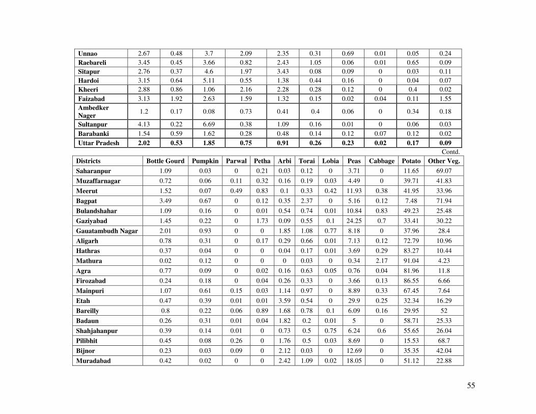
55
Unnao 2.67 0.48 3.7 2.09 2.35 0.31 0.69 0.01 0.05 0.24
Raebareli 3.45 0.45 3.66 0.82 2.43 1.05 0.06 0.01 0.65 0.09
Sitapur 2.76 0.37 4.6 1.97 3.43 0.08 0.09 0 0.03 0.11
Hardoi 3.15 0.64 5.11 0.55 1.38 0.44 0.16 0 0.04 0.07
Kheeri 2.88 0.86 1.06 2.16 2.28 0.28 0.12 0 0.4 0.02
Faizabad 3.13 1.92 2.63 1.59 1.32 0.15 0.02 0.04 0.11 1.55
Ambedker
Nager 1.2 0.17 0.08 0.73 0.41 0.4 0.06 0 0.34 0.18
Sultanpur 4.13 0.22 6.69 0.38 1.09 0.16 0.01 0 0.06 0.03
Barabanki 1.54 0.59 1.62 0.28 0.48 0.14 0.12 0.07 0.12 0.02
Uttar Pradesh 2.02 0.53 1.85 0.75 0.91 0.26 0.23 0.02 0.17 0.09
Contd.
Districts Bottle Gourd Pumpkin Parwal Petha Arbi Torai Lobia Peas Cabbage Potato Other Veg.
Saharanpur 1.09 0.03 0 0.21 0.03 0.12 0 3.71 0 11.65 69.07
Muzaffarnagar 0.72 0.06 0.11 0.32 0.16 0.19 0.03 4.49 0 39.71 41.83
Meerut 1.52 0.07 0.49 0.83 0.1 0.33 0.42 11.93 0.38 41.95 33.96
Bagpat 3.49 0.67 0 0.12 0.35 2.37 0 5.16 0.12 7.48 71.94
Bulandshahar 1.09 0.16 0 0.01 0.54 0.74 0.01 10.84 0.83 49.23 25.48
Gaziyabad 1.45 0.22 0 1.73 0.09 0.55 0.1 24.25 0.7 33.41 30.22
Gauatambudh Nagar 2.01 0.93 0 0 1.85 1.08 0.77 8.18 0 37.96 28.4
Aligarh 0.78 0.31 0 0.17 0.29 0.66 0.01 7.13 0.12 72.79 10.96
Hathras 0.37 0.04 0 0 0.04 0.17 0.01 3.69 0.29 83.27 10.44
Mathura 0.02 0.12 0 0 0 0.03 0 0.34 2.17 91.04 4.23
Agra 0.77 0.09 0 0.02 0.16 0.63 0.05 0.76 0.04 81.96 11.8
Firozabad 0.24 0.18 0 0.04 0.26 0.33 0 3.66 0.13 86.55 6.66
Mainpuri 1.07 0.61 0.15 0.03 1.14 0.97 0 8.89 0.33 67.45 7.64
Etah 0.47 0.39 0.01 0.01 3.59 0.54 0 29.9 0.25 32.34 16.29
Bareilly 0.8 0.22 0.06 0.89 1.68 0.78 0.1 6.09 0.16 29.95 52
Badaun 0.26 0.31 0.01 0.04 1.82 0.2 0.01 5 0 58.71 25.33
Shahjahanpur 0.39 0.14 0.01 0 0.73 0.5 0.75 6.24 0.6 55.65 26.04
Pilibhit 0.45 0.08 0.26 0 1.76 0.5 0.03 8.69 0 15.53 68.7
Bijnor 0.23 0.03 0.09 0 2.12 0.03 0 12.69 0 35.35 42.04
Muradabad 0.42 0.02 0 0 2.42 1.09 0.02 18.05 0 51.12 22.88

56
Jyoti-Ba-Phule Nagar 1.55 0 0 0 7.78 0.69 1.85 2.46 0 57.71 24.37
Rampur 0.55 0.14 0.03 0 0.55 0.56 0 10.51 0 30.57 51.21
Farrukhabad 0.19 0.35 0.01 0 0.78 0.28 0 1.47 0.08 82.83 7.43
Kannauj 0.08 0.68 0 0 0.18 0.09 0.01 2.03 0.01 85.29 6.92
Etawah 0.43 0.29 0.03 0.01 1.97 0.42 0 14.28 0.04 66.09 14.72
Auraiya 0.86 0.43 0 0.01 0.86 1.11 0.03 10.52 0.15 65.41 15.43
Kanpur N. 0.46 0.46 0 0 0.6 0.61 0.18 9.71 0.33 60 17.43
Kanpur D. 0.56 0.38 0 0 0.02 0.55 0.01 31.31 0.01 36.4 15.55
Fatehpur 0.38 0.41 0.14 0.01 0.9 0.54 0.07 12.89 0.01 32.89 32.54
Allahabad 0.2 0.71 0.2 0.03 0.01 0.05 0 12.68 0.06 59.05 22.74
Kushambi 0.01 0.15 0 0.15 0.48 0.01 0.01 20.21 0.1 52.75 1.47
Pratapgarh 0.02 0.03 0.01 0 0 0 0 31.77 0.03 46.75 9.88
Jhansi 0.03 0.01 0 0 0.07 0 0.01 90.43 0 1.92 6.8
Lalitpur 0.01 0 0 0 0.01 0 0.01 91.28 0 1.57 6.08
Jalaun 0.07 0.01 0 0 0.01 0.05 0 92.28 0.01 0.85 5.64
Banda 0.43 0.34 0 0 0 0.34 0.04 31.23 0 1.79 52.3
Chitrakoot 1.49 0.92 0 0 0.14 0.43 0 18.28 0.5 3.98 54.2
Hamirpur 0.05 0.06 0 0 0.01 0.05 0.05 87.8 0.01 1.41 8.98
Mahoba 0 0 0 0 0 0 0 93.8 0 1.38 4.54
Varanasi 0.15 0.24 0.03 0.21 0.01 0.11 0.02 30.55 0.13 34.73 25.54
Chandauli 0.13 0 0 0 0 0 0 16.34 0.25 45.3 30.38
Jaunpur 0.13 0.1 0 0.03 0.02 0.02 0 35.42 0.1 50.77 6.72
Gazipur 0.38 0.02 1.08 0.57 0.02 0.05 0 23.66 0.02 50.53 16.78
Mirzapur 0 0 0 0 0 0 0.01 49.46 0 21.38 24.68
Sonbhadra 0.74 0 0.08 0 0 0 0 47.93 0 19.79 11.99
Ravi Dash Nagar 0.17 0.07 0 0 0 0 0 48.56 0 43.78 5.85
Ballia 0.51 0.01 1.54 0 0 0.07 0 21.11 0.02 54.71 14.18
Azamgarh 0.12 0 0.01 0 0 0.02 0 53.6 0.05 30.37 10.63
Mau 0.8 0 0 0 0 0 0.02 48.61 0.07 37.05 4.75
Gorakhpur 0.35 0 0.94 0 0.34 0.07 0.02 25.03 0.42 43.42 22.02
Maharajganj 0.26 0.02 0.26 0 0.3 0.12 0 22.87 0 39.95 23.31
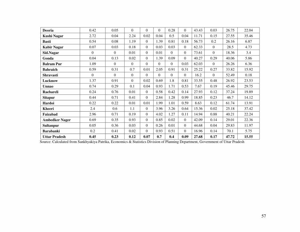
57
Deoria 0.42 0.05 0 0 0 0.28 0 43.43 0.03 26.75 22.04
Kushi Nagar 2.72 0.04 2.24 0.02 0.04 0.5 0.04 11.71 0.15 27.55 35.46
Basti 0.54 0.08 1.19 0 1.39 0.81 0.18 56.73 0.2 26.16 6.87
Kabir Nagar 0.07 0.03 0.18 0 0.03 0.03 0 62.33 0 28.5 4.73
Sid.Nagar 0 0 0.01 0 0.01 0 0 73.61 0 18.36 3.4
Gonda 0.04 0.13 0.02 0 1.39 0.09 0 40.27 0.29 40.06 5.86
Balram Pur 1.09 0 0 0 0 0 0.03 62.03 0 26.26 6.36
Bahraich 0.59 0.31 0.7 0.01 2.05 0.91 0.31 25.22 0.27 33.82 15.92
Shravasti 0 0 0 0 0 0 0 16.2 0 52.49 0.18
Lucknow 1.37 0.91 0 0.02 0.69 1.8 0.81 33.55 0.48 26.92 23.53
Unnao 0.74 0.29 0.1 0.04 0.93 1.71 0.53 7.67 0.19 45.46 29.75
Raebareli 0.24 0.76 0.01 0 0.58 0.42 0.14 27.93 0.12 37.24 19.89
Sitapur 0.44 0.71 0.41 0 2.84 1.28 0.99 18.85 0.23 46.7 14.12
Hardoi 0.22 0.22 0.01 0.01 1.99 1.01 0.59 8.63 0.12 61.74 13.91
Kheeri 2.4 0.6 1.1 0 3.96 3.26 0.64 15.36 0.02 25.18 37.42
Faizabad 2.96 0.71 0.19 0 4.02 1.27 0.11 14.94 0.88 40.21 22.24
Ambedker Nager 0.69 0.35 0.93 0 0.85 0.02 0 42.09 0.14 29.01 22.36
Sultanpur 0.05 0.36 0.03 0 0.26 0.01 0 44.68 0.04 29.83 11.97
Barabanki 0.2 0.41 0.02 0 0.93 0.51 0 16.96 0.14 70.1 5.75
Uttar Pradesh 0.45 0.23 0.12 0.07 0.7 0.4 0.09 27.68 0.17 47.72 15.55
Source: Calculated from Sankhyakiya Patrika, Economics & Statistics Division of Planning Department, Government of Uttar Pradesh
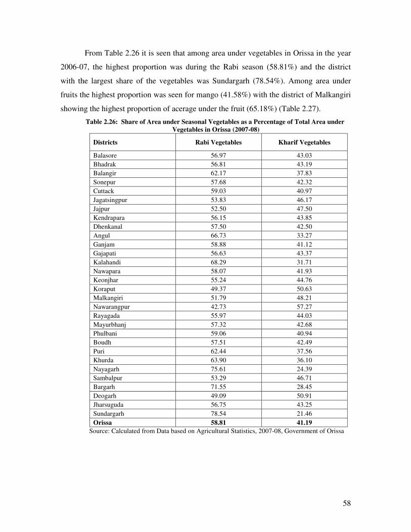
58
From Table 2.26 it is seen that among area under vegetables in Orissa in the year
2006-07, the highest proportion was during the Rabi season (58.81%) and the district
with the largest share of the vegetables was Sundargarh (78.54%). Among area under
fruits the highest proportion was seen for mango (41.58%) with the district of Malkangiri
showing the highest proportion of acerage under the fruit (65.18%) (Table 2.27).
Table 2.26: Share of Area under Seasonal Vegetables as a Percentage of Total Area under
Vegetables in Orissa (2007-08)
Source: Calculated from Data based on Agricultural Statistics, 2007-08, Government of Orissa
Districts Rabi Vegetables Kharif Vegetables
Balasore 56.97 43.03
Bhadrak 56.81 43.19
Balangir 62.17 37.83
Sonepur 57.68 42.32
Cuttack 59.03 40.97
Jagatsingpur 53.83 46.17
Jajpur 52.50 47.50
Kendrapara 56.15 43.85
Dhenkanal 57.50 42.50
Angul 66.73 33.27
Ganjam 58.88 41.12
Gajapati 56.63 43.37
Kalahandi 68.29 31.71
Nawapara 58.07 41.93
Keonjhar 55.24 44.76
Koraput 49.37 50.63
Malkangiri 51.79 48.21
Nawarangpur 42.73 57.27
Rayagada 55.97 44.03
Mayurbhanj 57.32 42.68
Phulbani 59.06 40.94
Boudh 57.51 42.49
Puri 62.44 37.56
Khurda 63.90 36.10
Nayagarh 75.61 24.39
Sambalpur 53.29 46.71
Bargarh 71.55 28.45
Deogarh 49.09 50.91
Jharsuguda 56.75 43.25
Sundargarh 78.54 21.46
Orissa 58.81 41.19
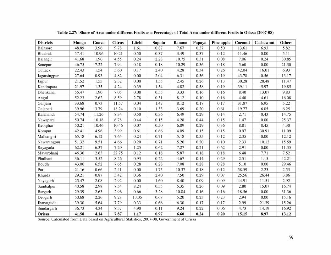
59
Table 2.27: Share of Area under different Fruits as a Percentage of Total Area under different Fruits in Orissa (2007-08)
Districts Mango Guava Citrus Litchi Sapota Banana Papaya Pine apple Coconut Cashewnut Others
Balasore 48.89 3.96 9.78 1.61 0.87 7.67 0.37 0.50 13.61 6.93 5.82
Bhadrak 57.41 10.96 10.21 0.50 0.37 3.49 0.37 0.12 11.46 0.00 5.11
Balangir 41.68 1.96 4.55 0.24 2.28 10.75 0.31 0.08 7.06 0.24 30.85
Sonepur 46.75 7.22 7.94 0.18 0.18 10.29 0.36 0.18 5.60 0.00 21.30
Cuttack 22.43 1.54 3.60 0.17 2.40 4.28 0.34 0.26 42.04 16.01 6.93
Jagatsingpur 27.64 0.93 4.82 0.00 2.04 6.31 0.56 0.19 43.78 0.56 13.17
Jajpur 21.52 1.55 2.32 0.00 1.55 2.45 0.26 0.13 30.28 28.48 11.47
Kendrapara 21.97 1.35 4.24 0.39 1.54 4.82 0.58 0.19 39.11 5.97 19.85
Dhenkanal 55.47 1.90 7.05 0.08 0.55 3.33 0.16 0.16 8.40 13.07 9.83
Angul 52.23 2.62 8.59 2.78 0.31 8.12 0.10 0.16 4.40 4.61 16.08
Ganjam 33.68 0.73 11.57 0.04 1.47 8.12 0.17 0.17 31.87 6.95 5.22
Gajapati 39.96 3.79 18.24 0.10 1.33 3.69 0.20 0.61 19.77 6.05 6.25
Kalahandi 54.74 11.26 8.34 0.50 0.36 6.49 0.29 0.14 2.71 0.43 14.75
Nawapara 50.74 10.18 6.78 0.44 0.15 4.28 0.44 0.15 1.47 0.00 25.37
Keonjhar 50.21 10.46 10.46 0.07 0.50 6.09 0.29 0.36 8.81 8.45 4.30
Koraput 42.41 4.96 3.99 0.61 0.66 4.09 0.15 0.15 0.97 30.91 11.09
Malkangiri 65.18 6.12 7.65 0.24 0.71 5.18 0.35 0.12 2.35 0.00 12.12
Nawarangpur 51.32 9.51 4.66 0.20 0.71 5.26 0.20 0.10 2.33 10.12 15.59
Rayagada 62.21 6.37 7.20 1.25 0.62 7.27 0.21 0.62 2.91 0.00 11.35
Mayurbhanj 46.36 2.63 22.75 0.12 0.18 5.87 0.18 0.18 6.48 7.71 7.52
Phulbani 36.11 3.52 8.26 0.93 0.22 4.67 0.14 0.29 2.51 1.15 42.21
Boudh 43.06 6.52 7.65 0.28 0.28 7.08 0.28 0.28 5.10 0.00 29.46
Puri 21.16 0.66 2.41 0.00 1.75 10.37 0.18 0.12 58.59 2.23 2.53
Khurda 29.21 0.87 3.42 0.36 2.40 7.50 0.29 0.07 25.56 26.44 3.86
Nayagarh 25.47 2.08 2.92 0.00 1.60 8.40 0.09 0.09 44.91 11.51 2.92
Sambalpur 40.58 2.98 7.54 8.24 0.35 5.35 0.26 0.09 2.80 15.07 16.74
Bargarh 29.39 2.63 2.96 0.66 3.28 10.84 0.16 0.16 18.56 0.00 31.36
Deogarh 50.68 2.26 9.28 13.35 0.68 5.20 0.23 0.23 2.94 0.00 15.16
Jharsuguda 39.30 5.64 7.79 0.33 0.66 6.30 0.17 0.17 2.99 21.39 15.26
Sundargarh 36.73 4.34 8.57 4.90 0.11 9.24 0.22 0.06 4.73 14.19 16.92
Orissa 41.58 4.14 7.87 1.17 0.97 6.60 0.24 0.20 15.15 8.97 13.12
Source: Calculated from Data based on Agricultural Statistics, 2007-08, Government of Orissa
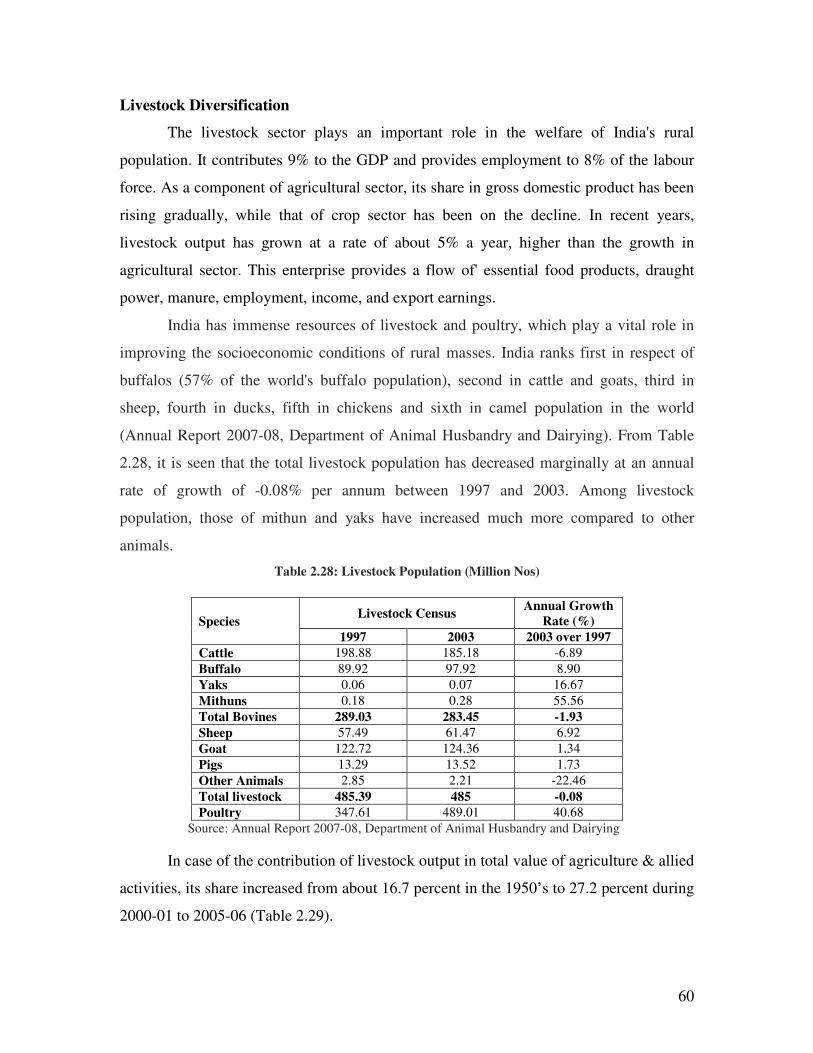
60
Livestock Diversification
The livestock sector plays an important role in the welfare of India's rural
population. It contributes 9% to the GDP and provides employment to 8% of the labour
force. As a component of agricultural sector, its share in gross domestic product has been
rising gradually, while that of crop sector has been on the decline. In recent years,
livestock output has grown at a rate of about 5% a year, higher than the growth in
agricultural sector. This enterprise provides a flow of' essential food products, draught
power, manure, employment, income, and export earnings.
India has immense resources of livestock and poultry, which play a vital role in
improving the socioeconomic conditions of rural masses. India ranks first in respect of
buffalos (57% of the world's buffalo population), second in cattle and goats, third in
sheep, fourth in ducks, fifth in chickens and sixth in camel population in the world
(Annual Report 2007-08, Department of Animal Husbandry and Dairying). From Table
2.28, it is seen that the total livestock population has decreased marginally at an annual
rate of growth of -0.08% per annum between 1997 and 2003. Among livestock
population, those of mithun and yaks have increased much more compared to other
animals.
Table 2.28: Livestock Population (Million Nos)
Species Livestock Census
Annual Growth
Rate (%)
1997 2003 2003 over 1997
Cattle 198.88 185.18 -6.89
Buffalo 89.92 97.92 8.90
Yaks 0.06 0.07 16.67
Mithuns 0.18 0.28 55.56
Total Bovines 289.03 283.45 -1.93
Sheep 57.49 61.47 6.92
Goat 122.72 124.36 1.34
Pigs 13.29 13.52 1.73
Other Animals 2.85 2.21 -22.46
Total livestock 485.39 485 -0.08
Poultry 347.61 489.01 40.68
Source: Annual Report 2007-08, Department of Animal Husbandry and Dairying
In case of the contribution of livestock output in total value of agriculture & allied
activities, its share increased from about 16.7 percent in the 1950’s to 27.2 percent during
2000-01 to 2005-06 (Table 2.29).
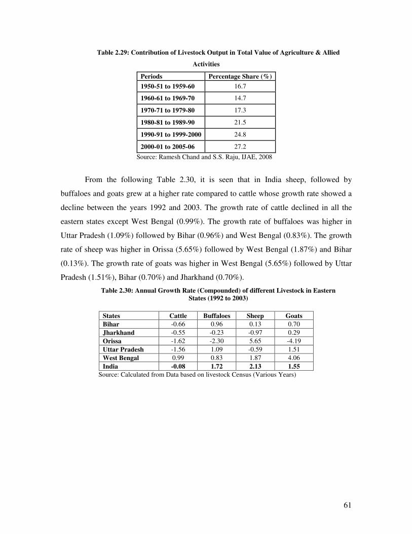
61
Table 2.29: Contribution of Livestock Output in Total Value of Agriculture & Allied
Activities
Periods Percentage Share (%)
1950-51 to 1959-60 16.7
1960-61 to 1969-70 14.7
1970-71 to 1979-80 17.3
1980-81 to 1989-90 21.5
1990-91 to 1999-2000 24.8
2000-01 to 2005-06 27.2
Source: Ramesh Chand and S.S. Raju, IJAE, 2008
From the following Table 2.30, it is seen that in India sheep, followed by
buffaloes and goats grew at a higher rate compared to cattle whose growth rate showed a
decline between the years 1992 and 2003. The growth rate of cattle declined in all the
eastern states except West Bengal (0.99%). The growth rate of buffaloes was higher in
Uttar Pradesh (1.09%) followed by Bihar (0.96%) and West Bengal (0.83%). The growth
rate of sheep was higher in Orissa (5.65%) followed by West Bengal (1.87%) and Bihar
(0.13%). The growth rate of goats was higher in West Bengal (5.65%) followed by Uttar
Pradesh (1.51%), Bihar (0.70%) and Jharkhand (0.70%).
Table 2.30: Annual Growth Rate (Compounded) of different Livestock in Eastern States (1992 to 2003)
States Cattle Buffaloes Sheep Goats
Bihar -0.66 0.96 0.13 0.70
Jharkhand -0.55 -0.23 -0.97 0.29
Orissa -1.62 -2.30 5.65 -4.19
Uttar Pradesh -1.56 1.09 -0.59 1.51
West Bengal 0.99 0.83 1.87 4.06
India -0.08 1.72 2.13 1.55
Source: Calculated from Data based on livestock Census (Various Years)
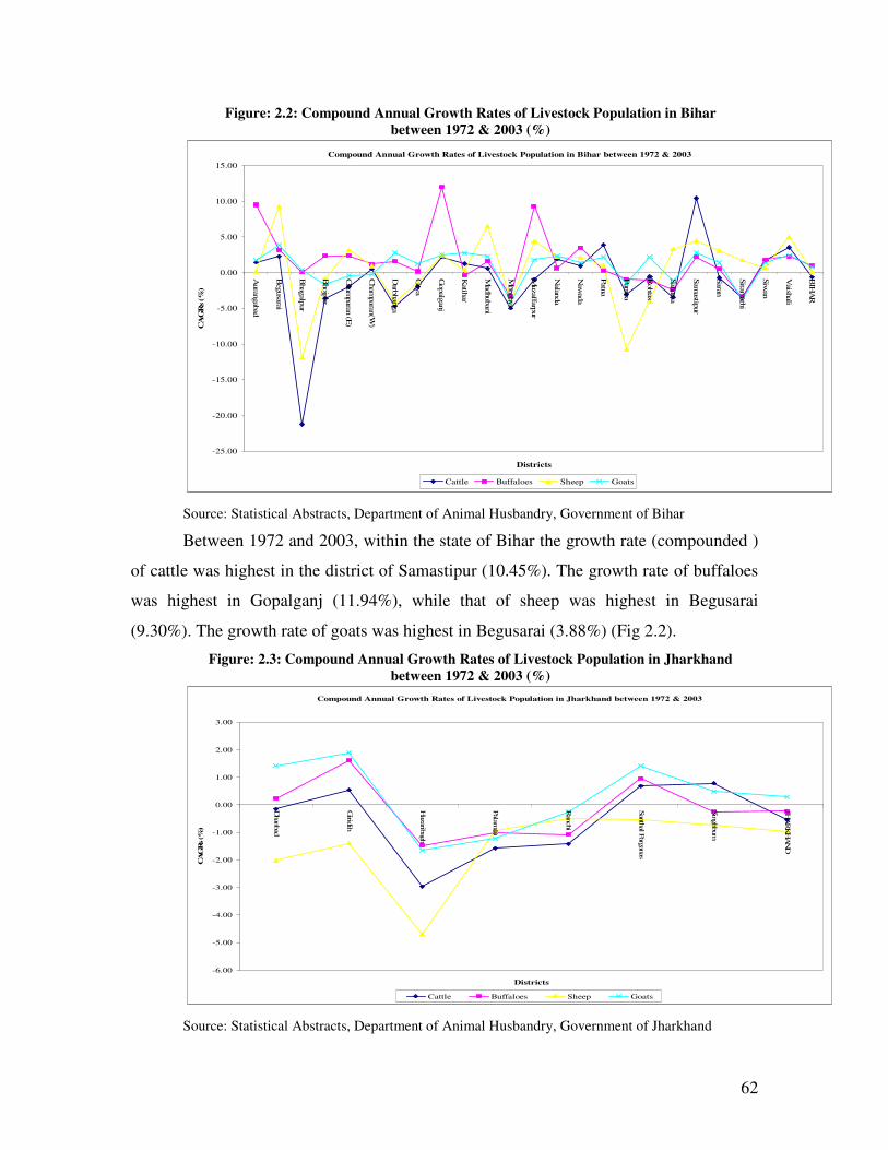
62
Figure: 2.2: Compound Annual Growth Rates of Livestock Population in Bihar
between 1972 & 2003 (%)
Compound Annual Growth Rates of Livestock Population in Bihar between 1972 & 2003
-25.00
-20.00
-15.00
-10.00
-5.00
0.00
5.00
10.00
15.00
Auran
gab
ad
Beg
usarai
Bhag
alpur
Bhojp
ur
Cham
paran
(E)
Cham
paran
(W)
Darb
han
ga
Gay
a
Gopalg
anj
Katih
ar
Mad
huban
i
Monghyr
Muzaffarp
ur
Nalan
da
Naw
ada
Patn
a
Purn
ea
Rohtas
Sah
arsa
Sam
astipur
Saran
Sitam
arhi
Siw
an
Vaish
ali
BIH
AR
Districts
CA
GR
s (%
)
Cattle Buffaloes Sheep Goats
Source: Statistical Abstracts, Department of Animal Husbandry, Government of Bihar
Between 1972 and 2003, within the state of Bihar the growth rate (compounded )
of cattle was highest in the district of Samastipur (10.45%). The growth rate of buffaloes
was highest in Gopalganj (11.94%), while that of sheep was highest in Begusarai
(9.30%). The growth rate of goats was highest in Begusarai (3.88%) (Fig 2.2).
Figure: 2.3: Compound Annual Growth Rates of Livestock Population in Jharkhand
between 1972 & 2003 (%)
Compound Annual Growth Rates of Livestock Population in Jharkhand between 1972 & 2003
-6.00
-5.00
-4.00
-3.00
-2.00
-1.00
0.00
1.00
2.00
3.00
Dhan
bad
Girid
ih
Hazarib
agh
Palam
au
Ran
chi
San
thal P
argan
as
Sin
ghbum
JHA
RK
HA
ND
Districts
CA
GR
s (%
)
Cattle Buffaloes Sheep Goats
Source: Statistical Abstracts, Department of Animal Husbandry, Government of Jharkhand
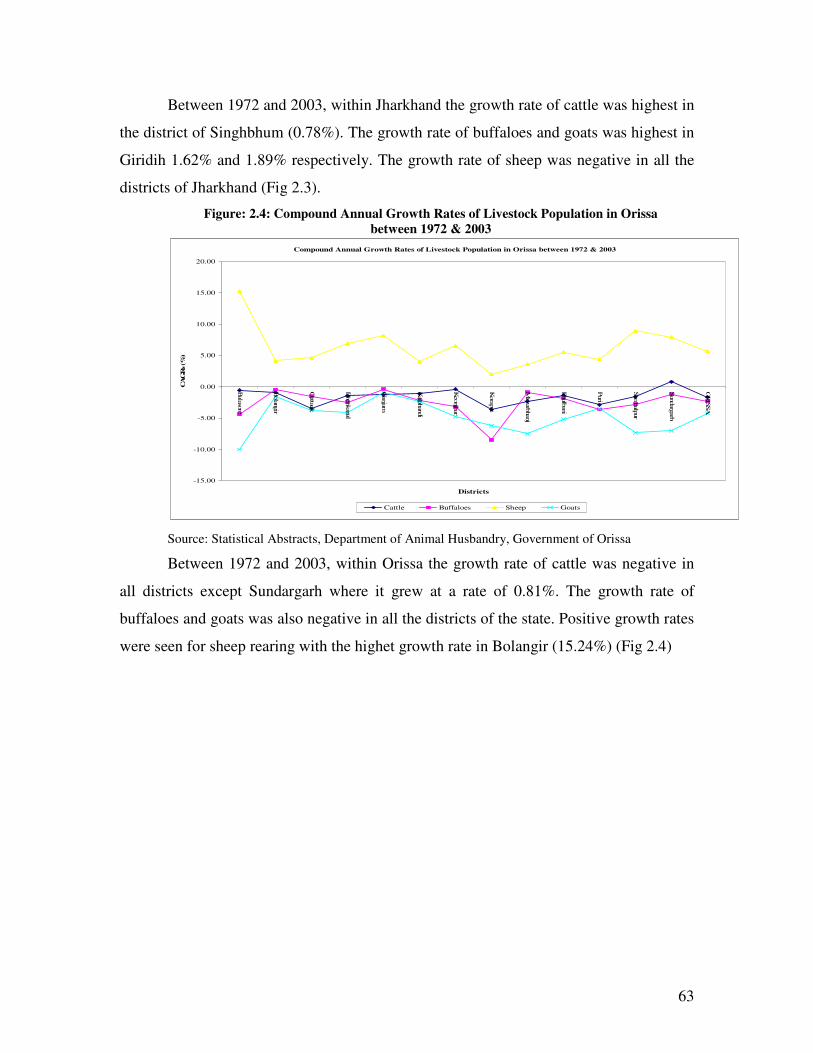
63
Between 1972 and 2003, within Jharkhand the growth rate of cattle was highest in
the district of Singhbhum (0.78%). The growth rate of buffaloes and goats was highest in
Giridih 1.62% and 1.89% respectively. The growth rate of sheep was negative in all the
districts of Jharkhand (Fig 2.3).
Figure: 2.4: Compound Annual Growth Rates of Livestock Population in Orissa
between 1972 & 2003
Compound Annual Growth Rates of Livestock Population in Orissa between 1972 & 2003
-15.00
-10.00
-5.00
0.00
5.00
10.00
15.00
20.00
Balaso
re
Bolan
gir
Cuttac
k
Dhenkanal
Ganjam
Kalah
andi
Keonjh
ar
Kora
put
Mayurb
hanj
Phulb
ani
Puri
Sam
balp
ur
Sundarg
arh
ORIS
SA
Districts
CA
GR
s (%
)
Cattle Buffaloes Sheep Goats
Source: Statistical Abstracts, Department of Animal Husbandry, Government of Orissa
Between 1972 and 2003, within Orissa the growth rate of cattle was negative in
all districts except Sundargarh where it grew at a rate of 0.81%. The growth rate of
buffaloes and goats was also negative in all the districts of the state. Positive growth rates
were seen for sheep rearing with the highet growth rate in Bolangir (15.24%) (Fig 2.4)
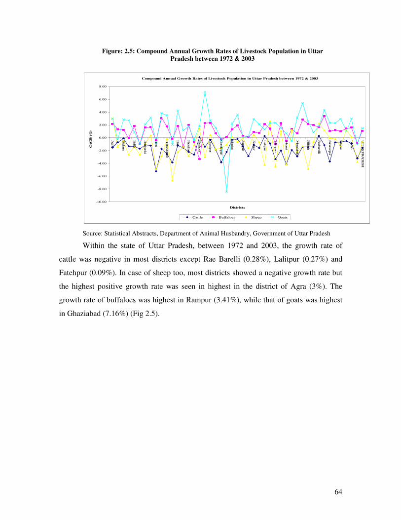
64
Figure: 2.5: Compound Annual Growth Rates of Livestock Population in Uttar
Pradesh between 1972 & 2003
Compound Annual Growth Rates of Livestock Population in Uttar Pradesh between 1972 & 2003
-10.00
-8.00
-6.00
-4.00
-2.00
0.00
2.00
4.00
6.00
8.00
Agra
Bad
aun
Ballia
Barab
anki
Basti
Bullan
dsh
ahr
Etah
Faizab
ad
Fateh
pur
Ghazip
ur
Gorak
hpur
Hard
oi
Jaunpur
Kan
pur
Lalitp
ur
Main
puri
Meeru
t
Morad
abad
Pilib
hit
Raeb
arelli
Sah
aranpur
Sitap
ur
Unnao
UTTA
R P
RA
DESH
Districts
CA
GR
s (%
)
Cattle Buffaloes Sheep Goats
Source: Statistical Abstracts, Department of Animal Husbandry, Government of Uttar Pradesh
Within the state of Uttar Pradesh, between 1972 and 2003, the growth rate of
cattle was negative in most districts except Rae Barelli (0.28%), Lalitpur (0.27%) and
Fatehpur (0.09%). In case of sheep too, most districts showed a negative growth rate but
the highest positive growth rate was seen in highest in the district of Agra (3%). The
growth rate of buffaloes was highest in Rampur (3.41%), while that of goats was highest
in Ghaziabad (7.16%) (Fig 2.5).
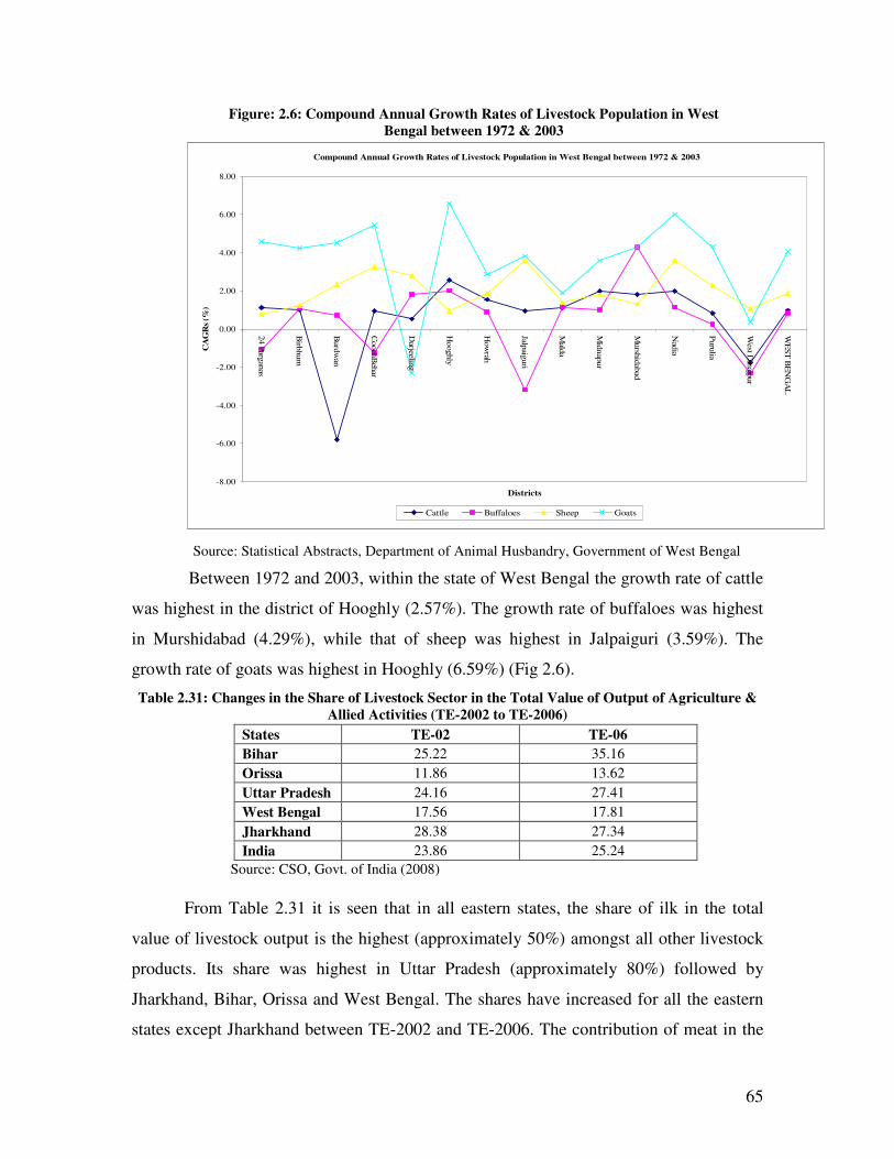
65
Figure: 2.6: Compound Annual Growth Rates of Livestock Population in West
Bengal between 1972 & 2003
Compound Annual Growth Rates of Livestock Population in West Bengal between 1972 & 2003
-8.00
-6.00
-4.00
-2.00
0.00
2.00
4.00
6.00
8.00
24 P
argan
as
Birb
hum
Burd
wan
Cooch
Beh
ar
Darjeelin
g
Hooghly
How
rah
Jalpaig
uri
Mald
a
Mid
nap
ur
Mursh
idab
ad
Nad
ia
Puru
lia
West D
inajp
ur
WE
ST
BE
NG
AL
Districts
CA
GR
s (%
)
Cattle Buffaloes Sheep Goats
Source: Statistical Abstracts, Department of Animal Husbandry, Government of West Bengal
Between 1972 and 2003, within the state of West Bengal the growth rate of cattle
was highest in the district of Hooghly (2.57%). The growth rate of buffaloes was highest
in Murshidabad (4.29%), while that of sheep was highest in Jalpaiguri (3.59%). The
growth rate of goats was highest in Hooghly (6.59%) (Fig 2.6).
Table 2.31: Changes in the Share of Livestock Sector in the Total Value of Output of Agriculture &
Allied Activities (TE-2002 to TE-2006)
Source: CSO, Govt. of India (2008)
From Table 2.31 it is seen that in all eastern states, the share of ilk in the total
value of livestock output is the highest (approximately 50%) amongst all other livestock
products. Its share was highest in Uttar Pradesh (approximately 80%) followed by
Jharkhand, Bihar, Orissa and West Bengal. The shares have increased for all the eastern
states except Jharkhand between TE-2002 and TE-2006. The contribution of meat in the
States TE-02 TE-06
Bihar 25.22 35.16
Orissa 11.86 13.62
Uttar Pradesh 24.16 27.41
West Bengal 17.56 17.81
Jharkhand 28.38 27.34
India 23.86 25.24
66
total value of livestock output is the second highest after milk (approximately 17%). Its
share was highest in West Bengal (approximately 45%) followed by Orissa, Bihar, Uttar
Pradesh and Jharkhand. The shares have declined marginally for most eastern states
except Uttar Pradesh and Jharkhand between TE-2002 and TE-2006.
Table 2.32: Share of Different Items in the Total Value of Livestock Output (TE-2002 to TE-2006)
States
Milk Egg Wool &
Hair Dung
Silk &
Honey Meat
Increment in
Stock
TE-02
TE-06
TE-02
TE-06
TE-02
TE-06
TE-02
TE-06
TE-02
TE-06
TE-02
TE-06
TE-02
TE-06
Bihar 54.34 59.94 1.74 1.32 0.06 0.05 6.93 8.74 0.29 0.09 22.79 17.53 13.84 12.33
Orissa 49.53 52.19 7.19 7.02 0.09 0.07 2.87 1.57 0.55 0.4 34.43 33.92 5.34 4.84
Uttar Pradesh 82.01 82.36 0.51 0.5 0.12 0.11 6.50 5.86 0.03 0.02 11.3 11.45 -0.47 -0.3
West Bengal 44.27 44.65 4.35 4.34 0.07 0.08 4.00 4.14 1.01 1.14 45.04 44.34 1.27 1.3
Jharkhand 67.01 55.44 4.74 6.35 0.18 0.23 19.31 26.47 0.00 0.74 5.74 7.89 3.02 2.89
India 67.8 66.8 3.43 3.57 0.21 0.19 8.10 7.94 1.12 1.04 16.9 17.5 2.4 3.02
Source: CSO, Govt. of India, 2008
Development of Fisheries
Fish production increased in India from 38 lakh tonnes in 1990-91 to 76 lakh
tonnes in 2008-09. Fishing, aquaculture and allied activities are reported to have provided
livelihood to over 14 million persons in 2006-07 apart from being a major foreign
exchange earner (Economic Survey 2009-10).
Till the year 1999-2000, the contribution of marine fisheries in the total fish
production was more than inland fisheries. But its share declined from 60% to 50%
between 1990-91 and 1999-2000. Since the year 2000-01 the situation is just reverse i.e.,
the contribution of inland fisheries is more than marine with the share of the former
increasing from 50% in 2000-01 to 62% in 2008-09 (Fig 2.7).
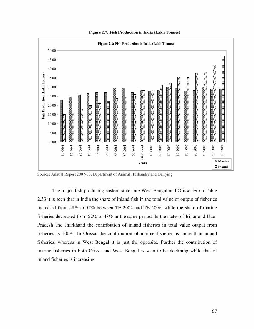
67
Figure 2.7: Fish Production in India (Lakh Tonnes)
Figure 2.2: Fish Production in India (Lakh Tonnes)
0.00
5.00
10.00
15.00
20.00
25.00
30.00
35.00
40.00
45.00
50.00
19
90
-91
19
91
-92
19
92
-93
19
93
-94
19
94
-95
19
95
-96
19
96
-97
19
97
-98
19
98
-99
19
99
-20
00
20
00
-01
20
01
-02
20
02
-03
20
03
-04
20
04
-05
20
05
-06
20
06
-07
20
07
-08
20
08
-09
Years
Fis
h P
rod
uct
ion
(L
ak
h T
on
nes
)
Marine
Inland
Source: Annual Report 2007-08, Department of Animal Husbandry and Dairying
The major fish producing eastern states are West Bengal and Orissa. From Table
2.33 it is seen that in India the share of inland fish in the total value of output of fisheries
increased from 48% to 52% between TE-2002 and TE-2006, while the share of marine
fisheries decreased from 52% to 48% in the same period. In the states of Bihar and Uttar
Pradesh and Jharkhand the contribution of inland fisheries in total value output from
fisheries is 100%. In Orissa, the contribution of marine fisheries is more than inland
fisheries, whereas in West Bengal it is just the opposite. Further the contribution of
marine fisheries in both Orissa and West Bengal is seen to be declining while that of
inland fisheries is increasing.
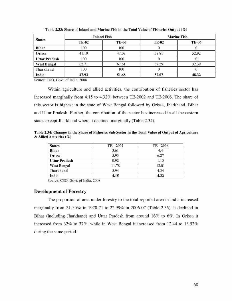
68
Table 2.33: Share of Inland and Marine Fish in the Total Value of Fisheries Output (%)
States Inland Fish Marine Fish
TE-02 TE-06 TE-02 TE-06
Bihar 100 100 0 0
Orissa 41.19 47.08 58.81 52.92
Uttar Pradesh 100 100 0 0
West Bengal 62.71 67.61 37.29 32.39
Jharkhand 100 100 0 0
India 47.93 51.68 52.07 48.32
Source: CSO, Govt. of India, 2008
Within agriculture and allied activities, the contribution of fisheries sector has
increased marginally from 4.15 to 4.32% between TE-2002 and TE-2006. The share of
this sector is highest in the state of West Bengal followed by Orissa, Jharkhand, Bihar
and Uttar Pradesh. Further, the contribution of the sector has increased in all the eastern
states except Jharkhand where it declined marginally (Table 2.34).
Table 2.34: Changes in the Share of Fisheries Sub-Sector in the Total Value of Output of Agriculture
& Allied Activities (%)
Source: CSO, Govt. of India, 2008
Development of Forestry
The proportion of area under forestry to the total reported area in India increased
marginally from 21.55% in 1970-71 to 22.99% in 2006-07 (Table 2.35). It declined in
Bihar (including Jharkhand) and Uttar Pradesh from around 16% to 6%. In Orissa it
increased from 32% to 37%, while in West Bengal it increased from 12.44 to 13.52%
during the same period.
States TE - 2002 TE - 2006
Bihar 3.61 4.4
Orissa 5.95 6.27
Uttar Pradesh 0.92 1.15
West Bengal 11.78 12.01
Jharkhand 5.94 4.34
India 4.15 4.32
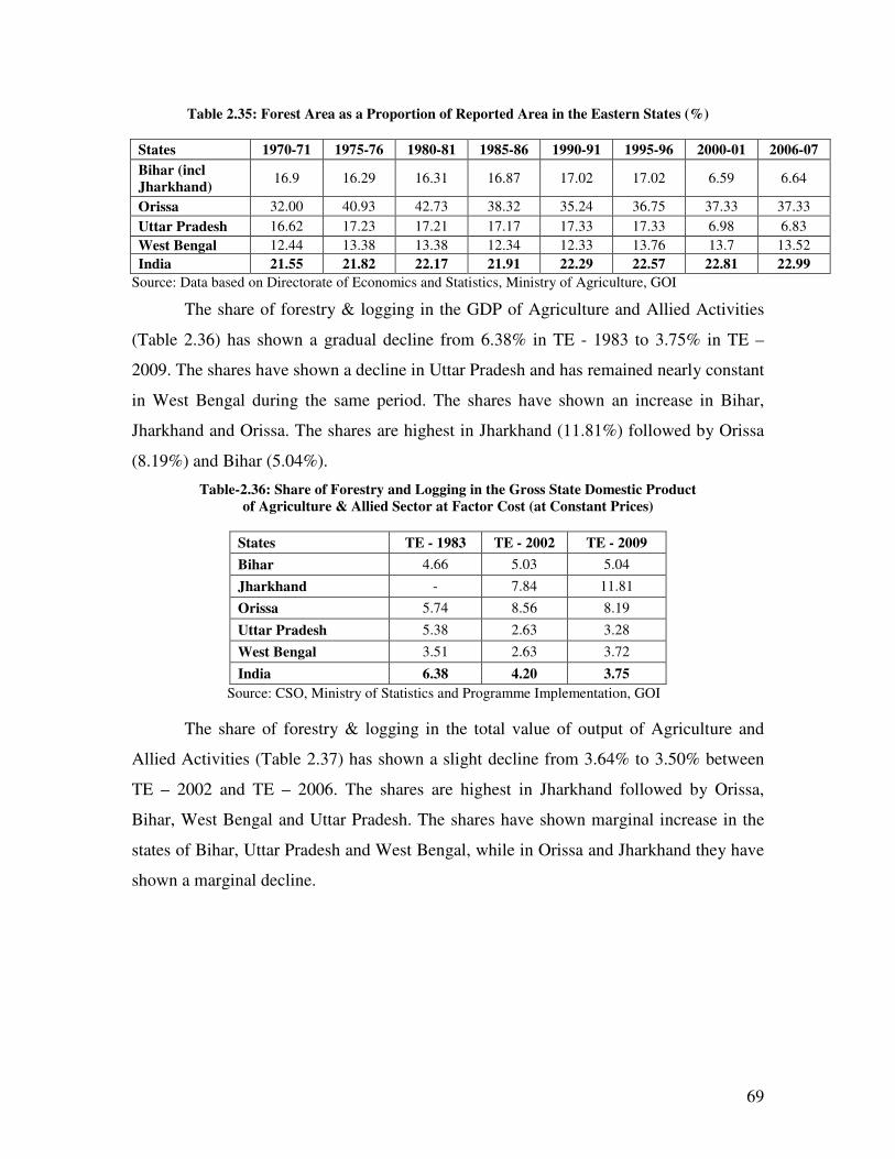
69
Table 2.35: Forest Area as a Proportion of Reported Area in the Eastern States (%)
States 1970-71 1975-76 1980-81 1985-86 1990-91 1995-96 2000-01 2006-07
Bihar (incl Jharkhand)
16.9 16.29 16.31 16.87 17.02 17.02 6.59 6.64
Orissa 32.00 40.93 42.73 38.32 35.24 36.75 37.33 37.33
Uttar Pradesh 16.62 17.23 17.21 17.17 17.33 17.33 6.98 6.83
West Bengal 12.44 13.38 13.38 12.34 12.33 13.76 13.7 13.52
India 21.55 21.82 22.17 21.91 22.29 22.57 22.81 22.99
Source: Data based on Directorate of Economics and Statistics, Ministry of Agriculture, GOI
The share of forestry & logging in the GDP of Agriculture and Allied Activities
(Table 2.36) has shown a gradual decline from 6.38% in TE - 1983 to 3.75% in TE –
2009. The shares have shown a decline in Uttar Pradesh and has remained nearly constant
in West Bengal during the same period. The shares have shown an increase in Bihar,
Jharkhand and Orissa. The shares are highest in Jharkhand (11.81%) followed by Orissa
(8.19%) and Bihar (5.04%).
Table-2.36: Share of Forestry and Logging in the Gross State Domestic Product
of Agriculture & Allied Sector at Factor Cost (at Constant Prices)
States TE - 1983 TE - 2002 TE - 2009
Bihar 4.66 5.03 5.04
Jharkhand - 7.84 11.81
Orissa 5.74 8.56 8.19
Uttar Pradesh 5.38 2.63 3.28
West Bengal 3.51 2.63 3.72
India 6.38 4.20 3.75
Source: CSO, Ministry of Statistics and Programme Implementation, GOI
The share of forestry & logging in the total value of output of Agriculture and
Allied Activities (Table 2.37) has shown a slight decline from 3.64% to 3.50% between
TE – 2002 and TE – 2006. The shares are highest in Jharkhand followed by Orissa,
Bihar, West Bengal and Uttar Pradesh. The shares have shown marginal increase in the
states of Bihar, Uttar Pradesh and West Bengal, while in Orissa and Jharkhand they have
shown a marginal decline.
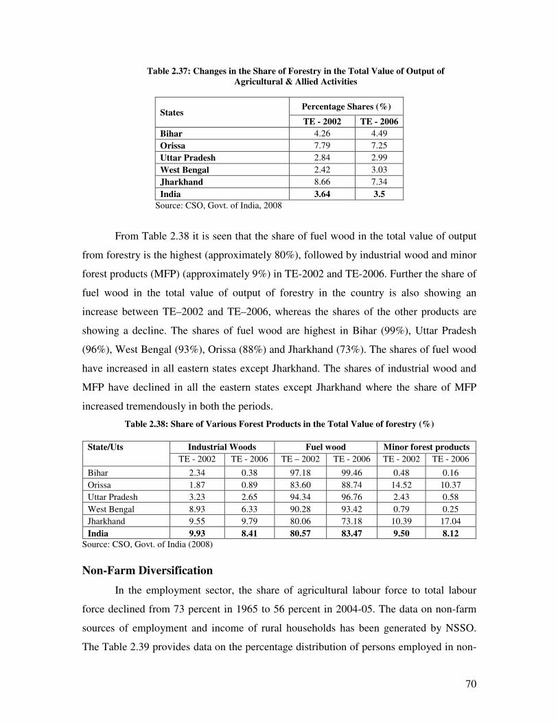
70
Table 2.37: Changes in the Share of Forestry in the Total Value of Output of
Agricultural & Allied Activities
States Percentage Shares (%)
TE - 2002 TE - 2006
Bihar 4.26 4.49
Orissa 7.79 7.25
Uttar Pradesh 2.84 2.99
West Bengal 2.42 3.03
Jharkhand 8.66 7.34
India 3.64 3.5
Source: CSO, Govt. of India, 2008
From Table 2.38 it is seen that the share of fuel wood in the total value of output
from forestry is the highest (approximately 80%), followed by industrial wood and minor
forest products (MFP) (approximately 9%) in TE-2002 and TE-2006. Further the share of
fuel wood in the total value of output of forestry in the country is also showing an
increase between TE–2002 and TE–2006, whereas the shares of the other products are
showing a decline. The shares of fuel wood are highest in Bihar (99%), Uttar Pradesh
(96%), West Bengal (93%), Orissa (88%) and Jharkhand (73%). The shares of fuel wood
have increased in all eastern states except Jharkhand. The shares of industrial wood and
MFP have declined in all the eastern states except Jharkhand where the share of MFP
increased tremendously in both the periods.
Table 2.38: Share of Various Forest Products in the Total Value of forestry (%)
State/Uts Industrial Woods Fuel wood Minor forest products
TE - 2002 TE - 2006 TE – 2002 TE - 2006 TE - 2002 TE - 2006
Bihar 2.34 0.38 97.18 99.46 0.48 0.16
Orissa 1.87 0.89 83.60 88.74 14.52 10.37
Uttar Pradesh 3.23 2.65 94.34 96.76 2.43 0.58
West Bengal 8.93 6.33 90.28 93.42 0.79 0.25
Jharkhand 9.55 9.79 80.06 73.18 10.39 17.04
India 9.93 8.41 80.57 83.47 9.50 8.12
Source: CSO, Govt. of India (2008)
Non-Farm Diversification
In the employment sector, the share of agricultural labour force to total labour
force declined from 73 percent in 1965 to 56 percent in 2004-05. The data on non-farm
sources of employment and income of rural households has been generated by NSSO.
The Table 2.39 provides data on the percentage distribution of persons employed in non-
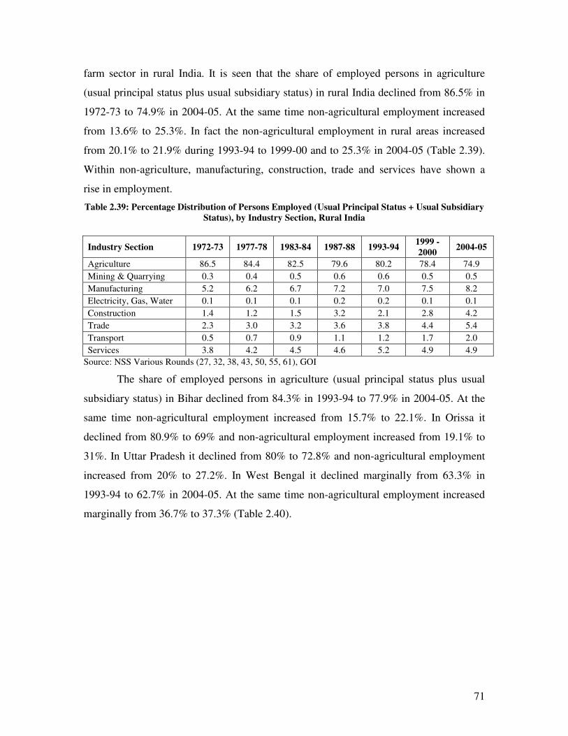
71
farm sector in rural India. It is seen that the share of employed persons in agriculture
(usual principal status plus usual subsidiary status) in rural India declined from 86.5% in
1972-73 to 74.9% in 2004-05. At the same time non-agricultural employment increased
from 13.6% to 25.3%. In fact the non-agricultural employment in rural areas increased
from 20.1% to 21.9% during 1993-94 to 1999-00 and to 25.3% in 2004-05 (Table 2.39).
Within non-agriculture, manufacturing, construction, trade and services have shown a
rise in employment.
Table 2.39: Percentage Distribution of Persons Employed (Usual Principal Status + Usual Subsidiary
Status), by Industry Section, Rural India
Industry Section 1972-73 1977-78 1983-84 1987-88 1993-94 1999 -
2000 2004-05
Agriculture 86.5 84.4 82.5 79.6 80.2 78.4 74.9
Mining & Quarrying 0.3 0.4 0.5 0.6 0.6 0.5 0.5
Manufacturing 5.2 6.2 6.7 7.2 7.0 7.5 8.2
Electricity, Gas, Water 0.1 0.1 0.1 0.2 0.2 0.1 0.1
Construction 1.4 1.2 1.5 3.2 2.1 2.8 4.2
Trade 2.3 3.0 3.2 3.6 3.8 4.4 5.4
Transport 0.5 0.7 0.9 1.1 1.2 1.7 2.0
Services 3.8 4.2 4.5 4.6 5.2 4.9 4.9
Source: NSS Various Rounds (27, 32, 38, 43, 50, 55, 61), GOI
The share of employed persons in agriculture (usual principal status plus usual
subsidiary status) in Bihar declined from 84.3% in 1993-94 to 77.9% in 2004-05. At the
same time non-agricultural employment increased from 15.7% to 22.1%. In Orissa it
declined from 80.9% to 69% and non-agricultural employment increased from 19.1% to
31%. In Uttar Pradesh it declined from 80% to 72.8% and non-agricultural employment
increased from 20% to 27.2%. In West Bengal it declined marginally from 63.3% in
1993-94 to 62.7% in 2004-05. At the same time non-agricultural employment increased
marginally from 36.7% to 37.3% (Table 2.40).
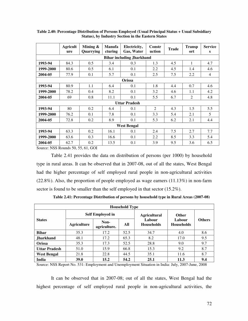
72
Table 2.40: Percentage Distribution of Persons Employed (Usual Principal Status + Usual Subsidiary
Status), by Industry Section in the Eastern States
Agricult
ure
Mining &
Quarrying
Manufa
cturing
Electricity,
Gas, Water
Constr
uction Trade
Transp
ort
Service
s
Bihar including Jharkhand
1993-94 84.3 0.5 3.4 0.3 1.3 4.5 1 4.7
1999-2000 80.6 0.5 6.1 0.1 2.2 4.5 1.4 4.6
2004-05 77.9 0.1 5.7 0.1 2.5 7.5 2.2 4
Orissa
1993-94 80.9 1.1 6.4 0.1 1.8 4.4 0.7 4.6
1999-2000 78.2 0.4 8.2 0.1 3.2 4.6 1.1 4.2
2004-05 69 0.8 11.1 0.1 5.5 6.7 2 4.8
Uttar Pradesh
1993-94 80 0.2 6.4 0.1 2 4.3 1.5 5.5
1999-2000 76.2 0.1 7.8 0.1 3.3 5.4 2.1 5
2004-05 72.8 0.2 8.9 0.1 5.3 6.2 2.1 4.4
West Bengal
1993-94 63.3 0.2 16.1 0.1 2.4 7.5 2.7 7.7
1999-2000 63.6 0.3 16.6 0.1 2.2 8.5 3.3 5.4
2004-05 62.7 0.2 13.5 0.1 3.9 9.5 3.6 6.5
Source: NSS Rounds 50, 55, 61, GOI
Table 2.41 provides the data on distribution of persons (per 1000) by household
type in rural areas. It can be observed that in 2007-08, out of all the states, West Bengal
had the higher percentage of self employed rural people in non-agricultural activities
(22.8%). Also, the proportion of people employed as wage earners (11.13%) in non-farm
sector is found to be smaller than the self employed in that sector (15.2%).
Table 2.41: Percentage Distribution of persons by household type in Rural Areas (2007-08)
Household Type
States
Self Employed in Agricultural
Labour
Households
Other
Labour
Households
Others Agriculture
Non-
agriculture. All
Bihar 35.3 17.2 52.5 34.7 4.0 8.6
Jharkhand 48.1 17.2 65.3 8.2 17.0 9.5
Orissa 35.3 17.3 52.5 28.8 9.0 9.7
Uttar Pradesh 51.0 15.9 66.8 15.3 9.2 8.7
West Bengal 21.8 22.8 44.5 35.1 11.6 8.7
India 39.0 15.2 54.2 25.1 11.3 9.4
Source: NSS Report No. 531: Employment and Unemployment Situation in India: July, 2007-June, 2008
It can be observed that in 2007-08; out of all the states, West Bengal had the
highest percentage of self employed rural people in non-agricultural activities, the
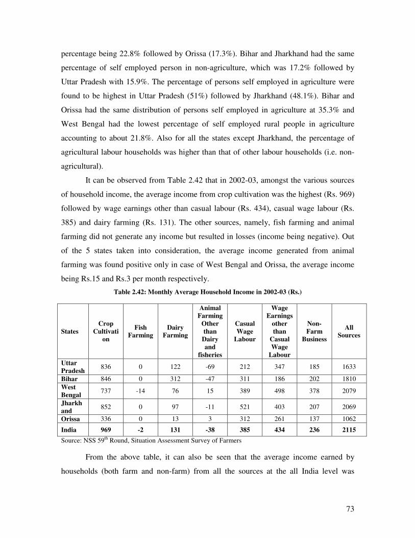
73
percentage being 22.8% followed by Orissa (17.3%). Bihar and Jharkhand had the same
percentage of self employed person in non-agriculture, which was 17.2% followed by
Uttar Pradesh with 15.9%. The percentage of persons self employed in agriculture were
found to be highest in Uttar Pradesh (51%) followed by Jharkhand (48.1%). Bihar and
Orissa had the same distribution of persons self employed in agriculture at 35.3% and
West Bengal had the lowest percentage of self employed rural people in agriculture
accounting to about 21.8%. Also for all the states except Jharkhand, the percentage of
agricultural labour households was higher than that of other labour households (i.e. non-
agricultural).
It can be observed from Table 2.42 that in 2002-03, amongst the various sources
of household income, the average income from crop cultivation was the highest (Rs. 969)
followed by wage earnings other than casual labour (Rs. 434), casual wage labour (Rs.
385) and dairy farming (Rs. 131). The other sources, namely, fish farming and animal
farming did not generate any income but resulted in losses (income being negative). Out
of the 5 states taken into consideration, the average income generated from animal
farming was found positive only in case of West Bengal and Orissa, the average income
being Rs.15 and Rs.3 per month respectively.
Table 2.42: Monthly Average Household Income in 2002-03 (Rs.)
States
Crop
Cultivation
Fish Farming
Dairy Farming
Animal
Farming
Other
than Dairy
and
fisheries
Casual
Wage Labour
Wage
Earnings
other
than Casual
Wage
Labour
Non-
Farm Business
All Sources
Uttar
Pradesh 836 0 122 -69 212 347 185 1633
Bihar 846 0 312 -47 311 186 202 1810
West
Bengal 737 -14 76 15 389 498 378 2079
Jharkhand
852 0 97 -11 521 403 207 2069
Orissa 336 0 13 3 312 261 137 1062
India 969 -2 131 -38 385 434 236 2115
Source: NSS 59th
Round, Situation Assessment Survey of Farmers
From the above table, it can also be seen that the average income earned by
households (both farm and non-farm) from all the sources at the all India level was
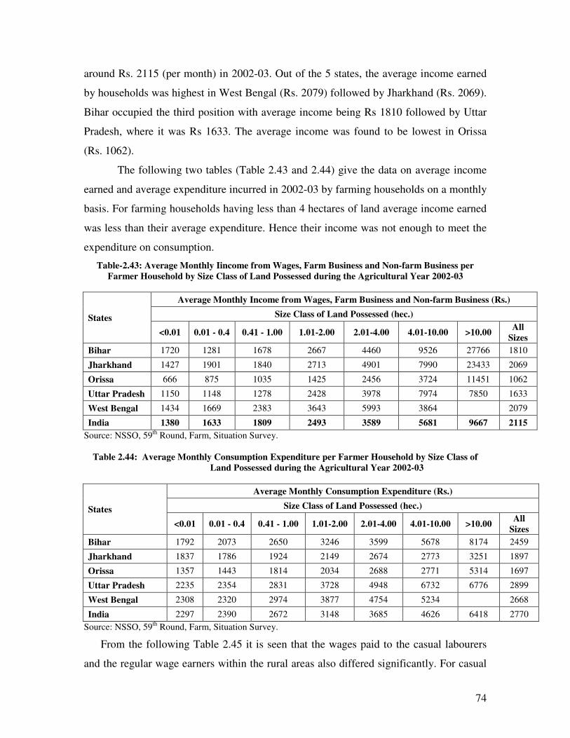
74
around Rs. 2115 (per month) in 2002-03. Out of the 5 states, the average income earned
by households was highest in West Bengal (Rs. 2079) followed by Jharkhand (Rs. 2069).
Bihar occupied the third position with average income being Rs 1810 followed by Uttar
Pradesh, where it was Rs 1633. The average income was found to be lowest in Orissa
(Rs. 1062).
The following two tables (Table 2.43 and 2.44) give the data on average income
earned and average expenditure incurred in 2002-03 by farming households on a monthly
basis. For farming households having less than 4 hectares of land average income earned
was less than their average expenditure. Hence their income was not enough to meet the
expenditure on consumption.
Table-2.43: Average Monthly Iincome from Wages, Farm Business and Non-farm Business per
Farmer Household by Size Class of Land Possessed during the Agricultural Year 2002-03
States
Average Monthly Income from Wages, Farm Business and Non-farm Business (Rs.)
Size Class of Land Possessed (hec.)
<0.01 0.01 - 0.4 0.41 - 1.00 1.01-2.00 2.01-4.00 4.01-10.00 >10.00 All
Sizes
Bihar 1720 1281 1678 2667 4460 9526 27766 1810
Jharkhand 1427 1901 1840 2713 4901 7990 23433 2069
Orissa 666 875 1035 1425 2456 3724 11451 1062
Uttar Pradesh 1150 1148 1278 2428 3978 7974 7850 1633
West Bengal 1434 1669 2383 3643 5993 3864 2079
India 1380 1633 1809 2493 3589 5681 9667 2115
Source: NSSO, 59th
Round, Farm, Situation Survey.
Table 2.44: Average Monthly Consumption Expenditure per Farmer Household by Size Class of
Land Possessed during the Agricultural Year 2002-03
States
Average Monthly Consumption Expenditure (Rs.)
Size Class of Land Possessed (hec.)
<0.01 0.01 - 0.4 0.41 - 1.00 1.01-2.00 2.01-4.00 4.01-10.00 >10.00 All
Sizes
Bihar 1792 2073 2650 3246 3599 5678 8174 2459
Jharkhand 1837 1786 1924 2149 2674 2773 3251 1897
Orissa 1357 1443 1814 2034 2688 2771 5314 1697
Uttar Pradesh 2235 2354 2831 3728 4948 6732 6776 2899
West Bengal 2308 2320 2974 3877 4754 5234 2668
India 2297 2390 2672 3148 3685 4626 6418 2770
Source: NSSO, 59th
Round, Farm, Situation Survey.
From the following Table 2.45 it is seen that the wages paid to the casual labourers
and the regular wage earners within the rural areas also differed significantly. For casual
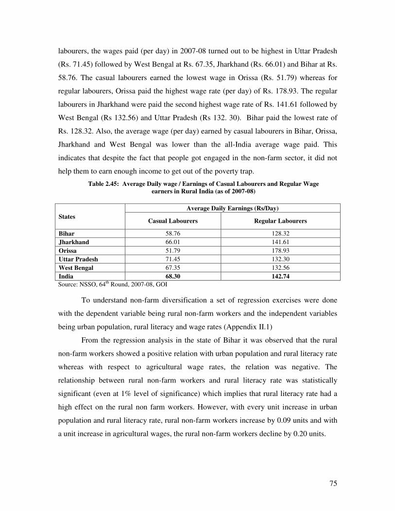
75
labourers, the wages paid (per day) in 2007-08 turned out to be highest in Uttar Pradesh
(Rs. 71.45) followed by West Bengal at Rs. 67.35, Jharkhand (Rs. 66.01) and Bihar at Rs.
58.76. The casual labourers earned the lowest wage in Orissa (Rs. 51.79) whereas for
regular labourers, Orissa paid the highest wage rate (per day) of Rs. 178.93. The regular
labourers in Jharkhand were paid the second highest wage rate of Rs. 141.61 followed by
West Bengal (Rs 132.56) and Uttar Pradesh (Rs 132. 30). Bihar paid the lowest rate of
Rs. 128.32. Also, the average wage (per day) earned by casual labourers in Bihar, Orissa,
Jharkhand and West Bengal was lower than the all-India average wage paid. This
indicates that despite the fact that people got engaged in the non-farm sector, it did not
help them to earn enough income to get out of the poverty trap.
Table 2.45: Average Daily wage / Earnings of Casual Labourers and Regular Wage
earners in Rural India (as of 2007-08)
States
Average Daily Earnings (Rs/Day)
Casual Labourers Regular Labourers
Bihar 58.76 128.32
Jharkhand 66.01 141.61
Orissa 51.79 178.93
Uttar Pradesh 71.45 132.30
West Bengal 67.35 132.56
India 68.30 142.74
Source: NSSO, 64th
Round, 2007-08, GOI
To understand non-farm diversification a set of regression exercises were done
with the dependent variable being rural non-farm workers and the independent variables
being urban population, rural literacy and wage rates (Appendix II.1)
From the regression analysis in the state of Bihar it was observed that the rural
non-farm workers showed a positive relation with urban population and rural literacy rate
whereas with respect to agricultural wage rates, the relation was negative. The
relationship between rural non-farm workers and rural literacy rate was statistically
significant (even at 1% level of significance) which implies that rural literacy rate had a
high effect on the rural non farm workers. However, with every unit increase in urban
population and rural literacy rate, rural non-farm workers increase by 0.09 units and with
a unit increase in agricultural wages, the rural non-farm workers decline by 0.20 units.
76
The relation with respect to urban population and agricultural wages holds true
because as there is increase in urban population it means increase in work opportunities
which in turn can lead to increase in rural non-farm workers. And also with increase in
agricultural wages, people would like to move to agricultural sector leading to decline in
rural non-farm workforce.
For Jharkhand, the relationship with respect to urban population and wage rates
was same as that of Bihar, whereas with respect to rural literacy rate the relationship was
negative. In this case, the relation between rural non farm workers and urban population
was statistically significant (at 1% level of significance) implying that urban population
had a high effect on rural non-farm workforce. A unit increase in rural literacy rate and
agricultural wages, rural non-farm workers decline by 0.60 and 0.41 units respectively.
In case of Orissa and Uttar Pradesh, the scenario is very much similar; the
difference lies in that fact that in Uttar Pradesh, urban population was statistically
significant, hence urban population had a high effect on rural non farm workforce over
there, whereas a unit increase in urban population increased the rural non-farm workforce
by 0.25 and0.35 units in Orissa. However, increase in rural literacy rate and agricultural
wage rates lead to an increase in rural non-farm workforce by 0.70 and 0.08 units in
Orissa and 0.59 and 0.26 units in Uttar Pradesh.
One reason as to why agricultural wage rates explain contradictory result can be
attributed to the exclusion of some of the important variables (like urban wage rate or non
farm wage rate) which could have an impact on the rural non-farm workers.
The relationship in West Bengal is similar to that of Bihar. A unit increase in
urban population and rural literacy rate leads to an increase in rural non-farm workforce
by 0.41 and 0.25 units respectively. While a unit increase in agricultural wage rates
results in a decline in rural non-farm workforce by 0.18 units.
Agro-Based Industries
The industries that add value to agricultural raw materials, both food and non food
(by processing and preserving them for consumption); and at the same time enhance the
income of the producers are called agro based industries. These industries can be
characterized into food-processing industry, livestock industry, fisheries industry and
forestry industry. Amongst these industries; it is the food processing industry which
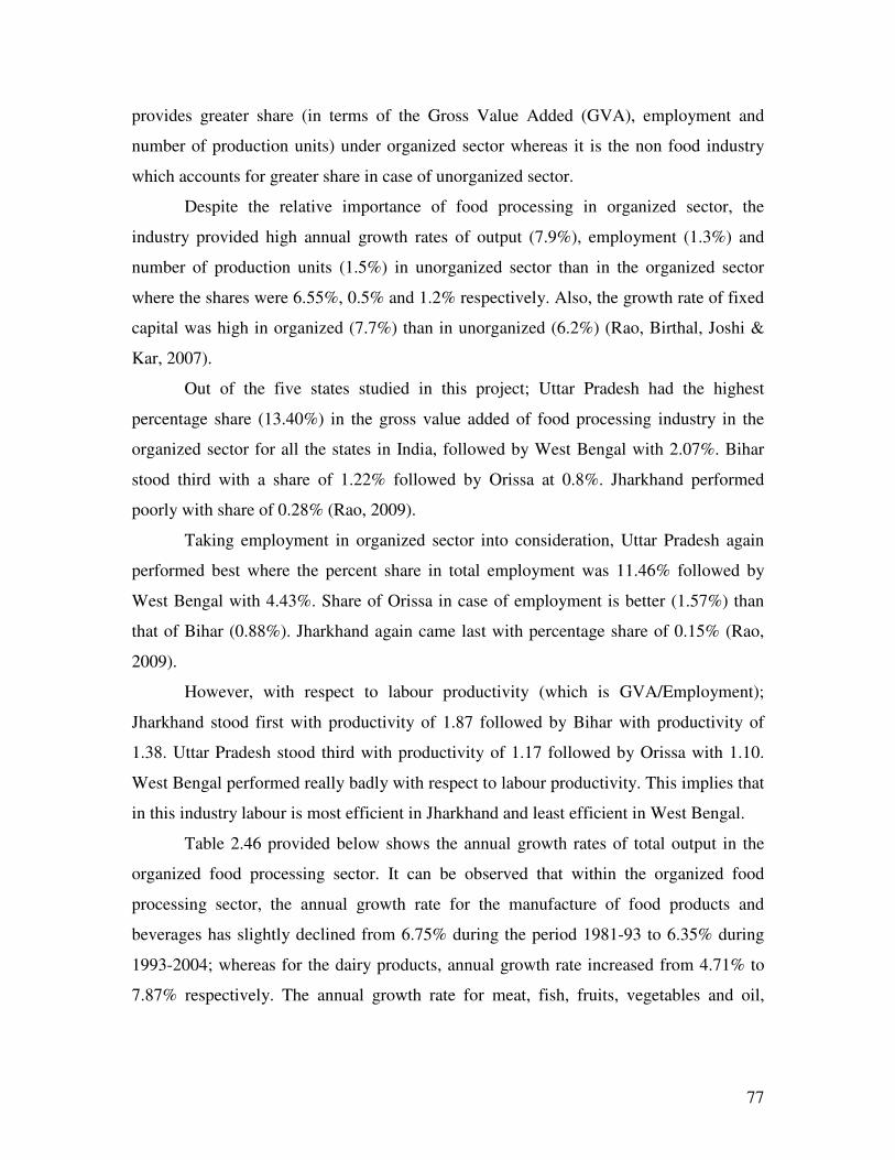
77
provides greater share (in terms of the Gross Value Added (GVA), employment and
number of production units) under organized sector whereas it is the non food industry
which accounts for greater share in case of unorganized sector.
Despite the relative importance of food processing in organized sector, the
industry provided high annual growth rates of output (7.9%), employment (1.3%) and
number of production units (1.5%) in unorganized sector than in the organized sector
where the shares were 6.55%, 0.5% and 1.2% respectively. Also, the growth rate of fixed
capital was high in organized (7.7%) than in unorganized (6.2%) (Rao, Birthal, Joshi &
Kar, 2007).
Out of the five states studied in this project; Uttar Pradesh had the highest
percentage share (13.40%) in the gross value added of food processing industry in the
organized sector for all the states in India, followed by West Bengal with 2.07%. Bihar
stood third with a share of 1.22% followed by Orissa at 0.8%. Jharkhand performed
poorly with share of 0.28% (Rao, 2009).
Taking employment in organized sector into consideration, Uttar Pradesh again
performed best where the percent share in total employment was 11.46% followed by
West Bengal with 4.43%. Share of Orissa in case of employment is better (1.57%) than
that of Bihar (0.88%). Jharkhand again came last with percentage share of 0.15% (Rao,
2009).
However, with respect to labour productivity (which is GVA/Employment);
Jharkhand stood first with productivity of 1.87 followed by Bihar with productivity of
1.38. Uttar Pradesh stood third with productivity of 1.17 followed by Orissa with 1.10.
West Bengal performed really badly with respect to labour productivity. This implies that
in this industry labour is most efficient in Jharkhand and least efficient in West Bengal.
Table 2.46 provided below shows the annual growth rates of total output in the
organized food processing sector. It can be observed that within the organized food
processing sector, the annual growth rate for the manufacture of food products and
beverages has slightly declined from 6.75% during the period 1981-93 to 6.35% during
1993-2004; whereas for the dairy products, annual growth rate increased from 4.71% to
7.87% respectively. The annual growth rate for meat, fish, fruits, vegetables and oil,
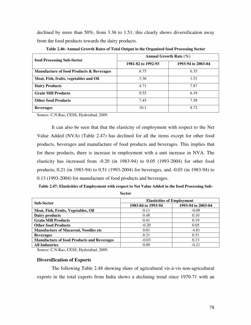
78
declined by more than 50%, from 3.36 to 1.51; this clearly shows diversification away
from the food products towards the dairy products.
Table 2.46: Annual Growth Rates of Total Output in the Organized food Processing Sector
food Processing Sub-Sector Annual Growth Rate (%)
1981-82 to 1992-93 1993-94 to 2003-04
Manufacture of food Products & Beverages 6.75 6.35
Meat, Fish, fruits, vegetables and Oil 3.36 1.51
Dairy Products 4.71 7.87
Grain Mill Products 9.55 6.19
Other food Products 7.45 7.58
Beverages 10.1 8.72
Source: C.N.Rao, CESS, Hyderabad, 2009.
It can also be seen that that the elasticity of employment with respect to the Net
Value Added (NVA) (Table 2.47) has declined for all the items except for other food
products, beverages and manufacture of food products and beverages. This implies that
for these products, there is increase in employment with a unit increase in NVA. The
elasticity has increased from -0.20 (in 1983-94) to 0.05 (1993-2004) for other food
products; 0.21 (in 1983-94) to 0.51 (1993-2004) for beverages, and -0.03 (in 1983-94) to
0.13 (1993-2004) for manufacture of food products and beverages.
Table 2.47: Elasticities of Employment with respect to Net Value Added in the food Processing Sub-
Sector
Sub-Sector Elasticities of Employment
1983-84 to 1993-94 1993-94 to 2003-04
Meat, Fish, Fruits, Vegetables, Oil 0.11 -0.09
Dairy products 0.48 0.10
Grain Mill Products 0.41 0.19
Other food Products -0.20 0.05
Manufacture of Macaroni, Noodles etc 0.01 -4.81
Beverages 0.21 0.51
Manufacture of food Products and Beverages -0.03 0.13
All Industries 0.09 -0.21
Source: C.N.Rao, CESS, Hyderabad, 2009.
Diversification of Exports
The following Table 2.48 showing share of agricultural vis-à-vis non-agricultural
exports in the total exports from India shows a declining trend since 1970-71 with an
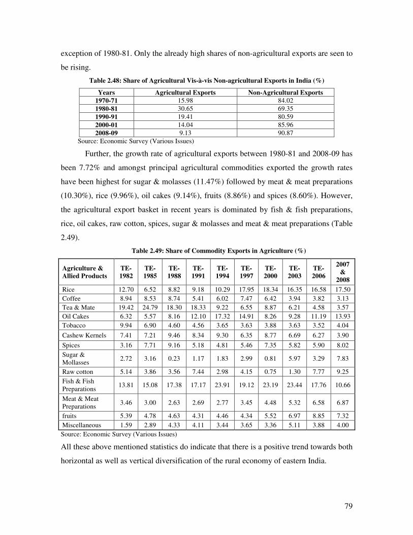
79
exception of 1980-81. Only the already high shares of non-agricultural exports are seen to
be rising.
Table 2.48: Share of Agricultural Vis-à-vis Non-agricultural Exports in India (%)
Years Agricultural Exports Non-Agricultural Exports
1970-71 15.98 84.02
1980-81 30.65 69.35
1990-91 19.41 80.59
2000-01 14.04 85.96
2008-09 9.13 90.87
Source: Economic Survey (Various Issues)
Further, the growth rate of agricultural exports between 1980-81 and 2008-09 has
been 7.72% and amongst principal agricultural commodities exported the growth rates
have been highest for sugar & molasses (11.47%) followed by meat & meat preparations
(10.30%), rice (9.96%), oil cakes (9.14%), fruits (8.86%) and spices (8.60%). However,
the agricultural export basket in recent years is dominated by fish & fish preparations,
rice, oil cakes, raw cotton, spices, sugar & molasses and meat & meat preparations (Table
2.49).
Table 2.49: Share of Commodity Exports in Agriculture (%)
Agriculture & Allied Products
TE-1982
TE-1985
TE-1988
TE-1991
TE-1994
TE-1997
TE-2000
TE-2003
TE-2006
2007 &
2008
Rice 12.70 6.52 8.82 9.18 10.29 17.95 18.34 16.35 16.58 17.50
Coffee 8.94 8.53 8.74 5.41 6.02 7.47 6.42 3.94 3.82 3.13
Tea & Mate 19.42 24.79 18.30 18.33 9.22 6.55 8.87 6.21 4.58 3.57
Oil Cakes 6.32 5.57 8.16 12.10 17.32 14.91 8.26 9.28 11.19 13.93
Tobacco 9.94 6.90 4.60 4.56 3.65 3.63 3.88 3.63 3.52 4.04
Cashew Kernels 7.41 7.21 9.46 8.34 9.30 6.35 8.77 6.69 6.27 3.90
Spices 3.16 7.71 9.16 5.18 4.81 5.46 7.35 5.82 5.90 8.02
Sugar &
Mollasses 2.72 3.16 0.23 1.17 1.83 2.99 0.81 5.97 3.29 7.83
Raw cotton 5.14 3.86 3.56 7.44 2.98 4.15 0.75 1.30 7.77 9.25
Fish & Fish
Preparations 13.81 15.08 17.38 17.17 23.91 19.12 23.19 23.44 17.76 10.66
Meat & Meat
Preparations 3.46 3.00 2.63 2.69 2.77 3.45 4.48 5.32 6.58 6.87
fruits 5.39 4.78 4.63 4.31 4.46 4.34 5.52 6.97 8.85 7.32
Miscellaneous 1.59 2.89 4.33 4.11 3.44 3.65 3.36 5.11 3.88 4.00
Source: Economic Survey (Various Issues)
All these above mentioned statistics do indicate that there is a positive trend towards both
horizontal as well as vertical diversification of the rural economy of eastern India.
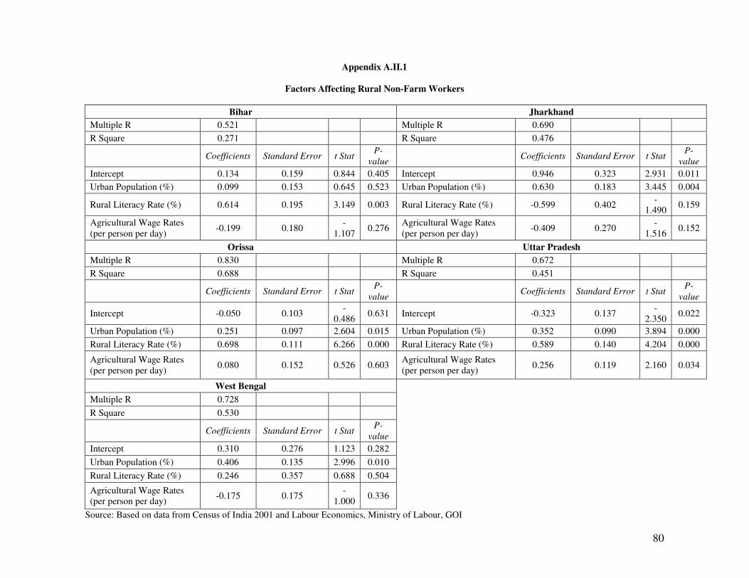
80
Appendix A.II.1
Factors Affecting Rural Non-Farm Workers
Bihar Jharkhand
Multiple R 0.521 Multiple R 0.690
R Square 0.271 R Square 0.476
Coefficients Standard Error t Stat P-
value Coefficients Standard Error t Stat
P-
value
Intercept 0.134 0.159 0.844 0.405 Intercept 0.946 0.323 2.931 0.011
Urban Population (%) 0.099 0.153 0.645 0.523 Urban Population (%) 0.630 0.183 3.445 0.004
Rural Literacy Rate (%) 0.614 0.195 3.149 0.003 Rural Literacy Rate (%) -0.599 0.402 -
1.490 0.159
Agricultural Wage Rates
(per person per day) -0.199 0.180
-
1.107 0.276
Agricultural Wage Rates
(per person per day) -0.409 0.270
-
1.516 0.152
Orissa Uttar Pradesh
Multiple R 0.830 Multiple R 0.672
R Square 0.688 R Square 0.451
Coefficients Standard Error t Stat P-
value Coefficients Standard Error t Stat
P-
value
Intercept -0.050 0.103 -
0.486 0.631 Intercept -0.323 0.137
-
2.350 0.022
Urban Population (%) 0.251 0.097 2.604 0.015 Urban Population (%) 0.352 0.090 3.894 0.000
Rural Literacy Rate (%) 0.698 0.111 6.266 0.000 Rural Literacy Rate (%) 0.589 0.140 4.204 0.000
Agricultural Wage Rates
(per person per day) 0.080 0.152 0.526 0.603
Agricultural Wage Rates
(per person per day) 0.256 0.119 2.160 0.034
West Bengal
Multiple R 0.728
R Square 0.530
Coefficients Standard Error t Stat P-
value
Intercept 0.310 0.276 1.123 0.282
Urban Population (%) 0.406 0.135 2.996 0.010
Rural Literacy Rate (%) 0.246 0.357 0.688 0.504
Agricultural Wage Rates
(per person per day) -0.175 0.175
-
1.000 0.336
Source: Based on data from Census of India 2001 and Labour Economics, Ministry of Labour, GOI
81
CHAPTER III
PRODUCTION STRUCTURE, PROFITABILITY, INCOME
AND VIABILITY OF SMALL AND MARGINAL FARMS
(RESULTS OF FARM LEVEL SURVEY)
A survey of cultivating households was conducted in the states of Uttar Pradesh,
Bihar, West Bengal, Jharkhand and Orissa to study their economics of production and
resource use efficiency. In this chapter some aspects of the production structure of the
selected farming households shall be discussed.
Share of Farming Households Cultivating Different Crops
The following Table 3.1 shows the shares of sample farming households
cultivating different crops as a proportion of the total number of households in each farm
size category in the different states of eastern India. It was observed that farmers in the
study regions mainly cultivated cereals (paddy, maize, wheat, bajra, ragi and jowar),
pulses (khesari or grass pea, arhar, masoor, moong, gram, pea and urad), oilseeds
(mustard, sesame, linseed), vegetables, jute and sugarcane. The cultivation of fruits and
flowers was rarely observed.
It was seen that cereals were cultivated by all sample farming households (100%)
across all farm size categories in all the states. In Bihar most sample farming households
cultivated cereals followed by pulses, oilseeds, vegetables and jute. The developed
district of Rohtas followed a similar pattern, even across farm size categories but in the
underdeveloped district of Kishanganj, cultivation of cereals was followed by that of
oilseeds, jute, pulses and vegetables. 13% of the sample farming households in the
Kishanganj district of Bihar cultivated jute. The district of Kishanganj in Bihar is
bordering West Bengal and hence jute cultivation was found among some sample
farming households here. Across farm sizes it is seen that the proportion of pulses,
oilseeds and vegetables cultivated by small and marginal farmers is lesser when
compared with those cultivated by medium and large farmers.
In Jharkhand most sample farming households cultivated cereals followed by
pulses, sugarcane, vegetables and oilseeds. Both the developed and underdeveloped
districts of Sahebgunj and Lohardaga respectively, followed a similar pattern, except that
82
in Lohardaga, none of the households cultivated sugarcane. This pattern was similar
across farm size categories. Sugarcane was cultivated by 27% of the sample farming
households in the relatively developed district of Sahebganj. Across farm sizes it is seen
that the proportion of each crop cultivated by marginal farmers is very less when
compared to other farm categories. It is 12.15% for pulses, 0.93% for oilseeds and 5.61%
for sugarcane ad vegetables. However, in Jharkhand the proportion of medium farmers
cultivating each crop was the highest. The proportion of large farmers cultivating each
crop was slightly lower than medium farmers. Infact their proportions were nearly similar
to those of small farmers.
In Orissa most sample farming households cultivated cereals followed by
vegetables, oilseeds, pulses and jute. The developed district of Bhadrak followed a
similar pattern, even across farm size categories but in the underdeveloped district of
Kandhamal, cultivation of cereals was followed by that of vegetables, pulses, oilseeds
and jute. Across farm sizes it is seen that the proportion of pulses, oilseeds jute and
vegetables cultivated by small and marginal farmers is lesser than those cultivated by
medium and large farmers.
In Uttar Pradesh most sample farming households cultivated cereals followed by
vegetables, oilseeds, sugarcane and pulses. The developed district of Varanasi followed a
similar pattern, even across farm size categories but in the underdeveloped district of
Mirzapur, cultivation of cereals was followed by oilseeds and pulses only. This pattern
here too was similar across farming categories. Across farm sizes it is seen that the
proportion of pulses, oilseeds and sugarcane cultivated by small and marginal farmers is
lesser as compared to those cultivated by medium and large farmers In case of vegetables
it is seen that a very small proportion of large farmers are cultivating it (14%).
In West Bengal most sample farming households cultivated cereals followed by
oilseeds, vegetables and jute. The developed district of Burdwan followed a similar
pattern, even across farm size categories but in the underdeveloped district of Jalpaiguri
cultivation of cereals was followed by oilseeds, jute and vegetables. This pattern here too
was similar across farming categories. Across farm sizes it is seen that the proportion of
oilseeds, jute and vegetables cultivated by small and marginal farmers is much lesser
compared with those cultivated by medium and large farmers.
83
Thus, it is to be noted that a small proportion of small and marginal farming
households in all the study regions cultivated high value crops other than Food grains
(oilseeds, vegetables and plantation crops). While a high proportion of medium and large
farming households cultivated these high value crops.
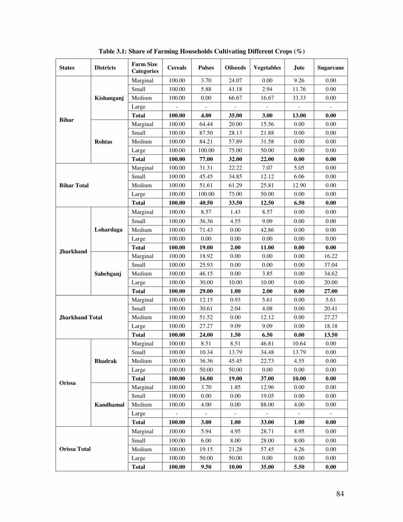
84
Table 3.1: Share of Farming Households Cultivating Different Crops (%)
States Districts Farm Size Categories
Cereals Pulses Oilseeds Vegetables Jute Sugarcane
Bihar
Kishanganj
Marginal 100.00 3.70 24.07 0.00 9.26 0.00
Small 100.00 5.88 41.18 2.94 11.76 0.00
Medium 100.00 0.00 66.67 16.67 33.33 0.00
Large - - - - - -
Total 100.00 4.00 35.00 3.00 13.00 0.00
Rohtas
Marginal 100.00 64.44 20.00 15.56 0.00 0.00
Small 100.00 87.50 28.13 21.88 0.00 0.00
Medium 100.00 84.21 57.89 31.58 0.00 0.00
Large 100.00 100.00 75.00 50.00 0.00 0.00
Total 100.00 77.00 32.00 22.00 0.00 0.00
Bihar Total
Marginal 100.00 31.31 22.22 7.07 5.05 0.00
Small 100.00 45.45 34.85 12.12 6.06 0.00
Medium 100.00 51.61 61.29 25.81 12.90 0.00
Large 100.00 100.00 75.00 50.00 0.00 0.00
Total 100.00 40.50 33.50 12.50 6.50 0.00
Jharkhand
Lohardaga
Marginal 100.00 8.57 1.43 8.57 0.00 0.00
Small 100.00 36.36 4.55 9.09 0.00 0.00
Medium 100.00 71.43 0.00 42.86 0.00 0.00
Large 100.00 0.00 0.00 0.00 0.00 0.00
Total 100.00 19.00 2.00 11.00 0.00 0.00
Sahebganj
Marginal 100.00 18.92 0.00 0.00 0.00 16.22
Small 100.00 25.93 0.00 0.00 0.00 37.04
Medium 100.00 46.15 0.00 3.85 0.00 34.62
Large 100.00 30.00 10.00 10.00 0.00 20.00
Total 100.00 29.00 1.00 2.00 0.00 27.00
Jharkhand Total
Marginal 100.00 12.15 0.93 5.61 0.00 5.61
Small 100.00 30.61 2.04 4.08 0.00 20.41
Medium 100.00 51.52 0.00 12.12 0.00 27.27
Large 100.00 27.27 9.09 9.09 0.00 18.18
Total 100.00 24.00 1.50 6.50 0.00 13.50
Orissa
Bhadrak
Marginal 100.00 8.51 8.51 46.81 10.64 0.00
Small 100.00 10.34 13.79 34.48 13.79 0.00
Medium 100.00 36.36 45.45 22.73 4.55 0.00
Large 100.00 50.00 50.00 0.00 0.00 0.00
Total 100.00 16.00 19.00 37.00 10.00 0.00
Kandhamal
Marginal 100.00 3.70 1.85 12.96 0.00 0.00
Small 100.00 0.00 0.00 19.05 0.00 0.00
Medium 100.00 4.00 0.00 88.00 4.00 0.00
Large - - - - - -
Total 100.00 3.00 1.00 33.00 1.00 0.00
Orissa Total
Marginal 100.00 5.94 4.95 28.71 4.95 0.00
Small 100.00 6.00 8.00 28.00 8.00 0.00
Medium 100.00 19.15 21.28 57.45 4.26 0.00
Large 100.00 50.00 50.00 0.00 0.00 0.00
Total 100.00 9.50 10.00 35.00 5.50 0.00
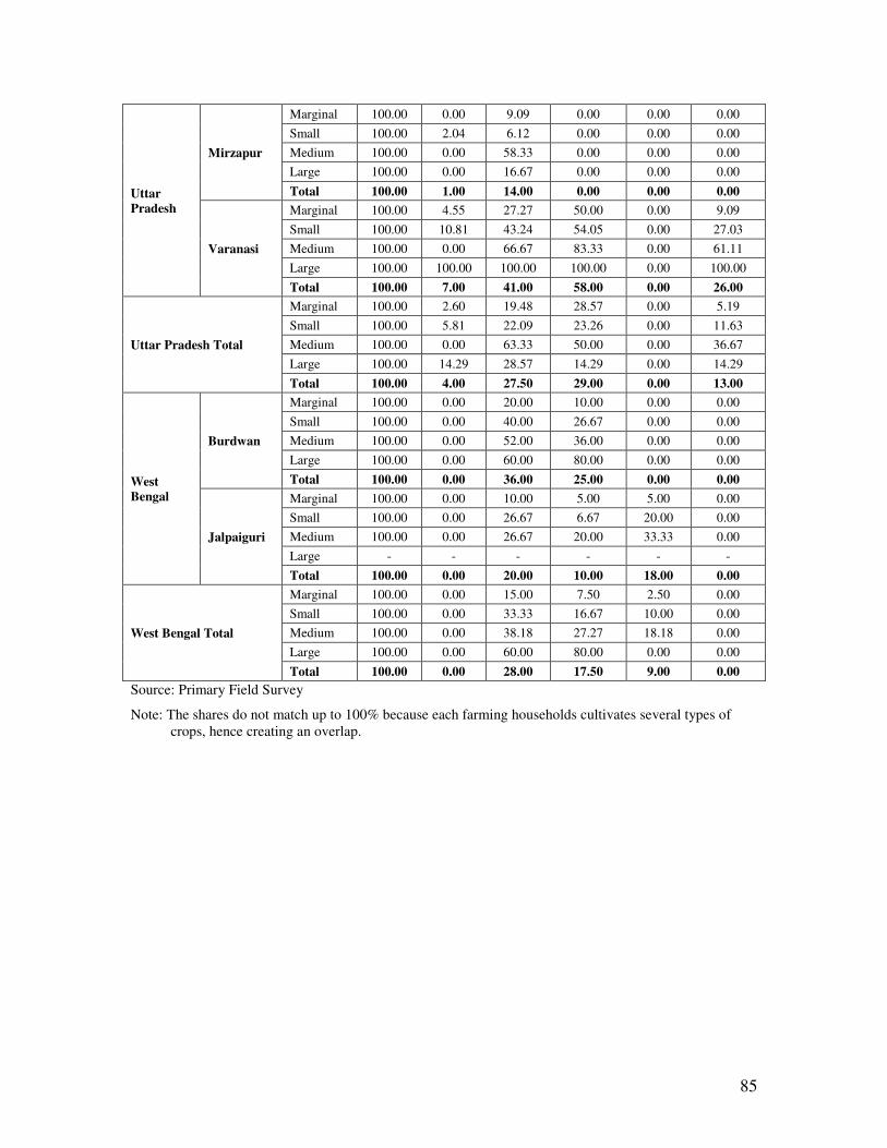
85
Uttar Pradesh
Mirzapur
Marginal 100.00 0.00 9.09 0.00 0.00 0.00
Small 100.00 2.04 6.12 0.00 0.00 0.00
Medium 100.00 0.00 58.33 0.00 0.00 0.00
Large 100.00 0.00 16.67 0.00 0.00 0.00
Total 100.00 1.00 14.00 0.00 0.00 0.00
Varanasi
Marginal 100.00 4.55 27.27 50.00 0.00 9.09
Small 100.00 10.81 43.24 54.05 0.00 27.03
Medium 100.00 0.00 66.67 83.33 0.00 61.11
Large 100.00 100.00 100.00 100.00 0.00 100.00
Total 100.00 7.00 41.00 58.00 0.00 26.00
Uttar Pradesh Total
Marginal 100.00 2.60 19.48 28.57 0.00 5.19
Small 100.00 5.81 22.09 23.26 0.00 11.63
Medium 100.00 0.00 63.33 50.00 0.00 36.67
Large 100.00 14.29 28.57 14.29 0.00 14.29
Total 100.00 4.00 27.50 29.00 0.00 13.00
West Bengal
Burdwan
Marginal 100.00 0.00 20.00 10.00 0.00 0.00
Small 100.00 0.00 40.00 26.67 0.00 0.00
Medium 100.00 0.00 52.00 36.00 0.00 0.00
Large 100.00 0.00 60.00 80.00 0.00 0.00
Total 100.00 0.00 36.00 25.00 0.00 0.00
Jalpaiguri
Marginal 100.00 0.00 10.00 5.00 5.00 0.00
Small 100.00 0.00 26.67 6.67 20.00 0.00
Medium 100.00 0.00 26.67 20.00 33.33 0.00
Large - - - - - -
Total 100.00 0.00 20.00 10.00 18.00 0.00
West Bengal Total
Marginal 100.00 0.00 15.00 7.50 2.50 0.00
Small 100.00 0.00 33.33 16.67 10.00 0.00
Medium 100.00 0.00 38.18 27.27 18.18 0.00
Large 100.00 0.00 60.00 80.00 0.00 0.00
Total 100.00 0.00 28.00 17.50 9.00 0.00
Source: Primary Field Survey
Note: The shares do not match up to 100% because each farming households cultivates several types of
crops, hence creating an overlap.
86
Cropping Pattern
Cropping pattern for each farm size category in all sample villages of the selected
districts in the four states is presented in Table 3.2. In the sample villages of Uttar
Pradesh, highest proportion of area was devoted to paddy (37.42%) followed closely by
Wheat (35.24%). Both the selected districts in Uttar Pradesh followed similar cropping
patterns except that cultivation of vegetables was seen only in Varanasi district. In the
selected districts of West Bengal, paddy occupied the largest proportion of GCA
(83.42%) followed by mustard (8.60%), jute (2.65%) and vegetables (2.31%). Jalpaiguri
followed the same pattern but in Burdwan, cultivation of jute was not reported. In the
selected districts of Bihar, paddy (36.84%) followed by wheat (19.88%) and khesari
(grass pea) (12.44%) occupied the largest proportion of area. Here the developed Rohtas
districts followed a similar cropping pattern, while in the underdeveloped district of
Kishanganj, paddy and wheat was followed by mustard (9.64%). In the selected districts
of Jharkhand, paddy occupied the largest proportion of area (39.85%), followed by maize
(17.11%), wheat (13.64%). Both the districts showed a similar cropping pattern. In the
selected districts of Orissa, paddy occupied the largest proportion of area (64.09%),
followed by mustard (16.78%). The developed district of Bhadrak showed a similar
trend, while in the under developed district of Kandhamal, highest proportion of area was
under paddy (74.60%) followed by vegetables (7.60%) and maize (7.52%).
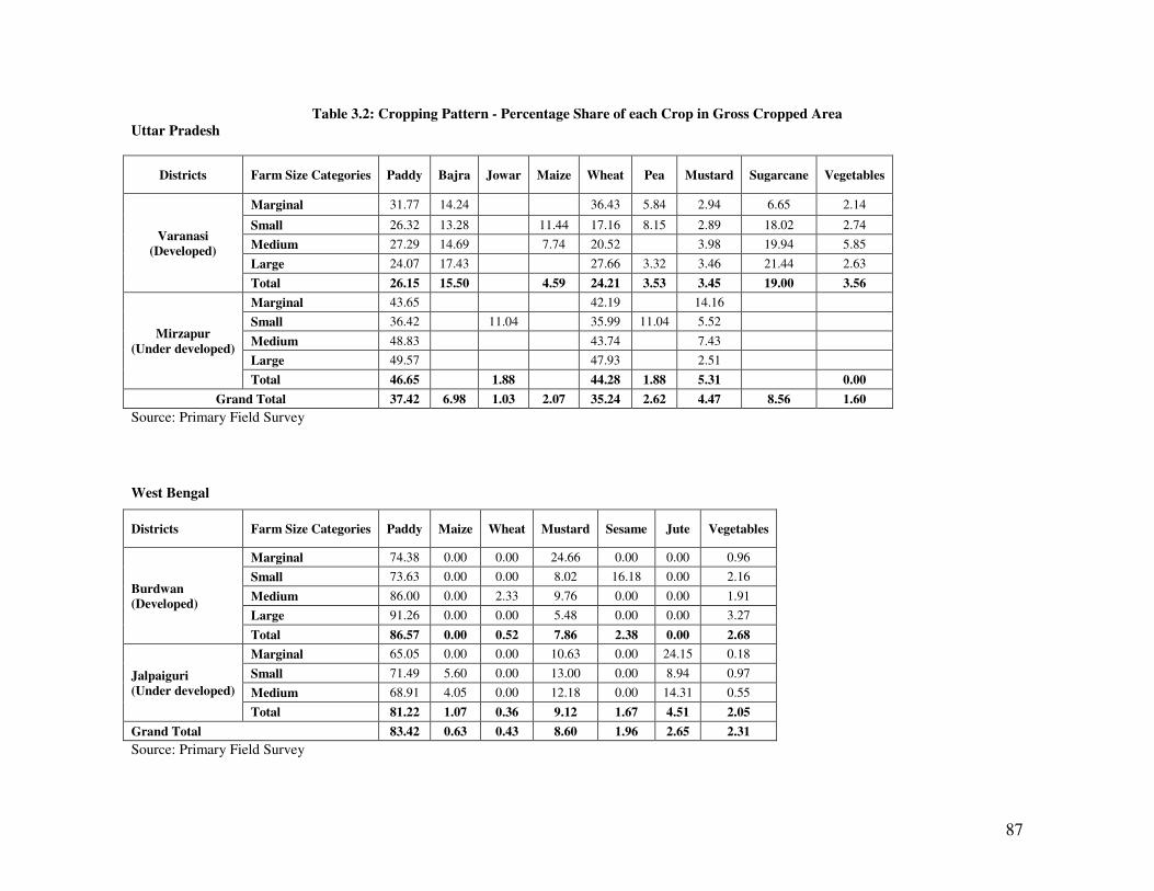
87
Table 3.2: Cropping Pattern - Percentage Share of each Crop in Gross Cropped Area
Uttar Pradesh
Districts Farm Size Categories Paddy Bajra Jowar Maize Wheat Pea Mustard Sugarcane Vegetables
Varanasi (Developed)
Marginal 31.77 14.24 36.43 5.84 2.94 6.65 2.14
Small 26.32 13.28 11.44 17.16 8.15 2.89 18.02 2.74
Medium 27.29 14.69 7.74 20.52 3.98 19.94 5.85
Large 24.07 17.43 27.66 3.32 3.46 21.44 2.63
Total 26.15 15.50 4.59 24.21 3.53 3.45 19.00 3.56
Mirzapur
(Under developed)
Marginal 43.65 42.19 14.16
Small 36.42 11.04 35.99 11.04 5.52
Medium 48.83 43.74 7.43
Large 49.57 47.93 2.51
Total 46.65 1.88 44.28 1.88 5.31 0.00
Grand Total 37.42 6.98 1.03 2.07 35.24 2.62 4.47 8.56 1.60
Source: Primary Field Survey
West Bengal
Districts Farm Size Categories Paddy Maize Wheat Mustard Sesame Jute Vegetables
Burdwan (Developed)
Marginal 74.38 0.00 0.00 24.66 0.00 0.00 0.96
Small 73.63 0.00 0.00 8.02 16.18 0.00 2.16
Medium 86.00 0.00 2.33 9.76 0.00 0.00 1.91
Large 91.26 0.00 0.00 5.48 0.00 0.00 3.27
Total 86.57 0.00 0.52 7.86 2.38 0.00 2.68
Jalpaiguri (Under developed)
Marginal 65.05 0.00 0.00 10.63 0.00 24.15 0.18
Small 71.49 5.60 0.00 13.00 0.00 8.94 0.97
Medium 68.91 4.05 0.00 12.18 0.00 14.31 0.55
Total 81.22 1.07 0.36 9.12 1.67 4.51 2.05
Grand Total 83.42 0.63 0.43 8.60 1.96 2.65 2.31
Source: Primary Field Survey
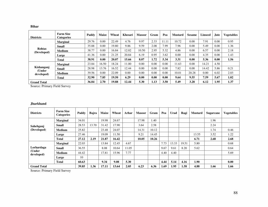
88
Bihar
Districts Farm Size Categories
Paddy Maize Wheat Khesari Masoor Gram Pea Mustard Sesame Linseed Jute Vegetables
Rohtas
(Developed)
Marginal 29.76 0.00 22.49 4.76 9.97 2.33 11.11 10.72 0.00 7.91 0.00 0.95
Small 35.88 0.00 19.80 9.86 9.59 2.08 7.99 7.96 0.00 5.49 0.00 1.36
Medium 38.77 0.00 16.84 12.02 10.50 2.95 5.32 4.86 0.00 6.57 0.00 2.18
Large 41.36 0.00 21.25 20.84 6.19 0.95 3.62 0.00 0.00 4.35 0.00 1.43
Total 38.91 0.00 20.07 15.66 8.07 1.72 5.34 3.31 0.00 5.36 0.00 1.56
Kishanganj (Under
developed)
Marginal 23.84 16.50 18.24 11.00 0.00 0.00 0.00 11.63 0.00 14.21 4.58
Small 28.98 13.76 16.52 12.44 0.00 0.00 0.00 7.82 0.00 14.42 5.86 0.21
Medium 39.56 0.00 22.09 0.00 0.00 0.00 0.00 10.01 20.28 0.00 6.02 2.03
Total 32.90 7.85 19.50 6.29 0.00 0.00 0.00 9.64 9.55 7.59 5.67 1.02
Grand Total 36.84 2.70 19.88 12.44 5.30 1.13 3.50 5.49 3.28 6.12 1.95 1.37
Source: Primary Field Survey
Jharkhand
Districts Farm Size Categories
Paddy Bajra Maize Wheat Arhar Masoor Gram Pea Urad Ragi Mustard Sugarcane Vegetables
Sahebganj (Developed)
Marginal 34.01 19.98 24.67 17.98 1.40 1.96
Small 28.53 13.70 31.42 17.90 3.64 2.58 2.24
Medium 25.82 23.48 24.07 14.31 10.12 1.74 0.46
Large 27.46 19.09 11.50 9.21 14.45 13.55 3.52 1.22
Total 27.12 2.19 21.87 16.42 10.05 10.26 6.71 2.68 2.68
Lorhardaga (Under developed)
Marginal 22.03 13.84 12.45 4.67 7.73 13.33 19.51 5.80 0.68
Small 36.55 8.08 10.64 11.05 9.67 9.61 8.20 5.62 0.64
Medium 44.42 17.81 15.96 7.77 4.40 4.40 5.69
Large 10
Total 60.63 9.34 9.08 5.30 4.44 5.14 4.16 1.90 0.00
Grand Total 39.85 1.36 17.11 13.64 2.05 6.23 6.36 1.69 1.95 1.58 4.88 1.66 1.66
Source: Primary Field Survey
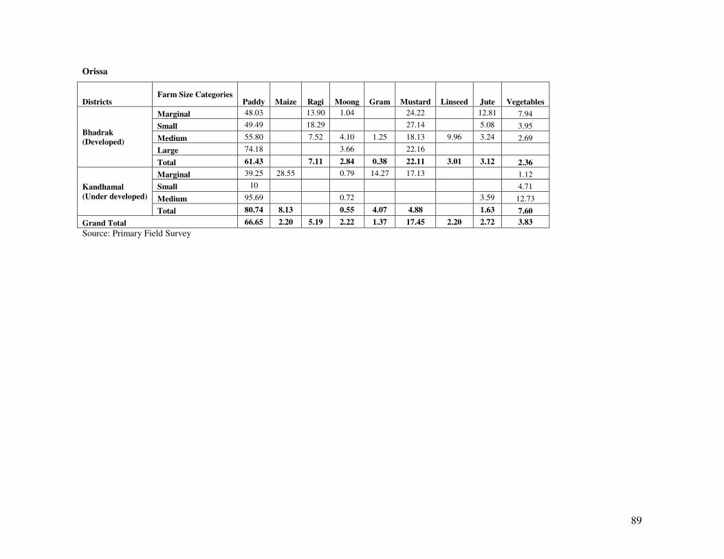
89
Orissa
Districts Farm Size Categories
Paddy Maize Ragi Moong Gram Mustard Linseed Jute Vegetables
Bhadrak (Developed)
Marginal 48.03 13.90 1.04 24.22 12.81 7.94
Small 49.49 18.29 27.14 5.08 3.95
Medium 55.80 7.52 4.10 1.25 18.13 9.96 3.24 2.69
Large 74.18 3.66 22.16
Total 61.43 7.11 2.84 0.38 22.11 3.01 3.12 2.36
Kandhamal
(Under developed)
Marginal 39.25 28.55 0.79 14.27 17.13 1.12
Small 10 4.71
Medium 95.69 0.72 3.59 12.73
Total 80.74 8.13 0.55 4.07 4.88 1.63 7.60
Grand Total 66.65 2.20 5.19 2.22 1.37 17.45 2.20 2.72 3.83
Source: Primary Field Survey
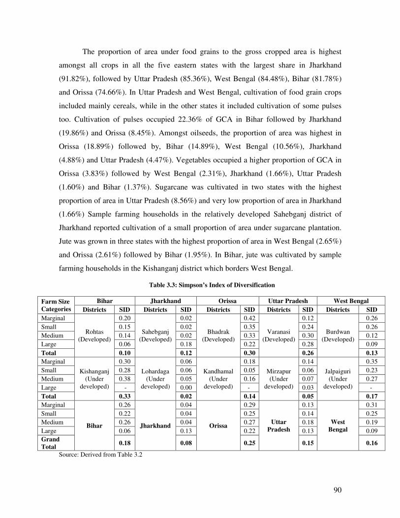
90
The proportion of area under food grains to the gross cropped area is highest
amongst all crops in all the five eastern states with the largest share in Jharkhand
(91.82%), followed by Uttar Pradesh (85.36%), West Bengal (84.48%), Bihar (81.78%)
and Orissa (74.66%). In Uttar Pradesh and West Bengal, cultivation of food grain crops
included mainly cereals, while in the other states it included cultivation of some pulses
too. Cultivation of pulses occupied 22.36% of GCA in Bihar followed by Jharkhand
(19.86%) and Orissa (8.45%). Amongst oilseeds, the proportion of area was highest in
Orissa (18.89%) followed by, Bihar (14.89%), West Bengal (10.56%), Jharkhand
(4.88%) and Uttar Pradesh (4.47%). Vegetables occupied a higher proportion of GCA in
Orissa (3.83%) followed by West Bengal (2.31%), Jharkhand (1.66%), Uttar Pradesh
(1.60%) and Bihar (1.37%). Sugarcane was cultivated in two states with the highest
proportion of area in Uttar Pradesh (8.56%) and very low proportion of area in Jharkhand
(1.66%) Sample farming households in the relatively developed Sahebganj district of
Jharkhand reported cultivation of a small proportion of area under sugarcane plantation.
Jute was grown in three states with the highest proportion of area in West Bengal (2.65%)
and Orissa (2.61%) followed by Bihar (1.95%). In Bihar, jute was cultivated by sample
farming households in the Kishanganj district which borders West Bengal.
Table 3.3: Simpson’s Index of Diversification
Farm Size Categories
Bihar Jharkhand Orissa Uttar Pradesh West Bengal
Districts SID Districts SID Districts SID Districts SID Districts SID
Marginal
Rohtas
(Developed)
0.20
Sahebganj
(Developed)
0.02
Bhadrak
(Developed)
0.42
Varanasi
(Developed)
0.12
Burdwan
(Developed)
0.26
Small 0.15 0.02 0.35 0.24 0.26
Medium 0.14 0.02 0.33 0.30 0.12
Large 0.06 0.18 0.22 0.28 0.09
Total 0.10 0.12 0.30 0.26 0.13
Marginal
Kishanganj
(Under
developed)
0.30
Lohardaga
(Under
developed)
0.06
Kandhamal
(Under
developed)
0.18
Mirzapur
(Under
developed)
0.14
Jalpaiguri
(Under
developed)
0.35
Small 0.28 0.06 0.05 0.06 0.23
Medium 0.38 0.05 0.16 0.07 0.27
Large - 0.00 - 0.03 -
Total 0.33 0.02 0.14 0.05 0.17
Marginal
Bihar
0.26
Jharkhand
0.04
Orissa
0.29
Uttar
Pradesh
0.13
West
Bengal
0.31
Small 0.22 0.04 0.25 0.14 0.25
Medium 0.26 0.04 0.27 0.18 0.19
Large 0.06 0.13 0.22 0.13 0.09
Grand
Total 0.18 0.08 0.25 0.15 0.16
Source: Derived from Table 3.2
91
The Simpson’s Index of Diversification (SID) (Table 3.3) is the highest in Orissa
(0.25) followed by Bihar (0.18), West Bengal (0.16), Uttar Pradesh (0.15), and Jharkhand
(0.08). In the states of Orissa, Bihar, West Bengal and Jharkhand the crop diversification
away from food grains is mainly towards oilseeds while in Uttar Pradesh it is mainly
towards sugarcane. Some diversification towards cultivation of vegetables was observed
mainly in the states of Orissa and West Bengal (Table 3.2). It is also seen from the above
table that developed districts show greater crop diversification away from food grains
towards non-food grain crops compared to under developed districts except for
Kishanganj in Bihar and Jalpaiguri in West Bengal which showed diversification towards
oilseeds and jute.
Across farm size classes it was also seen from the above index that in the state of
Jharkhand where crop diversification away from food grains is the least, small and
marginal farmers show lesser crop diversification compared to large farmers in the
developed Sahebganj district. While in the relatively under developed Lohardaga district
small and marginal farmers showed comparatively greater diversification away from food
grains compared to medium and large farmers. In the state of Uttar Pradesh, small and
marginal farmers show lesser crop diversification away from food grains compared to
large and medium farmers in the developed Varanasi district. While in the relatively
under developed district of Mirzapur, marginal farmers show greater crop diversification
compared to small, medium and large farmers. In the state of West Bengal, small and
marginal farmers show greater crop diversification away from food grains compared to
medium and large farmers in the developed Burdwan district while in the relatively under
developed Jalpaiguri district marginal farmers show the highest diversification followed
by medium and small farmers. In the developed Rohtas district of Bihar, small and
marginal farmers show greater crop diversification away from food grains compared to
medium and large farmers, while in the relatively under developed district of Kishanganj,
medium farmers showed a slightly greater diversification away from food grains
compared to small and marginal farmers. In the state of Orissa, where crop diversification
away from food grains is the highest, small and marginal farmers show greater crop
diversification compared to large farmers in the developed Bhadrak district, while in the
92
relatively underdeveloped Khandamal district, marginal farmers showed highest crop
diversification followed by medium farmers and then small farmers.
Hence overall it is seen that in the selected states where crop diversification away
from food grains is the least namely Jharkhand, small and marginal farmers are
diversifying less compared to the other categories. In Uttar Pradesh, diversification by
medium farmers is the highest followed by small, marginal and large farmers. In Bihar
marginal and medium farmers are diversifying the most followed closely by small
farmers and diversification by large farmers is the least. In Orissa marginal farmers are
diversifying the most followed closely by medium, small and large farmers. In West
Bengal highest diversification is by small and marginal farmers. Hence, overall it is seen
that small and marginal farmers are diversifying more within the crop sector.
From the Table 3.2 it is seen that in the state of Bihar, marginal, small and
medium farmers are mainly diversifying away from food grains by allocating higher
proportion of area or diversifying more towards oilseeds (mustard and linseed) followed
by jute and then vegetables, while large farmers are diversifying towards oilseeds
(sesame) and vegetables. The area devoted by marginal, small and medium farmers
towards oilseeds cultivation is 22.7%, 18% and 21% respectively. Towards jute, their
proportional area allocation is 2.59%, 3.02% and 3.07% respectively and for vegetables it
is 0.41%, 0.76% and 2.10% respectively. The area devoted by large farmers towards
oilseeds cultivation is 4.35% and for vegetables it is 1.43% respectively. In Orissa, small
and marginal farmers are mainly diversifying towards oilseeds (mustard and linseed)
followed closely by jute and vegetables, while large farmers are diversifying only
towards oilseeds (mustard). The area devoted by marginal and small farmers towards
oilseeds cultivation is 19.49% and 17.39% respectively. Towards jute, their proportional
area allocation is 5.62% and 3.26% respectively and for vegetables it is 4.37% and 4.21%
respectively. The area devoted by large farmers towards oilseeds cultivation is 22.16%.
In West Bengal marginal, small and medium farmers are diversifying mainly towards
oilseeds (mustard and sesame) and jute followed by vegetables while large farmers are
diversifying only towards oilseeds (mustard) and vegetables. The area devoted by
marginal, small and medium farmers towards oilseeds cultivation is 15.87%, 19.41% and
10.98% respectively. Towards jute, their proportional area allocation is 15.12%, 3.82%
93
and & 7.22% respectively and for vegetables it is 0.47%, 1.65% and 1.23% respectively.
The area devoted by large farmers towards oilseeds cultivation is 5.48% and for
vegetables it is 3.27% respectively. In Uttar Pradesh, marginal farmers are mainly
diversifying towards mustard (8.82%) followed by sugarcane (3.17%) and vegetables
(1.02%). Small farmers are devoting a higher proportion of area towards sugarcane
(8.85%) followed by mustard (4.23%) and vegetables (1.35%). Medium farmers are also
devoting a higher proportion of area towards sugarcane (9.33%) followed by mustard
(5.81%) and vegetables (2.74%). Large farmers are diversifying mainly towards
sugarcane (8.96%) followed by mustard (2.91%) and vegetables (1.10%). Jharkhand is
the only state where large farmers are diversifying the most and they are mainly
diversifying towards mustard (9.42%) followed by sugarcane (2.45%) and vegetables
(0.85%). Marginal and small farmers taken together are also diversifying into mustard
(5.56%) followed by sugarcane (2.17%) and vegetables (0.64%). Medium farmers are
mainly diversifying into vegetables (2.77%) and then sugarcane (0.97%).
So, horizontal diversification of small and marginal farms towards high value
crops is seen to be more than large farms in the study regions. In case of proportion of
area devoted to vegetable crops, a positive relationship is observed, but this relationship
is not significant because it is also observed that the proportion area devoted to
vegetables by large farmers is less compared to marginal, small and medium farming
categories. Cultivation of vegetables is labour intensive and small and marginal farmers
have family labour at their disposal which large farmers don’t, resulting in constraints
imposed by availability of family labour in expanding area under vegetables for large
farmers.
This field study shows an in inverse relationship between farm size and high
value crop diversification (oilseeds, sugarcane, jute and vegetables). The reasons for this
is that, since high value crops gives better yields and earlier returns compared to food
grains, small and marginal farmers try to maximize their returns from their small holdings
by allocating more acreages to these high value crops whereas large farmers tend to
hedge their bets by devoting more area towards food grains and also diversifying more
within the allied sectors like livestock and fisheries that shall be seen later in this chapter.
94
Crop Yields
Yields of crops surveyed in the sample villages of the study region are given in
table 3.4. It is seen that amongst all crops per hectare yields for vegetables were highest
in Uttar Pradesh 137.27 Qtl/Hec, followed by Jharkhand (98.85 Qtl/Hec), West Bengal
(82.45 Qtl/Hec), Orissa (60.88 Qtl/Hec) and Bihar (17.03 Qtl/Hec). Vegetable yields
were low in Bihar and Orissa compared to the former states because these states mostly
cultivated green leafy vegetables whose yields are usually lower than onions and potatoes
which are mostly cultivated in the former states. The yield levels of sugarcane crop were
also high i.e., 68.50 Qtl/Hec in Uttar Pradesh and 56.25 Qtl/Hec in Jharkhand (Table 3.4).
Amongst the five selected states paddy was cultivated in all of them and the highest
yields were seen in Orissa (22.25 Qtl/Hec) and Uttar Pradesh (22.20 Qtl/Hec) followed
by Bihar (16.86 Qtl/Hec), West Bengal (13.39 Qtl/Hec) and Jharkhand (12.75 Qtl/Hec).
Wheat showed highest yields in Bihar (11.97) followed by UP (8.21 Qtl/Hec), Jharkhand
(7 Qtl/Hec) and West Bengal (5.33 Qtl/Hec). Maize was cultivated in all the states with
the highest yields reporting from Bihar (19.24 Qtl/Hec), UP (14.35 Qtl/Hec), WB (12.74
Qtl/Hec), Jharkhand (12 Qtl/Hec) and Orissa (3 Qtl/Hec). Bajra was cultivated only in
two states Jharkhand (15 Qtl/Hec) and Uttar Pradesh (7.31 Qtl/Hec). Jowar was
cultivated only in UP with yields of 8 Qtls/Hec. Ragi was cultivated only in Jharkhand
with yields of 2.85 Qtls/Hec. Pea was cultivated in three states with highest yields in
Bihar (4.22 Qtl/Hec) followed by Uttar Pradesh (3.65 Qtl/Hec) and Jharkhand (3.17
Qtl/Hec). Mustard was cultivated in all the states with highest yields in Jharkhand (7.44
Qtl/Hec) followed by West Bengal (5.30 Qtl/Hec), Uttar Pradesh (5.07 Qtl/Hec), Bihar
(3.32 Qtl/Hec) and Orissa (1.17 Qtl/Hec). Khesari (grass pea) was grown only in Bihar
with yield of 4.02 Qtls/Hec. Masoor (Lentil) was cultivated only in Bihar and Jharkhand
with yields of 3.51 and 2.78 Qtls/Hec respectively. Gram was cultivated in Bihar,
Jharkhand and Orissa with very low yields of less than 1 Qtl/Hec in all three states. Arhar
(reg gram) and urad (black gram) was cultivated only in Jharkhand with yields of 2.83
and 2.28 Qtls/Hec respectively. Moong (green gram) was cultivated only in Orissa with
yields of 1.16 Qtls/Hec. Sesame was cultivated in Bihar and West Bengal with yields of
3.50 and 4.50 Qtls/Hec respectively. Linseed (tisi) was cultivated in Bihar and Orissa
with yields of 1.86 and 3.00 Qtls/Hec respectively. Jute was cultivated in three states with
95
highest yields in West Bengal (11.99 Qtl/Hec), Orissa (10.74 Qtl/Hec) and Bihar (8.63
Qtl/Hec).
In all the five states it is seen that the yields from high value crops (oilseeds,
sugarcane, jute and vegetables) is higher than food grain crops. An exception to this was
the relatively under developed districts of Kishanganj in Bihar and the Mirzapur in Uttar
Pradesh where yields from food grains were greater than high value crops. Among all the
high value crops which were seen in the selected sample regions, the yields of vegetables
were the highest.
Across farm size categories it is seen that in the state of Uttar Pradesh, all farm
sizes show a positive relationship with the cultivation of food grains (Table 3.4). In case
of high value crops (oilseeds, sugarcane and vegetables) the yields in the district of
Varanasi are high for marginal followed by small and large farmers. The yields of
medium farmers are slightly less. The yields of oilseeds (mustard) show a positive
relationship across farm sizes while for sugarcane the yields are high for marginal
farmers followed by large farmers. In the relatively under developed Mirzapur districts
all categories of farmers are cultivating only oilseeds whose yields show a positive
relation with farm size.
In Bihar, all categories of farmers show a positive relationship with the cultivation
of food grains especially in the developed Rohtas district. In the relatively under
developed Kishanganj district, marginal and medium farmers show high food grain yields
while small farmers show slightly lower yields. In case of high value crops, the yields in
the district of Rohtas are high for large followed by marginal, medium and small farmers,
while in Kishanganj it shows a positive relation. Among high value crops, oilseeds
(mustard, sesame and linseed) show a positive relationship with farm sizes in both
districts of Bihar. jute yields in Kishanganj district are highest for small followed by
marginal and medium farmers. Vegetable yields in Rohtas district are highest for
marginal followed by large, medium and small farmers.
In Jharkhand, all categories of farmers show a positive relationship with the
cultivation of food grains in both Sahebganj and Lohardaga districts. The farm size and
productivity relationship of high value crops (mustard, vegetables and sugarcane) is also
positive in the sample villages of both districts.
96
In Orissa, all categories of farmers show a positive relationship with the
cultivation of food grains in the sample villages of both Bhadrak and Khandamal
districts. The farm size and productivity relationship of high value crops (mustard,
linseed, jute and vegetables) is also positive in the sample villages of both districts.
In West Bengal, all categories of farmers show a positive relationship with the
cultivation of food grains in the sample villages of both Burdwan and Jalpaiguri districts.
The farm size and productivity relationship of high value crops (mustard, sesame, jute
and vegetables) is also positive in the sample villages of both districts.
In all the selected five states, the developed districts showed higher yield levels
for most crops than the underdeveloped districts. It is also noticed that most crop yields
showed a positive relation with farm size in all the five states surveyed. Further, it is also
seen that crop diversification towards high value crops, mainly vegetables and sugarcane
suits the need of farmers especially small and marginal holders as the yield levels of these
crops are much higher compared to other crops and it was also reported by farmers that
the returns especially from vegetables were more regular and earlier compared to food
grains.
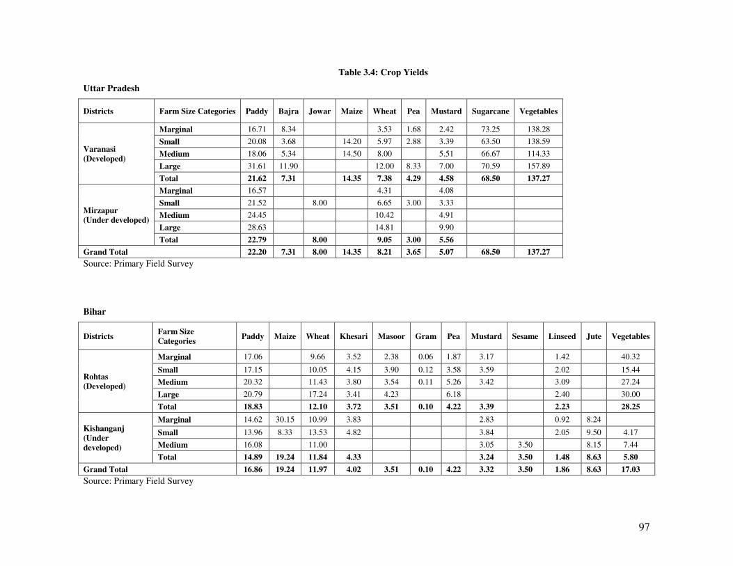
97
Table 3.4: Crop Yields
Uttar Pradesh
Districts Farm Size Categories Paddy Bajra Jowar Maize Wheat Pea Mustard Sugarcane Vegetables
Varanasi (Developed)
Marginal 16.71 8.34 3.53 1.68 2.42 73.25 138.28
Small 20.08 3.68 14.20 5.97 2.88 3.39 63.50 138.59
Medium 18.06 5.34 14.50 8.00 5.51 66.67 114.33
Large 31.61 11.90 12.00 8.33 7.00 70.59 157.89
Total 21.62 7.31 14.35 7.38 4.29 4.58 68.50 137.27
Mirzapur (Under developed)
Marginal 16.57 4.31 4.08
Small 21.52 8.00 6.65 3.00 3.33
Medium 24.45 10.42 4.91
Large 28.63 14.81 9.90
Total 22.79 8.00 9.05 3.00 5.56
Grand Total 22.20 7.31 8.00 14.35 8.21 3.65 5.07 68.50 137.27
Source: Primary Field Survey
Bihar
Districts Farm Size Categories
Paddy Maize Wheat Khesari Masoor Gram Pea Mustard Sesame Linseed Jute Vegetables
Rohtas (Developed)
Marginal 17.06 9.66 3.52 2.38 0.06 1.87 3.17 1.42 40.32
Small 17.15 10.05 4.15 3.90 0.12 3.58 3.59 2.02 15.44
Medium 20.32 11.43 3.80 3.54 0.11 5.26 3.42 3.09 27.24
Large 20.79 17.24 3.41 4.23 6.18 2.40 30.00
Total 18.83 12.10 3.72 3.51 0.10 4.22 3.39 2.23 28.25
Kishanganj (Under
developed)
Marginal 14.62 30.15 10.99 3.83 2.83 0.92 8.24
Small 13.96 8.33 13.53 4.82 3.84 2.05 9.50 4.17
Medium 16.08 11.00 3.05 3.50 8.15 7.44
Total 14.89 19.24 11.84 4.33 3.24 3.50 1.48 8.63 5.80
Grand Total 16.86 19.24 11.97 4.02 3.51 0.10 4.22 3.32 3.50 1.86 8.63 17.03
Source: Primary Field Survey

98
Jharkhand
Districts Farm Size Categories
Paddy Bajra Maize Wheat Arhar Masoor Gram Pea Urad Ragi Mustard Sugarcane Vegetables
Sahebganj
(Developed)
Marginal 6.05 15.41 2.88 1.83 0.01 50.00
Small 11.33 15.00 5.43 4.14 2.00 0.16 55.00
Medium 15.27 12.54 12.64 2.88 0.63 60.00 130.00
Large 20.11 15.43 16.07 4.41 0.40 9.26 60.00 160.00
Total 13.19 15.00 12.20 8.93 2.78 0.30 9.26 56.25 145.00
Lohardaga (Under developed)
Marginal 11.16 10.70 3.09 2.50 1.08 1.79 2.54 5.00 20.12
Small 9.71 9.71 4.83 3.00 3.93 1.54 3.17 6.25 42.50
Medium 13.93 15.00 7.25 3.00 4.50 3.50 95.47
Large 14.40
Total 12.30 11.80 5.06 2.83 3.17 2.28 2.85 5.63 52.70
Grand Total 12.75 15.00 12.00 7.00 2.83 2.78 0.30 3.17 2.28 2.85 7.44 56.25 98.85
Source: Primary Field Survey
Orissa
Districts Farm Size Categories Paddy Maize Moong Gram Ragi Mustard Linseed Jute Vegetables
Bhadrak (Developed)
Marginal 18.18 0.85 0.04 0.83 6.85 72.14
Small 21.02 1.03 0.94 7.06 74.60
Medium 25.36 1.60 0.86 1.20 1.60 3.00 11.54 74.59
Large 26.90 1.00 2.00
Total 22.87 1.16 0.63 1.20 1.34 3.00 8.48 73.78
Kandhamal (Under developed)
Marginal 19.85 3.00 0.02 3.00 1.00 29.19
Small 23.07 49.03
Medium 21.97 0.08 13.00 65.76
Total 21.63 3.00 0.05 3.00 1.00 13.00 47.99
Grand Total 22.25 3.00 1.16 0.34 2.10 1.17 3.00 10.74 60.88
Source: Primary Field Survey
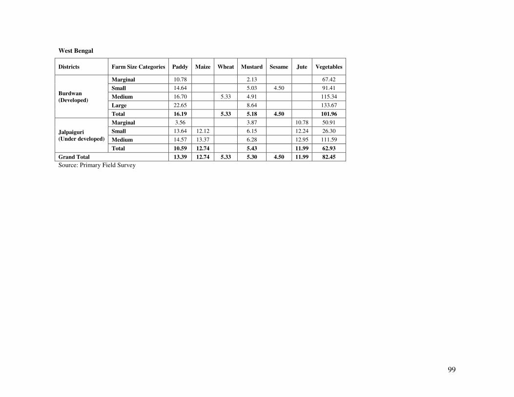
99
West Bengal
Districts Farm Size Categories Paddy Maize Wheat Mustard Sesame Jute Vegetables
Burdwan
(Developed)
Marginal 10.78 2.13 67.42
Small 14.64 5.03 4.50 91.41
Medium 16.70 5.33 4.91 115.34
Large 22.65 8.64 133.67
Total 16.19 5.33 5.18 4.50 101.96
Jalpaiguri (Under developed)
Marginal 3.56 3.87 10.78 50.91
Small 13.64 12.12 6.15 12.24 26.30
Medium 14.57 13.37 6.28 12.95 111.59
Total 10.59 12.74 5.43 11.99 62.93
Grand Total 13.39 12.74 5.33 5.30 4.50 11.99 82.45
Source: Primary Field Survey
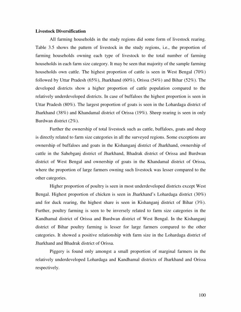
100
Livestock Diversification
All farming households in the study regions did some form of livestock rearing.
Table 3.5 shows the pattern of livestock in the study regions, i.e., the proportion of
farming households owning each type of livestock to the total number of farming
households in each farm size category. It may be seen that majority of the sample farming
households own cattle. The highest proportion of cattle is seen in West Bengal (70%)
followed by Uttar Pradesh (65%), Jharkhand (60%), Orissa (54%) and Bihar (52%). The
developed districts show a higher proportion of cattle population compared to the
relatively underdeveloped districts. In case of buffaloes the highest proportion is seen in
Uttar Pradesh (80%). The largest proportion of goats is seen in the Lohardaga district of
Jharkhand (38%) and Khandamal district of Orissa (19%). Sheep rearing is seen in only
Burdwan district (2%).
Further the ownership of total livestock such as cattle, buffaloes, goats and sheep
is directly related to farm size categories in all the surveyed regions. Some exceptions are
ownership of buffaloes and goats in the Kishanganj district of Jharkhand, ownership of
cattle in the Sahebganj district of Jharkhand, Bhadrak district of Orissa and Burdwan
district of West Bengal and ownership of goats in the Khandamal district of Orissa,
where the proportion of large farmers owning such livestock was lesser compared to the
other categories.
Higher proportion of poultry is seen in most underdeveloped districts except West
Bengal. Highest proportion of chicken is seen in Jharkhand’s Lohardaga district (30%)
and for duck rearing, the highest share is seen in Kishanganj district of Bihar (3%).
Further, poultry farming is seen to be inversely related to farm size categories in the
Kandhamal district of Orissa and Burdwan district of West Bengal. In the Kishanganj
district of Bihar poultry farming is lesser for large farmers compared to the other
categories. It showed a positive relationship with farm size in the Lohardaga district of
Jharkhand and Bhadrak district of Orissa.
Piggery is found only amongst a small proportion of marginal farmers in the
relatively underdeveloped Lohardaga and Kandhamal districts of Jharkhand and Orissa
respectively.
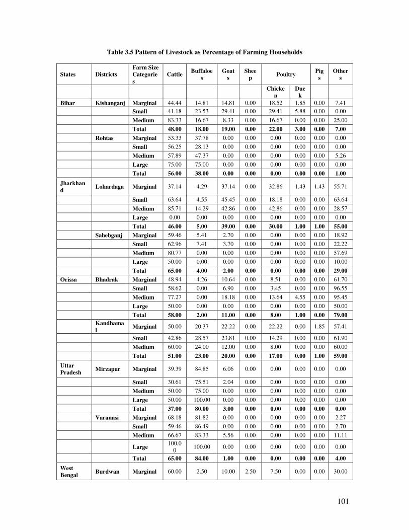
101
Table 3.5 Pattern of Livestock as Percentage of Farming Households
States Districts Farm Size Categories
Cattle Buffaloe
s Goat
s Shee
p Poultry
Pigs
Others
Chicke
n Duc
k
Bihar Kishanganj Marginal 44.44 14.81 14.81 0.00 18.52 1.85 0.00 7.41
Small 41.18 23.53 29.41 0.00 29.41 5.88 0.00 0.00
Medium 83.33 16.67 8.33 0.00 16.67 0.00 0.00 25.00
Total 48.00 18.00 19.00 0.00 22.00 3.00 0.00 7.00
Rohtas Marginal 53.33 37.78 0.00 0.00 0.00 0.00 0.00 0.00
Small 56.25 28.13 0.00 0.00 0.00 0.00 0.00 0.00
Medium 57.89 47.37 0.00 0.00 0.00 0.00 0.00 5.26
Large 75.00 75.00 0.00 0.00 0.00 0.00 0.00 0.00
Total 56.00 38.00 0.00 0.00 0.00 0.00 0.00 1.00
Jharkhand
Lohardaga Marginal 37.14 4.29 37.14 0.00 32.86 1.43 1.43 55.71
Small 63.64 4.55 45.45 0.00 18.18 0.00 0.00 63.64
Medium 85.71 14.29 42.86 0.00 42.86 0.00 0.00 28.57
Large 0.00 0.00 0.00 0.00 0.00 0.00 0.00 0.00
Total 46.00 5.00 39.00 0.00 30.00 1.00 1.00 55.00
Sahebganj Marginal 59.46 5.41 2.70 0.00 0.00 0.00 0.00 18.92
Small 62.96 7.41 3.70 0.00 0.00 0.00 0.00 22.22
Medium 80.77 0.00 0.00 0.00 0.00 0.00 0.00 57.69
Large 50.00 0.00 0.00 0.00 0.00 0.00 0.00 10.00
Total 65.00 4.00 2.00 0.00 0.00 0.00 0.00 29.00
Orissa Bhadrak Marginal 48.94 4.26 10.64 0.00 8.51 0.00 0.00 61.70
Small 58.62 0.00 6.90 0.00 3.45 0.00 0.00 96.55
Medium 77.27 0.00 18.18 0.00 13.64 4.55 0.00 95.45
Large 50.00 0.00 0.00 0.00 0.00 0.00 0.00 50.00
Total 58.00 2.00 11.00 0.00 8.00 1.00 0.00 79.00
Kandhamal
Marginal 50.00 20.37 22.22 0.00 22.22 0.00 1.85 57.41
Small 42.86 28.57 23.81 0.00 14.29 0.00 0.00 61.90
Medium 60.00 24.00 12.00 0.00 8.00 0.00 0.00 60.00
Total 51.00 23.00 20.00 0.00 17.00 0.00 1.00 59.00
Uttar Pradesh
Mirzapur Marginal 39.39 84.85 6.06 0.00 0.00 0.00 0.00 0.00
Small 30.61 75.51 2.04 0.00 0.00 0.00 0.00 0.00
Medium 50.00 75.00 0.00 0.00 0.00 0.00 0.00 0.00
Large 50.00 100.00 0.00 0.00 0.00 0.00 0.00 0.00
Total 37.00 80.00 3.00 0.00 0.00 0.00 0.00 0.00
Varanasi Marginal 68.18 81.82 0.00 0.00 0.00 0.00 0.00 2.27
Small 59.46 86.49 0.00 0.00 0.00 0.00 0.00 2.70
Medium 66.67 83.33 5.56 0.00 0.00 0.00 0.00 11.11
Large 100.0
0 100.00 0.00 0.00 0.00 0.00 0.00 0.00
Total 65.00 84.00 1.00 0.00 0.00 0.00 0.00 4.00
West Bengal
Burdwan Marginal 60.00 2.50 10.00 2.50 7.50 0.00 0.00 30.00
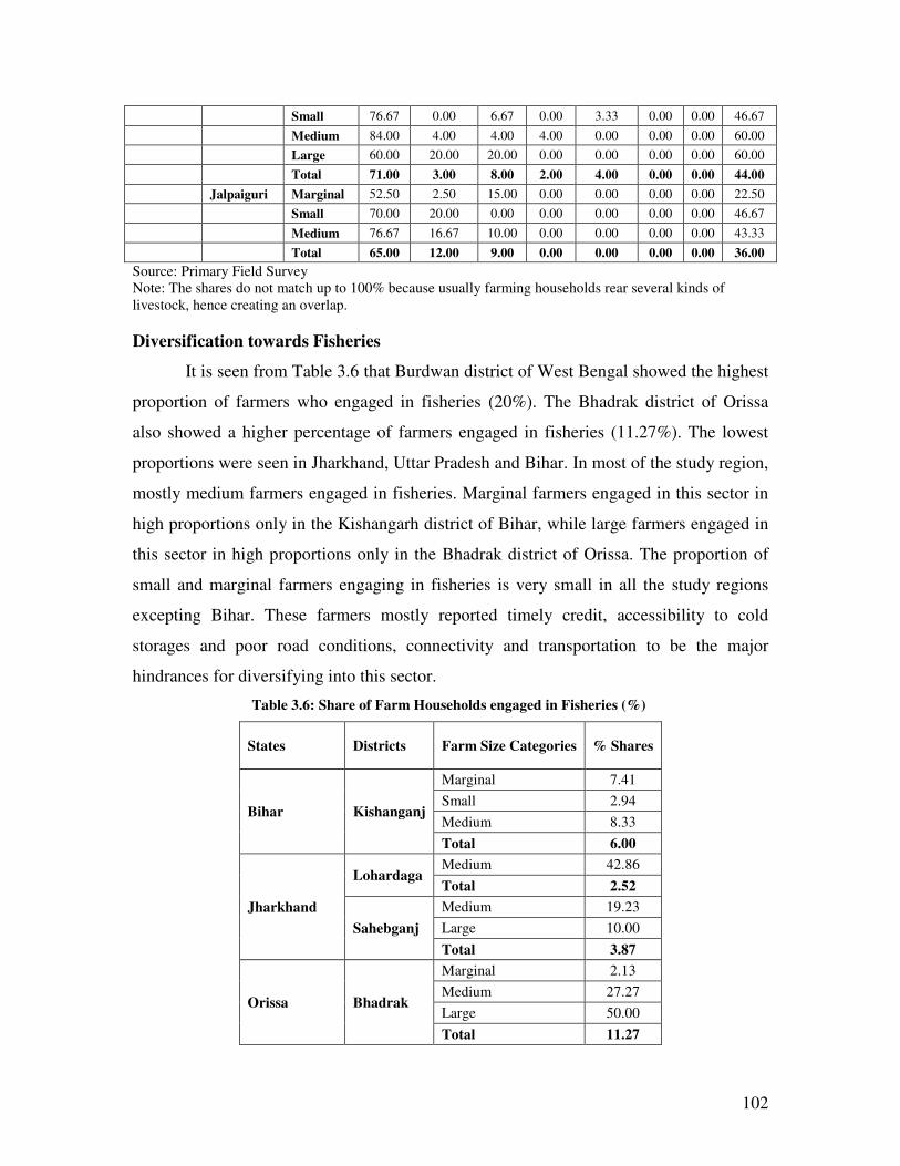
102
Small 76.67 0.00 6.67 0.00 3.33 0.00 0.00 46.67
Medium 84.00 4.00 4.00 4.00 0.00 0.00 0.00 60.00
Large 60.00 20.00 20.00 0.00 0.00 0.00 0.00 60.00
Total 71.00 3.00 8.00 2.00 4.00 0.00 0.00 44.00
Jalpaiguri Marginal 52.50 2.50 15.00 0.00 0.00 0.00 0.00 22.50
Small 70.00 20.00 0.00 0.00 0.00 0.00 0.00 46.67
Medium 76.67 16.67 10.00 0.00 0.00 0.00 0.00 43.33
Total 65.00 12.00 9.00 0.00 0.00 0.00 0.00 36.00
Source: Primary Field Survey
Note: The shares do not match up to 100% because usually farming households rear several kinds of
livestock, hence creating an overlap.
Diversification towards Fisheries
It is seen from Table 3.6 that Burdwan district of West Bengal showed the highest
proportion of farmers who engaged in fisheries (20%). The Bhadrak district of Orissa
also showed a higher percentage of farmers engaged in fisheries (11.27%). The lowest
proportions were seen in Jharkhand, Uttar Pradesh and Bihar. In most of the study region,
mostly medium farmers engaged in fisheries. Marginal farmers engaged in this sector in
high proportions only in the Kishangarh district of Bihar, while large farmers engaged in
this sector in high proportions only in the Bhadrak district of Orissa. The proportion of
small and marginal farmers engaging in fisheries is very small in all the study regions
excepting Bihar. These farmers mostly reported timely credit, accessibility to cold
storages and poor road conditions, connectivity and transportation to be the major
hindrances for diversifying into this sector.
Table 3.6: Share of Farm Households engaged in Fisheries (%)
States Districts Farm Size Categories % Shares
Bihar Kishanganj
Marginal 7.41
Small 2.94
Medium 8.33
Total 6.00
Jharkhand
Lohardaga Medium 42.86
Total 2.52
Sahebganj
Medium 19.23
Large 10.00
Total 3.87
Orissa Bhadrak
Marginal 2.13
Medium 27.27
Large 50.00
Total 11.27
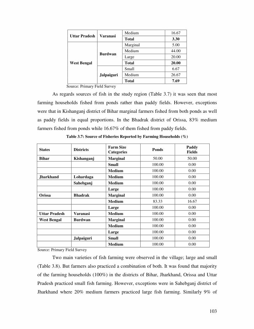
103
Uttar Pradesh Varanasi Medium 16.67
Total 3.30
West Bengal
Burdwan
Marginal 5.00
Medium 44.00
Large 20.00
Total 20.00
Jalpaiguri
Small 6.67
Medium 26.67
Total 7.69
Source: Primary Field Survey
As regards sources of fish in the study region (Table 3.7) it was seen that most
farming households fished from ponds rather than paddy fields. However, exceptions
were that in Kishanganj district of Bihar marginal farmers fished from both ponds as well
as paddy fields in equal proportions. In the Bhadrak district of Orissa, 83% medium
farmers fished from ponds while 16.67% of them fished from paddy fields.
Table 3.7: Source of Fisheries Reported by Farming Households (%)
States Districts Farm Size
Categories Ponds
Paddy
Fields
Bihar Kishanganj Marginal 50.00 50.00
Small 100.00 0.00
Medium 100.00 0.00
Jharkhand Lohardaga Medium 100.00 0.00
Sahebganj Medium 100.00 0.00
Large 100.00 0.00
Orissa Bhadrak Marginal 100.00 0.00
Medium 83.33 16.67
Large 100.00 0.00
Uttar Pradesh Varanasi Medium 100.00 0.00
West Bengal Burdwan Marginal 100.00 0.00
Medium 100.00 0.00
Large 100.00 0.00
Jalpaiguri Small 100.00 0.00
Medium 100.00 0.00
Source: Primary Field Survey
Two main varieties of fish farming were observed in the village; large and small
(Table 3.8). But farmers also practiced a combination of both. It was found that majority
of the farming households (100%) in the districts of Bihar, Jharkhand, Orissa and Uttar
Pradesh practiced small fish farming. However, exceptions were in Sahebganj district of
Jharkhand where 20% medium farmers practiced large fish farming. Similarly 9% of
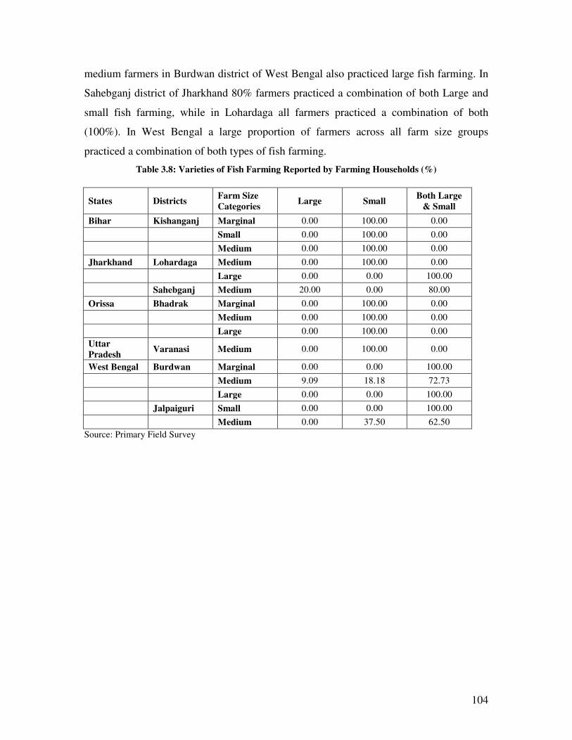
104
medium farmers in Burdwan district of West Bengal also practiced large fish farming. In
Sahebganj district of Jharkhand 80% farmers practiced a combination of both Large and
small fish farming, while in Lohardaga all farmers practiced a combination of both
(100%). In West Bengal a large proportion of farmers across all farm size groups
practiced a combination of both types of fish farming.
Table 3.8: Varieties of Fish Farming Reported by Farming Households (%)
States Districts Farm Size
Categories Large Small
Both Large
& Small
Bihar Kishanganj Marginal 0.00 100.00 0.00
Small 0.00 100.00 0.00
Medium 0.00 100.00 0.00
Jharkhand Lohardaga Medium 0.00 100.00 0.00
Large 0.00 0.00 100.00
Sahebganj Medium 20.00 0.00 80.00
Orissa Bhadrak Marginal 0.00 100.00 0.00
Medium 0.00 100.00 0.00
Large 0.00 100.00 0.00
Uttar
Pradesh Varanasi Medium 0.00 100.00 0.00
West Bengal Burdwan Marginal 0.00 0.00 100.00
Medium 9.09 18.18 72.73
Large 0.00 0.00 100.00
Jalpaiguri Small 0.00 0.00 100.00
Medium 0.00 37.50 62.50
Source: Primary Field Survey
105
Viability of Small Farms
The total household income includes the net income from crop farming, livestock,
fisheries and income from non-farm sources. It may be seen from the Table 3.9 that based
on crop farming alone no farmers earned enough to stay viable.
The shares of monthly income from farm and non-farm sources in the sample
households of the study regions show that income from farm sources is greater than non-
farm sources in all the states of eastern India (Table 3.9). The income from non-farm
sources are the relatively less in the under developed districts compared to the developed
ones in all the selected states.
It is also seen that in all the selected states, except Jharkhand, the net income from
livestock sector is the highest followed by crop farming and then the fisheries. In
Jharkhand, the net income from crop farming was the highest followed by livestock and
fisheries. Further, the net income from livestock is greater than that of crop farming in all
the under developed districts, whereas it is lower than the crop farming in all the
developed districts except the Varanasi district in Uttar Pradesh where income from
livestock was more than the crop farming.
Both income from agriculture and livestock show a positive relationship with
farm size. The income from fisheries was skewed towards medium farmers in the states
of Bihar, Jharkhand and Uttar Pradesh, while in Orissa and West Bengal it showed a
positive relationship with farm size.
It can be seen from the table below that only in the Kishanganj district of Bihar
marginal farmers are earning more income from non-farm sources. In all other states all
categories of farmers are earning more from farm sources. This means that the income of
marginal farmers only in the Kishanganj district of Bihar have shown more vertical
diversification toward non-farm activities whereas overall it is seen that all size classes
show horizontal diversification within agriculture and allied activities.
In the states of Bihar and Uttar Pradesh, only medium farmers have shown more
horizontal diversification toward livestock rearing and fisheries, while in the rest of the
states both medium and large farmers have shown such diversification. Small and
marginal farmers have mainly diversified toward livestock. Only in the states of Bihar
and West Bengal, they have also diversified towards fisheries. Hence, it can be said that
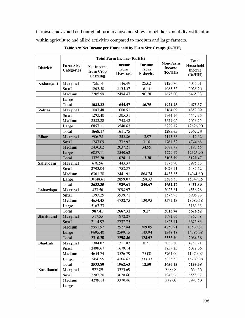
106
in most states small and marginal farmers have not shown much horizontal diversification
within agriculture and allied activities compared to medium and large farmers.
Table 3.9: Net Income per Household by Farm Size Groups (Rs/HH)
Districts Farm Size Categories
Total Farm Income (Rs/HH)
Non-Farm
Income (Rs/HH)
Total
Household Income
(Rs/HH)
Net Income
from Crop Farming
Income
from Livestock
Income
from Fisheries
Kishanganj Marginal 756.14 1146.49 25.62 2126.76 4055.01
Small 1203.50 2135.37 6.13 1683.75 5028.76
Medium 2205.99 2494.47 90.28 1675.00 6465.73
Large
Total 1082.23 1644.47 26.75 1921.93 4675.37
Rohtas Marginal 1087.48 1600.51 2164.09 4852.09
Small 1293.40 1305.31 1844.14 4442.85
Medium 2582.28 1748.42 3329.05 7659.75
Large 6857.11 3540.63 2229.17 12626.90
Total 1668.17 1611.75 2285.65 5565.58
Bihar Marginal 906.75 1352.86 13.97 2143.73 4417.32
Small 1247.09 1732.92 3.16 1761.52 4744.68
Medium 2436.62 2037.21 34.95 2688.77 7197.55
Large 6857.11 3540.63 2229.17 12626.90
Total 1375.20 1628.11 13.38 2103.79 5120.47
Sahebganj Marginal 676.56 1443.37 1875.90 3995.83
Small 2703.04 1758.37 2026.11 6487.52
Medium 6301.30 2441.91 864.74 4433.85 14041.80
Large 10148.61 2859.07 158.33 2583.33 15749.35
Total 3633.35 1929.61 240.67 2652.27 8455.89
Lohardaga Marginal 433.50 2098.97 2023.81 4556.28
Small 1393.25 3939.71 1573.98 6906.93
Medium 4654.45 4732.75 130.95 3571.43 13089.58
Large 5163.33 5163.33
Total 987.41 2667.31 9.17 2012.94 5676.82
Jharkhand Marginal 517.55 1872.27 1972.66 4362.48
Small 2114.97 2737.75 1823.11 6675.83
Medium 5951.97 2927.84 709.09 4250.91 13839.81
Large 9695.40 2599.15 143.94 2348.48 14786.98
Total 2310.38 2298.46 124.92 2332.60 7066.36
Bhadrak Marginal 1384.87 1311.83 0.71 2055.80 4753.21
Small 2499.67 1679.14 1859.25 6038.06
Medium 4654.74 3526.29 25.00 3764.00 11970.02
Large 7456.55 4166.67 333.33 3333.33 15289.88
Total 2533.80 1962.63 12.50 2650.15 7159.08
Kandhamal Marginal 927.89 3373.69 368.08 4669.66
Small 2287.70 3028.60 1242.06 6558.37
Medium 4289.14 3370.46 338.00 7997.60
Large
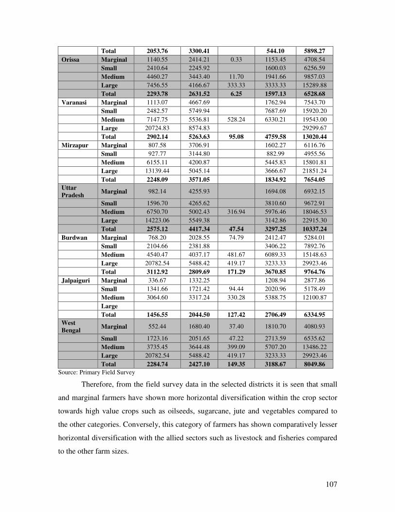
107
Total 2053.76 3300.41 544.10 5898.27
Orissa Marginal 1140.55 2414.21 0.33 1153.45 4708.54
Small 2410.64 2245.92 1600.03 6256.59
Medium 4460.27 3443.40 11.70 1941.66 9857.03
Large 7456.55 4166.67 333.33 3333.33 15289.88
Total 2293.78 2631.52 6.25 1597.13 6528.68
Varanasi Marginal 1113.07 4667.69 1762.94 7543.70
Small 2482.57 5749.94 7687.69 15920.20
Medium 7147.75 5536.81 528.24 6330.21 19543.00
Large 20724.83 8574.83 29299.67
Total 2902.14 5263.63 95.08 4759.58 13020.44
Mirzapur Marginal 807.58 3706.91 1602.27 6116.76
Small 927.77 3144.80 882.99 4955.56
Medium 6155.11 4200.87 5445.83 15801.81
Large 13139.44 5045.14 3666.67 21851.24
Total 2248.09 3571.05 1834.92 7654.05
Uttar
Pradesh Marginal 982.14 4255.93 1694.08 6932.15
Small 1596.70 4265.62 3810.60 9672.91
Medium 6750.70 5002.43 316.94 5976.46 18046.53
Large 14223.06 5549.38 3142.86 22915.30
Total 2575.12 4417.34 47.54 3297.25 10337.24
Burdwan Marginal 768.20 2028.55 74.79 2412.47 5284.01
Small 2104.66 2381.88 3406.22 7892.76
Medium 4540.47 4037.17 481.67 6089.33 15148.63
Large 20782.54 5488.42 419.17 3233.33 29923.46
Total 3112.92 2809.69 171.29 3670.85 9764.76
Jalpaiguri Marginal 336.67 1332.25 1208.94 2877.86
Small 1341.66 1721.42 94.44 2020.96 5178.49
Medium 3064.60 3317.24 330.28 5388.75 12100.87
Large
Total 1456.55 2044.50 127.42 2706.49 6334.95
West
Bengal Marginal 552.44 1680.40 37.40 1810.70 4080.93
Small 1723.16 2051.65 47.22 2713.59 6535.62
Medium 3735.45 3644.48 399.09 5707.20 13486.22
Large 20782.54 5488.42 419.17 3233.33 29923.46
Total 2284.74 2427.10 149.35 3188.67 8049.86
Source: Primary Field Survey
Therefore, from the field survey data in the selected districts it is seen that small
and marginal farmers have shown more horizontal diversification within the crop sector
towards high value crops such as oilseeds, sugarcane, jute and vegetables compared to
the other categories. Conversely, this category of farmers has shown comparatively lesser
horizontal diversification with the allied sectors such as livestock and fisheries compared
to the other farm sizes.
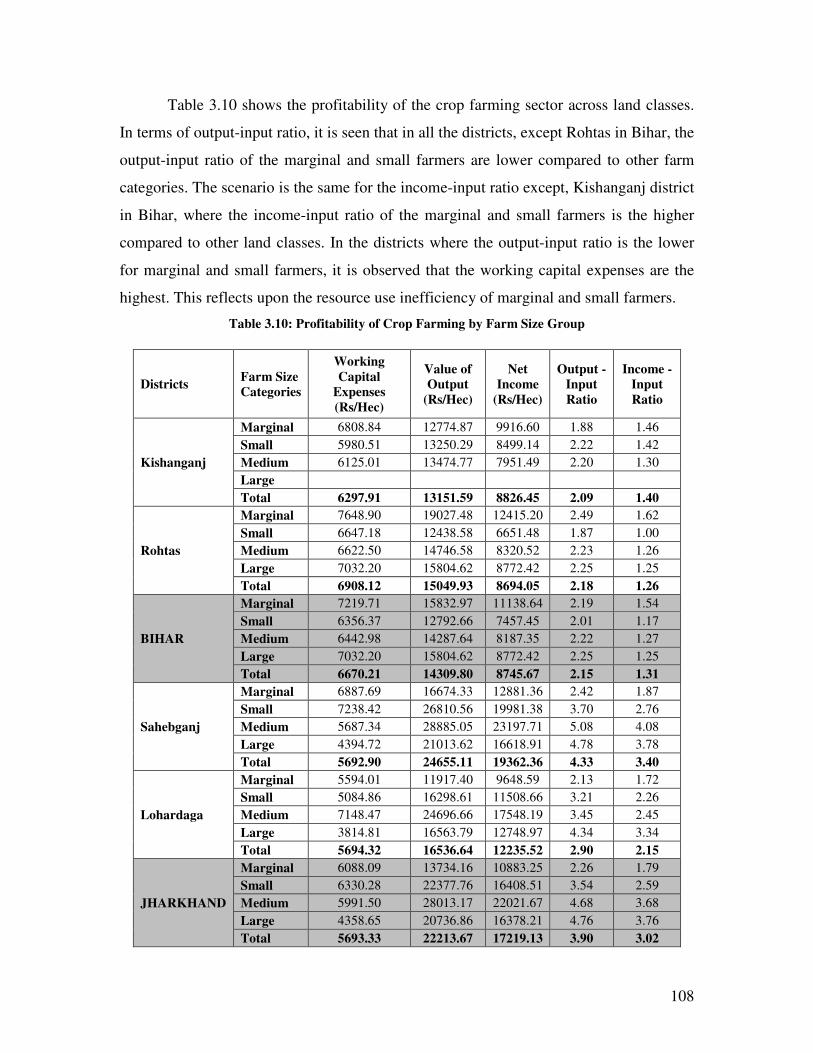
108
Table 3.10 shows the profitability of the crop farming sector across land classes.
In terms of output-input ratio, it is seen that in all the districts, except Rohtas in Bihar, the
output-input ratio of the marginal and small farmers are lower compared to other farm
categories. The scenario is the same for the income-input ratio except, Kishanganj district
in Bihar, where the income-input ratio of the marginal and small farmers is the higher
compared to other land classes. In the districts where the output-input ratio is the lower
for marginal and small farmers, it is observed that the working capital expenses are the
highest. This reflects upon the resource use inefficiency of marginal and small farmers.
Table 3.10: Profitability of Crop Farming by Farm Size Group
Districts Farm Size Categories
Working
Capital Expenses
(Rs/Hec)
Value of Output
(Rs/Hec)
Net Income
(Rs/Hec)
Output - Input
Ratio
Income - Input
Ratio
Kishanganj
Marginal 6808.84 12774.87 9916.60 1.88 1.46
Small 5980.51 13250.29 8499.14 2.22 1.42
Medium 6125.01 13474.77 7951.49 2.20 1.30
Large
Total 6297.91 13151.59 8826.45 2.09 1.40
Rohtas
Marginal 7648.90 19027.48 12415.20 2.49 1.62
Small 6647.18 12438.58 6651.48 1.87 1.00
Medium 6622.50 14746.58 8320.52 2.23 1.26
Large 7032.20 15804.62 8772.42 2.25 1.25
Total 6908.12 15049.93 8694.05 2.18 1.26
BIHAR
Marginal 7219.71 15832.97 11138.64 2.19 1.54
Small 6356.37 12792.66 7457.45 2.01 1.17
Medium 6442.98 14287.64 8187.35 2.22 1.27
Large 7032.20 15804.62 8772.42 2.25 1.25
Total 6670.21 14309.80 8745.67 2.15 1.31
Sahebganj
Marginal 6887.69 16674.33 12881.36 2.42 1.87
Small 7238.42 26810.56 19981.38 3.70 2.76
Medium 5687.34 28885.05 23197.71 5.08 4.08
Large 4394.72 21013.62 16618.91 4.78 3.78
Total 5692.90 24655.11 19362.36 4.33 3.40
Lohardaga
Marginal 5594.01 11917.40 9648.59 2.13 1.72
Small 5084.86 16298.61 11508.66 3.21 2.26
Medium 7148.47 24696.66 17548.19 3.45 2.45
Large 3814.81 16563.79 12748.97 4.34 3.34
Total 5694.32 16536.64 12235.52 2.90 2.15
JHARKHAND
Marginal 6088.09 13734.16 10883.25 2.26 1.79
Small 6330.28 22377.76 16408.51 3.54 2.59
Medium 5991.50 28013.17 22021.67 4.68 3.68
Large 4358.65 20736.86 16378.21 4.76 3.76
Total 5693.33 22213.67 17219.13 3.90 3.02
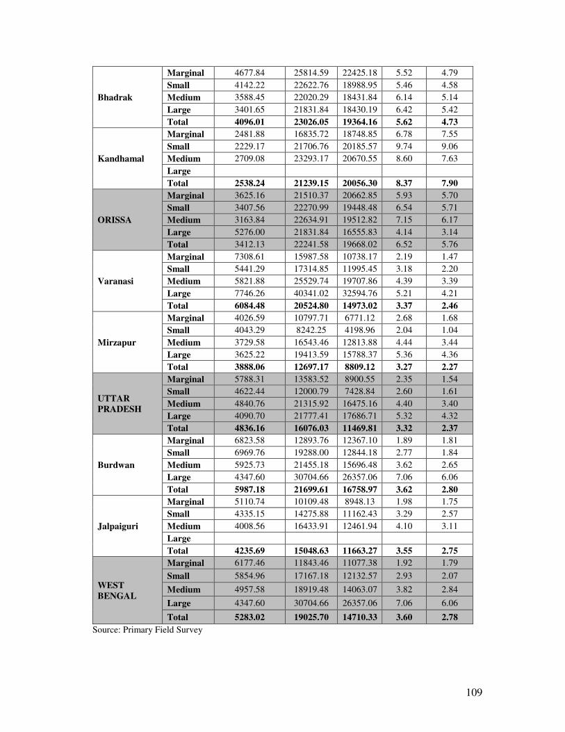
109
Bhadrak
Marginal 4677.84 25814.59 22425.18 5.52 4.79
Small 4142.22 22622.76 18988.95 5.46 4.58
Medium 3588.45 22020.29 18431.84 6.14 5.14
Large 3401.65 21831.84 18430.19 6.42 5.42
Total 4096.01 23026.05 19364.16 5.62 4.73
Kandhamal
Marginal 2481.88 16835.72 18748.85 6.78 7.55
Small 2229.17 21706.76 20185.57 9.74 9.06
Medium 2709.08 23293.17 20670.55 8.60 7.63
Large
Total 2538.24 21239.15 20056.30 8.37 7.90
ORISSA
Marginal 3625.16 21510.37 20662.85 5.93 5.70
Small 3407.56 22270.99 19448.48 6.54 5.71
Medium 3163.84 22634.91 19512.82 7.15 6.17
Large 5276.00 21831.84 16555.83 4.14 3.14
Total 3412.13 22241.58 19668.02 6.52 5.76
Varanasi
Marginal 7308.61 15987.58 10738.17 2.19 1.47
Small 5441.29 17314.85 11995.45 3.18 2.20
Medium 5821.88 25529.74 19707.86 4.39 3.39
Large 7746.26 40341.02 32594.76 5.21 4.21
Total 6084.48 20524.80 14973.02 3.37 2.46
Mirzapur
Marginal 4026.59 10797.71 6771.12 2.68 1.68
Small 4043.29 8242.25 4198.96 2.04 1.04
Medium 3729.58 16543.46 12813.88 4.44 3.44
Large 3625.22 19413.59 15788.37 5.36 4.36
Total 3888.06 12697.17 8809.12 3.27 2.27
UTTAR
PRADESH
Marginal 5788.31 13583.52 8900.55 2.35 1.54
Small 4622.44 12000.79 7428.84 2.60 1.61
Medium 4840.76 21315.92 16475.16 4.40 3.40
Large 4090.70 21777.41 17686.71 5.32 4.32
Total 4836.16 16076.03 11469.81 3.32 2.37
Burdwan
Marginal 6823.58 12893.76 12367.10 1.89 1.81
Small 6969.76 19288.00 12844.18 2.77 1.84
Medium 5925.73 21455.18 15696.48 3.62 2.65
Large 4347.60 30704.66 26357.06 7.06 6.06
Total 5987.18 21699.61 16758.97 3.62 2.80
Jalpaiguri
Marginal 5110.74 10109.48 8948.13 1.98 1.75
Small 4335.15 14275.88 11162.43 3.29 2.57
Medium 4008.56 16433.91 12461.94 4.10 3.11
Large
Total 4235.69 15048.63 11663.27 3.55 2.75
WEST
BENGAL
Marginal 6177.46 11843.46 11077.38 1.92 1.79
Small 5854.96 17167.18 12132.57 2.93 2.07
Medium 4957.58 18919.48 14063.07 3.82 2.84
Large 4347.60 30704.66 26357.06 7.06 6.06
Total 5283.02 19025.70 14710.33 3.60 2.78
Source: Primary Field Survey
110
Small and marginal farmers are diversifying more within the crop sector relative
to other farm categories firstly because, the yields from high value crops mainly
vegetables and sugarcane are higher than food grain crops. Secondly, the returns are more
regular and earlier compared to food grains. Lastly, these farmers, with an abundance of
family labour at their disposal try to maximize their returns from their small holdings by
allocating more acreages to these high value crops whereas large farmers tend to hedge
their bets by devoting more area towards food grains and also diversifying more within
the allied sectors like livestock and fisheries. Despite the benefits of high value crop
diversification for small and marginal farmers, their net incomes from crop farming is
found to be lower than the other farm sizes which indicates inefficient use of resources by
them and also inadequate access to markets for their high value products. Further, the
income even within agriculture and allied activities was skewed in favour of large farms.
It is to be noted that though small and marginal farmers constitute the largest proportion
of farming households in India (including the eastern states), their income from crop
farming and allied sectors (as seen from this field study) was low compared to medium
and large farmers. Further, crop yields also showed a positive relationship with farm size
(including horticultural crops). Small and marginal farmers are diversifying horizontally
within the crop sector, but at the same time more horizontal diversification within the
allied sectors should also be considered to be a viable option for them. Further, their
resource use efficiency within the crop sector has to improve. This can be done by
removing the typical constraints faced by this category of farmers which have been
identified in the next chapter.
111
CHAPTER IV
CONSTRAINTS AND POTENTIALS FOR
AGRICULTURAL DIVERSIFICATION
This chapter attempts to identify the main constraints and potentials underlying
agricultural diversification in the eastern states. At the district level, secondary data
analysis has been done by carrying out several forms of regression exercises. The primary
data analysis for this has been based on farmers’ perception about the constraints faced
by them for agricultural diversification.
Regression Equations
At the district level certain factors were taken to explain agricultural
diversification of value of output from crop production, livestock, forestry and fisheries
through multiple regressions for the triennium ending 2006-07. These factors were
fertilizer consumption, irrigation, annual rainfall, grazing lands, credit, regulated markets,
cold storages, rural roads, rural electrification, veterinary hospitals, forest protection
committees, rural literacy and urban population. This set of regressions taking value of
output could not be worked out for the previouse years because of non-availability of
such data. The regression functions for value of output from various sectors were
estimated as follows;
(i) VCP = f (F, I, R, C, M, R, E, L, U)
Where,
VCP = Value of Output from Crop Production (Rs.)
F = Fertilizer Consumption (Tonnes/Hec)
I = Crop Irrigated Area as a percentage of Gross Cropped Area
R = Average Annual Rainfall (mms)
C = Outstanding Credit (Rs/Hec)
M = Number of Regulated Markets per 1000 Hectares of GCA
R = Length of Rural Roads per 1000 Hectares of GCA
E = Percentage of Electrified Villages
L = Rural Literacy Rate
U= Percentage of Urban Population
112
(ii) VH = f (F, I, R, C, H, R, E, L, U)
Where,
VH = Value of Output from Horticulture (Rs.)
F = Fertilizer Consumption (Tonnes/Hec)
I = Irrigated Area under Horticulture as a percentage of Gross Cropped Area
R = Average Annual Rainfall (mms)
C = Outstanding Credit (Rs/Hec)
H = Number of Village Haats
R = Length of Rural Roads per 1000 Hectares of GCA
E = Percentage of Electrified Villages
L = Rural Literacy Rate
U= Percentage of Urban Population
(iii) VL = f (R, G, C, R, H, E, V, L, U)
Where,
VL = Value of Output from Livestock (Rs.)
R = Average Annual Rainfall (mms)
G = Grazing and Pasture Lands as a percentage of Reported Area
C = Outstanding Credit (Rs/Hec)
R = Length of Rural Roads per 1000 Hectares of GCA
H = Number of Village Haats
E = Percentage of Electrified Villages
V = Number of Veterinary Hospitals
L = Rural Literacy Rate
U= Percentage of Urban Population
(iv) VFO = f (R, C, H, R, E, F, L, U)
Where,
VFO = Value of Output from Forestry (Rs.)
R = Average Annual Rainfall (mms)
C = Outstanding Credit (Rs/Hec)
H = Number of Village Haats
R = Length of Rural Roads per 1000 Hectares of GCA
113
F = Number of Forest Protection Committees
L = Rural Literacy Rate
U= Percentage of Urban Population
(v) VFI = f (R, C, R, S, E, L, U)
Where,
VFI = Value of Output from Fisheries (Rs.)
R = Average Annual Rainfall (mms)
C = Outstanding Credit (Rs/Hec)
R = Length of Rural Roads per 1000 Hectares of GCA
S = Number of Cold Storages
H = Number of Village Haats
E = Percentage of Electrified Villages
L = Rural Literacy Rate
U= Percentage of Urban Population
Furthermore, for better understanding of agricultural diversification in the
previous years at the district level certain factors were taken to explain agricultural
diversification of area under horticultural crops, and livestock per 1000 hectares GCA for
the trienniums ending 1972-73, 1982-83, 1992-93 and 2002-03. The regressions could
not be formulated for the state of Jharkhand due to lack of districtwise data under most
heads.
(i) AFV = f (I, R, C, R, E, L, U)
Where,
AFV = Area under Fruits and Vegetables as a Percentage of GCA
I = Irrigated Area under Fruits & Vegetables as a percentage of Gross Cropped
Area
R = Average Annual Rainfall (mms)
C = Outstanding Credit (Rs/Hec)
R = Length of Rural Roads per 1000 Hectares of GCA
E = Percentage of Electrified Villages
L = Rural Literacy Rate
U= Percentage of Urban Population

114
(ii) L = f(R, C, R, E, L, )
Where,
L = Livestock per 1000 Hec GCA
R = Average Annual Rainfall (mms)
C = Outstanding Credit (Rs/Hec)
R = Length of Rural Roads per 1000 Hectares of GCA
E = Percentage of Electrified Villages
L = Rural Literacy Rate
U= Percentage of Urban Population
Factors Effecting Value of Output of Agriculture & Allied Activities (TE – 2006-07)
Irrigated area as a proportion of GCA showed a positive relationship with the
value of output of total crop production and horticultural crops in the states of Bihar and
Uttar Pradesh. It affected the value of output of only crop production in Orissa and only
horticultural crops in West Bengal. It affected value of output of horticulture and crop
production negatively in Orissa and West Bengal respectively, but the relationship was
not statistically significant at 1% level of significance. In Jharkhand irrigated area
showed a significant negative relationship with both value of output of crop production as
well as horticulture, which indicates that irrigated area is acting as a constraint as a result
of inappropriate water management and inadequate number of irrigations in the state.
Fertilizer use influenced the value of output of total crop production positively
only in the states of Orissa and Uttar Pradesh. In other states its relationship with the
value of output of crop production and horticulture was negative, which indicates the
constraint of imbalanced fertilizer use in these states.
Average annual rainfall affected the value of output of crop production in Uttar
Pradesh and Jharkhand. It showed a positive relationship with the value of output of
horticulture in Bihar, Orissa, Jharkhand and West Bengal. Average annual rainfall also
affects animal husbandry, forestry and fisheries. Hence it showed a positive relationship
with the value of output of livestock in Bihar, Orissa and West Bengal. With respect to
value of output of forestry it showed a positive relationship in Bihar, Uttar Pradesh,
Jharkhand and West Bengal. In Orissa the relationship was negative but not significant at

115
1% level of significance, which shows the importance of rainfall as a major factor
affecting forest resources in eastern India. Rainfall affected the value of output of the
fisheries sector in Bihar, Uttar Pradesh and West Bengal. In the states and sectors where
the relation with rainfall is negative indicates the constraint of insufficient rainfall.
Institutional credit affects the value of output of crop production and horticulture
in all the eastern states, except that in West Bengal the relationship is negative but not
statistically significant at 1% level of significance. This indicates the significance of
institutional credit for crop production & horticulture in eastern India. Institutional credit
also affects animal husbandry, forestry and fisheries. It is an important variable that
positively affects the value of output from livestock. Institutional credit affects the value
of output from forestry in Orissa, Jharkhand and West Bengal. In Bihar and Uttar Pradesh
the relationship is negative but not statistically significant at 1% level. Institutional credit
affects the value of output from fisheries in all the eastern states except Bihar where too
the relationship though negative is not statistically significant at 1% level of significance,
thereby the relevance of institutional credit in the fisheries sector too.
Market density (number of regulated markets per 1000 hec of GCA) could affect
the value of output of only crop production but not the other sectors because the products
from other sectors do not come to regulated markets. It is seen that this factor shows a
positive relationship only in the states of Orissa and Uttar Pradesh. It shows a negative
relationship that is statistically significant at 5% levels in Bihar and Jharkhand and a non-
significant relationship at 1% level West Bengal indicating unavailability of associated
infrastructural facilities like road connectivity and transportation in these states.
Horticultural produce as well as produce from livestock, forestry and fisheries
sector come to village haats rather than regulated markets. Districtwise data on village
haats was found only for the states of Uttar Pradesh and West Bengal. Village haats
showed a positive relationship with the value of output of horticulture, livestock and
fisheries sector in Uttar Pradesh. For the forestry sector in Uttar Pradesh the relationship
was negative though statistically not significant at 1% level of significance. In West
Bengal this relationship was positive for all sectors, thereby indicating the importance of
village haats in agricultural diversification.
116
Percentage of electrified villages showed a positive relationship with the value of
output of crop production in only in the states of Orissa and West Bengal. In Bihar and
Uttar Pradesh the relationship is negative but statistically non-significant at 1% level, but
in Jharkhand it is statistically significant at 5% level of significance. With respect to
horticulture and livestock the relationship is positive only in Orissa, while in the other
states the relationship is negative but statistically not significant at 1% level of
significance. In case of fisheries the relationship is positive in all states except Uttar
Pradesh where too the relationship though negative was statistically not significant at 1%
level of significance. States where percentage of electrified villages showed negative
relationship indicates lack of accessibility of stakeholders to electricity and can also be a
sign of excessive electricity load shedding in these regions.
Rural road density (rural road length per 1000 hec of GCA) shows a positive
relationship with the value of crop production only in Jharkhand and West Bengal. In
Uttar Pradesh and Orissa the relationship is negative but statistically non-significant at
1% level, but in Bihar it is statistically significant at 5% level of significance. Road
density shows a positive relationship with the value of output of horticulture only in Uttar
Pradesh and West Bengal, while in the other states the relationship is negative but not
significant. It shows a positive relationship with the value of output of livestock in Bihar,
and Uttar Pradesh. In West Bengal and Jharkhand the relationship is negative and
statistically non-significant while in Orissa the negative relationship is statistically
significant at 5% level of significance. With respect to the forestry sector, road density
shows a positive relationship only in Orissa, Jharkhand and West Bengal. In Bihar and
Uttar Pradesh the relationship is negative and statistically non-significant at 1% level of
significance. In case of value of output from fisheries, it is seen that the relationship holds
good in Orissa and West Bengal. In Jharkhand the relationship is negative and
statistically significant at 5% level while in Uttar Pradesh and Bihar it is statistically not
significant. States where rural road density showed negative relationship indicates lack
poor road conditions in these states.
Veterinary hospitals and grazing & pasture lands as a percentage of reported area
show a positive relationship with the value of livestock output in all the eastern states
117
except Orissa, where too the relationship though negative is statistically not significant at
1% level of significance.
Percentage of urban population positively affects crop production in Bihar and
Uttar Pradesh. For horticulture it shows a positive relationship in Orissa and Jharkhand.
With respect to livestock the relationship is positively significant only in Orissa. In the
forestry sector it is positive in Orissa, Uttar Pradesh, Jharkhand and West Bengal. In the
fisheries sector it is positive in Bihar, Uttar Pradesh and, Jharkhand.
Rural literacy positively affects crop production only in West Bengal. In the
horticultural sector it is affecting Jharkhand and west Bengal. In the livestock sector it is
positive in Orissa and Jharkhand. In the forestry sector it is positive only in Bihar. In the
fisheries sector it is positive only in Uttar Pradesh. Rural literacy is not affecting
agricultural diversification presumably due to lack of interest in the part of literate youth
in agriculture & allied activities because agriculture is becoming a non-profitable
occupation now (Appendix IV.1).
From this factor analysis, it was seen that in the state of Bihar imbalanced use of
fertilizers was posing a constraint to horticultural diversification. Hence a balanced use of
fertilizers was required, which could be achieved by providing proper training in
horticultural management and practices to farmers. In the state of Jharkhand it was found
inappropriate water management and inadequate water supply was a major constraint
towards horticultural diversification. Thus, in this state proper irrigation facilities are
required. Further, it was found that insufficient rainfall was posing a constraint to
livestock diversification in the state and hence the importance of enhancing irrigation
facilities was needed. Moreover for the fisheries sector poor road conditions, bad road
connectivity and transportation problems in the state have to be improved. In Orissa,
livestock diversification was hindered by road connectivity and transportation problems.
In Orissa, Uttar Pradesh and West Bengal the diversification towards the forestry sector
was mainly constrained by rural literacy rate. This means that as rural literates increase
there is lack of interest in their part to engage themselves in the forestry sector. They
would rather move into the rural non-farm sector (explained in non-farm diversification
in Chapter II (Appendix II.1). In Uttar Pradesh livestock diversification was also
constrained by rural literacy rate.
118
Factors Effecting Area under Horticultural Crops and Livestock Population (TE –
1972)
During the triennium ending 1972 irrigated area under horticulture as a proportion
of GCA showed a positive relationship with the proportion of horticultural area in all the
eastern states. Average annual rainfall showed a positive relationship in Bihar, Orissa and
West Bengal. In the state of Uttar Pradesh the relationship was negative but not
significant at 1% level of significance. Data on institutional credit was not available for
Bihar during this period. Credit showed a positive relationship only in Uttar Pradesh,
while in Orissa it showed a statistically significant result at 1% level, but in West Bengal
the relationship was negative but non-significant. Percentage of villages with electricity
showed a positive relationship only in West Bengal. In the other states it showed a
negative but non-significant relationship. However in Uttar Pradesh the negative
relationship was statistically significant at 1% level of significance. Rural road density
showed a positive relationship in all the states except Orissa where the relationship was
negative and statistically significant at 5% level of significance. Rural literacy rate
showed a positive relationship only in the state of Orissa, while in the other states it
showed a negative though non-significant relationship. Percentage of urban population
showed a positive relationship in Bihar and Orissa, whereas in Uttar Pradesh and West
Bengal it showed a negative relationship, wherein it was statistically significant at 1%
level only in West Bengal.
As regards livestock, during the triennium ending 1972, average annual rainfall
showed a positive relationship with the livestock population per 1000 hec of GCA in
Bihar and Orissa. In the state of Uttar Pradesh and West Bengal the relationship was
negative but not significant at 1% level of significance. Credit showed a positive
relationship in Uttar Pradesh and West Bengal, while in Orissa the relationship was
negative but non-significant. Percentage of villages with electricity showed a negative but
statistically non-significant relationship in all the states. Rural road density showed a
positive relationship in all the states excepting Bihar where the relationship was negative
but statistically non-significant at 1% level of significance. Rural literacy rate showed a
positive relationship in all the states excepting West Bengal where the relationship
though negative was non-significant. Percentage of urban population showed a positive
119
relationship in Bihar and Orissa, whereas in Uttar Pradesh and West Bengal it showed a
negative though non-significant relationship at 1% level of significance (Appendix IV.2).
Factors Effecting Area under Horticultural Crops and Livestock Population (TE –
1982)
During the triennium ending 1982 irrigated area under horticulture as a proportion
of GCA showed a positive relationship with the proportion of horticultural area in all the
eastern states. Average annual rainfall showed a positive relationship in Bihar, Uttar
Pradesh and West Bengal. In the state of Orissa the relationship was negative and
statistically significant at 1% level of significance. Data on institutional credit was not
available for Bihar during this period. Credit showed a positive relationship only in
Orissa, while in Uttar Pradesh and West Bengal it showed a statistically non-significant
result. Percentage of villages with electricity showed a positive relationship only in
Orissa. In the Bihar and West Bengal it showed a negative but non-significant
relationship. However in Uttar Pradesh the negative relationship was statistically
significant at 1% level of significance. Rural road density showed a positive relationship
in all the states. Rural literacy rate showed a positive relationship only in the state of
Orissa, while in the other states it showed a negative though non-significant relationship.
Percentage of urban population showed a negative relationship in all the states, wherein it
was statistically significant at 1% level only in Orissa.
During the triennium ending 1982, average annual rainfall showed a positive
relationship with the livestock population per 1000 hec of GCA only in Uttar Pradesh. In
the state of Bihar the relationship was negative and significant at 1% level of
significance, while in Orissa & West Bengal the negative relationship was not
statistically significant. Credit showed a positive relationship only in West Bengal, while
in Orissa and Uttar Pradesh, the relationship was negative but non-significant. Percentage
of villages with electricity showed a negative but statistically non-significant relationship
only in Bihar and West Bengal, while in Uttar Pradesh the relationship was positive.
Rural road density showed a positive relationship in all the states. Rural literacy rate
showed a positive relationship in Uttar Pradesh and Orissa, while in Bihar and West
Bengal the relationship though negative was non-significant. Percentage of urban
population showed a positive relationship in all states excepting Uttar Pradesh where it
120
showed a negative and statistically significant relationship at 1% level of significance
(Appendix IV.2).
Factors Effecting Area under Horticultural Crops and Livestock Population (TE –
1992)
During the triennium ending 1992 irrigated area under horticulture as a proportion
of GCA showed a positive relationship with the proportion of horticultural area in all the
eastern states. Average annual rainfall showed a positive relationship in Bihar, Uttar
Pradesh and West Bengal. In the state of Orissa the relationship was negative but not
significant at 1% level of significance. Data on institutional credit was not available for
Bihar during this period. Credit showed a positive relationship in Orissa and Uttar
Pradesh, while in West Bengal it showed a negative but statistically non-significant
result. Percentage of villages with electricity showed a positive relationship only in Bihar
and West Bengal. In the Orissa the relationship was negative but non-significant while in
Uttar Pradesh it was statistically significant at 1% level. Rural road density showed a
positive relationship in Bihar and West Bengal while in Orissa and Uttar Pradesh the
relationship was negative and not statistically significant. Rural literacy rate showed a
positive relationship only in the state of Uttar Pradesh, while in the other states it showed
a negative though non-significant relationship. Percentage of urban population showed a
positive relationship in all the states except Bihar where it showed a negative but non-
significant relationship.
As regards livestock, during the triennium 1992, average annual rainfall showed a
positive relationship with the livestock population per 1000 hec of GCA only in the state
of Uttar Pradesh. In the state of Bihar and Orissa the relationship was negative and
significant at 5% level of significance, whereas in West Bengal it was negative but
statistically not significant. Credit showed a positive relationship in Orissa and West
Bengal, while in Uttar Pradesh the relationship was negative and statistically significant
at 5% level of significance. Percentage of villages with electricity showed a negative but
statistically non-significant relationship only in Bihar while it was positive in all the other
states. Rural road density showed a positive relationship in all the states excepting Orissa
where the relationship was negative but statistically non-significant at 1% level of
significance. Rural literacy rate showed a positive relationship in all the states excepting

121
Bihar where the relationship though negative was non-significant. Percentage of urban
population showed a positive relationship only in Orissa, whereas in Uttar Pradesh and
West Bengal it showed a significantly negative relationship at 1% and 5% levels of
significance respectively. In Bihar however, the negative relationship was not statistically
significant (Appendix IV.2).
Factors Effecting Area under Horticultural Crops and Livestock Population (TE –
2002)
During the triennium ending 2002 irrigated area under horticulture as a proportion
of GCA showed a positive relationship with the proportion of horticultural area in all the
eastern states excepting Orissa where the negative relationship was not statistically
significant. Average annual rainfall showed a positive relationship in Bihar and West
Bengal. In the state of Orissa and Uttar Pradesh the relationship was negative but not
significant at 1% level of significance. Institutional credit showed a positive relationship
only in Bihar, while in Orissa it showed a negative and statistically significant result at
1% level, but in Uttar Pradesh and West Bengal the relationship was negative but non-
significant. Percentage of villages with electricity showed a positive relationship in all
states excepting Orissa where too the negative relationship was not statistically
significant at 1% level of significance. Rural road density showed a positive relationship
in Orissa and West Bengal, while in Bihar and Uttar Pradesh the relationship though
negative was not statistically significant at 1% level of significance. Rural literacy rate
showed a positive relationship in the states of Orissa and Uttar Pradesh, while in the other
Bihar and West Bengal it showed a negative relationship statistically significant at 1%
level of significance. Percentage of urban population showed a positive relationship in
West Bengal and Orissa, whereas in Uttar Pradesh and Bihar it showed a negative
relationship, wherein it was statistically significant at 1% level only in Uttar Pradesh.
During the triennium ending 2002, the average annual rainfall showed a positive
relationship with the livestock population per 1000 hec of GCA in all the states.
Institutional credit showed a positive relationship in Bihar and West Bengal, while in
Orissa and Uttar Pradesh the relationship was negative but non-significant. Percentage of
villages with electricity showed a negative but statistically non-significant relationship
only in West Bengal while in all the other states it was positive. Rural road density
122
showed a positive relationship Uttar Pradesh and West Bengal, while in Bihar and Orissa
the relationship was negative but statistically non-significant at 1% level of significance.
Rural literacy rate showed a negative relationship in all the states and was statatistically
significant at 1% level only in Orissa. Percentage of urban population showed a positive
relationship in Bihar and West Bengal, whereas in Uttar Pradesh and Orissa it showed a
negative though non-significant relationship at 1% level of significance (Appendix IV.2).
From this regression analysis of factors constraining area under horticultural crops
and livestock population during the different trienniums, a shift in constraints was
observed over the years. During the triennium ending 1972, in the state of Bihar, lack of
electric supply constrained horticulture and livestock diversification, while timely
availability of credit was the major issue in Orissa. In Uttar Pradesh, horticultural
diversification was constrained by lack of power supply while insufficient rainfall
affected livestock diversification. In West Bengal urban population affected both.
During the triennium ending 1982 and 1992, the constraints affecting horticulture
and livestock diversification differed from the earlier triennium but during these two
trienniums the constraints were nearly the same. In Bihar urban population negatively
affected horticulture while insufficient rainfall affected livestock adversely. In Orissa,
lack of sufficient rainfall affected both. In Uttar Pradesh, lack of power supply affected
the horticulture sector while urban population affected the livestock sector. In West
Bengal, horticulture diversification was mainly affected by unavailability of timely credit
while lack of electricity affected the livestock sector.
During triennium ending 2002, rural literacy rate negatively affected livestock
diversification in all the states. Horticultural diversification was hindered by rural literacy
rate in Bihar and West Bengal, by urban population in Uttar Pradesh and unavailability of
timely credit in Orissa. Therefore this factor analysis shows that in the present times
educated youth are moving out of the traditional sources of income (agriculture and allied
sectors) toward the non-farm sources. Further, timely availability of credit is to be
emphasised for agricultural diversification. It is to be noted that in all the trienniums
irrigation was one of the major factors showing a positive relationship with horticulture
diversification while in the livestock sector road connectivity emerged as the most
123
important factor. Hence the several product and region specific challenges need to be
addressed for enhancing agricultural diversification.
Constraints to Crop Diversification – Based on Field Survey
Tables 4.1 to 4.5 show the percentage of farmers listing major constraints to the
cultivation of fruits, vegetables, flowers and cash crops in the selected districts of Bihar,
Jharkhand, Orissa, Uttar Pradesh and West Bengal.
Constraints to Fruits Cultivation
It can be observed from Table 3.5 that in Bihar (taking both the districts into
account), the major constraints that the majority of farmers faced in the cultivation of
fruits were regarding the non-availability of land, lack of information and knowledge and
lack of timely and proper irrigation. In the Kishanganj district; lack of available land and
lack of information and knowledge were reported to be the major problems. Amongst all
the land classes, the small farmers complained about the availability of land while it was
the marginal farmers who complained about the lack of information and knowledge. In
Rohtas district, the only problem was that of irrigation facilities which hindered the
cultivation of fruits and it was reported by all the categories of farmers. In the state of
Jharkhand, only medium farmers in Lohardaga district complained about the lack of
information and knowledge.
In the state of Orissa, almost all the constraints posed problem in the cultivation
of fruits. In the Bhadrak district, the poor condition of soil was found to be the major
constraint to fruit cultivation followed by the lack of land availability, lack of information
and knowledge and high cost of cultivation. Most of the marginal farmers complained
about the poor soil condition and land not being available and the rest complained about
the lack of information. The small farmers found the high cost of cultivation to be the
major constraint while the medium famers again had the problem with the information
and knowledge. All the large farmers were not happy with the soil condition. In the
Kandhamal district, majority of the farmers reported the lack of information to be the
major constraint followed by labour problems, lack of irrigation, high cost of cultivation
and non-availability of credit. Most of the marginal, small and medium farmers found
lack of information and knowledge to be problematic. Rest of the marginal farmers
complained about labour problems while the rest of the small farmers were worried about
124
the high cost of cultivation and non availability of credit. Amongst the medium farmers,
labour problems were found to be the second most important problem followed by the
lack of irrigation. In both the districts; small and marginal farmers were found to be
facing all the constraints while medium and large farmers complained only about the lack
of information and knowledge and poor condition of soil.
In Uttar Pradesh, all the constraints were found to be posing problem except for
the availability of credit which was not reported even by a single farmer; the labour
problems being the major constraint. Also, the small and marginal farmers in both the
districts were hindered by almost all the constraints. It can also be seen that in both the
districts, non-availability of land posed a problem only for small and medium farmers. In
the Mirzapur district, high cost of cultivation, lack of access to markets, non remunerative
prices and labour problems were reported by all the land classes while only marginal and
small farmers reported soil condition to be a problem. Lack of irrigation was also
reported by all land classes except for large farmers; and most of them who complained
about it were found to be medium farmers. Only small and medium farmers complained
about the land availability. In the Varanasi district, labour problems were found to be the
main problem followed by lack of information and knowledge, high cultivation cost, non-
remunerative prices and lack of land availability. Labour problems were reported by all
the land classes while only marginal farmers complained about land being not available
and only small farmers found non remunerative prices to be a problem. The large farmers
were worried only about labour problems.
In West Bengal, the major constraints to fruit cultivation were the lack of land
availability, lack of information and knowledge and poor soil condition. Also, only
marginal and small farmers were facing the constraints in this state. In the Burdwan
district, all of the small farmers and most of the medium farmers complained about the
non-availability of land while the rest of the medium farmers were concerned about the
poor condition of soil. Whereas in the Jalpaiguri district of West Bengal, the only
constraint was that of poor information sources and was reported by all the marginal and
medium farmers.
125
Table 4.1: Proportion of Farmers Listing Major Constraints to Fruits Cultivation (%)
States Districts Farm Size Categories
Lack of
Land
Availability
Lack of Irrigation
Lack of
Information &
Knowledge
Poor Soil Condition
High Cost
of
Cultivation
Lack of
Market
Accessebility
Non-
Remunerative
Prices
Non-
availibility
of Credit
Labour Problems
Bihar Kishanganj Marginal 0.00 0.00 100.00 0.00 0.00 0.00 0.00 0.00 0.00
Small 100.00 0.00 0.00 0.00 0.00 0.00 0.00 0.00 0.00
Medium 0.00 0.00 0.00 0.00 0.00 0.00 0.00 0.00 0.00
Total 50.00 0.00 50.00 0.00 0.00 0.00 0.00 0.00 0.00
Rohtas Marginal 0.00 100.00 0.00 0.00 0.00 0.00 0.00 0.00 0.00
Small 0.00 100.00 0.00 0.00 0.00 0.00 0.00 0.00 0.00
Medium 0.00 100.00 0.00 0.00 0.00 0.00 0.00 0.00 0.00
Large 0.00 0.00 0.00 0.00 0.00 0.00 0.00 0.00 0.00
Total 0.00 100.00 0.00 0.00 0.00 0.00 0.00 0.00 0.00
Jharkhand Lohardaga Marginal 0.00 0.00 0.00 0.00 0.00 0.00 0.00 0.00 0.00
Small 0.00 0.00 0.00 0.00 0.00 0.00 0.00 0.00 0.00
Medium 0.00 0.00 100.00 0.00 0.00 0.00 0.00 0.00 0.00
Large 0.00 0.00 0.00 0.00 0.00 0.00 0.00 0.00 0.00
Total 0.00 0.00 100.00 0.00 0.00 0.00 0.00 0.00 0.00
Sahebganj Marginal 0.00 0.00 0.00 0.00 0.00 0.00 0.00 0.00 0.00
Small 0.00 0.00 0.00 0.00 0.00 0.00 0.00 0.00 0.00
Medium 0.00 0.00 0.00 0.00 0.00 0.00 0.00 0.00 0.00
Large 0.00 0.00 0.00 0.00 0.00 0.00 0.00 0.00 0.00
Total 0.00 0.00 0.00 0.00 0.00 0.00 0.00 0.00 0.00
Orissa Bhadrak Marginal 40.00 0.00 20.00 40.00 0.00 0.00 0.00 0.00 0.00
Small 0.00 0.00 0.00 0.00 100.00 0.00 0.00 0.00 0.00
Medium 0.00 0.00 100.00 0.00 0.00 0.00 0.00 0.00 0.00
Large 0.00 0.00 0.00 100.00 0.00 0.00 0.00 0.00 0.00
Total 22.22 0.00 22.22 33.33 22.22 0.00 0.00 0.00 0.00
Kandhamal Marginal 0.00 0.00 90.91 0.00 0.00 0.00 0.00 0.00 9.09
126
Small 0.00 0.00 66.67 0.00 16.67 0.00 0.00 16.67 0.00
Medium 0.00 11.11 66.67 0.00 0.00 0.00 0.00 0.00 22.22
Total 0.00 3.85 76.92 0.00 3.85 0.00 0.00 3.85 11.54
Uttar Pradesh
Mirzapur Marginal 12.00 16.00 0.00 4.00 12.00 12.00 8.00 0.00 36.00
Small 7.14 17.86 7.14 0.00 10.71 17.86 14.29 0.00 25.00
Medium 0.00 37.50 0.00 0.00 25.00 12.50 12.50 0.00 12.50
Large 0.00 0.00 0.00 0.00 25.00 25.00 25.00 0.00 25.00
Total 7.69 18.46 3.08 1.54 13.85 15.38 12.31 0.00 27.69
Varanasi Marginal 7.14 0.00 28.57 0.00 14.29 0.00 0.00 0.00 50.00
Small 0.00 0.00 17.65 0.00 11.76 0.00 29.41 0.00 41.18
Medium 0.00 0.00 18.18 0.00 9.09 0.00 0.00 0.00 72.73
Large 0.00 0.00 0.00 0.00 0.00 0.00 0.00 0.00 100.00
Total 2.33 0.00 20.93 0.00 11.63 0.00 11.63 0.00 53.49
West Bengal
Burdwan Small 100.00 0.00 0.00 0.00 0.00 0.00 0.00 0.00 0.00
Medium 60.00 0.00 0.00 40.00 0.00 0.00 0.00 0.00 0.00
Large 0.00 0.00 0.00 0.00 0.00 0.00 0.00 0.00 0.00
Total 66.67 0.00 0.00 33.33 0.00 0.00 0.00 0.00 0.00
Jalpaiguri Marginal 0.00 0.00 100.00 0.00 0.00 0.00 0.00 0.00 0.00
Small 0.00 0.00 0.00 0.00 0.00 0.00 0.00 0.00 0.00
Medium 0.00 0.00 100.00 0.00 0.00 0.00 0.00 0.00 0.00
Total 0.00 0.00 100.00 0.00 0.00 0.00 0.00 0.00 0.00
Source: Primary Field Survey
127
Constraints to Vegetables Cultivation
From Table 4.2 it is seen that in Bihar, the major constraints that hindered the
cultivation of vegetables were lack of timely irrigation, non availability of credit, non-
availability of land and lack of information and knowledge and lack of institutional
support. The small and large farmers faced all these constraints while medium and large
farmers found only lack of available land, lack of institutional support and lack of
irrigation to be problematic. In both the districts, lack of irrigation was found to be the
major constraint, reported by all the categories of farmers. In the Kishanganj district;
majority of the marginal farmers and a small proportion of small farmers found non-
availability of credit to be the second major constraint. Another constraint faced by all the
land classes was the lack of available land. Only marginal farmers found lack of
information and knowledge to be a problem while the constraint related to the lack of
institutional support was reported only by small farmers. In the Rohtas district, apart from
the constraint of lack of irrigation, only a very small proportion of marginal and medium
farmers complained about the non-availability of credit while lack of available land was a
problem only among marginal and small famers. Majority of the large farmers
complained about the lack of institutional support. It can also be noted that in both the
districts; lack of information and knowledge and non-availability of credit was of concern
only amongst small and marginal farmers
In Jharkhand, lack of irrigation was found to be the major constraint hindering the
cultivation of vegetables followed by lack of information and knowledge, high cost of
cultivation and non-availability of land. In the Lohardaga district, all the marginal
farmers and majority of the small farmers found lack of irrigation to be problematic while
the rest of small farmers complained about the non-availability of credit. Amongst the
medium farmers, half of them were worried about the high cost of cultivation and the rest
half had problem with the lack of information and knowledge. In the case of Sahebganj
district, the only problem was that of lack of irrigation and was reported by all the
categories of farmers except for the large farmers. It can also be noticed that in both the
districts, large farmers did not complain about any of the constraint. Further, the farm
level data of this state again reveals the same fact that the small and marginal farmers
were constrained by almost all the factors effecting cultivation of vegetables in this state.
128
In the state of Orissa, the major constraints effecting the vegetable cultivation
were found to be high cultivation cost, lack of available land, lack of information and
knowledge and poor soil condition. Also, all these constraints affected the marginal and
small farmers while only one or two of them affected the medium farmers and none
affected the large farmers. In Bhadrak district, high cost of cultivation was found to be
the major constraint affecting the vegetable cultivation reported by most of the small
farmers and all the medium farmers. Majority of the marginal farmers complained about
the lack of available land and the poor condition of soil. The rest of the marginal farmers
and one third of the small farmers were not happy with the irrigation condition. In the
Khandamal district, lack of irrigation and lack of information and knowledge were
reported to be the major constraints by all the categories of farmers. Lack of available
land was also reported by all the farm classes (except large farmers) and only few
marginal farmers were not happy with the soil condition.
In Uttar Pradesh, small and marginal farmers were hit by all the constraints that
affected the cultivation of vegetables in this state. In the Mirzapur district, all the
categories of farmers reported lack of irrigation to be the major constraint affecting the
vegetable cultivation. High cultivation cost was found to be the second major constraint
(reported by all the land classes) followed by lack of market accessibility and lack of
information and knowledge (again reported by all except large farmers). Only marginal
farmers found lack of land availability to be a problem while only small farmers reported
the crops destroyed by insects or animals to be a concern. In the Varanasi district, all the
land classes reported lack of institutional support to be the major constraint while non-
remunerative prices was found to be the second major constraint (reported by all the
categories of farmers) followed by lack of information and knowledge which was
reported only by marginal farmers. Thus in Uttar Pradesh, lack of available land, crops
destroyed by insects/ animals and lack of information and knowledge were reported only
by small and marginal farmers.
In the state of West Bengal, the small and marginal farmers found non-availability
of land, lack of institutional support, lack of irrigation, lack of access to local markets to
be the major constraints. In the Burdwan district, non-availability of land was found to be
the major constraint reported by all the categories of farmers. All the land classes except
129
the large farmers found lack of irrigation to be the second major constraint followed by
non-availability of credit and lack of market accessibility, both of which were reported
only by marginal farmers. Lack of institutional support was found to be the problem only
among the marginal farmers. In the Jalpaiguri district, all the marginal and most of the
small and medium farmers reported lack of irrigation to be the major constraint followed
by non-remunerative prices which was reported only by one-third of the medium farmers.
The rest of the small farmers found lack of institutional support to be problematic.
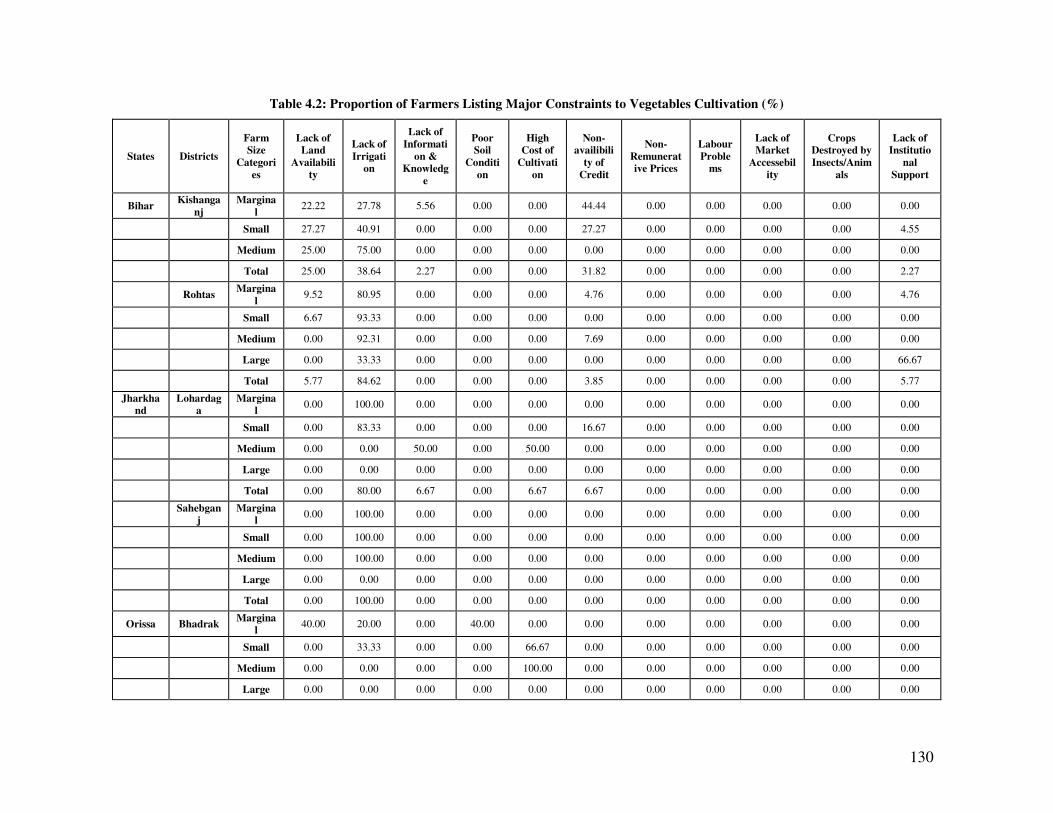
130
Table 4.2: Proportion of Farmers Listing Major Constraints to Vegetables Cultivation (%)
States Districts
Farm Size
Categori
es
Lack of Land
Availabili
ty
Lack of
Irrigation
Lack of
Informati
on & Knowledg
e
Poor Soil
Conditi
on
High Cost of
Cultivati
on
Non-availibili
ty of
Credit
Non-
Remunerative Prices
Labour
Problems
Lack of Market
Accessebil
ity
Crops Destroyed by
Insects/Anim
als
Lack of Institutio
nal
Support
Bihar Kishanga
nj
Margina
l 22.22 27.78 5.56 0.00 0.00 44.44 0.00 0.00 0.00 0.00 0.00
Small 27.27 40.91 0.00 0.00 0.00 27.27 0.00 0.00 0.00 0.00 4.55
Medium 25.00 75.00 0.00 0.00 0.00 0.00 0.00 0.00 0.00 0.00 0.00
Total 25.00 38.64 2.27 0.00 0.00 31.82 0.00 0.00 0.00 0.00 2.27
Rohtas Margina
l 9.52 80.95 0.00 0.00 0.00 4.76 0.00 0.00 0.00 0.00 4.76
Small 6.67 93.33 0.00 0.00 0.00 0.00 0.00 0.00 0.00 0.00 0.00
Medium 0.00 92.31 0.00 0.00 0.00 7.69 0.00 0.00 0.00 0.00 0.00
Large 0.00 33.33 0.00 0.00 0.00 0.00 0.00 0.00 0.00 0.00 66.67
Total 5.77 84.62 0.00 0.00 0.00 3.85 0.00 0.00 0.00 0.00 5.77
Jharkhand
Lohardaga
Marginal
0.00 100.00 0.00 0.00 0.00 0.00 0.00 0.00 0.00 0.00 0.00
Small 0.00 83.33 0.00 0.00 0.00 16.67 0.00 0.00 0.00 0.00 0.00
Medium 0.00 0.00 50.00 0.00 50.00 0.00 0.00 0.00 0.00 0.00 0.00
Large 0.00 0.00 0.00 0.00 0.00 0.00 0.00 0.00 0.00 0.00 0.00
Total 0.00 80.00 6.67 0.00 6.67 6.67 0.00 0.00 0.00 0.00 0.00
Sahebgan
j Margina
l 0.00 100.00 0.00 0.00 0.00 0.00 0.00 0.00 0.00 0.00 0.00
Small 0.00 100.00 0.00 0.00 0.00 0.00 0.00 0.00 0.00 0.00 0.00
Medium 0.00 100.00 0.00 0.00 0.00 0.00 0.00 0.00 0.00 0.00 0.00
Large 0.00 0.00 0.00 0.00 0.00 0.00 0.00 0.00 0.00 0.00 0.00
Total 0.00 100.00 0.00 0.00 0.00 0.00 0.00 0.00 0.00 0.00 0.00
Orissa Bhadrak Margina
l 40.00 20.00 0.00 40.00 0.00 0.00 0.00 0.00 0.00 0.00 0.00
Small 0.00 33.33 0.00 0.00 66.67 0.00 0.00 0.00 0.00 0.00 0.00
Medium 0.00 0.00 0.00 0.00 100.00 0.00 0.00 0.00 0.00 0.00 0.00
Large 0.00 0.00 0.00 0.00 0.00 0.00 0.00 0.00 0.00 0.00 0.00
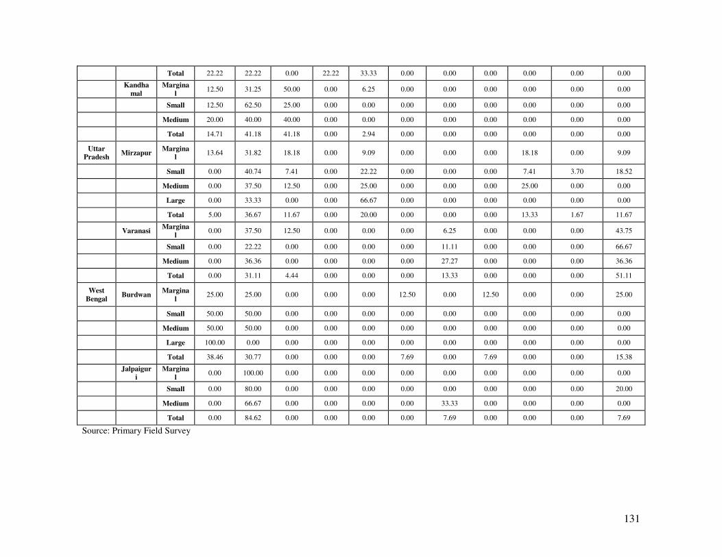
131
Total 22.22 22.22 0.00 22.22 33.33 0.00 0.00 0.00 0.00 0.00 0.00
Kandha
mal
Margina
l 12.50 31.25 50.00 0.00 6.25 0.00 0.00 0.00 0.00 0.00 0.00
Small 12.50 62.50 25.00 0.00 0.00 0.00 0.00 0.00 0.00 0.00 0.00
Medium 20.00 40.00 40.00 0.00 0.00 0.00 0.00 0.00 0.00 0.00 0.00
Total 14.71 41.18 41.18 0.00 2.94 0.00 0.00 0.00 0.00 0.00 0.00
Uttar Pradesh
Mirzapur Margina
l 13.64 31.82 18.18 0.00 9.09 0.00 0.00 0.00 18.18 0.00 9.09
Small 0.00 40.74 7.41 0.00 22.22 0.00 0.00 0.00 7.41 3.70 18.52
Medium 0.00 37.50 12.50 0.00 25.00 0.00 0.00 0.00 25.00 0.00 0.00
Large 0.00 33.33 0.00 0.00 66.67 0.00 0.00 0.00 0.00 0.00 0.00
Total 5.00 36.67 11.67 0.00 20.00 0.00 0.00 0.00 13.33 1.67 11.67
Varanasi Margina
l 0.00 37.50 12.50 0.00 0.00 0.00 6.25 0.00 0.00 0.00 43.75
Small 0.00 22.22 0.00 0.00 0.00 0.00 11.11 0.00 0.00 0.00 66.67
Medium 0.00 36.36 0.00 0.00 0.00 0.00 27.27 0.00 0.00 0.00 36.36
Total 0.00 31.11 4.44 0.00 0.00 0.00 13.33 0.00 0.00 0.00 51.11
West
Bengal Burdwan
Margina
l 25.00 25.00 0.00 0.00 0.00 12.50 0.00 12.50 0.00 0.00 25.00
Small 50.00 50.00 0.00 0.00 0.00 0.00 0.00 0.00 0.00 0.00 0.00
Medium 50.00 50.00 0.00 0.00 0.00 0.00 0.00 0.00 0.00 0.00 0.00
Large 100.00 0.00 0.00 0.00 0.00 0.00 0.00 0.00 0.00 0.00 0.00
Total 38.46 30.77 0.00 0.00 0.00 7.69 0.00 7.69 0.00 0.00 15.38
Jalpaigur
i
Margina
l 0.00 100.00 0.00 0.00 0.00 0.00 0.00 0.00 0.00 0.00 0.00
Small 0.00 80.00 0.00 0.00 0.00 0.00 0.00 0.00 0.00 0.00 20.00
Medium 0.00 66.67 0.00 0.00 0.00 0.00 33.33 0.00 0.00 0.00 0.00
Total 0.00 84.62 0.00 0.00 0.00 0.00 7.69 0.00 0.00 0.00 7.69
Source: Primary Field Survey
132
Constraints to Flowers Cultivation
From Table 4.3 it is seen that in Bihar, lack of irrigation and lack of information
and knowledge were observed to be the major constraints hindering flower cultivation.
The small and marginal farmers were found tot be suffering from both the constraints. In
the Kishanganj district, only marginal farmers reported and they complained about the
lack of information and knowledge. In the Rohtas district, all the small and medium
farmers found lack of irrigation to be the major concern.
In Jharkhand, poor soil condition was found to be the most important constraint
followed by lack of information and knowledge and high cultivation cost. In the
Lohardaga district, only medium farmers reported and all of them were not happy with
the condition of soil. In the Sahebganj district, all the small farmers found lack of
information and knowledge to be problematic while all the medium farmers complained
about the lack of access to local markets.
In Orissa; lack of irrigation was found to be the major constraint affecting flower
cultivation in both the districts. Further, all the constraints were reported by marginal and
small farmers while large farmers did not face even a single constraint. In the Bhadrak
district, majority of the marginal farmers complained about the non-availability of land
and poor soil condition while the rest of them reported lack of information and
knowledge to be a concern. All the small farmers found the high cost of cultivation to be
a problem while all the medium farmers complained about the lack of information and
knowledge. In the Khandamal district, lack of information and knowledge to be the major
constraint (reported by all the marginal, small and most of the medium farmers) followed
by lack of access to local markets (reported by the rest of the medium farmers).
In the state of Uttar Pradesh,; all the constraints posed problem for the small and
marginal farmers except for the poor soil condition which was not reported even by a
single farmer. In the Mirzapur district, high cultivation cost and labour problems were
found to be the major constraints reported by all the categories of farmers. Most of the
marginal farmers and small farmers complained about the lack of information and
knowledge. Only marginal farmers had problem with non-availability of land and non-
availability of credit. Lack of market accessibility and lack of institutional support were
reported only by marginal and small farmers. All the land classes except for large farmers

133
complained about the lack of irrigation. Another constraint that troubled all the land
classes was that of the non-remunerative prices. In the Varanasi district, lack of
information and knowledge was found to be the major constraint reported by all the land
classes. A very small proportion of medium farmers complained about the labour
problems. Lack of institutional support was found to be the problem by all except large
farmers. Only marginal farmers complained about the lack of irrigation and non-
remunerative prices, while high cultivation cost and lack of access to markets were
reported only by small farmers. Taking both the districts into account, the small and
marginal farmers were slightly better off in Varanasi, where they complained only about
four constraints compared to the Mirzapur district. Even though the small and marginal
farmers were slightly better off in Varanasi, they still lagged behind medium and large
farmers in both the districts.
In West Bengal; in the Burdwan district, lack of information and knowledge, lack
of market accessibility and lack of available land were found to be the major constraints
affecting flower cultivation. Most of the marginal farmers complained about the lack of
information and knowledge while the rest one-third of them reported lack of access to
markets to be a problem. Majority of the medium farmers reported lack of available land
and lack of market accessibility to be problematic while the rest of them complained
about the lack of information and knowledge. In the Jalpaiguri district, lack of access to
markets was observed to be the major constraint followed by lack of information and
knowledge and lack of irrigation. Most of the marginal farmers and around one-fifth of
the medium farmers reported lack of information and knowledge to be a problem. Rest of
the marginal farmers complained about the lack of irrigation. Lack of access to local
markets was reported by most of the medium farmers.

134
Table 4.3: Proportion of Farmers Listing Major Constraints to Flowers Cultivation (%)
States Districts
Farm Size
Categories
Lack of Land
Availability
Lack of Irrigati
on
Lack of Informati
on &
Knowledge
Poor Soil
Condition
High Cost of
Cultivation
Lack of Market
Accessibility
Non-availibili
ty of Credit
Lack of Institutio
nal Support
Labour Proble
ms
Non-remunerati
ve Prices
Bihar Kishanga
nj
Margina
l 0.00 0.00 100.00 0.00 0.00 0.00 0.00 0.00 0.00 0.00
Small 0.00 0.00 0.00 0.00 0.00 0.00 0.00 0.00 0.00 0.00
Medium 0.00 0.00 0.00 0.00 0.00 0.00 0.00 0.00 0.00 0.00
Total 0.00 0.00 100.00 0.00 0.00 0.00 0.00 0.00 0.00 0.00
Rohtas Margina
l 0.00 0.00 0.00 0.00 0.00 0.00 0.00 0.00 0.00 0.00
Small 0.00 100.00 0.00 0.00 0.00 0.00 0.00 0.00 0.00 0.00
Medium 0.00 100.00 0.00 0.00 0.00 0.00 0.00 0.00 0.00 0.00
Large 0.00 0.00 0.00 0.00 0.00 0.00 0.00 0.00 0.00 0.00
Total 0.00 100.00 0.00 0.00 0.00 0.00 0.00 0.00 0.00 0.00
Jharkhand
Lohardaga
Marginal
0.00 0.00 0.00 0.00 0.00 0.00 0.00 0.00 0.00 0.00
Small 0.00 0.00 0.00 0.00 0.00 0.00 0.00 0.00 0.00 0.00
Medium 0.00 0.00 0.00 100.00 0.00 0.00 0.00 0.00 0.00 0.00
Large 0.00 0.00 0.00 0.00 0.00 0.00 0.00 0.00 0.00 0.00
Total 0.00 0.00 0.00 100.00 0.00 0.00 0.00 0.00 0.00 0.00
Sahebganj
Marginal
0.00 0.00 0.00 0.00 0.00 0.00 0.00 0.00 0.00 0.00
Small 0.00 0.00 100.00 0.00 0.00 0.00 0.00 0.00 0.00 0.00
Medium 0.00 0.00 0.00 0.00 0.00 100.00 0.00 0.00 0.00 0.00
Large 0.00 0.00 0.00 0.00 0.00 0.00 0.00 0.00 0.00 0.00
Total 0.00 0.00 50.00 0.00 0.00 50.00 0.00 0.00 0.00 0.00
Orissa Bhadrak Marginal
40.00 0.00 20.00 40.00 0.00 0.00 0.00 0.00 0.00 0.00
Small 0.00 0.00 0.00 0.00 100.00 0.00 0.00 0.00 0.00 0.00
Medium 0.00 0.00 100.00 0.00 0.00 0.00 0.00 0.00 0.00 0.00
Large 0.00 0.00 0.00 0.00 0.00 0.00 0.00 0.00 0.00 0.00
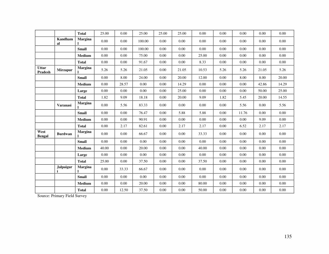
135
Total 25.00 0.00 25.00 25.00 25.00 0.00 0.00 0.00 0.00 0.00
Kandham
al
Margina
l 0.00 0.00 100.00 0.00 0.00 0.00 0.00 0.00 0.00 0.00
Small 0.00 0.00 100.00 0.00 0.00 0.00 0.00 0.00 0.00 0.00
Medium 0.00 0.00 75.00 0.00 0.00 25.00 0.00 0.00 0.00 0.00
Total 0.00 0.00 91.67 0.00 0.00 8.33 0.00 0.00 0.00 0.00
Uttar
Pradesh Mirzapur
Margina
l 5.26 5.26 21.05 0.00 21.05 10.53 5.26 5.26 21.05 5.26
Small 0.00 8.00 24.00 0.00 20.00 12.00 0.00 8.00 8.00 20.00
Medium 0.00 28.57 0.00 0.00 14.29 0.00 0.00 0.00 42.86 14.29
Large 0.00 0.00 0.00 0.00 25.00 0.00 0.00 0.00 50.00 25.00
Total 1.82 9.09 18.18 0.00 20.00 9.09 1.82 5.45 20.00 14.55
Varanasi Margina
l 0.00 5.56 83.33 0.00 0.00 0.00 0.00 5.56 0.00 5.56
Small 0.00 0.00 76.47 0.00 5.88 5.88 0.00 11.76 0.00 0.00
Medium 0.00 0.00 90.91 0.00 0.00 0.00 0.00 0.00 9.09 0.00
Total 0.00 2.17 82.61 0.00 2.17 2.17 0.00 6.52 2.17 2.17
West
Bengal Burdwan
Margina
l 0.00 0.00 66.67 0.00 0.00 33.33 0.00 0.00 0.00 0.00
Small 0.00 0.00 0.00 0.00 0.00 0.00 0.00 0.00 0.00 0.00
Medium 40.00 0.00 20.00 0.00 0.00 40.00 0.00 0.00 0.00 0.00
Large 0.00 0.00 0.00 0.00 0.00 0.00 0.00 0.00 0.00 0.00
Total 25.00 0.00 37.50 0.00 0.00 37.50 0.00 0.00 0.00 0.00
Jalpaigur
i
Margina
l 0.00 33.33 66.67 0.00 0.00 0.00 0.00 0.00 0.00 0.00
Small 0.00 0.00 0.00 0.00 0.00 0.00 0.00 0.00 0.00 0.00
Medium 0.00 0.00 20.00 0.00 0.00 80.00 0.00 0.00 0.00 0.00
Total 0.00 12.50 37.50 0.00 0.00 50.00 0.00 0.00 0.00 0.00
Source: Primary Field Survey
136
Constraints to Cash Crops Cultivation
From Table 4.4 it is seen that in the state of Bihar, the only constraint to cash crop
cultivation was found to be lack of irrigation and it was reported by all the small farmers
from the Rohtas district.
In Jharkhand, labour problems, lack of information and knowledge and non
remunerative prices were reported to be the major constraints affecting the cash crop
cultivation. In the Lohardaga district, all the marginal farmers complained about the non
remunerative prices while all the medium farmers found the lack of information and
knowledge to be problematic. In the Sahebganj district, all the large farmers complained
about the labour related problems.
In the state of Orissa, in the Bhadrak district, lack of irrigation was found to be the
major constraint reported by half of the marginal and small farmers. Rest half of the small
farmers and approximately one-third of the medium farmers found high cultivation cost
to be problematic. Lack of available land and poor soil condition were reported by rest of
the marginal farmers. Only medium farmers complained about the lack of information
and knowledge and non-remunerative prices. All the large farmers reported about the
labour related problems. In the Khandamal district, lack of information and knowledge
were found to be the major constraint. It was reported by most of the marginal, half of the
medium and all the small farmers. Rest of the marginal farmers complained about the
lack of land availability. For the medium farmers, lack of irrigation was the second major
constraint followed by non-availability of land and non-remunerative prices.
In the state of Uttar Pradesh, the small and marginal farmers were constrained by
all the factors except for non-remunerative prices. In the Mirzapur district, lack of market
accessibility was of major concern followed by lack of information and knowledge and
lack of institutional support reported by all the land classes. High cost of cultivation was
found to be affecting all the land classes except the large farmers. Only medium farmers
had problem with the labour and the poor condition of soil while only marginal farmers
complained about the land not being available. Non-availability of credit was found to be
the second major constraint for marginal and small farmers. In the Varanasi district, lack
of institutional support was found to be the most important constraint affecting majority
of the marginal farmers and one-fifth of the small farmers. Most of the small farmers also
137
found lack of information and knowledge and non-availability of credit to be problematic
while all the medium farmers complained about the lack of access to markets. It can
further be noted that in both the districts, only small and marginal farmers did not have
enough land and enough credit to cultivate cash crops.
In the state of West Bengal, in the Burdwan district, lack of available land was
reported to be the major problem affecting cash crop cultivation. It was reported by
majority of the small farmers and all the medium farmers. Half of the marginal farmers
complained about the non-availability of credit while the rest half were worried about the
non remunerative prices. Lack of irrigation and lack of access to markets were reported
only by small farmers. In the Jalpaiguri district, non-availability of credit and the
institutional related problems were the major constraints reported by the marginal and the
medium farmers. All the small farmers complained about the non-remunerative prices
while lack of irrigation was reported only by one-third of the medium farmers.
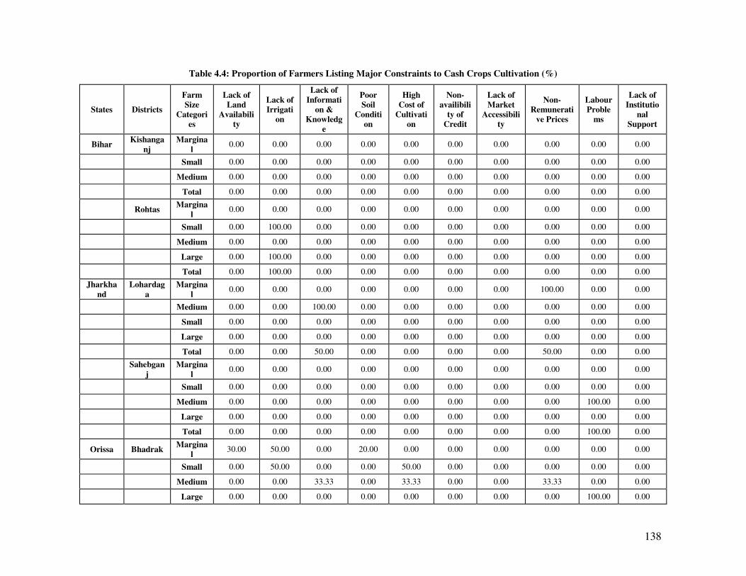
138
Table 4.4: Proportion of Farmers Listing Major Constraints to Cash Crops Cultivation (%)
States Districts
Farm Size
Categories
Lack of Land
Availability
Lack of Irrigati
on
Lack of
Information &
Knowledge
Poor Soil
Condition
High Cost of
Cultivation
Non-availibili
ty of Credit
Lack of Market
Accessibility
Non-Remunerati
ve Prices
Labour Proble
ms
Lack of Institutio
nal Support
Bihar Kishanga
nj
Margina
l 0.00 0.00 0.00 0.00 0.00 0.00 0.00 0.00 0.00 0.00
Small 0.00 0.00 0.00 0.00 0.00 0.00 0.00 0.00 0.00 0.00
Medium 0.00 0.00 0.00 0.00 0.00 0.00 0.00 0.00 0.00 0.00
Total 0.00 0.00 0.00 0.00 0.00 0.00 0.00 0.00 0.00 0.00
Rohtas Margina
l 0.00 0.00 0.00 0.00 0.00 0.00 0.00 0.00 0.00 0.00
Small 0.00 100.00 0.00 0.00 0.00 0.00 0.00 0.00 0.00 0.00
Medium 0.00 0.00 0.00 0.00 0.00 0.00 0.00 0.00 0.00 0.00
Large 0.00 100.00 0.00 0.00 0.00 0.00 0.00 0.00 0.00 0.00
Total 0.00 100.00 0.00 0.00 0.00 0.00 0.00 0.00 0.00 0.00
Jharkha
nd
Lohardag
a
Margina
l 0.00 0.00 0.00 0.00 0.00 0.00 0.00 100.00 0.00 0.00
Medium 0.00 0.00 100.00 0.00 0.00 0.00 0.00 0.00 0.00 0.00
Small 0.00 0.00 0.00 0.00 0.00 0.00 0.00 0.00 0.00 0.00
Large 0.00 0.00 0.00 0.00 0.00 0.00 0.00 0.00 0.00 0.00
Total 0.00 0.00 50.00 0.00 0.00 0.00 0.00 50.00 0.00 0.00
Sahebgan
j
Margina
l 0.00 0.00 0.00 0.00 0.00 0.00 0.00 0.00 0.00 0.00
Small 0.00 0.00 0.00 0.00 0.00 0.00 0.00 0.00 0.00 0.00
Medium 0.00 0.00 0.00 0.00 0.00 0.00 0.00 0.00 100.00 0.00
Large 0.00 0.00 0.00 0.00 0.00 0.00 0.00 0.00 0.00 0.00
Total 0.00 0.00 0.00 0.00 0.00 0.00 0.00 0.00 100.00 0.00
Orissa Bhadrak Margina
l 30.00 50.00 0.00 20.00 0.00 0.00 0.00 0.00 0.00 0.00
Small 0.00 50.00 0.00 0.00 50.00 0.00 0.00 0.00 0.00 0.00
Medium 0.00 0.00 33.33 0.00 33.33 0.00 0.00 33.33 0.00 0.00
Large 0.00 0.00 0.00 0.00 0.00 0.00 0.00 0.00 100.00 0.00

139
Total 16.67 38.89 5.56 11.11 16.67 0.00 0.00 5.56 5.56 0.00
Kandham
al
Margina
l 16.67 0.00 83.33 0.00 0.00 0.00 0.00 0.00 0.00 0.00
Small 0.00 0.00 100.00 0.00 0.00 0.00 0.00 0.00 0.00 0.00
Medium 10.00 30.00 50.00 0.00 0.00 0.00 0.00 10.00 0.00 0.00
Total 11.11 11.11 74.07 0.00 0.00 0.00 0.00 3.70 0.00 0.00
Uttar
Pradesh Mirzapur
Margina
l 5.88 5.88 17.65 0.00 11.76 17.65 23.53 0.00 11.76 5.88
Small 0.00 12.50 16.67 0.00 8.33 16.67 25.00 0.00 0.00 20.83
Medium 0.00 12.50 25.00 12.50 12.50 0.00 12.50 0.00 12.50 12.50
Large 0.00 25.00 25.00 0.00 0.00 0.00 25.00 0.00 0.00 25.00
Total 1.89 11.32 18.87 1.89 9.43 13.21 22.64 0.00 5.66 15.09
Varanasi Margina
l 16.67 0.00 0.00 16.67 0.00 33.33 0.00 0.00 0.00 33.33
Small 0.00 0.00 40.00 0.00 0.00 40.00 0.00 0.00 0.00 20.00
Medium 0.00 0.00 0.00 0.00 0.00 0.00 100.00 0.00 0.00 0.00
Total 8.33 0.00 16.67 8.33 0.00 33.33 8.33 0.00 0.00 25.00
West
Bengal Burdwan
Margina
l 0.00 0.00 0.00 0.00 0.00 50.00 0.00 50.00 0.00 0.00
Small 33.33 33.33 0.00 0.00 0.00 0.00 33.33 0.00 0.00 0.00
Medium 100.00 0.00 0.00 0.00 0.00 0.00 0.00 0.00 0.00 0.00
Large 0.00 0.00 0.00 0.00 0.00 0.00 0.00 0.00 0.00 0.00
Total 42.86 14.29 0.00 0.00 0.00 14.29 14.29 14.29 0.00 0.00
Jalpaigur
i
Margina
l 0.00 0.00 0.00 0.00 0.00 50.00 0.00 0.00 0.00 50.00
Small 0.00 0.00 0.00 0.00 0.00 0.00 0.00 100.00 0.00 0.00
Medium 0.00 33.33 0.00 0.00 0.00 33.33 0.00 0.00 0.00 33.33
Total 0.00 16.67 0.00 0.00 0.00 33.33 0.00 16.67 0.00 33.33
Source: Primary Field Survey
140
Constraints to Livestock Diversification
Table 4.5 lists out the major constraints towards diversification of livestock in the
study regions. It is observed that non-availability of credit in time is reported to be the
major constraint towards diversification of livestock by majority of the small and
marginal farming households in the Kishangarh district of Bihar and Bhadrak district of
Orissa. Lack of proper veterinary services is the major constraint towards Livestock
diversification by small and marginal farmers in the Kandhamal district of Orissa, and in
both districts of Uttar Pradesh. Lack of proper feed is the major constraint for small and
marginal farmers in both districts of Jharkhand, Uttar Pradesh and Jalpaiguri district of
West Bengal. Non-remunerative prices are the major constraint for small and marginal
farmers in the Rohtas district of Bihar and Burdwan district of West Bengal. The
constraint of non-availability of credit on time and non-availability of proper feed is
found to be usually inversely related to farm size in the study regions. Medium and large
farmers also reported non-remunerative prices to be a constraint.
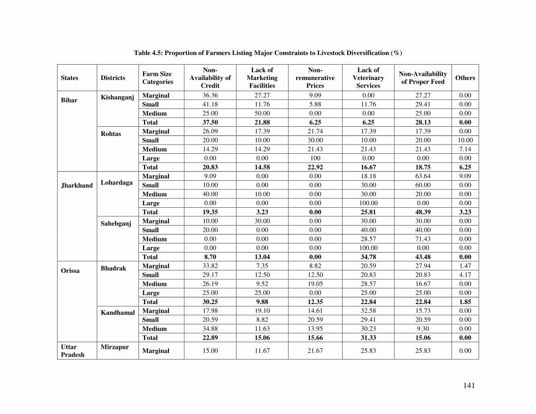
141
Table 4.5: Proportion of Farmers Listing Major Constraints to Livestock Diversification (%)
States Districts Farm Size
Categories
Non-
Availability of
Credit
Lack of
Marketing
Facilities
Non-
remunerative
Prices
Lack of
Veterinary
Services
Non-Availability
of Proper Feed Others
Bihar
Kishanganj
Marginal 36.36 27.27 9.09 0.00 27.27 0.00
Small 41.18 11.76 5.88 11.76 29.41 0.00
Medium 25.00 50.00 0.00 0.00 25.00 0.00
Total 37.50 21.88 6.25 6.25 28.13 0.00
Rohtas
Marginal 26.09 17.39 21.74 17.39 17.39 0.00
Small 20.00 10.00 30.00 10.00 20.00 10.00
Medium 14.29 14.29 21.43 21.43 21.43 7.14
Large 0.00 0.00 100 0.00 0.00 0.00
Total 20.83 14.58 22.92 16.67 18.75 6.25
Jharkhand
Lohardaga
Marginal 9.09 0.00 0.00 18.18 63.64 9.09
Small 10.00 0.00 0.00 30.00 60.00 0.00
Medium 40.00 10.00 0.00 30.00 20.00 0.00
Large 0.00 0.00 0.00 100.00 0.00 0.00
Total 19.35 3.23 0.00 25.81 48.39 3.23
Sahebganj
Marginal 10.00 30.00 0.00 30.00 30.00 0.00
Small 20.00 0.00 0.00 40.00 40.00 0.00
Medium 0.00 0.00 0.00 28.57 71.43 0.00
Large 0.00 0.00 0.00 100.00 0.00 0.00
Total 8.70 13.04 0.00 34.78 43.48 0.00
Orissa
Bhadrak
Marginal 33.82 7.35 8.82 20.59 27.94 1.47
Small 29.17 12.50 12.50 20.83 20.83 4.17
Medium 26.19 9.52 19.05 28.57 16.67 0.00
Large 25.00 25.00 0.00 25.00 25.00 0.00
Total 30.25 9.88 12.35 22.84 22.84 1.85
Kandhamal
Marginal 17.98 19.10 14.61 32.58 15.73 0.00
Small 20.59 8.82 20.59 29.41 20.59 0.00
Medium 34.88 11.63 13.95 30.23 9.30 0.00
Total 22.89 15.06 15.66 31.33 15.06 0.00
Uttar
Pradesh
Mirzapur
Marginal 15.00 11.67 21.67 25.83 25.83 0.00
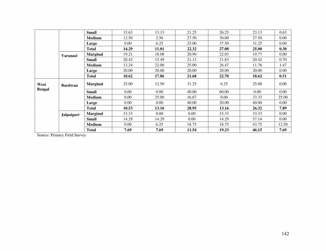
142
Small 15.63 13.13 21.25 26.25 23.13 0.63
Medium 12.50 2.50 27.50 30.00 27.50 0.00
Large 0.00 6.25 25.00 37.50 31.25 0.00
Total 14.29 11.01 22.32 27.08 25.00 0.30
Varanasi
Marginal 19.21 18.08 20.90 22.03 19.77 0.00
Small 20.42 15.49 21.13 21.83 20.42 0.70
Medium 13.24 22.06 25.00 26.47 11.76 1.47
Large 20.00 20.00 20.00 20.00 20.00 0.00
Total 18.62 17.86 21.68 22.70 18.62 0.51
West Bengal
Burdwan
Marginal 25.00 12.50 31.25 6.25 25.00 0.00
Small 0.00 0.00 40.00 60.00 0.00 0.00
Medium 0.00 25.00 16.67 0.00 33.33 25.00
Large 0.00 0.00 40.00 20.00 40.00 0.00
Total 10.53 13.16 28.95 13.16 26.32 7.89
Jalpaiguri
Marginal 33.33 0.00 0.00 33.33 33.33 0.00
Small 14.29 14.29 0.00 14.29 57.14 0.00
Medium 0.00 6.25 18.75 18.75 43.75 12.50
Total 7.69 7.69 11.54 19.23 46.15 7.69
Source: Primary Field Survey
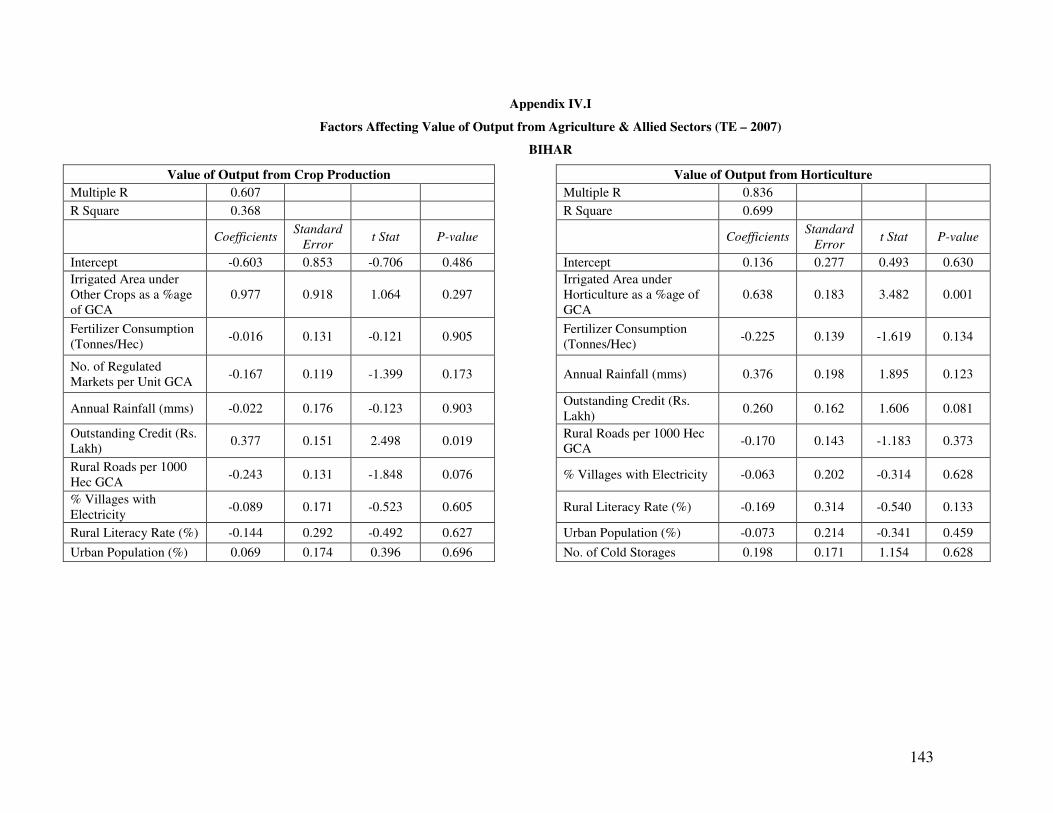
143
Appendix IV.I
Factors Affecting Value of Output from Agriculture & Allied Sectors (TE – 2007)
BIHAR
Value of Output from Crop Production Value of Output from Horticulture
Multiple R 0.607 Multiple R 0.836
R Square 0.368 R Square 0.699
Coefficients Standard
Error t Stat P-value Coefficients
Standard
Error t Stat P-value
Intercept -0.603 0.853 -0.706 0.486 Intercept 0.136 0.277 0.493 0.630
Irrigated Area under
Other Crops as a %age
of GCA
0.977 0.918 1.064 0.297
Irrigated Area under
Horticulture as a %age of
GCA
0.638 0.183 3.482 0.001
Fertilizer Consumption
(Tonnes/Hec) -0.016 0.131 -0.121 0.905
Fertilizer Consumption
(Tonnes/Hec) -0.225 0.139 -1.619 0.134
No. of Regulated
Markets per Unit GCA -0.167 0.119 -1.399 0.173 Annual Rainfall (mms) 0.376 0.198 1.895 0.123
Annual Rainfall (mms) -0.022 0.176 -0.123 0.903 Outstanding Credit (Rs.
Lakh) 0.260 0.162 1.606 0.081
Outstanding Credit (Rs.
Lakh) 0.377 0.151 2.498 0.019
Rural Roads per 1000 Hec
GCA -0.170 0.143 -1.183 0.373
Rural Roads per 1000
Hec GCA -0.243 0.131 -1.848 0.076 % Villages with Electricity -0.063 0.202 -0.314 0.628
% Villages with
Electricity -0.089 0.171 -0.523 0.605 Rural Literacy Rate (%) -0.169 0.314 -0.540 0.133
Rural Literacy Rate (%) -0.144 0.292 -0.492 0.627 Urban Population (%) -0.073 0.214 -0.341 0.459
Urban Population (%) 0.069 0.174 0.396 0.696 No. of Cold Storages 0.198 0.171 1.154 0.628
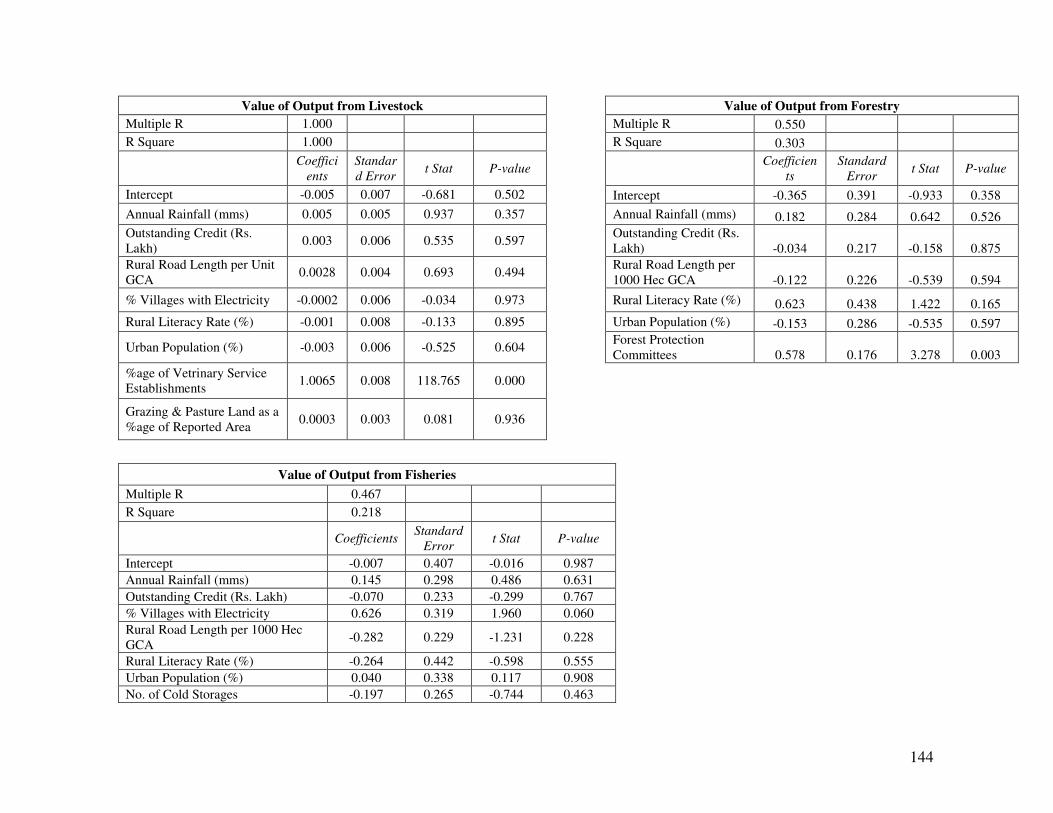
144
Value of Output from Livestock Value of Output from Forestry
Multiple R 1.000 Multiple R 0.550
R Square 1.000 R Square 0.303
Coeffici
ents
Standar
d Error t Stat P-value
Coefficien
ts
Standard
Error t Stat P-value
Intercept -0.005 0.007 -0.681 0.502 Intercept -0.365 0.391 -0.933 0.358
Annual Rainfall (mms) 0.005 0.005 0.937 0.357 Annual Rainfall (mms) 0.182 0.284 0.642 0.526
Outstanding Credit (Rs.
Lakh) 0.003 0.006 0.535 0.597
Outstanding Credit (Rs.
Lakh) -0.034 0.217 -0.158 0.875
Rural Road Length per Unit
GCA 0.0028 0.004 0.693 0.494
Rural Road Length per
1000 Hec GCA -0.122 0.226 -0.539 0.594
% Villages with Electricity -0.0002 0.006 -0.034 0.973 Rural Literacy Rate (%) 0.623 0.438 1.422 0.165
Rural Literacy Rate (%) -0.001 0.008 -0.133 0.895 Urban Population (%) -0.153 0.286 -0.535 0.597
Urban Population (%) -0.003 0.006 -0.525 0.604 Forest Protection
Committees 0.578 0.176 3.278 0.003
%age of Vetrinary Service
Establishments 1.0065 0.008 118.765 0.000
Grazing & Pasture Land as a
%age of Reported Area 0.0003 0.003 0.081 0.936
Value of Output from Fisheries
Multiple R 0.467
R Square 0.218
Coefficients Standard
Error t Stat P-value
Intercept -0.007 0.407 -0.016 0.987
Annual Rainfall (mms) 0.145 0.298 0.486 0.631
Outstanding Credit (Rs. Lakh) -0.070 0.233 -0.299 0.767
% Villages with Electricity 0.626 0.319 1.960 0.060
Rural Road Length per 1000 Hec
GCA -0.282 0.229 -1.231 0.228
Rural Literacy Rate (%) -0.264 0.442 -0.598 0.555
Urban Population (%) 0.040 0.338 0.117 0.908
No. of Cold Storages -0.197 0.265 -0.744 0.463
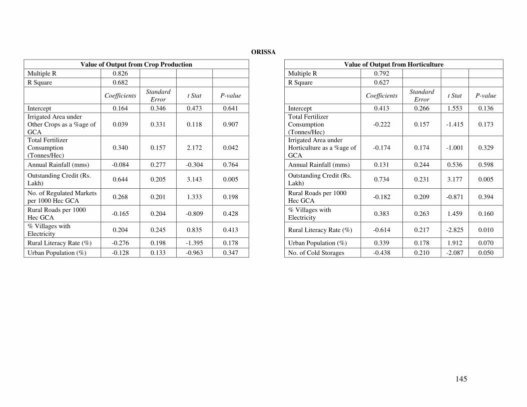
145
ORISSA
Value of Output from Crop Production Value of Output from Horticulture
Multiple R 0.826 Multiple R 0.792
R Square 0.682 R Square 0.627
Coefficients Standard
Error t Stat P-value Coefficients
Standard
Error t Stat P-value
Intercept 0.164 0.346 0.473 0.641 Intercept 0.413 0.266 1.553 0.136
Irrigated Area under
Other Crops as a %age of
GCA
0.039 0.331 0.118 0.907
Total Fertilizer
Consumption
(Tonnes/Hec)
-0.222 0.157 -1.415 0.173
Total Fertilizer
Consumption
(Tonnes/Hec)
0.340 0.157 2.172 0.042
Irrigated Area under
Horticulture as a %age of
GCA
-0.174 0.174 -1.001 0.329
Annual Rainfall (mms) -0.084 0.277 -0.304 0.764 Annual Rainfall (mms) 0.131 0.244 0.536 0.598
Outstanding Credit (Rs.
Lakh) 0.644 0.205 3.143 0.005
Outstanding Credit (Rs.
Lakh) 0.734 0.231 3.177 0.005
No. of Regulated Markets
per 1000 Hec GCA 0.268 0.201 1.333 0.198
Rural Roads per 1000
Hec GCA -0.182 0.209 -0.871 0.394
Rural Roads per 1000
Hec GCA -0.165 0.204 -0.809 0.428
% Villages with
Electricity 0.383 0.263 1.459 0.160
% Villages with
Electricity 0.204 0.245 0.835 0.413 Rural Literacy Rate (%) -0.614 0.217 -2.825 0.010
Rural Literacy Rate (%) -0.276 0.198 -1.395 0.178 Urban Population (%) 0.339 0.178 1.912 0.070
Urban Population (%) -0.128 0.133 -0.963 0.347 No. of Cold Storages -0.438 0.210 -2.087 0.050
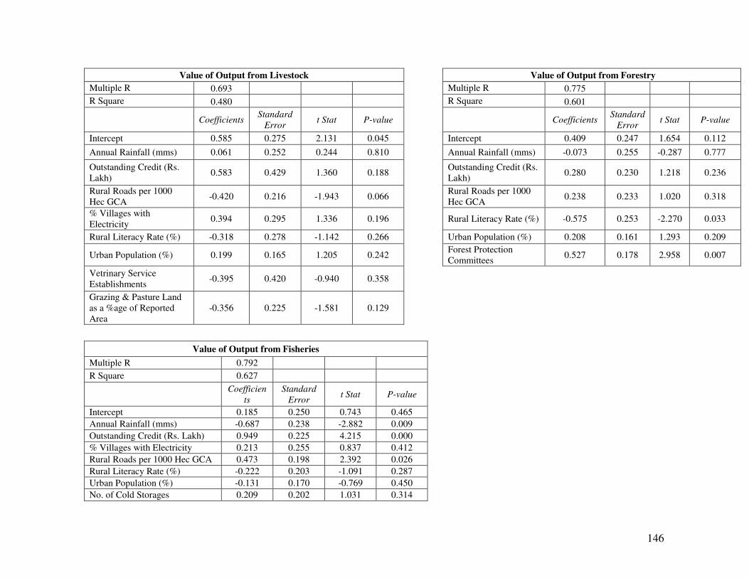
146
Value of Output from Livestock Value of Output from Forestry
Multiple R 0.693 Multiple R 0.775
R Square 0.480 R Square 0.601
Coefficients Standard
Error t Stat P-value Coefficients
Standard
Error t Stat P-value
Intercept 0.585 0.275 2.131 0.045 Intercept 0.409 0.247 1.654 0.112
Annual Rainfall (mms) 0.061 0.252 0.244 0.810 Annual Rainfall (mms) -0.073 0.255 -0.287 0.777
Outstanding Credit (Rs.
Lakh) 0.583 0.429 1.360 0.188
Outstanding Credit (Rs.
Lakh) 0.280 0.230 1.218 0.236
Rural Roads per 1000
Hec GCA -0.420 0.216 -1.943 0.066
Rural Roads per 1000
Hec GCA 0.238 0.233 1.020 0.318
% Villages with
Electricity 0.394 0.295 1.336 0.196 Rural Literacy Rate (%) -0.575 0.253 -2.270 0.033
Rural Literacy Rate (%) -0.318 0.278 -1.142 0.266 Urban Population (%) 0.208 0.161 1.293 0.209
Urban Population (%) 0.199 0.165 1.205 0.242 Forest Protection
Committees 0.527 0.178 2.958 0.007
Vetrinary Service
Establishments -0.395 0.420 -0.940 0.358
Grazing & Pasture Land
as a %age of Reported
Area
-0.356 0.225 -1.581 0.129
Value of Output from Fisheries
Multiple R 0.792
R Square 0.627
Coefficien
ts
Standard
Error t Stat P-value
Intercept 0.185 0.250 0.743 0.465
Annual Rainfall (mms) -0.687 0.238 -2.882 0.009
Outstanding Credit (Rs. Lakh) 0.949 0.225 4.215 0.000
% Villages with Electricity 0.213 0.255 0.837 0.412
Rural Roads per 1000 Hec GCA 0.473 0.198 2.392 0.026
Rural Literacy Rate (%) -0.222 0.203 -1.091 0.287
Urban Population (%) -0.131 0.170 -0.769 0.450
No. of Cold Storages 0.209 0.202 1.031 0.314
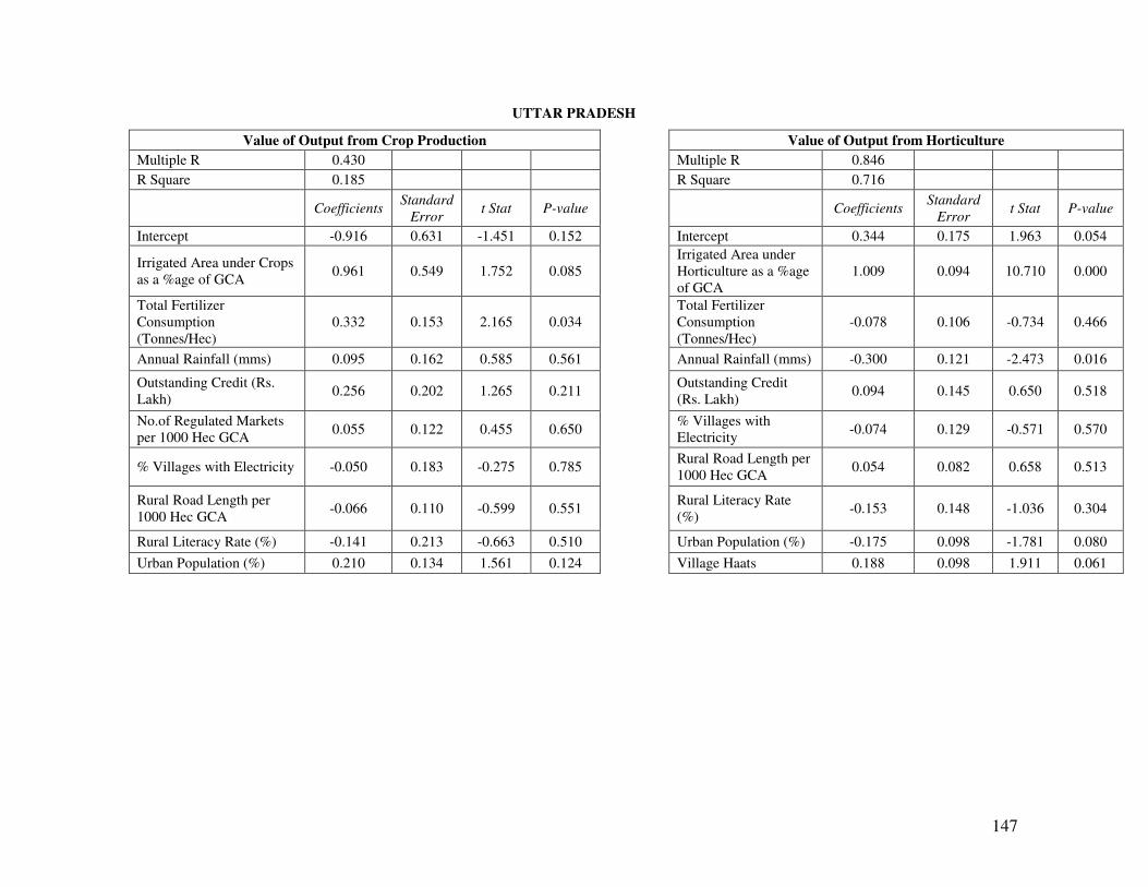
147
UTTAR PRADESH
Value of Output from Crop Production Value of Output from Horticulture
Multiple R 0.430 Multiple R 0.846
R Square 0.185 R Square 0.716
Coefficients Standard
Error t Stat P-value Coefficients
Standard
Error t Stat P-value
Intercept -0.916 0.631 -1.451 0.152 Intercept 0.344 0.175 1.963 0.054
Irrigated Area under Crops
as a %age of GCA 0.961 0.549 1.752 0.085
Irrigated Area under
Horticulture as a %age
of GCA
1.009 0.094 10.710 0.000
Total Fertilizer
Consumption
(Tonnes/Hec)
0.332 0.153 2.165 0.034
Total Fertilizer
Consumption
(Tonnes/Hec)
-0.078 0.106 -0.734 0.466
Annual Rainfall (mms) 0.095 0.162 0.585 0.561 Annual Rainfall (mms) -0.300 0.121 -2.473 0.016
Outstanding Credit (Rs.
Lakh) 0.256 0.202 1.265 0.211
Outstanding Credit
(Rs. Lakh) 0.094 0.145 0.650 0.518
No.of Regulated Markets
per 1000 Hec GCA 0.055 0.122 0.455 0.650
% Villages with
Electricity -0.074 0.129 -0.571 0.570
% Villages with Electricity -0.050 0.183 -0.275 0.785 Rural Road Length per
1000 Hec GCA 0.054 0.082 0.658 0.513
Rural Road Length per
1000 Hec GCA -0.066 0.110 -0.599 0.551
Rural Literacy Rate
(%) -0.153 0.148 -1.036 0.304
Rural Literacy Rate (%) -0.141 0.213 -0.663 0.510 Urban Population (%) -0.175 0.098 -1.781 0.080
Urban Population (%) 0.210 0.134 1.561 0.124 Village Haats 0.188 0.098 1.911 0.061
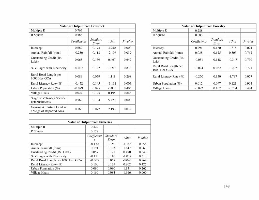
148
Value of Output from Livestock Value of Output from Forestry
Multiple R 0.767 Multiple R 0.288
R Square 0.588 R Square 0.083
Coefficients Standard
Error t Stat P-value Coefficients
Standard
Error t Stat P-value
Intercept 0.682 0.173 3.950 0.000 Intercept 0.291 0.160 1.818 0.074
Annual Rainfall (mms) -0.250 0.118 -2.106 0.039 Annual Rainfall (mms) 0.038 0.125 0.305 0.762
Outstanding Credit (Rs.
Lakh) 0.065 0.139 0.467 0.642
Outstanding Credit (Rs.
Lakh) -0.051 0.148 -0.347 0.730
% Villages with Electricity -0.027 0.127 -0.212 0.833 Rural Road Length per
1000 Hec GCA -0.024 0.082 -0.292 0.771
Rural Road Length per
1000 Hec GCA 0.089 0.079 1.118 0.268 Rural Literacy Rate (%) -0.270 0.150 -1.797 0.077
Rural Literacy Rate (%) -0.452 0.145 -3.111 0.003 Urban Population (%) 0.012 0.097 0.121 0.904
Urban Population (%) -0.079 0.095 -0.836 0.406 Village Haats -0.072 0.102 -0.704 0.484
Village Haats 0.024 0.125 0.195 0.846
%age of Vetrinary Service
Establishments 0.562 0.104 5.423 0.000
Grazing & Pasture Land as
a %age of Reported Area 0.168 0.077 2.193 0.032
Value of Output from Fisheries
Multiple R 0.422
R Square 0.178
Coefficient
s
Standard
Error t Stat P-value
Intercept -0.172 0.150 -1.146 0.256
Annual Rainfall (mms) 0.191 0.103 1.847 0.069
Outstanding Credit (Rs. Lakh) 0.057 0.121 0.470 0.640
% Villages with Electricity -0.111 0.110 -1.017 0.313
Rural Road Length per 1000 Hec GCA -0.003 0.068 -0.045 0.964
Rural Literacy Rate (%) 0.100 0.125 0.802 0.425
Urban Population (%) 0.090 0.080 1.131 0.262
Village Haats 0.160 0.084 1.916 0.060
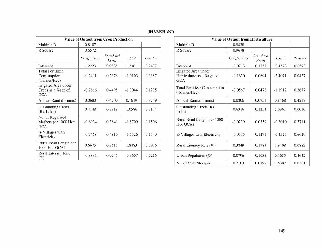
149
JHARKHAND
Value of Output from Crop Production Value of Output from Horticulture
Multiple R 0.8107 Multiple R 0.9838
R Square 0.6572 R Square 0.9678
Coefficients Standard
Error t Stat P-value Coefficients
Standard
Error t Stat P-value
Intercept 1.2223 0.9888 1.2361 0.2477 Intercept -0.0713 0.1557 -0.4578 0.6593
Total Fertilizer
Consumption
(Tonnes/Hec)
-0.2401 0.2376 -1.0103 0.3387
Irrigated Area under
Horticulture as a %age of
GCA
-0.1670 0.0694 -2.4071 0.0427
Irrigated Area under
Crops as a %age of
GCA
-0.7666 0.4498 -1.7044 0.1225 Total Fertilizer Consumption
(Tonnes/Hec) -0.0567 0.0476 -1.1912 0.2677
Annual Rainfall (mms) 0.0680 0.4200 0.1619 0.8749 Annual Rainfall (mms) 0.0806 0.0951 0.8468 0.4217
Outstanding Credit
(Rs. Lakh) 0.4148 0.3919 1.0586 0.3174
Outstanding Credit (Rs.
Lakh) 0.6316 0.1254 5.0361 0.0010
No. of Regulated
Markets per 1000 Hec
GCA
-0.6034 0.3841 -1.5709 0.1506 Rural Road Length per 1000
Hec GCA) -0.0229 0.0759 -0.3010 0.7711
% Villages with
Electricity -0.7468 0.4810 -1.5526 0.1549 % Villages with Electricity -0.0575 0.1271 -0.4525 0.6629
Rural Road Length per
1000 Hec GCA) 0.6675 0.3611 1.8483 0.0976 Rural Literacy Rate (%) 0.3849 0.1983 1.9408 0.0882
Rural Literacy Rate
(%) -0.3335 0.9245 -0.3607 0.7266 Urban Population (%) 0.0796 0.1035 0.7685 0.4642
No. of Cold Storages 0.2103 0.0799 2.6307 0.0301
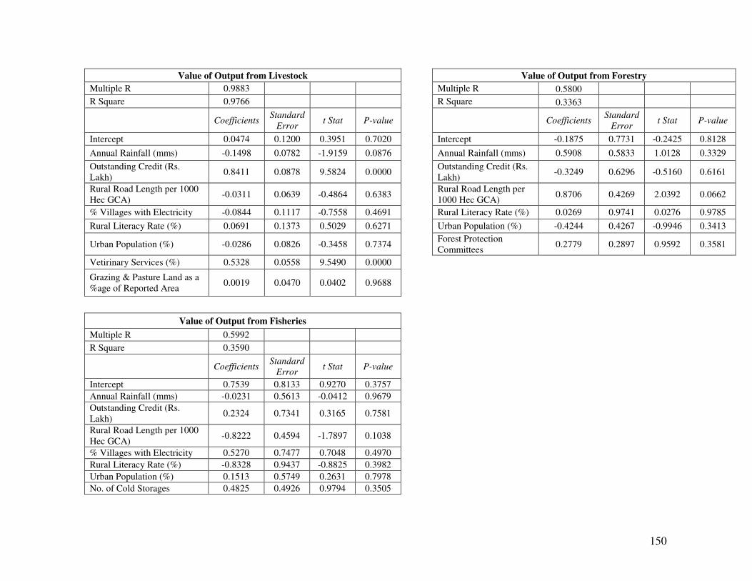
150
Value of Output from Livestock Value of Output from Forestry
Multiple R 0.9883 Multiple R 0.5800
R Square 0.9766 R Square 0.3363
Coefficients Standard
Error t Stat P-value Coefficients
Standard
Error t Stat P-value
Intercept 0.0474 0.1200 0.3951 0.7020 Intercept -0.1875 0.7731 -0.2425 0.8128
Annual Rainfall (mms) -0.1498 0.0782 -1.9159 0.0876 Annual Rainfall (mms) 0.5908 0.5833 1.0128 0.3329
Outstanding Credit (Rs.
Lakh) 0.8411 0.0878 9.5824 0.0000
Outstanding Credit (Rs.
Lakh) -0.3249 0.6296 -0.5160 0.6161
Rural Road Length per 1000
Hec GCA) -0.0311 0.0639 -0.4864 0.6383
Rural Road Length per
1000 Hec GCA) 0.8706 0.4269 2.0392 0.0662
% Villages with Electricity -0.0844 0.1117 -0.7558 0.4691 Rural Literacy Rate (%) 0.0269 0.9741 0.0276 0.9785
Rural Literacy Rate (%) 0.0691 0.1373 0.5029 0.6271 Urban Population (%) -0.4244 0.4267 -0.9946 0.3413
Urban Population (%) -0.0286 0.0826 -0.3458 0.7374 Forest Protection
Committees 0.2779 0.2897 0.9592 0.3581
Vetirinary Services (%) 0.5328 0.0558 9.5490 0.0000
Grazing & Pasture Land as a
%age of Reported Area 0.0019 0.0470 0.0402 0.9688
Value of Output from Fisheries
Multiple R 0.5992
R Square 0.3590
Coefficients Standard
Error t Stat P-value
Intercept 0.7539 0.8133 0.9270 0.3757
Annual Rainfall (mms) -0.0231 0.5613 -0.0412 0.9679
Outstanding Credit (Rs.
Lakh) 0.2324 0.7341 0.3165 0.7581
Rural Road Length per 1000
Hec GCA) -0.8222 0.4594 -1.7897 0.1038
% Villages with Electricity 0.5270 0.7477 0.7048 0.4970
Rural Literacy Rate (%) -0.8328 0.9437 -0.8825 0.3982
Urban Population (%) 0.1513 0.5749 0.2631 0.7978
No. of Cold Storages 0.4825 0.4926 0.9794 0.3505
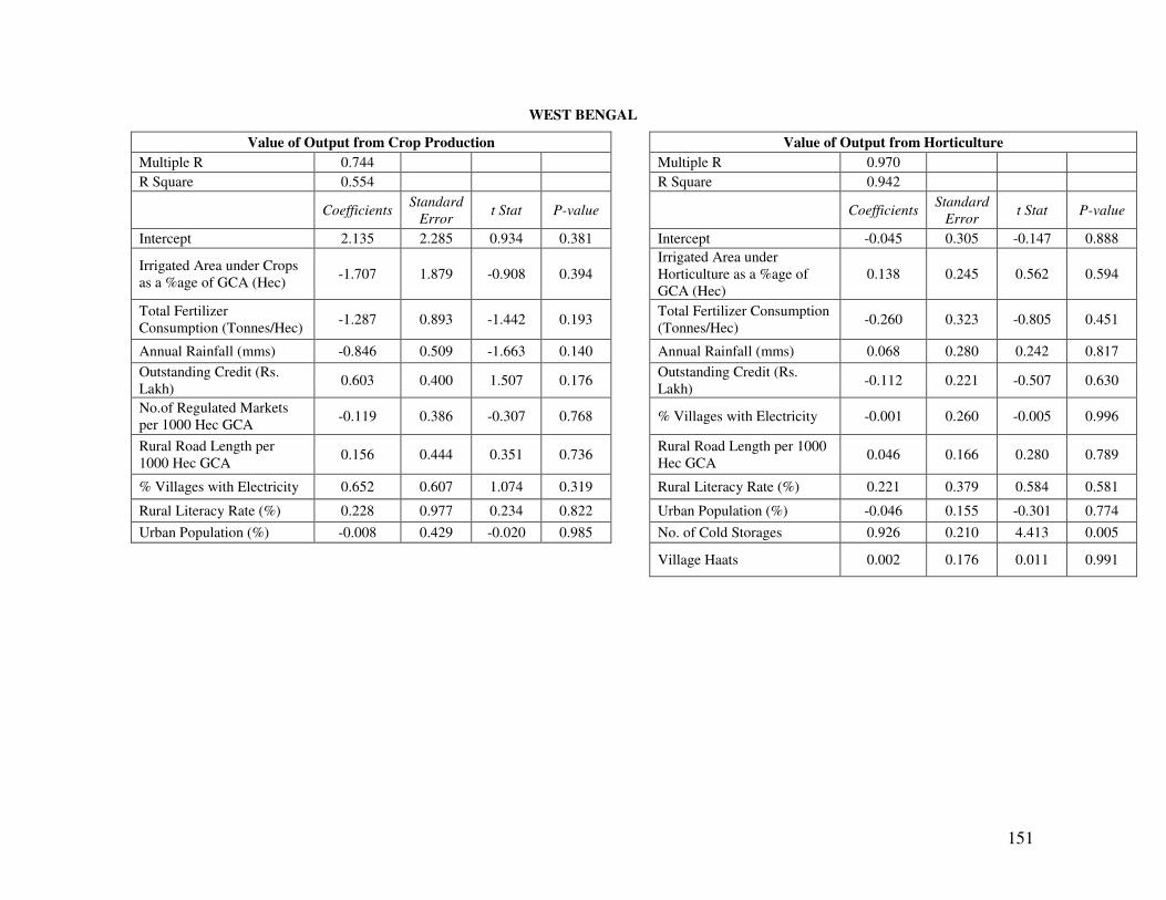
151
WEST BENGAL
Value of Output from Crop Production Value of Output from Horticulture
Multiple R 0.744 Multiple R 0.970
R Square 0.554 R Square 0.942
Coefficients Standard
Error t Stat P-value Coefficients
Standard
Error t Stat P-value
Intercept 2.135 2.285 0.934 0.381 Intercept -0.045 0.305 -0.147 0.888
Irrigated Area under Crops
as a %age of GCA (Hec) -1.707 1.879 -0.908 0.394
Irrigated Area under
Horticulture as a %age of
GCA (Hec)
0.138 0.245 0.562 0.594
Total Fertilizer
Consumption (Tonnes/Hec) -1.287 0.893 -1.442 0.193
Total Fertilizer Consumption
(Tonnes/Hec) -0.260 0.323 -0.805 0.451
Annual Rainfall (mms) -0.846 0.509 -1.663 0.140 Annual Rainfall (mms) 0.068 0.280 0.242 0.817
Outstanding Credit (Rs.
Lakh) 0.603 0.400 1.507 0.176
Outstanding Credit (Rs.
Lakh) -0.112 0.221 -0.507 0.630
No.of Regulated Markets
per 1000 Hec GCA -0.119 0.386 -0.307 0.768 % Villages with Electricity -0.001 0.260 -0.005 0.996
Rural Road Length per
1000 Hec GCA 0.156 0.444 0.351 0.736
Rural Road Length per 1000
Hec GCA 0.046 0.166 0.280 0.789
% Villages with Electricity 0.652 0.607 1.074 0.319 Rural Literacy Rate (%) 0.221 0.379 0.584 0.581
Rural Literacy Rate (%) 0.228 0.977 0.234 0.822 Urban Population (%) -0.046 0.155 -0.301 0.774
Urban Population (%) -0.008 0.429 -0.020 0.985 No. of Cold Storages 0.926 0.210 4.413 0.005
Village Haats 0.002 0.176 0.011 0.991

152
Value of Output from Livestock Value of Output from Forestry
Multiple R 0.952 Multiple R 0.966
R Square 0.907 R Square 0.933
Coefficients Standard
Error t Stat P-value
Coefficie
nts
Standard
Error t Stat P-value
Intercept 0.121 0.313 0.387 0.710 Intercept 0.377 0.194 1.949 0.083
Annual Rainfall (mms) 0.189 0.162 1.170 0.280 Annual Rainfall (mms) 0.516 0.132 3.923 0.003
Outstanding Credit (Rs. Lakh) 0.345 0.308 1.121 0.299 Outstanding Credit (Rs. Lakh) 0.359 0.146 2.468 0.036
% Villages with Electricity -0.060 0.227 -0.265 0.798 Rural Road Length per 1000
Hec GCA 0.452 0.125 3.628 0.006
Rural Road Length per 1000
Hec GCA -0.184 0.177 -1.042 0.332 Rural Literacy Rate (%) -1.346 0.279 -4.815 0.001
Rural Literacy Rate (%) -0.055 0.299 -0.184 0.859 Urban Population (%) 0.207 0.119 1.741 0.116
Urban Population (%) -0.102 0.150 -0.676 0.521 Village Haats 0.380 0.148 2.568 0.030
Village Haats 0.025 0.225 0.113 0.913 Forest Protection Committees 0.576 0.103 5.603 0.000
%age of Vetrinary Service
Establishments 0.620 0.289 2.146 0.069
Grazing & Pasture Land as a
%age of Reported Area 0.151 0.198 0.761 0.472
Value of Output from Fisheries
Multiple R 0.921
R Square 0.848
Coefficients Standard
Error t Stat P-value
Intercept -0.169 0.338 -0.501 0.630
Annual Rainfall (mms) 0.112 0.200 0.560 0.591
Outstanding Credit (Rs. Lakh) 0.790 0.206 3.836 0.005
% Villages with Electricity 0.018 0.229 0.080 0.938
Rural Road Length per 1000 Hec GCA 0.035 0.181 0.193 0.852
Rural Literacy Rate (%) -0.094 0.367 -0.256 0.805
Urban Population (%) -0.004 0.175 -0.024 0.982
No. of Cold Storages -0.196 0.155 -1.266 0.241
Village Haats 0.239 0.206 1.158 0.280
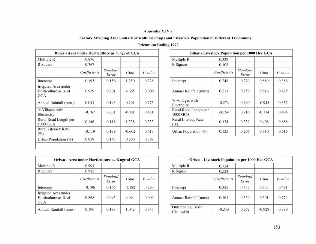
153
Appendix A.IV.2
Factors Affecting Area under Horticultural Crops and Livestock Population in Different Trienniums
Triennium Ending 1972
Bihar - Area under Horticulture as %age of GCA Bihar - Livestock Population per 1000 Hec GCA
Multiple R 0.876 Multiple R 0.329
R Square 0.767 R Square 0.108
Coefficients Standard
Error t Stat P-value Coefficients
Standard
Error t Stat P-value
Intercept 0.195 0.156 1.250 0.228 Intercept 0.248 0.279 0.889 0.386
Irrigated Area under
Horticulture as % of
GCA
0.939 0.201 4.665 0.000 Annual Rainfall (mms) 0.211 0.259 0.816 0.425
Annual Rainfall (mms) 0.041 0.143 0.291 0.775 % Villages with
Electricity -0.274 0.290 -0.945 0.357
% Villages with
Electricity -0.167 0.231 -0.720 0.481
Rural Road Length per
1000 GCA -0.154 0.216 -0.714 0.484
Rural Road Length per
1000 GCA 0.146 0.118 1.238 0.233
Rural Literacy Rate
(%) 0.134 0.329 0.408 0.688
Rural Literacy Rate
(%) -0.119 0.179 -0.662 0.517 Urban Population (%) 0.135 0.266 0.510 0.616
Urban Population (%) 0.038 0.145 0.260 0.798
Orissa - Area under Horticulture as %age of GCA Orissa - Livestock Population per 1000 Hec GCA
Multiple R 0.991 Multiple R 0.724
R Square 0.982 R Square 0.524
Coefficients Standard
Error t Stat P-value Coefficients
Standard
Error t Stat P-value
Intercept -0.196 0.166 -1.182 0.290 Intercept 0.335 0.457 0.733 0.491
Irrigated Area under
Horticulture as % of
GCA
0.868 0.095 9.094 0.000 Annual Rainfall (mms) 0.161 0.534 0.301 0.774
Annual Rainfall (mms) 0.196 0.188 1.042 0.345 Outstanding Credit
(Rs. Lakh) -0.243 0.262 -0.928 0.389
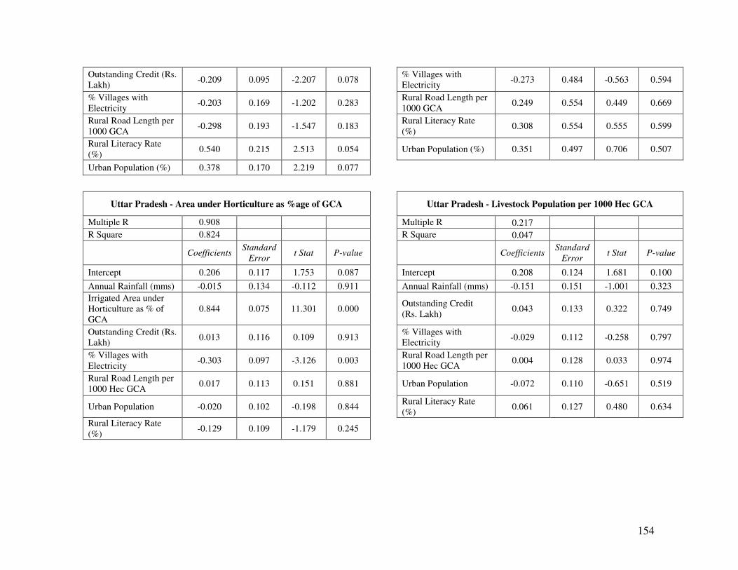
154
Outstanding Credit (Rs.
Lakh) -0.209 0.095 -2.207 0.078
% Villages with
Electricity -0.273 0.484 -0.563 0.594
% Villages with
Electricity -0.203 0.169 -1.202 0.283
Rural Road Length per
1000 GCA 0.249 0.554 0.449 0.669
Rural Road Length per
1000 GCA -0.298 0.193 -1.547 0.183
Rural Literacy Rate
(%) 0.308 0.554 0.555 0.599
Rural Literacy Rate
(%) 0.540 0.215 2.513 0.054 Urban Population (%) 0.351 0.497 0.706 0.507
Urban Population (%) 0.378 0.170 2.219 0.077
Uttar Pradesh - Area under Horticulture as %age of GCA Uttar Pradesh - Livestock Population per 1000 Hec GCA
Multiple R 0.908 Multiple R 0.217
R Square 0.824 R Square 0.047
Coefficients Standard
Error t Stat P-value Coefficients
Standard
Error t Stat P-value
Intercept 0.206 0.117 1.753 0.087 Intercept 0.208 0.124 1.681 0.100
Annual Rainfall (mms) -0.015 0.134 -0.112 0.911 Annual Rainfall (mms) -0.151 0.151 -1.001 0.323
Irrigated Area under
Horticulture as % of
GCA
0.844 0.075 11.301 0.000 Outstanding Credit
(Rs. Lakh) 0.043 0.133 0.322 0.749
Outstanding Credit (Rs.
Lakh) 0.013 0.116 0.109 0.913
% Villages with
Electricity -0.029 0.112 -0.258 0.797
% Villages with
Electricity -0.303 0.097 -3.126 0.003
Rural Road Length per
1000 Hec GCA 0.004 0.128 0.033 0.974
Rural Road Length per
1000 Hec GCA 0.017 0.113 0.151 0.881 Urban Population -0.072 0.110 -0.651 0.519
Urban Population -0.020 0.102 -0.198 0.844 Rural Literacy Rate
(%) 0.061 0.127 0.480 0.634
Rural Literacy Rate
(%) -0.129 0.109 -1.179 0.245
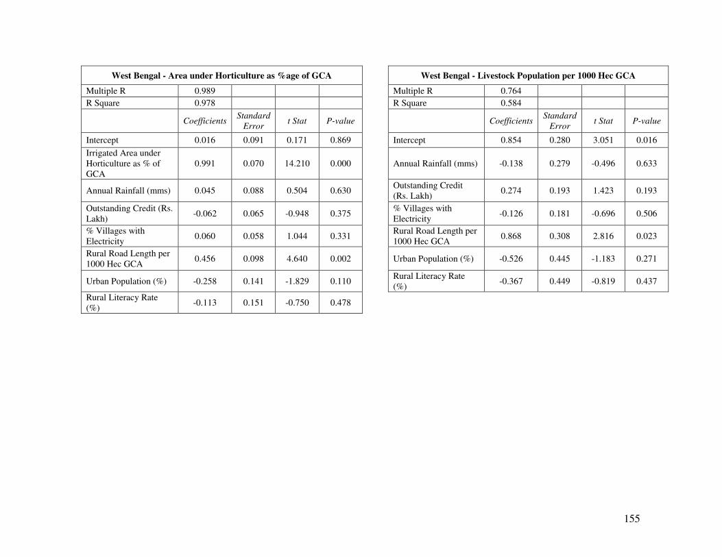
155
West Bengal - Area under Horticulture as %age of GCA West Bengal - Livestock Population per 1000 Hec GCA
Multiple R 0.989 Multiple R 0.764
R Square 0.978 R Square 0.584
Coefficients Standard
Error t Stat P-value Coefficients
Standard
Error t Stat P-value
Intercept 0.016 0.091 0.171 0.869 Intercept 0.854 0.280 3.051 0.016
Irrigated Area under
Horticulture as % of
GCA
0.991 0.070 14.210 0.000 Annual Rainfall (mms) -0.138 0.279 -0.496 0.633
Annual Rainfall (mms) 0.045 0.088 0.504 0.630 Outstanding Credit
(Rs. Lakh) 0.274 0.193 1.423 0.193
Outstanding Credit (Rs.
Lakh) -0.062 0.065 -0.948 0.375
% Villages with
Electricity -0.126 0.181 -0.696 0.506
% Villages with
Electricity 0.060 0.058 1.044 0.331
Rural Road Length per
1000 Hec GCA 0.868 0.308 2.816 0.023
Rural Road Length per
1000 Hec GCA 0.456 0.098 4.640 0.002 Urban Population (%) -0.526 0.445 -1.183 0.271
Urban Population (%) -0.258 0.141 -1.829 0.110 Rural Literacy Rate
(%) -0.367 0.449 -0.819 0.437
Rural Literacy Rate
(%) -0.113 0.151 -0.750 0.478
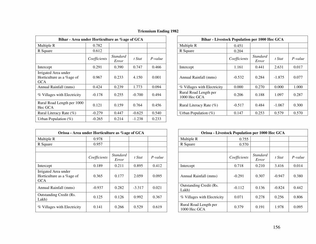
156
Triennium Ending 1982
Bihar - Area under Horticulture as %age of GCA Bihar - Livestock Population per 1000 Hec GCA
Multiple R 0.782 Multiple R 0.451
R Square 0.612 R Square 0.204
Coefficients Standard
Error t Stat P-value Coefficients
Standard
Error t Stat P-value
Intercept 0.291 0.390 0.747 0.466 Intercept 1.161 0.441 2.631 0.017
Irrigated Area under
Horticulture as a %age of
GCA
0.967 0.233 4.150 0.001 Annual Rainfall (mms) -0.532 0.284 -1.875 0.077
Annual Rainfall (mms) 0.424 0.239 1.773 0.094 % Villages with Electricity 0.000 0.270 0.000 1.000
% Villages with Electricity -0.178 0.255 -0.700 0.494 Rural Road Length per
1000 Hec GCA 0.206 0.188 1.097 0.287
Rural Road Length per 1000
Hec GCA 0.121 0.159 0.764 0.456 Rural Literacy Rate (%) -0.517 0.484 -1.067 0.300
Rural Literacy Rate (%) -0.279 0.447 -0.625 0.540 Urban Population (%) 0.147 0.253 0.579 0.570
Urban Population (%) -0.265 0.214 -1.238 0.233
Orissa - Area under Horticulture as %age of GCA Orissa - Livestock Population per 1000 Hec GCA
Multiple R 0.978 Multiple R 0.755
R Square 0.957 R Square 0.570
Coefficients Standard
Error t Stat P-value Coefficients
Standard
Error t Stat P-value
Intercept 0.189 0.211 0.895 0.412 Intercept 0.718 0.210 3.416 0.014
Irrigated Area under
Horticulture as a %age of
GCA
0.365 0.177 2.059 0.095 Annual Rainfall (mms) -0.291 0.307 -0.947 0.380
Annual Rainfall (mms) -0.937 0.282 -3.317 0.021 Outstanding Credit (Rs.
Lakh) -0.112 0.136 -0.824 0.442
Outstanding Credit (Rs.
Lakh) 0.125 0.126 0.992 0.367 % Villages with Electricity 0.071 0.278 0.256 0.806
% Villages with Electricity 0.141 0.266 0.529 0.619 Rural Road Length per
1000 Hec GCA 0.379 0.191 1.978 0.095
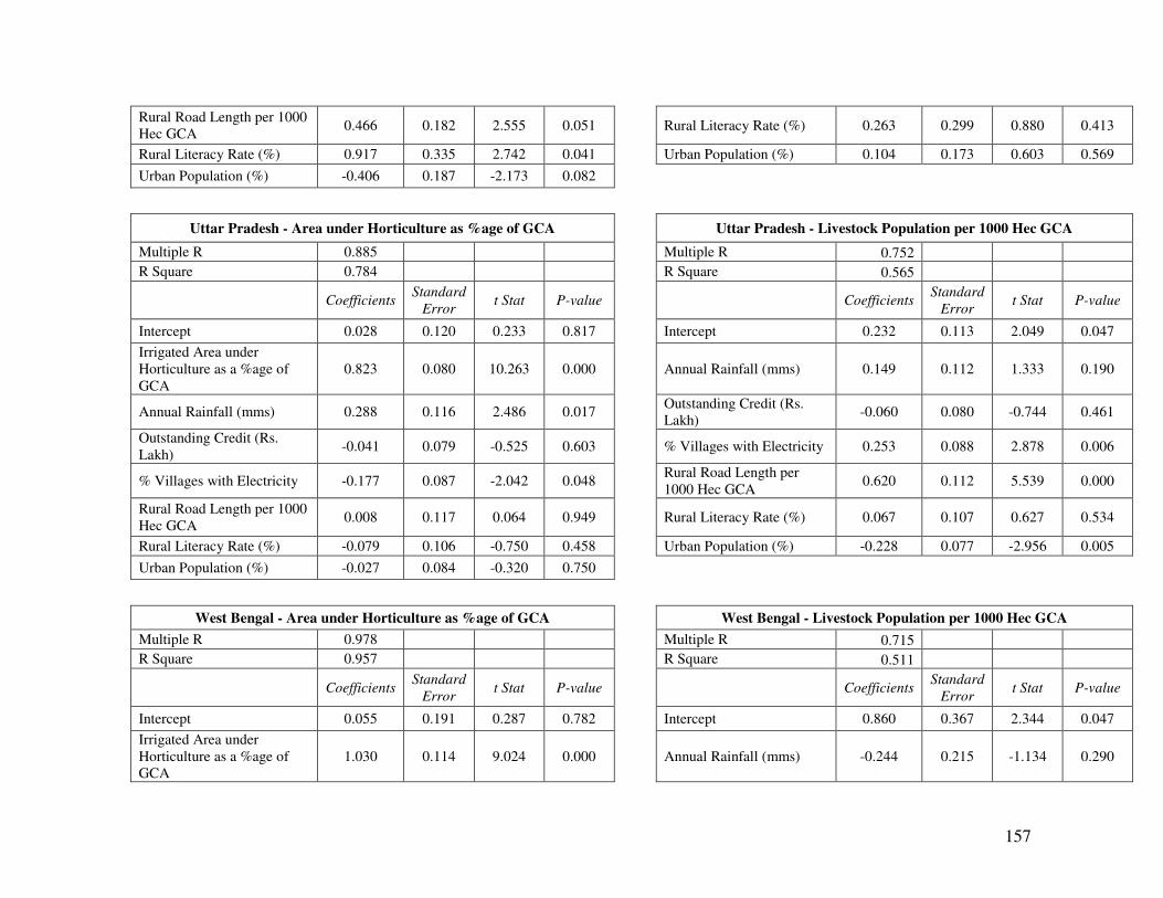
157
Rural Road Length per 1000
Hec GCA 0.466 0.182 2.555 0.051 Rural Literacy Rate (%) 0.263 0.299 0.880 0.413
Rural Literacy Rate (%) 0.917 0.335 2.742 0.041 Urban Population (%) 0.104 0.173 0.603 0.569
Urban Population (%) -0.406 0.187 -2.173 0.082
Uttar Pradesh - Area under Horticulture as %age of GCA Uttar Pradesh - Livestock Population per 1000 Hec GCA
Multiple R 0.885 Multiple R 0.752
R Square 0.784 R Square 0.565
Coefficients Standard
Error t Stat P-value Coefficients
Standard
Error t Stat P-value
Intercept 0.028 0.120 0.233 0.817 Intercept 0.232 0.113 2.049 0.047
Irrigated Area under
Horticulture as a %age of
GCA
0.823 0.080 10.263 0.000 Annual Rainfall (mms) 0.149 0.112 1.333 0.190
Annual Rainfall (mms) 0.288 0.116 2.486 0.017 Outstanding Credit (Rs.
Lakh) -0.060 0.080 -0.744 0.461
Outstanding Credit (Rs.
Lakh) -0.041 0.079 -0.525 0.603 % Villages with Electricity 0.253 0.088 2.878 0.006
% Villages with Electricity -0.177 0.087 -2.042 0.048 Rural Road Length per
1000 Hec GCA 0.620 0.112 5.539 0.000
Rural Road Length per 1000
Hec GCA 0.008 0.117 0.064 0.949 Rural Literacy Rate (%) 0.067 0.107 0.627 0.534
Rural Literacy Rate (%) -0.079 0.106 -0.750 0.458 Urban Population (%) -0.228 0.077 -2.956 0.005
Urban Population (%) -0.027 0.084 -0.320 0.750
West Bengal - Area under Horticulture as %age of GCA West Bengal - Livestock Population per 1000 Hec GCA
Multiple R 0.978 Multiple R 0.715
R Square 0.957 R Square 0.511
Coefficients Standard
Error t Stat P-value Coefficients
Standard
Error t Stat P-value
Intercept 0.055 0.191 0.287 0.782 Intercept 0.860 0.367 2.344 0.047
Irrigated Area under
Horticulture as a %age of
GCA
1.030 0.114 9.024 0.000 Annual Rainfall (mms) -0.244 0.215 -1.134 0.290
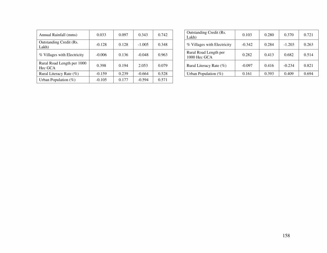
158
Annual Rainfall (mms) 0.033 0.097 0.343 0.742 Outstanding Credit (Rs.
Lakh) 0.103 0.280 0.370 0.721
Outstanding Credit (Rs.
Lakh) -0.128 0.128 -1.005 0.348 % Villages with Electricity -0.342 0.284 -1.203 0.263
% Villages with Electricity -0.006 0.136 -0.048 0.963 Rural Road Length per
1000 Hec GCA 0.282 0.413 0.682 0.514
Rural Road Length per 1000
Hec GCA 0.398 0.194 2.053 0.079 Rural Literacy Rate (%) -0.097 0.416 -0.234 0.821
Rural Literacy Rate (%) -0.159 0.239 -0.664 0.528 Urban Population (%) 0.161 0.393 0.409 0.694
Urban Population (%) -0.105 0.177 -0.594 0.571
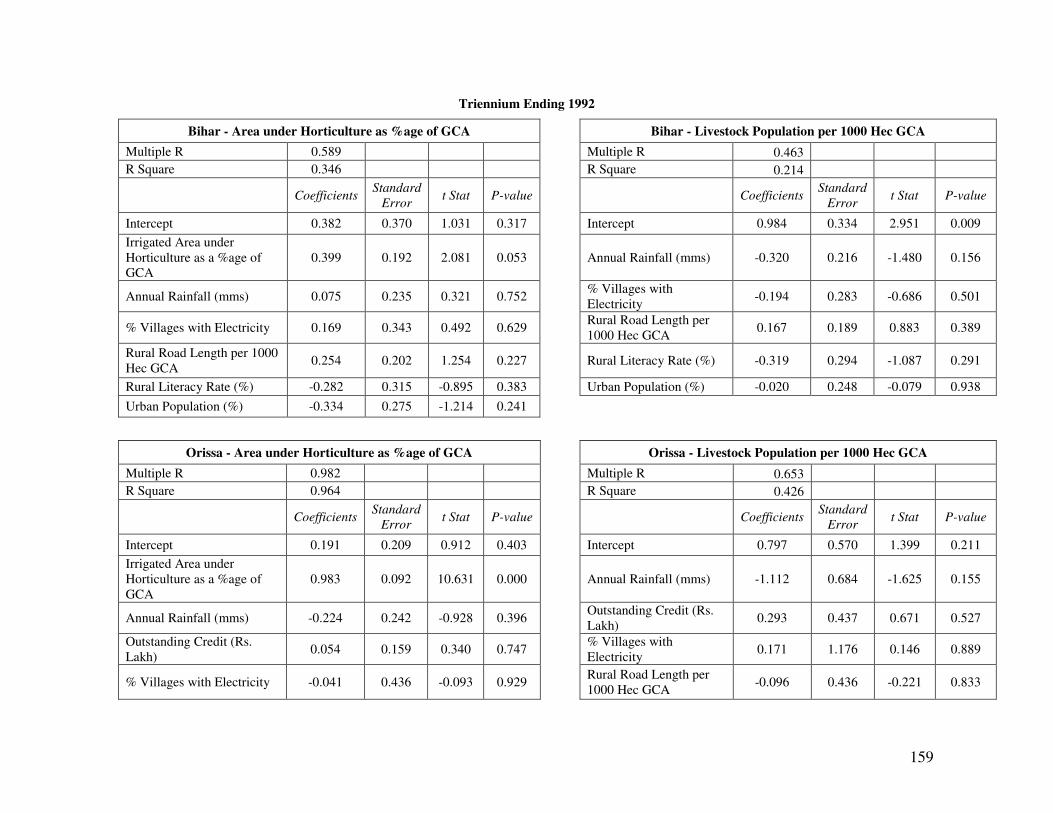
159
Triennium Ending 1992
Bihar - Area under Horticulture as %age of GCA Bihar - Livestock Population per 1000 Hec GCA
Multiple R 0.589 Multiple R 0.463
R Square 0.346 R Square 0.214
Coefficients Standard
Error t Stat P-value Coefficients
Standard
Error t Stat P-value
Intercept 0.382 0.370 1.031 0.317 Intercept 0.984 0.334 2.951 0.009
Irrigated Area under
Horticulture as a %age of
GCA
0.399 0.192 2.081 0.053 Annual Rainfall (mms) -0.320 0.216 -1.480 0.156
Annual Rainfall (mms) 0.075 0.235 0.321 0.752 % Villages with
Electricity -0.194 0.283 -0.686 0.501
% Villages with Electricity 0.169 0.343 0.492 0.629 Rural Road Length per
1000 Hec GCA 0.167 0.189 0.883 0.389
Rural Road Length per 1000
Hec GCA 0.254 0.202 1.254 0.227 Rural Literacy Rate (%) -0.319 0.294 -1.087 0.291
Rural Literacy Rate (%) -0.282 0.315 -0.895 0.383 Urban Population (%) -0.020 0.248 -0.079 0.938
Urban Population (%) -0.334 0.275 -1.214 0.241
Orissa - Area under Horticulture as %age of GCA Orissa - Livestock Population per 1000 Hec GCA
Multiple R 0.982 Multiple R 0.653
R Square 0.964 R Square 0.426
Coefficients Standard
Error t Stat P-value Coefficients
Standard
Error t Stat P-value
Intercept 0.191 0.209 0.912 0.403 Intercept 0.797 0.570 1.399 0.211
Irrigated Area under
Horticulture as a %age of
GCA
0.983 0.092 10.631 0.000 Annual Rainfall (mms) -1.112 0.684 -1.625 0.155
Annual Rainfall (mms) -0.224 0.242 -0.928 0.396 Outstanding Credit (Rs.
Lakh) 0.293 0.437 0.671 0.527
Outstanding Credit (Rs.
Lakh) 0.054 0.159 0.340 0.747
% Villages with
Electricity 0.171 1.176 0.146 0.889
% Villages with Electricity -0.041 0.436 -0.093 0.929 Rural Road Length per
1000 Hec GCA -0.096 0.436 -0.221 0.833
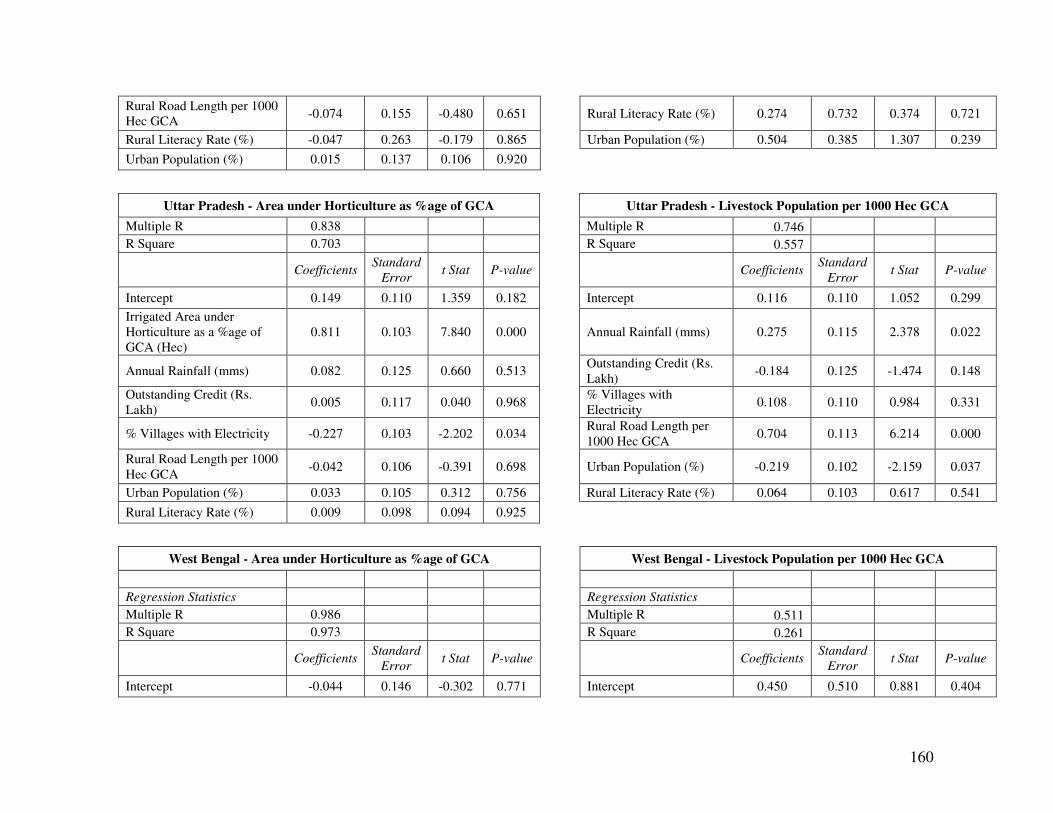
160
Rural Road Length per 1000
Hec GCA -0.074 0.155 -0.480 0.651 Rural Literacy Rate (%) 0.274 0.732 0.374 0.721
Rural Literacy Rate (%) -0.047 0.263 -0.179 0.865 Urban Population (%) 0.504 0.385 1.307 0.239
Urban Population (%) 0.015 0.137 0.106 0.920
Uttar Pradesh - Area under Horticulture as %age of GCA Uttar Pradesh - Livestock Population per 1000 Hec GCA
Multiple R 0.838 Multiple R 0.746
R Square 0.703 R Square 0.557
Coefficients Standard
Error t Stat P-value Coefficients
Standard
Error t Stat P-value
Intercept 0.149 0.110 1.359 0.182 Intercept 0.116 0.110 1.052 0.299
Irrigated Area under
Horticulture as a %age of
GCA (Hec)
0.811 0.103 7.840 0.000 Annual Rainfall (mms) 0.275 0.115 2.378 0.022
Annual Rainfall (mms) 0.082 0.125 0.660 0.513 Outstanding Credit (Rs.
Lakh) -0.184 0.125 -1.474 0.148
Outstanding Credit (Rs.
Lakh) 0.005 0.117 0.040 0.968
% Villages with
Electricity 0.108 0.110 0.984 0.331
% Villages with Electricity -0.227 0.103 -2.202 0.034 Rural Road Length per
1000 Hec GCA 0.704 0.113 6.214 0.000
Rural Road Length per 1000
Hec GCA -0.042 0.106 -0.391 0.698 Urban Population (%) -0.219 0.102 -2.159 0.037
Urban Population (%) 0.033 0.105 0.312 0.756 Rural Literacy Rate (%) 0.064 0.103 0.617 0.541
Rural Literacy Rate (%) 0.009 0.098 0.094 0.925
West Bengal - Area under Horticulture as %age of GCA West Bengal - Livestock Population per 1000 Hec GCA
Regression Statistics Regression Statistics
Multiple R 0.986 Multiple R 0.511
R Square 0.973 R Square 0.261
Coefficients Standard
Error t Stat P-value Coefficients
Standard
Error t Stat P-value
Intercept -0.044 0.146 -0.302 0.771 Intercept 0.450 0.510 0.881 0.404

161
Irrigated Area under
Horticulture as a %age of
GCA (Hec)
0.931 0.084 11.105 0.000 Annual Rainfall (mms) -0.187 0.352 -0.532 0.609
Annual Rainfall (mms) 0.063 0.101 0.622 0.554 Outstanding Credit (Rs.
Lakh) 0.166 0.434 0.382 0.713
Outstanding Credit (Rs.
Lakh) -0.122 0.124 -0.981 0.359
% Villages with
Electricity 0.317 0.424 0.746 0.477
% Villages with Electricity 0.044 0.124 0.353 0.735 Rural Road Length per
1000 Hec GCA 0.389 0.328 1.184 0.271
Rural Road Length per 1000
Hec GCA 0.068 0.101 0.677 0.520 Urban Population (%) -0.546 0.364 -1.499 0.172
Urban Population (%) 0.142 0.124 1.147 0.289 Rural Literacy Rate (%) 0.094 0.654 0.144 0.889
Rural Literacy Rate (%) -0.142 0.188 -0.757 0.474
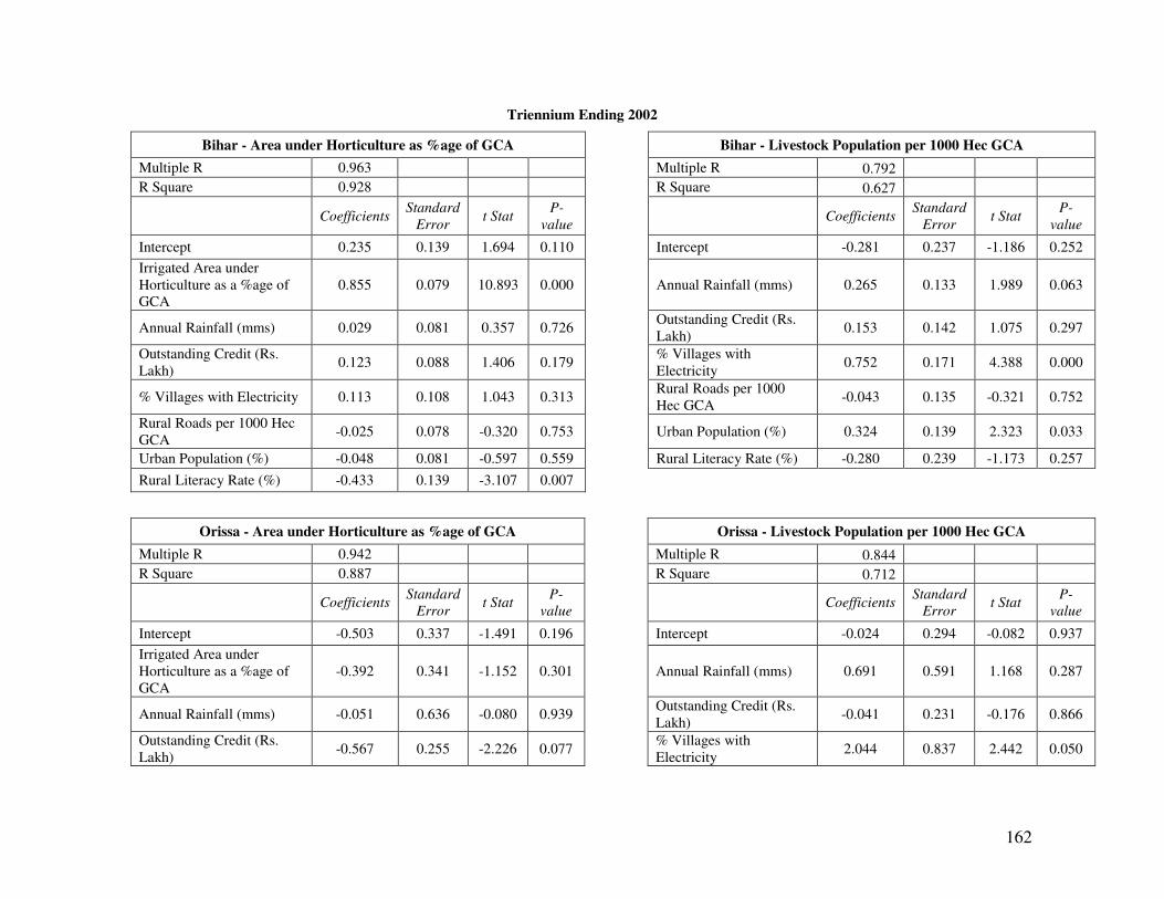
162
Triennium Ending 2002
Bihar - Area under Horticulture as %age of GCA Bihar - Livestock Population per 1000 Hec GCA
Multiple R 0.963 Multiple R 0.792
R Square 0.928 R Square 0.627
Coefficients Standard
Error t Stat
P-
value Coefficients
Standard
Error t Stat
P-
value
Intercept 0.235 0.139 1.694 0.110 Intercept -0.281 0.237 -1.186 0.252
Irrigated Area under
Horticulture as a %age of
GCA
0.855 0.079 10.893 0.000 Annual Rainfall (mms) 0.265 0.133 1.989 0.063
Annual Rainfall (mms) 0.029 0.081 0.357 0.726 Outstanding Credit (Rs.
Lakh) 0.153 0.142 1.075 0.297
Outstanding Credit (Rs.
Lakh) 0.123 0.088 1.406 0.179
% Villages with
Electricity 0.752 0.171 4.388 0.000
% Villages with Electricity 0.113 0.108 1.043 0.313 Rural Roads per 1000
Hec GCA -0.043 0.135 -0.321 0.752
Rural Roads per 1000 Hec
GCA -0.025 0.078 -0.320 0.753 Urban Population (%) 0.324 0.139 2.323 0.033
Urban Population (%) -0.048 0.081 -0.597 0.559 Rural Literacy Rate (%) -0.280 0.239 -1.173 0.257
Rural Literacy Rate (%) -0.433 0.139 -3.107 0.007
Orissa - Area under Horticulture as %age of GCA Orissa - Livestock Population per 1000 Hec GCA
Multiple R 0.942 Multiple R 0.844
R Square 0.887 R Square 0.712
Coefficients Standard
Error t Stat
P-
value Coefficients
Standard
Error t Stat
P-
value
Intercept -0.503 0.337 -1.491 0.196 Intercept -0.024 0.294 -0.082 0.937
Irrigated Area under
Horticulture as a %age of
GCA
-0.392 0.341 -1.152 0.301 Annual Rainfall (mms) 0.691 0.591 1.168 0.287
Annual Rainfall (mms) -0.051 0.636 -0.080 0.939 Outstanding Credit (Rs.
Lakh) -0.041 0.231 -0.176 0.866
Outstanding Credit (Rs.
Lakh) -0.567 0.255 -2.226 0.077
% Villages with
Electricity 2.044 0.837 2.442 0.050
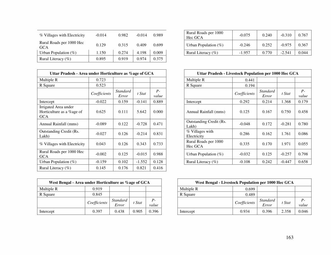
163
% Villages with Electricity -0.014 0.982 -0.014 0.989 Rural Roads per 1000
Hec GCA -0.075 0.240 -0.310 0.767
Rural Roads per 1000 Hec
GCA 0.129 0.315 0.409 0.699 Urban Population (%) -0.246 0.252 -0.975 0.367
Urban Population (%) 1.150 0.274 4.198 0.009 Rural Literacy (%) -1.957 0.770 -2.541 0.044
Rural Literacy (%) 0.895 0.919 0.974 0.375
Uttar Pradesh - Area under Horticulture as %age of GCA Uttar Pradesh - Livestock Population per 1000 Hec GCA
Multiple R 0.723 Multiple R 0.441
R Square 0.523 R Square 0.194
Coefficients Standard
Error t Stat
P-
value Coefficients
Standard
Error t Stat
P-
value
Intercept -0.022 0.159 -0.141 0.889 Intercept 0.292 0.214 1.368 0.179
Irrigated Area under
Horticulture as a %age of
GCA
0.625 0.111 5.642 0.000 Annual Rainfall (mms) 0.125 0.167 0.750 0.458
Annual Rainfall (mms) -0.089 0.122 -0.728 0.471 Outstanding Credit (Rs.
Lakh) -0.048 0.172 -0.281 0.780
Outstanding Credit (Rs.
Lakh) -0.027 0.126 -0.214 0.831
% Villages with
Electricity 0.286 0.162 1.761 0.086
% Villages with Electricity 0.043 0.126 0.343 0.733 Rural Roads per 1000
Hec GCA 0.335 0.170 1.971 0.055
Rural Roads per 1000 Hec
GCA -0.002 0.125 -0.015 0.988 Urban Population (%) -0.032 0.125 -0.257 0.798
Urban Population (%) -0.159 0.102 -1.552 0.128 Rural Literacy (%) -0.108 0.242 -0.447 0.658
Rural Literacy (%) 0.145 0.176 0.821 0.416
West Bengal - Area under Horticulture as %age of GCA West Bengal - Livestock Population per 1000 Hec GCA
Multiple R 0.919 Multiple R 0.699
R Square 0.845 R Square 0.489
Coefficients Standard
Error t Stat
P-
value Coefficients
Standard
Error t Stat
P-
value
Intercept 0.397 0.438 0.905 0.396 Intercept 0.934 0.396 2.358 0.046
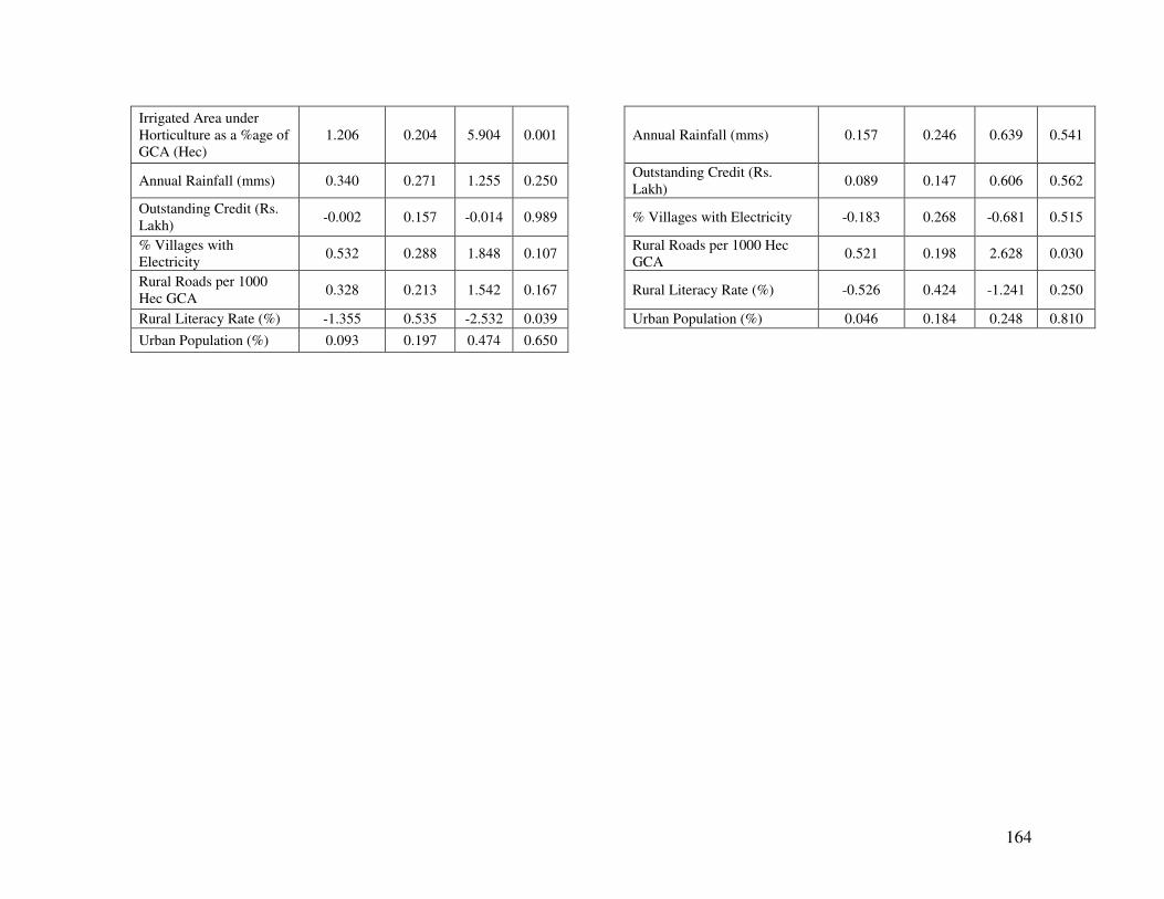
164
Irrigated Area under
Horticulture as a %age of
GCA (Hec)
1.206 0.204 5.904 0.001 Annual Rainfall (mms) 0.157 0.246 0.639 0.541
Annual Rainfall (mms) 0.340 0.271 1.255 0.250 Outstanding Credit (Rs.
Lakh) 0.089 0.147 0.606 0.562
Outstanding Credit (Rs.
Lakh) -0.002 0.157 -0.014 0.989 % Villages with Electricity -0.183 0.268 -0.681 0.515
% Villages with
Electricity 0.532 0.288 1.848 0.107
Rural Roads per 1000 Hec
GCA 0.521 0.198 2.628 0.030
Rural Roads per 1000
Hec GCA 0.328 0.213 1.542 0.167 Rural Literacy Rate (%) -0.526 0.424 -1.241 0.250
Rural Literacy Rate (%) -1.355 0.535 -2.532 0.039 Urban Population (%) 0.046 0.184 0.248 0.810
Urban Population (%) 0.093 0.197 0.474 0.650
165
CHAPTER V
CONCLUSIONS AND POLICY IMPLICATIONS
This study analyzed the trends and patterns of agricultural diversification and
related development in the Eastern states of India comprising the states of Bihar, Uttar
Pradesh, Jharkhand, Orissa and West Bengal. The main objectives of this study were to
analyse the trends and patterns of rural diversification, including both horizontal and
vertical diversification in eastern India, to analyse the constraints and potentials of
diversified rural growth in the different eastern states, considering various agro-climatic,
socio-economic, technological, infrastructural, institutional and policy factors, to analyse
the various economic aspects including production, profitability, equity and viability of
small and marginal farms in the context of diversification and lastly to identify potential
sources and suggest appropriate strategies and policies for accelerated and diversified
agricultural growth as well as sustainability of small/marginal farms in these regions.
In India the share of GDP from agriculture declined from 35% in 1980-81 to
18.11% in 2007-08, while that of non-agriculture increased from 64.30% to 81.89% in
the same period. The eastern states followed the same trend as that of India. Further, the
share of GSDP from agriculture and allied activities was relatively higher in Uttar
Pradesh (29.40%) followed by Bihar (25.34%), Orissa (22.97%), West Bengal (21.39%)
and lastly Jharkhand (9.49%).
Within the agriculture & allied activities sector the share of agriculture including
livestock in recent years was highest in Uttar Pradesh (95.2%) followed by Bihar, West
Bengal, Orissa and Jharkhand (approximately 80%). The share of forestry & logging was
highest in Jharkhand (12.08%), followed by Orissa and Bihar (approximately 7%). In
Uttar Pradesh and West Bengal the shares were very low (approximately 3%). The share
of fisheries was highest in West Bengal (10.23%) followed by Orissa and Bihar
(approximately 5%). The fisheries sector showed very low shares in Jharkhand and Uttar
Pradesh i.e., 3.93% and 1.28% respectively.
There has been a significant change in the cropping pattern in the past few
decades. In India as a whole as well in all the eastern states the area share of cereals in the
GCA has been highest amongst other crops from 1970-71 to 2007-08. It was also

166
observed that the area devoted to food grains was much higher in all the eastern states
compared to horticultural crops. The proportionate area under horticultural crops was
relatively high only in West Bengal and Bihar.
Cropping pattern in each state was compared between 1999-2000 and 2006-07 by
using the index of crop diversification formulated by Bhatia (1965). It was seen that crop
diversification had reduced from their 1999-2000 levels in the state of Bihar, Orissa and
Jharkhand, while it increased slightly in Uttar Pradesh and a lot in West Bengal. Further,
from the Simpson’s index of crop diversification it was seen in Bihar crop diversification
away from food grains increased since 1970-71 but after 2000-01 it showed a decline. In
Jharkhand it decreased. In Orissa crop diversification away from food grains reduced
especially since 1995-96. In Uttar Pradesh crop diversification away from food grains
increased slightly, whereas in West Bengal crop diversification away from food grains
increased tremendously.
There have also been significant changes in the relative shares of various crops in
the gross value of crop output from agriculture (crop sector) in the past few decades. In
Bihar the share of food grains, especially pulses have shown a sizeable decline over the
years. The shares of other crops especially fruits & vegetables have increased and are
even more than cereal crops, thereby showing diversification towards fruits & vegetables
in Bihar. Jharkhand also shows diversification from cereals toward fruits & vegetables.
All other crops except fibre crops and condiments & spices have shown a marginal
increase in their shares. In Orissa the share of cereals and fruits & vegetables showed
significant increase from their 1980-81 levels. The share of condiments & spices showed
marginal increase, while the shares of pulses, oilseeds, fibre crops and sugarcane showed
a decline. In Uttar Pradesh cereal crops showed higher share compared to fruits &
vegetables and both their shares showed an increase over time. The shares of pulses and
oilseeds showed a decline whereas those of fibres and condiments & spices have shown a
marginal increase. In West Bengal the share of cereals declined over the years while
those of fruits & vegetables increased from their 1980-81 levels. The share of condiments
& spices showed marginal increase, while the rest of crops showed marginal decline. It
was seen from the analysis of cropping pattern and value of output of crops that though
area diversification away from food grains towards horticultural crops was significant
167
over the years in the eastern states but in terms of value of output, the share of
horticultural crops was very high compared to other crops in all the eastern states except
Uttar Pradesh. It is to be noted that Uttar Pradesh is one of the Green Revolution states
and hence cultivation of food grains is very important here.
The sector wise distribution of value of output in agriculture and allied activities
showed that in Bihar the share of livestock was highest (31.32%) followed closely by the
crop sector (excluding horticulture) (30.34%) and horticultural sector (28.77%). The
share of forestry and fisheries was very low (around 5%). In West Bengal the share of
crop sector was the highest (36.11%) followed closely by the horticulture (31.19%),
livestock (17.38%), fisheries (12.18%) and lastly forestry (3.14%). The pattern was
similar in Orissa and Jharkhand. In Uttar Pradesh the share of crop sector was the highest
(59.23%) followed by livestock (26.76%). The shares of horticulture, forestry and
fisheries were very low (less than 10%).
In all the eastern states a high proportion of fruits area was under mango. In West
Bengal, a high proportion of vegetables area was under cucurbits and brinjal. In Bihar
and Uttar Pradesh, it was under potato and in Orissa, it was under rabi vegetables.
Amongst livestock population in India sheep, followed by buffaloes and goats
showed a higher growth rate between the years 1992-93 and 2003-04 compared to cattle
whose growth rate showed a decline (-0.08%). The growth rate of cattle declined in all
the eastern states except West Bengal (0.99%). The growth rate of buffaloes was highest
in Uttar Pradesh (1.09%) while that of sheep was highest in Orissa (5.65%). The growth
rate of goats was highest in West Bengal (5.65%).
In all eastern states, the share of milk in the total value of livestock output was the
highest (approximately 50%) amongst all other livestock products. Its share was highest
in Uttar Pradesh (approximately 80%) followed by Jharkhand, Bihar, Orissa and West
Bengal. The shares have increased for all the eastern states except Jharkhand between
TE-2002 and TE-2006. The contribution of meat in the total value of livestock output
was the second highest after milk (approximately 17%). Its share was highest in West
Bengal (approximately 45%) followed by Orissa, Bihar, Uttar Pradesh and Jharkhand.
The shares have declined marginally for most eastern states except Uttar Pradesh and
Jharkhand between TE-2002 and TE-2006.
168
The major fish producing eastern states were West Bengal and Orissa. In India the
share of inland fish in the total value of output of fisheries increased from 48% to 52%
between TE-2002 and TE-2006 while the share of marine fisheries decreased from 52%
to 48% in the same period. In the states of Bihar and Uttar Pradesh and Jharkhand the
contribution of inland fisheries in total value output from fisheries was 100%. In Orissa,
the contribution of marine fisheries was more than inland fisheries whereas in West
Bengal it was just the opposite. Further the contribution of marine fisheries in both Orissa
and West Bengal declined while that of inland fisheries was increased.
The proportionate area under forestry to the total reported area, in India increased
marginally from 21.55% in 1970-71 to 22.99% in 2006-07. It declined in Bihar
(including Jharkhand) and Uttar Pradesh from around 16% to 6%. In Orissa it increased
from 32% to 37%, while in West Bengal it increased from 12.44 to 13.52% during the
same period.
The share of forestry & logging in the total value of output of agriculture and
allied activities showed a slight decline from 3.64% to 3.50% between TE – 2002 and TE
– 2006. The shares were highest in Jharkhand followed by Orissa, Bihar, West Bengal
and Uttar Pradesh. The shares showed marginal increase in the states of Bihar, Uttar
Pradesh and West Bengal, while in Orissa and Jharkhand they showed a marginal
decline. The share of fuel wood in the total value of output from forestry was the highest
(approximately 80%), followed by industrial wood and minor forest products (MFP)
(approximately 9%) in TE-2002 and TE-2006. The shares of fuel wood were highest in
Bihar (99%), Uttar Pradesh (96%), West Bengal (93%), Orissa (88%) and Jharkhand
(73%). The shares of Fuel Wood have increased in all eastern states except Jharkhand.
The shares of industrial wood and MFP have declined in all the eastern states except
Jharkhand where the share of MFP increased tremendously in between both periods.
In the employment sector, it was seen that the share of employed persons in
agriculture (usual principal status plus usual subsidiary status) in rural Bihar declined
from 84.3% in 1993-94 to 77.9% in 2004-05. At the same time non-agricultural
employment increased from 15.7% to 22.1%. In Orissa it declined from 80.9% to 69%
and non-agricultural employment increased from 19.1% to 31%. In Uttar Pradesh it
declined from 80% to 72.8% and non-agricultural employment increased from 20% to
169
27.2%. In West Bengal it declined marginally from 63.3% in 1993-94 to 62.7% in 2004-
05. At the same time non-agricultural employment increased marginally from 36.7% to
37.3%.
In 2002-03, amongst the various sources of household income, the average
income from crop cultivation was the highest (Rs. 969) followed by wage earnings other
than casual labour (Rs. 434), casual wage labour (Rs. 385) and dairy farming (Rs. 131).
The other sources, namely, fish farming and animal farming did not generate any income
but resulted in losses (income being negative). Out of the 5 states taken into
consideration, the average income generated from animal farming was found positive
only in case of West Bengal and Orissa, the average income being Rs.15 and Rs.3 per
month respectively. Out of the 5 states, the average income earned by households was
highest in West Bengal (Rs. 2079) followed by Jharkhand (Rs. 2069), Bihar (Rs.1810),
Uttar Pradesh (Rs.1633) and Orissa (Rs. 1062).
From the data on average income earned and average expenditure incurred in
2002-03 by farming households on a monthly basis, it was seen that for farming
households having less than 4 hectares of land, average income earned was less than their
average expenditure in all the eastern states. Hence their income was not enough to meet
the expenditure on consumption.
To understand non-farm diversification a set of regression exercises were done
with the dependent variable being rural non-farm workers and the independent variables
being urban population, rural literacy and wage rates. In the state of Bihar it was
observed that the rural non-farm workers showed a positive relation with urban
population and rural literacy rate whereas with respect to agricultural wage rates, the
relation was negative. For Jharkhand, the relationship with respect to urban population
and wage rates was same as that of Bihar, whereas with respect to rural literacy rate the
relationship was negative. In case of Orissa and Uttar Pradesh, the scenario was very
much similar.
Amongst agro-processing industries; it was the food processing industry which
provided greater share (in terms of GVA, employment and number of production units)
under organized sector whereas it was the non food industry which accounted for greater
share in case of unorganized sector. Out of the five states studied in this project; Uttar
170
Pradesh had the highest percentage share (13.40%) in the gross value added of food
processing industry in the organized sector for all the states in India, followed by West
Bengal with 2.07%. Bihar stood third with share of 1.22% followed by Orissa at 0.8%.
Jharkhand performed poorly with share of 0.28%. Taking employment in organized
sector into consideration, Uttar Pradesh again performed best where the percent share in
total employment was 11.46% followed by West Bengal with 4.43%. Share of Orissa in
case of employment was better (1.57%) than that of Bihar (0.88%). Jharkhand again
came last with percentage share of 0.15%. However, with respect to labour productivity
(which was GVA/Employment); Jharkhand stood first with productivity of 1.87 followed
by Bihar with productivity of 1.38. Uttar Pradesh stood third with productivity of 1.17
followed by Orissa with 1.10. West Bengal performed really badly with respect to labour
productivity. This implied that in this industry labour was most efficient in Jharkhand and
least efficient in West Bengal.
The share of agricultural vis-à-vis non-agricultural exports in the total exports
from India showed a declining trend since 1970-71. Only the already high shares of non-
agricultural exports are seen to be rising. Further, the growth rate of agricultural exports
between 1980-81 and 2008-09 has been 7.72% and amongst principal agricultural
commodities exported the growth rates have been highest for Sugar & Molasses
(11.47%) followed by Meat & Meat Preparations (10.30%), Rice (9.96%), Oil cakes
(9.14%), fruits (8.86%) and spices (8.60%).
All these above mentioned statistics do indicate that there was a positive trend
towards both horizontal as well as vertical diversification of the rural economy of eastern
India.
In the field survey agriculture and allied activities included the crop, livestock and
fisheries sectors only. The forestry sector was not observed. Within the crop sector, from
the field survey it was observed that sample farming households in the selected study
regions mainly cultivated cereals, pulses, oilseeds, vegetables, jute and sugarcane.
Cultivation of fruits and flowers was rarely observed. It was seen that cereals were
cultivated by majority households across all farm size categories in all the states. Further
cereals also occupied a large proportion of the gross cropped area in all the states. The
Simpson’s Index of Diversification (SID) was the highest in Orissa (0.25) followed by
171
Bihar (0.18), West Bengal (0.16), Uttar Pradesh (0.15), and Jharkhand (0.08). In the
states of Orissa, Bihar, West Bengal and Jharkhand the crop diversification away from
food grains was mainly towards oilseeds while in Uttar Pradesh it was mainly towards
sugarcane. Some diversification towards cultivation of vegetables was observed mainly
in the states of Orissa and West Bengal. It was also found that developed districts showed
greater crop diversification away from food grains towards non-food grain crops
compared to under developed districts except for Kishanganj in Bihar and Jalpaiguri in
West Bengal which showed diversification towards oilseeds and jute. From the SID
compared using both primary and secondary data it is seen that the state of Orissa showed
more diversification away from food grains and Jharkhand showed least diversification.
From the field survey data in the selected districts it was seen that small and
marginal farmers showed more horizontal diversification within the crop sector towards
high value crops such as oilseeds, sugarcane, jute and vegetables compared to the other
categories. Conversely, this category of farmers has shown comparatively lesser
horizontal diversification with the allied sectors such as livestock and fisheries compared
to the other farm sizes. The reasons for this is that, since high value crops gave higher
yields and earlier returns compared to food grains, small and marginal farmers tried to
maximize their returns from their small holdings by allocating more acreages to these
high value crops whereas large farmers tended to hedge their bets by devoting more area
towards food grains and also diversifying more within the allied sectors like livestock and
fisheries.
In all the selected five states, the developed districts showed higher yield levels
for most crops than the underdeveloped districts. It was also noticed that most crop yields
both for food grain crops and high value crops showed a positive relation with farm size.
Further, it was also seen that crop diversification towards high value crops mainly
vegetables and sugarcane suits the need of farmers especially small and marginal holders
as the yield levels of these crops are much higher compared to other crops and it was also
reported by farmers that the returns, especially from vegetables, were more regular and
earlier compared to food grains.
172
In all the five states the developed districts showed higher yield levels than the
underdeveloped districts. It was also noticed that most crop yields showed a positive
relation with farm size in all the five states surveyed.
From the pattern of livestock in the study regions it was seen that majority of the
sample farming households owned cattle. The highest proportion of cattle was seen in
West Bengal (70%) followed by Uttar Pradesh (65%), Jharkhand (60%), Orissa (54%)
and Bihar (52%). The developed districts show a higher proportion of cattle population
compared to the relatively underdeveloped districts. In case of buffaloes the highest
proportion was seen in Uttar Pradesh (80%). The largest proportion of goats was seen in
the Lohardaga dstrict of Jharkhand (38%) and Khandamal district of Orissa (19%). Sheep
rearing was seen in only Burdwan district (2%). Further the ownership of such livestock
was directly related to farm size categories in all the regions.
Higher proportion of poultry was seen in most underdeveloped districts excepting
West Bengal. Highest proportion of chicken was seen in Jharkhand’s Lohardaga district
(30%) and for duck rearing, the highest share was seen in Kishanganj district of Bihar
(3%). Further, poultry farming was seen to be inversely related to farm size categories in
the Kandhamal district of Orissa and Burdwan district of West Bengal. Piggery was
found only amongst a small proportion of marginal farmers in the relatively
underdeveloped Lohardaga and Kandhamal districts of Jharkhand and Orissa
respectively.
As regards fisheries, Burdwan district of West Bengal showed the highest
proportion of farmers who engaged in fisheries (20%). The Bhadrak district of Orissa
also showed a higher percentage of farmers engaged in fisheries (11.27%). The lowest
proportions were seen in Jharkhand, Uttar Pradesh and Bihar. In most of the study region
medium farmers engaged in fisheries. The proportion of small and marginal farmers that
engaged in fisheries was very small in all the study regions and they mostly reported
timely credit, accessibility to cold storages and poor road conditions, connectivity and
transportation to be their major hindrances for diversifying into this sector. Most farming
households fished from ponds rather than paddy fields.
Two main varieties of fish farming were observed in the sample villages; large
and small. But farmers also practiced a combination of both. It was found that majority of
173
the farming households (100%) in the districts of Bihar, Jharkhand, Orissa and Uttar
Pradesh practiced small fish farming. In West Bengal a large proportion of farmers across
all farm size groups practiced a combination of both types of fish farming.
Overall it was seen that income from farm sources was more than non-farm
sources in all the states of eastern India. The income from non-farm sources are the lesser
in the under developed districts compared to the developed ones in all the selected states.
It was also seen that in all the selected states, except Jharkhand, the net income from
livestock sector was the highest followed by the agriculture (crop sector) and then the
fisheries sector. In Jharkhand, the net income from agriculture was the highest followed
by livestock and fisheries sector. Further, the net income from the livestock sector was
greater than the crop sector in all the under developed districts, whereas it was lesser than
the crop sector in all the developed districts except the Varanasi district in Uttar Pradesh,
where income from the livestock sector was more than the crop sector.
Both income from agriculture and livestock showed a positive relationship with
farm size. The income from fisheries sector was skewed towards medium farmers in the
states of Bihar, Jharkhand and Uttar Pradesh, while in Orissa and West Bengal it showed
a positive relationship with farm size. The income structure of marginal farmers only in
the Kishanganj district of Bihar showed vertical diversification toward non-farm
activities whereas overall it was seen that all size classes showed horizontal
diversification within agriculture and allied activities. In all the states small and marginal
farmers did not show much horizontal diversification within agriculture and allied
activities compared to medium and large farmers.
Overall it is seen that despite the fact that small and marginal farmers were
diversifying more within the crop sector into high value crops compared to other farm
size categories, their output-input ratio and income-input ratio were lower than other farm
size categories. Infact their working capital expenses were found to be relatively higher
than other land size classes, indicating that these farmers incurred relatively higher cost
of cultivation, but at the same time, they did not earn commensurate income despite high
value crop diversification.
Small and marginal farmers diversified more within the crop sector relative to
other farm categories firstly because, the yields from high value crops mainly vegetables
174
and sugarcane were higher than food grain crops. Secondly, the returns were more
regular and earlier compared to food grains. Lastly, these farmers, with an abundance of
family labour at their disposal tried to maximize their returns from their small holdings
by allocating more acreages to high value crops whereas large farmers tended to hedge
their bets by devoting more area towards food grains and also diversifying more within
the allied sectors like livestock and fisheries. Despite the benefits of high value crop
diversification for small and marginal farmers, their net incomes from crop farming were
found to be lower than the other farm sizes indicating inefficient use of resources by them
and also inadequate access to markets for their high value products.
At the district level certain factors were taken to explain agricultural
diversification of value of output from crop production (excluding horticulture),
horticulture, livestock, forestry and fisheries through multiple regressions for the
triennium ending 2006-07. The value of output of crop production showed a positive
relationship mostly with availability of credit in West Bengal, Bihar and Orissa. In Uttar
Pradesh fertilizer consumption and in Jharkhand road density showed a positive
relationship with the value of output of crop production. In horticulture, irrigation showed
a positive relationship in the state of Bihar and Uttar Pradesh. Credit availability showed
a positive relationship in Jharkhand and Orissa and cold storages showed a positive
relationship in West Bengal. In the livestock sector veterinary service establishments
showed a positive relationship all the states except Orissa where credit availability
showed a positive relationship. In the forestry sector, forest protection committees
positively affected the value of output in the states of Bihar, West Bengal and Orissa. In
Uttar Pradesh average annual rainfall, while in Jharkhand road density showed a positive
relationship. In the fisheries sector, availability of credit showed a positive relationship
West Bengal and Orissa. Electrified villages, cold storages and village haats showed
positive relationship in Bihar, Jharkhand and, Uttar Pradesh respectively.
Furthermore, for better understanding of agricultural diversification in the
previous years at the district level certain factors were taken to explain agricultural
diversification of area under horticultural crops, and livestock per 1000 hectares GCA for
the trienniums ending 1972-73, 1982-83, 1992-93 and 2002-03. The regressions could
not be formulated for the state of Jharkhand due to lack of districtwise data under most
175
heads. The results mainly showed that in all the trienniums irrigation was one of the
major factors showing a positive relationship with horticulture while in the livestock
sector road connectivity emerged as the most important factor. Timely availability of
credit was also required for agricultural diversification.
Policy Implications
Despite the fact that small and marginal farmers are diversifying horizontally
more within the crop sector compared to the allied sectors, they need to diversify much
more towards high value crops and also within the allied sectors. At the same time their
resource use efficiency within the crop sector need to improve. Further vertical
diversification towards non-farm activities was also very less in the study region and
therefore an integrated policy support system is required for promoting sustainable
horizontal and vertical diversification of the rural economy in eastern India.
The major constraints reported by small and marginal farmers for crop
diversification towards high value crops were lack of proper irrigation facilities, lack of
knowledge and information, and non-availability of timely credit. Further, in the
livestock sector, most small and marginal farmers reported lack of access to veterinary
service centres to be a problem. Diversification into fisheries sector, was mostly
constrained by lack of timely credit, inaccessibility to cold storages, poor road conditions
and connectivity and transportation problems. Thus, in the crop, livestock and fisheries
sector policies have to be made such that the specific problems faced by small and
marginal farmers can be mitigated. Improving the small farmers access to irrigation,
credit, technology and veterinary care services would hold the key in this respect.
Further, agriculture sector can hardly afford to sustain all its growing population
and therefore vertical diversification especially of small and marginal farms is necessary.
Small and marginal farmers have to be basically part-time farmers. But the investment
and organizational requirements of such vertical diversification in the form of agro based
industries, agri-business, agro-processing and services would have to be even greater.
From the factor analysis of value of output in agricultural diversification, it was
seen that in the state of Bihar unbalanced use of fertilizers was posing a constraint to
horticultural diversification. Hence a balanced use of fertilizers was required, which
could be achieved by providing proper training in horticultural management and practices

176
to farmers. In the state of Jharkhand it was found that inappropriate water management
and inadequate water supply was a major constraint towards horticultural diversification.
Moreover, poor road conditions, bad road connectivity and transportation problems stood
in the way of development of livestock and fisheries. In Orissa, Uttar Pradesh and West
Bengal the diversification towards the forestry sector was mainly constrained by poor
rural literacy rates. Therefore, literacy and awareness building for regeneration and
sustainable management of forest resources would be essential. Also, poor infrastructure
of road and electricity hold back the development of non-farm sector on adequate scale.
Hence development of basic infrastructure, both hard and soft including road
connectivity, electricity, literacy training and skills would be required to help promote
non-farm diversification.
**********
xvii
References
Chand Ramesh., and S.S. Raju, (2008), ‘Livestock Sector Composition and Factors
Affecting Its Growth’, Indian Journal of Agricultural Economics, Vol. 63. No.2, April-
June.
Haque. T., (1996), ‘Small Farm Diversification: Problems and Prospects, NCAP, New
Delhi.
Hussain, M., (1999), ‘Systematic Agricultural Geography’, Rawat Publication, Jaipur and
New Delhi.
Jha, B¸ N. Kumar and B. Mohanty., (2009), ‘Pattern of Agricultural Diversification in
India’, Institute of Economic Growth, Working Paper No. E/302/2009.
Rao, N. Chandrasekhar (2009), ‘Enhancing Growth and Productive Employment
Linkages in the Food Processing Sector’, CESS, Hyderabad.
Rao, P. Parthsarathi, Pratap S. Birthal, P.K. Joshi and D. Kar (2007),
‘AgriculturalDiversification Towards High Value Commodities and Role of Urbanisation
in India’ in Joshi et. al. edited ‘Agriculture and Small holders in South Asia’, Academic
Foundation, New Delhi.
Singh, N.P, Ranjit Kumar and R.P. Singh (2006), ‘Diversification of Indian Agriculture:
Composition, Determinants and Trade Implications’, Agricultural Economics Research
Review, Vol. 19.
Start, D., (2001),‘Rural Diversification: What hope for the poor?’ Summary Themes from
Start and Johnson 2001: Transformation, Well Being and the State: Rural Livelihood
Diversification in South Asia, ODI Working Paper.
Census of India 1971, 1981, 1991& 2001, Primary Census Abstract, GOI.
Directorate of Economics and Statistics, Department of Agriculture & Cooperation,
Ministry of Agriculture, Government of India.
Directorate of Marketing & Inspection, Department of Agriculture & Cooperation,
Ministry of Agriculture, Government of India.
Directorate of National Horticulture, Government of India.
Economic Survey, Ministry of Finance, GOI
Fertilizer Statistics, The Fertilizer Association of India, New Delhi
xviii
Livestock Census, Department of Animal Husbandry & Dairying, Ministry of
Agriculture, GOI
National Sample Survey, Central Statistical Organisation, National Accounts Division,
Ministry of Statistics and Programme Implementation, GOI
Sankhyakiya Patrika, Economics & Statistics Division of Planning Department,
Government of Uttar Pradesh
State Statistical Abstracts, Ministry of Agriculture, Government of India
Statistical Profile of Jharkhand, Directorate of Statistical Evaluation, Government of
Jharkhand


![E-Commerce in Bangladesh Status Constraints & Potentials [Md. Abdur Rakib]](https://img.pdfslide.net/doc/110x75/5876fc051a28abf3398b65f7/e-commerce-in-bangladesh-status-constraints-potentials-md-abdur-rakib.jpg)