Optimal Decentralized ALM

Jules H. van Binsbergen Stanford University

Michael W. Brandt

Duke University and NBER

Ralph S. J. Koijen University of Chicago

Binsbergen: jvb2@gsb.stanford.edu. Brandt: mbrandt@duke.edu. Koijen: ralph.koijen@chicagogsb.edu. We thank Keith Ambachtsheer, Rob Bauer, Lans Bovenberg, Ned Elton, Marty Gruber, Niels Kortleve, and Theo Nijman for useful discussions and suggestions. This project has been sponsored by the Rotman International Center for Pension Fund Management (ICPM) at the Rotman School.

Optimal Decentralized ALM∗

Jules H. van Binsbergen

Stanford University

Michael W. Brandt

Duke University

and NBER

Ralph S.J. Koijen

University of Chicago

May 13, 2008

Abstract

We study the investment problem of a pension fund, which employs multiple asset

managers to implement investment strategies in separate asset classes. The Chief

Investment Officer (CIO) of the fund allocates capital to the managers taking into

account the liabilities of the fund. The managers subsequently allocate these funds

to the assets in their asset class. This organizational structure relies on the premise

that managers have specific stock selection skills that allow them to outperform passive

benchmarks. However, by decentralizing asset allocation decisions, the fund introduces

several inefficiencies due to (i) reduced opportunities to manage mismatch risk, (ii) a

loss in diversification, and (iii) imperfectly observable appetites for managerial risk

taking. If the CIO compensates the managers using cash benchmarks, the information

ratio required for each active manager to justify this organizational structure ranges

from 0.4 to 1.3. However, we derive optimal benchmarks that substantially mitigate

the inefficiencies, while preserving the potential benefits of active management. The

optimal performance benchmarks reflect the risk in the liabilities. We therefore develop

a novel framework to implement liabilities-driven investment (LDI) strategies.

∗Binsbergen: jvb2@gsb.stanford.edu. Brandt: mbrandt@duke.edu. Koijen: ralph.koijen@chicagogsb.edu.We thank Keith Ambachtsheer, Rob Bauer, Lans Bovenberg, Ned Elton, Marty Gruber, Niels Kortleve, andTheo Nijman for useful discussions and suggestions. This project has been sponsored by the InternationalCenter for Pension Fund Management (ICPM) at the Rotman School.

1 Introduction

The investment management division of pension funds is typically structured around

traditional asset classes such as equities, fixed income, and alternative investments. For each

of these asset classes, the fund employs asset managers who use their skills to outperform

passive benchmarks. The Chief Investment Officer (CIO) subsequently allocates the fund’s

capital to the various asset classes, taking into account the liabilities that the fund has to

meet. As a consequence, asset allocation decisions are made in at least two stages. In

the first stage, the CIO allocates capital to the different asset classes, each managed by a

different asset manager. In the second stage, each manager decides how to allocate the funds

made available to him, that is, to the assets within his class. This two-stage process can

generate several misalignments of incentives between the CIO and his managers, which can

have a substantial effect on the fund’s performance. Alternatively, the CIO could restrict

attention to passive benchmarks and ignore active management all together. The CIO of

the fund therefore faces a tradeoff between the benefits of decentralization, driven by the

market timing and stock selection skills of the managers, and the costs of delegation and

decentralization. In this paper, we first quantify this tradeoff by computing the level of

managerial skill, as measured by the information ratio, that each manager needs to have to

offset the costs of decentralized asset management. We assume in this case that managers

are compensated on the basis of their performance relative to a cash benchmark. Next,

we show how optimally-designed benchmarks for the managers can help to reduce the costs

of decentralization, while still allowing the managers to capitalize on their informational

advantage. These benchmarks reflect the risk in the fund’s liabilities, leading to an integrated

framework to develop liabilities-driven investment (LDI) strategies.

Decentralization of investment decisions leads to the following important, although not

exhaustive, list of misalignments. First, in the case of a defined-benefits plan, the fund has to

meet certain liabilities. The risks in these liabilities affect the optimal portfolio choice of the

CIO. By compensating managers using cash benchmarks, they have no incentive whatsoever

to hedge the risks in the liabilities. This increases the mismatch risk between the fund’s

assets and liabilities. Second, the two-stage process can lead to severe diversification losses.

The unconstrained (single-step) solution to the mean-variance optimization problem is likely

different from the optimal linear combination of mean-variance efficient portfolios in each

asset class.1 Third, there may be considerable, but unobservable, differences in appetites for

1See Sharpe (1981) and Elton and Gruber (2004).

1

risk between the CIO and each of the asset managers. When the CIO only knows the cross-

sectional distribution of risk appetites of investment managers but does not know where in

this distribution a given manager falls, delegating portfolio decisions to multiple managers

can be very costly. We use a stylized representation of a pension plan to quantify the tradeoff

between these costs and the benefits of decentralization. We assume that the CIO acts in the

best interest of the pension holders, whereas the investment managers only wish to maximize

their personal compensation.

This paper is central to debate on LDI strategies. So far, the main focus has been to

determine the strategic allocation to the various asset classes, taking into account the risks

in the liabilities.2 In particular, most pension funds face specific risk factors that cannot be

hedged perfectly using the strategic allocation. One can think of inflation risk in countries in

which inflation-linked bonds are not traded, illiquidly traded, or tied to a different price index

than used to index the liabilities. This happens for instance in most European countries in

which the liabilities adjust to wage inflation, whereas inflation-linked bonds are tied to price

inflation. We show however that benchmarks can be very effective in minimizing mismatch

risk. The benchmarks that we design reflect the risks in the liabilities. This introduces

implicitly an incentive for each asset manager to search for a hedge portfolio using the assets

in his class. With this portfolio in hand, the CIO can use the strategic allocation to the

different asset classes to efficiently manage mismatch risk.

The optimal benchmarks that we derive look dramatically different than cash

benchmarks. Cash benchmarks have been popularized recently in response to the observed

risk attitudes of asset managers. As it turns out, asset managers tend to hold portfolios

that are close to their benchmark. This “benchmark-hugging” behavior is potentially costly

to the CIO because the manager does not fully exploit the informational advantage he may

have. Indeed, the average risk aversion coefficient that we estimate is much higher than

one would expect from standard economic theory. We show however that cash benchmarks

are a sub-optimal response to such behavior of asset managers. Our benchmarks explicitly

take a position in the active portfolio that the manager holds. This in turn motivates the

manager to deviate from the passive benchmarks and to allocate more of its capital to the

active strategy, which forms the motivation to hire the manager to begin with. Clearly, by

introducing such benchmarks, it could be the case that some managers take on too much

active risk. We therefore introduce tracking error constraints to rule out investment strategies

2See for instance Binsbergen and Brandt (2006) and Hoevenaars, Molenaar, Schotman, andSteenkamp (2008).

2

that are too aggressive from the fund’s perspective. We therefore show how to solve for the

strategic allocation, performance benchmarks, and risk constraints for pension funds.

This paper is extends Binsbergen, Brandt and Koijen (2008), where we argue that

decentralization has a first-order effect on the performance of investment management firms.

Using two asset classes (bonds and stocks) and three assets per class (government bonds, Baa-

rated corporate bonds, and Aaa-rated corporate bonds in the fixed income class, and growth

stocks, intermediate, and value stocks in the equities class) the utility costs can range from 50

to 300 basis points per year. We further demonstrate that when the investment opportunity

set is constant and risk attitudes are observable, the CIO can fully align incentives through

an unconditional benchmark consisting only of assets in each manager’s asset class. In other

words, cross-benchmarking is not required. When relaxing the assumption that the CIO

knows the asset managers’ risk appetite, by assuming that the CIO only knows the cross-

sectional distribution of investment managers’ risk aversion levels but does not know where

in this distribution a given manager falls, we find that the qualitative results on the benefits

of optimal benchmarking derived for a known risk aversion level apply to this more general

case. In fact, we find that uncertainty about the managers’ risk appetites increases both

the costs of decentralized investment management and the value of an optimally designed

benchmark.

The main difference between this paper and Binsbergen, Brandt and Koijen (2008) is that

in this paper we focus on pension plans by including liabilities as an additional potential

misalignment between the CIO and the asset managers. Furthermore, in Binsbergen, Brandt

and Koijen (2008) the only way that managers can add value is by their market timing skills.

In this paper we consider the case where the managers have stock selection skills. As such

we can derive the minimum information ratio the managers need to have to overcome the

costs of decentralization. Quantifying this tradeoff can help pension plans in the designing

the organizational structure of their plan as well as in the hiring decisions of their investment

managers. Finally, in this paper, we estimate the empirical cross-sectional distribution of risk

preferences using a manager-level database following Koijen (2008). In Binsbergen, Brandt

and Koijen (2008) we have not estimated the distribution, but instead have assumed that

this distribution is a truncated normal distribution.

Using this model, we find that managers need to very skilled to justify decentralized

investment management. The information ratio that each manager needs to have is between

0.40 and 1.30, depending on the risk attitude of the pension fund. Such information ratios

3

exceed the Sharpe ratio on the aggregate stock market and are rarely observed for fund

managers over longer periods after accounting for management fees. We therefore show

that one needs to have rather strong prior beliefs on the benefits of active management to

decentralize asset management.

In practice, the performance of each asset manager is measured against a benchmark

comprised of a large number of assets within his class. In the literature, the main purpose of

these benchmarks has been to disentangle the effort and achievements of the asset manager

from the investment opportunity set available to him. In this paper we show that an

optimally designed unconditional benchmark can also serve to improve the alignment of

incentives within the firm and to substantially mitigate the utility costs of decentralized

investment management. By lowering the costs of decentralization, the information ratio

required to justify a decentralized organizational structure will decrease.

Our results provide a different perspective on the use of performance benchmarks. Admati

and Pfleiderer (1997) take a realistic benchmark as given and show that when an investment

manager uses the conditional return distribution in his investment decisions, restricting him

by an unconditional benchmark distorts incentives.3 In their framework, this distortion can

only be prevented by setting the benchmark equal to the minimum-variance portfolio. That

is, if managers can hold cash positions, cash benchmarks would be optimal. We show that

the negative aspect of unconditional benchmarks can be offset, at least in part, by the role

of unconditional benchmarks in aligning other incentives, such as liabilities, diversification,

and risk preferences.

The negative impact of decentralized investment management on diversification was first

noted by Sharpe (1981), who shows that if the CIO has rational expectations about the

portfolio choices of the investment managers, he can choose his investment weights such

that diversification is at least partially restored. However, this optimal linear combination

of mean-variance efficient portfolios within each asset class usually still differs from the

optimally diversified portfolio over all assets. To restore diversification further, Sharpe

(1981) suggests that the CIO impose investment rules on one or both of the investment

managers to solve an optimization problem that includes the covariances between assets in

different asset classes. Elton and Gruber (2004) show that it is possible to overcome the

loss of diversification by providing the asset managers with investment rules that they are

required to implement. The asset managers can then implement the CIO’s optimal strategy

3See also Basak, Shapiro, and Tepla (2006).

4

without giving up their private information.

Both investment rules described above interfere with the asset manager’s desire to

maximize his individual performance, on which his compensation depends. Furthermore,

when the investment choices of the managers are not always fully observable, these ad

hoc rules are not enforceable. In contrast, we propose to change managers’ incentives by

introducing a return benchmark against which the managers are evaluated for the purpose

of their compensation. When this benchmark is implemented in the right way, it is in

the managers’ own interest to follow investment strategies that are (more) in line with the

objectives of the CIO.

The paper proceeds as follows. In Section I, we present our theoretical framework. Section

II explains how we take our model to the data by describing how we estimate the return

dynamics and the distribution of risk aversion levels of the managers. In Section III, we

present our main results and conclusions. Section IV discusses several extensions and Section

V concludes.

2 Theoretical Framework

2.1 The model

Before presenting our model, we first need to specify (i) the financial market the managers

can invest in, (ii) the evolution of the liabilities of the plan, and (iii) the preferences of both

the CIO and his managers.

Financial market The financial market is as in Black-Scholes-Merton in which we have

2 × k assets with dynamics:

dSit

Sit

= (r + σ′

iΛ) dt + σ′

idZt,

and a cash account earning a constant interest rate r:

dS0t

S0t

= rdt.

Zt is a (2k + 3)-dimensional standard Brownian motion. Define ΣC ≡ (σ1, ..., σ2k)′ and,

without loss of generality, we assume it is lower triangular.

5

We consider a model with two asset classes each consisting of k (different) assets. The

CIO employs two managers to manage each of the k assets. The managers may have stock

picking ability, which may be a motivation for hiring them to begin with. To capture this,

we endow each manager with a different idiosyncratic technology:

dSAit

SAit

=(

r + σA′

i Λ)

dt + σA′

i dZt,

in which only σA1(2k+1) and σA

2(2k+2) are non-zero. The corresponding prices of risk in Λ,

denoted by λA1 and λA2, are referred to as prices of active risk. It is a measure of stock

picking ability in dynamic models (Nielsen and Vassalou (2005) and Koijen (2008)). Also,

define ΛC as the vector of prices of risk in which λA1 and λA2 are zero. This would be the

vector of prices of risk that the CIO would use if he were to form the portfolio himself.

Finally, define the full volatility matrix as Σ ≡

(

Σ′

C , σA1 , σA

2

)

′

.

Liabilities We consider a rather flexible model for the fund’s liabilities, Lt:

dLt

Lt

= µLdt + σ′

LdZt,

in which the last Brownian motion, Z2k+3,t, is assumed to capture idiosyncratic risk that is

present in the liabilities like mortality risk or unspanned inflation risk.

Preferences of the CIO Denote the fund’s assets at time t by At and define the funding

ratio as the ratio of assets and liabilities:

Ft =At

Lt

,

The funding ratio is the central state variable for most pension funds. For that reason, the

CIO’s preferences depend on the future funding ratio. We assume that the CIO has power

utility over the funding ratio of the fund:

Et

(

1

1 − γC

F 1−γC

T

)

,

in which γC denotes the CIO’s risk aversion. Because we abstract from the potential agency

problems between the beneficiaries of the fund and the CIO of the fund, one could think of

γC as the risk preferences of the fund’s beneficiaries.

6

Preferences of the asset managers The asset managers of the various asset classes have

no incentive to account for the fund’s liabilities. Typically, asset managers are compensated

relative to a cash benchmark or some conventional benchmark like the S&P500 for large-cap

stocks. We assume that the manager’s preferences reflect their benchmark in a similar way

as the CIO’s preferences reflect the fund’s liabilities:

Et

(

1

1 − γi

(

AiT

BiT

)1−γi

)

,

in which Ait denotes the assets available to manager i, Bit the value of the benchmark of

manager i, and γi his coefficient of relative risk aversion. We assume that the benchmark

satisfies the dynamics:dBit

Bit

= (r + βiΣiΛ) dt + βiΣidZt,

where we have the standard restrictions on the benchmark (no cross-benchmarking and no

cash). In addition, the managers are assumed to be myopic.

2.2 Centralized problem

If the CIO invests in all the assets himself, henceforth called the centralized investment

problem, the optimal strategy of the CIO reads:

xC =1

γC

(ΣCΣ′

C)−1

ΣCΛC +

(

1 −

1

γC

)

(ΣCΣ′

C)−1

ΣCσL,

which implies that for γC = 1, the CIO ignores the risk in the liabilities. If, by contrast,

γC −→ ∞, the CIO simply implements the liabilities-hedging strategy. The value function

corresponding to the optimal strategy is given in the appendix. Note that the CIO has no

access to the idiosyncratic technologies and uses ΛC in his portfolio choice as a result.

2.3 Decentralized problem with cash benchmarks

In this section, we study the impact of cash benchmarks, which in effect means that

managers care about absolute returns rather than relative returns. Despite the fact that

these benchmarks do not satisfy the restrictions we impose on the optimal benchmarks we

derive in the next section, it provides an important point of reference. After all, there

has been a recent trend towards cash benchmarks at several pension funds. We study the

7

implications of choosing cash benchmarks, accounting for the organizational structure of

pension funds. If the managers are compared to the cash account, they act as asset-only

managers.

The first asset manager has the mandate to decide on the first k assets and the second

asset manager manages the remaining k assets. Neither of the asset managers has access to a

cash account. If they did, they could hold highly leveraged positions or large cash balances,

which is undesirable from the CIO’s perspective.4 The CIO allocates capital to the two asset

managers and invests the remainder, if any, in the cash account.

The optimal strategy of manager i is given by:

xCashi =

1

γi

xi +

(

1 −

x′

iι

γi

)

xMVi ,

in which:

xi = (ΣiΣ′

i)−1

ΣiΛ,

xMVi =

(ΣiΣ′

i)−1 ι

ι′ (ΣiΣ′

i)−1 ι

.

The optimal portfolio of the asset managers can be decomposed into two components.

The first component, xi, is the standard myopic demand that optimally exploits the risk-

return trade-off. The second component, xMVi , minimizes the instantaneous return variance

and is therefore labeled the minimum-variance portfolio. The minimum variance portfolio

substitutes for the riskless asset in the optimal portfolio of the asset manager. The two

components are then weighted by the risk attitude of the asset manager to arrive at the

optimal portfolio.

Provided these optimal strategies, the CIO needs to decide upon the optimal allocation

to the two asset classes. This problem is as before, but now with a reduced asset space.

Define:

Σ ≡

[

xCash′1 Σ1

xCash′2 Σ2

]

.

4A similar cash constraint has been imposed in investment problems with a CIO and a single investmentmanager (e.g., Brennan (1993) and Gomez and Zapatero (2003)).

8

The optimal strategic allocation now reads:

xCashC =

1

γC

(

ΣΣ′)

−1ΣΛ +

(

1 −

1

γC

)

(

ΣΣ′)

−1ΣσL.

It is important to note that decentralization is harmful along at least two dimensions. First,

the risk-return trade-off available to the CIO deteriorates, which is captured by the term1

γC

(

ΣΣ′)

−1ΣΛ. However, the second effect, which is not present in Binsbergen et al. (2008),

is purely due to risk in the liabilities. Decentralization reduces the possibilities to hedge the

risk in the liabilities, which is captured by the term(

1 −1

γC

)

(

ΣΣ′)

−1ΣσL. This suggests

that we want to give the managers an incentive to account for the risks in the liabilities.

Also note that we now use the price of risk Λ that exploits the skills managers potentially

have. We solve this problem in the next section.

Finally, we note that the same optimal strategy arises when the CIO give the minimum-

variance portfolio in the respective asset classes as the benchmark.

2.4 Decentralized problem with optimal benchmarks

We now consider the decentralized investment problem in which the CIO designs a

performance benchmark for each of the investment managers in an attempt to align

incentives. We restrict attention to benchmarks in the form of portfolios that can be

replicated by the asset managers. This restriction implies that only the assets of the

particular asset class are used and that the benchmark contains no cash position. There

is no possibility and, as we show later, no need for cross-benchmarking. We derive optimal

benchmarks (β1 and β2) as well as the CIO’s optimal allocation to the two managers. As

before, we first derive the optimal strategy of the managers. The optimal policy for manager

i is given by:

xBi =

1

γi

xi +

(

1 −

1

γi

)

βi +1

γi

(1 − x′

iι) xMVi .

The optimal benchmarks subsequently read:

βi = xMVi +

γi

γi − 1

(

xCi

xC′

i ι− xCash

i

)

and the optimal strategic allocation to the different asset classes is given by xC′

i ι. It

is important to note that this solution implements the first-best solution as if asset

9

management is centralized and the CIO has access to the idiosyncratic technology as well:

xC =1

γC

(ΣΣ′)−1

ΣΛ +

(

1 −

1

γC

)

(ΣΣ′)−1

ΣσL.

Because xC reflects the risk in the liabilities, the benchmarks will inherit this adjustment.

To gain some further intuition, consider the case in which the CIO and the manager are very

conservative, that is, γi −→ ∞ and γC −→ ∞. In this case, we have:

xC = (ΣΣ′)−1

ΣσL,

which is the liabilities-hedging portfolio. The optimal benchmark now reads:

βi =xC

i

xC′

i ι,

which is the normalized liabilities hedging portfolio, which is exactly what the manager will

implement. This result shows that managers now have the incentive to explore within their

respective asset classes which portfolio is the best hedge against liabilities risk.

3 Practical implementation

In this section we discuss how to implement our methodology in practice. To bring the

model to the data we need to estimate (i) the return dynamics of the different asset classes

and (ii) the risk preferences of asset managers. It seems realistic that the CIO is not able

to elicit the coefficient of relative risk aversion from the managers directly. We consider the

more realistic case in which the CIO has a view on the distribution of risk preferences, but

does not know where in this distribution a particular manager falls. We present here how to

estimate this distribution from data on actively-managed, US equity mutual funds.

3.1 Estimation return dynamics

We follow Binsbergen et al. (2008) and consider the case with two asset classes, equities and

fixed income, and three assets per class. The estimates for the return dynamics are displayed

in Table 1.

[Table 1 about here.]

10

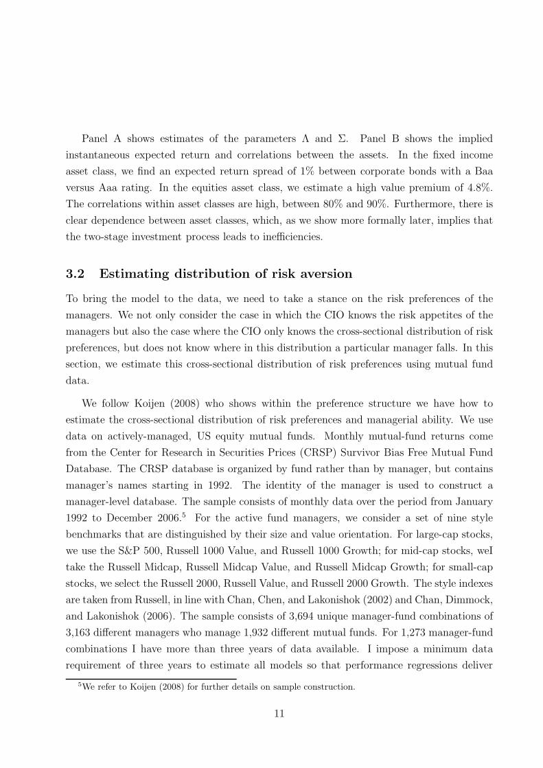
Panel A shows estimates of the parameters Λ and Σ. Panel B shows the implied

instantaneous expected return and correlations between the assets. In the fixed income

asset class, we find an expected return spread of 1% between corporate bonds with a Baa

versus Aaa rating. In the equities asset class, we estimate a high value premium of 4.8%.

The correlations within asset classes are high, between 80% and 90%. Furthermore, there is

clear dependence between asset classes, which, as we show more formally later, implies that

the two-stage investment process leads to inefficiencies.

3.2 Estimating distribution of risk aversion

To bring the model to the data, we need to take a stance on the risk preferences of the

managers. We not only consider the case in which the CIO knows the risk appetites of the

managers but also the case where the CIO only knows the cross-sectional distribution of risk

preferences, but does not know where in this distribution a particular manager falls. In this

section, we estimate this cross-sectional distribution of risk preferences using mutual fund

data.

We follow Koijen (2008) who shows within the preference structure we have how to

estimate the cross-sectional distribution of risk preferences and managerial ability. We use

data on actively-managed, US equity mutual funds. Monthly mutual-fund returns come

from the Center for Research in Securities Prices (CRSP) Survivor Bias Free Mutual Fund

Database. The CRSP database is organized by fund rather than by manager, but contains

manager’s names starting in 1992. The identity of the manager is used to construct a

manager-level database. The sample consists of monthly data over the period from January

1992 to December 2006.5 For the active fund managers, we consider a set of nine style

benchmarks that are distinguished by their size and value orientation. For large-cap stocks,

we use the S&P 500, Russell 1000 Value, and Russell 1000 Growth; for mid-cap stocks, weI

take the Russell Midcap, Russell Midcap Value, and Russell Midcap Growth; for small-cap

stocks, we select the Russell 2000, Russell Value, and Russell 2000 Growth. The style indexes

are taken from Russell, in line with Chan, Chen, and Lakonishok (2002) and Chan, Dimmock,

and Lakonishok (2006). The sample consists of 3,694 unique manager-fund combinations of

3,163 different managers who manage 1,932 different mutual funds. For 1,273 manager-fund

combinations I have more than three years of data available. I impose a minimum data

requirement of three years to estimate all models so that performance regressions deliver

5We refer to Koijen (2008) for further details on sample construction.

11

reasonably accurate estimates. For mutual funds, we consider a model in which the manager

can trade the style benchmark, an active portfolio, and a cash account. This resembles the

model we have, without the cash restriction and we consider the case where the managers

can trade multiple passive portfolios. In such a model and with the preferences we have,

the manager i’s alpha, beta and active risk are given by:

αi =λ2

Ai

γi

,

βi =λB

γiσB

+

(

1 −

1

γi

)

,

σεi =λAi

γi

.

see Koijen (2008) for further details. One can think of the active risk as the residual risk

in a standard performance regression. λB denotes the Sharpe ratio on the benchmark and

σB denotes the benchmark volatility. These two moments suffice to estimate the manager’s

risk aversion (γi) and ability (λAi). We use these moments to estimate the two attributes of

the manager and focus on the implied cross-sectional distribution of risk aversion across all

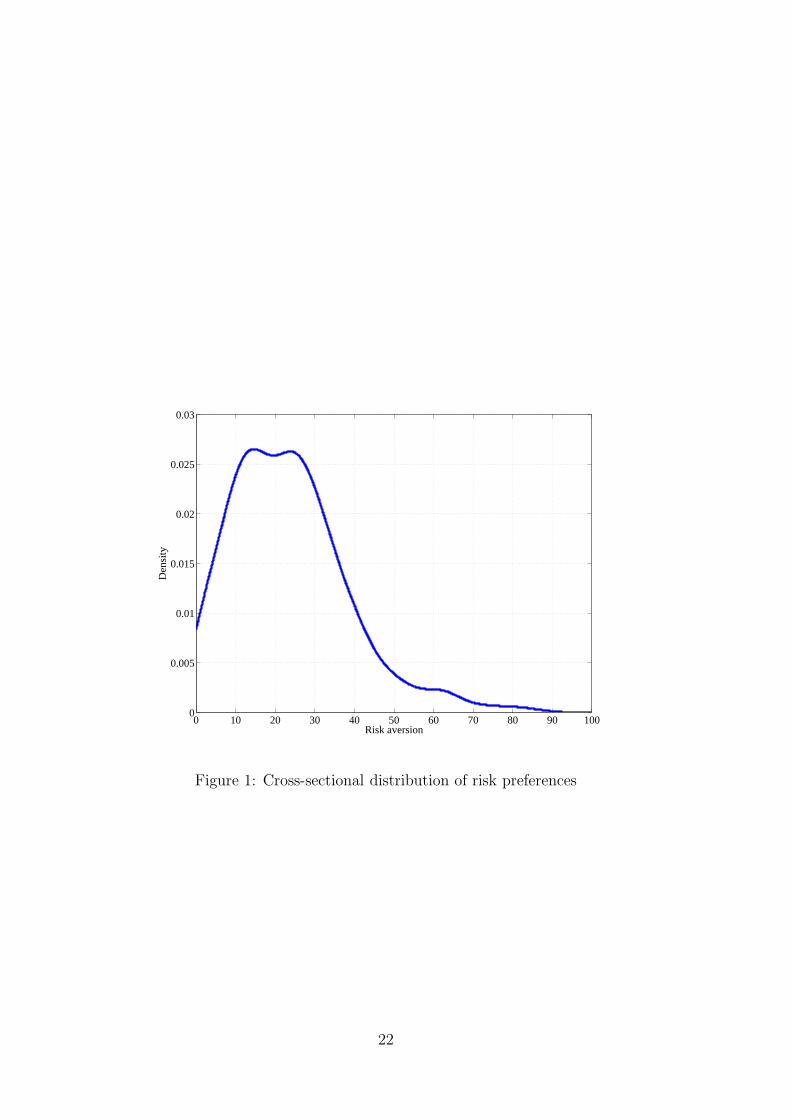
mutual fund managers. Figure 1 displays a non-parametric estimate of the cross-sectional

distribution of the coefficient of relative risk aversion. The average risk aversion across all

managers equals 25.92 and its standard deviation 51.19. The distribution is clearly right-

skewed. The high estimates for risk aversion resonate with the findings of Becker, Ferson,

Myers, and Schill (1999). The findings are also consistent with the ideas in the investment

management industry that manager are often rather conservative and act closely around

their benchmarks.

[Figure 1 about here.]

4 Main empirical results

To calibrate the model, we will assume that the return on the liabilities is like the return

on government bonds, that is, σL = σ1. Also, in computing the optimal portfolios with

cash benchmarks and the optimal benchmarks, we assume the managers are unskilled:

λA1 = λA2 = 0. We subsequently compute which levels of managerial ability would be

required to justify decentralized asset management.

12

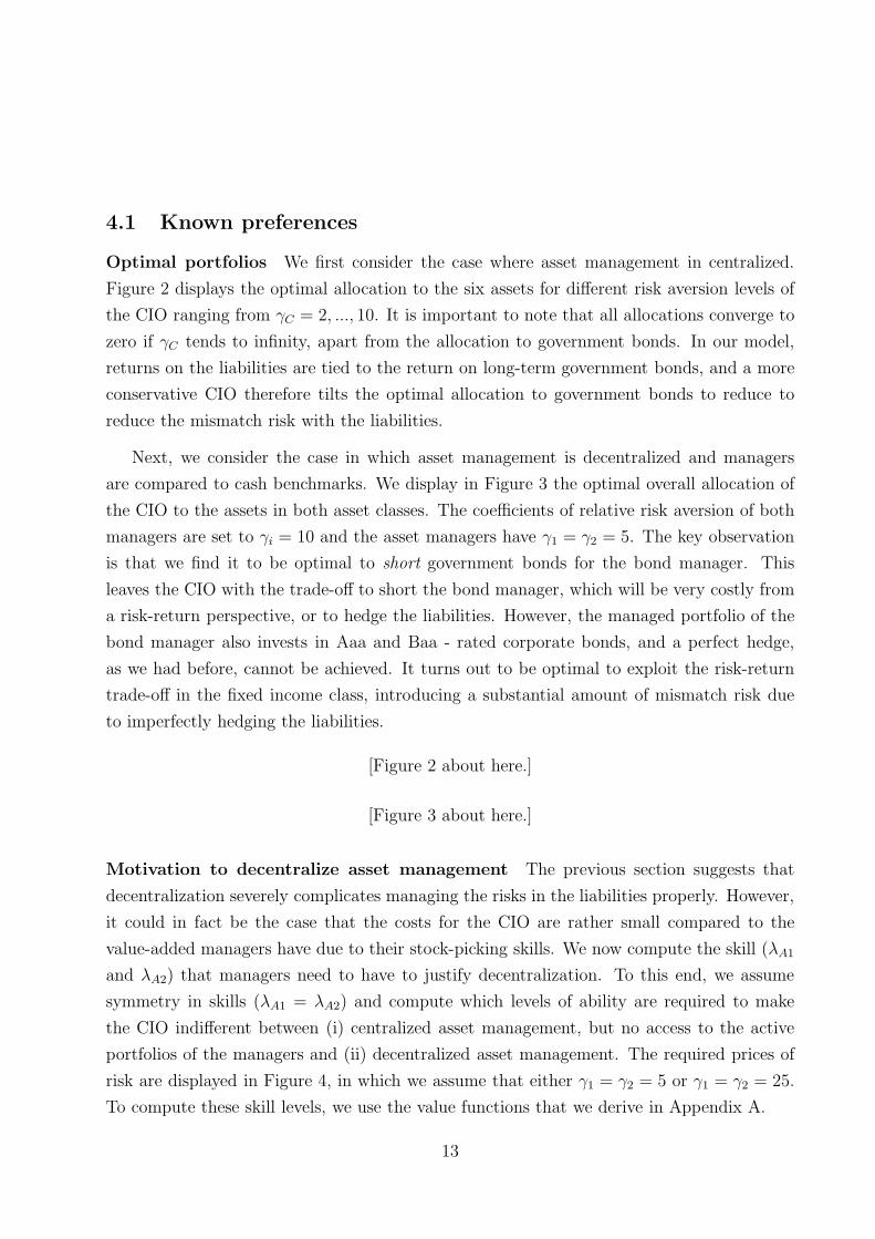
4.1 Known preferences

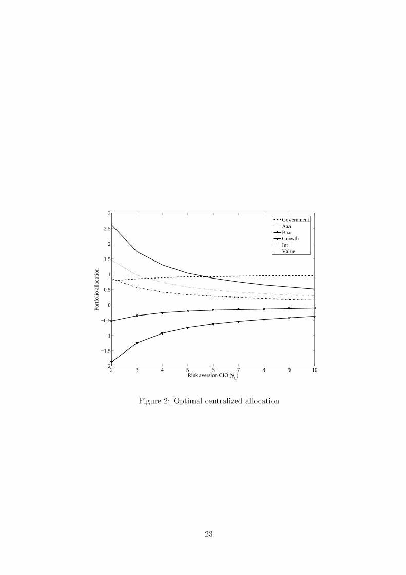
Optimal portfolios We first consider the case where asset management in centralized.

Figure 2 displays the optimal allocation to the six assets for different risk aversion levels of

the CIO ranging from γC = 2, ..., 10. It is important to note that all allocations converge to

zero if γC tends to infinity, apart from the allocation to government bonds. In our model,

returns on the liabilities are tied to the return on long-term government bonds, and a more

conservative CIO therefore tilts the optimal allocation to government bonds to reduce to

reduce the mismatch risk with the liabilities.

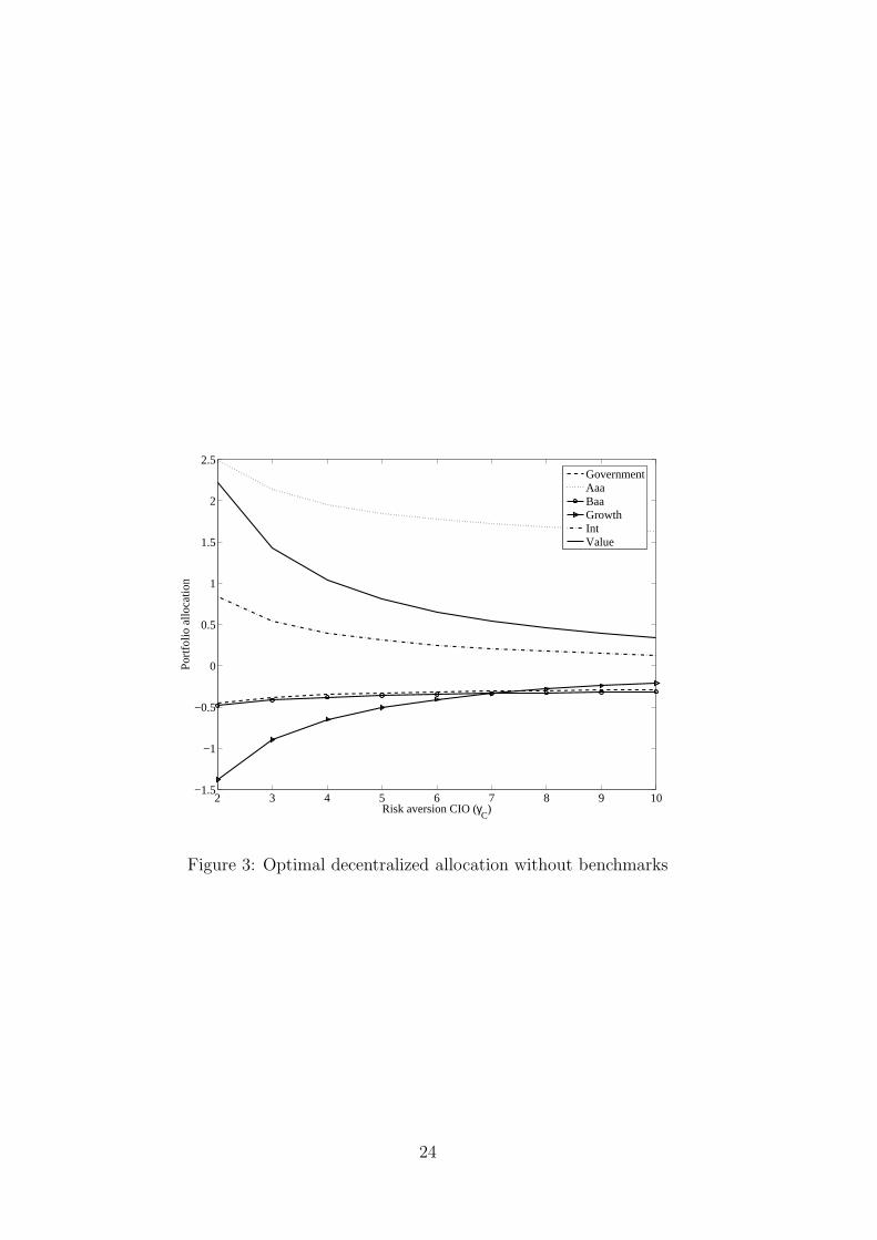
Next, we consider the case in which asset management is decentralized and managers

are compared to cash benchmarks. We display in Figure 3 the optimal overall allocation of

the CIO to the assets in both asset classes. The coefficients of relative risk aversion of both

managers are set to γi = 10 and the asset managers have γ1 = γ2 = 5. The key observation

is that we find it to be optimal to short government bonds for the bond manager. This

leaves the CIO with the trade-off to short the bond manager, which will be very costly from

a risk-return perspective, or to hedge the liabilities. However, the managed portfolio of the

bond manager also invests in Aaa and Baa - rated corporate bonds, and a perfect hedge,

as we had before, cannot be achieved. It turns out to be optimal to exploit the risk-return

trade-off in the fixed income class, introducing a substantial amount of mismatch risk due

to imperfectly hedging the liabilities.

[Figure 2 about here.]

[Figure 3 about here.]

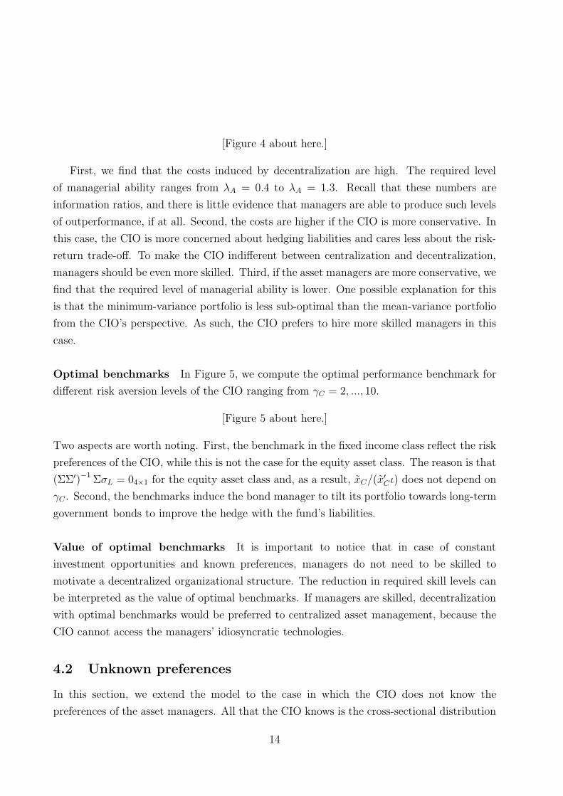
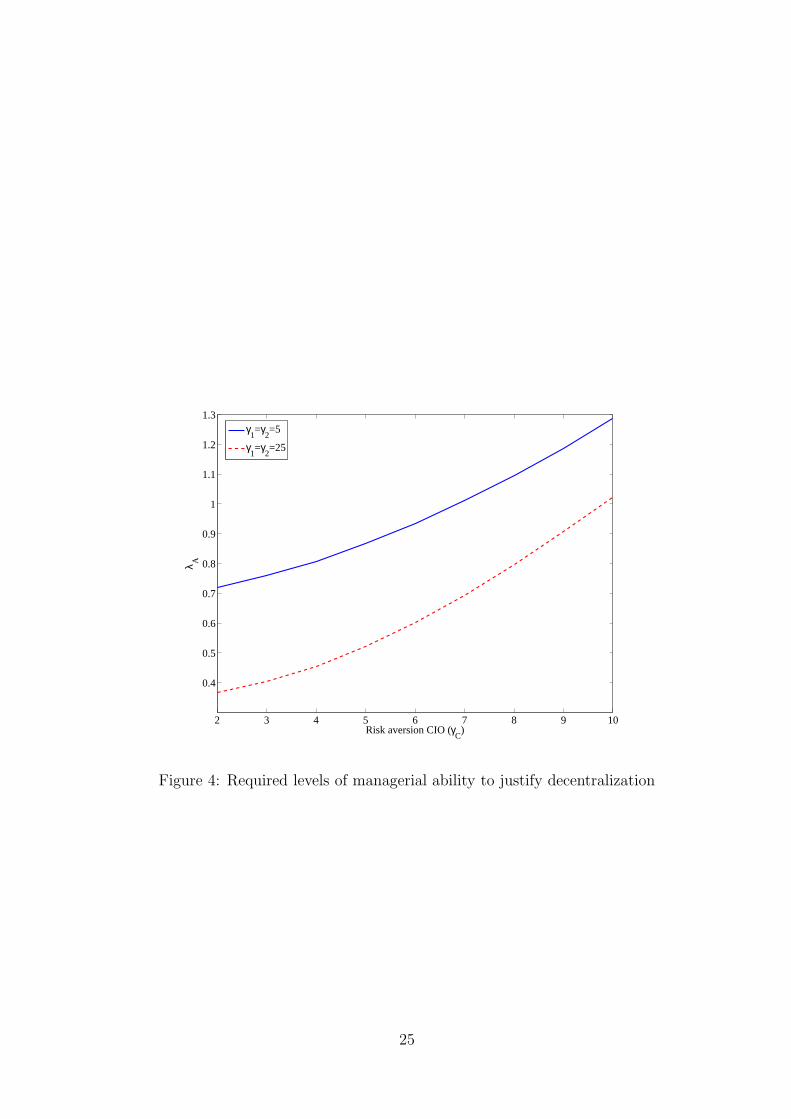
Motivation to decentralize asset management The previous section suggests that

decentralization severely complicates managing the risks in the liabilities properly. However,

it could in fact be the case that the costs for the CIO are rather small compared to the

value-added managers have due to their stock-picking skills. We now compute the skill (λA1

and λA2) that managers need to have to justify decentralization. To this end, we assume

symmetry in skills (λA1 = λA2) and compute which levels of ability are required to make

the CIO indifferent between (i) centralized asset management, but no access to the active

portfolios of the managers and (ii) decentralized asset management. The required prices of

risk are displayed in Figure 4, in which we assume that either γ1 = γ2 = 5 or γ1 = γ2 = 25.

To compute these skill levels, we use the value functions that we derive in Appendix A.

13

[Figure 4 about here.]

First, we find that the costs induced by decentralization are high. The required level

of managerial ability ranges from λA = 0.4 to λA = 1.3. Recall that these numbers are

information ratios, and there is little evidence that managers are able to produce such levels

of outperformance, if at all. Second, the costs are higher if the CIO is more conservative. In

this case, the CIO is more concerned about hedging liabilities and cares less about the risk-

return trade-off. To make the CIO indifferent between centralization and decentralization,

managers should be even more skilled. Third, if the asset managers are more conservative, we

find that the required level of managerial ability is lower. One possible explanation for this

is that the minimum-variance portfolio is less sub-optimal than the mean-variance portfolio

from the CIO’s perspective. As such, the CIO prefers to hire more skilled managers in this

case.

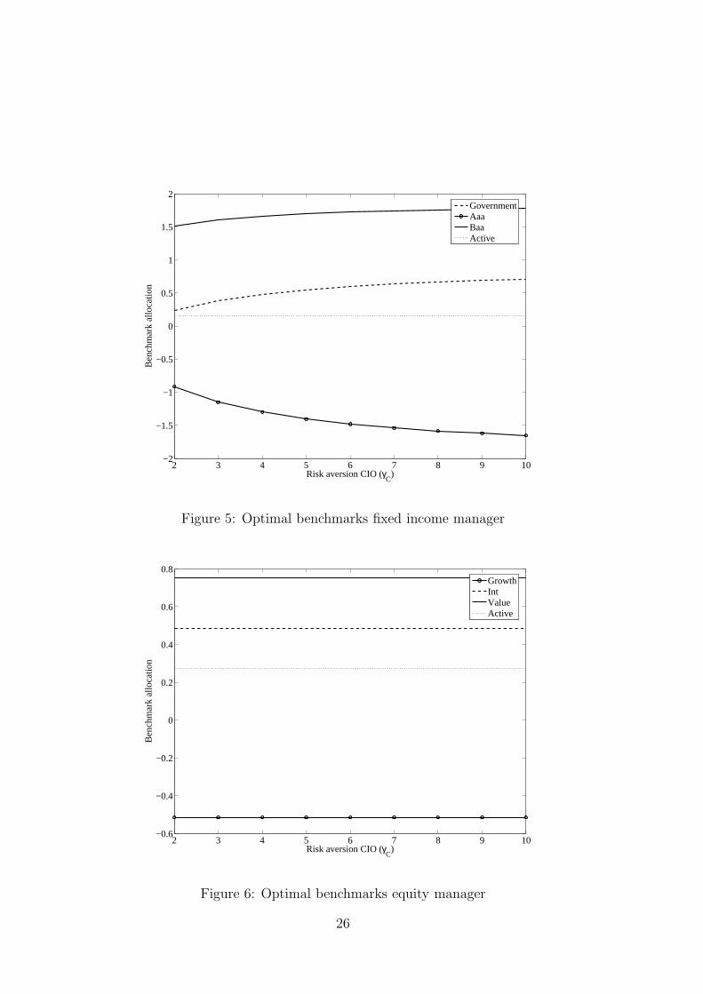
Optimal benchmarks In Figure 5, we compute the optimal performance benchmark for

different risk aversion levels of the CIO ranging from γC = 2, ..., 10.

[Figure 5 about here.]

Two aspects are worth noting. First, the benchmark in the fixed income class reflect the risk

preferences of the CIO, while this is not the case for the equity asset class. The reason is that

(ΣΣ′)−1 ΣσL = 04×1 for the equity asset class and, as a result, xC/(x′

Cι) does not depend on

γC . Second, the benchmarks induce the bond manager to tilt its portfolio towards long-term

government bonds to improve the hedge with the fund’s liabilities.

Value of optimal benchmarks It is important to notice that in case of constant

investment opportunities and known preferences, managers do not need to be skilled to

motivate a decentralized organizational structure. The reduction in required skill levels can

be interpreted as the value of optimal benchmarks. If managers are skilled, decentralization

with optimal benchmarks would be preferred to centralized asset management, because the

CIO cannot access the managers’ idiosyncratic technologies.

4.2 Unknown preferences

In this section, we extend the model to the case in which the CIO does not know the

preferences of the asset managers. All that the CIO knows is the cross-sectional distribution

14

of risk aversion levels that we estimate using mutual fund data. This cross-sectional

distribution is displayed in Figure 1. For simplicity, we assume that the risk aversion levels

of both managers are perfectly correlated.

Motivation to decentralize asset management In this case, we solve numerically for

the CIO’s allocation to both asset classes:

maxxC

E0

(

1

1 − γC

W 1−γC

T

)

. (1)

It is important to note that the expectation integrates out both uncertainty about future

asset returns and uncertainty about the risk appetites of asset managers.

We can simplify the problem by using the analytical value function derived earlier and

reported in Appendix A:

maxxC

E0

(

E

(

1

1 − γC

W 1−γC

T

∣

∣

∣

∣

γ1, γ2

))

= maxxC

1

1 − γC

W 1−γC

0 E0 (exp (a(xC , γ)TC)) . (2)

Along these lines, we are able to solve for the optimal strategic allocation to both asset

classes. With the optimal strategy of the CIO in hand, we compute the skill levels

(λA = λA1 = λA2) that ensure that the CIO is indifferent between centralized and

decentralized asset management.

5 Extensions

We briefly discuss two extensions of our model.

5.1 Portfolio constraints

Although institutional investors may be less restricted by short sales constraints, see for

instance Nagel (2005), it is plausible that shorting assets is costly for certain asset classes.

In this section, we briefly summarize how such constraints can be incorporated.

In case of constant investment opportunities, Tepla (2000) shows that the dynamic

problem can be solved using standard static techniques. I.e., solving for the optimal portfolio

of the asset managers entails solving a sequence of problems as before, but which a reduced

asset space. Once the portfolio constraints have been satisfied, we obtain a candidate solution

15

and finally optimize over all candidate solutions. If investment opportunities are time-

varying, we have to resort to numerical techniques, but these are particularly simple once we

impose the assumption of managerial myopia. After all, investors only incorporate current

investment opportunities, implying that we can determine the managers’ optimal portfolio

without solving a dynamic program.

The empirical application used throughout is not particularly suited for imposing

portfolio constraints, as the fixed income manager optimally shorts Aaa rated bonds to

finance investments in Baa rated bonds and similarly for the equity manager for growth and

value stocks. Consequently, we only obtain corner solutions.

5.2 Time-varying investment opportunities

In the model we have considered to far, risk premia are assumed to be constant. However, it

is well known that risk premia tend to move over time, see Cochrane (2007) and Binsbergen

and Koijen (2008) for stocks and Cochrane and Piazzesi (2005) for government bonds.

Binsbergen et al. (2008) incorporate return predictability in a model that does not feature

liabilities and managerial ability as we have. From a technical perspective, however, the

same derivations are suffice to extend our model to account for time-varying investment

opportunities. Binsbergen et al. (2008) show that in this case the costs of decentralized

asset management, and the value of optimally designed benchmarks, both increase. We refer

to their paper for a detailed analysis of a model with time-varying risk premia.

6 Conclusions

In this paper, we study the investment problem of a pension fund in which a centralized

decision maker, the Chief Investment Officer (CIO), for example, employs multiple asset

managers to implement investment strategies in separate asset classes. The CIO allocates

capital to the managers who, in turn, allocate these funds to the assets in their asset class. We

assume that managers have specific stock selection and market timing skills which allow them

to outperform passive benchmarks. However, the decentralized organizational structure also

induces several inefficiencies and misalignments of incentives including loss of diversification

and unobservable managerial appetite for risk. We show that if the CIO leaves the behavior

of the asset managers unaffected, which happens for instance if managers are remunerated

relative to a cash benchmark, the information ratio required to justify this organizational

16

structure ranges from 0.4 to 1.3. However, by using optimally designed benchmarks, we

can mitigate the inefficiencies induced by decentralization and can still realize the potential

benefits of managerial ability. Our framework suggests that the ability and performance of

the managers can influence the choice of organizational design of the fund, which in turn

influences the performance of the fund as a whole.

17

References

Admati, Anat R., and Paul Pfleiderer, 1997, Does it all add up? Benchmarks and thecompensation of active portfolio managers, Journal of Business 70, 323-350.

Barberis, Nicholas C., 2000, Investing for the long run when returns are predictable, Journal

of Finance 55, 225-264.

Basak, Suleyman, Alex Shapiro, and Lucie Tepla, 2006, Risk management withbenchmarking, Management Science 52, 542-557.

van Binsbergen, Jules H., and Michael W. Brandt, 2007, Optimal asset allocation in assetliability management, Working paper, Duke University.

van Binsbergen, Jules H., Michael W. Brandt, and Ralph S.J. Koijen, 2008, Optimaldecentralized investment management, Journal of Finance, August.

Brennan, Michael J., and Xia, Yihong, 2001, Stock price volatility and equity premium,Journal of Monetary Economics 47, 249-283.

Cochrane, John H., and Monika Piazzesi, 2005, Bond risk premia, American Economic

Review 95, 138-160.

Elton, Edwin J., and Martin J. Gruber, 2004, Optimum centralized portfolio constructionwith decentralized portfolio management, Journal of Financial and Quantitative

Analysis 39, 481-494.

Hoevenaars, Roy P.M.M., Roderick D.J. Molenaar, Peter C. Schotman, and Tom B.M.Steenkamp, Strategic Asset Allocation with Liabilities: Beyond Stocks and Bonds,Journal of Economic Dynamics and Control, forthcoming.

Koijen, Ralph S.J., 2008, The Cross-section of Managerial Ability and Risk Preferences,Working paper, University of Chicago.

Ou-Yang, Hui, 2003, Optimal contracts in a continuous-time delegated portfolio managementproblem, Review of Financial Studies 16, 173-208.

Sharpe, William F., 1981, Decentralized investment management, Journal of Finance 36,217-234.

Stracca, Livio, 2006, Delegated portfolio management: A survey of the theoretical literature,Journal of Economic Surveys 20, 823-848.

Tepla, Lucie, 2000, Optimal portfolio policies with borrowing and shortsale constraints,Journal of Economic Dynamics & Control 24, 1623-1639.

Vayanos, Dimitri, 2003, The decentralization of information processing in the presence ofinteractions, Review of Economic Studies 70, 667-695.

18

A Value functions

In this appendix, we summarize the value functions of the CIO of the different problems.

A.1 Known preferences

Centralized problem The value function takes the form:

J (F, τC) =1

1 − γC

F 1−γC exp (a(x)τC) ,

with τC = TC − t and x the (implied) portfolio choice of the CIO, which equals:

x =1

γC

(ΣCΣ′

C)−1

ΣCΛC +

(

1 −

1

γC

)

(ΣCΣ′

C)−1

ΣCσL,

in this case. The function a(x) reads:

a(x) = (1 − γC) (r + x′ΣCΛC − µL + σ′

LσL − x′ΣCσL)

−

1

2γC (1 − γC) (x′ΣC − σ′

L) (Σ′

Cx − σL) ,

which can be derived using standard dynamic programming techniques.

Decentralized with cash benchmarks The value function in this case takes the sameform, but the function a(x) changes because the CIO can now access the idiosyncratictechnologies via the managers:

a(x) = (1 − γC) (r + x′ΣΛ − µL + σ′

LσL − x′ΣσL)

−

1

2γC (1 − γC) (x′Σ − σ′

L) (Σ′x − σL) ,

and the optimal (implied) portfolio reads:

x =

[

xCashC(1) xCash

1

xCashC(2) xCash

2

]

.

Decentralized with optimal benchmarks In case of optimal benchmarks, the CIO canachieve first-best, but with access to the idiosyncratic technologies. As such, a(x) is of theform:

a(x) = (1 − γC) (r + x′ΣΛ − µL + σ′

LσL − x′ΣσL)

−

1

2γC (1 − γC) (x′Σ − σ′

L) (Σ′x − σL) ,

19

with a portfolio:

x =1

γC

(ΣΣ′)−1

ΣΛ +

(

1 −

1

γC

)

(ΣΣ′)−1

ΣσL.

A.2 Unknown preferences

20

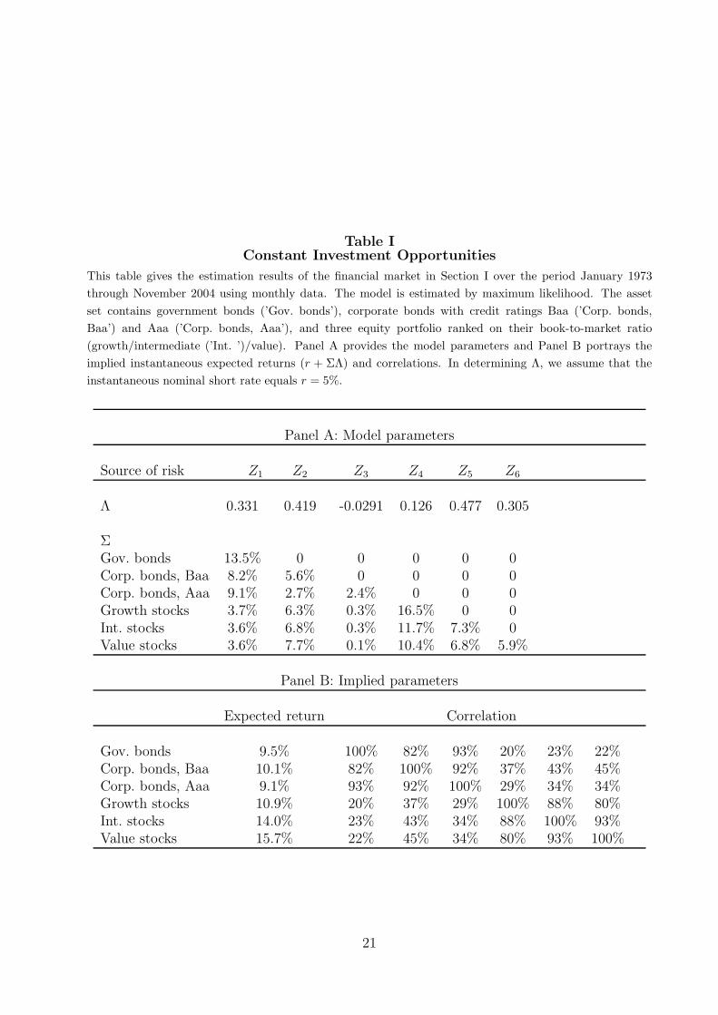
Table IConstant Investment Opportunities

This table gives the estimation results of the financial market in Section I over the period January 1973

through November 2004 using monthly data. The model is estimated by maximum likelihood. The asset

set contains government bonds (’Gov. bonds’), corporate bonds with credit ratings Baa (’Corp. bonds,

Baa’) and Aaa (’Corp. bonds, Aaa’), and three equity portfolio ranked on their book-to-market ratio

(growth/intermediate (’Int. ’)/value). Panel A provides the model parameters and Panel B portrays the

implied instantaneous expected returns (r + ΣΛ) and correlations. In determining Λ, we assume that the

instantaneous nominal short rate equals r = 5%.

Panel A: Model parameters

Source of risk Z1 Z2 Z3 Z4 Z5 Z6

Λ 0.331 0.419 -0.0291 0.126 0.477 0.305

ΣGov. bonds 13.5% 0 0 0 0 0Corp. bonds, Baa 8.2% 5.6% 0 0 0 0Corp. bonds, Aaa 9.1% 2.7% 2.4% 0 0 0Growth stocks 3.7% 6.3% 0.3% 16.5% 0 0Int. stocks 3.6% 6.8% 0.3% 11.7% 7.3% 0Value stocks 3.6% 7.7% 0.1% 10.4% 6.8% 5.9%

Panel B: Implied parameters

Expected return Correlation

Gov. bonds 9.5% 100% 82% 93% 20% 23% 22%Corp. bonds, Baa 10.1% 82% 100% 92% 37% 43% 45%Corp. bonds, Aaa 9.1% 93% 92% 100% 29% 34% 34%Growth stocks 10.9% 20% 37% 29% 100% 88% 80%Int. stocks 14.0% 23% 43% 34% 88% 100% 93%Value stocks 15.7% 22% 45% 34% 80% 93% 100%

21

0 10 20 30 40 50 60 70 80 90 1000

0.005

0.01

0.015

0.02

0.025

0.03

Risk aversion

Den

sity

Figure 1: Cross-sectional distribution of risk preferences

22

2 3 4 5 6 7 8 9 10−2

−1.5

−1

−0.5

0

0.5

1

1.5

2

2.5

3

Risk aversion CIO (γC)

Por

tfolio

allo

catio

n

GovernmentAaaBaaGrowthIntValue

Figure 2: Optimal centralized allocation

23

2 3 4 5 6 7 8 9 10−1.5

−1

−0.5

0

0.5

1

1.5

2

2.5

Risk aversion CIO (γC)

Por

tfolio

allo

catio

n

GovernmentAaaBaaGrowthIntValue

Figure 3: Optimal decentralized allocation without benchmarks

24

2 3 4 5 6 7 8 9 10

0.4

0.5

0.6

0.7

0.8

0.9

1

1.1

1.2

1.3

Risk aversion CIO (γC)

λ A

γ1=γ

2=5

γ1=γ

2=25

Figure 4: Required levels of managerial ability to justify decentralization

25

2 3 4 5 6 7 8 9 10−2

−1.5

−1

−0.5

0

0.5

1

1.5

2

Risk aversion CIO (γC)

Ben

chm

ark

allo

catio

n

GovernmentAaaBaaActive

Figure 5: Optimal benchmarks fixed income manager

2 3 4 5 6 7 8 9 10−0.6

−0.4

−0.2

0

0.2

0.4

0.6

0.8

Risk aversion CIO (γC)

Ben

chm

ark

allo

catio

n

GrowthIntValueActive

Figure 6: Optimal benchmarks equity manager

26