Embed Size (px)
Citation preview

PEAS: Package for Elementary Analysis of SNP data
Designed by Shuhua Xu and Li Jin
Code by Shuhua Xu
with contributions from Sanchit Gupta
January 8, 2010
Contact information Shuhua Xu Ph.D., CAS-MPG Partner Institute of Computational Biology, SIBS, CAS 320 YueYang Road, Shanghai 200031, China Phone: 86-21-54920479 Fax: 86-21-54920451 E-mail: [email protected] E-mail: [email protected] Website: http://www.picb.ac.cn/~xushua

Contents 1 Introduction ................................................................................................................................ 3 2 Overview ..................................................................................................................................... 4 3 Download and installation ...................................................................................................... 5
3.1 System requirements ......................................................................................................... 5 3.2 PEAS Component Programs ............................................................................................ 6 3.3 GUI for PEAS .................................................................................................................... 7
4 Format for the data file ............................................................................................................ 8 4.1 Standard format for the genotype data file ..................................................................... 8 4.2 Alternative format for the genotype data file ................................................................. 9
4.2.1 SNPs in rows and individuals in columns ............................................................ 9 4.2.1.1 Genotype coded by single character ........................................................ 10 4.2.1.2 Genotype coded by two characters .......................................................... 11
4.2.2 Individuals in rows and SNPs in columns .......................................................... 12 4.2.2.1 Genotype coded by single character ........................................................ 13 4.2.2.2 Genotype coded by two characters .......................................................... 13
5 Functions in Component Programs ................................................................................... 14 5.1 Basic data format conversion tools. ............................................................................... 14 5.2 Data Splitting ................................................................................................................... 17 5.3 Data Filtering ................................................................................................................... 18 5.4 Consensus Markers ......................................................................................................... 20 5.5 Data integration ............................................................................................................... 20 5.6 Basic Statistics ................................................................................................................. 21 5.7 Data Sampling ................................................................................................................. 22 5.8 Individual Distance ......................................................................................................... 24 5.9 Population Distance ........................................................................................................ 25 5.10 LD calculator ................................................................................................................. 26 5.11 Haplotype sharing analysis. .......................................................................................... 27 5.12 Other Software Input .................................................................................................... 28
6 Functions in GUI ..................................................................................................................... 29 6.1 Basic data format conversion tools. ............................................................................... 29 6.1.2 Two format conversion tools to transpose data between columns and rows. .......... 30 6.1.3 Genotype coding transformation ................................................................................ 30 6.2 Data split .......................................................................................................................... 31 6.2.1 Split data by samples ................................................................................................... 31 6.2.2 Split data by markers................................................................................................... 39
6.3 Data filtering .......................................................................................................................... 40 6.4 Search shared loci .............................................................................................................. 41 6.5 Data combination ................................................................................................................. 42 6.6 Basic statistics ..................................................................................................................... 43
6.6.1 Allele count.................................................................................................................... 43 6.6.2 Allele frequency ............................................................................................................ 44 6.6.3 Genotype count ............................................................................................................. 45
1

6.6.4 Genotype frequency ..................................................................................................... 46 6.6.5 Hardy-Weinberg equilibrium (p-value threshold, 0.05) ........................................... 46
6.7 Population genetic distances ........................................................................................... 47 6.7.1 Estimates of FST ............................................................................................................ 47 6.7.2 F*ST Distance ................................................................................................................ 48 6.7.3 Nei’s Standard Distance ............................................................................................... 49 6.7.4 Cavalli-Sforza’s dC........................................................................................................ 50 6.7.5 Nei’s DA ......................................................................................................................... 50 6.7.6 Output distance matrix for MEGA and PHYLIP analysis ....................................... 51 6.7.7 Bootstrapping for distance calculation ....................................................................... 51
6.8 Individual genetic distances ............................................................................................. 51 6.8.1 Allele sharing distance ................................................................................................. 51
6.9 Input files for other programs .......................................................................................... 53 6.9.1 Format input files for PHASE ..................................................................................... 53 6.9.2 Format input files for fastPHASE .............................................................................. 53 6.9.3 Format input files for STRUCTURE ......................................................................... 53 6.9.4 Format input files for Arlequin ................................................................................... 53 6.9.5 Format input files for Haploview ................................................................................ 54 6.9.6 Format input files for LDhat ....................................................................................... 54
6.10 Linkage Disequilibrium .................................................................................................... 54 6.10.1 Measures of Linkage Disequilibrium ....................................................................... 54
7 How to cite this program ...................................................................................................... 55 8 References ................................................................................................................................ 56
2

1 Introduction Owing to the advent of high-throughput biological and chemical assays, a wealth of
genomic data has been created, of which single nucleotide polymorphism (SNP) data
accumulate especially fast. With the release of the Phase III HapMap (The
International HapMap Consortium, 2003; 2005; http://www.hapmap.org) data, a
resource consisting of over 1.6 million SNPs genotyped in more than 1000
individuals from 11 geographically diverse populations is publicly available. Many
similar private or international projects focus on a special of group of genes such as
Environmental Genome Project (EGP; http://www.niehs.nih.gov/envgenom) or on
regional populations such as PanAsian SNP Project (PASNP;
http://pasnpi.biotec.or.th/) generated additional SNP data resources. The modern
human genetic studies have been dramatically influenced by the development and
release of these data, our insight and knowledge about human genome has been
greatly improved due to the analysis of those SNP data.
Many software tools have been developed to extract abundant information from
ssuch data. Most of software tools available focus on a certain purpose and perform
well on one special aspect. PHASE (Stephens, Smith et al. 2001) is one of the best
software tools available for inferring haplotypes from population genotype data; the
fastPHASE (Scheet and Stephens 2006) program that developed subsequently
performed well in inferring haplotypes in large SNP surveys; Haploview (Barrett, Fry
et al. 2005) is widely used software in LD & Haplotype block analysis and tag SNP
selection; LDhat (McVean, Myers et al. 2004) is the software tool developed for
fine-scale recombination analysis and it performs well in high density SNP data. In
addition, a few software tools, which although were developed earlier and not limited
in SNP data, are still useful in population genetic analysis of SNP data, for instance,
Arlequin (Schneider, Roessli et al. 2000) provides a large set of tools with basic
methods in population genetics; STRUCTURE (Pritchard, Stephens et al. 2000;
Falush, Stephens et al. 2003) is one of the best software tools available for inferring
population structure using genotype data. However, all most all software tools
3
available have been developed for some specific purpose and have private format of
input files, whereas both the formatting jobs of input file and manipulation of output
files often take people much time, especially for those biologists who do not write
program themselves and when the data set is very large. Furthermore, there are still
many gaps of analysis for the current available software, such as calculating
individual allele sharing distance, population genetic distances, do bootstrapping,
calculating LD statistics for large-scale SNP data set and so on. For some basic data
manipulations, either the software available currently do not provide or the software
do not work very well for large data sets.
Here we developed a software package named PEAS to provide the average user
with many basic analysis tools and facilitate people who are involving in analysis of
large SNP data set.
2 Overview
All the programs in PEAS are developed to handle very large amount of SNP data
with high efficiency. We adopt dynamic memory management, so there is actually no
limit of the program for the size of data set, the only limit is the memory of the
computer. All the operations of PEAS programs are file(s) to file(s), although PEAS
allow the user display results in the GUI which will take huge memory to display on
the screen, especially for very large data set. We recommend the user chose not to
display data and let program perform background process. In that case, we also
provide single separate executables for each PEAS function, so alternatively the user
can find all the PEAS component programs separate single executables in the PEAS
directory, we will show the details in the following sections.
PEAS is versatile in manipulating data. We provide many tools in PEAS for data
formatting, which will facilitate the user manipulate data by easy stages before they
proceed further analysis. Secondly, we provide tools for some basic manipulations of
SNP data. Thirdly, to fill up the gaps of currently available software tools, a few tools
focus on population genetic analysis and phylogenetic analysis were implemented.
4
Finally, a graphical user interface is designed to facilitate the user to rapidly select
different PEAS tools and manipulate their data. A screenshot of the GUI of PEAS is
shown in Figure 1.
3 Download and installation PEAS for windows are freely available for academic user from the web
page http://www.picb.ac.cn/~xushua/index.files/Software.htm.
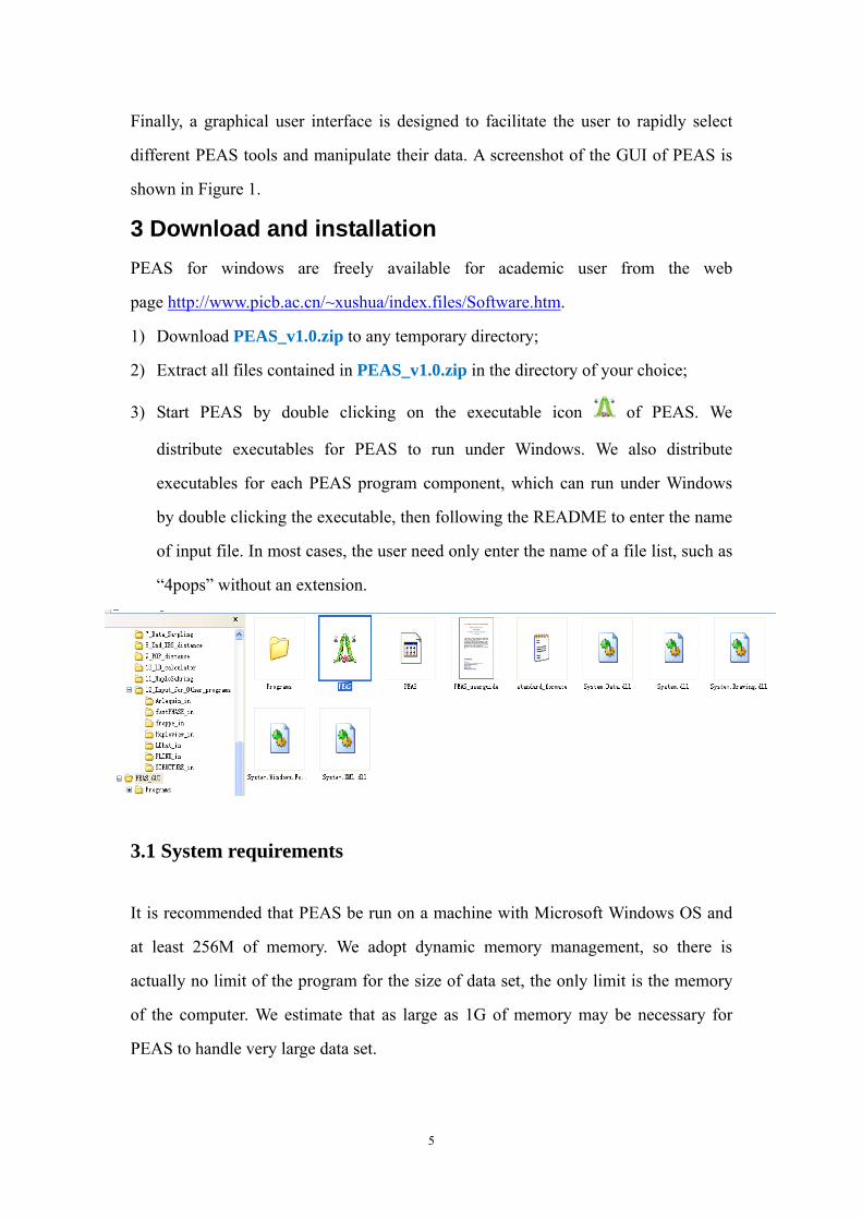
1) Download PEAS_v1.0.zip to any temporary directory;
2) Extract all files contained in PEAS_v1.0.zip in the directory of your choice;
3) Start PEAS by double clicking on the executable icon of PEAS. We
distribute executables for PEAS to run under Windows. We also distribute
executables for each PEAS program component, which can run under Windows
by double clicking the executable, then following the README to enter the name
of input file. In most cases, the user need only enter the name of a file list, such as
“4pops” without an extension.
3.1 System requirements
It is recommended that PEAS be run on a machine with Microsoft Windows OS and
at least 256M of memory. We adopt dynamic memory management, so there is
actually no limit of the program for the size of data set, the only limit is the memory
of the computer. We estimate that as large as 1G of memory may be necessary for
PEAS to handle very large data set.
5

3.2 PEAS Component Programs
As we described above, we provide individual component programs for each PEAS function. The user can find all the PEAS component programs separate executables in the PEAS directory, the following snapshot shows the overall structure of the PEAS component programs. Please note that currently not all functions available in GUI, but alternatively the user can perform all the analyses using PEAS component programs.
6

3.3 GUI for PEAS
We provide a GUI for PEAS user only to facilitate the user to manage the programs and files of both input and output. All the operations of PEAS programs are file to file, so there is no data loading to GUI to read, just let the program to locate the input files and save the output files in a user defined location.
Fig. 1. Screenshot of the user graphical interface of PEAS, showing the main page of
PEAS and the bottom plot displays the tools list.
The user can find all the analysis tools in the “Tools” menu, as shown in the following figure. The menu is the windows style that many MS windows OS users are familiar with.
Fig. 2. Screenshot of the user graphical interface of PEAS, showing the tools list.
7
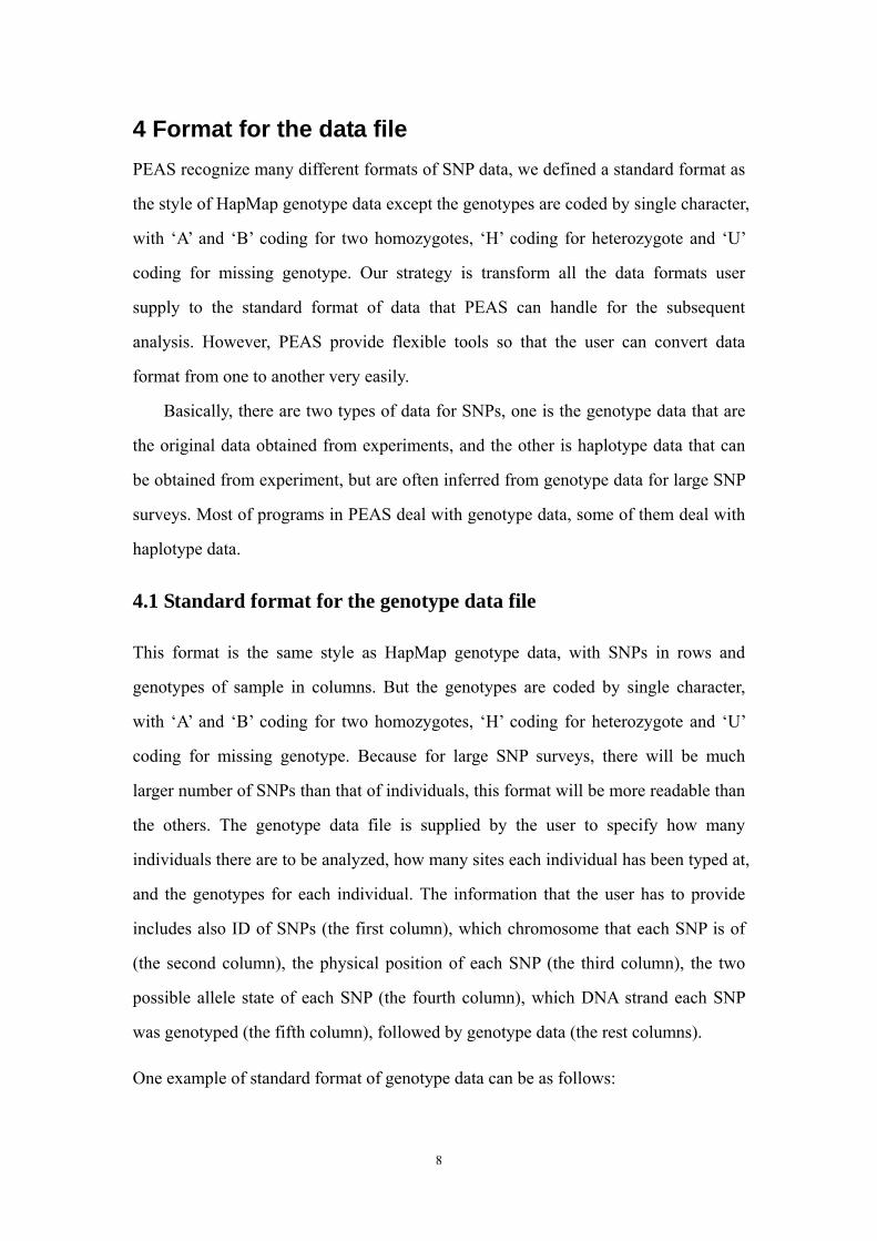
4 Format for the data file PEAS recognize many different formats of SNP data, we defined a standard format as
the style of HapMap genotype data except the genotypes are coded by single character,
with ‘A’ and ‘B’ coding for two homozygotes, ‘H’ coding for heterozygote and ‘U’
coding for missing genotype. Our strategy is transform all the data formats user
supply to the standard format of data that PEAS can handle for the subsequent
analysis. However, PEAS provide flexible tools so that the user can convert data
format from one to another very easily.
Basically, there are two types of data for SNPs, one is the genotype data that are
the original data obtained from experiments, and the other is haplotype data that can
be obtained from experiment, but are often inferred from genotype data for large SNP
surveys. Most of programs in PEAS deal with genotype data, some of them deal with
haplotype data.
4.1 Standard format for the genotype data file
This format is the same style as HapMap genotype data, with SNPs in rows and
genotypes of sample in columns. But the genotypes are coded by single character,
with ‘A’ and ‘B’ coding for two homozygotes, ‘H’ coding for heterozygote and ‘U’
coding for missing genotype. Because for large SNP surveys, there will be much
larger number of SNPs than that of individuals, this format will be more readable than
the others. The genotype data file is supplied by the user to specify how many
individuals there are to be analyzed, how many sites each individual has been typed at,
and the genotypes for each individual. The information that the user has to provide
includes also ID of SNPs (the first column), which chromosome that each SNP is of
(the second column), the physical position of each SNP (the third column), the two
possible allele state of each SNP (the fourth column), which DNA strand each SNP
was genotyped (the fifth column), followed by genotype data (the rest columns).
One example of standard format of genotype data can be as follows:
8

SNPID Chrom Position AlleleState Strand SampleID1 SampleID2 SampleID3
rs11089130 chr22 14431347 C/G + B A H
rs915675 chr22 14433659 A/C + H B A
rs915677 chr22 14433758 A/G + B B B
rs9604721 chr22 14434713 C/T + A H A
rs12159982 chr22 14434960 C/T + A A H
rs4389403 chr22 14435070 A/G + H B A
rs12628452 chr22 14435171 A/G + A B U
rs7291810 chr22 14435207 C/T + A H A
rs5746356 chr22 14439734 C/T + A H H
rs759235 chr22 15647006 A/G – H A B
rs5748656 chr22 15668200 C/T + B H B
rs5748657 chr22 15668220 C/T + H A A
rs2286985 chr22 15668377 G/T – A H B
rs2072467 chr22 15668988 A/G – H ? A
rs2072466 chr22 15669118 A/G – A H H
rs5746901 chr22 15670010 G/T + B H H
Note 1: Genotypes are coded in as A, B, H, here A and B indicate two homozygotes, and H
indicate heterozygote. Missing alleles can either be coded as U or as ?.
Note 2: All the formats including both the standard format and the following alternative formats
are restricted to those sites that have at most 2 alleles segregating. For those sites there are more
than 2 alleles present, we select the two most frequent alleles, and treat all the other alleles as
missing data.
Note 3: There could be extra columns between the strand column (the fifth column) and the
genotype columns (the sixth column and the following columns). The used can specify the number
of extra columns in the input files.
4.2 Alternative format for the genotype data file
Besides of the standard format, PEAS recognize 7 alternative formats.
4.2.1 SNPs in rows and individuals in columns
The layouts of the following three formats are the same as the standard format, i.e.
9

rows store the information of SNPs and columns store the information of individuals.
The only difference is the coding of genotype. The user provides SNP ID in the first
column, chromosome number in the second column, the physical position of each
SNP in the third column, the allele state of each SNP in the fourth column, DNA
strand of each SNP in the fifth column and followed by genotype data (the rest
columns).
4.2.1.1 Genotype coded by single character
The format is the same as the default except genotypes are coded in as 1, 2, 3, here 1
and 2 indicate two homozygotes, and 3 indicate heterozygote. Missing alleles can
either be coded as 0 or as ?.
SNPID Chrom Position AlleleState Strand SampleID1 SampleID2 SampleID3
rs11089130 chr22 14431347 C/G + 2 1 3
rs915675 chr22 14433659 A/C + 3 2 1
rs915677 chr22 14433758 A/G + 2 2 2
rs9604721 chr22 14434713 C/T + 1 3 1
rs12159982 chr22 14434960 C/T + 1 1 3
rs4389403 chr22 14435070 A/G + 3 2 1
rs12628452 chr22 14435171 A/G + 1 2 0
rs7291810 chr22 14435207 C/T + 1 3 1
rs5746356 chr22 14439734 C/T + 1 3 3
rs759235 chr22 15647006 A/G – 3 1 2
rs5748656 chr22 15668200 C/T + 2 3 2
rs5748657 chr22 15668220 C/T + 3 1 1
rs2286985 chr22 15668377 G/T – 1 3 2
rs2072467 chr22 15668988 A/G – 3 ? 1
rs2072466 chr22 15669118 A/G – 1 3 3
rs5746901 chr22 15670010 G/T + 2 3 3
10

4.2.1.2 Genotype coded by two characters
Each genotype is indicated by two characters, and the genotypes of each SNP are
listed on a single line, locus by locus. Genotypes can be coded in as standard DNA
letters, A, C, G, T; missing alleles can either be coded as N or as ?.
SNPID Chrom Position AlleleState Strand SampleID1 SampleID2 SampleID3
rs11089130 chr22 14431347 C/G + GG CC CG
rs915675 chr22 14433659 A/C + AC CC AA
rs915677 chr22 14433758 A/G + GG GG GG
rs9604721 chr22 14434713 C/T + CC CT CC
rs12159982 chr22 14434960 C/T + CC CC CT
rs4389403 chr22 14435070 A/G + AG GG AA
rs12628452 chr22 14435171 A/G + AA GG NN
rs7291810 chr22 14435207 C/T + CC CT CC
rs5746356 chr22 14439734 C/T + CC CT CT
rs759235 chr22 15647006 A/G – AG AA GG
rs5748656 chr22 15668200 C/T + TT CT TT
rs5748657 chr22 15668220 C/T + CT CC CC
rs2286985 chr22 15668377 G/T – GG GT TT
rs2072467 chr22 15668988 A/G – AG ?? AA
rs2072466 chr22 15669118 A/G – AA AG AG
rs5746901 chr22 15670010 G/T + TT GT GT
Genotypes can also be coded in as 11, 22, 12, here 11 and 22 indicate two
homozygotes, and 12 indicate heterozygote. Missing alleles can either be coded as 0
or as ?.
11

SNPID Chrom Position AlleleState Strand SampleID1 SampleID2 SampleID3
rs11089130 chr22 14431347 C/G + 22 11 12
rs915675 chr22 14433659 A/C + 12 22 11
rs915677 chr22 14433758 A/G + 22 22 22
rs9604721 chr22 14434713 C/T + 11 12 11
rs12159982 chr22 14434960 C/T + 11 11 12
rs4389403 chr22 14435070 A/G + 12 22 11
rs12628452 chr22 14435171 A/G + 11 22 00
rs7291810 chr22 14435207 C/T + 11 12 11
rs5746356 chr22 14439734 C/T + 11 12 12
rs759235 chr22 15647006 A/G – 12 11 22
rs5748656 chr22 15668200 C/T + 22 12 22
rs5748657 chr22 15668220 C/T + 12 11 11
rs2286985 chr22 15668377 G/T – 11 12 22
rs2072467 chr22 15668988 A/G – 12 ?? 11
rs2072466 chr22 15669118 A/G – 11 12 12
rs5746901 chr22 15670010 G/T + 22 12 12
4.2.2 Individuals in rows and SNPs in columns
In some studies, people prefer to provide another format of genotype data. This
format can be taken as a transpose of the layout of the default format, with SNPs in
columns and individuals in rows. The genotype data file is supplied by the user to
specify how many individuals there are to be analyzed, how many sites each
individual has been typed at, and the genotypes for each individual. The information
that the user has to provide includes also ID of SNPs (the first row), which
chromosome that each SNP is of (the second row), the physical position of each SNP
(the third row), the two possible allele state of each SNP (the fourth row), which DNA
strand each SNP was genotyped (the fifth row), followed by genotype data (the rest
rows).
12

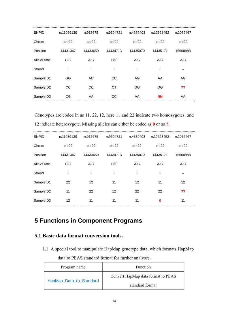
4.2.2.1 Genotype coded by single character
Genotypes are coded in as A, B, H, here A and B indicate two homozygotes, and H
indicate heterozygote. Missing alleles can either be coded as U or as ?.
SNPID rs11089130 rs915675 rs9604721 rs4389403 rs12628452 rs2072467
Chrom chr22 chr22 chr22 chr22 chr22 chr22
Position 14431347 14433659 14434713 14435070 14435171 15668988
AlleleState C/G A/C C/T A/G A/G A/G
Strand + + + + + –
SampleID1 B H A H A H
SampleID2 A B H B B ?
SampleID3 H A A A U A
Genotypes are coded in as 1, 2, 3, here 1 and 2 indicate two homozygotes, and 3
indicate heterozygote. Missing alleles can either be coded as 0 or as ?.
SNPID rs11089130 rs915675 rs9604721 rs4389403 rs12628452 rs2072467
Chrom chr22 chr22 chr22 chr22 chr22 chr22
Position 14431347 14433659 14434713 14435070 14435171 15668988
AlleleState C/G A/C C/T A/G A/G A/G
Strand + + + + + –
SampleID1 2 3 1 3 1 3
SampleID2 1 2 3 2 2 ?
SampleID3 3 1 1 1 0 1
4.2.2.2 Genotype coded by two characters
Each genotype is indicated by two characters, and the genotypes of each SNP are
listed on a single line, locus by locus. Genotypes are coded in as standard DNA letters,
A, C, G, T; missing alleles can either be coded as N or as ?.
13
SNPID rs11089130 rs915675 rs9604721 rs4389403 rs12628452 rs2072467
Chrom chr22 chr22 chr22 chr22 chr22 chr22
Position 14431347 14433659 14434713 14435070 14435171 15668988
AlleleState C/G A/C C/T A/G A/G A/G
Strand + + + + + –
SampleID1 GG AC CC AG AA AG
SampleID2 CC CC CT GG GG ??
SampleID3 CG AA CC AA NN AA
Genotypes are coded in as 11, 22, 12, here 11 and 22 indicate two homozygotes, and
12 indicate heterozygote. Missing alleles can either be coded as 0 or as ?.
SNPID rs11089130 rs915675 rs9604721 rs4389403 rs12628452 rs2072467
Chrom chr22 chr22 chr22 chr22 chr22 chr22
Position 14431347 14433659 14434713 14435070 14435171 15668988
AlleleState C/G A/C C/T A/G A/G A/G
Strand + + + + + –
SampleID1 22 12 11 12 11 12
SampleID2 11 22 12 22 22 ??
SampleID3 12 11 11 11 0 11
5 Functions in Component Programs
5.1 Basic data format conversion tools.
1.1 A special tool to manipulate HapMap genotype data, which formats HapMap
data to PEAS standard format for further analyses.
Program name Function
HapMap_Data_to_Standard Convert HapMap data format to PEAS
standard format
14

Procedure to run the program: [1] Double click the executable file;
[2] Enter the infile name:(e.g. genotypes_chr22_CHB_r22_nr.b36_fwd);
type genotypes_chr22_CHB_r22_nr.b36_fwd, hit Enter;
[3] Enter sample size : (here for CHB is 45);
type 45, hit Enter;
[4] check the output files.
1.2 Two format conversion tools to transpose data between columns and rows.
Program name Function
colTorow Convert Linkage-like format to PEAS standard format
rowTocol Convert PEAS standard format to Linkage-like format
Procedure to run the program:
[1] Double click the executable file;
[2] Enter the infile name:(e.g. CHB);
[3] type CHB, hit Enter;
[4] check the output files.
15
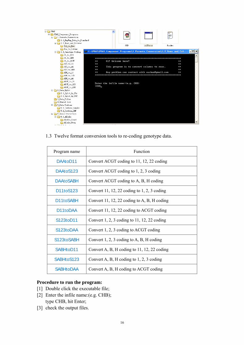
1.3 Twelve format conversion tools to re-coding genotype data.
Program name Function
DAAtoD11 Convert ACGT coding to 11, 12, 22 coding
DAAtoS123 Convert ACGT coding to 1, 2, 3 coding
DAAtoSABH Convert ACGT coding to A, B, H coding
D11toS123 Convert 11, 12, 22 coding to 1, 2, 3 coding
D11toSABH Convert 11, 12, 22 coding to A, B, H coding
D11toDAA Convert 11, 12, 22 coding to ACGT coding
S123toD11 Convert 1, 2, 3 coding to 11, 12, 22 coding
S123toDAA Convert 1, 2, 3 coding to ACGT coding
S123toSABH Convert 1, 2, 3 coding to A, B, H coding
SABHtoD11 Convert A, B, H coding to 11, 12, 22 coding
SABHtoS123 Convert A, B, H coding to 1, 2, 3 coding
SABHtoDAA Convert A, B, H coding to ACGT coding
Procedure to run the program: [1] Double click the executable file; [2] Enter the infile name:(e.g. CHB);
type CHB, hit Enter; [3] check the output files.
16
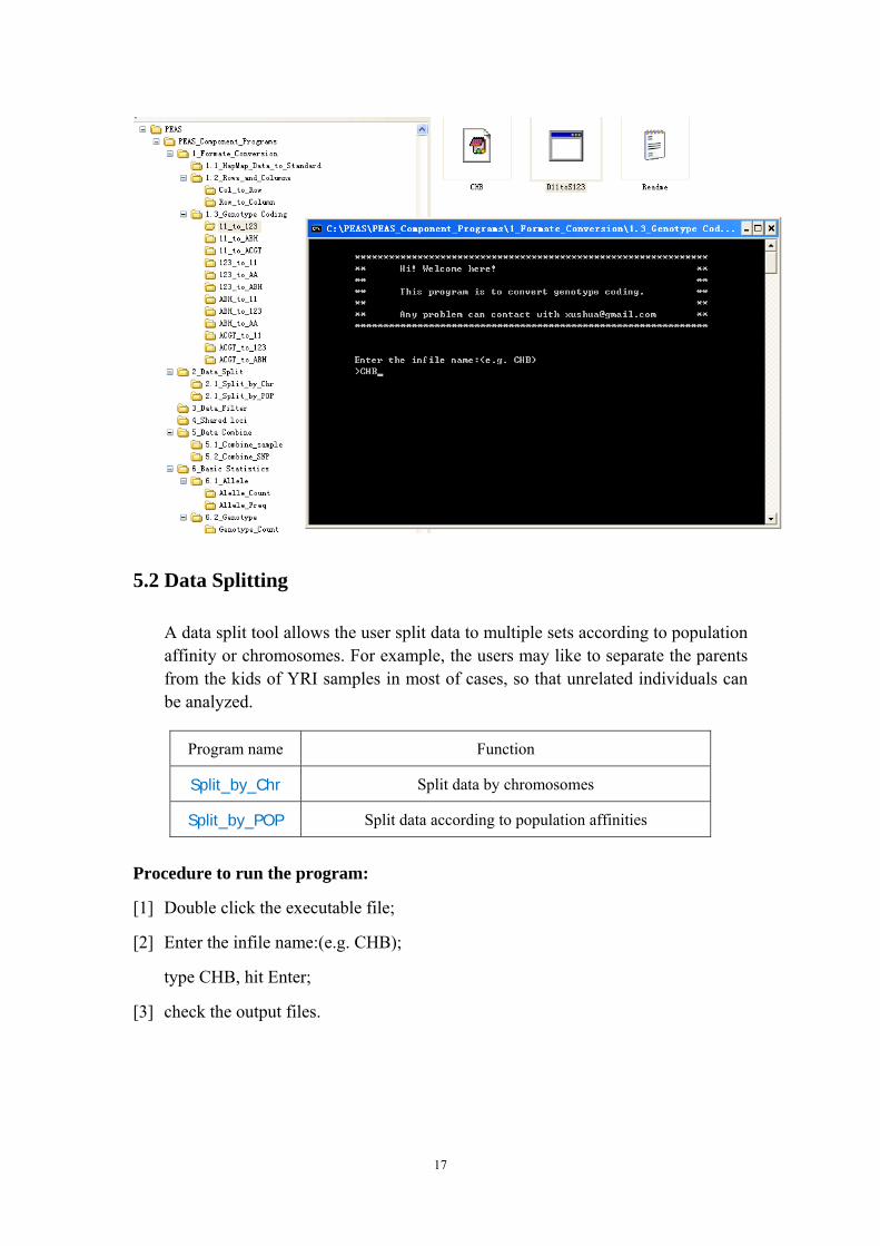
5.2 Data Splitting
A data split tool allows the user split data to multiple sets according to population affinity or chromosomes. For example, the users may like to separate the parents from the kids of YRI samples in most of cases, so that unrelated individuals can be analyzed.
Program name Function
Split_by_Chr Split data by chromosomes
Split_by_POP Split data according to population affinities
Procedure to run the program:
[1] Double click the executable file;
[2] Enter the infile name:(e.g. CHB);
type CHB, hit Enter;
[3] check the output files.
17

5.3 Data Filtering
A filter tool allows the user filter data by MAF, missing data proportion and
HWE states.
Program name Function
filter Filter data by MAF, missing data proportion and HWE
Procedure to run the program:
[1] Double click the executable file; [2] Enter the chromosome name (eg. chr1; chr2; ....chrX,chrY):
type: chr22, hit Enter [3] Enter the population name (eg. CHB):
type: CHB, hit Enter [4] Enter sample size : (here for CHB is 84)
type:84, hit Enter [5] Enter extra column : (e.g. 0)
type:0, hit Enter [6] Do you want missing data filter on (0 for no;1 for yes) :
type:1, hit Enter [7] Do you want MAF filter on (0 for no;1 for yes) :
type:1, hit Enter
18

[8] Do you want HWE filter on (0 for no;1 for yes) : type:1, hit Enter
[9] Enter Threshold for missing data filter (e.g. 0.05): type:0.05, hit Enter
[10] Enter Threshold for MAF filter (e.g. 0.05): type:0.05, hit Enter
[11] Enter Threshold for HWE filter(0.001,0.005,0.01,0.05): type: 0.01, hit Enter
[12] Do you want Data for each Loci : (0 for no;1 for yes) type:1, hit Enter
[13] check the output files.
19

5.4 Consensus Markers
A consensus data tool allows the users obtain the consensus data for multiple
population samples or different resources. The program integrates data according
to the information of SNP ID, chromosome, physical position, strand (+/-).
Program name Function
Shared_loci To obtain the consensus data for multiple population samples
Procedure to run the program: [1] Double click the executable file; [2] Enter the infile name:(e.g. 2pops);
type: 2pops, hit Enter; [3] check the output files.
5.5 Data integration
A data integrate tool allows the user integrate multiple data sets by samples or by
chromosomes or by both. For example, people may like to integrate data sets
20

from different population samples when they perform fastPHASE analysis or
STRUCTURE analysis.
Program name Function
Combine_sample To combine data for multiple population samples
Combine_snp To combine data for different SNP markers
Procedure to run the program:
[1] Double click the executable file;
[2] Enter the infile name:(e.g. 4pops);
type: 4pops, hit Enter;
[3] check the output files.
5.6 Basic Statistics
Tools to allow the user calculate allele frequency and genotype frequency,
examine the HWE state of each locus.
21

Program name Function allele_count To conunt number of alleles for each SNP allele_freq To calculate allele frequency for each SNP
genotype_count To conunt number of genotypes for each SNP genotype_freq To calculate genotype frequency for each SNP
hwe To test HWE for each SNP
Procedure to run the program: [1] Double click the executable file; [2] Enter the infile name:(e.g. CHB);
type: CHB, hit Enter; [3] check the output files.
5.7 Data Sampling
A sampling tool allows the user sample subsets of data by markers.
Program name Function
SNP_Sampler
To sample subsets of data by markers, there are several options, sub-datasets can be generated by random sampling (bootstraping), or by setting inter-marker distance, or by setting a paticular heterozygosity, or by setting both inter-marker distance and heterozygosity.
22
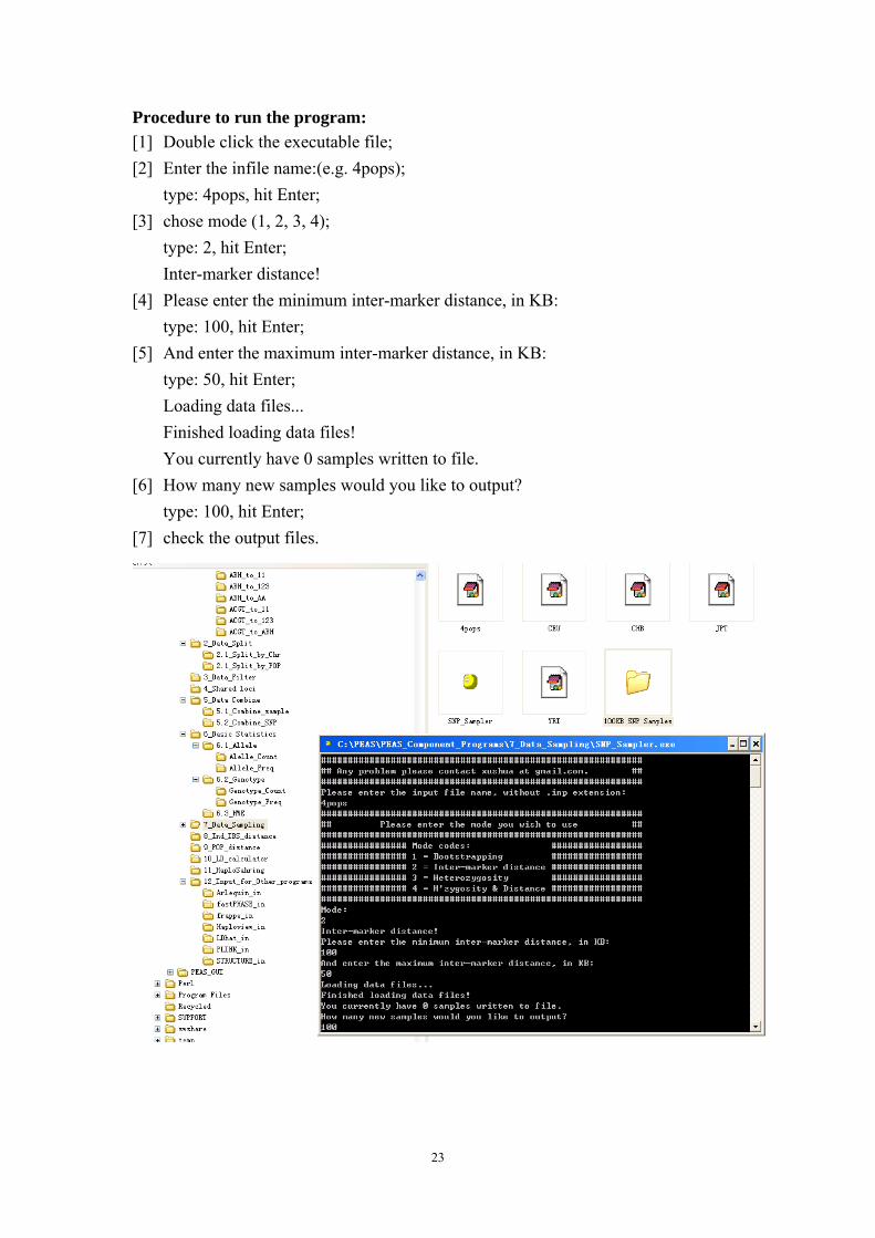
Procedure to run the program: [1] Double click the executable file; [2] Enter the infile name:(e.g. 4pops);
type: 4pops, hit Enter; [3] chose mode (1, 2, 3, 4);
type: 2, hit Enter; Inter-marker distance!
[4] Please enter the minimum inter-marker distance, in KB: type: 100, hit Enter;
[5] And enter the maximum inter-marker distance, in KB: type: 50, hit Enter; Loading data files... Finished loading data files! You currently have 0 samples written to file.
[6] How many new samples would you like to output? type: 100, hit Enter;
[7] check the output files.
23

5.8 Individual Distance
A program allows the user calculate allele sharing distance between each pair of
individuals.
Program name Function
Ind_dis_wBootStrap
This program will generate multiple distance
matrixes by bootstrapping the loci, and provides
the output files that can be read by MEGA
(Kumar, Tamura et al. 2004) and PHYLIP
(Felsenstein 1989) programs for further
processing.
Procedure to run the program: [1] Double click the executable file; [2] Enter the infile name:(e.g. 4pops);
type: 4pops, hit Enter; [3] check the output files.
24
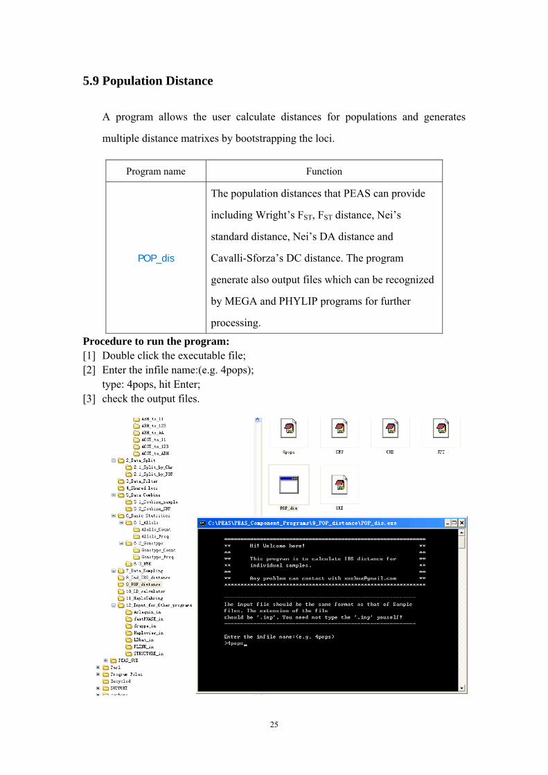
5.9 Population Distance
A program allows the user calculate distances for populations and generates
multiple distance matrixes by bootstrapping the loci.
Program name Function
POP_dis
The population distances that PEAS can provide
including Wright’s FST, FST distance, Nei’s
standard distance, Nei’s DA distance and
Cavalli-Sforza’s DC distance. The program
generate also output files which can be recognized
by MEGA and PHYLIP programs for further
processing.
Procedure to run the program: [1] Double click the executable file; [2] Enter the infile name:(e.g. 4pops);
type: 4pops, hit Enter; [3] check the output files.
25

5.10 LD calculator
A program allows the user calculate the two most commonly used LD statistics
(r2 and |D’|) and generate LD distribution report files which can be used to plot in
MS Excel. This feature is especially useful for very large data set with huge
number of SNP sites.
Program name Function
Pairwise_LD
To calculate the two most commonly used LD
statistics (r2 and |D’|). It can handle data from
multiple population samples and chromosomes. A
summary statistics table will be generated.
Procedure to run the program: [1] Double click the executable file; [2] Enter the infile name:(e.g. 4pops);
type: 4pops, hit Enter; [3] check the output files.
26
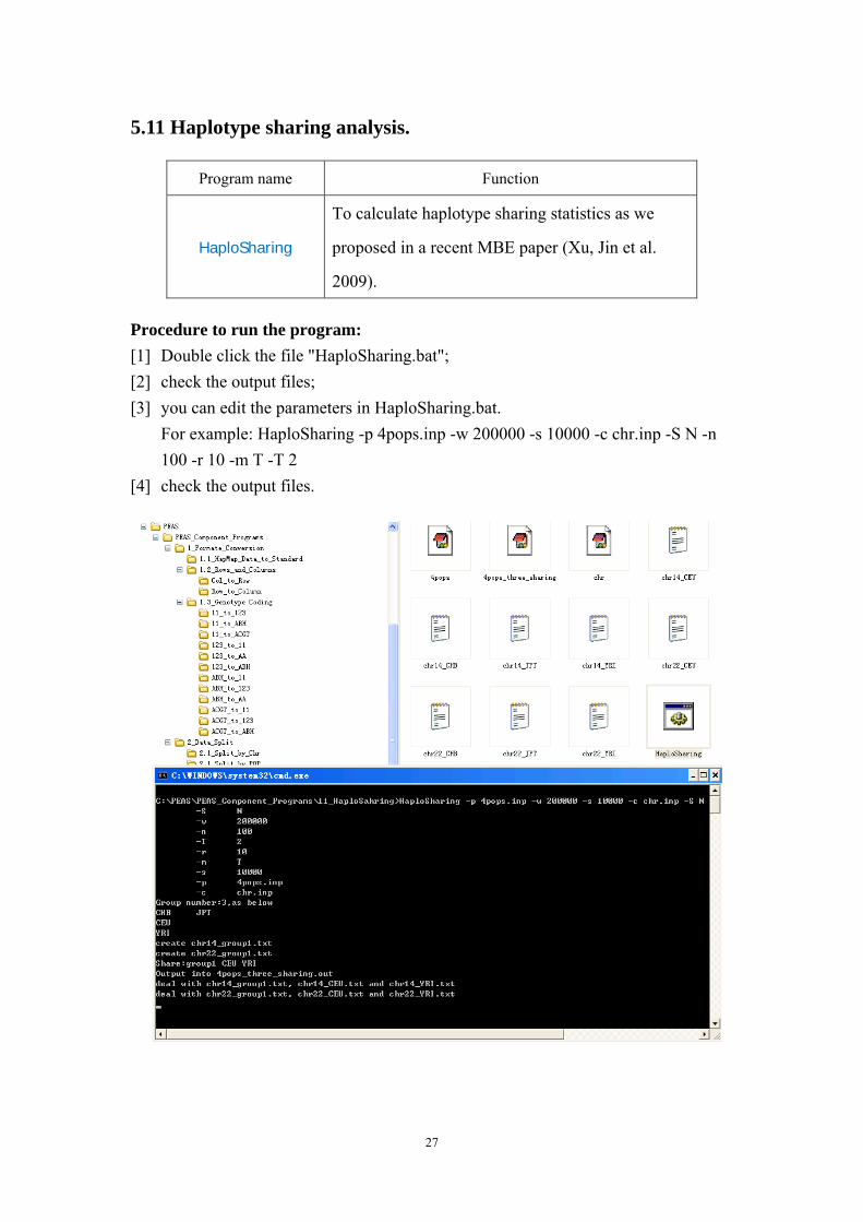
5.11 Haplotype sharing analysis.
Program name Function
HaploSharing
To calculate haplotype sharing statistics as we
proposed in a recent MBE paper (Xu, Jin et al.
2009).
Procedure to run the program: [1] Double click the file "HaploSharing.bat"; [2] check the output files; [3] you can edit the parameters in HaploSharing.bat.
For example: HaploSharing -p 4pops.inp -w 200000 -s 10000 -c chr.inp -S N -n 100 -r 10 -m T -T 2
[4] check the output files.
27

5.12 Other Software Input
A serious of tools to provide the user input files for many popular softwares
which include fastPHASE, PHASE, STRUCTURE, Haploview, Arlequin, LDhat
and PLINK.
Program name Function Arlequin_in To generate input file for Arleauin analysis
fastPHASE_in To generate input file for fastPHASE analysis frappe_in To generate input file for frappe analysis
Haploview_in To generate input file for Haploview analysis LDhat_in To generate input file for LDHat analysis PLINK_in To generate input file for PLINK analysis
STRUCTURE_in To generate input file for STRUCTURE analysis Procedure to run the program: [1] Double click the executable file; [2] Enter the infile name:(e.g. 4pops);
type: 4pops, hit Enter; [3] check the output files.
28

6 Functions in GUI
6.1 Basic data format conversion tools.
PEAS are able to transform all the 8 formats mentioned above from one the user
supplied to all the other seven ones. However, to use PEAS to do further analysis, we
recommend user convert their data into the standard format (with ABHU coding for
all possible genotypes for each SNP), because this format is easy to be handled by all
the program components in PEAS package.
6.1.1 HapMap data to Standard format
We provide a special tool for converting HapMap data format to our standard
format, as shown in the following snapshots.
29

6.1.2 Two format conversion tools to transpose data between columns and rows.
Since in most occasions the number of SNPs is much larger than that of
individual samples, the common format of SNP data is markers in rows and
individuals in colums, such as those in HapMap database. There are also many
software using pedgree-like format as input, such as PLINK, EIGENSOFT etc.
We provided a tool to convert data between rows and columns, as shown in the
following snapshots.
6.1.3 Genotype coding transformation
Genotypes of a SNP can be coded as either characters or numbers. As data from
different sources could have different coding schemes, we provide a tool to do
30

conversion between these different genetype codings. These include the following
possible conversions: ACGT to 1122; ACGT to ABH; ACGT to 123; 1122 to ACGT;
1122 to ABH; 1122 to 123; ABH to ACGT; ABH to 1122; ABH to 123.
6.2 Data split
6.2.1 Split data by samples
In some cases, data of all the samples may stored in one single file, if the user want to
separate certain group samples, such as separate kids from parents, as YRI and CEU
in HapMap data, or separate samples of one population from the other populations, as
31

CHB+JPT data file in HapMap data. PEAS reads one file with sample information
that the user defined, then separate data by sample groups that the user defined.
The structure for sample information file can be represented as follows:
NumberOfIndividuals
NumberOfExtraColumns
NumberOfGroups
GroupIndicator GroupName
GroupIndicator GroupName
…
GroupIndicator GroupName
SampleNumber GroupIndicator
SampleNumber GroupIndicator
…
SampleNumber GroupIndicator
Where the quantities above are as follows:
1. NumberOfIndividuals An integer specifying the number of individuals who
have been genotyped. It is often the total sample size in the original data file.
2. NumberOfExtraColumns An integer specifying the number of extra columns
which is relative to the standard format of genotype file. It is actually the number
of columns, if any, between the strand information (the fifth column) and
genotype data (the sixth column without extra columns).
3. NumberOfGroups An integer specifying the number of groups that all the
samples will be divided into.
4. GroupIndicator An integer will be taken as indicator of group, the number of
GroupIndicators must be the same as the number of groups, i.e. the total
number of GroupIndicators used must be NumberOfGroups.
5. GroupName A string indicating the name of group, this is also used to name the
files that store the data of this group samples.
32
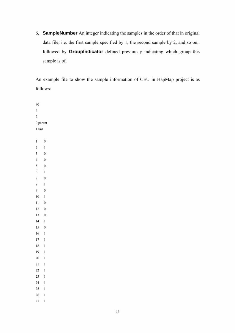
6. SampleNumber An integer indicating the samples in the order of that in original
data file, i.e. the first sample specified by 1, the second sample by 2, and so on.,
followed by GroupIndicator defined previously indicating which group this
sample is of.
An example file to show the sample information of CEU in HapMap project is as
follows:
90
6
2
0 parent
1 kid
1 0
2 1
3 0
4 0
5 0
6 1
7 0
8 1
9 0
10 1
11 0
12 0
13 0
14 1
15 0
16 1
17 1
18 1
19 1
20 1
21 1
22 1
23 1
24 1
25 1
26 1
27 1
33

28 1
29 1
30 1
31 1
32 0
33 0
34 0
35 0
36 0
37 0
38 0
39 0
40 0
41 0
42 0
43 0
44 0
45 0
46 0
47 0
48 0
49 0
50 0
51 0
52 0
53 0
54 0
55 0
56 0
57 0
58 0
59 0
60 0
61 0
62 0
63 0
64 1
65 0
66 0
67 1
68 0
69 0
70 1
71 1
72 0
34
73 0
74 0
75 0
76 1
77 1
78 0
79 0
80 0
81 0
82 1
83 1
84 0
85 0
86 0
87 0
88 1
89 0
90 0
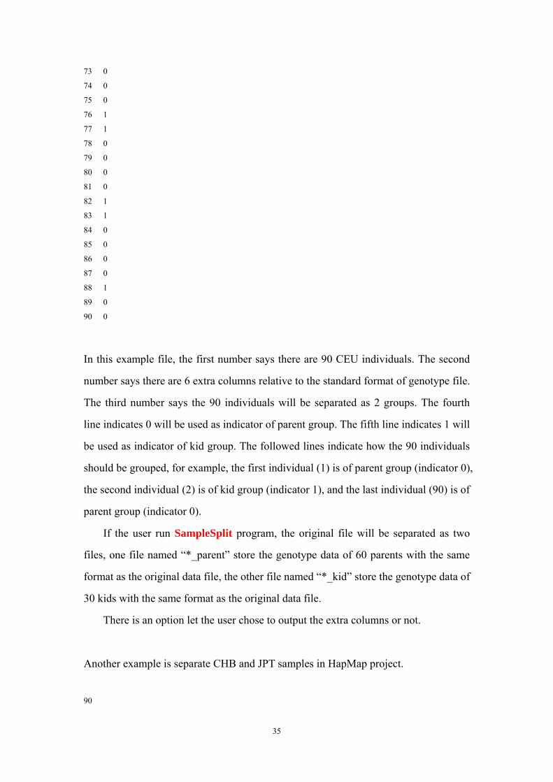
In this example file, the first number says there are 90 CEU individuals. The second
number says there are 6 extra columns relative to the standard format of genotype file.
The third number says the 90 individuals will be separated as 2 groups. The fourth
line indicates 0 will be used as indicator of parent group. The fifth line indicates 1 will
be used as indicator of kid group. The followed lines indicate how the 90 individuals
should be grouped, for example, the first individual (1) is of parent group (indicator 0),
the second individual (2) is of kid group (indicator 1), and the last individual (90) is of
parent group (indicator 0).
If the user run SampleSplit program, the original file will be separated as two
files, one file named “*_parent” store the genotype data of 60 parents with the same
format as the original data file, the other file named “*_kid” store the genotype data of
30 kids with the same format as the original data file.
There is an option let the user chose to output the extra columns or not.
Another example is separate CHB and JPT samples in HapMap project.
90
35
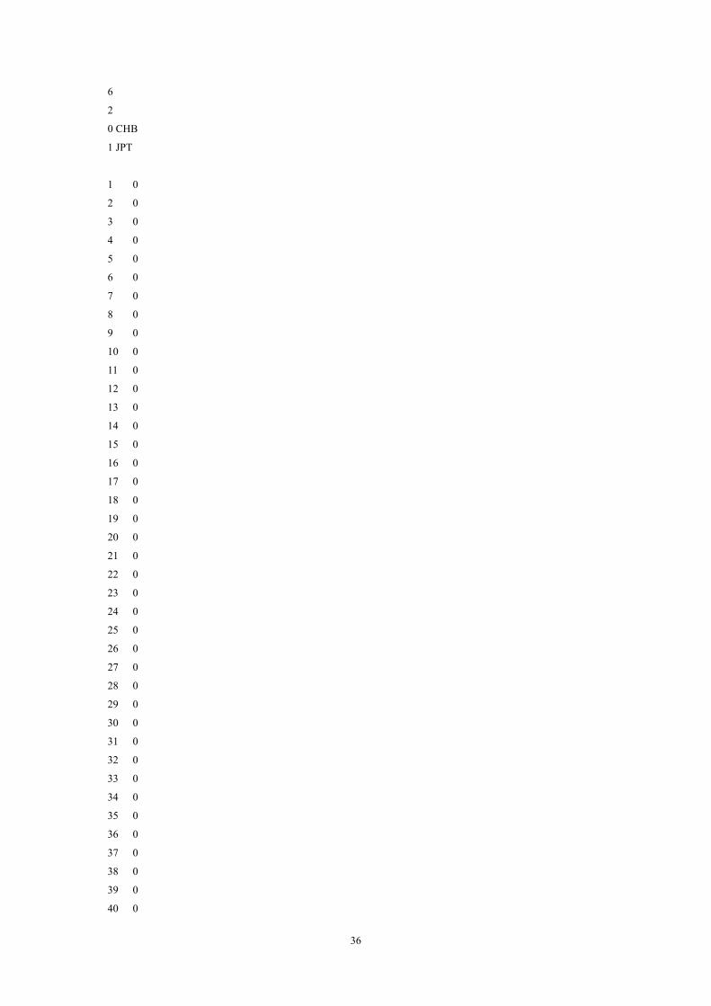
6
2
0 CHB
1 JPT
1 0
2 0
3 0
4 0
5 0
6 0
7 0
8 0
9 0
10 0
11 0
12 0
13 0
14 0
15 0
16 0
17 0
18 0
19 0
20 0
21 0
22 0
23 0
24 0
25 0
26 0
27 0
28 0
29 0
30 0
31 0
32 0
33 0
34 0
35 0
36 0
37 0
38 0
39 0
40 0
36

41 0
42 0
43 0
44 0
45 0
46 1
47 1
48 1
49 1
50 1
51 1
52 1
53 1
54 1
55 1
56 1
57 1
58 1
59 1
60 1
61 1
62 1
63 1
64 1
65 1
66 1
67 1
68 1
69 1
70 1
71 1
72 1
73 1
74 1
75 1
76 1
77 1
78 1
79 1
80 1
81 1
82 1
83 1
84 1
85 1
37

86 1
87 1
88 1
89 1
90 1
In this example file, the first number says there are 90 individuals. The second
number says there are 6 extra columns relative to the standard format of genotype file.
The third number says the 90 individuals will be separated as 2 groups. The fourth
line indicates 0 will be used as indicator of CHB group. The fifth line indicates 1 will
be used as indicator of JPT group. The followed lines indicate how the 90 individuals
should be grouped, for example, the first 45 individual (1 to 45) is of CHB group
(indicator 0), and the rest 45 individual (46 to 90) is of JPT group (indicator 1).
If the user run SampleSplit program, the original file will be separated as two
files, one file named “*_CHB” store the genotype data of 45 CHB individuals with
the same format as the original data file, the other file named “*_JPT” store the
genotype data of 45 JPT individuals with the same format as the original data file.
Note 5: PEAS can split the samples to any number of groups, as defined by the user
in the information file, but to make this split to be meaningful, the number of groups
should be no more than the total number of individuals, i.e. the maximal number of
groups should be smaller than the total sample size.
38

6.2.2 Split data by markers
PEAS can also split data by chromosome information, so that data of each single
chromosome can be analyzed separately.
39
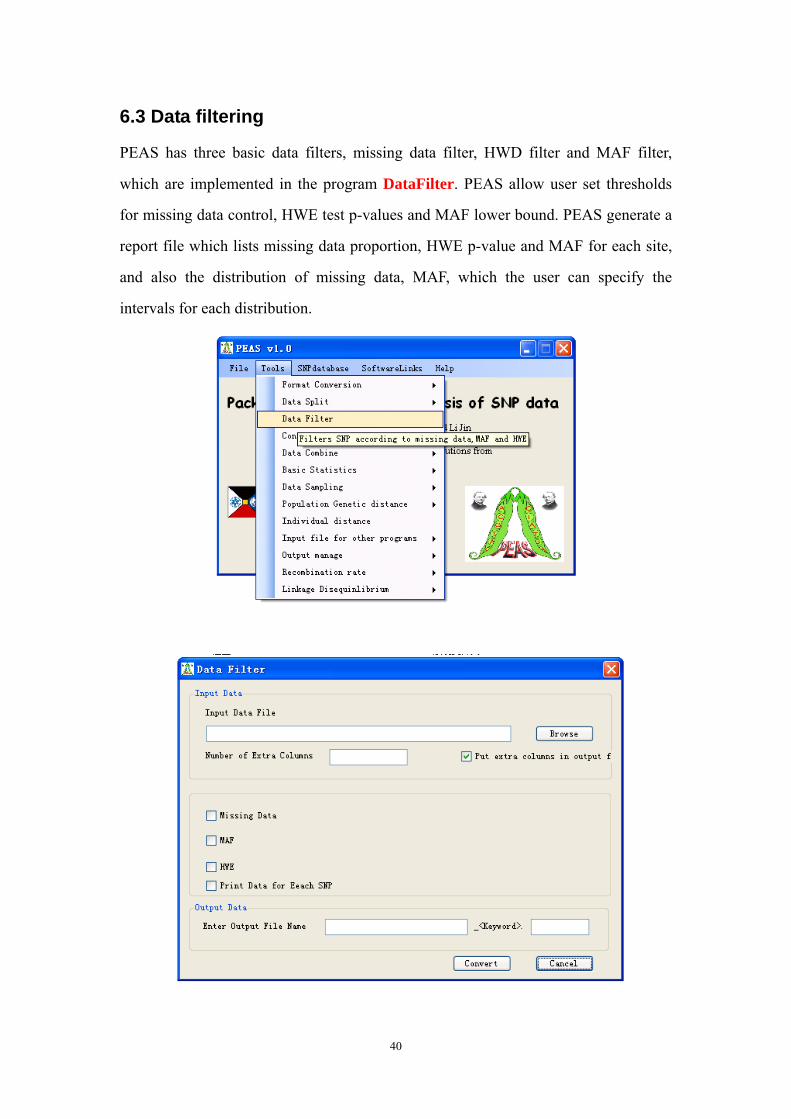
6.3 Data filtering
PEAS has three basic data filters, missing data filter, HWD filter and MAF filter,
which are implemented in the program DataFilter. PEAS allow user set thresholds
for missing data control, HWE test p-values and MAF lower bound. PEAS generate a
report file which lists missing data proportion, HWE p-value and MAF for each site,
and also the distribution of missing data, MAF, which the user can specify the
intervals for each distribution.
40

6.4 Search shared loci
For many purposes of data analysis, it is necessary to use the shared loci among
multiple populations. PEAS provides a program SharedLociSearcher to search the
shared loci among populations. The user should provide a file specify some basic
information of the populations, the structure of the file is as follows:
NumberOfPopulations
PopulationName ExtraColumns SampleSize
…
PopulationName ExtraColumns SampleSize
For example, the following file says there are 2 populations need to be searched
shared loci, CEU is the name of the first population, the data file has 0 (no) extra
column, the sample size of CEU is 90, YRI is the name of the second population, the
data file has 0 (no) extra column, the sample size of YRI is 90.
2
CEU 0 90
YRI 0 90
41

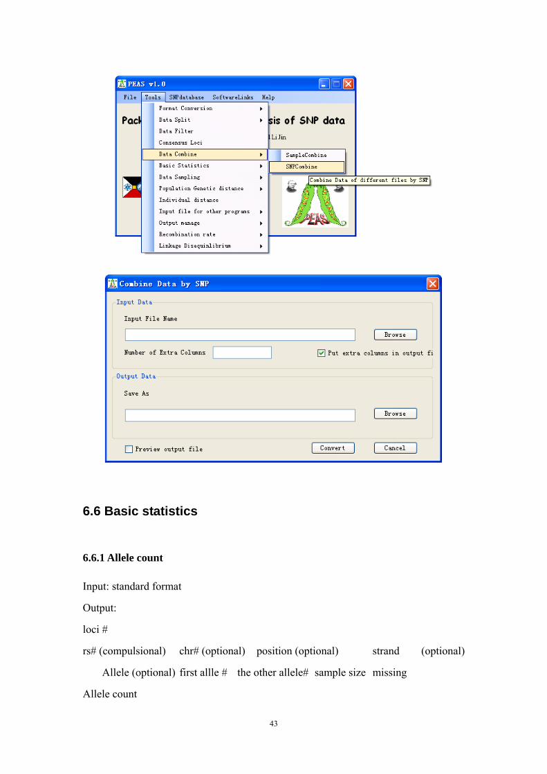
6.5 Data combination
As the princinple of data split, PEAS can also combine data from different individuals,
or from different SNP markers.
42
6.6 Basic statistics
6.6.1 Allele count
Input: standard format
Output:
loci #
rs# (compulsional) chr# (optional) position (optional) strand (optional)
Allele (optional) first allle # the other allele# sample size missing
Allele count
43

6.6.2 Allele frequency
rs# (compulsional) chr# (optional) position (optional) strand (optional)
Allele (optional) first alle freq the other allele freq minor allele freq (MAF)
sample size missing (0.01)
Allele frequency
44
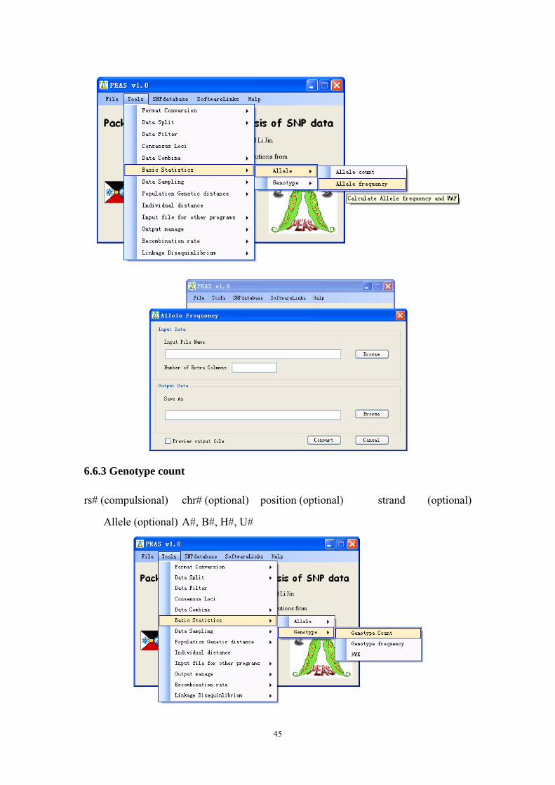
6.6.3 Genotype count
rs# (compulsional) chr# (optional) position (optional) strand (optional)
Allele (optional) A#, B#, H#, U#
45

6.6.4 Genotype frequency
rs# (compulsional) chr# (optional) position (optional) strand (optional)
Allele (optional) A_freq, B_freq, H_freq, U_freq
6.6.5 Hardy-Weinberg equilibrium (p-value threshold, 0.05)
rs# (compulsional) chr# (optional) position (optional) strand (optional)
Allele (optional) Observed Heterozygosity Expected Heterozygosity X2 p-value
E/D
In some studies, people prefer to provide another format of genotype data. This
For many purposes, allele frequencies provide enough information. PEAS provides a
program AlleleFreq caluculate allele frequency for multiple populations and
generates some basic information such as MAF and missing data proportion for each
SNP in each population.
46

6.7 Population genetic distances
Many people are interested in the genetic differentiation of populations, some genetic
distances are used to describe the genetic difference between populations, such as FST,
Nei’s standard distance, Nei’s DA distance, F*ST distance and Cavalli-Sforza’s dC
distance. PEAS provides a program POPdis to calculate those commonly used
distances. PEAS generates distance matrix as MEGA format so that the results can be
directly used to reconstruct phylogenetic trees. PEAS also does bootstrapping and
generate Phylip format files and the results can be read and analyzed by Neighbor
program and Consence program in Phylip package.
The formula used to calculate the distances are as follows:
6.7.1 Estimates of FST
Unbiased estimates of FST were calculated as described by Weir and Hill
2002(Weir and Hill 2002). Suppose we have i subpopulations (where i = 1,…, r), we
denote sample allele frequency as ip~ , and denote the average frequency over samples
as ip . The allele in the ith sample is denoted by . If there are alleles
sampled from the of
jth ijx in
ith r populations:
47

∑=
=in
jij
ii x
np
1
1~
∑∑ =
=r
iii
ii
pnn
p1
~1
The observed mean square errors for loci within populations are denoted by MSG:
( )( )ii
r
iir
ii
ppnn
MSG ~1~
1
1
1
−−
= ∑∑=
The observed mean square errors for between populations are denoted by MSP:
( )2~1
1 ppnr
MSP i
r
ii −
−= ∑
Then FST can be estimated as follows:
( )MSGnMSPMSGMSPF
cST 1−+
−=
Where is the average sample size across samples that also incorporates and
corrects for the variance in sample size over subpopulations:
cn
⎟⎟
⎠
⎞
⎜⎜
⎝
⎛−
−=
∑∑∑
=
=
=r
i i
r
i is
iic
n
nn
rn
1
12
111
Because negative values of FST do not have biological interpretation, we set negative
values of FST=0.0.
6.7.2 F*ST Distance
According to Latter(Latter 1972),
( )XY
XYYX
ST J
JJJF ˆ1
ˆˆˆ21
*
−
−+=
where , and are the unbiased estimates of average of ,
and for all loci respectively. For a single locus, the unbiased estimates of
, and are:
XJ
i yx
∑
YJ
2i
XYJ
∑ i yx
∑ 2ix ∑ 2
iy
∑ i
2i y∑ x i
48

12
1ˆ2ˆ
2
−
−=
∑X
iX
X m
Xmj
12
1ˆ2ˆ
2
−
−=
∑Y
iY
Y m
Ymj
∑= iiXY YXj ˆˆˆ
where mX and mY are the number of diploids sampled from population X and Y
respectively, and are allele frequencies in samples(Nei 1987). Therefore, ,
and are the averages of , and in all loci.
ix iy XJ
YJ XYJ Xj Yj XYj
6.7.3 Nei’s Standard Distance
According to Nei(Nei 1972),
)ln(ID −=
where
YX
XY
JJ
JIˆˆ
ˆ=
where , and are the unbiased estimates of average of ,
and for all loci respectively. For a single locus, the unbiased estimates of
, and are:
XJ
i yx
∑
YJ
2i
XYJ
∑ i yx
∑ 2ix ∑ 2
iy
∑ i
2i y∑ x i
12
1ˆ2ˆ
2
−
−=
∑X
iX
X m
Xmj
12
1ˆ2ˆ
2
−
−=
∑Y
iY
Y m
Ymj
∑= iiXY YXj ˆˆˆ
where mX and mY are the number of diploids sampled from population X and Y
49
respectively, and are allele frequencies in samples(Nei 1987). Therefore, ,
and are the averages of , and in all loci.
ix iy XJ
YJ XYJ Xj Yj XYj
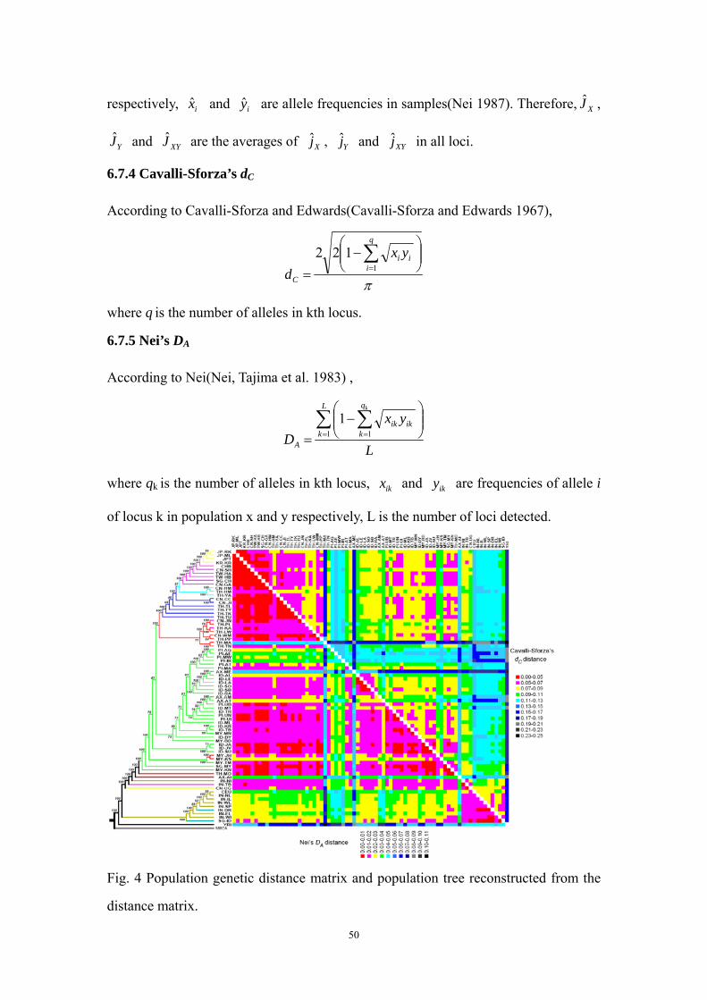
6.7.4 Cavalli-Sforza’s dC
According to Cavalli-Sforza and Edwards(Cavalli-Sforza and Edwards 1967),
π
⎟⎟⎠
⎞⎜⎜⎝
⎛−
=∑=
q
iii
C
yxd 1
122
where q is the number of alleles in kth locus.
6.7.5 Nei’s DA
According to Nei(Nei, Tajima et al. 1983) ,
L
yxD
L
k
q
kikik
A
k
∑ ∑= =
⎟⎟⎠
⎞⎜⎜⎝
⎛−
= 1 11
where qk is the number of alleles in kth locus, ikx and are frequencies of allele i
of locus k in population x and y respectively, L is the number of loci detected.
iky
Fig. 4 Population genetic distance matrix and population tree reconstructed from the
distance matrix.
50

6.7.6 Output distance matrix for MEGA and PHYLIP analysis
All the distance matrices calculated by PEAS are converted to MEGA and PHYLIP
input format, so that phylogenetic analysis could be done easily.
6.7.7 Bootstrapping for distance calculation
As for trees, the best check of the validity of the conclusions is their independence
from the markers employed: that is, their reproducibility with different sets of
markers.
6.8 Individual genetic distances
PEAS also provide a program Indis to calculate the genetic distance between
individuals.
6.8.1 Allele sharing distance
We used an allele sharing distance(Mountain and Cavalli-Sforza 1997) as the genetic
distance between individuals and reconstructed an individual tree to explore their
relationship using Neighbor-Joining algorithm(Saitou and Nei 1987). Consider one
biallelic SNP; there are three possible genotypes, AA, Aa, and aa. The genetic
distances between individuals were calculated as follow:
∑=
=l
kkijij d
lD
1
1 ,
where l is the number of loci for which both individuals have been tested, and dkij=0 if
individual i and individual j have identical genotypes at locus k (e.g., AA:AA or
Aa:Aa or aa:aa), dkij=0.5 if individual i and individual j have one one allele identical
one allele different (e.g., AA:Aa or aa:Aa), and dkij=1.0 if individual i and individual j
have no alleles in common (e.g., AA:aa).
51

Fig. 5 Individual tree of 270 HapMap samples, red branches indicate CHB and JPT samples,
blue branches indicate CEU samples and black branches indicate YRI samples.
52

6.9 Input files for other programs
As described in PEAS component programs, PEAS can generate input file for the
following popular computer programs which have been used frequently in studies on
human population genetics.
6.9.1 Format input files for PHASE
PEAS provides a program PHASEin to format the genotype data to the input file for
PHASE (Stephens, Smith et al. 2001) program.
6.9.2 Format input files for fastPHASE
PEAS also provides a program fastPHASEin to format the genotype data to the input
file for fastPHASE (Scheet and Stephens 2006) program.
6.9.3 Format input files for STRUCTURE
PEAS also provides a program STRUCTUREin to format the genotype data to the
input file for STRUCTURE (Falush, Stephens et al. 2003) program.
6.9.4 Format input files for Arlequin
PEAS also provides a program ArlequinIn to format the genotype data to the input
53

file for Arlequin (Excoffier and Schneider 2005) program.
6.9.5 Format input files for Haploview
PEAS also provides a program HaploviewIn to format the genotype data to the input
file for Haploview (Barrett, Fry et al. 2005) program.
6.9.6 Format input files for LDhat
PEAS also provides a program LDhatIn to format the genotype data to the input file
for LDhat (McVean, Myers et al. 2004) program.
6.10 Linkage Disequilibrium
6.10.1 Measures of Linkage Disequilibrium
Hedrick (Hedrick 1987) has reviewed the numerous measures of linkage
disequilibrium. In his review, Hedrick demonstrates the conditions under which the
measures, or at least a subset thereof, are highly correlated. Devilin and Risch (Devlin
and Risch 1995) compared linkage disequilibrium for fine-scale mapping.
Consider two loci, A and B, each locus having two alleles: A1, A2 of locus A, B1, B2 of
locus B respectively. The layout and notation of the 2 × 2 table from a sample from
the population are given in Table 1. In Table 1, p11, p12, p21, p22 denote the observed
frequencies of haplotype A1B1, A1B2, A2B1, A2B2, p1+, p2+, p+1, p+2 denote the
frequencies of allele A1, A2, B1, B2.
Table 1 Layout and Notation for Sample Haplotype Frequencies in a 2 × 2 Table
marker B1 B2
A1 p11 p12 p1+
A2 p21 p22 p2+
p+1 p+2 1
Naturally the p’s are only sample estimates of some underlying unknown parameters,
denoted by p’s. We use p’s in the definitions that follow, with the understanding that
54

these unknown quantities are estimated from the observed sample quantities.
The basic component of many measures of disequilibrium is the difference between
the observed and the expected (under independence) number of haplotypes bearing
the A1 and the B1 allele or its equivalent expressions:
11 1 1
22 2 2
12 1 2
21 2 1
11 22 12 21
DD
DD
D
π π ππ π ππ π ππ π π
π π π π
+ +
+ +
+ +
+ +
= −= −= − += − += −
, the corresponding estimation is
11 1 1
22 2 2
12 1 2
21 2 1
11 22 12 21
p p pp p p
D p p pp p p
p p
DD
D p pD
+ +
+ +
+ +
+ +
= −= −= − += − += −
.
Although the measure D captures the intuitive concept of LD, its numerical value
is of little use for measuring the strength of and comparing levels of LD. This is due
to the dependence of D on allele frequencies. As a result, several alternative measures
based on D have been devised (Devlin and Risch 1995).
According to Hill and Weir (Hill and Weir 1994), the most frequently used
measure of disequilibrium is the square of standardized measure
2121
21122211
++++
−=Δ
ππππππππ
,
or ∆2. ∆ is commonly squared to remove the arbitrary sign introduced when the
marker alleles are labeled.
Another common measure, introduced by Lewontin (Lewontin 1964), is defined
as
( )
( )⎪⎪⎩
⎪⎪⎨
⎧
<−
>−
=
++++
++++
0,min
0,min'
2211
21122211
2121
21122211
D
DD
ππππππππππππ
ππππ
, where
211222111221211222221111 ππππππππππππππππ −=−−=−−=−=−= ++++++++D .
7 How to cite this program
Shuhua Xu, Sanchit Guputa and Li Jin. 2010. PEAS: A Package for Elementary
Analysis of SNP Data. Chinese Academy of Sciences and Max Planck Society
(CAS-MPG) Partner Institute for Computational Biology, Shanghai Institutes for
55
Biological Sciences, Chinese Academy of Sciences, Shanghai 200031, China.
8 References
Barrett, J. C., B. Fry, et al. (2005). "Haploview: analysis and visualization of LD and haplotype
maps." Bioinformatics 21(2): 263-5. Cavalli-Sforza, L. L. and A. W. Edwards (1967). "Phylogenetic analysis. Models and estimation
procedures." Am J Hum Genet 19(3): Suppl 19:233+. Devlin, B. and N. Risch (1995). "A comparison of linkage disequilibrium measures for fine-scale
mapping." Genomics 29(2): 311-22. Excoffier, L. and S. Schneider (2005). "Arlequin ver. 3.0: An integrated software package for
population genetics data analysis." Evolutionary Bioinformatics Online 1: 47-50. Falush, D., M. Stephens, et al. (2003). "Inference of population structure using multilocus genotype
data: linked loci and correlated allele frequencies." Genetics 164(4): 1567-87. Felsenstein, J. (1989). "PHYLIP--Phylogeny Inference Package (Version 3.2)." Cladistics 5: 164-166. Hedrick, P. W. (1987). "Genetic bottlenecks." Science 237(4818): 963. Hill, W. G. and B. S. Weir (1994). "Maximum-likelihood estimation of gene location by linkage
disequilibrium." Am J Hum Genet 54(4): 705-14. Kumar, S., K. Tamura, et al. (2004). "MEGA3: Integrated software for Molecular Evolutionary
Genetics Analysis and sequence alignment." Brief Bioinform 5(2): 150-63. Latter, B. D. (1972). "Selection in finite populations with multiple alleles. 3. Genetic divergence with
centripetal selection and mutation." Genetics 70(3): 475-90. Lewontin, R. C. (1964). "The Interaction of Selection and Linkage. Ii. Optimum Models." Genetics 50:
757-82. McVean, G. A., S. R. Myers, et al. (2004). "The fine-scale structure of recombination rate variation in
the human genome." Science 304(5670): 581-4. Mountain, J. L. and L. L. Cavalli-Sforza (1997). "Multilocus genotypes, a tree of individuals, and
human evolutionary history." Am J Hum Genet 61(3): 705-18. Nei, M. (1972). "Genetic distance between populations." Am. Nat. 106: 283-292. Nei, M. (1987). Molecular evolutionary genetics. New York, Columbia University Press. Nei, M., F. Tajima, et al. (1983). "Accuracy of estimated phylogenetic trees from molecular data. II.
Gene frequency data." J Mol Evol 19(2): 153-70. Pritchard, J. K., M. Stephens, et al. (2000). "Inference of population structure using multilocus
genotype data." Genetics 155(2): 945-59. Saitou, N. and M. Nei (1987). "The neighbor-joining method: a new method for reconstructing
phylogenetic trees." Mol Biol Evol 4(4): 406-25. Scheet, P. and M. Stephens (2006). "A fast and flexible statistical model for large-scale population
genotype data: applications to inferring missing genotypes and haplotypic phase." Am J Hum Genet 78(4): 629-44.
Schneider, S., D. Roessli, et al. (2000). "Arlequin: A software for population genetics data analysis. Ver
56

57
2.000." Genetics and Biometry Lab, Dept. of Anthropology, University of Geneva. Stephens, M., N. J. Smith, et al. (2001). "A new statistical method for haplotype reconstruction from
population data." Am J Hum Genet 68(4): 978-89. TheInternationalHapMapConsortium (2003). "The International HapMap Project." Nature 426(6968):
789-96. TheInternationalHapMapConsortium (2005). "A haplotype map of the human genome." Nature
437(7063): 1299-320. Weir, B. S. and W. G. Hill (2002). "Estimating F-statistics." Annu Rev Genet 36: 721-50. Xu, S., W. Jin, et al. (2009). "Haplotype-sharing analysis showing Uyghurs are unlikely genetic
donors." Mol Biol Evol 26(10): 2197-206.