Embed Size (px)
Citation preview
Pedro Henrique Fonseca da Silva Diniz
A Spatio-Temporal Model for Average Speed Predictionon Roads
Dissertacao de Mestrado
Thesis presented to the Programa de Pos-Graduacao em Informatica of theDepartamento de Informatica from PUC–Rio as partial fulfilment of therequirements for the degree of Mestre em Informatica
Advisor: Prof. Helio Cortes Vieira Lopes
Rio de JaneiroAugust of 2015
Pedro Henrique Fonseca da Silva Diniz
A Spatio-Temporal Model for Average Speed Predictionon Roads
Thesis presented to the Programa de Pos-Graduacao em Informatica of theDepartamento de Informatica from PUC–Rio as partial fulfilment of therequirements for the degree of Mestre em Informatica.
Prof. Helio Cortes Vieira LopesAdvisor
Departamento de Informatica — PUC–Rio
Prof. Marco Antonio CasanovaDepartamento de Informatica — PUC–Rio
Prof. Ruy Luiz MilidiuDepartamento de Informatica — PUC–Rio
Prof. Marcelo TılioInstituto Tecgraf — PUC–Rio
Prof. Jose Eugenio LealCoordinator of the Centro Tecnico Cientıfico — PUC–Rio
Rio de Janeiro, August 21, 2015
All rights reserved
Pedro Henrique Fonseca da Silva Diniz
Pedro Henrique Fonseca da Silva Diniz holds a Bachelor’s Degree inComputer Science from the Pontifical Catholic University of Rio de Janeiro(PUC-Rio). Currently, Pedro is a senior developer at the Tecgraf Institute ofPUC-Rio, working with Big Data GIS applications specialized on GPS signalprocessing to monitor and identify moving object events through movementworkflows. His main research interests include Algorithmic Optimizations,Distributed Systems, and Machine Learning
Bibliographic dataDiniz, Pedro Henrique Fonseca da Silva
A Spatio-Temporal Model for Average Speed Prediction on Roads /Pedro Henrique Fonseca da Silva Diniz; advisor: Helio Cortes Vieira Lopes.— 2015.
75 f. : il. (color); 30 cm
1. Tese (mestrado) - Pontifıcia Universidade Catolica do Rio de Janeiro,Departamento de Informatica, 2015.
Bibliography included.
1. Informatica – Teses. 2. Spatiotemporal Modeling. 3. StatisticalLearning. 4. GPS data. I. Lopes, Helio Cortes Vieira. II. PontifıciaUniversidade Catolica do Rio de Janeiro. Departamento de Informatica. III.Tıtulo.
CDD: 510

Acknowledgments
To my parents, Carlos Alberto and Jussara Oliveira, who not only
supported me and my dreams, but also always encouraged me to do better.
Even if all fails, if I can make you happy, than it is sure worth it. To my
wife Anna Carolina, who patiently listened my ideas, gave me strength in
my weakest moments, and gave me love when I needed most. To my brother,
whose wisdom always inspired me in my life and career, and all of my family,
you guys are one of the reasons why I smile every day when I wake up. To my
advisor Helio Cortes Vieira Lopes for guiding and supporting me throughout
this work, I am really lucky to have been given an opportunity to learn from
you. To the Tecgraf Institute for sponsoring my studies and being one of the
best places a developer/researcher can work in Rio de Janeiro, without this
support the results would not have been the same. You can be certain that
you have changed a person’s life, the world is a better place with organizations
like you.
Abstract
Diniz, Pedro Henrique Fonseca da Silva; Lopes, Helio CortesVieira(Advisor) . A Spatio-Temporal Model for AverageSpeed Prediction on Roads. Rio de Janeiro, 2015. 75p. MSc.Thesis — Departamento de Informatica, Pontifıcia UniversidadeCatolica do Rio de Janeiro.
Many factors may influence a vehicle speed in a road, but two of
them are usually observed by many drivers: its location and the time of
the day. To obtain a model that returns the average speed as a function
of position and time is still a challenging task. The application of such
models can be in different scenarios, such as: estimated time of arrival,
shortest route paths, traffic prediction, and accident detection, just to cite
a few. This study proposes a prediction model based on a spatio-temporal
partition and mean/instantaneous speeds collected from historic GPS data.
The main advantage of the proposed model is that it is very simple to
compute. Moreover, experimental results obtained from fuel delivery trucks,
along the whole year of 2013 in Brazil, indicate that most of the observations
can be predicted using this model within an acceptable error tolerance.
KeywordsSpatiotemporal Modeling; Statistical Learning; GPS data.
Resumo
Diniz, Pedro Henrique Fonseca da Silva; Lopes, Helio CortesVieira . Um Modelo Espaco-Temporal para a Previsaode Velocidade Media em Estradas. Rio de Janeiro, 2015.75p. Dissertacao de Mestrado — Departamento de Informatica,Pontifıcia Universidade Catolica do Rio de Janeiro.
Muitos fatores podem influenciar a velocidade de um veıculo numa
rodovia ou estrada, mas dois deles sao observados diariamente pelos
motoristas: sua localizacao e o momento do dia. Obter modelos que
retornem a velocidade media como uma funcao do espaco e do tempo e
ainda uma tarefa desafiadora. Sao muitas as aplicacoes para esses tipos de
modelos, como por exemplo: tempo estimado de chegada, caminho mais
curto e previsao de trafico, deteccao de acidente, entre outros. Este estudo
propoe um modelo de previsao baseado em uma media espaco-temporal
da velocidade media/instantanea coletada de dados historicos de GPS. A
grande vantagem do modelo proposto e a sua simplicidade. Alem disso, os
resultados experimentais obtidos de caminhoes de entrega de combustıveis,
por todo o ano de 2013 no Brasil, indicaram que a maioria das observacoes
podem ser preditas usando esse modelo dentro de uma tolerancia de erro
aceitavel.
Palavras–chaveModelagem Espaco-Temporal; Aprendizado Estatıstico.

Contents
1 Introduction 10
2 Related Work 12
3 Preliminaries 143.1 Motivating Data 143.2 Data Preparation 173.3 Map Matching 17
4 Data Analysis 184.1 Temporal Analysis 184.2 Spatial Analysis 25
5 Spatio-Temporal Partitioning 305.1 Spatial Partitioning 305.2 Temporal Partitioning 405.3 Proposed Solution 45
6 Experiments 486.1 Experimental Setup 486.2 Evaluation Measures 486.3 Implemented Methods 496.4 Experimental Results 49
7 Conclusions and Future Works 70
8 Bibliography 72
List of figures
3.1 Piecewise linear view of the 4 routes used in this study, on a map 16
4.1 GPS signal density plot on Av. Brasil, differentiating weekendsfrom week days 20
4.2 GPS signals observations from the data as a function of space,time, and speed 24
4.3 Travel plot obtained from the data as a function of space, speedand time 29
5.1 Spatial partition quartils 355.2 Spatial segment quartil comparison 395.3 Temporal analysis of a road segment speed varying over time. 445.4 Spatio-temporal model based on instantaneous and mean speed
observations 46
6.1 Contour comparison of methods 4 and 5 on direction 1 576.2 Contour comparison of methods 4 and 5 on direction 2 616.3 Method 5 prediction error distribution analysis on direction 1 656.4 Method 5 prediction error distribution analysis on direction 2 69

List of tables
6.1 Mean Absolute Error (km/h) 526.2 Root Mean Squared Error (km/h) 526.3 Median Absolute Deviation (km/h) 526.4 Running Times (seconds) 536.5 Mean Absolute Percentage Error (ETA) 53

1Introduction
With GPS devices becoming more accessible each year, the search for a
good prediction model derived from such data is becoming a common task
(Hofmann-Wellenhof et al., 2013). However, raw GPS data comes with its
own set of problems that can also be a challenge to work with. Travel direction
is generally unknown, signal precision is, in many circumstances, unreliable,
and each device has its own transmission interval that contains no relation
with its current location, leading to irregular time and space properties.
Being a subject of general interest, a reliable model for road speed
prediction could be used to solve many of our day-to-day problems, including
traffic prediction (Fabritiis et al., 2008), estimated time of arrival (Vanajakshi
et al., 2009), shortest route paths (Derekenaris et al., 2001), and accident
detection (Kamran and Haas, 2007). Solving such problems constitutes
part of the challenges that must be overcome to implement a Smart City
(Hollands, 2008), and it is a challenging task involving the correlation study
of many factors including time, space, accidents, rain condition, vehicle type,
and many others. It remains an open question that doesn’t have a unique
answer, since each scenario generally requires a specific prediction model (a
good model for cars may not be a good model for motorcycles or buses, for
example).
While there are many models (SVR, ARIMA, ANN, and others) that
can be used to tackle this problem, most of them are focused on Travel Time
applications and are also highly dependent on real-time data, a limitation
that improves prediction accuracy, but makes them unsuitable for a future
logistic planning. A reliable model that learns from historical data and can
be used to predict speed in few months ahead is still needed.

Chapter 1. Introduction 11
By acknowledging this need, the objective of this study is to build
a reliable average speed prediction model for highways or speedways. Such
model is a function of space and time, and its input set is a collection of GPS
data. Its main idea is to build a piece-wise speed prediction model based on
segment partition of a road.
This work is organized as follows; Chapter 2 presents some of the
existing speed prediction models and attempts to classify them. The
motivational data and initial preparations are discussed in Chapter 3.
Chapter 4 visually analyses the influence of each studied dimension over
the motivating data, while Chapter 5 proposes a spatial-temporal partition
strategy for modeling the average speed at each point of a road at a given time
of the day. Chapter 5.3 presents the model and Chapter 6 shows the results
in some Brazilian highways and speedways from the GPS data collected from
fuel delivery trucks. Chapter 7 concludes the work and suggests future works.
2Related Work
It has been recognized in the literature that to build an universally accepted
prediction model for traffic state prediction is a very hard task (Kirby et al.,
1997; Zhang et al., 1998). Different results have been achieved so far, with
each model usually exceeding in a specific scenario.
chotravel proposed a spatially segmented model based on Linear
Regression that differentiates days of week to predict travel times. (Georgescu
et al., 2012) proposed an Hierarchical Linear Regression model to predict
vehicle speeds. (Mark et al., 2004), (Yasdi, 1999), and (Chien et al., 2002)
used Artificial Neural Networks based models. These works indicate that
non-linear models are more suitable for traffic data. (Bin et al., 2006) and
(Wu et al., 2004) improved results over historical means using Support
Vector Regression. (Gopi et al., 2013) proposed an Bayesian SVR model to
provide error bars and (Yusuf, 2013) presented an additional Wavelet Packet
Decomposition (WDSVR) of inputs to improve SVR predictions even further.
(Yang, 2005), (Nanthawichit et al., 2003), and (Shalaby and Farhan, 2003)
also proposed models based on Kalman Filtering, a model that achieved a
good performance, but mainly on short-time predictions (usually less than
10 minutes). Using Additive Models, (Kormaksson et al., 2014) proposed
a flexible prediction model, capable of handling features, such as time and
space to forecast travel times using raw GPS data.
Some other relevant studies on this topic are: real-time travel time
predictions on a route by summing up link travel times with intersections
delay (Lee et al., 2009); adaptive travel time predictions based on pattern
matching (Bajwa et al., 2004); usage of bus data to predict travel time on
urban corridors (Chakroborty and Kikuchi, 2004); travel time predictions

Chapter 2. Related Work 13
using both historic and real-time data (Steven et al., 2003); improved results
using heuristics for long horizon and constant models for short horizon travel
time predictions (Chrobok et al., 2004); and (Thomas et al., 2010) introduced
a prediction scheme that can be used in both short and long horizon travel
time prediction improvement, using the correlation between and the noise
levels within traffic-flow volume patterns.
3Preliminaries
This chapter describes the motivating data and how it was prepared for
analysis.
3.1Motivating Data
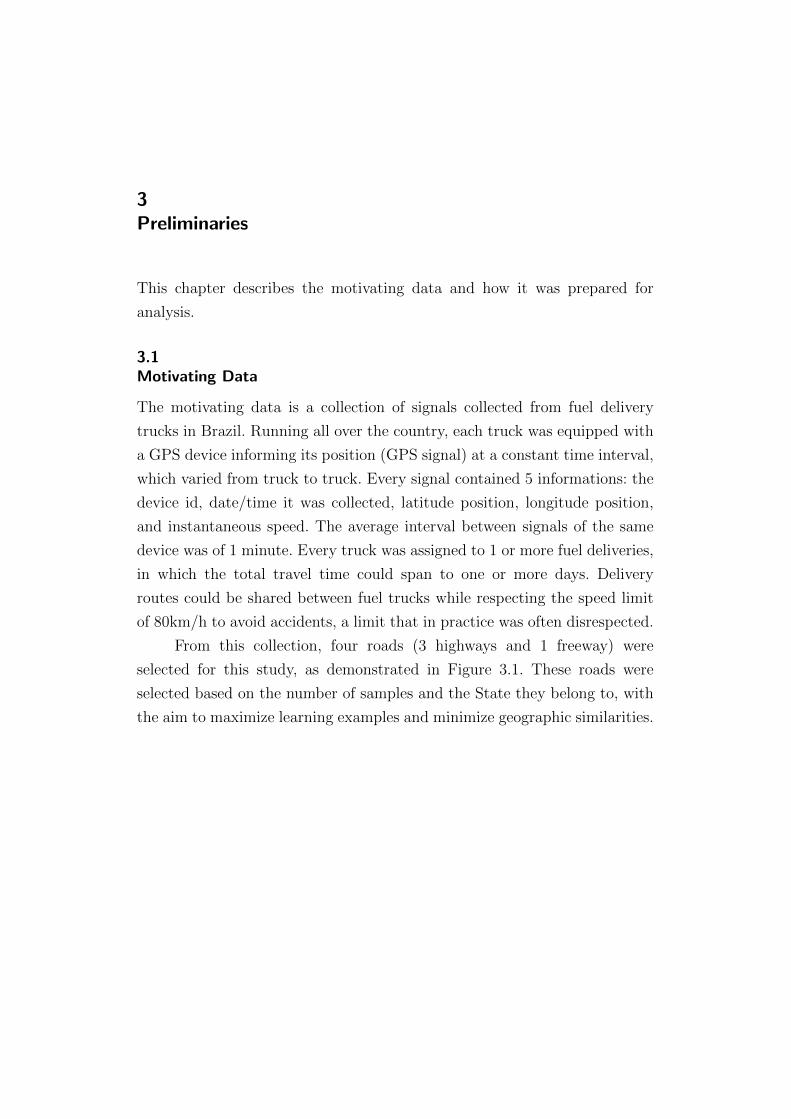
The motivating data is a collection of signals collected from fuel delivery
trucks in Brazil. Running all over the country, each truck was equipped with
a GPS device informing its position (GPS signal) at a constant time interval,
which varied from truck to truck. Every signal contained 5 informations: the
device id, date/time it was collected, latitude position, longitude position,
and instantaneous speed. The average interval between signals of the same
device was of 1 minute. Every truck was assigned to 1 or more fuel deliveries,
in which the total travel time could span to one or more days. Delivery
routes could be shared between fuel trucks while respecting the speed limit
of 80km/h to avoid accidents, a limit that in practice was often disrespected.
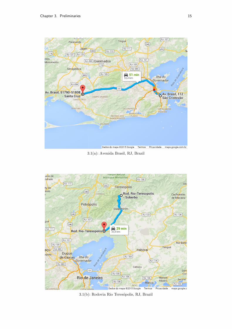
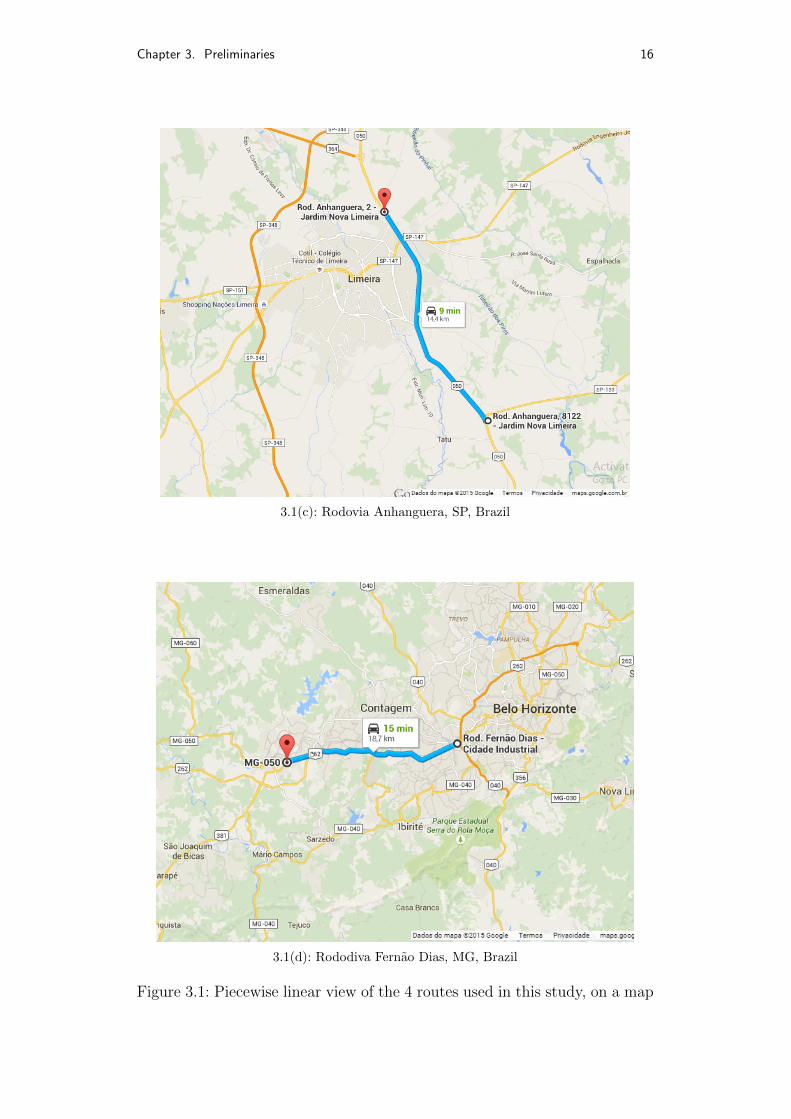
From this collection, four roads (3 highways and 1 freeway) were
selected for this study, as demonstrated in Figure 3.1. These roads were
selected based on the number of samples and the State they belong to, with
the aim to maximize learning examples and minimize geographic similarities.
Chapter 3. Preliminaries 15
3.1(a): Avenida Brasil, RJ, Brazil
3.1(b): Rodovia Rio Teresopolis, RJ, Brazil
Chapter 3. Preliminaries 16
3.1(c): Rodovia Anhanguera, SP, Brazil
3.1(d): Rododiva Fernao Dias, MG, Brazil
Figure 3.1: Piecewise linear view of the 4 routes used in this study, on a map

Chapter 3. Preliminaries 17
3.2Data Preparation
Since the delivery schedule for each truck was unknown, all observations
generated from pair of signals that indicated a speed equal to 0km/h were
ignored. This step was executed because delivery trucks will stop at clients
to deliver its load, and without the truck schedule there is no reliable method
to identify which signal was generated while inside a client, and which signal
was generated while inside a congested road.
3.3Map Matching
In order to identify in which road a given latitude/longitude position may be,
a Map Matching (Brakatsoulas et al., 2005) algorithm should be used. While
many accurate methods (Zheng, 2015) are known to solve this problem, a
simple one was implemented in this study.
Iterating through each road, Map Matching was done in 2 steps: the
first step consisted in projecting the closest point of the current observation
to the current road on the iteration, if closer than a predefined value (ex.
10 meters), it was accepted for that road. The second step was to identify
the direction of each observation by pairing it with the next observation of
the same device. If both occurred inside the signal interval of that device,
they were considered consecutive, and the direction could be determined by
verifying the difference in each signal position.
Prediction accuracy demonstrated to be strongly affected by signal
direction, when direction was not being considered, it dropped to a half or
less than expected.

4Data Analysis
This chapter analyzes the GPS data of each selected road regarding time and
space. Even though mean speed can be related to many factors, these two
properties alone may define accurate patterns for prediction models.
4.1Temporal Analysis
For temporal analysis two visualization types were adopted.
The first visualization type adopted was a heat map of GPS signal
density as a function of hour of day × speed. This visualization type
focuses on assisting temporal pattern identification by evidencing the most
predominant speed value at each hour, and while it may have smaller data
fidelity (when compared to the next visualization type) as a consequence
of smoothing, it certainly makes temporal patterns even more obvious to
spot. Plots generated using this visualization type to compare week days,
as demonstrated in Figure 4.1, indicated that speed behavior on weekends
was different from week days, and that each subset of days must be learned
separately.
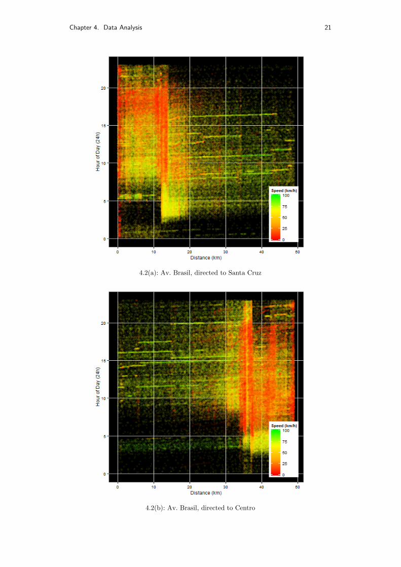
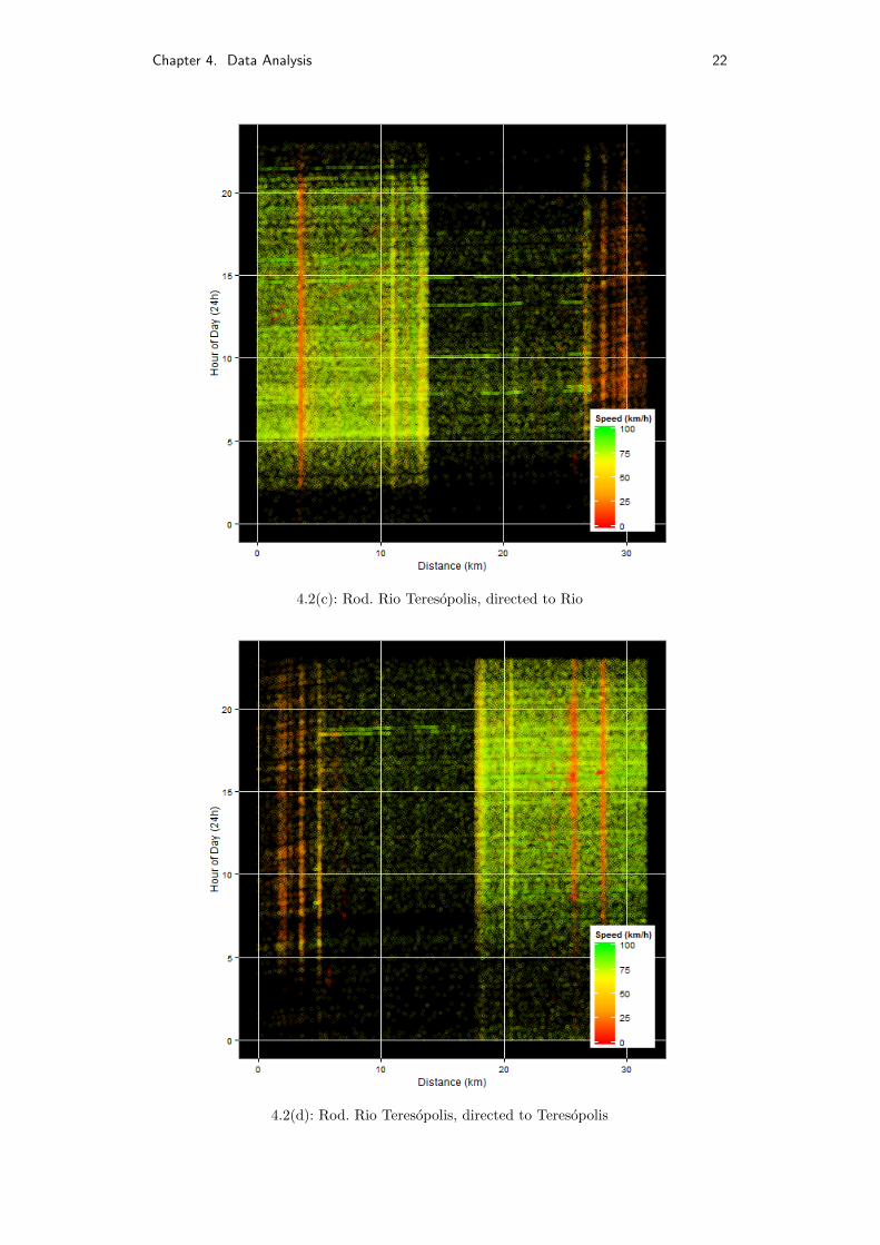
The second visualization type, as demonstrated in Figure 4.2, is a
scatter plot of speed as a function of travel distance × hour of the day, with
an alpha transparency over speed occurrences, using the GPS signal. This
visualization type is focused on data fidelity (no smoothing), while also trying
to assist temporal speed pattern identification. Over the generated plots, a
strong influence of time over speed can be identified quite clearly on Avenida
Brasil and Rodovia Fernao Dias images, while on Rodovia Anhanguera and
Rodovia Rio Teresopolis images the influence of time was much smaller.

Chapter 4. Data Analysis 19
On Avenida Brasil, the first kilometers seem to decrease in speed as time
approaches between 18:00 and 20:00, while on Rodovia Fernao Dias some
kilometers had slower speed concentration at 8:00 to 10:00 and 18:00 to 19:00.
It may be seen as a coincidence, but in Brazil these periods are popularly
known as rush hours, a period of the day in which most workers are going to
and leaving their work place. Figure 4.3 may be used for this purpose also,
but it makes the visual search for this kind of hour pattern less evident.
Overall, these analyses confirmed the existence of sufficient variances
to justify prediction of speed as a function of time, in which time can be
used as a continuous value or a discrete value. In the next section, this study
proposes the use of time as discrete value, with each value representing a
partition of time as hours of a day.

Chapter 4. Data Analysis 20
4.1(a): Saturday 4.1(b): Sunday
4.1(c): Monday 4.1(d): Thursday
4.1(e): Wednesday 4.1(f): Tuesday
4.1(g): Friday
Figure 4.1: GPS signal density plot on Av. Brasil, differentiating weekendsfrom week days
Chapter 4. Data Analysis 21
4.2(a): Av. Brasil, directed to Santa Cruz
4.2(b): Av. Brasil, directed to Centro
Chapter 4. Data Analysis 22
4.2(c): Rod. Rio Teresopolis, directed to Rio
4.2(d): Rod. Rio Teresopolis, directed to Teresopolis

Chapter 4. Data Analysis 23
4.2(e): Rod. Anhanguera, directed to Limeira
4.2(f): Rod. Anhanguera, directed to Americana

Chapter 4. Data Analysis 24
4.2(g): Rod. Fernao Dias, directed to Betim
4.2(h): Rod. Fernao Dias, directed to Belo Horizonte
Figure 4.2: GPS signals observations from the data as a function of space,time, and speed
Chapter 4. Data Analysis 25
4.2Spatial Analysis
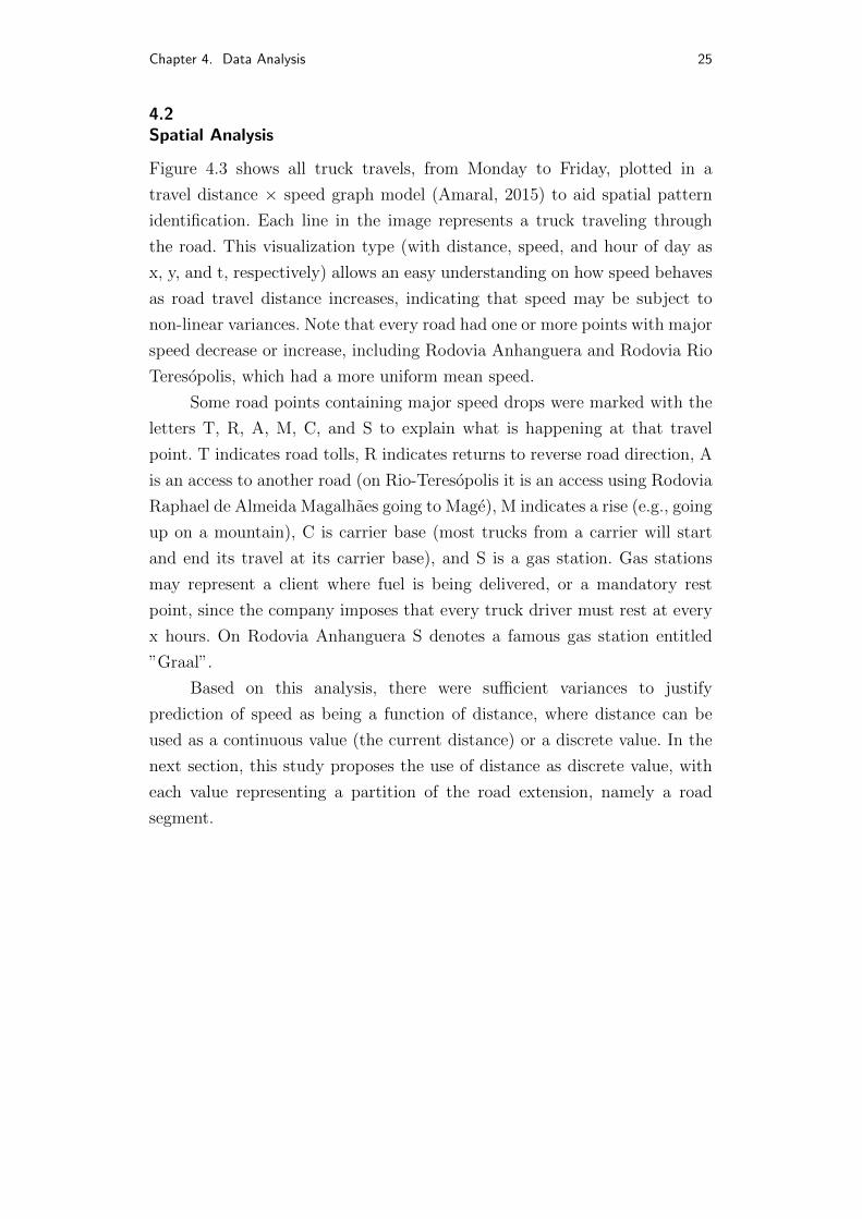
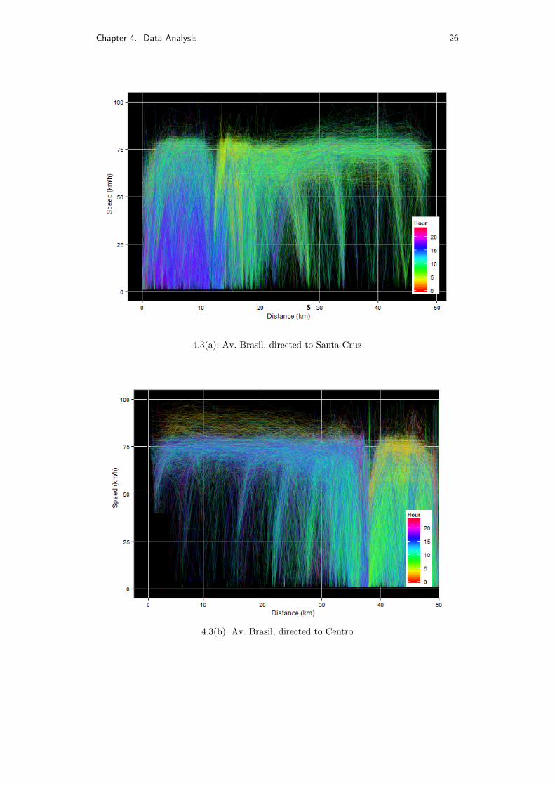
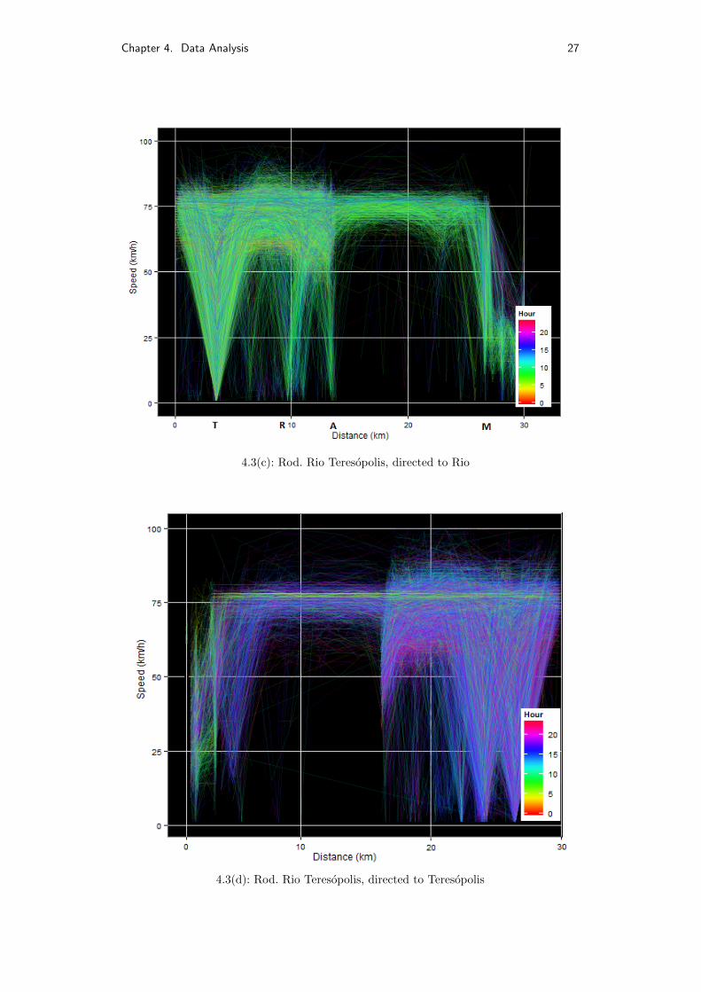
Figure 4.3 shows all truck travels, from Monday to Friday, plotted in a
travel distance × speed graph model (Amaral, 2015) to aid spatial pattern
identification. Each line in the image represents a truck traveling through
the road. This visualization type (with distance, speed, and hour of day as
x, y, and t, respectively) allows an easy understanding on how speed behaves
as road travel distance increases, indicating that speed may be subject to
non-linear variances. Note that every road had one or more points with major
speed decrease or increase, including Rodovia Anhanguera and Rodovia Rio
Teresopolis, which had a more uniform mean speed.
Some road points containing major speed drops were marked with the
letters T, R, A, M, C, and S to explain what is happening at that travel
point. T indicates road tolls, R indicates returns to reverse road direction, A
is an access to another road (on Rio-Teresopolis it is an access using Rodovia
Raphael de Almeida Magalhaes going to Mage), M indicates a rise (e.g., going
up on a mountain), C is carrier base (most trucks from a carrier will start
and end its travel at its carrier base), and S is a gas station. Gas stations
may represent a client where fuel is being delivered, or a mandatory rest
point, since the company imposes that every truck driver must rest at every
x hours. On Rodovia Anhanguera S denotes a famous gas station entitled
”Graal”.
Based on this analysis, there were sufficient variances to justify
prediction of speed as being a function of distance, where distance can be
used as a continuous value (the current distance) or a discrete value. In the
next section, this study proposes the use of distance as discrete value, with
each value representing a partition of the road extension, namely a road
segment.
Chapter 4. Data Analysis 26
4.3(a): Av. Brasil, directed to Santa Cruz
4.3(b): Av. Brasil, directed to Centro
Chapter 4. Data Analysis 27
4.3(c): Rod. Rio Teresopolis, directed to Rio
4.3(d): Rod. Rio Teresopolis, directed to Teresopolis
Chapter 4. Data Analysis 28
4.3(e): Rod. Anhanguera, directed to Limeira
4.3(f): Rod. Anhanguera, directed to Americana

Chapter 4. Data Analysis 29
4.3(g): Rod. Fernao Dias, directed to Betim
4.3(h): Rod. Fernao Dias, directed to Belo Horizonte
Figure 4.3: Travel plot obtained from the data as a function of space, speedand time

5Spatio-Temporal Partitioning
This chapter proposes a spatial-temporal partition strategy based on the
previously discussed spatio-temporal analysis. Although there are many
different ways to proceed, this work selected an heuristic based on the
statistics of the historic GPS data.
5.1Spatial Partitioning
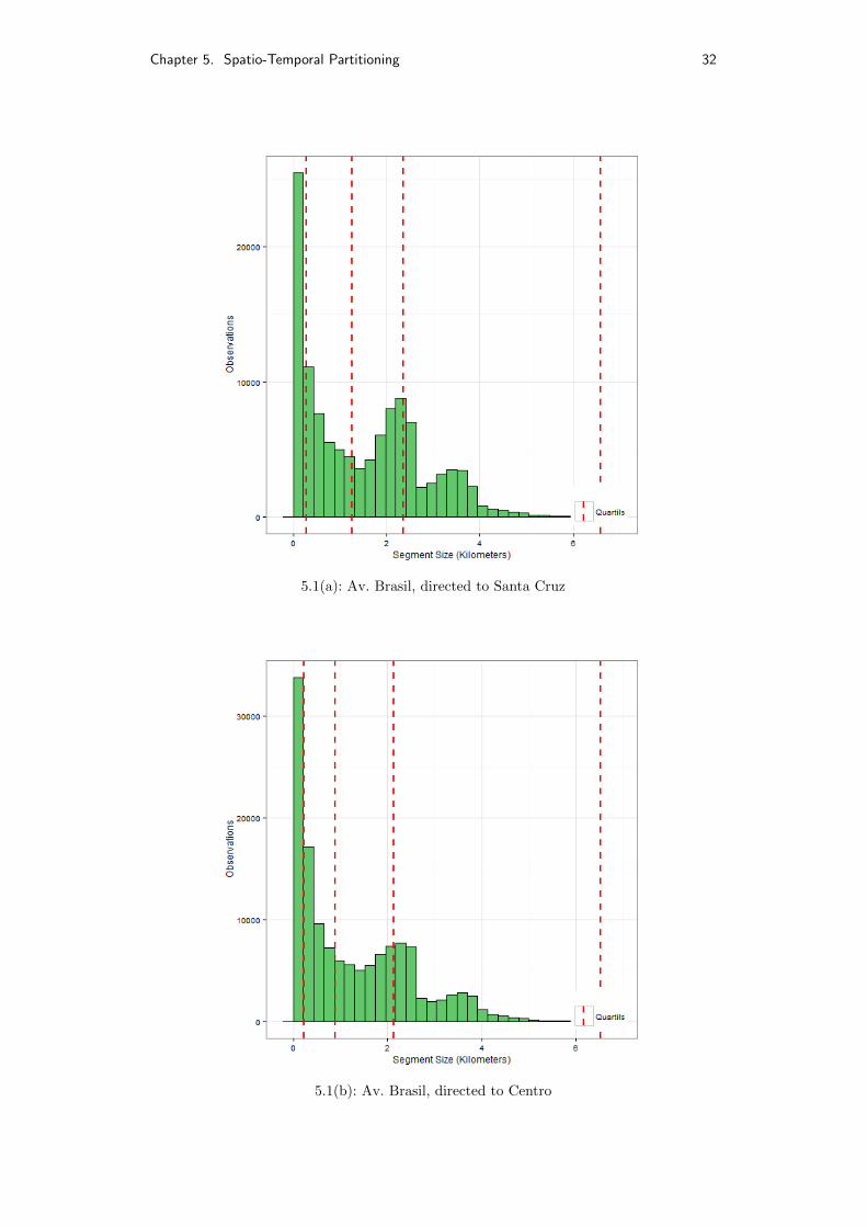
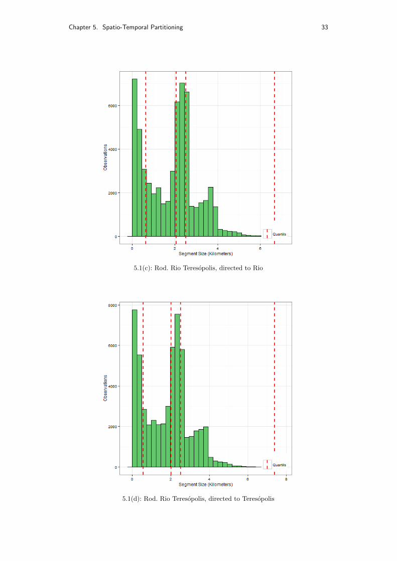
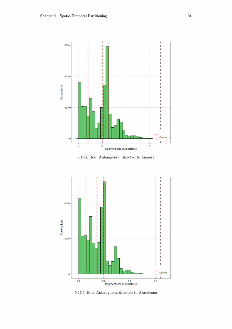
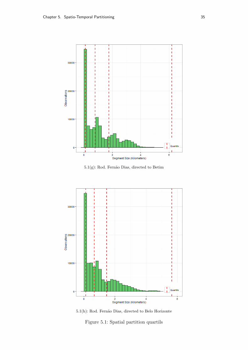
Supported by the previous spatial analysis, this study proposes
partitioning a road extension into segments, where the segment size is selected
based on the average distance traveled between each pair of consecutive
signals of the same vehicle. The objective is to find the segment size that
best learns from the given gps road observations.
In order to visualize the distance distribution over these pairs, a
histogram was generated, as illustrated in Figure 5.1, indicating that each
road should have its own segment size. The proposal is to use the median
value as the segment size, since it is simple to calculate and should perform
reasonably in most cases, but it is important to note that, although it is a
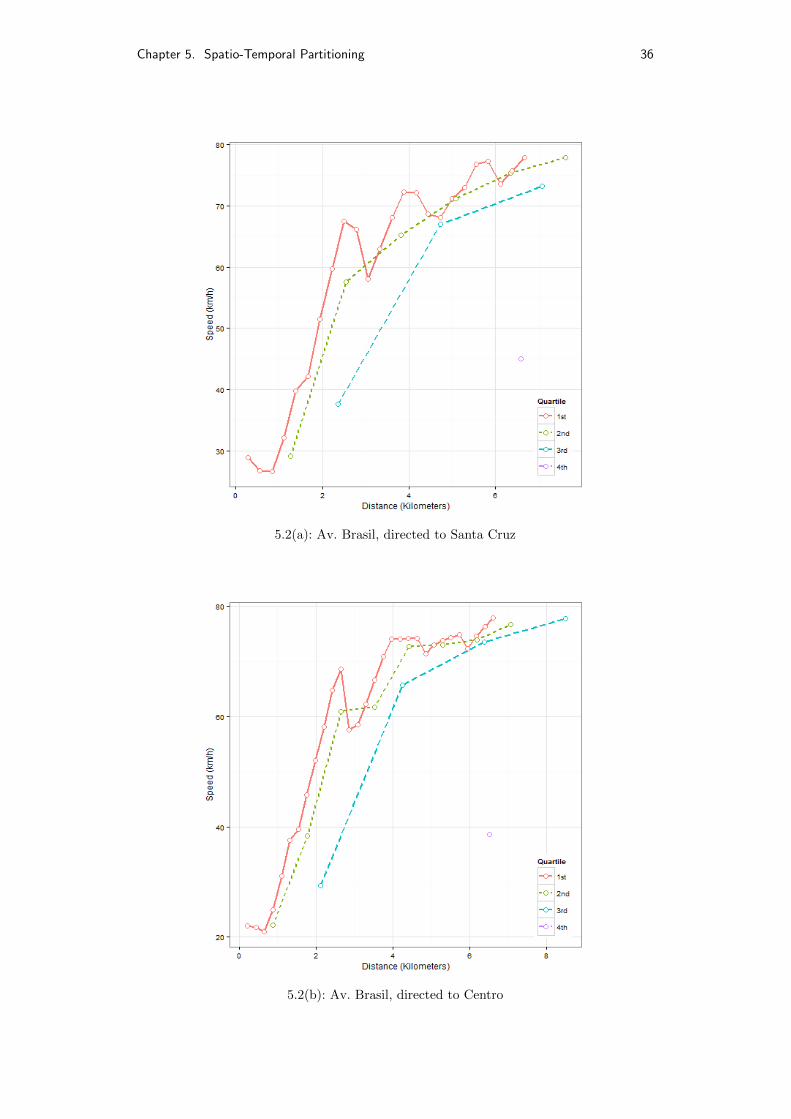
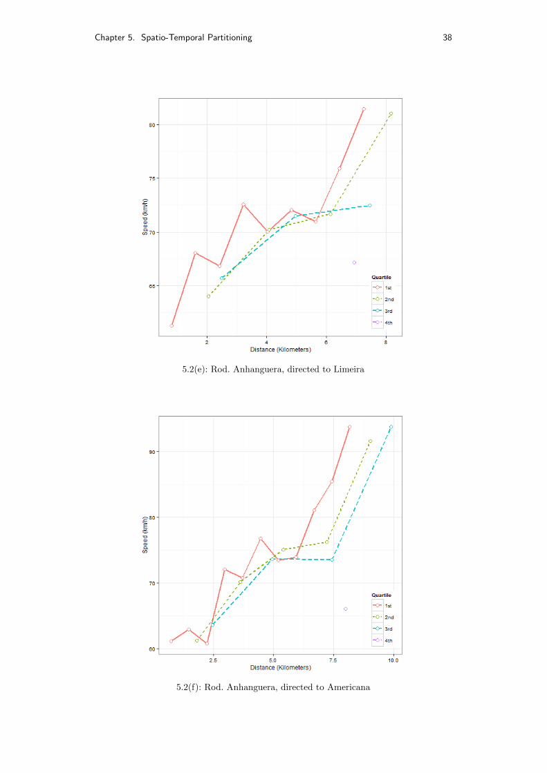
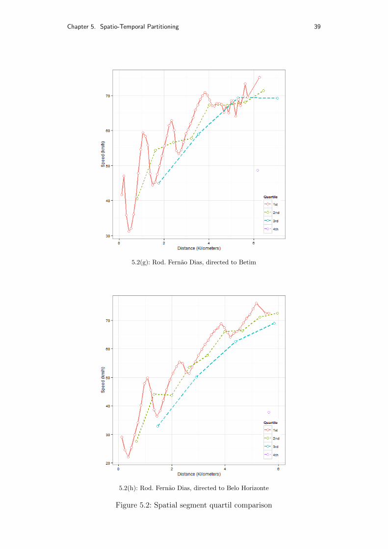
good choice, the median is not necessarily optimum. Quartile analysis of these
same distances, as shown in Figure 5.2, demonstrated that smaller segment
sizes should give even more information about the average speed, while large
sizes will tend to over generalize it. Mean speed was over generalized as the
segment was over sized (3rd and 4th quartiles), and although the 1st quartile
appeared to be an even better choice than the 2nd quartile, in some cases,
the “shorter is better” approach won’t always give the best prediction if
the selected size is too small. If a 1 meter sized is used, there may be no

Chapter 5. Spatio-Temporal Partitioning 31
improvement in prediction accuracy, and if the data doesn’t provide a good
amount of observations for every 1 meter on the road, it will add unnecessary
complexity to the model, making the learning process slower.
Chapter 5. Spatio-Temporal Partitioning 32
5.1(a): Av. Brasil, directed to Santa Cruz
5.1(b): Av. Brasil, directed to Centro
Chapter 5. Spatio-Temporal Partitioning 33
5.1(c): Rod. Rio Teresopolis, directed to Rio
5.1(d): Rod. Rio Teresopolis, directed to Teresopolis
Chapter 5. Spatio-Temporal Partitioning 34
5.1(e): Rod. Anhanguera, directed to Limeira
5.1(f): Rod. Anhanguera, directed to Americana
Chapter 5. Spatio-Temporal Partitioning 35
5.1(g): Rod. Fernao Dias, directed to Betim
5.1(h): Rod. Fernao Dias, directed to Belo Horizonte
Figure 5.1: Spatial partition quartils
Chapter 5. Spatio-Temporal Partitioning 36
5.2(a): Av. Brasil, directed to Santa Cruz
5.2(b): Av. Brasil, directed to Centro

Chapter 5. Spatio-Temporal Partitioning 37
5.2(c): Rod. Rio Teresopolis, directed to Rio
5.2(d): Rod. Rio Teresopolis, directed to Teresopolis
Chapter 5. Spatio-Temporal Partitioning 38
5.2(e): Rod. Anhanguera, directed to Limeira
5.2(f): Rod. Anhanguera, directed to Americana
Chapter 5. Spatio-Temporal Partitioning 39
5.2(g): Rod. Fernao Dias, directed to Betim
5.2(h): Rod. Fernao Dias, directed to Belo Horizonte
Figure 5.2: Spatial segment quartil comparison
Chapter 5. Spatio-Temporal Partitioning 40
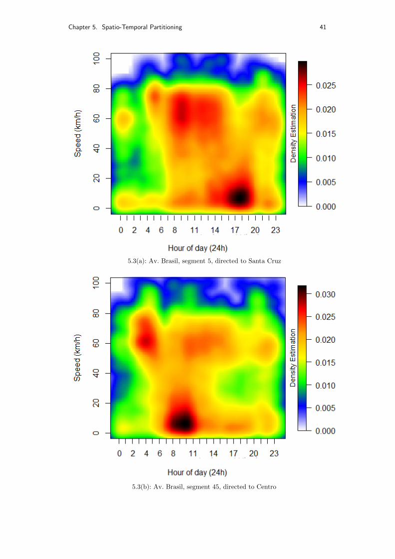
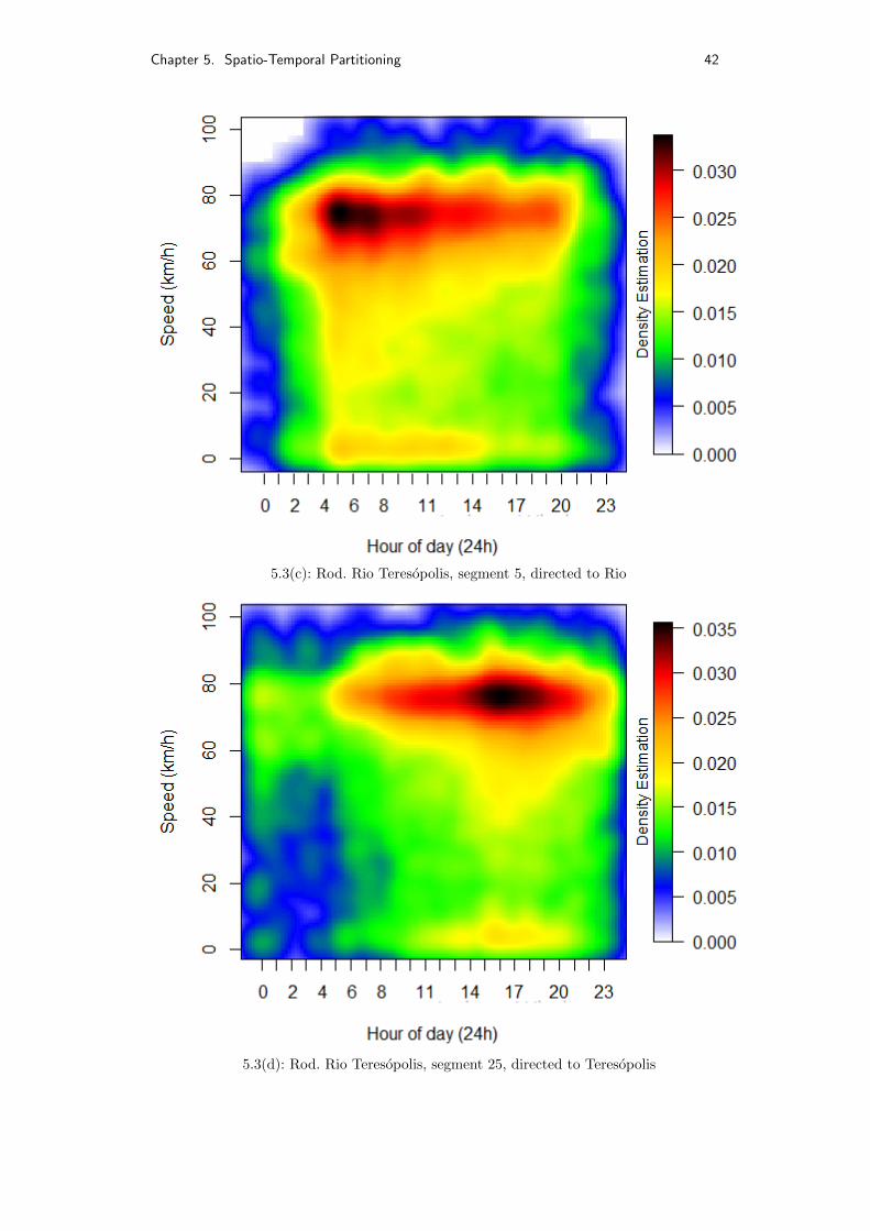
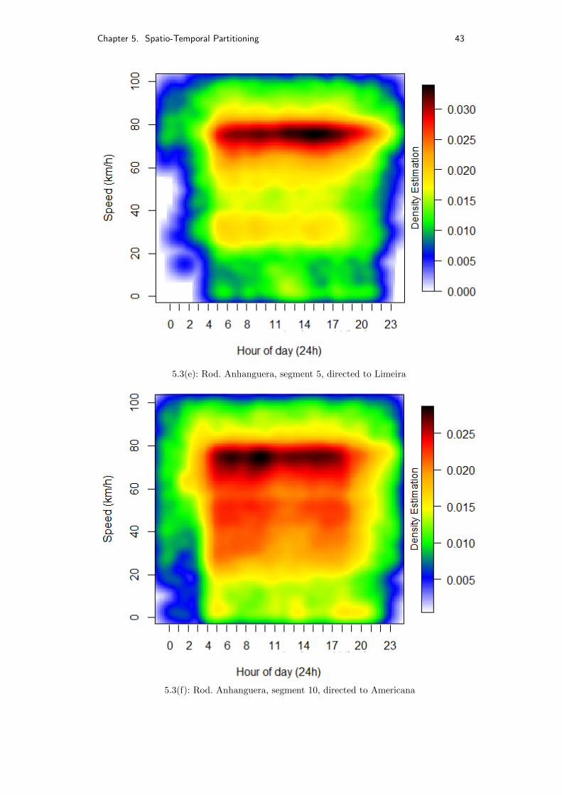
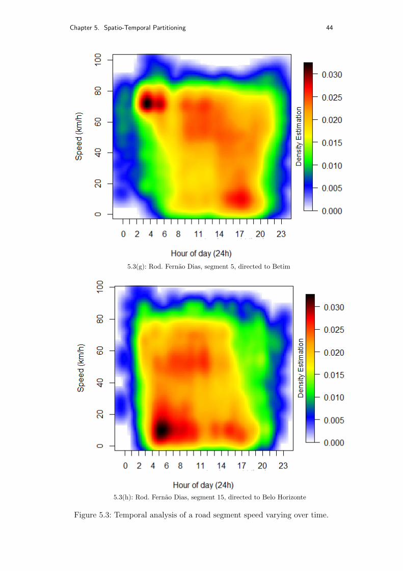
5.2Temporal Partitioning
For temporal partition, this study proposes a time segmentation into hours.
This choice was based mostly on the number of observations and prediction
relevance.
Since a spatial partitioning was applied as well, a segment from each
road was selected and studied in both directions with an hourly partition.
Using a density plot with speed as a function of time, as shown in Figure 5.3,
speed patterns could be identified at each road. While different speeds can be
observed at the same hour, it is clear that each hour has a higher density at a
determined speed value, and that each hour has its own average speed. These
behaviors were especially evident on Avenida Brasil and Rodovia Fernao
Dias.
A curious pattern on Avenida Brasil was that, when directed to Rio,
speed decreases from 8:00 to 11:00. On the other hand, it increases in the
afternoon and decreases again from 17:00 to 20:00, when directed to Santa
Cruz. It may be seen as a coincidence again, but there is high traffic going to
Rio in the morning followed by high traffic leaving Rio at night, very similar
to a Rush Hour in Brazil.
Chapter 5. Spatio-Temporal Partitioning 41
5.3(a): Av. Brasil, segment 5, directed to Santa Cruz
5.3(b): Av. Brasil, segment 45, directed to Centro
Chapter 5. Spatio-Temporal Partitioning 42
5.3(c): Rod. Rio Teresopolis, segment 5, directed to Rio
5.3(d): Rod. Rio Teresopolis, segment 25, directed to Teresopolis
Chapter 5. Spatio-Temporal Partitioning 43
5.3(e): Rod. Anhanguera, segment 5, directed to Limeira
5.3(f): Rod. Anhanguera, segment 10, directed to Americana
Chapter 5. Spatio-Temporal Partitioning 44
5.3(g): Rod. Fernao Dias, segment 5, directed to Betim
5.3(h): Rod. Fernao Dias, segment 15, directed to Belo Horizonte
Figure 5.3: Temporal analysis of a road segment speed varying over time.

Chapter 5. Spatio-Temporal Partitioning 45
5.3Proposed Solution
The proposed solution is a model based on the described spatio-temporal
partitions to obtain mean speed predictions of a road. This model will predict
the mean speed for a given road segment at a given hour of the day. The
main idea is to group speed observations by two factors: the segment where
it occurred, and the hour of the day when it was observed. To distinguish it
from other models the word ”STM” (Spatio-Temporal Model) will be used
to reference it.
5.3.1Concept
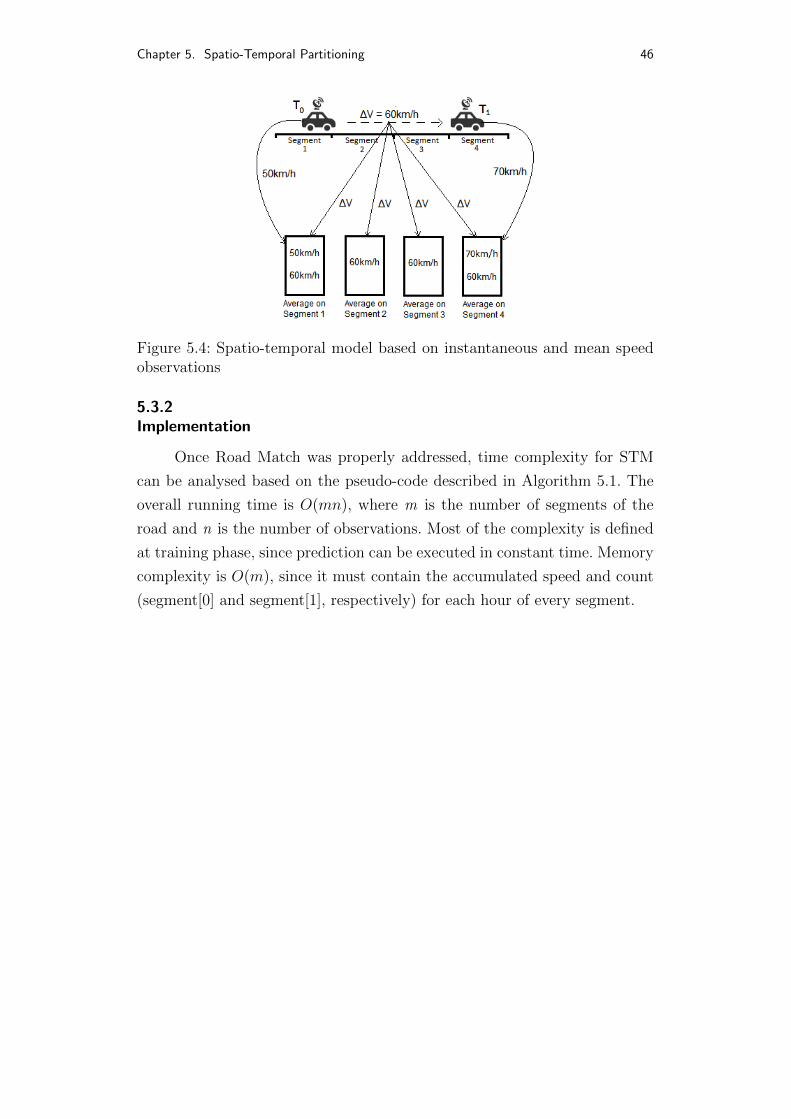
STM construction can be divided in 3 steps. The first step consists in
calculating the mean speed observed from each pair of consecutive signals of
the same vehicle, in order to use them as speed observations on each road
segment the underlying pair travelled through. The second step is to add the
instantaneous speed provided with the GPS signal in the exact road segment
it was collected. Figure 5.4 visually illustrates procedures for both steps 1
and 2. The third and final step is to group speeds at each segment by the
hour of the day that they were observed, meaning that each segment will be
divided into 24 subgroups (24 hours), in which each subgroup will contain
the average of all speed observations occurred in that segment at that hour.
Accurate Instantaneous GPS Speeds are usually calculated using
Doppler Shifts (Townshend et al., 2008) and will only be available if the GPS
device supports this functionality. When unavailable, the second step of the
building procedure can be ignored in favour of a model variation using only
the calculated mean speeds from each consecutive pair of the same vehicle.
Prediction performance from both STM variations, using only instantaneous
speeds and using only calculated mean speeds, were compared with STM
(which uses both instantaneous and mean speeds) indicating that, while STM
was superior in overall, MAE results varied at a maximum of 10% from its
variations.
Chapter 5. Spatio-Temporal Partitioning 46
Figure 5.4: Spatio-temporal model based on instantaneous and mean speedobservations
5.3.2Implementation
Once Road Match was properly addressed, time complexity for STM
can be analysed based on the pseudo-code described in Algorithm 5.1. The
overall running time is O(mn), where m is the number of segments of the
road and n is the number of observations. Most of the complexity is defined
at training phase, since prediction can be executed in constant time. Memory
complexity is O(m), since it must contain the accumulated speed and count
(segment[0] and segment[1], respectively) for each hour of every segment.

Chapter 5. Spatio-Temporal Partitioning 47
Algorithm 5.1 Spatio-temporal prediction model
1: function LEARN(signalPairs, segments)2: for pair in signalPairs do3: hour ← pair.hour4: start← pair.start5: end← pair.end6: mean← (end.distance− start.distance)/pair.elapsed7: for segmentIndex in pair.travelledSegments do8: segments[segmentIndex][hour][0] =+ mean9: segments[segmentIndex][hour][1] =+ 1
10: end for11: segments[start.segmentIndex][hour][0] += start.instantSpeed12: segments[start.segmentIndex][hour][1] += 113: segments[end.segmentIndex][hour][0] += end.instantSpeed14: segments[end.segmentIndex][hour][1] += 115: end for16: end function17: function PREDICT(segmentIndex, hour, segments)18: accumulatedSpeed = segments[segmentIndex][hour][0]19: observationCount = segments[segmentIndex][hour][1]20: return accumulatedSpeed/observationCount21: end function
6Experiments
Prediction experiments were carried out using 10 million signals from 10
thousand distinct fuel trucks in raw GPS format. This data contains all
signals generated during the year of 2013, along with signals from the first two
months of 2014, in four different roads: Avenida Brasil, Rodovia Anhanguera,
Rodovia Rio Teresopolis and Rodovia Fernao Dias, as previously mentioned.
6.1Experimental Setup
Data was sorted by date in ascending order and then divided into 3 different
subsets: training, validation and test. The date sort is important in order
to assure that prediction is based only on historic observations, excluding
current and future ones while the subsets training, validation, and test
sets, with sizes 64%, 16%, 20%, respectively, are a commonly used learning
strategy to avoid over-fitting. Using this methodology, subsets training and
validation contained only data from 2013, while the test subset contained
only data from 2014.
6.2Evaluation Measures
Four measures were used to compare the results of the methods: RMSE,
MAE, MAD, and MAPE.
Root Mean Squared Error (RMSE) is one of the most commonly used
metrics for regression models, it represents the prediction error standard
deviation and is defined as:√
1n
∑ni=1(Yi − Yi)2.
Chapter 6. Experiments 49
Mean Absolute Error (MAE) is also a commonly used metric for
regression and is being adopted as the reference metric in this study in favor
of RMSE. It is less influenced by outliers and thus closer to what this study
tries to measure. MAE is defined as follows: 1n
∑ni=1 |Yi − Yi|.
Median Absolute Deviation (MAD) is a statistically robust measure of
the prediction error variability and is defined as: median(|Yi−median(|Yj −Yj|)|).
Mean Absolute Percentage Error (MAPE) is another commonly used
metric for regression models. It measures prediction accuracy as a percentage
value indicating how much of an observation can be predicted, in average,
using the specified model. MAPE is defined as follows: 1n
∑ni=1 |
Yi−Yi
Yi|.
6.3Implemented Methods
To understand the performance of STM an instantaneous speed prediction
experiment was proposed using five methods. Method 1 uses the road mean
speed as the predicted speed. Method 2 calculates a mean speed for each
road segment and uses the mean speed at the segment where the sample
was collected as the predicted speed. Method 3 calculates a mean speed for
each hour of the day and uses the mean speed at the hour that sample
was collected as the predicted speed. Method 4 represents the baseline, using
Support Vector Regression on 2 features: distance (from road start) and hour
of the day to predict the speed. Method 5 uses the STM model proposed in
this study, which predicts speed based on a road segment and hour of the
day.
6.4Experimental Results
Using the implemented methods, an instantaneous speed prediction
experiment was then conducted. Tables 6.1, 6.2, and 6.3 demonstrate
prediction results using the metrics MAE, RMSE, and MAD, respectively.
Comparing results from MAE, Method 1 was expected to have the worst
performance between the implemented methods, but method 4 scored worse
Chapter 6. Experiments 50
on Rodovia Fernao Dias. Method 2 consistently outperformed methods 1,
3, and 4 on every road, indicating that spatial partitions are relevant for
prediction, even more relevant than temporal partitions (using hours). It
improved prediction error up to 40% when compared to method 4, and up
to 50% when compared to method 1, while also being the best method in
one direction of Rodovia Rio Teresopolis. While not as relevant as method
2, method 3 performed, most of the time, better than or near Method 1,
indicating that in some roads time partitions will also improve prediction up
10% when compared to method 1. Method 4, the baseline, performed better
on the roads Rodovia Anhanguera and Rodovia Rio Teresopolis, where speed
was more uniform along the road extension, on the other roads, however, it
failed to improve prediction, even when compared to method 1 that applied
a naive mean. Method 5 (STM) outperformed all of the other implemented
methods, with the exception of a direction on Rodovia Rio Teresopolis, and
close to the best result on the worst case, indicating that the union of space
and time can improve prediction even further than using each dimension
separately. STM improved prediction up to 55% when compared to method
1, 40% when compared to method 2, 55% when compared to method 3, and
50% when compared to method 4.
Running times for both methods 4 and 5 are presented in Table 6.4,
method 5 was up to seven times faster than method 4, using LIBLINEAR
(Fan et al., 2008), the fastest SVR implementation available at the time of
writing.
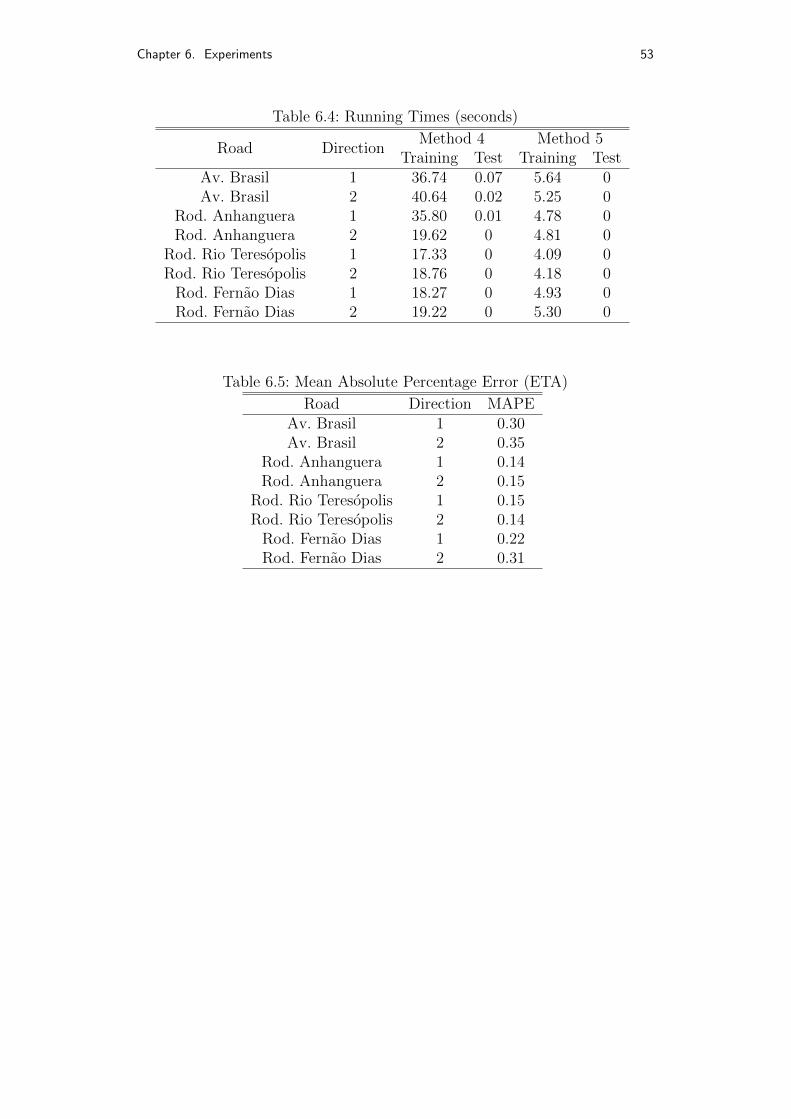
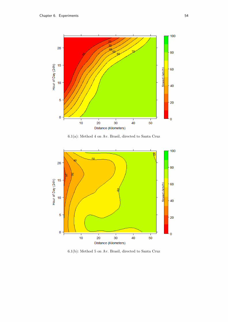
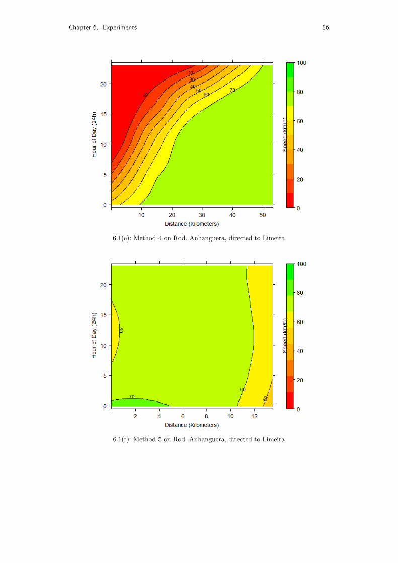
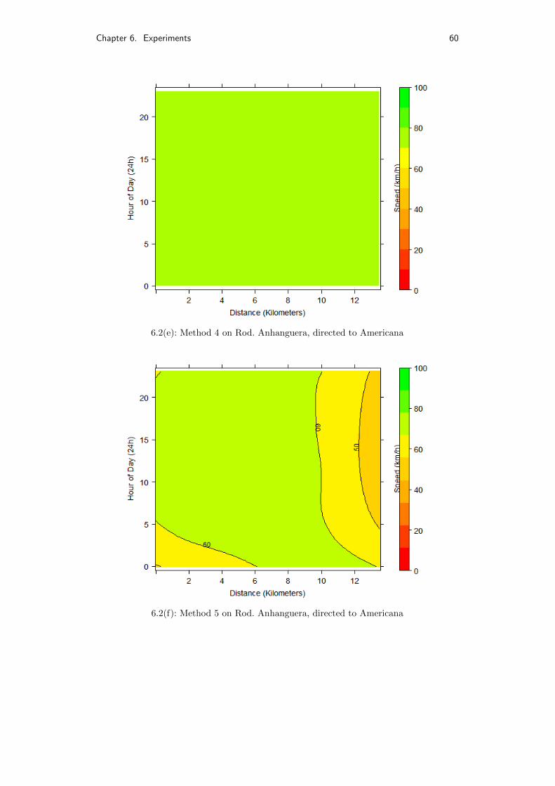
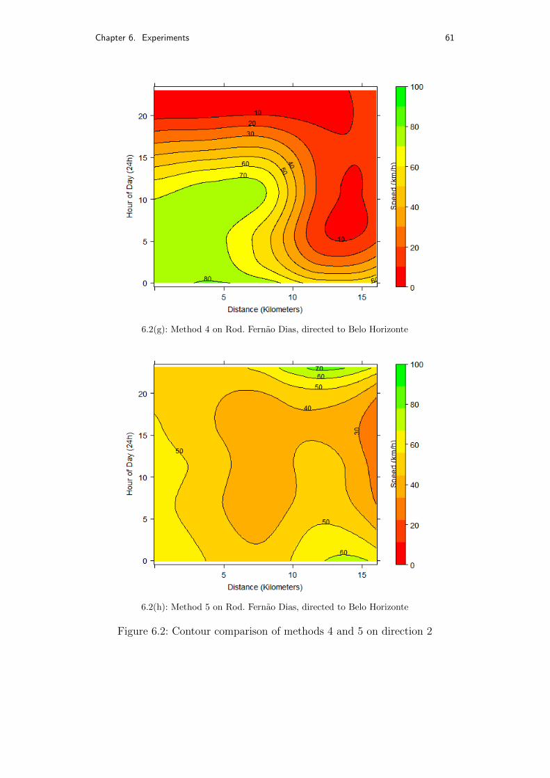
Comparing STM with its baseline, Figures 6.1 and 6.2 show a heat map
representing the estimated velocity from methods 4 and 5, for each road in
each direction. Contour lines were added to delimite speed regions relative
to both time and space dimensions. The number of regions identified using
method 5 were considerably greater than the ones identified with method 4
(SVR). Visually, method 4 demonstrated difficulty at identifying suddenly
decreases or increases in speed when compared to method 5 (STM), a
deficiency that may render it inferior at identifying either spatial or temporal
patterns, possibly justifying why method 5 achieved superior prediction
results. While method 5 had middle regions shifting speed, method 4 appears
Chapter 6. Experiments 51
to choose a direction to always increase or decrease it in a generalized smooth
behaviour, as if speed could not change drastically in the middle of the road,
or the day, and get back to the average speed again in later observations.
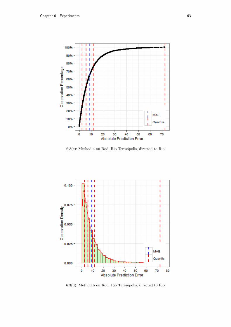
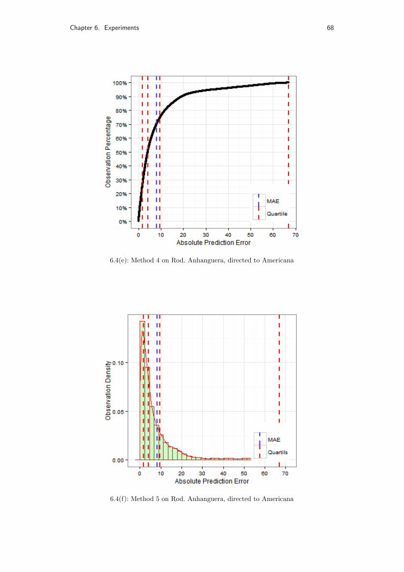
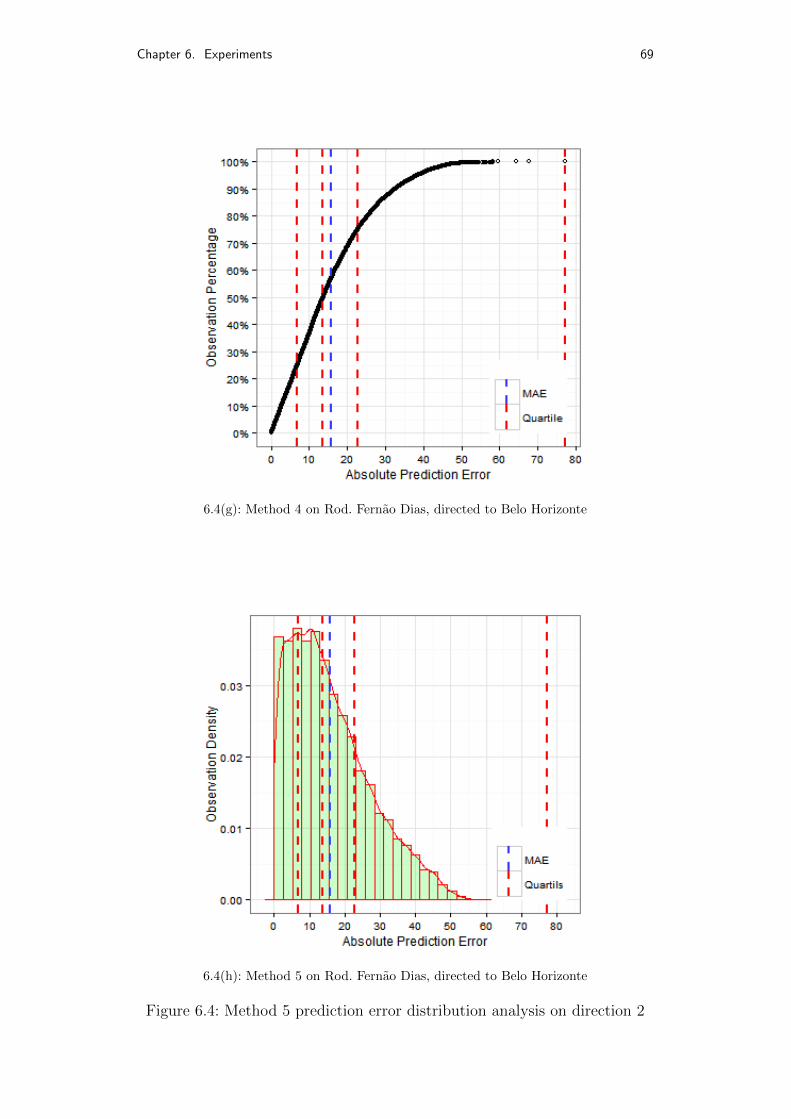
Performance from method 5 can be further analyzed in Figures 6.3 and
6.4. For each road, two plots were generated: one to demonstrate the absolute
error growth over the observation population, and another to demonstrate
the absolute error distribution. The first plot was used to visualize the curve
slope as the absolute error grows, and results indicated that 60% to 70%
of the observations had an error lesser than or equal to the MAE. The
second plot was important to give another view of the results, having higher
concentrations on lower values, and smaller concentration on higher values
is an indication that STM is performing accordingly.
A last experiment was conducted to predict ETA. While instantaneous
speed prediction refers to a single moment of a vehicle during its travel
on a road, ETA refers to its whole passage, which constitutes a set of
moments where a faulty prediction at a single segment may not influence
travel prediction as a whole. ETA can be predicted for a pair of consecutive
signals of the same device by dividing the distance it travelled through on
each segment by the predicted mean speed of that segment at that same
hour. As defined by the equation:
( ˆY1,j ×D1) + (n−1∑i=2
s
Yi,j
) + ( ˆYn,j ×Dn−1)
Where n is the number of segments the pair travelled through, s is the
size of a segment in kilometres, Yi,j is the predicted mean speed of travelled
segments set on index i at hour j, and Di is the distance travelled on travelled
segments set at index i. 6.5 presents results of the ETA experiment. Near state
of the art results were achieved in Rodovia Rio teresopolis (14% and 16%
of error) and Rodovia Anhanguera (16% and 17% of error), while Avenida
Brasil and Fernao Dias proved to be challenger. These results are impressive
considering that no real time data was used, and that predictions ranged
from 1 to 2 months ahead of the training data, contrary to the current state
of the art models, which require real time data and are focused on short-time
Chapter 6. Experiments 52
predictions.
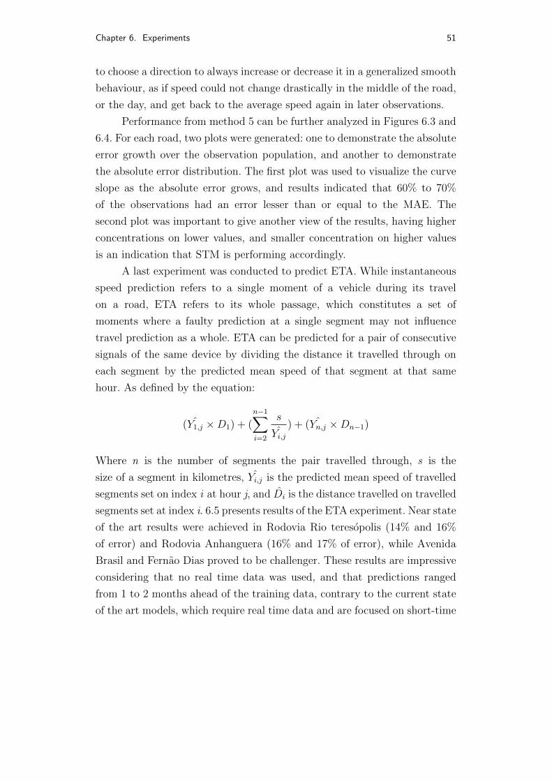
Table 6.1: Mean Absolute Error (km/h)
Road DirectionMethod
1 2 3 4 5Av. Brasil 1 25.52 20.26 23.78 24.03 11.96Av. Brasil 2 25.78 19.98 25.19 22.59 13.92
Rod. Anhanguera 1 12.48 10.40 12.46 11.02 8.33Rod. Anhanguera 2 13.45 9.97 13.47 11.95 8.15
Rod. Rio Teresopolis 1 15.14 7.99 15.09 9.85 6.96Rod. Rio Teresopolis 2 14.64 9.23 14.57 12.84 9.42
Rod. Fernao Dias 1 22.65 20.97 20.48 28.69 15.61Rod. Fernao Dias 2 20.61 17.19 19.99 28.28 15.83
Table 6.2: Root Mean Squared Error (km/h)
Road DirectionMethod
1 2 3 4 5Av. Brasil 1 28.45 23.30 28.00 33.32 16.17Av. Brasil 2 27.98 23.09 28.37 32.47 17.89
Rod. Anhanguera 1 17.89 15.91 17.89 20.18 14.15Rod. Anhanguera 2 18.50 15.65 18.51 20.68 13.85
Rod. Rio Teresopolis 1 19.21 12.42 19.14 17.45 10.88Rod. Rio Teresopolis 2 18.82 13.04 18.76 20.67 13.44
Rod. Fernao Dias 1 25.84 25.52 24.05 37.18 19.62Rod. Fernao Dias 2 23.29 21.21 22.81 35.48 19.48
Table 6.3: Median Absolute Deviation (km/h)
Road DirectionMethod
1 2 3 4 5Av. Brasil 1 10.00 8.32 11.39 13.00 5.72Av. Brasil 2 7.14 8.41 9.46 10.00 6.91
Rod. Anhanguera 1 3.00 4.15 3.43 3.00 3.09Rod. Anhanguera 2 4.00 4.19 4.64 3.00 3.23
Rod. Rio Teresopolis 1 4.67 3.38 3.68 4.00 3.27Rod. Rio Teresopolis 2 5.00 4.37 5.07 5.00 4.36
Rod. Fernao Dias 1 9.08 10.47 9.76 20.00 8.10Rod. Fernao Dias 2 9.00 8.63 8.87 19.00 7.88
Chapter 6. Experiments 53
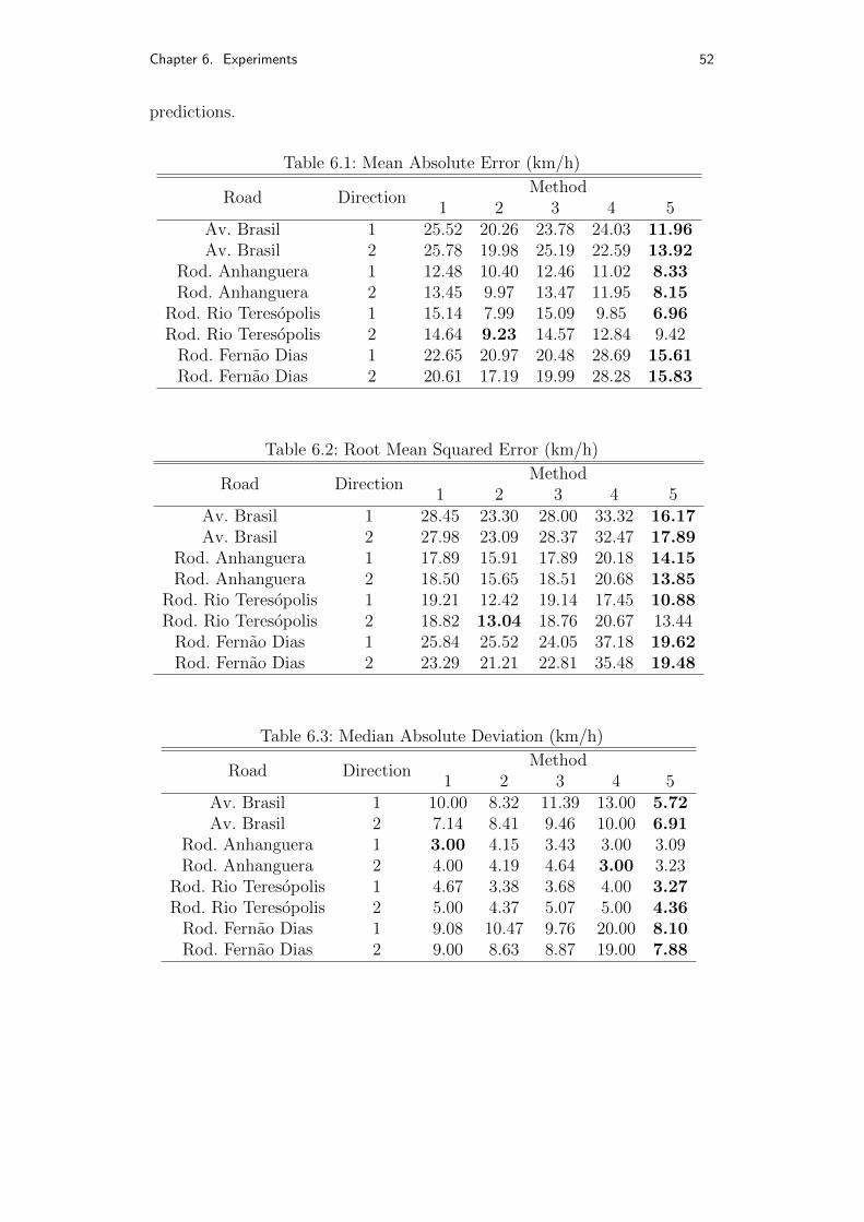
Table 6.4: Running Times (seconds)
Road DirectionMethod 4 Method 5
Training Test Training TestAv. Brasil 1 36.74 0.07 5.64 0Av. Brasil 2 40.64 0.02 5.25 0
Rod. Anhanguera 1 35.80 0.01 4.78 0Rod. Anhanguera 2 19.62 0 4.81 0
Rod. Rio Teresopolis 1 17.33 0 4.09 0Rod. Rio Teresopolis 2 18.76 0 4.18 0
Rod. Fernao Dias 1 18.27 0 4.93 0Rod. Fernao Dias 2 19.22 0 5.30 0
Table 6.5: Mean Absolute Percentage Error (ETA)
Road Direction MAPEAv. Brasil 1 0.30Av. Brasil 2 0.35
Rod. Anhanguera 1 0.14Rod. Anhanguera 2 0.15
Rod. Rio Teresopolis 1 0.15Rod. Rio Teresopolis 2 0.14
Rod. Fernao Dias 1 0.22Rod. Fernao Dias 2 0.31
Chapter 6. Experiments 54
6.1(a): Method 4 on Av. Brasil, directed to Santa Cruz
6.1(b): Method 5 on Av. Brasil, directed to Santa Cruz

Chapter 6. Experiments 55
6.1(c): Method 4 on Rod. Rio Teresopolis, directed to Rio
6.1(d): Method 5 on Rod. Rio Teresopolis, directed to Rio
Chapter 6. Experiments 56
6.1(e): Method 4 on Rod. Anhanguera, directed to Limeira
6.1(f): Method 5 on Rod. Anhanguera, directed to Limeira

Chapter 6. Experiments 57
6.1(g): Method 4 on Rod. Fernao Dias, directed to Betim
6.1(h): Method 5 on Rod. Fernao Dias, directed to Betim
Figure 6.1: Contour comparison of methods 4 and 5 on direction 1

Chapter 6. Experiments 58
6.2(a): Method 4 on Av. Brasil, directed to Centro
6.2(b): Method 5 on Av. Brasil, directed to Centro

Chapter 6. Experiments 59
6.2(c): Method 4 on Rod. Rio Teresopolis, directed to Teresopolis
6.2(d): Method 5 on Rod. Rio Teresopolis, directed to Teresopolis
Chapter 6. Experiments 60
6.2(e): Method 4 on Rod. Anhanguera, directed to Americana
6.2(f): Method 5 on Rod. Anhanguera, directed to Americana
Chapter 6. Experiments 61
6.2(g): Method 4 on Rod. Fernao Dias, directed to Belo Horizonte
6.2(h): Method 5 on Rod. Fernao Dias, directed to Belo Horizonte
Figure 6.2: Contour comparison of methods 4 and 5 on direction 2

Chapter 6. Experiments 62
6.3(a): Method 4 on Av. Brasil, directed to Santa Cruz
6.3(b): Method 5 on Av. Brasil, directed to Santa Cruz
Chapter 6. Experiments 63
6.3(c): Method 4 on Rod. Rio Teresopolis, directed to Rio
6.3(d): Method 5 on Rod. Rio Teresopolis, directed to Rio

Chapter 6. Experiments 64
6.3(e): Method 4 on Rod. Anhanguera, directed to Limeira
6.3(f): Method 5 on Rod. Anhanguera, directed to Limeira

Chapter 6. Experiments 65
6.3(g): Method 4 on Rod. Fernao Dias, directed to Betim
6.3(h): Method 5 on Rod. Fernao Dias, directed to Betim
Figure 6.3: Method 5 prediction error distribution analysis on direction 1
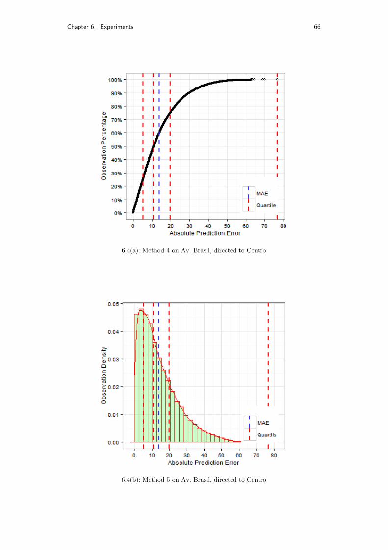
Chapter 6. Experiments 66
6.4(a): Method 4 on Av. Brasil, directed to Centro
6.4(b): Method 5 on Av. Brasil, directed to Centro

Chapter 6. Experiments 67
6.4(c): Method 4 on Rod. Rio Teresopolis, directed to Teresopolis
6.4(d): Method 5 on Rod. Rio Teresopolis, directed to Teresopolis
Chapter 6. Experiments 68
6.4(e): Method 4 on Rod. Anhanguera, directed to Americana
6.4(f): Method 5 on Rod. Anhanguera, directed to Americana
Chapter 6. Experiments 69
6.4(g): Method 4 on Rod. Fernao Dias, directed to Belo Horizonte
6.4(h): Method 5 on Rod. Fernao Dias, directed to Belo Horizonte
Figure 6.4: Method 5 prediction error distribution analysis on direction 2
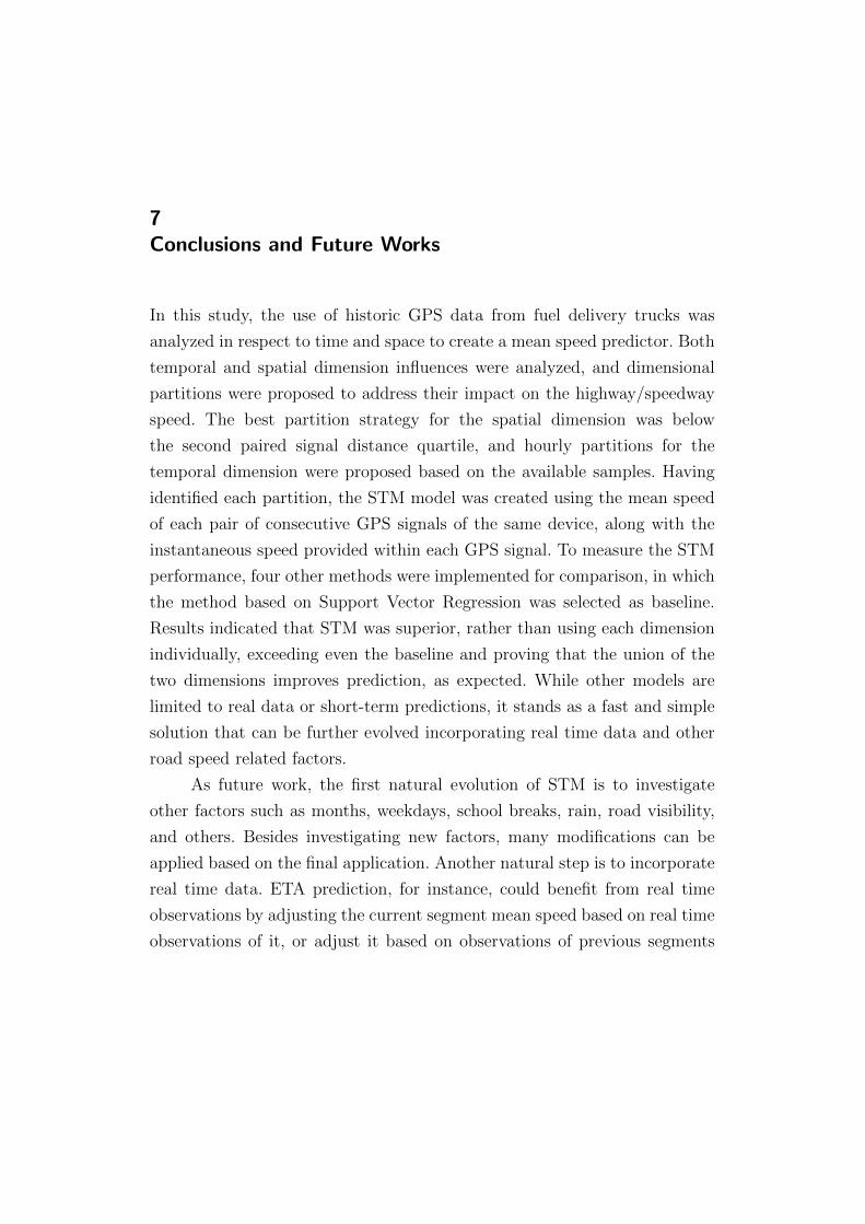
7Conclusions and Future Works
In this study, the use of historic GPS data from fuel delivery trucks was
analyzed in respect to time and space to create a mean speed predictor. Both
temporal and spatial dimension influences were analyzed, and dimensional
partitions were proposed to address their impact on the highway/speedway
speed. The best partition strategy for the spatial dimension was below
the second paired signal distance quartile, and hourly partitions for the
temporal dimension were proposed based on the available samples. Having
identified each partition, the STM model was created using the mean speed
of each pair of consecutive GPS signals of the same device, along with the
instantaneous speed provided within each GPS signal. To measure the STM
performance, four other methods were implemented for comparison, in which
the method based on Support Vector Regression was selected as baseline.
Results indicated that STM was superior, rather than using each dimension
individually, exceeding even the baseline and proving that the union of the
two dimensions improves prediction, as expected. While other models are
limited to real data or short-term predictions, it stands as a fast and simple
solution that can be further evolved incorporating real time data and other
road speed related factors.
As future work, the first natural evolution of STM is to investigate
other factors such as months, weekdays, school breaks, rain, road visibility,
and others. Besides investigating new factors, many modifications can be
applied based on the final application. Another natural step is to incorporate
real time data. ETA prediction, for instance, could benefit from real time
observations by adjusting the current segment mean speed based on real time
observations of it, or adjust it based on observations of previous segments
Chapter 7. Conclusions and Future Works 71
as the travel occurs. Another possible improvement could be to adapt STM
as an analogue model for SVR and ANN. Second-order Route Optimizations
can be another direction of study, using STM to optimize routes based on
predictions, instead of current observed data. Also, an accident detection
framework can be implemented comparing the predicted mean speed to
current mean speeds, if large deviations are identified they may implicate
on a car crash or other random events.
There is a vast range of possible applications and evolutions for STM
since, in general, STM can be used as a base model to be evolved accordingly,
or as a final model to be queried by any highway or speedway traffic related
application. Although room for improvement is always present, STM offers
a satisfactory quality over speed factor.
8Bibliography
AMARAL, B. G. do. A visual analysis of bus GPS data in Rio. Dissertacao
(Mestrado) — PUC-Rio, June 2015.
BAJWA, S.; CHUNG, E.; KUWAHARA, M. An adaptive travel time prediction
model based on pattern matching. In: Proc. of 11th Intelligent Transport
Systems World Congress. [S.l.: s.n.], 2004.
BIN, Y.; ZHONGZHEN, Y.; BAOZHEN, Y. Bus arrival time prediction using
support vector machines. Journal of Intelligent Transportation Systems,
Taylor & Francis, v. 10, n. 4, p. 151–158, 2006.
BRAKATSOULAS, S. et al. On map-matching vehicle tracking data. In: VLDB
ENDOWMENT. Proceedings of the 31st international conference on Very
large data bases. [S.l.], 2005. p. 853–864.
CHAKROBORTY, P.; KIKUCHI, S. Using bus travel time data to estimate
travel times on urban corridors. Transportation Research Record: Journal
of the Transportation Research Board, Transportation Research Board of
the National Academies, n. 1870, p. 18–25, 2004.
CHIEN, S. I.-J.; DING, Y.; WEI, C. Dynamic bus arrival time prediction with
artificial neural networks. Journal of Transportation Engineering, American
Society of Civil Engineers, v. 128, n. 5, p. 429–438, 2002.
CHROBOK, R. et al. Different methods of traffic forecast based on real data.
European Journal of Operational Research, Elsevier, v. 155, n. 3, p.
558–568, 2004.

Chapter 8. Bibliography 73
DEREKENARIS, G. et al. Integrating gis, gps and gsm technologies for the
effective management of ambulances. Computers, Environment and Urban
Systems, Elsevier, v. 25, n. 3, p. 267–278, 2001.
FABRITIIS, C. D.; RAGONA, R.; VALENTI, G. Traffic estimation and prediction
based on real time floating car data. In: IEEE. Intelligent Transportation
Systems, 2008. ITSC 2008. 11th International IEEE Conference on. [S.l.],
2008. p. 197–203.
FAN, R.-E. et al. Liblinear: A library for large linear classification. The Journal
of Machine Learning Research, JMLR. org, v. 9, p. 1871–1874, 2008.
GEORGESCU, L.; ZEITLER, D.; STANDRIDGE, C. R. Intelligent transportation
system real time traffic speed prediction with minimal data. Journal of
Industrial Engineering and Management, v. 5, n. 2, p. 431–441, 2012.
GOPI, G. et al. Bayesian support vector regression for traffic speed prediction
with error bars. In: IEEE. Intelligent Transportation Systems-(ITSC), 2013
16th International IEEE Conference on. [S.l.], 2013. p. 136–141.
HOFMANN-WELLENHOF, B.; LICHTENEGGER, H.; COLLINS, J. Global
positioning system: theory and practice. [S.l.]: Springer Science & Business
Media, 2013.
HOLLANDS, R. G. Will the real smart city please stand up? intelligent,
progressive or entrepreneurial? City, Taylor & Francis, v. 12, n. 3, p. 303–320,
2008.
KAMRAN, S.; HAAS, O. A multilevel traffic incidents detection approach:
Identifying traffic patterns and vehicle behaviours using real-time gps data. In:
IEEE. Intelligent Vehicles Symposium, 2007 IEEE. [S.l.], 2007. p. 912–917.
KIRBY, H. R.; WATSON, S. M.; DOUGHERTY, M. S. Should we use neural
networks or statistical models for short-term motorway traffic forecasting?
International Journal of Forecasting, Elsevier, v. 13, n. 1, p. 43–50, 1997.

Chapter 8. Bibliography 74
KORMAKSSON, M. et al. Bus travel time predictions using additive models.
In: IEEE. Data Mining (ICDM), 2014 IEEE International Conference on.
[S.l.], 2014. p. 875–880.
LEE, W.-H.; TSENG, S.-S.; TSAI, S.-H. A knowledge based real-time travel
time prediction system for urban network. Expert Systems with Applications,
Elsevier, v. 36, n. 3, p. 4239–4247, 2009.
MARK, C. D.; SADEK, A. W.; RIZZO, D. Predicting experienced travel
time with neural networks: a paramics simulation study. In: IEEE. Intelligent
Transportation Systems, 2004. Proceedings. The 7th International IEEE
Conference on. [S.l.], 2004. p. 906–911.
NANTHAWICHIT, C.; NAKATSUJI, T.; SUZUKI, H. Application of
probe-vehicle data for real-time traffic-state estimation and short-term
travel-time prediction on a freeway. Transportation Research Record: Journal
of the Transportation Research Board, Transportation Research Board of the
National Academies, n. 1855, p. 49–59, 2003.
SHALABY, A.; FARHAN, A. Bus travel time prediction model for dynamic
operations control and passenger information systems. Transportation
Research Board, 2003.
STEVEN, I.; CHIEN, J.; KUCHIPUDI, C. M. Dynamic travel time prediction with
real-time and historic data. Journal of transportation engineering, American
Society of Civil Engineers, 2003.
THOMAS, T.; WEIJERMARS, W.; BERKUM, E. V. Predictions of urban
volumes in single time series. Intelligent Transportation Systems, IEEE
Transactions on, IEEE, v. 11, n. 1, p. 71–80, 2010.
TOWNSHEND, A. D.; WORRINGHAM, C. J.; STEWART, I. B. Assessment of
speed and position during human locomotion using nondifferential gps. Medicine
and science in sports and exercise, Citeseer, v. 40, n. 1, p. 124, 2008.
VANAJAKSHI, L.; SUBRAMANIAN, S. C.; SIVANANDAN, R. Travel time
prediction under heterogeneous traffic conditions using global positioning system
Chapter 8. Bibliography 75
data from buses. IET intelligent transport systems, IET, v. 3, n. 1, p. 1–9,
2009.
WU, C.-H.; HO, J.-M.; LEE, D.-T. Travel-time prediction with support vector
regression. Intelligent Transportation Systems, IEEE Transactions on,
IEEE, v. 5, n. 4, p. 276–281, 2004.
YANG, J.-S. Travel time prediction using the gps test vehicle and kalman filtering
techniques. In: IEEE. American Control Conference, 2005. Proceedings of
the 2005. [S.l.], 2005. p. 2128–2133.
YASDI, R. Prediction of road traffic using a neural network approach. Neural
computing & applications, Springer, v. 8, n. 2, p. 135–142, 1999.
YUSUF, A. Advanced machine learning models for online travel-time prediction
on freeways. Georgia Institute of Technology, 2013.
ZHANG, G.; PATUWO, B. E.; HU, M. Y. Forecasting with artificial neural
networks:: The state of the art. International journal of forecasting, Elsevier,
v. 14, n. 1, p. 35–62, 1998.
ZHENG, Y. Trajectory data mining: an overview. ACM Transactions on
Intelligent Systems and Technology (TIST), ACM, v. 6, n. 3, p. 29, 2015.