Embed Size (px)
Citation preview

UNIVERSIDADE DE BRASILIA
FACULDADE DE TECNOLOGIA
DEPARTAMENTO DE ENGENHARIA ELETRICA
SPATIO-TEMPORAL PREDICTION OF ELECTRIC
POWER SYSTEMS INCLUDING EMERGENT
RENEWABLE ENERGY SOURCES
JAYME MILANEZI JUNIOR
ORIENTADOR: JOAO PAULO CARVALHO LUSTOSA DA COSTA
COORIENTADOR: JOSE ANTONIO ALVES GOMES
DISSERTACAO DE MESTRADO EM
ENGENHARIA ELETRICA
PUBLICACAO: 554/2014 DM PPGEE
BRASILIA/DF: MARCO - 2014.


UNIVERSIDADE DE BRASILIA
FACULDADE DE TECNOLOGIA
DEPARTAMENTO DE ENGENHARIA ELETRICA
SPATIO-TEMPORAL PREDICTION OF ELECTRIC
POWER SYSTEMS INCLUDING EMERGENT
RENEWABLE ENERGY SOURCES
JAYME MILANEZI JUNIOR
DISSERTACAO DE MESTRADO SUBMETIDA AO DEPARTAMENTO
DE ENGENHARIA ELETRICA DA FACULDADE DE TECNOLOGIA
DA UNIVERSIDADE DE BRASILIA, COMO PARTE DOS REQUISITOS
NECESSARIOS PARA A OBTENCAO DO GRAU DE MESTRE EM EN-
GENHARIA ELETRICA.
APROVADA POR:
Prof. Joao Paulo C. Lustosa da Costa, Dr.-Ing. (ENE-UnB)
(Orientador)
Prof. Jose Antonio Alves Gomes, Dr. (INPA)
(Coorientador)
Prof. Ricardo Zelenovsky, Dr. (ENE-UnB)
(Examinador Interno)
Fabio Stacke Silva, Dr. (ANEEL)
(Examinador Externo)
BRASILIA-DF, 12 DE MARCO DE 2014.
ii

FICHA CATALOGRAFICA
MILANEZI JR, JAYME
FOLHA CATALOGRAFICA - Spatio-Temporal Prediction of Electric Power
Systems including Emergent Renewable Energy Sources.
[Distrito Federal] 2014.
xxviii, 146p., 297mm (ENE/FT/UnB, Mestre, Engenharia Eletrica, 2014).
Dissertacao de Mestrado - Universidade de Brasılia.
Faculdade de Tecnologia.
Departamento de Engenharia Eletrica.
1. Predicao de Series Temporais 2. Sistemas de Potencia
3. Fontes Alternativas de Energia 4. Processamento de Sinais
I. ENE/FT/UnB II. Publicacao 554/2014 DM PPGEE
REFERENCIA BIBLIOGRAFICA
MILANEZI JR., J. (2014). Spatio-temporal Prediction of Electric Power Systems in-
cluding Emergent Renewable Energy Sources. Dissertacao de Mestrado em Engenharia
Eletrica, Publicacao 554/2014 DM PPGEE, Departamento de Engenharia Eletrica,
Universidade de Brasılia, Brasılia, DF, 146p.
CESSAO DE DIREITOS
NOME DO AUTOR: Jayme Milanezi Junior.
TITULO DA DISSERTACAO DE MESTRADO: Spatio-temporal Prediction of Elec-
tric Power Systems including Emergent Renewable Energy Sources.
GRAU / ANO: Mestre / 2014
O autor permite, desde ja, a reproducao total ou parcial desta dissertacao de mestrado,
desde que seja rigorosamente respeitada a citacao da fonte.
Jayme Milanezi JuniorSQN 409, bloco I,CEP 70857-090 Brasılia - DF - Brasil.
iii

Nao posso imaginar que uma vida sem trabalho seja capaz de trazer qual-
quer especie de conforto. A imaginacao criadora e o trabalho, para mim,
andam de maos dadas; nao retiro prazer de nenhuma outra coisa.
(Sigmund Freud)
iv

DEDICATORIA
A minha esposa, Gal, e aos nossos futuros filhos.
v

AGRADECIMENTOS
A minha esposa, Maria Galberianny, que, com amor, companheirismo e
verdadeira doacao, tolerou meu frequente distanciamento em virtude dos
numerosos trabalhos que empreendi durante este mestrado. A voce, que
sempre confiou na minha capacidade, me apoiando e fortalecendo a minha
moral para este bom combate, agradeco de todo o meu coracao. Amo voce.
Agradeco ao meu orientador e ex-colega de profissao, Prof. Joao Paulo,
com cuja amizade conto desde os tempos em que ombreamos no Instituto
Militar de Engenharia (IME). Enquanto Professor, sempre me dispensou
inestimavel ajuda no ambito do mestrado, tendo me apresentado um insti-
gante e desafiador campo de pesquisa, e dirimindo varias de minhas duvidas
em tempo real. Pelo exemplo e incentivo incansaveis, sou-lhe extremamente
grato.
Aos meus colegas na Agencia Nacional de Energia Eletrica (ANEEL), prin-
cipalmente aos meus companheiros na Superintendencia de Pesquisa e De-
senvolvimento e Eficiencia Energetica (SPE), por terem prestigiado os meus
esforcos ao longo da preparacao desta dissertacao. Ao Superintendente,
Maximo Luiz Pompermayer, agradeco pela confianca em que o meu trabalho
na SPE prosseguiria sem maiores percalcos, mesmo com o desenvolvimento
concomitante das tarefas relacionadas ao mestrado. Igualmente, gostaria
aqui de deixar meus agradecimentos a Aurelio Calheiros Melo Junior, As-
sessor da SPE, por ter sempre demonstrado apoio e incentivo as tarefas
academicas, e aos demais colegas de sala e de toda a ANEEL, que foram
grandes amigos, verdadeiros vetores de renovacao e bom humor ao longo
desta jornada. Um especial agradecimento a Lucas Dantas Xavier Ribeiro,
que veio a se tornar um fundamental colaborador em alguns topicos da pre-
sente dissertacao, auxiliando-me com algumas sintaxes de MATLAB e na
organizacao e processamento de dados em sua distribuicao espacial. Muito
obrigado a todos voces.
Ao meu coorientador, Prof. Jose Antonio Alves Gomes, do Instituto Na-
cional de Pesquisas da Amazonia (INPA), por ter me apoiado com o ar-
cabouco teorico relacionado a um importante vetor energetico que estamos
aqui apresentando como uma possıvel fonte renovavel, as enguias eletricas.
vi

A pesquisadora Renata Schmidt, da Universidade Federal do Amazonas
(UFAM), pela colaboracao dada juntamente com o Prof. Jose Gomes, e ao
Prof. Jose Luiz Cerda-Arias, que nos forneceu os dados de 29 subestacoes
eletricas da cidade de Leipzig - Saxonia, Alemanha, tambem dedico meu
sincero reconhecimento. Deixo aqui tambem um obrigado a Ronaldo Se-
bastiao Ferreira Junior, que me prestou grande auxılio na concepcao de
alguns circuitos para a parte de reciclagem de ondas radio e na propria
parte de reciclagem de luz indoor.
Aos meus colegas em inovacoes tecnologicas e materias de mestrado Marco
Antonio Marques Marinho, Edison Pignaton, Antonio Rubio Serrano, Danilo
Fernandes, Bruno Pilon, Ricardo Kehrle e Stephanie Alvarez, agradeco pela
parceria, seja nos estudos em conjunto, seja naqueles debates teoricos sobre
os modelos estudados, cujas discussoes sempre foram da maior relevancia,
sempre por demais construtivas. Ao Prof. Ricardo Zelenovsky e a Fabio
Stacke Silva, integrantes da banca avaliadora, sou grato pelas valorosas re-
visoes do texto final desta dissertacao, as quais tornaram o texto de leitura
sem duvida mais aprazıvel.
Aos meus pais, Jayme e Lucia, que, com amor e paciencia, me deram desde
cedo o ensinamento de que o estudo, a honestidade e a superacao pessoal
moldam os unicos caminhos que edificam e valorizam permanentemente
nossas vidas. Aos meus irmaos Pollyanna, Marcos e Thiago, pelo suporte
emocional e conversas revigorantes. Voces sao um grande esteio de carinho
e amparo na minha vida.
Agradeco, por fim...
... a Deus, se ele existir.
vii

RESUMO
PREDICAO ESPACIAL TEMPORAL DE SISTEMAS ELETRICOS DE
POTENCIA INCLUINDO FONTES RENOVAVEIS EMERGENTES
Autor: Jayme Milanezi Junior
Orientador: Joao Paulo Carvalho Lustosa da Costa
Coorientador: Jose Antonio Alves Gomes
Programa de Pos-graduacao em Engenharia Eletrica
Brasılia, marco de 2014
A atividade de planejamento de sistemas de potencia inclui, como um de seus maiores
desafios, a predicao do comportamento da carga. Com a finalidade de otimizar o
investimento ante os dados de consumo, as empresas do setor eletrico lancam mao de
varias tecnicas de previsao da evolucao da demanda que devem atender. No presente
trabalho, o tema da predicao espacial e temporal da carga e enfrentado, estudando e
incorporando, simultaneamente, a tendencia hoje ja observada de inclusao de fontes
em microgeracao distribuıda. Tres fontes renovaveis e emergentes de geracao foram
consideradas como geradoras de energia pelos consumidores: enguias eletricas, paineis
fotovoltaicos para aproveitamento da luz solar e de interiores, e antenas para reciclagem
da energia existente nas ondas eletromagneticas de radiodifusao. Quatro metodos
preditivos foram empregados para prever o comportamento da carga: modelo Auto-
Regressivo (AR), Auto-Regressivo com Variavel eXogena (ARX), Auto-Regressivo de
Media Movel com Variavel eXogena (ARMAX) e Redes Neurais Artificiais (ANN). Os
dados de consumo foram as maximas demandas semanais registradas em 8 Subestacoes
da cidade de Leipzig (Saxonia, Alemanha), durante os anos de 2001, 2002, 2003 e 2004.
O dado exogeno considerado foi a temperatura, em valores diretos e logarıtmicos. Das
209 semanas existentes entre 2001 e 2004, as 200 primeiras destinaram-se ao ajuste dos
coeficientes nos modelos AR e ao treinamento da rede neural; as 9 semanas restantes
foram destinadas a comparacao de resultados. A aplicacao das tecnicas deu-se, assim,
em dois estagios: no primeiro, os dados reais da rede de Leipzig foram considerados, e
no segundo estagio trabalhou-se com novos valores de demandas maximas, originadas
pela insercao de valores hipoteticos de energia recebida das tres fontes citadas. Em
ambos os estagios, o modelo ARMAX foi o de melhor precisao na previsao de dados.
O sistema de redes neurais demonstrou ser um sistema sub-otimo de previsao.
Palavras Chave: Predicao de Series Temporais, ARMAX, Redes Neurais, Geracao por
Enguias Eletricas, Reciclagem de Energia.
viii

ABSTRACT
SPATIO-TEMPORAL PREDICTION OF ELECTRIC POWER SYSTEMS
INCLUDING EMERGENT RENEWABLE ENERGY SOURCES
Author: Jayme Milanezi Junior
Supervisor: Joao Paulo Carvalho Lustosa da Costa
Co-supervisor: Jose Antonio Alves Gomes
Programa de Pos-graduacao em Engenharia Eletrica
Brasılia, March of 2014
Power systems planning activities include load behavior prediction as one of its most
challenging tasks. In order to optmize investments related to consumption data, util-
ities from the Electrical Sector resort to several forecasting techniques so that they
can predict the power demand which these utilities must support. Along the present
work, issues related to the spatial and temporal predictions are faced, considering,
simultaneously, the observed trend of microgeneration spread. Three emergent renew-
able sources were proposed to be taken on by consumers: electric eels, photovoltaic
solar panels for outdoor generation and indoor light energy harvesting, and antennas
for radio frequency energy recycling. Four predictive methods were employed in order
to forecast load evolution: Auto-Regressive (AR), Auto-Regressive with eXogeneous
inputs (ARX), Auto-Regressive Moving Average with eXogeneous inputs (ARMAX)
models and Artificial Neural Networks (ANN). Consumption data were the maximum
weekly power demands registered over 8 Power Substations from the city of Leipzig
(Saxony, Germany), during the years 2001, 2002, 2003 and 2004. The exogeneous
variable adopted was temperature, in realistic and in logarithmic values. During the
209 weeks which are comprised between 2001 and 2004, the first 200 weeks served to
coefficients adjustments, with regards to AR models, and the trainning of the neural
network, in the case of ANN. The last 9 weeks were destinated for results compari-
son. Techniques were undertaken in two stages: firstly, only realistic data from Leipzig
Substations were considered, and in the second stage, new values for maximum power
demands were obtained by means of simulations upon the three emergent sources. In
both stages, ARMAX model returned the fittest results, whereas ANN characterized
itself as a sub-optimal prediction system.
Keywords: Time Series Prediction, ARMAX, Artificial Neural Networks, Electric Eels
Generation, Energy Recycling.
ix

x

Contents
1 INTRODUCAO 1
1.1 Motivacao . . . . . . . . . . . . . . . . . . . . . . . . . . . . . . . . . . 1
1.2 Premissas e Objetivos . . . . . . . . . . . . . . . . . . . . . . . . . . . 3
1.3 Como esta Dissertacao esta Organizada . . . . . . . . . . . . . . . . . . 8
2 INTRODUCTION 1
2.1 Motivation . . . . . . . . . . . . . . . . . . . . . . . . . . . . . . . . . . 1
2.2 Premises and Objectives . . . . . . . . . . . . . . . . . . . . . . . . . . 3
2.3 How this Dissertation is Organized . . . . . . . . . . . . . . . . . . . . 7
3 EMERGENT RENEWABLE SOURCES 10
3.1 RF Energy Harvesting . . . . . . . . . . . . . . . . . . . . . . . . . . . 10
3.1.1 Theory and State of the Art . . . . . . . . . . . . . . . . . . . . 10
3.1.2 Measurements . . . . . . . . . . . . . . . . . . . . . . . . . . . . 15
3.1.3 Expected results given the measurements . . . . . . . . . . . . . 18
3.2 Indoor Light Energy Recycling . . . . . . . . . . . . . . . . . . . . . . . 19
3.2.1 Theory and State of the Art . . . . . . . . . . . . . . . . . . . . 19
3.2.2 Open Circuit and Short Circuit Measurements in Indoor Envi-
ronments for the a-Si Panel . . . . . . . . . . . . . . . . . . . . 20
3.2.3 Charge Profile of a Cell Phone Battery . . . . . . . . . . . . . . 23
3.2.4 Indoor Experiment Using Artificial Light and Results . . . . . . 26
3.2.5 Expected results for outdoor environments . . . . . . . . . . . . 30
3.3 Electric Eel . . . . . . . . . . . . . . . . . . . . . . . . . . . . . . . . . 31
3.3.1 Theory . . . . . . . . . . . . . . . . . . . . . . . . . . . . . . . . 31
3.3.2 State of the Art . . . . . . . . . . . . . . . . . . . . . . . . . . . 32
3.3.3 Measurements . . . . . . . . . . . . . . . . . . . . . . . . . . . . 35
3.4 Summary of the three energetic sources . . . . . . . . . . . . . . . . . . 43
4 ENERGY DEMAND PREDICTION IN A STANDARD ELECTRIC
POWER GRID 44
4.1 Overview . . . . . . . . . . . . . . . . . . . . . . . . . . . . . . . . . . . 44
xi
4.1.1 AR, ARX and ARMAX Models . . . . . . . . . . . . . . . . . . 48
4.1.2 Artificial Neural Networks . . . . . . . . . . . . . . . . . . . . . 50
4.1.3 Comparison Between AR, ARX, ARMAX and ANN Results . . 51
4.2 Leipzig Map for the Power Substations . . . . . . . . . . . . . . . . . . 57
5 ENERGY DEMAND PREDICTION INCLUDING RENEWABLE
ENERGY GENERATION 60
5.1 Parameters of Temporal Evolution for Renewable Sources . . . . . . . . 61
5.1.1 Panels and antennas growing rates . . . . . . . . . . . . . . . . 62
5.1.2 Electric Eels Aquariums in the River . . . . . . . . . . . . . . . 66
5.1.3 Unilateral white noise upon constant values: the k factor . . . . 66
5.1.4 Results for PV panels and antennas . . . . . . . . . . . . . . . . 68
5.2 Forecasting overall results considering power micro-generation values . 69
5.2.1 Solar PV Panels Generating Outdoor and Indoor . . . . . . . . 69
5.2.2 Solar PV Panels Generating Only Indoor . . . . . . . . . . . . . 76
5.2.3 Generating Only with Eels and Antennas . . . . . . . . . . . . . 78
5.3 Spatial Forecast . . . . . . . . . . . . . . . . . . . . . . . . . . . . . . . 80
6 CONCLUSIONS 86
APPENDICES 97
A Stationary Processes 98
A.1 Discrete-Time Stochastic Processes . . . . . . . . . . . . . . . . . . . . 98
A.1.1 Statistical Functions with Respect to Only One Random Variable 100
A.1.2 Statistical Functions with Respect to More than One Random
Variable . . . . . . . . . . . . . . . . . . . . . . . . . . . . . . . 105
A.2 Stationarity - Examples . . . . . . . . . . . . . . . . . . . . . . . . . . 111
A.2.1 Non-Stationary Processes - the Neighbours Musicians . . . . . . 111
A.2.2 Example of a Stationary Series . . . . . . . . . . . . . . . . . . 114
A.2.3 Ergodicity . . . . . . . . . . . . . . . . . . . . . . . . . . . . . . 116
B Z-Transform Models 118
B.1 Background: Z-transform . . . . . . . . . . . . . . . . . . . . . . . . . 119
B.1.1 Definition . . . . . . . . . . . . . . . . . . . . . . . . . . . . . . 119
B.1.2 Region of Convergence (ROC) . . . . . . . . . . . . . . . . . . . 120
B.1.3 Behavior of z . . . . . . . . . . . . . . . . . . . . . . . . . . . . 121
B.1.4 Time-delayed data . . . . . . . . . . . . . . . . . . . . . . . . . 122
B.1.5 Z-Transform Properties . . . . . . . . . . . . . . . . . . . . . . 123
xii

B.2 Z-Filters . . . . . . . . . . . . . . . . . . . . . . . . . . . . . . . . . . . 125
B.2.1 Infinite Impulse Response (IIR) and Finite Impulse Response (FIR)128
B.2.2 Forecasted Error Model (FEM) . . . . . . . . . . . . . . . . . . 130
B.2.3 AR(X) and MA Models . . . . . . . . . . . . . . . . . . . . . . 132
C Examples of Peak Load Reductions over the Substations in Leipzig
Map 135
xiii

List of Tables
1.1 Oferta Interna de Energia (OIE), Produto Interno Bruto (PIB) e Pop-
ulacao, de 2003 a 2012, no Brasil [4] . . . . . . . . . . . . . . . . . . . . 2
2.1 Domestric Energy Supply (DES), Gross Domestic Product (GDP) and
Population from 2003 to 2012 in Brazil [4] . . . . . . . . . . . . . . . . 2
3.1 Frequency bands of energy harvesting and respective maximum dBm
power . . . . . . . . . . . . . . . . . . . . . . . . . . . . . . . . . . . . 13
3.2 Incident power as a function of dBm values - examples . . . . . . . . . 19
3.3 Maximal Efficiency Values for Crystalline Silicon, Amorphous Silicon,
and Organic BHJ Solar Cells under different spectral illumination [24]. 20
3.4 Annual Average of Daily Irradiance [Wh/m2] by Brazilian Region [40]. 31
3.5 Summary about three energetic sources: RF harvesters, indoor light
recycling, electric eels. . . . . . . . . . . . . . . . . . . . . . . . . . . . 43
4.1 AR and ARX models performances in terms of prediction focus and
FPE, considering temperature and log temperature as eXogeneous vari-
ables in ARX cases. . . . . . . . . . . . . . . . . . . . . . . . . . . . . . 50
4.2 Mean Square Errors (MSE) and Number of Positive Deviations (NPD)
for AR, ARX, ARX log[T] and ARMAX log[T], na = 10, nb = 10 and
nk = 1 . . . . . . . . . . . . . . . . . . . . . . . . . . . . . . . . . . . . 52
5.1 MSE for AR, ARX, ARX log[T], ARMAX and ANN, and the best num-
ber of hidden layers for ANN system in function of each combination of
w, a and k, for periods of 35 and 50 weeks. . . . . . . . . . . . . . . . . 71
5.2 MSE for AR, ARX, ARX log[T], ARMAX and ANN, and the best num-
ber of hidden layers for ANN system in function of each combination of
w, a and k, for periods of 65 and 80 weeks. . . . . . . . . . . . . . . . . 72
5.3 MSE for AR, ARX, ARX log[T], ARMAX and ANN, and the best num-
ber of hidden layers for ANN system in function of each combination of
w, a and k, for periods of 105 and 120 weeks. . . . . . . . . . . . . . . 74
xiv

5.4 MSE for AR, ARX, ARX log[T], ARMAX and ANN, and the best num-
ber of hidden layers for ANN system in function of each combination of
w, a and k, for periods of 135 and 150 weeks. . . . . . . . . . . . . . . 75
5.5 Number of cases in which a model achieves the best approximation,
taking into account all cases that obbey to the criterion on the left
column. . . . . . . . . . . . . . . . . . . . . . . . . . . . . . . . . . . . 76
xv
List of Figures
1.1 Esquema reduzido do sistema eletrico, compreendendo geradores hidreletricos
distantes, longas linhas de transmissao, distribuicao e consumo . . . . . 4
1.2 Esquema da Fig. 1.1, agora incluindo enguias eletricas nadando em um
rio e recicladores RF sobre as casas, ambos fornecendo energia para o
sistema eletrico interligado, enquanto um analisador de dados reune os
dados de consumo das Subestacoes envolvidas . . . . . . . . . . . . . . 5
1.3 Comparacao entre as redes com e sem microgeradores distribuıdos: a
pessoa representa os geradores, a corda e comparada com as linhas de
transmissao, um bloco pesado representa a carga, e o contrapeso auxiliar
representa a microgeracao: (a) a pessoa efetua o esforco sozinha, e (b)
o esforco de sustentar a carga e parcialmente dividido entre ela e o
contrapeso auxiliar. . . . . . . . . . . . . . . . . . . . . . . . . . . . . . 5
2.1 Reduced scheme of the electric system, comprehending far away hydro-
generators, long transmission lines, distribution and consumption. . . . 4
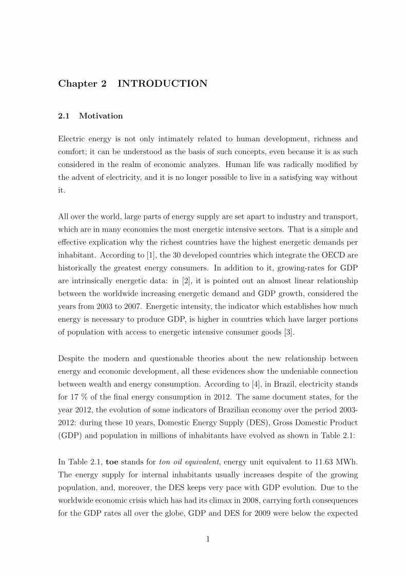
2.2 Scheme of Fig. 1.1, now including eels into the river and an RF recycler
on top of houses, both delivering generating power for the interconnected
power system, while a data analyzer gathers up the consumption data
from the Power Substations. . . . . . . . . . . . . . . . . . . . . . . . . 5
2.3 Comparison of the grid with micro-generators: the man represents gen-
erators, the rope is compared to transmission lines, a heavy block repre-
sents the load, and the auxiliary counterweight stands for the renewable
sources: (a) the man pulls it alone, and (b) the burden of load is partially
shared between him and the auxiliary weight. . . . . . . . . . . . . . . 5
3.1 Components of a RF energy harvesting system: the rectenna is an an-
tenna with a RF-DC interface [5]. Therefore, the receiver must be inte-
grated to a matching circuit, a voltage booster and the rectifier, whose
output is often connected to a battery. . . . . . . . . . . . . . . . . . . 11
3.2 Resulting Vout according to input dBm [6]. . . . . . . . . . . . . . . . . 14
3.3 End-to-end efficiencies for ambient RF energy harvesting [7]. . . . . . . 15
xvi
3.4 Map of Brasilia-DF (Brazil) with the indicated 4 places on which RF
spectrum intensities were measured. . . . . . . . . . . . . . . . . . . . . 16
3.5 Measurements of incident dBm power according to frequency. Each
place encloses morning, afternoon and evening data, which are mixed in
each graph. . . . . . . . . . . . . . . . . . . . . . . . . . . . . . . . . . 17
3.6 Results which overcome -15 dBm, here called “best results”, with values
properly signalized in order to show participation of each place in this
group. . . . . . . . . . . . . . . . . . . . . . . . . . . . . . . . . . . . . 18
3.7 Typical solar light AM 1.5 and cold-cathode fluorescent light spectra. . 21
3.8 Absorbed Light Intensity Lx [lux] versus Open Circuit Voltage Voc [V]
of the solar panel 95 mm x 110 mm for a LED 8 W lamp. . . . . . . . . 22
3.9 Absorbed Light Intensity Lx [lux] versus Short Circuit Current Isc [mA]
of a solar panel 95 mm x 110 mm for a LED 8 W lamp. . . . . . . . . . 22
3.10 Current and voltage versus time of a cell phone charging at 220 V, 60 Hz. 23
3.11 Apparent Impedance (Ω) of cell phone seen by the source. . . . . . . . 25
3.12 Instantaneous transferred power to the cell phone as seen by the source. 25
3.13 Overall deployment of cell phone, amperimeter (in series) and solar panel
under a light-support in an office for electrical current measurement. . . 26
3.14 Designed boost converter producing 5 V in steady state . . . . . . . . . 27
3.15 Effective voltage and current in steady state over a load of resistive load
R of 50 Ω. . . . . . . . . . . . . . . . . . . . . . . . . . . . . . . . . . . 29
3.16 Bars indicating equal periods of time A and B as demonstration that
transferred power is influenced by resistance (PB>PA). . . . . . . . . . 29
3.17 Electrocytes behavior which yields an external electric voltage: (a) cell
membrane is permeable only to K+ ions; (b) Acetylcholine activates the
electrocyte cell, making Na+ ions to come inside it [43]. In the case
of Electrophorus electricus, there exists only the posterior membrane,
which is excitable. . . . . . . . . . . . . . . . . . . . . . . . . . . . . . . 33
3.18 Lines of electric field generated along the eel’s body. The head is the
positive pole, and the tail bears the negative pole, from where electric
current goes off through water until the head [44]. . . . . . . . . . . . . 34
3.19 Equivalent circuit of the electric eel [45]. . . . . . . . . . . . . . . . . . 34
3.20 Real experiment carried out in LFCE-INPA, wherein the electrodes are
metal plaques with a resistance of 4 Ω each. This photo was made while
the electric eel swam in order to look for the prey, which is the little fish
in the above part of the aquarium, near to the surface. . . . . . . . . . 35
xvii

3.21 Picture which outlines the overall deployment of the experiment: two
metal plaques actuating as electrodes were placed on each side of the
largest width, which is 120 cm. Two resistances were then purposefully
inserted in the part of circuit the voltimeter was connected. . . . . . . . 36
3.22 Equivalent circuit of Fig. 3.21, illustrating the eel as the voltage source.
Ra is the varying water resistance, and 8 Ω corresponds to the total
electrodes resistances in series. The resistances of 3 Ω were inserted to
protect the voltimeter and to improve measuring accuracy. . . . . . . . 36
3.23 Voltage values with the eel swimming freely into the aquarium. . . . . . 37
3.24 Voltage values with (a) the eel being stressed, and (b) eel trying to kill
a little prey that is placed in the aquarium. . . . . . . . . . . . . . . . . 39
3.25 Perspective view of the basket, or aquarium-corral. The brown lines
represent conductors, either nude cable or bars, each one being connected
to a different polarity of the external circuit of power management. . . 40
3.26 Upper views of the basket: (a) view of the basket without eels inside;
(b) view of the basket with one eel swimming inside the corral. At any
moment of the displacement of the eel, both head and tail are likely to
be near to the collecting current points, which are the conductive cables. 41
3.27 Proposed scheme for energy harvesting from eels in a river, which com-
prises eels inside the baskets. All the output cables are connected to a
power manager circuit, which carries out this power to be conditioned. 42
4.1 Visual representation of the set of values which influences the next fore-
casted output y(t) at each moment: underlining (a) values which in-
fluence output y(k + 5) and, and in the next instant, (b) values which
influence y(k + 6). . . . . . . . . . . . . . . . . . . . . . . . . . . . . . 45
4.2 Maximum electric power demands over the 209 weeks: letters on the top
indicate the PS. Yellow bar on H substation graph shows the forecasted
period for every PS. . . . . . . . . . . . . . . . . . . . . . . . . . . . . . 47
4.3 Models which have provided the minor deviation absolute values, for
each week and PS. . . . . . . . . . . . . . . . . . . . . . . . . . . . . . 52
4.4 Absolute deviation values from Fig. 4.2 divided by the respective mea-
sured values, in percentages . . . . . . . . . . . . . . . . . . . . . . . . 53
4.5 Score of minor deviation absolute values, matching ARX log[T] versus
ANN, for each week and PS . . . . . . . . . . . . . . . . . . . . . . . . 54
4.6 Score of minor deviation absolute values, from the match ARMAX log[T]
versus ARX log[T], for each week and PS . . . . . . . . . . . . . . . . . 54
xviii
4.7 Measured data and forecast data for Power Substation D (3092), during
the 9 last weeks of 2004. . . . . . . . . . . . . . . . . . . . . . . . . . . 55
4.8 Measured data and forecast data for Power Substations A, B, C, E, F,
G and H during the 9 last weeks of 2004. . . . . . . . . . . . . . . . . . 56
4.9 ARMAX forecasted maximum electric power demands for 2005 and
2006, for every PS: the blue line relates to measured data, whereas red
lines describe ARMAX prediction data. . . . . . . . . . . . . . . . . . . 58
4.10 Leipzig Map with the 8 Power Stations located [52]. . . . . . . . . . . . 59
5.1 Example of electric demand series: d1 is the overall demand from con-
sumers, d2 is the energy the PS furnishes, and Pµg is the power micro-
generation, so that Pµg = d1 − d2. . . . . . . . . . . . . . . . . . . . . . 61
5.2 (a) Increasing annual data for cell phones in Brazil since 1990; (b) In-
creasing annual data for cable TV in Brazil since 1993 (Anatel). . . . . 62
5.3 Two curves expressing temporal evolution parameters for different sources. 63
5.4 Evolution of grid-connected and off-grid PV panels, in MW (IEA PVPS),
in Japan. . . . . . . . . . . . . . . . . . . . . . . . . . . . . . . . . . . . 64
5.5 Diagram for the routine by which unilateral white noise k is inserted
into original exponential series. . . . . . . . . . . . . . . . . . . . . . . 67
5.6 Global rate over two years, firstly considering pure exponential e0.025t
evolution (a), and then handling values with oscillation upon e0.025t (b).
These last values are believed to be more probable into the market en-
vironment. . . . . . . . . . . . . . . . . . . . . . . . . . . . . . . . . . . 67
5.7 Weekly actual values of square meter PV panels and RF antennas for
the initial value of 50 m2 in the considered PS. . . . . . . . . . . . . . . 68
5.8 New version for Fig. 4.6, now adopting w = 104, a = 2.0, k = 2.5 and
c = 50. Realistic Data corresponds to Measured Data from Fig. 4.6. . . 77
5.9 New version for Fig. 4.6, now adopting w = 104, a = 2.0, k = 2.5 and
c = 50. Realistic data corresponds to measured data from Fig. 4.7. . . 78
5.10 Curves of demand with no sources generating, with the three sources
and with only eels and RF antennas. . . . . . . . . . . . . . . . . . . . 78
5.11 Antennas generating from January 2002, initial quantity of 300 anten-
nas, increasing rate 172% for year, providing the tiny gap which is ob-
served only in 2006 months. . . . . . . . . . . . . . . . . . . . . . . . . 79
5.12 Eels generating from January 2002, initial quantity of 50 and 100 eels,
increasing rate 123% for year, providing the tiny gap which is observed
in the end of 2006. . . . . . . . . . . . . . . . . . . . . . . . . . . . . . 80
5.13 Color codes for the weekly peak load relief percentages. . . . . . . . . . 81
xix

5.14 Simulation with ca = 50, aa = 0.3; ci = 20, ai = 0.1; co = 10, ao = 0.1;
and ce = 100, ae = 0.2, for the last week of 2005. . . . . . . . . . . . . . 82
5.15 New simulation for scenario of Fig. 5.3, now setting all a = 0.2. . . . . . 82
5.16 Scenario of Fig. 5.3, this time for the last week of 2006. . . . . . . . . . 83
5.17 Peak load reductions for all Substations for the last week of 2006 and
all a = 0.3. . . . . . . . . . . . . . . . . . . . . . . . . . . . . . . . . . . 84
5.18 Scenario of Fig. 5.17, now considering the initial amount of outdoor
panels being co = 20. . . . . . . . . . . . . . . . . . . . . . . . . . . . . 84
A.1 Three graphics with comparison of Convolution (a) with Cross-Correlation
(b) and Auto-Correlation (c) [57]. . . . . . . . . . . . . . . . . . . . . . 111
A.2 Neighbours musicians, playing according to their own studying routines. 113
A.3 PMF of the first 20000 decimal numerals of π. . . . . . . . . . . . . . . 114
A.4 PMF of the sum of each two numerals side by side, among the first 20000
decimal numerals of π. . . . . . . . . . . . . . . . . . . . . . . . . . . . 115
A.5 PMFs of the sum of each three numerals (a) and four numerals (b) side
by side, among the first 20000 decimal numerals of π. . . . . . . . . . . 116
B.1 Relationship among z-plane and s-plane points. . . . . . . . . . . . . . 121
B.2 Behavior of z, depending on |z| and d: (a) |z| < 1, positive exponent
(clockwise); (b) |z| > 1, positive exponent; (c) |z| > 1, negative exponent
(anti-clockwise). . . . . . . . . . . . . . . . . . . . . . . . . . . . . . . . 122
B.3 Linear Filter of ψi weights. . . . . . . . . . . . . . . . . . . . . . . . . . 125
B.4 General System for Stochastic and Deterministic Inputs [65]. . . . . . . 127
B.5 Infinite Impulse Response (IIR) Digital Filter [63]. . . . . . . . . . . . . 128
C.1 Peak load reduction by district for the last week of 2006, c = 500 and a
= 0.6, antennas only. . . . . . . . . . . . . . . . . . . . . . . . . . . . . 135
C.2 Peak load reduction by district for the last week of 2006, c = 1500 and
a = 1.0, antennas only. . . . . . . . . . . . . . . . . . . . . . . . . . . . 136
C.3 Peak load reduction by district for the last week of 2006, c = 1500 and
a = 1.0 for antennas, c = 200 and a = 1.0 for eels. . . . . . . . . . . . . 136
C.4 Peak load reduction by district for the last week of 2006, c = 300 and a
= 1.0, eels only. . . . . . . . . . . . . . . . . . . . . . . . . . . . . . . . 137
C.5 Peak load reduction by district for the last week of 2006, c = 300 and a
= 1.1, eels only. . . . . . . . . . . . . . . . . . . . . . . . . . . . . . . . 137
C.6 Peak load reduction by district for the last week of 2006, c = 300 and a
= 1.2, eels only. . . . . . . . . . . . . . . . . . . . . . . . . . . . . . . . 138
xx

C.7 Peak load reduction by district for the last week of 2006, c = 50 and a
= 0.6, indoor panels only. . . . . . . . . . . . . . . . . . . . . . . . . . 138
C.8 Peak load reduction by district for the last week of 2006, c = 50 and a
= 0.7, indoor panels only. . . . . . . . . . . . . . . . . . . . . . . . . . 139
C.9 Peak load reduction by district for the last week of 2006, c = 50 and a
= 0.8, indoor panels only. . . . . . . . . . . . . . . . . . . . . . . . . . 139
C.10 Peak load reduction by district for the last week of 2006, c = 50 and a
= 0.9, indoor panels only. . . . . . . . . . . . . . . . . . . . . . . . . . 140
C.11 Peak load reduction by district for the last week of 2006, c = 50 and a
= 1.0, indoor panels only. . . . . . . . . . . . . . . . . . . . . . . . . . 140
C.12 Peak load reduction by district for the last week of 2006, c = 50 and a
= 1.2, indoor panels only. . . . . . . . . . . . . . . . . . . . . . . . . . 141
C.13 Peak load reduction by district for the last week of 2005, c = 50 and a
= 1.2, indoor panels only. . . . . . . . . . . . . . . . . . . . . . . . . . 141
C.14 Peak load reduction by district for the last week of 2005, c = 50 and a
= 1.0, indoor panels only. . . . . . . . . . . . . . . . . . . . . . . . . . 142
C.15 Peak load reduction by district for the last week of 2006, c = 5 and a =
0.2, outoor panels only. . . . . . . . . . . . . . . . . . . . . . . . . . . . 142
C.16 Peak load reduction by district for the last week of 2006, c = 5 and a =
0.3, outoor panels only. . . . . . . . . . . . . . . . . . . . . . . . . . . . 143
C.17 Peak load reduction by district for the last week of 2006, c = 5 and a =
0.4, outoor panels only. . . . . . . . . . . . . . . . . . . . . . . . . . . . 143
C.18 Peak load reduction by district for the last week of 2006, c = 10 and a
= 0.4, outoor panels only. . . . . . . . . . . . . . . . . . . . . . . . . . 144
C.19 Peak load reduction by district for the last week of 2006, c = 15 and a
= 0.4, outoor panels only. . . . . . . . . . . . . . . . . . . . . . . . . . 144
C.20 Peak load reduction by district for the last week of 2006, c = 20 and a
= 0.4, outoor panels only. . . . . . . . . . . . . . . . . . . . . . . . . . 145
C.21 Peak load reduction by district for the last week of 2006, c = 20 and a
= 0.3, outoor panels only. . . . . . . . . . . . . . . . . . . . . . . . . . 145
C.22 Peak load reduction by district for the last week of 2005, c = 20 and a
= 0.3, outoor panels only. . . . . . . . . . . . . . . . . . . . . . . . . . 146
C.23 Peak load reduction by district for the last week of 2005, c = 15 and a
= 0.3, outoor panels only. . . . . . . . . . . . . . . . . . . . . . . . . . 146
xxi

List of Symbols, Nomenclatures and Abbreviations
a, an: Logarithmic value of annual increasing rate
Aem: Maximum effective irradiation area
AM: Air Mass
ANATEL: Agencia Nacional de Telecomunicacoes
ANEEL: Agencia Nacional de Energia Eletrica
ANN: Artificial Neural Networks
AR: Auto-Regressive Model
ARMAX: Auto-Regressive Moving Average with eXogeneous Elements
ARMAX-AIC: ARMAX Akaikepsilas Information Criterion
ARMAX-FPE: ARMAX Akaikepsilas Final Prediction Error
ARMAX-NSSE: ARMAX Normalized Sum of Squared Error
ARX: Auto-Regressive with eXogeneous Elements Model
ARX log[T]: Auto-Regressive with eXogeneous Elements Model; the exogeneous ele-
ment, or input, is logarithmic values of minimum weekly temperatures.
a-Si: Amorphous Silicon
A(z): z-polinomyal transfer function related to the AR part, whose input is past values
of Y (z)
BHJ: Bulk Heterojunctions
B(z): z-polinomyal concerning to the eXogeneous part
C1, C2: Capacitors for the boost converter circuit
CCFL: Cold-Cathode Fluorescent Lamp
CFL: Compact Fluorescent Lamp
ci,k, cos(θi,k), ρXiXk: Sample correlation coefficient, or correlation coefficient
xxii

cn, c: Initial amount of the unit generation: antenna, eel or square meter of PV panel
Cov X, Y , σXY : Covariance of X and Y
c-Si: Crystalline Silicon
cx,y, cos(θx,y), ρxy: Correlation coefficient of X and Y
C(z): z-polinomyal concerning to the MA part
D0: Maximum directivity considering the irradiation pattern of the antenna
D1, D2, D3: Diodes for the boost converter circuit
d1: Realistic power demand void of generating sources (example)
d2: Realistic power demand with generating sources (example)
DC: Direct Current
di, dj: Deviation matrix or deviation vector
DTV: Digital Television
e: natural logarithmic basis: e = 2.71828182846...
eα: absolute value of z
ecd: Iradiation efficiency of the antenna
e(t), e(n): noise signal values
Eu[n], µn, µ(n), u[n]: Mean or Expected Value of n
FEM: Forecasted Error Method
f ? f : Autocorrelation function of the PMF f
f ? g: Cross-correlation function of the PMFs f and g
f ∗ g: Convolution function of the PMFs f and g
FIR: Finite Impulse Response filter
Fs: Switching frequency of the converter
xxiii

F (z): z-transform of the function f(x)
g, gt: Power microgeneration actuating on the t-th week
Gr: Gain of the receiver antenna
GSM: Global System for Mobile communications
Gt: Gain of the transmitter antenna
G(z): transfer function related to the eXogeneous part, whose input is U(z)
H(z): transfer function related to the MA part, whose input is W (z)
IEEE: Institute of Electrical and Electronics Engineers
IIR: Infinite Impulse Response filter
Imax: Maximum current
Iout: Current flowing over the output terminals of the circuit
Isc: Short Circuit Current
k: noise summed to an originally pure ascendant exponential, conferring a step-shape
for it
Kind: Estimated coeffcient for the inductor ripple current relative to the maximum
output current
L: Boost converter inductance
LED: Light Emitter Diode
LFCE-INPA: Laboratorio de Fisiologia Comportamental e Evolucao do Instituto Na-
cional de Pesquisas da Amazonia
log[T ]: Logarithmic value of the minimum registered temperature for a week
Lx: Light intensity, in Lux
MDL: Minimum Description Length
MPP: Maximum Power Point
xxiv

Mpv: Number of square meter of PV panels generating power
Mnpv: Number of square meter of PV panels generating power in the n− th week
MSE: Minimum Square Error
na: Number of past output values which are input of the AR filter
nb: Number of past eXogeneous values which are input of the X filter
nc: Number of past noise values which are input of the MA filter
ne: Number of eels
nk: Number of delay instants betwen the forecasted moment and the first exogeneous
value in the future
NPD: Number of Positive Deviations
OECD: Organization for Economic Cooperation and Development
OPV: Organic Photovoltaic Cell
P3HT: Poly-3-hexyl Thiophene
PCBM: Phenyl-C61-Butyric Acid Methyl Ester
PDF: Probability Density Function
Pe: Amount of power produced by the eels
Pe−peak: Power delivered by the batteries only during the peak
PMF: Probability Mass Function
Pµg: Power microgeneration, corresponding to the difference between d1 and d2
Pr: Effective power in the receiver antenna
PS: Power Substation
PSs: Power Substations
Pt: Power transmitted by the transmitter antenna
xxv

Ptm: Maximum power available from a transmitter antenna
PV: Photovoltaic
q−1: delay-shift operator, such that y(t).q−1 = y(t− 1)
R2: Determination Coefficient
Ra: Water resistance
RF: Radio Frequency
ROC: Region of Convergence
RXX : Correlation between dimensions of vector X
rX,Y (t, t+ τ), σXY (τ): Cross-covariance function between X(t) and Y (t), lag of τ
STC: Standard Test Conditions
T : Temperature, or the minimum registered temperature for a week
t: Time, in weeks, from the moment in which the first source unit started to generate
UMTS: Universal Mobile Telecommunications System
u(n), u(t), u: deterministic signal values
U(z): deterministic input data
Var X, σ2X : Variance of X
Vi, Vin: Voltage along the input terminals of the circuit
Vinmin: Minimum voltage along the input terminals of the circuit
Vmax: Maximum voltage
Voc: Open Circuit Voltage
Vout: Voltage along the output terminals of the circuit
w: Number of weeks in which generation is present; w is counted backwards, from the
last week of 2004 to the past
xxvi

Wi: Power density of the incident wave
Wp: Watt peak
w(t): noise input data
W (z): z-transform of noise input data
X: Random variable X
X(t): Stochastic process which associates the observed values of the random variable
X in the time-domain
X(z): z-transform of x(t)
Y : Random variable Y
y(k): predicted value of y(k)
y(n), y(t), y: output signal values
Y (z): output data
Z: Random variable Z
Zt: Output values of the filter ψ(B)
α, β, γ, κ: Scalar constants
β: angle of z
Γ: Impedance loss factor of the antenna
∆Vout: Ripple voltage requirement
δ(n): positive values of k into the algorithm; whether δ is negative, k is not sumed to
the exponential
ε(k, θ): Forecasted error taking into account the moment of prediction k and the pa-
rameter vector θ
θ: parameter vector
θi,k: angle formed between deviation vectors di and dk
xxvii

λ: wavelength of the RF wave
π: 3.1415926535...
ρ: Polarization mismatch factor
ΣX : Covariance matrix of vector X
ΣXY (τ), rXY (τ): Cross-covariance matrix considering X(t) and Y (t) with the lag τ
τ : Time-shifting constant
ϕ(k): regression vector
ψ1, ψ2, . . . , ψn: weights of the transfer function ψ(B)
ψ(B): transfer function with the advance-shift B operator
xxviii

Chapter 1 INTRODUCAO
1.1 Motivacao
A energia eletrica nao so esta intimamente ligada ao desenvolvimento humano, riqueza
e conforto; ela pode ser entendida como a propria base e expressao de tais conceitos,
ate porque ela e assim vista no campo da analises economicas. A vida do homem
foi radicalmente modificada pelo advento da eletricidade, e nao e mais possıvel viver
satisfatoriamente sem ela.
Por todo o mundo, grandes parcelas da energia total gerada sao dedicadas aos setores
da industria e transporte, que em muitas economias sao os setores energeticamente
mais intensivos. Esta e uma simples e efetiva explicacao de por que os paıses mais
ricos apresentam os maiores ındices de consumo energetico per capita. De acordo com
[1], os 30 paıses desenvolvidos que integram a OCDE sao historicamente os maiores
consumidores de energia. Adicionalmente a isto, temos que as taxas de crescimento
do Produto Interno Bruto (PIB) sao dados intrinsecamente energeticos: em [2], e
destacada uma relacao quase linear entre o crescimento do consumo energetico mundial
e o crescimento do PIB do planeta, a partir de uma analise sobre os anos de 2003 a 2007.
Intensidade energetica, indicador que diz quanta energia e necessaria para produzir um
crescimento no PIB, e mais alta em paıses que tem maiores porcoes da populacao com
acesso a itens de consumo energeticamente intensivos [3].
Apesar das modernas e questionaveis teorias sobre uma suposta nova relacao entre
energia e desenvolvimento economico, todas as evidencias aqui apresentadas apontam
para uma inegavel conexao entre prosperidade e consumo energetico. Segundo [4],
a eletricidade, no Brasil, respondeu por 17 % do consumo final energetico total no
ano de 2012. A mesma fonte menciona a evolucao de alguns indicadores da economia
brasileira ao longo do perıodo 2003-2012: durante este decenio, a Oferta Interna de
Energia (OIE), PIB e populacao em milhoes de habitantes evoluıram segundo dados
da Tabela 1.1:
Na Tabela 1.1, tep significa tonelada equivalente de petroleo, unidade de energia equiv-
alente a 11.63 MWh. A oferta energetica para o mercado interno, que e um dado per
1

Table 1.1: Oferta Interna de Energia (OIE), Produto Interno Bruto (PIB) e Populacao, de2003 a 2012, no Brasil [4]
Unidade 2003 2004 2005 2006 2007 2008 2009 2010 2011 2012
OIE 106 tep 201.9 213.4 218.7 226.3 237.8 252.6 243.9 268.8 272.3 283.6
PIB 109 US$ 1426.1 1507.5 1555.2 1616.7 1715.2 1803.9 1797.9 1933.4 1986.2 2003.5
Populacao 106 hab. 176.6 178.7 180.8 182.9 185.0 187.2 189.4 191.6 193.2 194.7
OIE/PIB tep/103 US$ 0.142 0.142 0.141 0.140 0.139 0.140 0.136 0.139 0.137 0.142
OIE/capita tep/hab. 1.143 1.194 1.210 1.238 1.285 1.350 1.288 1.403 1.410 1.457
capita, costumeiramente aumenta mesmo com o aumento da populacao e, alem disso,
a OIE se mantem em consonancia com a evolucao do PIB. Devido a crise economica
global que teve seu clımax em 2008, que trouxe a tona consequencias para as taxas do
PIB ao redor do planeta, PIB e OIE para 2009 ficaram abaixo da tendencia observada.
Apesar disso, a razao OIE/PIB permeneceu aproximadamente constante durante todos
os anos, mesmo com tais perturbacoes oriundas da economia, como demonstrado para
esta decada, uma vez que a amplitude da variacao maxima pouco superou 4% da media
de 0.140. Isto confirma o conhecido princıpio pelo qual o desenvolvimento economico
esta profundamente relacionado ao crescimento da oferta energetica.
Sendo a eletricidade uma das principais formas de energia, ela e a oferta de energia
total devem variar da mesma maneira. E, uma vez que os benefıcios economicos sao
esperados apenas quando a oferta de energia interna aumenta, a eletricidade pode
igualmente servir de referencial para o aumento desse benefıcio. Desta maneira, a
necessidade de se compreender o gerenciamento da energia eletrica surge como um
tema crucial, tanto para a Economia quanto para a Engenharia.
Para ser consumida, a eletricidade deve ser gerada, ter sua tensao transformada e ser
transportada por enormes distancias, especialmente extensas em paıses como o Brasil,
cujos centros de geracao tradicionais estao situados muito longe daqueles de consumo.
A eletricidade e uma forma de energia bastante sensıvel a infraestrutura. A potencia
eletrica total que as linhas de transmissao podem suportar por quilometros e funda-
mentamentalmente dependente dos parametros destas linhas, como as propriedades
nominais dos transformadores, por exemplo. E, uma vez que as linhas de distribuicao
ate mesmo em centros urbanos acarretam pesados investimentos em infraestrutura,
erros ou impropriedades no planejamento da expansao de tais ativos podem gerar per-
das economicas por anos a fio. A necessidade de manter a capacidade de transporte e
distribuicao instantanea sempre acima dos valores consumidos justifica a microgeracao
distribuıda como uma decisao vantajosa, em face da oferta incremental da geracao
no sistema como um todo, tal como sera discutido na Secao 1.2 e demonstrado no
2

Capıtulo 4. Em muitas situacoes, microgeradores possibilitam a carga assumir um
padrao de consumo graficamente mais achatado, ou seja, com menor variancia nos val-
ores de potencia demandada, dado que esses microgeradores sustentam parte da carga
no horario de pico, em que o valor unitario do kWh e mais caro.
Alem do mais, microgeradores contam agora com um ambiente favoravel para prosperar
em paıses que permitem que consumidores fornecam para a rede o excedente de sua
producao. No Brasil, desde a publicacao da Resolucao Normativa no 482, da Agencia
Nacional de Energia Eletrica (ANEEL), em abril de 2012, consumidores particulares
podem produzir energia, sendo reembolsados pelas parcelas que eles cederem a rede em
suas proximas contas de energia. Esse aspecto permite-nos imaginar a microgeracao
distribuıda como uma tendencia, ao menos no mercado brasileiro.
Ao dedicarmos igual atencao ao consumo e a microgeracao distribuıda, nos cobrimos
um rol mais extenso de possibilidades futuras, o que aumenta nossa capacidade de
prever os investimentos necessarios a serem realizados sobre a rede em casos concretos.
Esse e o principal interesse do presente estudo, que prove uma forma de minimizar
erros relativos a quanto e onde os ativos das linhas de potencia devem ser expandidos.
Consideramos o problema da exatidao na previsao dos valores futuros de demanda em
ambientes urbanos, de forma a possibilitar a predicao otima no consumo futuro nos
domınios temporal e espacial.
1.2 Premissas e Objetivos
Baseado na descricao acima sobre solucoes energeticas, formulamos agora um esquema
visual relacionado as contribuicoes do presente trabalho. A Fig. 1.1 mostra um exemplo
simplificado do atual padrao de rede, no qual existem varios geradores de grande porte
que estao, na maioria das vezes, distantes dos maiores centros de consumo. Existe
um consideravel custo associado ao transporte de grandes blocos de energia, tal qual
aqui ilustrado. Apesar de a producao em si ter custo eminentemente baixo em face
da fonte considerada - a hidreletrica -, o custo de transportar potencia ao longo de
varias centenas de quilometros e por vezes significativo. E, a medida que a energia
transportada vai chegando aos ambientes urbanos, milhares de ramificacoes surgem
dado que a rede vai se capilarizando. Considerando os ativos dedicados ao transporte e
distribuicao, o investimento total a fazer em infraestrutura energetica e proporcional a
complexidade da rede, as distancias envolvidas e, acima de tudo, ao total de potencia
entregue pela fonte.
3
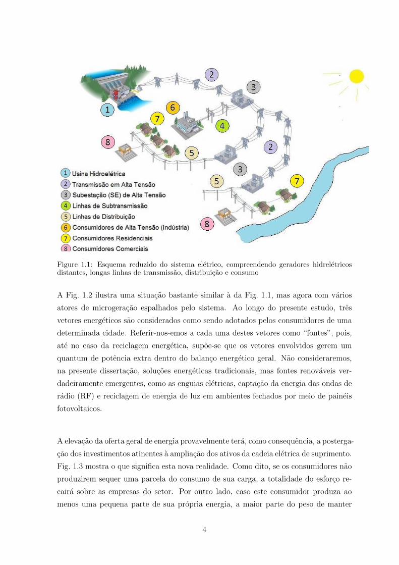
Figure 1.1: Esquema reduzido do sistema eletrico, compreendendo geradores hidreletricosdistantes, longas linhas de transmissao, distribuicao e consumo
A Fig. 1.2 ilustra uma situacao bastante similar a da Fig. 1.1, mas agora com varios
atores de microgeracao espalhados pelo sistema. Ao longo do presente estudo, tres
vetores energeticos sao considerados como sendo adotados pelos consumidores de uma
determinada cidade. Referir-nos-emos a cada uma destes vetores como “fontes”, pois,
ate no caso da reciclagem energetica, supoe-se que os vetores envolvidos gerem um
quantum de potencia extra dentro do balanco energetico geral. Nao consideraremos,
na presente dissertacao, solucoes energeticas tradicionais, mas fontes renovaveis ver-
dadeiramente emergentes, como as enguias eletricas, captacao da energia das ondas de
radio (RF) e reciclagem de energia de luz em ambientes fechados por meio de paineis
fotovoltaicos.
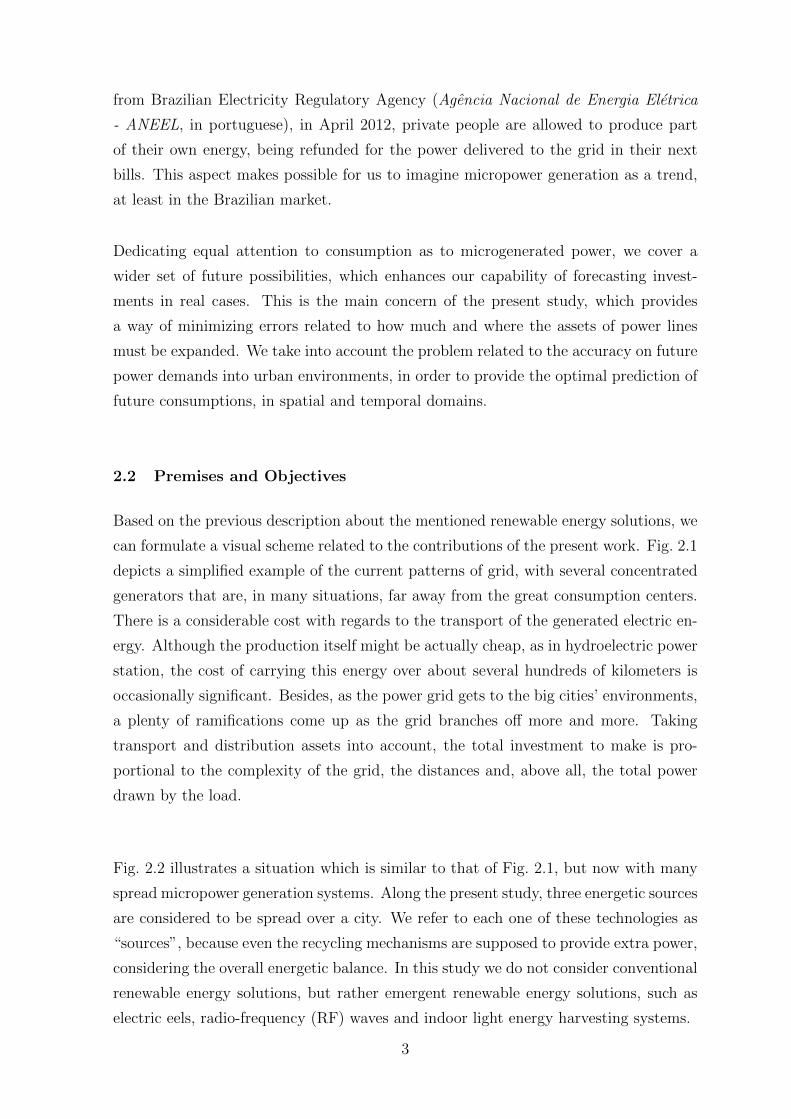
A elevacao da oferta geral de energia provavelmente tera, como consequencia, a posterga-
cao dos investimentos atinentes a ampliacao dos ativos da cadeia eletrica de suprimento.
Fig. 1.3 mostra o que significa esta nova realidade. Como dito, se os consumidores nao
produzirem sequer uma parcela do consumo de sua carga, a totalidade do esforco re-
caira sobre as empresas do setor. Por outro lado, caso este consumidor produza ao
menos uma pequena parte de sua propria energia, a maior parte do peso de manter
4

Figure 1.2: Esquema da Fig. 1.1, agora incluindo enguias eletricas nadando em um rio erecicladores RF sobre as casas, ambos fornecendo energia para o sistema eletrico interligado,enquanto um analisador de dados reune os dados de consumo das Subestacoes envolvidas
Figure 1.3: Comparacao entre as redes com e sem microgeradores distribuıdos: a pessoarepresenta os geradores, a corda e comparada com as linhas de transmissao, um bloco pesadorepresenta a carga, e o contrapeso auxiliar representa a microgeracao: (a) a pessoa efetuao esforco sozinha, e (b) o esforco de sustentar a carga e parcialmente dividido entre ela e ocontrapeso auxiliar.
5

o funcionamento do sistema ainda recai sobre os ativos tradicionais, mas agora este
esforco resta diminuıdo.
A ideia central da reciclagem de energia, assim como a da propria microgeracao dis-
tribuıda, e a de aliviar a rede de alguns investimentos no curto prazo, ao mesmo tempo
em que diminui o risco de insuficiencia do suprimento. Quanto maior o contrapeso
auxiliar na Fig. 1.3(b), menor sera a forca requerida da pessoa puxando a carga; ainda,
a corda suportara com maior seguranca os padroes de tracao, e a polia ficara em
condicoes de girar sem grandes problemas.
As contribuicoes do presente trabalho sao baseadas em prospectar dois topicos princi-
pais: investigacao sobre os efeitos da microgeracao distribuıda a ser inserida por toda
a rede, e a analise da predicao deste consumo em series temporais. Ambos os objetivos
sao agora separadamente descritos.
O primeiro objetivo desta pesquisa esta relacionado com a avaliacao energetica da mi-
crogeracao a ser espalhada pela rede. Duas formas emergentes de reciclagem de energia
sao combinadas com uma nova fonte de energia renovavel. A primeira tecnologia de
reciclagem e relativa ao aproveitamento da energia fotovoltaica da luz em ambientes
fechados, por meio de paineis instalados no interior de edificacoes. O segundo reciclador
de energia aproveita a potencia eletromagnetica das Radio Frequencias (RF) existente
no espaco, com enfase a sua exploracao em ambientes predominantemente urbanos.
Podemos dizer que ambos os tipos consistem em reciclagem de energia proveniente do
espectro electromagnetico - o primeiro reciclando a luz, e o segundo, ondas radio. O
terceiro elemento analisado, que e uma fonte de energia em si e nao um vetor de reci-
clagem, e a enguia eletrica, ou poraque. Este peixe de agua doce e muito observado na
Amazonia brasileira e converte a energia quımica de seu alimento em tensao eletrica
ao longo de seu corpo. Estes tres vetores energeticos sao avaliados tecnicamente, sendo
estimadas as possıveis contribuicoes energeticas de cada uma delas para a rede.
O segundo objetivo desta dissertacao e a analise da predicao de series espaciais-temporais,
que contam com metodos matematicos uteis em predizer valores de series temporais.
Da cidade de Leipzig (Saxonia, Alemanha) obtivemos dados diarios de consumo ao
longo de 4 anos, envolvendo 8 Subestacoes de potencia (SE). A razao de adotar Leipzig
como a cidade de analise neste trabalho foi a disponibilidade de um preciso e coeso
conjunto de dados diarios.
6

Quatro metodos foram testados de forma a tornar possıvel a identificacao do mais ade-
quado para prever a informacao: modelo Auto-Regressivo (AR), Auto-Regressivo com
um elemento eXogeno (ARX), Auto-Regressivo de Medias Moveis com um elemento
eXogeno (ARMAX) e Redes Neurais Artificiais (ANN). Os tres primeiros metodos sao
modelos Box & Jenkins. O elemento exogeno presente nos modelos ARX e ARMAX foi
a temperatura: primeiramente, seu valor real foi adotado, e em seguida foram incluıdos
seus valores logarıtmicos.
Na sequencia, dois principais estagios foram empreendidos, sendo a microgeracao dis-
tribuıda considerada apenas no segundo estagio. Todos estes passos buscaram determi-
nar qual o metodo mais preciso para predicao de valores futuros: AR, ARX, ARMAX
ou ANN.
Previsoes espaciais advieram dos resultados obtidos na predicao temporal, uma vez que
os futuros valores encontrados para a carga no tempo sao aplicados a cada uma das 8
SEs consideradas.
Como o escopo da presente dissertacao tem dois focos diferentes e harmonicos, devemos
descrever os provaveis benefıcios finais deste trabalho. Uma vez que os dados sobre
consumo oriundos de algumas SEs estiverem disponıveis, o processamento de futuros
valores de demandas e uma tarefa possıvel, e ainda com a indicacao de qual metodo
- se ANN, AR, ARX ou ARMAX - e o melhor para tanto. Assume-se que os dados
relativos as potencia demandada estao a disposicao da empresa de distribuicao de
energia eletrica. Uma vez que esta informacao esta ao alcance, valores futuros de
demanda podem ser determinados com razoavel precisao. Os benefıcios relacionados a
predicao dividem-se em duas frentes:
• como exemplo de aplicacao no curto prazo, temos que se a empresa preve para
as proximas semanas uma elevacao em uma das demandas que venha a ofere-
cer qualquer ameaca a continuidade do suprimento, a empresa pode se prevenir
contra este evento agindo sobre os gargalos. Por exemplo, consideremos uma pre-
visao de que em duas semanas um pico de potencia tem uma certa probabilidade
de ocorrencia de tal forma que possa se aproximar dos limites de especificacao de
um dos transformadores. Nesse caso, poderia ser uma solucao ativar um segundo
transformador na respectiva SE em vista dessa previsao especıfica.
• como exemplo de aplicacao no medio prazo, considerando um conjunto de dados
7

mensais ou anuais, se a empresa verifica que, de acordo com a tendencia, um
grupo de transformadores deve suportar potencias que nao podem atender dadas
suas especificacoes, eles tornam-se gargalos do sistema, devendo aı a rede ser
expandida.
No exemplo atinente ao curto prazo, haveria ainda a possibilidade de que o sistema
viesse a pagar uma taxa mais cara pelo Wh adicional gerado pelos consumidores, no
caso de se tratar de uma semana crıtica. Obviamente, tal decisao deve estar amparada
pelas disposicoes regulatorias vigentes.
Dado que serao caracterizados valores plausıveis para as fontes renovaveis em questao
- enguias, RF e reciclagem de luz em ambientes fechados -, ganha-se informacao para
futuros estudos que venham a adota-las.
1.3 Como esta Dissertacao esta Organizada
O Capıtulo 3 inicia o estudo da dissertacao propriamente dita, abordando as tres
fontes renovaveis que serao empregadas: conversao fotovoltaica, reciclagem de ondas
eletromagneticas RF e enguias eletricas. Para cada uma destas fontes, expoe-se a teoria
geral e o que ha no estado da arte. As medicoes da potencia passıvel de ser fornecida
ajuda a moldar os circuitos de gerenciamento da energia aplicaveis.
Tanto no Capıtulo 4 como no 5, um conjunto de dados de demandas de potencia abarca
4 anos (2001-2004), ou 209 semanas. As maximas demandas de potencia semanal
basearam-se em registros pormenorizados de 8 SEs, totalizando 209 dados sequenciados
para cada SE. Os capıtulos 4 e 5 tambem mencionam como se deram as aplicacoes
dos sistemas ANN e Box & Jenkins (AR, ARX and ARMAX) sobre os dados reais
observados. Uma vez que estes capıtulos procedem a calculos relacionados com estes
sistemas, o leitor deve considerar a possibilidade de visitar os Apendices A e B caso
deseje entender ou relembrar a transformada z e as estruturas AR, ARX e ARMAX.
O capıtulo 4 descreve a analise preditiva da carga tal qual os dados foram apanhados das
SEs de Leipzig, isto e, sem que ainda fosse considerada a insercao das fontes emergentes
no sistema eletrico. Para os modelos AR, ARX e ARMAX, a ordem otima do modelo foi
selecionada a partir do criterio da Descricao por Dimensoes Mınimas (DDM). Os valores
de temperatura e seus logaritmos foram analisados como possıvel variavel eXogena (o
8

X de ARMAX). Produzimos, entao, os modelos AR, ARX e ARMAX para as ultimas
9 semanas, e para cada SE. Falando agora das estruturas ANN, de redes neurais, ela
foi treinada ao longo das primeiras 200 semanas, produzindo saıdas para as ultimas 9
semanas de dados do perıodo total de 209 semanas. Assim sendo, em nome de uma
comparacao justa, utilizamos a mesma quantidade de dados de entrada e previmos
a mesma quantidade de informacao, usando tanto estruturas ANN quanto ARMAX.
Todos os modelos foram, entao, comparados uns com os outros segundo a mesma
quantidade de dados.
O Capıtulo 5 insere as fontes renovaveis nas casas, industrias e predios publicos. As
mesmas informacoes de 209 semanas (2001-2004) foram admitidas como dados de en-
trada. Projetamos possıveis valores energeticos oriundos das fontes para diferentes
perıodos ao longo das ultimas 157 semanas, em instantes iniciais aleatorios. Novos val-
ores para demandas maximas semanais foram entao obtidas a partir da diferenca entre
os valores reais medidos e os valores calculados para cada fonte renovavel. Esses novos
conjuntos de valores foram, assim, adotados como o novo rol de dados de entrada. Posto
que durante 2001 ainda nao havia energia proveniente das fontes emergentes, mas ape-
nas durante o perıodo 2002-2004, e considerando que as fontes renovaveis entram com
energia na rede progressivamente, foram simuladas novas tendencias para as maximas
demandas de potencia tal como enxergadas pelas SEs. Em seguida, nos treinamos a
malha ANN e ajustamos os modelos AR, ARX e ARMAX de acordo com as primeiras
200 semanas. Avaliamos, entao, a habilidade de adaptacao de cada metodo no sentido
de predizer os consumos semanais para as ultimas 9 semanas de 2004.
A existencia de microgeracao distribuıda nao e informada para a empresa de dis-
tribuicao, nas aplicacoes dos modelos ANN, AR, ARX e ARMAX; a empresa deve
apenas detectar as novas tendencias da carga e adaptar-se a elas.
Tanto no capıtulo 4 como no 5, foi estabelecido que a rede neural conta com duas
camadas escondidas. Nossos codigos MATLAB detectaram o melhor numero possıvel
para cada camada escondida. Portanto, as previsoes via ANN foram obtidas com essa
quantidade otima de neuronios por camada.
O Capıtulo 6 contem consideracoes sobre o experimento em geral e oferece uma con-
clusao objetiva com relacao a qual metodo foi o de melhor desempenho para cada um
dos experimentos.
9

Ha, ainda, dois apendices com um util arcabouco teorico que ampara varias decisoes
tomadas ao longo desta dissertacao. O Apendice A revisa Series Estacionarias e discute
conceitos atinentes a estacionariedade de series temporais, que sao requisitos para os
filtros lineares utilizados nos Capıtulos 3 e 4. O Apendice B contem a Transformada
Z, compreendendo modelos auto-regressivos (AR), de media movel (MA), ARX (AR
com variavel exogena) e ARMAX. Por fim, o Apendice C elenca varios resultados de
predicao espacial no que tange a reducao percentual da carga no horario de ponta para
os bairros em que se situam as Subestacoes de Potencia. Alguns destes resultados sao
mostrados no final do Capıtulo 5; porem, em face da imensa quantidade de exemplos
possıveis a partir da variacao de alguns parametros de crescimento das fontes, um
Apendice especıfico foi idealizado.
10
Chapter 2 INTRODUCTION
2.1 Motivation
Electric energy is not only intimately related to human development, richness and
comfort; it can be understood as the basis of such concepts, even because it is as such
considered in the realm of economic analyzes. Human life was radically modified by
the advent of electricity, and it is no longer possible to live in a satisfying way without
it.
All over the world, large parts of energy supply are set apart to industry and transport,
which are in many economies the most energetic intensive sectors. That is a simple and
effective explication why the richest countries have the highest energetic demands per
inhabitant. According to [1], the 30 developed countries which integrate the OECD are
historically the greatest energy consumers. In addition to it, growing-rates for GDP
are intrinsically energetic data: in [2], it is pointed out an almost linear relationship
between the worldwide increasing energetic demand and GDP growth, considered the
years from 2003 to 2007. Energetic intensity, the indicator which establishes how much
energy is necessary to produce GDP, is higher in countries which have larger portions
of population with access to energetic intensive consumer goods [3].
Despite the modern and questionable theories about the new relationship between
energy and economic development, all these evidences show the undeniable connection
between wealth and energy consumption. According to [4], in Brazil, electricity stands
for 17 % of the final energy consumption in 2012. The same document states, for the
year 2012, the evolution of some indicators of Brazilian economy over the period 2003-
2012: during these 10 years, Domestic Energy Supply (DES), Gross Domestic Product
(GDP) and population in millions of inhabitants have evolved as shown in Table 2.1:
In Table 2.1, toe stands for ton oil equivalent, energy unit equivalent to 11.63 MWh.
The energy supply for internal inhabitants usually increases despite of the growing
population, and, moreover, the DES keeps very pace with GDP evolution. Due to the
worldwide economic crisis which has had its climax in 2008, carrying forth consequences
for the GDP rates all over the globe, GDP and DES for 2009 were below the expected
1

Table 2.1: Domestric Energy Supply (DES), Gross Domestic Product (GDP) and Populationfrom 2003 to 2012 in Brazil [4]
Unit 2003 2004 2005 2006 2007 2008 2009 2010 2011 2012
DES 106 toe 201.9 213.4 218.7 226.3 237.8 252.6 243.9 268.8 272.3 283.6
GDP 109 US$ 1426.1 1507.5 1555.2 1616.7 1715.2 1803.9 1797.9 1933.4 1986.2 2003.5
Population 106 inhab 176.6 178.7 180.8 182.9 185.0 187.2 189.4 191.6 193.2 194.7
DES/GDP toe/103 US$ 0.142 0.142 0.141 0.140 0.139 0.140 0.136 0.139 0.137 0.142
DES/capita toe/inhab 1.143 1.194 1.210 1.238 1.285 1.350 1.288 1.403 1.410 1.457
trend. Despite of that, DES/GDP remained approximately constant all over the years,
even with the perturbation arised by the economy, as it is demonstrated in this decade,
since the amplitude of maximum variation barely overcame 4% of the mean 0.140. This
confirms the very known principle by which economic development is deeply related to
the increase of energy offer.
As electric energy is one the main forms of energy, electricity and the overall energy
supply are supposed to arise or come down together. Furthermore, since economic
benefits are expected only when energy offer goes up, electricity must do the same.
Therefore, the need related to understanding electricity management comes up as a
crucial subject, in Economy as much as in Engineering.
In order to be consumed, electricity must be generated, transformed and transported
over wide distances, which are specially wide in cases as the Brazilian, whose centers of
generation are very far away from those of consumption. It consists on a form of energy
much sensitive to infrastructure. The amount of electrical power transmission lines
can transport over kilometers is fundamentally dependent on its physical parameters,
like transformers properties, for instance. Since distribution power lines even into
urban environments represent huge infrastructure investments, errors or improprieties
in planning such assets expansion may breed economic losses for years. This need
of keeping available power always above instantaneous consumption justifies electric
power microgeneration as an advantageous measure, due to the incremental power offer
to the overall balance, as discussed in Section 1.2 and demonstrated in Chapter 4. In
many situations, microgenerators enable the load to assume a flatter behavior, i. e.,
with less variance on power demand values, given that microgenerators can sustain
part of the load in the daily peak, when the value of unitary kWh is more expensive.
Furthermore, power microgenerators count nowadays on a favorable environment to
prosper within countries in which consumers are allowed to furnish to the grid the
surplus of their power generation. In Brazil, since the edition of the Resolution no 482
2
from Brazilian Electricity Regulatory Agency (Agencia Nacional de Energia Eletrica
- ANEEL, in portuguese), in April 2012, private people are allowed to produce part
of their own energy, being refunded for the power delivered to the grid in their next
bills. This aspect makes possible for us to imagine micropower generation as a trend,
at least in the Brazilian market.
Dedicating equal attention to consumption as to microgenerated power, we cover a
wider set of future possibilities, which enhances our capability of forecasting invest-
ments in real cases. This is the main concern of the present study, which provides
a way of minimizing errors related to how much and where the assets of power lines
must be expanded. We take into account the problem related to the accuracy on future
power demands into urban environments, in order to provide the optimal prediction of
future consumptions, in spatial and temporal domains.
2.2 Premises and Objectives
Based on the previous description about the mentioned renewable energy solutions, we
can formulate a visual scheme related to the contributions of the present work. Fig. 2.1
depicts a simplified example of the current patterns of grid, with several concentrated
generators that are, in many situations, far away from the great consumption centers.
There is a considerable cost with regards to the transport of the generated electric en-
ergy. Although the production itself might be actually cheap, as in hydroelectric power
station, the cost of carrying this energy over about several hundreds of kilometers is
occasionally significant. Besides, as the power grid gets to the big cities’ environments,
a plenty of ramifications come up as the grid branches off more and more. Taking
transport and distribution assets into account, the total investment to make is pro-
portional to the complexity of the grid, the distances and, above all, the total power
drawn by the load.
Fig. 2.2 illustrates a situation which is similar to that of Fig. 2.1, but now with many
spread micropower generation systems. Along the present study, three energetic sources
are considered to be spread over a city. We refer to each one of these technologies as
“sources”, because even the recycling mechanisms are supposed to provide extra power,
considering the overall energetic balance. In this study we do not consider conventional
renewable energy solutions, but rather emergent renewable energy solutions, such as
electric eels, radio-frequency (RF) waves and indoor light energy harvesting systems.
3

Figure 2.1: Reduced scheme of the electric system, comprehending far away hydro-generators,long transmission lines, distribution and consumption.
The enhancement of the overall generation probably will have, as a consequence, the
postponement of investments concerning to the enlargement of the assets of electric
supply chains. Fig. 2.3 illustrates what would be this new reality. As said, whether
consumers do not produce even a fraction of their electric load, the totality of the effort
falls on the public utility. On the other hand, if this consumer produces at least a little
part of their own energy, the bulk of the energetic burden continues to lie with the
utility, but this effort is now shortened a little.
The core idea of recycling energy, as well as that of the distributed microgeneration,
is to relieve the grid from investments in the short-term, simultaneously diminishing
the risk of supply insufficiency. The higher is the auxiliary weight within Fig. 2.2(b),
the softer will be the force which is required from the man; furthermore, the rope has
a greater assurance in supporting the traction, as well as the pulley is more likely to
roll without problems.
The contributions of the present work are based on the probing of two main topics:
investigation about the effects of the micropower generation to be inserted all over
4
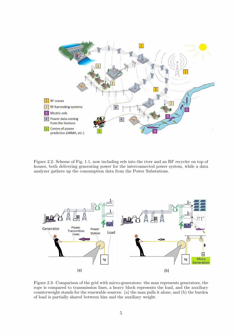
Figure 2.2: Scheme of Fig. 1.1, now including eels into the river and an RF recycler on top ofhouses, both delivering generating power for the interconnected power system, while a dataanalyzer gathers up the consumption data from the Power Substations.
Figure 2.3: Comparison of the grid with micro-generators: the man represents generators, therope is compared to transmission lines, a heavy block represents the load, and the auxiliarycounterweight stands for the renewable sources: (a) the man pulls it alone, and (b) the burdenof load is partially shared between him and the auxiliary weight.
5

the grid, and spatio-temporal series predicition analysis. Both objects are hereafter
separately described.
The first goal of this research is related to the energetic evaluation of micropower
generation to be inserted all over the grid. Two emergent forms of recycling energy
are combined to a novel renewable source. The first recycling technology is energy
haversting from indoor light, by means of solar panels installed within buildings. The
second energy recycler manages the eletromagnetic power from Radio Frequency (RF),
which is spread all over the space, with emphasis to urban environments. We can
say that both types consist on recycling energy of electromagnetic spectrum, the first
one recycling light and the second one recycling radio frequencies. The third analyzed
element, which is an energy source itself rather than a recycling scheme, is the electric
eel. This freshwater fish is rife in Brazilian Amazonia and converts chemical energy
existing in their food into voltage along their body. All these three vectors are techni-
cally analyzed, and we assess the possible energetic contribution from each one to the
grid.
The second goal of this dissertation is the spatio-temporal series analysis, which relies
on useful mathematical methods to predict values of time series. The city of Leipzig
(Saxon, Germany) has furnished its electrical data over 4 years involving 8 Power
Substations (PS). The reason for adopting Leipzig as our city in this study was the
availability of such set of data in details.
Four methods were tested in order to make it possible identifying the more suitable
one to forecasting information: Auto-Regressive (AR) Model, Auto-Regressive with an
eXogeneous Input (ARX), Auto-Regressive Moving Average with ans eXogeneous Input
(ARMAX) and Artificial Neural Networks (ANN). The three first methods are Box &
Jenkins Models. The eXogeneous input within ARX and ARMAX was temperature:
priorly, its real measured value was adopted, and then we handled its logarithmic
values.
In sequel, two main stages were undertaken, microgeneration being considered only in
the second stage. All these tasks were developed in order to determine the more precise
method: AR, ARX, ARMAX or ANN.
Spatial forecasts arose from the temporal results, since the future values of load in time
are applied to each one of the 8 considered PS.
6

As the scope of this work has two different and harmonic focuses, we should describe
the benefits of such study in the way it is idealized. Since many data about electrical
consumption of a set of Power Substations is available, the processing of the future
values is possible, even with the indication of which method - if ANN or ARMAX -
is the best one for that. We take for grant that demand power data are within the
reach of the electric distribution utility. Once this information is available, futures
values of demand are determined with resonable precision. The benefits with respect
to prediction comprise two fronts:
• as an example of application in the short-term, if the utility forecast any raise
within future power demands, which might offer any threat to the assurance of
supply, the utility can prevent such issue, acting upon bottlenecks. For instance,
consider a forecast which informs us that two weeks from now a maximum value is
likely to occur in such a way that it may approach the boundaries of transformer
capacity. In this case, it might be a solution to turn on an existing second
transformer in the Power Substation for this specific event.
• as an example of application in the mean-term, considering therefore a monthly
or annual set of data, if the utility finds out that an increasing number of trans-
formers are about to face power demands that they would not support given
their specifications, these transformers become bottlenecks, and therefore the
grid must be expanded.
In the short-term example, there is still the possibility of paying some more for each
additional Wh generated by the consumers, whether the present week is a critical one.
Obviously, such decision should be supported by the regulatory laws.
Since we are going to feature realistic values for the mentioned renewable sources -
eels, RF and indoor light harvesting systems -, there is a gain of information for future
studies which intend to adopt these energetic sources.
2.3 How this Dissertation is Organized
Chapter 3 initiates the proper study existing in the present dissertation, approaching
the three renewable sources which will be employed: photovoltaic conversion, electro-
magnetic waves recycling. For each source, we approach the theory and the state of
7
the art. Measurements of deliverable power helps to determine the specifications for
the applicable management circuits.
In both chapters 4 and 5, the set of power demands covers 4 years (2001-2004), or
209 weeks. Weekly maximum power demand data counted on 8 PSs detailed demand
registers, performing 209 sequenced data for each PS. Chapters 4 and 5 also cover the
application of ANN and Box & Jenkins (AR, ARX and ARMAX) models upon real
recorded data. Since these chapters carry out calculations related only to these models,
the reader must consider take a look at the Appendices A and B in order to review
z-transform and ARMAX concepts, respectively.
Chapter 4 describes the predictive analysis of the load as they were extracted from
Leipzig Power Substations, i. e., with no emergent power microgenerators being con-
sidered. For the AR, ARX and ARMAX models, the optimal order of parameters were
selected via Minimum Description Length (MDL) criterion. Temperature values and
their logarithm were analyzed as a possible eXogeneous variable, therefore ARMAX
with X at the end. We have then produced AR, ARX and ARMAX models for the last
9 weeks, and for each PS. Talking now about ANN structure, we trained it over the
first 200 weeks, returning outputs for the last 9 weeks of data from the entire period
of 209 weeks. Therefore, in order to perform a fair comparison, we utilized the same
quantity of input data and forecasted the same amount of information, either making
use of ANN and ARMAX models. All models were then compared each other counting
on the same set of data.
Chapter 5 inserts the renewable sources into houses, industries and public buildings.
The same 209 weeks data (2001-2004) were admitted as input data. We projected
possible energetic values from the sources for different periods into the last 157 weeks,
in random initial instants. New values for maximum power demands are then obtained
from the difference between the realistic values and those coming from the renewable
sources. These new sets of values have thus been adopted as our set of input data.
Since during 2001 there is not yet input from renewables, but only during the 2002-
2004 period, and given that these renewable sources enter in the grid progressively,
we simulated a new trend for the power demand values seen by the PS. In the sequel,
we trained our ANN and adjusted our AR, ARX and ARMAX models according to
the first 200 weeks. We have then evaluated the adaptation ability of each method to
forecast the weeks demands for the 9 last weeks of 2004.
8

The existence of power microgeneration is not informed to the grid in ANN, AR, ARX
and ARMAX applications; the energy utility has the mission of only detecting the new
trend for power demands, and adapting itself to the new curves.
In both chapters 4 and 5, we established that our ANN system has two hidden lay-
ers. We have exhaustively searched for the number of neurons which gives the best
performance. Therefore, ANN forecasts were obtained with these optimal quantity of
neurons per layer.
Chapter 6 contains considerations about the overall experiment and accomplishes an
objective conclusion with respect to the best model achieved for each one of the exper-
iments.
There are still two appendices with useful concepts that support the proposals all over
this dissertation. Appendix A goes over Stationary Series and discusses concepts about
temporal series stationarity, which are requisites for the linear filters used in Chapters
3 and 4. Appendix B contains Z-Transform concepts, comprising auto-regressive (AR)
model, moving average (MA) model, ARX (AR with eXogeneous variable) and AR-
MAX. Finally, Appendix C gathers several results of spatial prediction of percent peak
load reductions for the districts in which the Power Substations lie. Some results are
initially shown in the final part of Chapter 5; however, given the huge quantity of
possible examples which consider the source parameters variation, a specific Appendix
was idealized.
9
Chapter 3 EMERGENT RENEWABLE SOURCES
In this chapter we examine three sources of electric energy, which are divided into
two energy recyclers, which are the Radio Frequency (RF) energy harvesting and the
indoor light energy harvesting, and an energetic source itself, which is the electric eel.
From now on, despite of the fact that we are dealing with one source and two recycling
forms, all the three energy vectors are going to be treated as “renewable sources”. For
each one of them, the theory and state of the art are overviewed, and data which result
from measurements are exposed.
3.1 RF Energy Harvesting
3.1.1 Theory and State of the Art
The main objective of the RF energy harvesting system is to convert the RF power from
the space into usable direct current (DC) electrical source [5, 6]. In order to achieve
that, a system with several stages is required. The first element is the RF source,
which is the TV and Radio broadcast transmitters in our cities. The next necessary
element is our RF receiver with its matching circuit. While specifying it, one must pay
heed to the exploited band, since the manegement circuit is placed at the input stage
to equalize the impedance between the antenna and the next component of the circuit.
Next, the voltage booster and the rectifier are the items of our highest concern, since
our circuit for energy management may constitute a point of power losses. Finally, the
energy storage system, which is a battery. Fig 3.1 shows the sequence of elements as
here described.
If one antenna serves to furnish power specifically to another antenna, it embodies a
dedicated system, which does not apply to the energy harvesting definition [7]. Recy-
cling power occurs when the energetic proposal of the source does not correspond to its
original utilization. For instance, we suppose an antenna to broadcast eletromagnetic
signal all over the space. In doing so, a certain part of the antenna irradiation can be
absorbed by any device, like antennas which aim to scavenge the energy from the wave,
while ignoring the signal which is conveyed by the transmitter. But an antenna itself
10
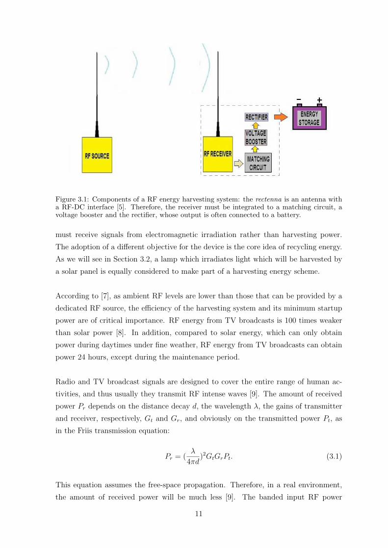
Figure 3.1: Components of a RF energy harvesting system: the rectenna is an antenna witha RF-DC interface [5]. Therefore, the receiver must be integrated to a matching circuit, avoltage booster and the rectifier, whose output is often connected to a battery.
must receive signals from electromagnetic irradiation rather than harvesting power.
The adoption of a different objective for the device is the core idea of recycling energy.
As we will see in Section 3.2, a lamp which irradiates light which will be harvested by
a solar panel is equally considered to make part of a harvesting energy scheme.
According to [7], as ambient RF levels are lower than those that can be provided by a
dedicated RF source, the efficiency of the harvesting system and its minimum startup
power are of critical importance. RF energy from TV broadcasts is 100 times weaker
than solar power [8]. In addition, compared to solar energy, which can only obtain
power during daytimes under fine weather, RF energy from TV broadcasts can obtain
power 24 hours, except during the maintenance period.
Radio and TV broadcast signals are designed to cover the entire range of human ac-
tivities, and thus usually they transmit RF intense waves [9]. The amount of received
power Pr depends on the distance decay d, the wavelength λ, the gains of transmitter
and receiver, respectively, Gt and Gr, and obviously on the transmitted power Pt, as
in the Friis transmission equation:
Pr = (λ
4πd)2GtGrPt. (3.1)
This equation assumes the free-space propagation. Therefore, in a real environment,
the amount of received power will be much less [9]. The banded input RF power
11
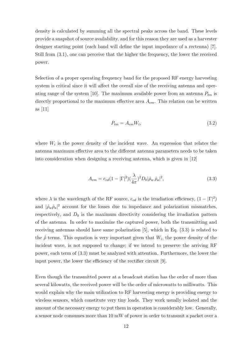
density is calculated by summing all the spectral peaks across the band. These levels
provide a snapshot of source availability, and for this reason they are used as a harvester
designer starting point (each band will define the input impedance of a rectenna) [7].
Still from (3.1), one can perceive that the higher the frequency, the lower the received
power.
Selection of a proper operating frequency band for the proposed RF energy harvesting
system is critical since it will affect the overall size of the receiving antenna and oper-
ating range of the system [10]. The maximum available power from an antenna Ptm is
directly proportional to the maximum effective area Aem. This relation can be written
as [11]
Ptm = AemWi, (3.2)
where Wi is the power density of the incident wave. An expression that relates the
antenna maximum effective area to the different antenna parameters needs to be taken
into consideration when designing a receiving antenna, which is given in [12]
Aem = ecd(1− |Γ|2)(λ
4π)2D0|ρw ρa|2, (3.3)
where λ is the wavelength of the RF source, ecd is the irradiation efficiency, (1− |Γ|2)and |ρwρa|2 account for the losses due to impedance and polarization mismatches,
respectively, and D0 is the maximum directivity considering the irradiation pattern
of the antenna. In order to maximize the captured power, both the transmitting and
receiving antennas should have same polarization [5], which in Eq. (3.3) is related to
the ρ terms. This equation is very important given that Wi, the power density of the
incident wave, is not supposed to change; if we intend to preserve the arriving RF
power, each term of (3.3) must be analyzed with attention. Furthermore, the lower the
input power, the lower the efficiency of the rectifier circuit [9].
Even though the transmitted power at a broadcast station has the order of more than
several kilowatts, the received power will be the order of microwatts to milliwatts. This
would explain why the main utilization to RF harvesting energy is providing energy to
wireless sensors, which constitute very tiny loads. They work usually isolated and the
amount of the necessary energy to put them in operation is considerably low. Generally,
a sensor node consumes more than 10 mW of power in order to transmit a packet over a
12
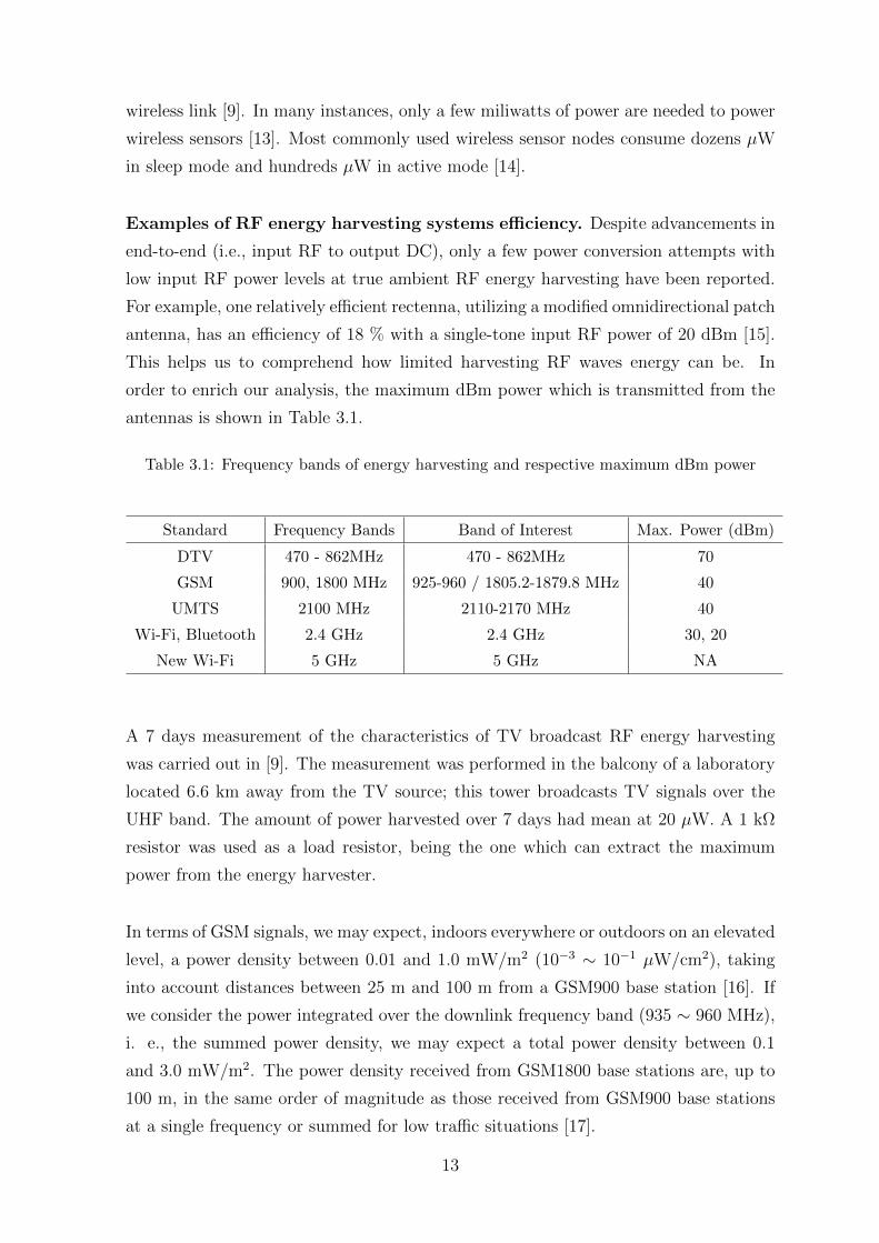
wireless link [9]. In many instances, only a few miliwatts of power are needed to power
wireless sensors [13]. Most commonly used wireless sensor nodes consume dozens µW
in sleep mode and hundreds µW in active mode [14].
Examples of RF energy harvesting systems efficiency. Despite advancements in
end-to-end (i.e., input RF to output DC), only a few power conversion attempts with
low input RF power levels at true ambient RF energy harvesting have been reported.
For example, one relatively efficient rectenna, utilizing a modified omnidirectional patch
antenna, has an efficiency of 18 % with a single-tone input RF power of 20 dBm [15].
This helps us to comprehend how limited harvesting RF waves energy can be. In
order to enrich our analysis, the maximum dBm power which is transmitted from the
antennas is shown in Table 3.1.
Table 3.1: Frequency bands of energy harvesting and respective maximum dBm power
Standard Frequency Bands Band of Interest Max. Power (dBm)
DTV 470 - 862MHz 470 - 862MHz 70
GSM 900, 1800 MHz 925-960 / 1805.2-1879.8 MHz 40
UMTS 2100 MHz 2110-2170 MHz 40
Wi-Fi, Bluetooth 2.4 GHz 2.4 GHz 30, 20
New Wi-Fi 5 GHz 5 GHz NA
A 7 days measurement of the characteristics of TV broadcast RF energy harvesting
was carried out in [9]. The measurement was performed in the balcony of a laboratory
located 6.6 km away from the TV source; this tower broadcasts TV signals over the
UHF band. The amount of power harvested over 7 days had mean at 20 µW. A 1 kΩ
resistor was used as a load resistor, being the one which can extract the maximum
power from the energy harvester.
In terms of GSM signals, we may expect, indoors everywhere or outdoors on an elevated
level, a power density between 0.01 and 1.0 mW/m2 (10−3 ∼ 10−1 µW/cm2), taking
into account distances between 25 m and 100 m from a GSM900 base station [16]. If
we consider the power integrated over the downlink frequency band (935 ∼ 960 MHz),
i. e., the summed power density, we may expect a total power density between 0.1
and 3.0 mW/m2. The power density received from GSM1800 base stations are, up to
100 m, in the same order of magnitude as those received from GSM900 base stations
at a single frequency or summed for low traffic situations [17].
13
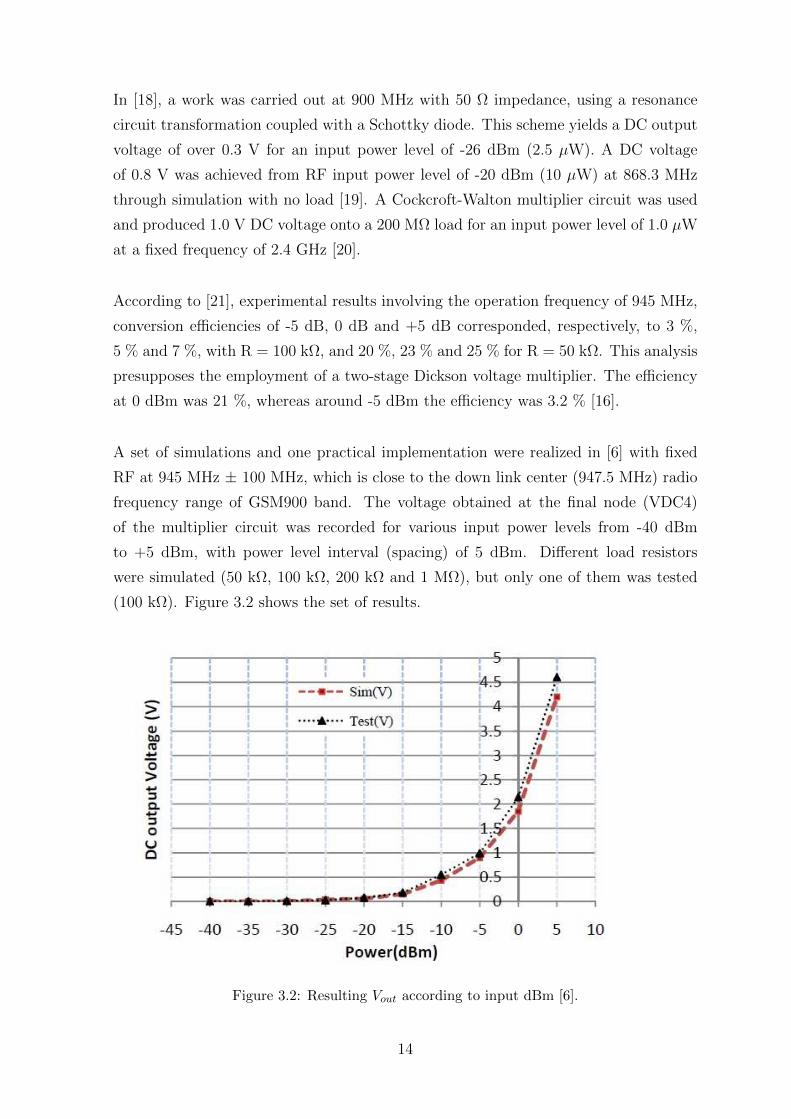
In [18], a work was carried out at 900 MHz with 50 Ω impedance, using a resonance
circuit transformation coupled with a Schottky diode. This scheme yields a DC output
voltage of over 0.3 V for an input power level of -26 dBm (2.5 µW). A DC voltage
of 0.8 V was achieved from RF input power level of -20 dBm (10 µW) at 868.3 MHz
through simulation with no load [19]. A Cockcroft-Walton multiplier circuit was used
and produced 1.0 V DC voltage onto a 200 MΩ load for an input power level of 1.0 µW
at a fixed frequency of 2.4 GHz [20].
According to [21], experimental results involving the operation frequency of 945 MHz,
conversion efficiencies of -5 dB, 0 dB and +5 dB corresponded, respectively, to 3 %,
5 % and 7 %, with R = 100 kΩ, and 20 %, 23 % and 25 % for R = 50 kΩ. This analysis
presupposes the employment of a two-stage Dickson voltage multiplier. The efficiency
at 0 dBm was 21 %, whereas around -5 dBm the efficiency was 3.2 % [16].
A set of simulations and one practical implementation were realized in [6] with fixed
RF at 945 MHz ± 100 MHz, which is close to the down link center (947.5 MHz) radio
frequency range of GSM900 band. The voltage obtained at the final node (VDC4)
of the multiplier circuit was recorded for various input power levels from -40 dBm
to +5 dBm, with power level interval (spacing) of 5 dBm. Different load resistors
were simulated (50 kΩ, 100 kΩ, 200 kΩ and 1 MΩ), but only one of them was tested
(100 kΩ). Figure 3.2 shows the set of results.
Figure 3.2: Resulting Vout according to input dBm [6].
14

There is still an example of incident power in high buildings from [7]. Measurements
within the Department of Electrical and Electronic Engineering building at Imperial
College of London were taken on the 11th floor of the south stairwell. These are shown
in Fig. 3.3. One must note that it is related to the end-to-end efficiency, which is the
quocient between the time-averaged output (i.e., equivalent DC) power into the storage
element and the time-averaged input RF power; in other terms, it depends strongly on
the efficiency of the harvesting system as shown in Fig. 3.1, but also are relevant as
examples for the end-to-end efficiency.
Figure 3.3: End-to-end efficiencies for ambient RF energy harvesting [7].
3.1.2 Measurements
In May 11th 2013, several measurements were undertaken with the aim of evaluating
the use of RF waves as an ubiquitous energy source. Values of incident power, in dBm,
were measured from four points of Brasilia-DF (Brazil) with the aid of a spectrum
analyzer. The measurements were all carried out approximately 1.7 meter above the
soil.
The four surveyed points stay near two main targets of research: the Digital Tower
(1541’57.67”S/4749’46.47”O)1 and the TV Tower (1547’25.49”S / 4753’29.45”O).
For each target, two sites were chosen to verify the incident power in dBm values. The
sites selected to take measurements from the Digital Tower were Place 1 (1541’29.70”S/
1All places here described had their coordinates drawn from Google Earth.
15

4751’13.96”O), on the border of the road leading to the Digital Tower, and Place 2
(1541’59.46”S/4749’50.38”O), right in front of this target. In order to take mea-
surements over RF power irradiance arriving on points around the TV Tower, places
3 (1547’25.13”S/4753’28.88”O) and 4 (1547’39.61”S/4753’11.72”O) were chosen.
These places are depicted in Fig. 3.4.
Figure 3.4: Map of Brasilia-DF (Brazil) with the indicated 4 places on which RF spectrumintensities were measured.
Each one of the four places was visited three time during that day, in order to register
morning, afternoon and evening dBm values. The dBm power level took into account
the corresponding frequency, and therefore several measurements over different fre-
quencies were made so that we could feature the dBm behavior according to the part
of RF spectrum. The graphs made for each place, as shown in Fig. 3.5, comprised
values over an entire day.
16
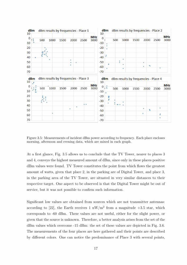
Figure 3.5: Measurements of incident dBm power according to frequency. Each place enclosesmorning, afternoon and evening data, which are mixed in each graph.
At a first glance, Fig. 3.5 allows us to conclude that the TV Tower, nearer to places 3
and 4, conveys the highest measured amount of dBm, since only in these places positive
dBm values were found. TV Tower constitutes the point from which flows the greatest
amount of watts, given that place 2, in the parking are of Digital Tower, and place 3,
in the parking area of the TV Tower, are situated in very similar distances to their
respective target. One aspect to be observed is that the Digital Tower might be out of
service, but it was not possible to confirm such information.
Significant low values are obtained from sources which are not transmitter antennas:
according to [22], the Earth receives 1 nW/m2 from a magnitude +3.5 star, which
corresponds to -60 dBm. These values are not useful, either for the slight power, or
given that the source is unknown. Therefore, a better analysis arises from the set of the
dBm values which overcome -15 dBm: the set of these values are depicted in Fig. 3.6.
The measurements of the four places are here gathered and their points are described
by different colors. One can notice the predominance of Place 3 with several points,
17

whereas Place 2 has just one point in this set of data.
Figure 3.6: Results which overcome -15 dBm, here called “best results”, with values properlysignalized in order to show participation of each place in this group.
The most concentrated part of the spectrum graph stood around 90 MHz. In Fig. 3.6,
all measurement points with regards to places 1 and 4 caught signals around 90 MHz,
as well as the only value of Place 2 which shows up here. Place 3 bears points here
and in the other parts of the graph. The main conclusion is, since we intend to avail
ourselves of the incident RF power, the range of frequency 90-100 MHz is the most
indicated interval to achieve an efficient energy harvesting scheme. All observed places
have relatively good dBm values into 90-100 MHz, and the best dBm values are also
in this range. Therefore, the higher probability of success involves this range.
There are 24 points appearing in this graph, three being in overlap. From the 24 points,
9 were taken in the morning, 8 were taken in the afternoon, and 7 were recorded in the
evening. Accounting on this observation, we assume that the period of the day is not
relevant for obtaining higher or lower values of dBm. The distance to the target and
the target itself are considered much more important.
3.1.3 Expected results given the measurements
We now call upon the known expression shown in (3.4):
dBm = 10 log10
(P
1 mW
)(3.4)
18

This expression provides a rapid way to calculate the incident power as a function of
the measured dBm. Table 3.2 contains a brief set of examples of values which come
from the simple application of (3.4).
Table 3.2: Incident power as a function of dBm values - examples
dBm -15 -10 -6 -3 0 1 2 3 5
Power (mW) 0.032 0.100 0.251 0.501 1.000 1.259 1.585 1.995 3.162
Crossing the average efficiency of 17 % [15] with an incident power of -3 dBm, which
is near to the mean over the graph shown in Fig. 3.6, we achieve the average power of
86 µW. During 24 hours, the total energy harvested achieves 2.058 mWh. This amount
of daily power will be multiplied for the number of antennas, resulting on the daily
available energy for the complete group of RF harvester antennas.
3.2 Indoor Light Energy Recycling
3.2.1 Theory and State of the Art
There are many sources of energy that are not, or barely, used for power generation.
According to [8] and [23], technical aspects enable luminous energy to be one of the
most promising power sources, given that their power density related to area or volume
is among the highest ones. In a outdoor environment, at noon, the ratio of available
energy for a solar cell reaches 15 mW/cm2.
On the other hand, a small piezoelectric generator using shoes movements achieves
330 µW/cm3; a thermoelectric generator (10 C gradient) produces about 40 µW/cm3;
acoustic noise generator (100 dB) falls short of 1 µW/cm3 [23].
We evaluate if luminous energy from artificial light constitutes a potentially exploitable
source in terms of harvesting systems. According to [24], the harvesting involving
indoor environment provides 3 orders of magnitude lower than outdoor environment.
In recent publications [24], [25], [26], [27], [28], [29], [30], [31], [32] there has been
an increasing interest in energy harvesting in indoor environments. However, in [25],
[26], [27], [28], [32], [33], [34], [35], the goal was supplying a sensor node. Due to
the importance of charging portable electronic devices, in this section, we perform
measurements in order to verify the possibility of supplying the battery of a cell phone
19

using artificial light. As an additional contribution, we also propose a circuit to charge
a cell phone using artificial light and we show the efficiency of our proposed circuit by
means of simulations.
In [24], photovoltaic devices are classically optimized for the solar spectrum. Energy-
efficient fluorescent and LED lighting have largely replaced incandescent light bulbs,
so that the spectral profile of artificial light has changed from broad spectra, origi-
nated by low temperature blackbodies, to sharply peaked narrow spectra. Table 3.3
presents a comparison between crystalline Silicon (c-Si), amorphous Silicon (a-Si) and
P3HT/PCBM bulk heterojunctions organic PV (OPV) panels in experiments with light
from solar light, Compact Fluorescent Lamp (CFL), Cold-Cathode Fluorescent Lamp
(CCFL) and LED [24]. Based on Table I, an a-Si solar panel is more suitable for indoor
artificial light in comparison with other types of panels.
Table 3.3: Maximal Efficiency Values for Crystalline Silicon, Amorphous Silicon, and OrganicBHJ Solar Cells under different spectral illumination [24].
crystalline-Si
PV Material amorphous-Si
OPV
Luminous
Solar CFL
49 % 50 %
37 % 74 %
28 % 63 %
Source
CCFL LED
52 % 54 %
70 % 80 %
59 % 63 %
In [27], an amorphous silicon photovoltaic cell (PV) has a relatively high efficiency
at low light intensity levels compared to other types of cells. Such property makes
them particularly suitable for indoor and low power light environments. Other types
of panel, as c-Si, have higher performance in an outdoor environment compared to the
indoor environments due to the scarce spectrum of the artificial light as exemplified in
Fig. 3.7 [24].
3.2.2 Open Circuit and Short Circuit Measurements in Indoor Environ-
ments for the a-Si Panel
Measurements were performed with the a-Si solar panel with no load connected to
it. Our goal here is to observe only the behavior of the a-Si solar panel using indoor
artificial light.
20

400 600 800 1000 1200 1400Wavelength (nm)
Inte
nsity
Fluorescent light spectrum
Solar light spectrum
Figure 3.7: Typical solar light AM 1.5 and cold-cathode fluorescent light spectra.
Given that incandescent light bulbs are falling into disuse in many countries, in this
Section only fluorescent and LED lamps are considered. This factor is determinant for
choosing a-Si panel, since it offers a higher efficiency to produce power from such spec-
trum as shown in the previous section. Another reason to choose a-Si panel lies on its
low cost. From now on, all presented results were obtained by means of measurements
obtained in our laboratory.
A panel of amorphous Silicon (a-Si) with maximum current Imax = 200 mA and max-
imum voltage Vmax = 6 V and with size of 95 mm x 110 mm is employed in the
experiments. Over 54 measurements were performed with the a-Si panel being under
different light intensity levels. The variables of interest are open circuit voltage, Voc,
and short circuit current, Isc, in function of incident lux Lx. A white 8 W LED light
bulb (color temperature 4.700 K) was used for the measurements. Figures 3.8 and 3.9
show the curves obtained during the measurements. Intensity and spectrum of light
were kept constant, whereas distance between panel and LED was varied, in order to
provide several light intensity levels.
From the curves of Figs. 3.8 and 3.9, Eqs. (3.5) and (3.6) can be written with the
relationship between Voc and Lx and between Isc and Lx:
Voc = −0.68789 + 0.68159 · ln(Lx), (3.5)
Isc = 0.00074 + 0.00084Lx, (3.6)
where ln(·) is the natural logarithm operator.
21

0 500 1000 1500 2000Lux
1.5
2.0
2.5
3.0
3.5
4.0
4.5
Voc
Voc × Lux
Figure 3.8: Absorbed Light Intensity Lx [lux] versus Open Circuit Voltage Voc [V] of the solarpanel 95 mm x 110 mm for a LED 8 W lamp.
0 500 1000 1500 2000Lux
0.0
0.2
0.4
0.6
0.8
1.0
1.2
1.4
1.6
1.8
I sc
Isc × Lux
Figure 3.9: Absorbed Light Intensity Lx [lux] versus Short Circuit Current Isc [mA] of a solarpanel 95 mm x 110 mm for a LED 8 W lamp.
From Eqs. (3.5) and (3.6) we obtain values of the coefficient of determination (R2),
respectively, equal to 99.52 % and 99.65 %. Therefore, both equations have a very
good approximation with the curves in Figs. 3.8 and 3.9. Significance of the indepen-
dent variables are 0.01 % in either cases. Significance and coefficient of determination
were obtained by means of linear regression, which comprises the principle of residuals
normality. All over this section, the obtained data samples bore this principle, which
is also understood as the variance constancy, or homocedasticity.
Inverting terms in (3.5) results in (Lx) = 1.0092 ·e1.46716·Voc . Since solar cells are voltage
limited current sources, the relation between the light intensity Lx versus short circuit
current (Isc) is linear as shown in Figure 3.9.
22

3.2.3 Charge Profile of a Cell Phone Battery
Measurements were performed connecting the cell phone directly to the power out-
let through its charger. Our focus here is to identify the behavior of the battery.
Experiments employed a Samsung B3210 cell phone, that uses a 800 mAh Lithium-
Ion rechargeable battery. The battery was initially completely discharged in order to
recharge it using an electrical socket from the electrical power system, whose output is
220 V in 60 Hz.
The whole process comprises a four-charging regime [36]: the first stage corresponds
to a constant current charge while voltage increases; the second stage is related to
the saturation, when voltage stabilizes whereas the current lowers; the third phase
is cut-off, voltage decays softly. Finally, the stand-by mode occurs when the battery
draws a low-level current from the source in order to recuperate voltage after some
charge leakage. At the beginning of the charging process, the current is maximum and
decreases until a time instant in which the current falls abruptely, when the second
stage starts. These two first stages are pictured in Figure 3.10.
Figure 3.10: Current and voltage versus time of a cell phone charging at 220 V, 60 Hz.
At first, current underwent a linear decay, until the 73rd minute. Thereafter, it obeyed
to another linear expression, corresponding to the less steeper descendent along lower
23
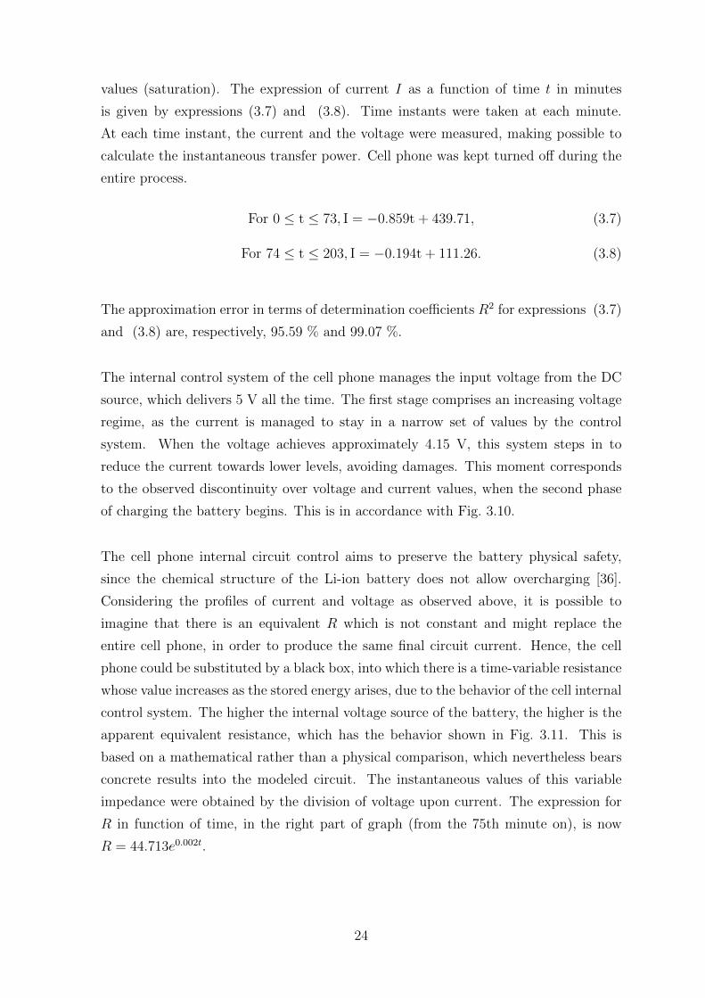
values (saturation). The expression of current I as a function of time t in minutes
is given by expressions (3.7) and (3.8). Time instants were taken at each minute.
At each time instant, the current and the voltage were measured, making possible to
calculate the instantaneous transfer power. Cell phone was kept turned off during the
entire process.
For 0 ≤ t ≤ 73, I = −0.859t + 439.71, (3.7)
For 74 ≤ t ≤ 203, I = −0.194t + 111.26. (3.8)
The approximation error in terms of determination coefficients R2 for expressions (3.7)
and (3.8) are, respectively, 95.59 % and 99.07 %.
The internal control system of the cell phone manages the input voltage from the DC
source, which delivers 5 V all the time. The first stage comprises an increasing voltage
regime, as the current is managed to stay in a narrow set of values by the control
system. When the voltage achieves approximately 4.15 V, this system steps in to
reduce the current towards lower levels, avoiding damages. This moment corresponds
to the observed discontinuity over voltage and current values, when the second phase
of charging the battery begins. This is in accordance with Fig. 3.10.
The cell phone internal circuit control aims to preserve the battery physical safety,
since the chemical structure of the Li-ion battery does not allow overcharging [36].
Considering the profiles of current and voltage as observed above, it is possible to
imagine that there is an equivalent R which is not constant and might replace the
entire cell phone, in order to produce the same final circuit current. Hence, the cell
phone could be substituted by a black box, into which there is a time-variable resistance
whose value increases as the stored energy arises, due to the behavior of the cell internal
control system. The higher the internal voltage source of the battery, the higher is the
apparent equivalent resistance, which has the behavior shown in Fig. 3.11. This is
based on a mathematical rather than a physical comparison, which nevertheless bears
concrete results into the modeled circuit. The instantaneous values of this variable
impedance were obtained by the division of voltage upon current. The expression for
R in function of time, in the right part of graph (from the 75th minute on), is now
R = 44.713e0.002t.
24
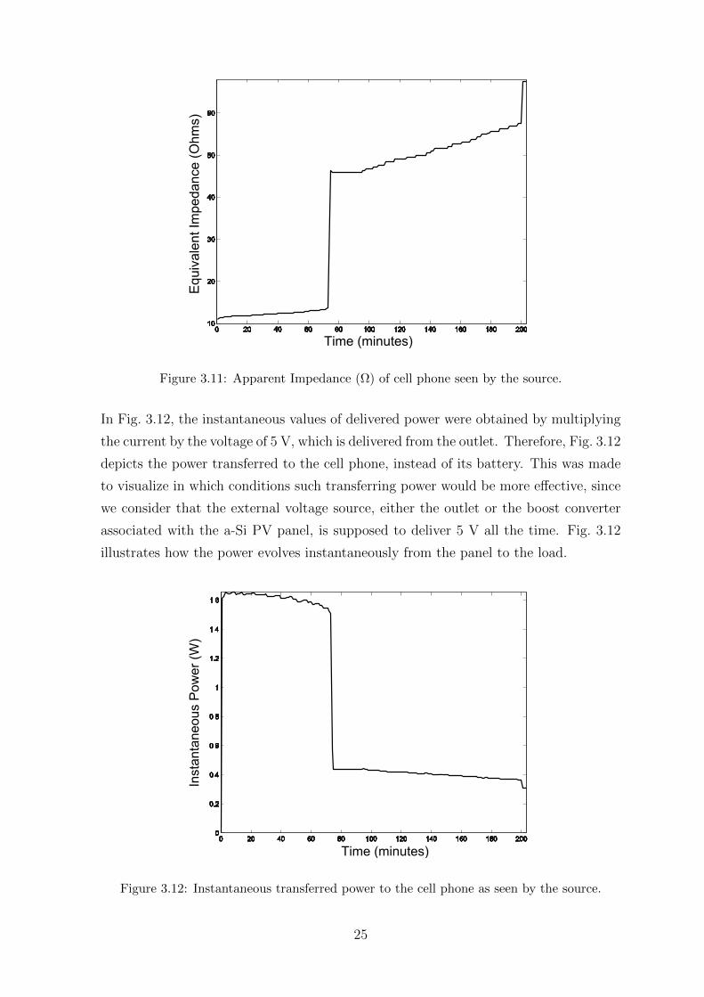
Figure 3.11: Apparent Impedance (Ω) of cell phone seen by the source.
In Fig. 3.12, the instantaneous values of delivered power were obtained by multiplying
the current by the voltage of 5 V, which is delivered from the outlet. Therefore, Fig. 3.12
depicts the power transferred to the cell phone, instead of its battery. This was made
to visualize in which conditions such transferring power would be more effective, since
we consider that the external voltage source, either the outlet or the boost converter
associated with the a-Si PV panel, is supposed to deliver 5 V all the time. Fig. 3.12
illustrates how the power evolves instantaneously from the panel to the load.
Figure 3.12: Instantaneous transferred power to the cell phone as seen by the source.
25

One may notice that the most favourable situation to transfer energy to the cell phone
occurs during the final part of the saturation stage. Since the apparent impedance
arises, the cell phone will draw a lower current, diminishing the probability of voltage
to plunge, considering that the source is a solar panel. Hence, hereafter we adopt
the premise according which the higher is the energy stored in the battery (higher
equivalent impedance), the more effective will be the power transfer. This corresponds
to the right part of the graphic shown in Fig. 3.11. Furthermore, the PV panel has a
higher internal impedance, and such characteristic offers the possibility of increasing
the impedance load and the power simultaneously.
3.2.4 Indoor Experiment Using Artificial Light and Results
In this experiment, the cell phone is charged considering indoor light. In order to
perform measurements in indoor scenarios, the environment in Figure 3.13 is suggested.
This figure shows an office-desk with a lamp in its support. The a-Si panel was installed
on the bottom of the lamp support, inside of which an 8 W LED lamp was installed to
provide artificial light. The center of the LED lamp was considered to be 13 cm apart
from one of the panel borders. The cell phone is connected to the solar panel and a
boost converter, using it as its charger, in the same way while charging it directly by
the grid.
Figure 3.13: Overall deployment of cell phone, amperimeter (in series) and solar panel undera light-support in an office for electrical current measurement.
An enlarged solar panel, which delivers 2.8 V (Vi) and power of 3.92 W at lower
luminosities, was considered. These hypothetical values for the panel aim to allow the
examination of possible results in the recycling process. Moreover, the panel concerning
to this stage of the experiment is made of two modules of 24 cm x 35 cm each (therefore,
0.168 m2 of total area). Considering the environment of Figure 3.13, light beam must
26
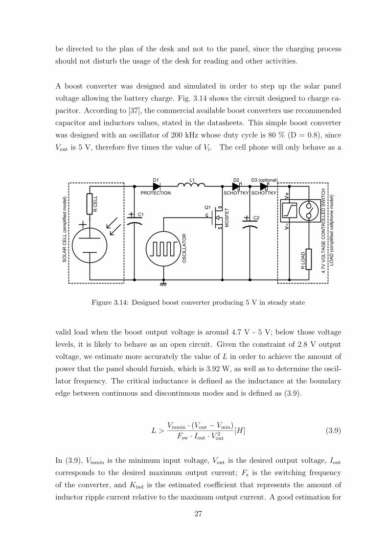
be directed to the plan of the desk and not to the panel, since the charging process
should not disturb the usage of the desk for reading and other activities.
A boost converter was designed and simulated in order to step up the solar panel
voltage allowing the battery charge. Fig. 3.14 shows the circuit designed to charge ca-
pacitor. According to [37], the commercial available boost converters use recommended
capacitor and inductors values, stated in the datasheets. This simple boost converter
was designed with an oscillator of 200 kHz whose duty cycle is 80 % (D = 0.8), since
Vout is 5 V, therefore five times the value of Vi. The cell phone will only behave as a
D1 D2 D3 (optional)
C1C2
Q1
R L
OA
D
R C
ELL
MO
SF
ET
OS
CIL
LAT
OR
LOA
D (
sim
plifi
ed c
ellp
hone
mod
el)
SO
LAR
CE
LL (
sim
plifi
ed m
odel
)
4.7V
VO
LTA
GE
CO
NT
RO
LLE
D S
WIT
CH
PROTECTION
L1
SCHOTTKY SCHOTTKY
Figure 3.14: Designed boost converter producing 5 V in steady state
valid load when the boost output voltage is around 4.7 V - 5 V; below those voltage
levels, it is likely to behave as an open circuit. Given the constraint of 2.8 V output
voltage, we estimate more accurately the value of L in order to achieve the amount of
power that the panel should furnish, which is 3.92 W, as well as to determine the oscil-
lator frequency. The critical inductance is defined as the inductance at the boundary
edge between continuous and discontinuous modes and is defined as (3.9).
L >Vinmin · (Vout − Vmin)
Fsw · Iout · V 2out
[H] (3.9)
In (3.9), Vinmin is the minimum input voltage, Vout is the desired output voltage, Iout
corresponds to the desired maximum output current; Fs is the switching frequency
of the converter, and Kind is the estimated coefficient that represents the amount of
inductor ripple current relative to the maximum output current. A good estimation for
27

the inductor ripple current is 20 % to 40 % of the output current, that is, 0.2 < Kind <
0.4. Considering feeding cell phone with power, Vout = 5 V. It was adopted Kind =
0.3, Fsw = 200 kHz and Vinmin = 1.0 V, with Iout = 100 mA. The resultant minimum
value is 26 µH. If our choice for Vinmin is 1.16 V, then the minimum L is 32 µH. These
observations allow us to choose an inductor of 33 µH.
According to [38], since the capacitor’s equivalent series resistance (ESR) affects effi-
ciency, low-ESR capacitors will be used for best performance. A load resistance of 50 Ω
was adopted, according to the verified values for R in the beginning of the second stage
of Fig. 3.11. An approximated expression for the required capacitance as a function of
ripple voltage requirement, ∆Vout, D, switching frequency Fs and output voltage, Vout
is given by
C ≥ Vout ·DFs ·∆Vout ·R
. (3.10)
Considering ∆Vout, which is the maximum ripple output voltage, as 5 % (or 0.05),
assuring the minimum output voltage to stay over 4.75 V, the minimum value of output
capacitor is 8 µF. Since the constant RC, shown in (3.11), requires commonly a higher
value for resultant C in order to avoid the deterioration of voltage value, it is possible
to choose C2 to be 20 µF.
However, with these values of R and C2, even when C1 equals 100 µF the result makes
Iout to decay less than 0.5 %. Considering that low levels of resistance load might
demand higher capacitances in order to avoid Iout to lower significantly, the value of
C1 is chosen to be 100 µF. All the components are part of the circuit shown in Fig. 3.14.
ic =E
Re−
tRC (3.11)
Fig. 3.15 depicts the blue line which represents the boost output voltage, whereas the
black line shows the effective values of voltage and current absorbed by the cell phone.
Considering the conditions of the boost and the panel, which must provide 2.8 V
minimum, the time to achieve steady state does not overcome 0.3 ms.
In a limited voltage current source, as the solar panel, in the flat part of the V x
I graphic, the bulkier the resistance coupled, the higher is the power transferred to
28
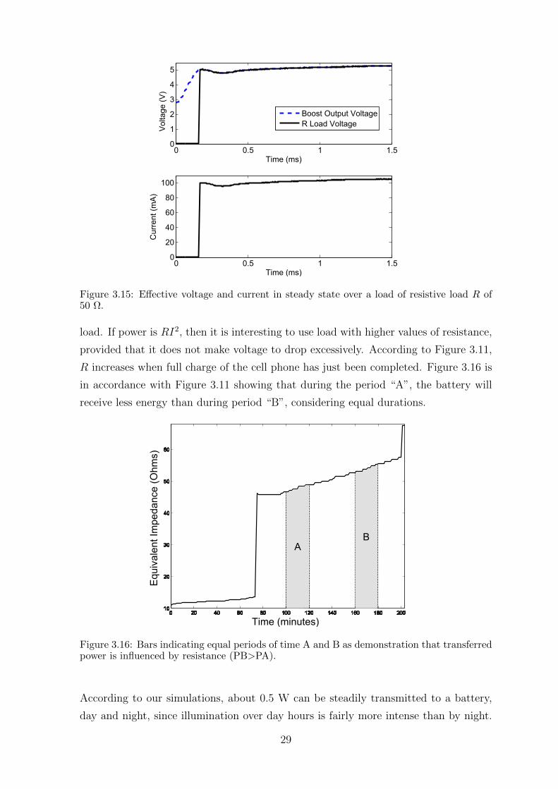
0 0.5 1 1.50
1
2
3
4
5
Time (ms)V
olta
ge (
V)
0 0.5 1 1.50
20
40
60
80
100
Time (ms)
Cur
rent
(m
A)
Boost Output VoltageR Load Voltage
Figure 3.15: Effective voltage and current in steady state over a load of resistive load R of50 Ω.
load. If power is RI2, then it is interesting to use load with higher values of resistance,
provided that it does not make voltage to drop excessively. According to Figure 3.11,
R increases when full charge of the cell phone has just been completed. Figure 3.16 is
in accordance with Figure 3.11 showing that during the period “A”, the battery will
receive less energy than during period “B”, considering equal durations.
Figure 3.16: Bars indicating equal periods of time A and B as demonstration that transferredpower is influenced by resistance (PB>PA).
According to our simulations, about 0.5 W can be steadily transmitted to a battery,
day and night, since illumination over day hours is fairly more intense than by night.
29
It can be noticed that in just one day (24 hours) the proposed system can return
12 Wh to a battery, which overcome the overall energy needed to its full charge, which
is approximately 3.72 mWh. Much more than this can be achieved by just making
smaller the distance between lamp and the a-Si panel: being the panel 1.5 cm closer
to the LED lamp, current increased 36 % and, therefore, 85 % in power.
Our simulations will consider two cases: solar panel will generate power only from
inside houses and buildings, and therefore we can consider to produce 12 Wh per day
and per square meter. Despite our panel has 0.168 m2, the enhancement of this area
will not likely result in additional energy to be drawn; 168 cm2 probably occupies a
single lamp completely. For the sake of conservatism, we will adopt 1 m2 of a-Si panel
to generate the amount of 0.5 W continuously. A second simulation is also projected: in
this situation, the panel will harvest power from indoor light only at night, generating
energy outdoor during the day hours. In order to provide the respective energetic
measurement, the next section is developed.
3.2.5 Expected results for outdoor environments
According to [39], monocrystaline, policrystaline and amorphous silicon solar cells are
capable to produce, in the Maximum Power Point (MPP), an electric current of about
32 mA/cm2, being the voltage in the range [0.46 V 0.48 V]. Cells arranged in parallel
sum the current, whereas cells arranged in series sum voltage. Taking into account
1 m2 we can put in position 64 modules of 156cm2 in series, for example, obtaining
5.0 A over [29.44 V 30.72 V], resulting in [147.2 W 153.6 W]. This values are in
accordance with the commercial specifications of module 80 Wp, which has dimensions
0.6 m × 1.0 m.
Standard Test Conditions (STC) include irradiance of 1.000 W/m2, Air Mass (AM)
1.5 and temperature of 25C. Values of MPP are calculated by the manufacturer under
STC. These considerations allow us to adopt the overall average efficicency of 15 %, i.
e., for each incident 100 W onto the PV panel, approximately 15 W will be effectively
converted into useful power.
Photovoltaic generators may provide power which vary in function of the external
conditions they undergo, the intensity of incident light and the ambient temperature.
These data are supposed to oscillate substantially in a single day and from one day to
another. Information about broader periods can help to achieve average results. Since
30

the application of this study is thought to be in a Brazilian city, we resort to [40] in
order to obtain the distribution of global daily irradiations in annual averages, which
is shown in Table 3.4.
Table 3.4: Annual Average of Daily Irradiance [Wh/m2] by Brazilian Region [40].
Brazilian Geographic Region Annual Average of Global Irradiance [Wh/m2]
North 5462
North-East 5688
Middle-West 5630
South-East 5478
South 5015
This set of values justifies the adoption of 5000 Wh/m2 as the total incident power
originated from solar beam during a day, still being a conservative value. Crossing this
parameter with the average efficiency of 15 %, we achieve the daily available power of
750 Wh/m2. The corresponding weekly amount of energy is 5.25 kWh/m2. This value
will be taken on as the main reference related to projections for PV generation within
Brazilian cities.
3.3 Electric Eel
3.3.1 Theory
The third analyzed element, which is an energy source itself rather than a recycling
scheme, is the electric eel. This freshwater fish is rife in Amazonia and converts chemical
energy existing in their food into voltage along their body constantly, emitting higher
values when exposed to stronger stimuli. Values of voltage along the body of this
animal are creditable of investigation: a single discharge can reach several hundreds
of volts. The utilization of electric eels for energetic objectives is, nonetheless, still
inexpressive. We discuss why and feature eels’ properties in order to conceive a worthy
scenario for its employment as a renewable source.
31

3.3.2 State of the Art
3.3.2.1 Electric eel properties
Electric eels can live in freshwater. Desirable values for pH are within 5.0 - 7.0, and
water electric condutivity may vary between 30 - 100 µS, being about 25 C the ex-
pected temperature of water for the fishes lying in Amazonia [41]. Electric eels have
no lungs, but rather a respiratory organ inside the mouth. Hence, they are mandatory
air-breathers. The interval between two breathes is about five minutes. Their body
can reach 2.5m and they can weigh up to 20 kg. If they are kept in an aquarium, about
30 % of the water must be renewed in order to preserve their healthy. For electric eels,
the ideal aquarium may have 1.5m of water depth [42].
The electric eels has the scientific denomination Electrophorus electricus and bears
three electric inner organs which only act simultaneously under an attack or when the
eels aims to kill a prey, which are the cases of the strong discharge. The amplitude
of this discharge current can reach 1 ampere, for a large eel. The respective voltage
can achieve the intensity of 600 volts. Therefore, during this time, the electric eels
can emit a power of approximately 0.6 kW. However, under normal conditions, the
eel emits few volts only for seeing what exists in the environment during navigation,
and also for communicating. The chemical principle behind the voltage generation
is shown in Fig. 3.17. Inside the eel (Electrophorus) there is a modified muscle, the
electric organ, whose fundamental cellular unit is the electrocyte. These cells are very
similar to muscle fiber cells in which they can produce electric signals, but, unlike
muscle fiber cells, they cannot contract. Such cells contain a high concentration of
Potassium ions (K+), a low concentration of Sodium ions (Na+), and a comparable
amount of negatively charged ions. The cell membrane is permeable to K+ ions but
not to Na+ ions. When in this inactive state, the cell membrane has a negative voltage,
avoiding potassium ions to flow out the cell [43].
Acetylcholine, a neurotransmitter, can activate the electrocyte cells. It is secreted
through nerves on one side of the cell, causing ion channels to open on that side. Na+
ions are then able to rapidly enter the cell via these channels. This influx of positive
charge modifies the equilibrium potential of the cell. To reestablish this equilibrium,
the K+ ions leave the cell on the other side, still very permeable to K+.
About 6000 of these electrocytes cover approximately 4/5 of the eel’s body length, and
when these cells are activated, the eel produces the voltage amplitude. The head of
32

Figure 3.17: Electrocytes behavior which yields an external electric voltage: (a) cell mem-brane is permeable only to K+ ions; (b) Acetylcholine activates the electrocyte cell, makingNa+ ions to come inside it [43]. In the case of Electrophorus electricus, there exists only theposterior membrane, which is excitable.
the eel has a positive charge, and the negative charge stands on the tail. The emitting
voltage are also responsible for giving to the eels a substitutive sense of vision, as the
sonar, for a bat, since eels do not see sufficiently with the eyes. Objects having different
conductivities distort the electric field that the eel produces, thus making the eel aware
of such objects’ presence. Furtheromore, voltage discharges perform an important role
in social communication. Even the gender identification among electric eels depends on
the characteristics of discharges profile from each one of them [44]. Fig. 3.18 illustrates
the path current lines that the eels emit.
Electric eels use low values of electric current to perceive the world around them, and
they make it 24 hours daily. With regards to Fig. 3.18, any scheme of harvesting energy
from these fishes should provide conductors in proximity to the head and the tail, in
order to shorten the path of energy through water.
3.3.2.2 Available Papers
Consulting the available papers in IEEE about eels, only one paper was found [45] which
studies these fishes with regards to their capability of producing electricity. This article
provides some interestig data, as for instance the energy produced per unity of tissue
volume. Electric energy produced per cubic centimeter of tissue is 370 microjoules per
impulse in a 60-centimeter eel and only 100 microjoules per impulse in a 180-centimeter
33

Figure 3.18: Lines of electric field generated along the eel’s body. The head is the positivepole, and the tail bears the negative pole, from where electric current goes off through wateruntil the head [44].
eel. Therefore, the capability of producing energy per volume of tissue decreases with
higher volumes. Such impulses, however, are not the source of power to be considered
in this study, since we will handle the continuously emitted electrical power, whose
magnitude are in the order of few miliwatts [45].
One of the greater merits of this article is the establishment of an equivalent circuit for
the eel, which is shown in Fig. 3.19. In this model, E is the effective electromotive force
of the 10-centimeter segment of electric tissue, and r is the effective internal resistance.
R′ is the effective resistance of all closed circuits within the nonelectric tissue of the
fish, and R is the external load. The tissue is a complex network of electromotive
force and resistance. The substitution of the simple model is justified by Thevenin’s
theorem. The application implicitly assumes that E, r, R′ and R are independent of
the current.
Figure 3.19: Equivalent circuit of the electric eel [45].
34

On the best knowledge of the author, there are not experiments aiming to harvest
energy from eels with a clear market insertion model, as proposed in this study. A pos-
sible explication is that these fishes are not indicated for household captivity. Moreover,
their expected amount of energy, in steady state, seems to be not worth it in face of
the necessary investments.
3.3.3 Measurements
With the goal of harvesting energy from the eel and measuring the electric power, an
experiment was carried out in Laboratorio de Fisiologia Comportamental e Evolucao
do Instituto Nacional de Pesquisas da Amazonia (LFCE-INPA), in the city of Manaus-
AM (Brazil). An electric eel measuring about 90 cm was inserted into an aquarium
of approximated sizes 120 cm x 50 cm x 50 cm. Two plaque-shaped electrodes were
installed on each side of the larger width of the aquarium. The correspondent resistance
of each electrode is 4 Ω. Figures 3.20, 3.21 and 3.22 show, respectively, the photo from
the real experiment, a picture which describes the whole deployment of the experiment,
and the respective equivalent circuit.
Figure 3.20: Real experiment carried out in LFCE-INPA, wherein the electrodes are metalplaques with a resistance of 4 Ω each. This photo was made while the electric eel swam inorder to look for the prey, which is the little fish in the above part of the aquarium, near tothe surface.
35
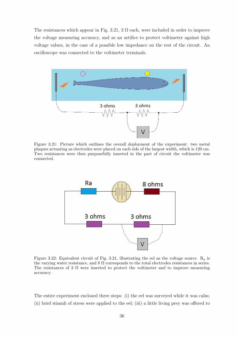
The resistances which appear in Fig. 3.21, 3 Ω each, were included in order to improve
the voltage measuring accuracy, and as an artifice to protect voltimeter against high
voltage values, in the case of a possible low impedance on the rest of the circuit. An
oscilloscope was connected to the voltimeter terminals.
Figure 3.21: Picture which outlines the overall deployment of the experiment: two metalplaques actuating as electrodes were placed on each side of the largest width, which is 120 cm.Two resistances were then purposefully inserted in the part of circuit the voltimeter wasconnected.
Figure 3.22: Equivalent circuit of Fig. 3.21, illustrating the eel as the voltage source. Ra isthe varying water resistance, and 8 Ω corresponds to the total electrodes resistances in series.The resistances of 3 Ω were inserted to protect the voltimeter and to improve measuringaccuracy.
The entire experiment enclosed three steps: (i) the eel was surveyed while it was calm;
(ii) brief stimuli of stress were applied to the eel; (iii) a little living prey was offered to
36

the electric eel. The duration of the steps (i) and (iii) was 120 seconds each, whereas
the situation (ii) lasted 60 seconds.
The values of voltage appearing in the graphs of the following subsections were obtained
by considering that the condutivity of freshwater is between 10 µS/cm and 70 µS/cm,
as stated in [46]. Electrical condutivity between 20 µS/cm and 70 µS/cm are expected.
The average value of 40 µS/cm was therefore combined with the mean distance of
the eel to the electrodes in order to characterize conveniently the resistance Ra.
3.3.3.1 Electric eel under still water
In the first situation, the electric eel was let in the aquarium with no external intentional
stimulum. This step aimed to feature the voltage along the eel’s body while it is only
recognizing the environment or trying to communicate. The eel was able to move easily
trough the aquarium. When, in a given moment, the eel turned around and swam in
the opposite direction, the recorded voltage values changed from negative values to
positive ones.
Figure 3.23: Voltage values with the eel swimming freely into the aquarium.
Voltages emitted by the eel appear in Fig. 3.23. The inversion of voltage signal is due
to the eel to turn around into the aquarium, while it swam. Electric equivalent DC
current in this situation were around 1 mA. The mean value of voltage in this stage of
37

the experiment stood around 10 V. An eel whose size is 90 cm can, therefore, in steady
state, furnish 10 mW for the power managing circuit. The advantage of the eel over
the other renewable sources is exactly the level of voltage by which power is provided,
since the other sources provide power with few milivolts.
The amount of power delivered in this situation can be enhanced by means of employing
a larger eel, since the amount of deliverable power increases with the weight of the eel,
although not linearly, as we beheld in [45]. Hence, it is valid to affirm that 10 mW in
steady state are available if no expressive losses in the aquatic path current occur.
3.3.3.2 Electric eel under stress
In this step, the eel underwent some stress. The stimuli consisted in agitating water
randomly during 60 seconds with a bar.
It is obvious that such type of stimulum is not sustainable in the long-term, since it
draws from the electric eel an amount of power that this fish cannot provide in steady-
state. As shown in Fig. 3.17, there is a physical limit for the Acetylcholine to activate
the electrocyte cell, as the amount of ions is not infinite.
Furthermore, it is not imaginable to stress the electric eel permanently, which would
be inhuman and, besides, inefficient, given that the eel could learn the external inputs
and stopping of answering as we desire it to do. The main point is that our managing
circuit must be prepared to avail the energy coming from the fish even in the stress
situation.
3.3.3.3 Electric eel receiving a prey
During this step of the experiment, a little fish was offered as a prey to the electric
eel. In the very beginning of this process, the eel emitted a large voltage pulse. In the
sequence, the electric eel decreased voltages intensity until the end of recording values.
Nevertheless the eel provided high values while it desires to kill the next meal, it
depends also on how hungry it is. Forecasting confidently the amount of energy in this
situation would be almost impossible.
38

Fig. 3.24 shows voltages values during the second and the third described situations:
(a) electric eel under stress, and (b) eel receiving a prey. One can notice that results
for voltage values in (a) are more spaced each other; on the other hand, they are more
intense.
Figure 3.24: Voltage values with (a) the eel being stressed, and (b) eel trying to kill a littleprey that is placed in the aquarium.
We consider hereafter only the values extracted from the step 1 observed in the previous
experiment. We suppose that, since electric eels can provide such values of voltage on
steady-state, they cannot furnish high values of voltage all the time. It is assumed that
the overall energy available we can reliably count on in the end of process is higher as
the variance of voltage values is lower.
3.3.3.4 Structure for electric eels energy harvesting
The premise according which at least 30 % of the water must be renovated weekly rises
questions of the energetic cost in doing so. The ideal situation is not expending energy
with this activity. Captivity systems are likely to demand this water to be changed
and, therefore, imposing an undesirable energetic duty.
This study considers to keep electric eels in the river, generating energy from there. As
shown in experiment under still water, eels emit a “stand-by” voltage 24 hours daily,
indicating therefore the amount of electrical power we can steady count on. Despite
39

in this case the electric eels produce voltage values that are considerably lower, such
energy is considered reliable.
One solution is to build a structure within which the eels could swim with no hin-
drances, but not being allowed to execute large displacements. The system illustrated
in Fig. 3.25 comes up as a possible solution. It consists on a basket with no obstacles to
the water to flow inside it, working as a swimming-pool since it constrains the electric
eels to go out. So, water can come in and out of this structure, unlike the eels. It is
supposed to work as a type of corral for the electric eels inside it. The surface of water
should stand approximatley on the half height of it, enabling the eels to come upwards
to breathe. Two conductive structures must be installed into this aquarium-corral:
one of them consists in a nude wire circumscribing the inner part of the walls. The
other metal piece is again a nude wire which circumscribes a cylinder installed in the
middle of the struture, so that it remains fixed in the center of the swimming area.
Both cable in the inner part of the walls and cable fixed on the central cylinder have
to be connected to external terminals of a battery, so that one must reach the positive
pole and the other must connect the negative pole of the battery. Alternatively, the
cables in this basket can be substituted by conductive bars.
Figure 3.25: Perspective view of the basket, or aquarium-corral. The brown lines representconductors, either nude cable or bars, each one being connected to a different polarity of theexternal circuit of power management.
Fig. 3.25 depicts the perspective of the basket. Fig. 3.26 illustrates the upper view,
without (a) and with the eel (b). One can notice that, no matter the point of the
aquarium-corral the eel is, both the head and the tail are near, respectively, to one
40

Figure 3.26: Upper views of the basket: (a) view of the basket without eels inside; (b) viewof the basket with one eel swimming inside the corral. At any moment of the displacementof the eel, both head and tail are likely to be near to the collecting current points, which arethe conductive cables.
wall and to the central cylinder. This proximity is of great interest given that it seeks
to mitigate the impact of Ra, which is the resistance of the water path current.
In what concerns to the eels in this dissertation, we shall assume the overall harvesting
scheme which is represented in Fig. 3.27. A bundle of baskets are deployed along a
river which crosses the city, each basket containing one or more electric eels inside it.
Connecting cables, either in parallel or in series, gather the energy coming from the
baskets, leading them to the nearest Power Substation. The PS then manages the total
eels instantaneous power and then injects it in the grid.
3.3.3.5 Eels available power
Electric eels under still water provide 10 mW steadily, as illustrated in Fig. 3.23 if we
consider the average current of 1 mA.
The number of electric eels to be distributed along the river can vary reasonably.
Despite the indeterminate number, a set of assumptions are welcome at this point.
One assumption refers to the number of eels by basket: two or more eels can draw
the electrical current among them, so that it is perhaps worth avoid joining eels in the
same corral. As such, one electric eel per basket is assumed as a premise.
Other aspect is related to the form by which the energy produced by the eels will be
stored. This dissertation aims to predict the series of maximum power demand values,
41

Figure 3.27: Proposed scheme for energy harvesting from eels in a river, which comprises eelsinside the baskets. All the output cables are connected to a power manager circuit, whichcarries out this power to be conditioned.
which are likely to occur during the peak, i. e., the hours of the day in the end of
afternoon and beginning of evening. In Brazil, the peak starts at 17h30, in average,
and always lasts for 3 hours. If the eels produce energy along all the day and the
power is used immediately, with no batteries in the substation to gather it up, then
the amount of power received from the eels will vary around Pe = 0.01ne [W], where
Pe is the power furnished by the eels and ne is the number of eels.
Diversely, if the power can be stored, we can concentrate the Watts produced during 23
hours of the day and inject it into the grid only during one of the 3 peak hours. We can
assume that for each 24 hours of storing energy, in only one hour we will use the energy.
As such, say that the Pe−peak = 24ne [W], where Pe−peak is the power delivered by the
batteries solely during the peak. Moreover, the period of one hour here described does
not need to be continuous: it can be sliced over 15, 10 or 5 minutes, preferentially
when the higher values of power demand are observed.
The importance of this consideration for our purposes is related to optimizing eels
energy. Maximum power demand values are highly likely to occur during the peak. If
we imagine we have 400 electric eels connected to one PS, storing energy all the day
results in Pe−peak = 400 × 24 × 0.01 = 98 W. This amount of power is near to 0.15 %,
42

in many cases, of the most severe peak values.
Undoubtedly, there must be a coefficient of storage losses, but it will be taken for
slight due to the main goal of this study, which is about time series prediction, and
because the size of our electric eel, being 90 cm long, may suffer changes. Therefore,
as another result of this chapter, the energy will be considered to be Pe−peak = 24ne
[W], as above-mentioned.
3.4 Summary of the three energetic sources
Table 3.5 provides a little scheme with a global view upon the main energetic charc-
teristics of each source. The RF energy harvester system, indoor light recycling circuit
and electric eels have different profiles, according to the Table 3.5. All those are weekly
results.
Table 3.5: Summary about three energetic sources: RF harvesters, indoor light recycling,electric eels.
Source RF antennas Indoor light Solar PV Eels
Daily hours of power (h) 24 12 12 24
Generation(G)/Recycling(R) R R G G
Weekly produced energy 0.144 Wh/ant. ∗42 Wh/m2 5250 Wh/m2 1.68 Wh/eel
∗ 42 Wh/m2 refers to the weekly energy from indoor light when the panel is used only
12 hours a day. In the case we harvest indoor energy 24 hours, the result is 84 Wh/m2.
43

Chapter 4 ENERGY DEMAND PREDICTION IN A
STANDARD ELECTRIC POWER GRID
4.1 Overview
As said in Chapter 1, two stages of measuring are undertaken along this dissertion. The
first stage handles power demand prediction with no renewable microgeneration sources
being considered. Microgeneration sources are included only in the model during the
second stage, which is described and developed in Chapter 5.
This chapter runs upon the first stage, in which Auto-Regressive (AR) model, Auto-
Regressive with eXogeneous Inputs (ARX), Auto-Regressive Moving Average with eXo-
geneous Inputs (ARMAX) and Artificial Neural Networks (ANN) system are compared
to each other, in order to determine which one is more suitable for predict data.
In what concerns to physical maintenance of the grid assets and energy quality, the
most important parameter is the maximum power registered, since it indicates the
most severe situation that the grid must to attend satisfactorily. Mean power data
are more likely to be useful for economic analyses and about the evolution of market
consumption. In this study, we consider that the maximum values prediction is the
core activity, and therefore all the efforts will be dedicated to forecast its values. Thus,
from now on, if we say “value” or “demand value” as isolated expressions, they must
be understood as the maximum power demand in the respective week.
Eight PSs in Leipzig, Germany, had their demands registered from 2001 to 2004. These
4 years yield 209 registers for each PS. All power demand values were originally recorded
in periods of 15 minutes each, emboding therefore sets of 96 daily power registers. From
this domain, each upper daily value was fetched, and the maximum weekly power
demand was the higher value among the seven daily maxima between sunday and
saturday. Therefore, we hereafter consider only these maximum weekly values, which
come from realistic meaurements from Leipzig city, in order to proceed to weekly
demands prediction. The matrix corresponding to the demand values is therefore 209
× 8, since there are 209 weeks for the 8 PSs. The experiment with Box & Jenkins
models and ANN systems predict values only for the last 9 weeks for each Substation.
44
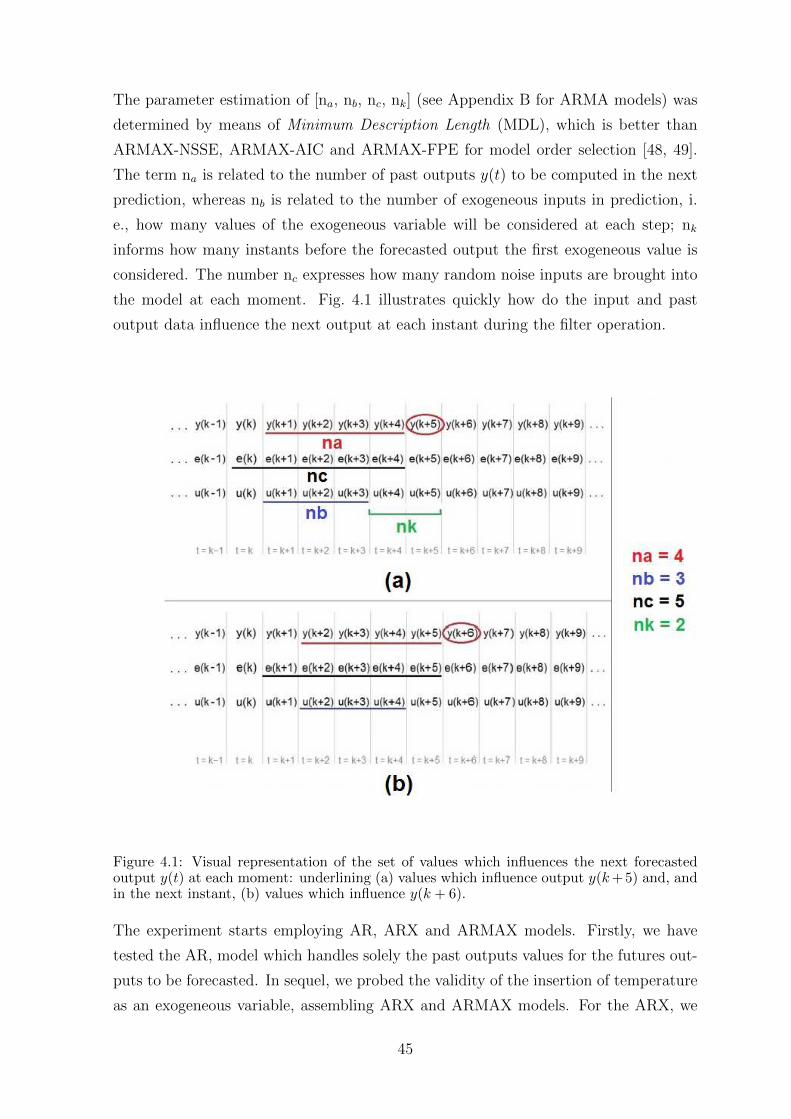
The parameter estimation of [na, nb, nc, nk] (see Appendix B for ARMA models) was
determined by means of Minimum Description Length (MDL), which is better than
ARMAX-NSSE, ARMAX-AIC and ARMAX-FPE for model order selection [48, 49].
The term na is related to the number of past outputs y(t) to be computed in the next
prediction, whereas nb is related to the number of exogeneous inputs in prediction, i.
e., how many values of the exogeneous variable will be considered at each step; nk
informs how many instants before the forecasted output the first exogeneous value is
considered. The number nc expresses how many random noise inputs are brought into
the model at each moment. Fig. 4.1 illustrates quickly how do the input and past
output data influence the next output at each instant during the filter operation.
Figure 4.1: Visual representation of the set of values which influences the next forecastedoutput y(t) at each moment: underlining (a) values which influence output y(k+ 5) and, andin the next instant, (b) values which influence y(k + 6).
The experiment starts employing AR, ARX and ARMAX models. Firstly, we have
tested the AR, model which handles solely the past outputs values for the futures out-
puts to be forecasted. In sequel, we probed the validity of the insertion of temperature
as an exogeneous variable, assembling ARX and ARMAX models. For the ARX, we
45

tested temperature and logarithm of temperature values. This step was helpful since
the prior supposition is that electric consumption increases with lower temperatures,
in cold weather countries, as Germany. Fechner’s law states that subjective sensation
is proportional to the logarithm of the stimulus intensity [50]; therefore, since human
perception of cold is logarithmic [51], we tested the suitability of the logarithm of
temperature as a better exogeneous variable.
After determining na and nb by means of MDL, we have established the number of
entries for the ANN system. The reason for determining na and nb at prior is due to
the intended perfect paralell comparison between ARMAX and ANN: if we want to
predict values based on the na and nb terms, it is worth to fix the same input data
for ANN. Clearly, we are considering that the same input values are likely to produce
output values also in the ANN system.
The ANN structure is a Multi-Layer Perceptron (MLP) mesh of two hidden layers. Our
MATLAB codes ran in order to achieve the best number of neurons in each hidden layer,
limiting them to 6 neurons maximum. The ANN forecasts were based on these optimal
quantity of neurons per layer. Then, the resulting MLP underwent the trainning period
(first 200 weeks), returning outputs for the last 9 weeks. As far as we can see, our ANN
system provided the best results for an ANN system bearing two layers, with 200 input
data for the following 9 data forecasting.
The indicative numbers of each one of the 8 PSs are hereafter described by letters from
A to H, by means of the following correspondence: A = 1104, B = 1108, C = 1109, D
= 3092, E = 3219, F = 3244, G = 4012, H = 4254.
Consumption Data by Power Substation (PS). The 8 observed PSs present
weekly maximum power demands as shown in Figure 4.2. The first week contains
January 1st 2001 and the 209th week contains December 31st 2004. The length of
demands vary over time, but the pattern is quite repetitive: as time indication ap-
proaches multiples of 52, there being the end of year and the coldest weeks of winter,
electric consumption is enhanced. This fact inspired us to seek the participation of
temperature as a relevant exogeneous input variable. In Fig. 4.2, graph for Substation
H illustrates the period of time the forecast upon which forecasts will be done, for both
AR models and ANN system, and for each one of the 8 PSs.
46

Figure 4.2: Maximum electric power demands over the 209 weeks: letters on the top indicatethe PS. Yellow bar on H substation graph shows the forecasted period for every PS.
47

4.1.1 AR, ARX and ARMAX Models
First of all, we are supposed to seek the orders na for AR model, and na, nb and nk
for ARX and ARMAX. One can find na and nb given the delay factor nk; however,
nk is still undefined. One might adopt nk = 1, in order to forecast the next week
power demand; alternatively, nk = 9 makes sense if we are going to forecast the 9 last
weeks of the entire period. As a counterpoint, very large values of nk are likely to
limit our forecasting power, since it shortens the amount of available input data. The
exogeneous information which is going to be considered in this study is temperature in
its real and logarithmic values.
Encoutering nk was possible by means of computing loss functions for ARX models of
different orders. A loss function LF is calculated for each combination [na nb nk]. For
each hypothetical nk, we have assembled a matrix V , which is a matrix (na × nb +
1) × (4), whose lines are possible sets of [na nb nk LF ]. Then, for each different nk, a
combination na nb was assigned taking into account the minor value of LF.
In sequel, we varied nk from 1 until 208, given that we have taken on 209 sequenced
values. We have thus obtained 208 LFs. We picked the smallest overall LF in order to
achieve the final set [na nb nk].
For every PS, one different V matrix was assembled, and therefore we should obtain a
different set of [na nb nk] for each different PS. However, all values coincided: na = 10,
nb = 10 and nk = 1, being the optimal model for the 8 surveyed PSs.
Let us look at one of ARMAX generated equations to notice the role of each element,
including nc, the moving average factor. For Power Substation G, the following set of
expressions was achieved.
A(z) = 1 - 0.5861 z−1 − 0.6502z−2 − 0.5762z−3 − 0.3488z−4 + 0.8517z−5 + 0.6843z−6 +
0.2958z−7 − 0.04026z−8 − 0.8855z−9 + 0.2598z−10,
B(z) = -229.8 z−1 + 118.4z−2 − 27.16z−3 + 407.6z−4 + 17.88z−5 − 250.2z−6 −100.3z−7 − 7.266z−8 − 90.54z−9 + 161.4z−10,
C(z) = 1 - 0.2894 z−1 − 0.5455z−2 − 0.9145z−3 − 0.7849z−4 + 0.6069z−5 + 0.8731z−6 +
0.5833z−7 + 0.4015z−8 − 0.9066z−9 − 0.0225z−10.(4.1)
48
The meaning of [na nb nc nk] becomes clearer now: there are na = 10 elements in
A(z), the auto-regressive component. Other nb = 10 elements come from the exoge-
neous input variable, which is delayed in nk = 1 instant. The first element of B(z),
[−229.8z−1], is delayed in one instant in relation to the first element of A(z), which is
1. For the set of expressions in (4.1), Akaike FPE is 370.8 and fit to estimation data
is 57.14%. Fit estimation data corresponds to the prediction focus.
If we made nc = 1, instead of nc = 10, Akaike FPE would be 518.7, and the prediction
focus would fall to 49.72%. On the other hand, making nk=9, with na = nb = nc = 10,
we would produce FPE = 448.2 and a prediction focus of -331.9%. These observations
proves the reasonableness of our choice in equalizing na = nc. One interesting aspect
in selecting nk = 1 is that it allows to enlarge our set of input data, since large values
for nk constrains our first possible exogeneous input to come in the system only in the
occurence y(b+ k + 1), given that the exogeneous input set of values is complete only
in this moment.
4.1.1.1 eXogeneous Input: Temperature
After determining the general model order, we compare now AR with two ARX models,
being the first ARX dependent on temperature data and the second ARX dependent on
logarithm of temperature 1. The logarithm was obtained by means of summing 273 C
to the pure temperature data and, in sequel, applying the logarithm upon the result,
in order to avoid problems with Celsius negative values. We probed if temperature
has a logarithmic impact, in face of human perception. After that, an ARMAX model
was tested with the same parameters na, nb and nk; the parameter nc, related to the
Moving Average component, received the same value for na, which corresponds to the
number of past input values.
We have examined performances of AR, ARX (X = Temperature) and ARX (X = Log
Temperature) with two goals: testing if the addition of an exogeneous input would
really be advantageous, and, whether positive, assessing if the Log Temperature would
actually overcome Temperature as a good exogeneous variable.
Table 4.1 shows the set of results to each one of the 8 Power Substations. Prediction
focus is higher the more accurate is the model, and assumes greater values for ARX with
1Temperature data were obtained from http://www.wunderground.com/
49
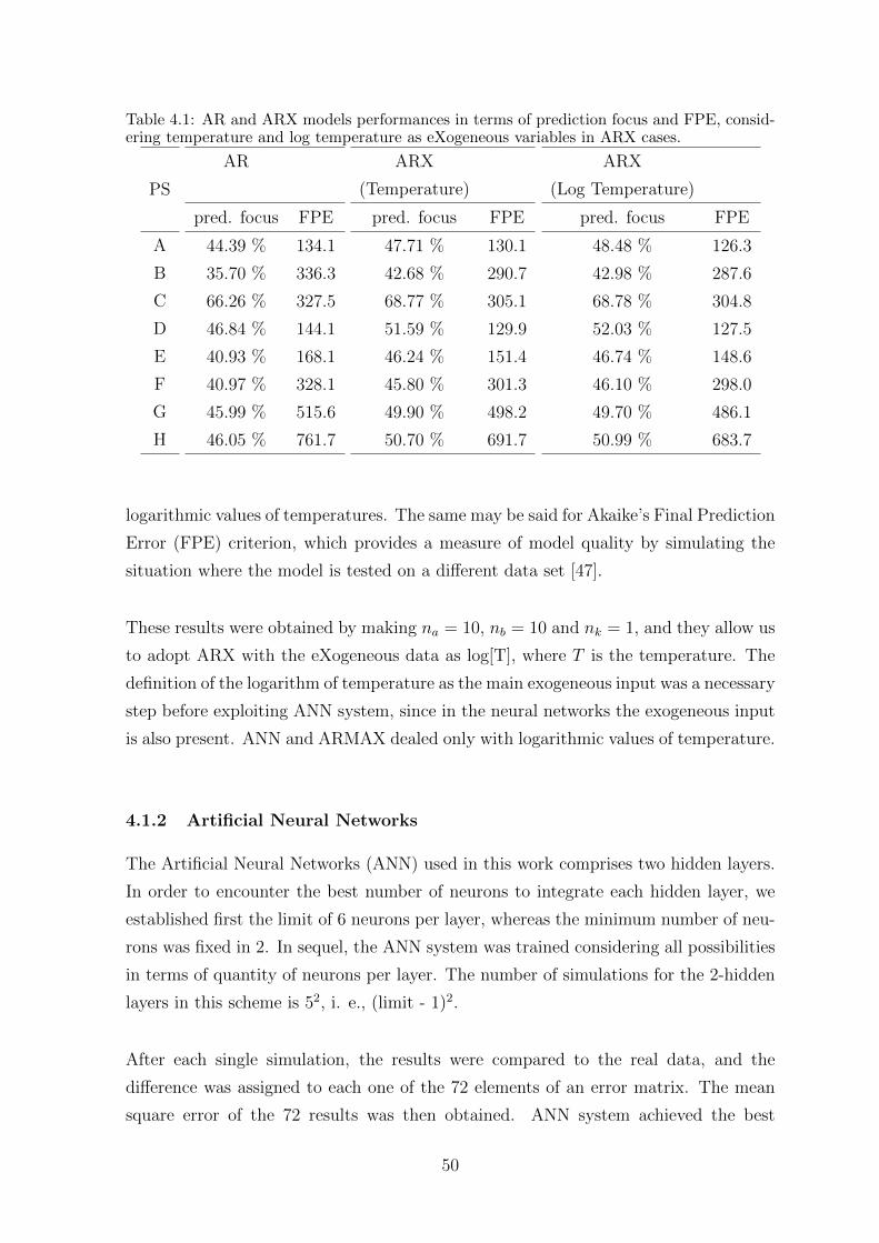
Table 4.1: AR and ARX models performances in terms of prediction focus and FPE, consid-ering temperature and log temperature as eXogeneous variables in ARX cases.
PS
A
B
C
D
E
F
G
H
AR
pred. focus FPE
44.39 % 134.1
35.70 % 336.3
66.26 % 327.5
46.84 % 144.1
40.93 % 168.1
40.97 % 328.1
45.99 % 515.6
46.05 % 761.7
ARX
(Temperature)
pred. focus FPE
47.71 % 130.1
42.68 % 290.7
68.77 % 305.1
51.59 % 129.9
46.24 % 151.4
45.80 % 301.3
49.90 % 498.2
50.70 % 691.7
ARX
(Log Temperature)
pred. focus FPE
48.48 % 126.3
42.98 % 287.6
68.78 % 304.8
52.03 % 127.5
46.74 % 148.6
46.10 % 298.0
49.70 % 486.1
50.99 % 683.7
logarithmic values of temperatures. The same may be said for Akaike’s Final Prediction
Error (FPE) criterion, which provides a measure of model quality by simulating the
situation where the model is tested on a different data set [47].
These results were obtained by making na = 10, nb = 10 and nk = 1, and they allow us
to adopt ARX with the eXogeneous data as log[T], where T is the temperature. The
definition of the logarithm of temperature as the main exogeneous input was a necessary
step before exploiting ANN system, since in the neural networks the exogeneous input
is also present. ANN and ARMAX dealed only with logarithmic values of temperature.
4.1.2 Artificial Neural Networks
The Artificial Neural Networks (ANN) used in this work comprises two hidden layers.
In order to encounter the best number of neurons to integrate each hidden layer, we
established first the limit of 6 neurons per layer, whereas the minimum number of neu-
rons was fixed in 2. In sequel, the ANN system was trained considering all possibilities
in terms of quantity of neurons per layer. The number of simulations for the 2-hidden
layers in this scheme is 52, i. e., (limit - 1)2.
After each single simulation, the results were compared to the real data, and the
difference was assigned to each one of the 72 elements of an error matrix. The mean
square error of the 72 results was then obtained. ANN system achieved the best
50

performance for 6 neurons in the first layer and 2 neurons within the second hidden
layer. Such deployment of neurons was adopted as that one which would give us the
final best result coming from our ANN system.
Input data for our ANN system were similar to the input data for AR models as
possible. Since the obtained AR schemes receive data from 10 past outputs and 10
exogeneous values, the same was made with respect to the ANN system. Therefore,
for each trainning/validation step, given an expected result y(t), we counted on 10 past
output values, y(t − 1) until y(t − 10), and 10 past exogeneous input values, u(t − 1)
until u(t − 10), in the same way it was carried out for ARX models. No noise was
added, hence nc = 0.
4.1.3 Comparison Between AR, ARX, ARMAX and ANN Results
After predictions, we achieved the error for each element of the forecasted 9 × 8 matrix.
This error matrix consists in the forecasted values by AR, ARX, ARMAX and ANN,
subtracted by the realistic power demands. One error matrix was assembled for each
model.
In sequel, we calculated the Mean Square Error (MSE), that is, the sum of all squared
errors divided by 72, the number of matrix elements. Another criterion was also tested:
the number of forecasted results standing above the real power demand value, yielding
a “Positive Deviation”. This value constitutes an important outcome, since our aim is
to prevent maximum power values in the grid. This criterion is therefore called security
criterion. The Number of Positive Deviations (NPD) is the amount of predictions which
stood above the effective maximum weekly demand.
For na = nb = nc = 10 and nk = 1, ARMAX model presented the best performance
among all tested models. Table 4.2 shows MSE and NPD values for AR, ARX, ARX
log[T] and ARMAX log[T], where log[T] indicates that the model considers the loga-
rithm of temperature as the exogeneous variable.
One may notice that the MSE increases from ARMAX to ARX log[T], continuing to
raise through ARX, AR and ANN. The number of values above the real measured
ones, NPD, follows the same sequence. One observation we must do is that the ideal
NPD would be 36, in face of the mathematical accuracy; the further from 36, the more
biased is the method, because it means that our final outputs stay sistematically below
51

Table 4.2: Mean Square Errors (MSE) and Number of Positive Deviations (NPD) for AR,ARX, ARX log[T] and ARMAX log[T], na = 10, nb = 10 and nk = 1
Parametro AR ARX ARX log[T] ARMAX log[T] ANN
MSE 2.7409 2.6457 2.5800 2.1771 4.6844
NPD 29 29 32 38 21
or above the target. ARMAX is the less biased, whereas ANN seems to be the most
one. Since our specific goal is to provide the grid to support occasional extra power
demands with optimal investments, we can elect NPD parameter as important for our
purposes.
Absolute values of prediction deviations with regards to the real values were also re-
gistered in order to provide an effective comparison among all models. Matching all
models to each other, we assigned a combination of PS/week whose result is the name
of the model which provided the lowest absolute value for the error. The overall result
is shown in Figure 4.3. The superiority of ARMAX is patent: ARMAX prevailed
in 34 occurrences, or 47.22 % of the 72 events. The model which has provided the
second more accurate set of results was AR, with 12 occurrences (16.67 %). Both ARX
log[T] and ANN appeared 9 times (12.50 % each), whereas ARX has shown up 8 times
(11.11 %).
Figure 4.3: Models which have provided the minor deviation absolute values, for each weekand PS.
52
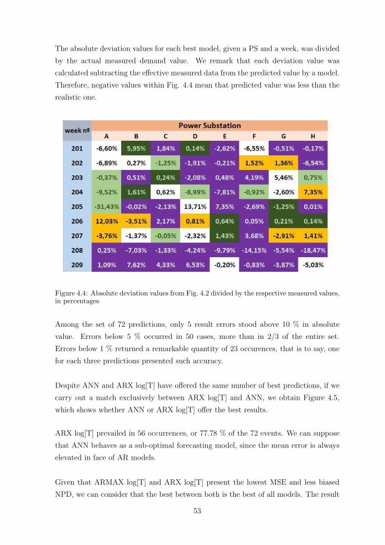
The absolute deviation values for each best model, given a PS and a week, was divided
by the actual measured demand value. We remark that each deviation value was
calculated subtracting the effective measured data from the predicted value by a model.
Therefore, negative values within Fig. 4.4 mean that predicted value was less than the
realistic one.
Figure 4.4: Absolute deviation values from Fig. 4.2 divided by the respective measured values,in percentages
Among the set of 72 predictions, only 5 result errors stood above 10 % in absolute
value. Errors below 5 % occurred in 50 cases, more than in 2/3 of the entire set.
Errors below 1 % returned a remarkable quantity of 23 occurences, that is to say, one
for each three predictions presented such accuracy.
Despite ANN and ARX log[T] have offered the same number of best predictions, if we
carry out a match exclusively between ARX log[T] and ANN, we obtain Figure 4.5,
which shows whether ANN or ARX log[T] offer the best results.
ARX log[T] prevailed in 56 occurrences, or 77.78 % of the 72 events. We can suppose
that ANN behaves as a sub-optimal forecasting model, since the mean error is always
elevated in face of AR models.
Given that ARMAX log[T] and ARX log[T] present the lowest MSE and less biased
NPD, we can consider that the best between both is the best of all models. The result
53
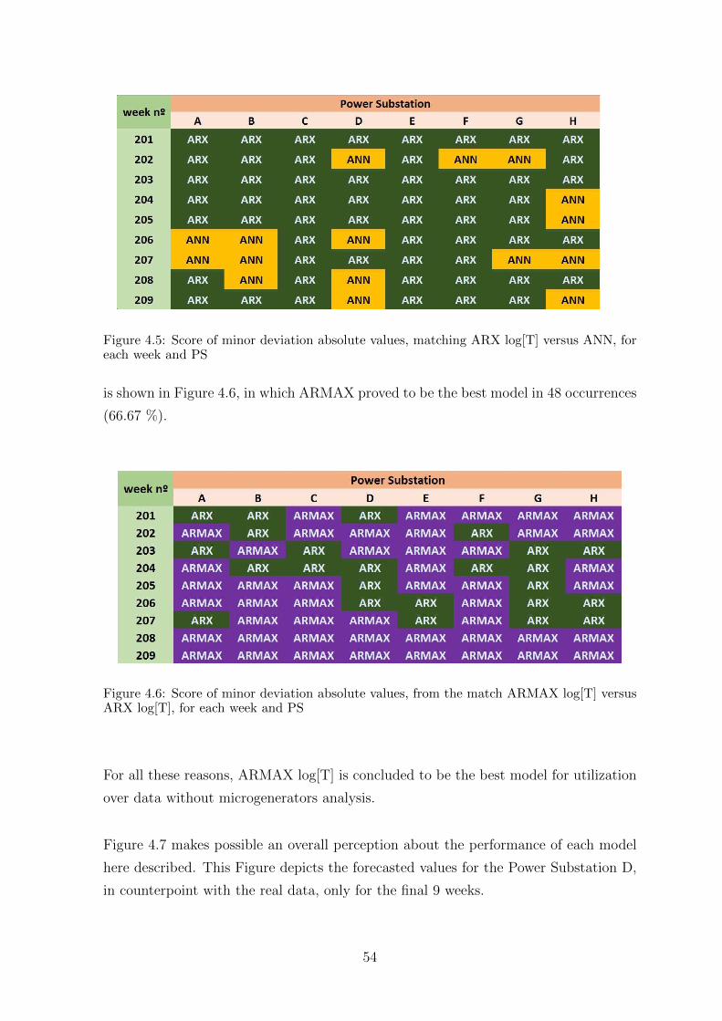
Figure 4.5: Score of minor deviation absolute values, matching ARX log[T] versus ANN, foreach week and PS
is shown in Figure 4.6, in which ARMAX proved to be the best model in 48 occurrences
(66.67 %).
Figure 4.6: Score of minor deviation absolute values, from the match ARMAX log[T] versusARX log[T], for each week and PS
For all these reasons, ARMAX log[T] is concluded to be the best model for utilization
over data without microgenerators analysis.
Figure 4.7 makes possible an overall perception about the performance of each model
here described. This Figure depicts the forecasted values for the Power Substation D,
in counterpoint with the real data, only for the final 9 weeks.
54

Figure 4.7: Measured data and forecast data for Power Substation D (3092), during the 9last weeks of 2004.
Curves from Fig. 4.7 do not illustrate continuous values, but rather discrete outcomes;
however, in order to make it more visually comprehensible, lines were designed to
connect the output values.
We perceive that forecast data from ARX and ARX log[T] curves are almost the
same, differing by a little offset; particularly in this PS, ARX seems to be nearer to
the measured data. However, ARX log[T] has been considered more successful over
the entire set of PSs, and therefore we can conclude that this PS in particular may
constitute an outlier with regards to ARX and ARX log[T]. Values from AR projections
are very close to ARX and ARX log[T], and like them, AR makes a peak value in the
5th week, as well as ARMAX and ANN.
However, ARMAX was the only model capable of forecasting the peak of the 8th week.
The ANN curve did it also, however, it was more likely to be a recuperation from the
erratic plunge occurred in the 7th week, where the measured data indeed get lower,
but not so sharply.
Another remark can be made upon the 4th week, where ARMAX apparently drifts
apart from the measured data. After this deviation, it lasts only 3 weeks to get the trend
again, whereas AR, ARX and ARX log[T] seem to present a very slower reaction. The
unstability of ANN is not observed among the AR models (AR, ARX and ARMAX).
Curves from Fig. 4.8 are now applied to the remaining Power Substations, in order to
enable a complete assessment of the prediction models over the entire set of PS.
55

Figure 4.8: Measured data and forecast data for Power Substations A, B, C, E, F, G and Hduring the 9 last weeks of 2004.
56

After concluding that ARMAX is the most suitable model for undertake forecasts, we
now illustrate the result of ARMAX predicitons for 2005 and 2006. Fig. 4.9 shows
curves for the 8 Power Substations, being blue lines for measured data and red lines
depicting ARMAX forecasts. Both years will be important for our analyses within the
next chapter, which will consider 2005 and 2006 forecasts.
4.2 Leipzig Map for the Power Substations
The main characteristics of each region is hereafter outlined, based on [52].
Power Station 1104 lies in the Meusdorf District, Southeast of Leipzig. This district
has a very low Demographic Density, and on average has 1.9 up to 2.0 inhabitants per
house. Population growth in this area is 9 % to 15 %. Circa 70 % of those residents
are economically active, and on average they think that their economic situation is
stagnated.
Power Station 1108 is located in in the Gohlis-Mitte District, Center of Leipzig. Power
Station 1109 lies in the Gohlis-Nord District, Center-North of Leipzig. Both districts
have high Demographic Densities, and on average both have 2.2 or more inhabitants per
house. Population growth for the two districts is between 9 % and 15 %. Circa 70 %
of Gohlis-Mitte residents are economically active, whereas this rate for Gohlis-Nord
District is 80%.
Power Station 3092 has place in the Schonefeld-Ost District, Center-Northeast of
Leipzig. Power Station 3219 lies in the Paunsdorf District, East of Leipzig. Both
districts have medium demographic densities. Population growth in Schonefeld-Ost
is 3 % to 9 %. In Paunsdorf, population growth is in the range from -3 % to 3 %.
Approximately 60 % residents are economically active, for both areas.
Power Station 3244 is located in the Heiterblick District, East of Leipzig. This district
has a medium Demographic Density, and on average has under 1.9 inhabitants per
house. Population growth in this area is negative, lower than -3 %. Circa 50 % of
those residents are economically active, and on average they think that their economic
situation is worsening.
57

Figure 4.9: ARMAX forecasted maximum electric power demands for 2005 and 2006, for everyPS: the blue line relates to measured data, whereas red lines describe ARMAX predictiondata. 58

Power Station 4012 lies in the Grunau Siedlung District, West of Leipzig. This district
has a high Demographic Density. Population growth in this area is 15 % or higher.
Circa 50 % of those residents are economically active. Power Station 4254 lies in the
Lausen Grunau District, West of Leipzig. This district has a very low Demographic
Density, and on average has under 1.9 inhabitants per house. Population growth in
this area is 9 % to 15 %. Circa 60 % of those residents are economically active, and on
average they think that their economic situation is improving.
Preparing the spatial analysis, Leipzig map is introduced, and the location of each one
of the 8 PS is signalized, as shown in Fig. 4.10.
Figure 4.10: Leipzig Map with the 8 Power Stations located [52].
59

Chapter 5 ENERGY DEMAND PREDICTION
INCLUDING RENEWABLE ENERGY GENERATION
Along the previous chapter, we studied the adequacy of the insertion of temperature
as an exogeneous variable, and we calculated na, nb, nc and nk so that we achieved
satisfactory auto-regressive models, as well as neural networks. These tasks were un-
dertaken in order to compare the several models each other, from which we concluded
ARMAX as the most suitable model in forecasting future maximum power demands,
given the quantity and conditions of power demand data.
In the current chapter, we evaluate the insertion of renewable sources into consumer
houses and buildings. The same 209 weeks maximum power demands (2001-2004) were
admitted as input data. We considered possible energetic incomes from for microgener-
ation, whose values are based on the power that the three sources can afford steadily, as
shown in Table 3.5. The three sources - RF, PV panels and electric eels - are supposed
to operate only over the last 157 weeks, which corresponds to the last three years -
2002, 2003 and 2004.
New values for maximum power demands are then obtained from the difference between
the realistic values and those coming from the renewable sources. These new set of
values will thus be adopted as another set of input data.
Given that during 2001 there is not yet input from the emergent sources, but only
during the 2002-2004 period, and given that these renewable sources come in the grid
progressively, we simulated new trends for the power demand values seen by each
PS. After that, we trained our ANN and adjust our ARMAX according to the weeks
between January 2001 until October 2004, and we have then evaluated the adaptation
ability of each method to forecast values for the 9 last weeks of 2004.
Figure 5.1 shows the underlying idea for characterization of input data. Let us say
we have the realistic power demand d1, and the apparent power demand is d2: d1 is
the electric power that a set of consumers spends on their activities, whereas d2 is the
effective electric burden that the PS of these consumers has to sustain. The difference
between d1 and d2 is microgeneration power Pµg. In the beginning of the process, d1
60
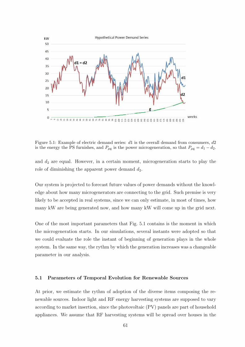
Figure 5.1: Example of electric demand series: d1 is the overall demand from consumers, d2is the energy the PS furnishes, and Pµg is the power microgeneration, so that Pµg = d1 − d2.
and d2 are equal. However, in a certain moment, microgeneration starts to play the
role of diminishing the apparent power demand d2.
Our system is projected to forecast future values of power demands without the knowl-
edge about how many microgenerators are connecting to the grid. Such premise is very
likely to be accepted in real systems, since we can only estimate, in most of times, how
many kW are being generated now, and how many kW will come up in the grid next.
One of the most important parameters that Fig. 5.1 contains is the moment in which
the microgeneration starts. In our simulations, several instants were adopted so that
we could evaluate the role the instant of beginning of generation plays in the whole
system. In the same way, the rythm by which the generation increases was a changeable
parameter in our analysis.
5.1 Parameters of Temporal Evolution for Renewable Sources
At prior, we estimate the rythm of adoption of the diverse items composing the re-
newable sources. Indoor light and RF energy harvesting systems are supposed to vary
according to market insertion, since the photovoltaic (PV) panels are part of household
appliances. We assume that RF harvesting systems will be spread over houses in the
61

same rate as the PV panels, given the probability of a person who recycles energy from
indoor light will also adopt RF recycling schemes.
5.1.1 Panels and antennas growing rates
The main task in this subsection is to project the number of antennas and panels that
people into a city will install in their homes. We suppose that the indicators of this
city and the general economic indicators of Brazil are alike. We divide this analysis
into the main trend and the oscillation that exists in the evolution of real data. We
calculate the main growing trend for PV panels and antennas, and we will apply over
them white noise values in order to simulate an inconstant measurement, as we observe
in the real world.
5.1.1.1 Main trend
According to Brazilian Telecommunication Regulatory Agency - ANATEL1, in 1990
there were about 667.000 cell phones in the country; in 1991, the number arose to 6.7
million (about 10 times) and, in the next year, the quantity achieved around 31.726
million cell phones. There is a logarithmic pattern within the increasing quantities
with regards to the beginning of the process. We depict the logarithm of the evolution
of cell phones in Brazil, considering the period from 1990 on, in Fig. 5.2(a). Fig.
5.2(b) illustrates the evolution of cable television users in the country, between 1993
and 2010, still according to data from Anatel.
Figure 5.2: (a) Increasing annual data for cell phones in Brazil since 1990; (b) Increasingannual data for cable TV in Brazil since 1993 (Anatel).
1In portuguese, Agencia Nacional de Telecomunicacoes - ANATEL
62
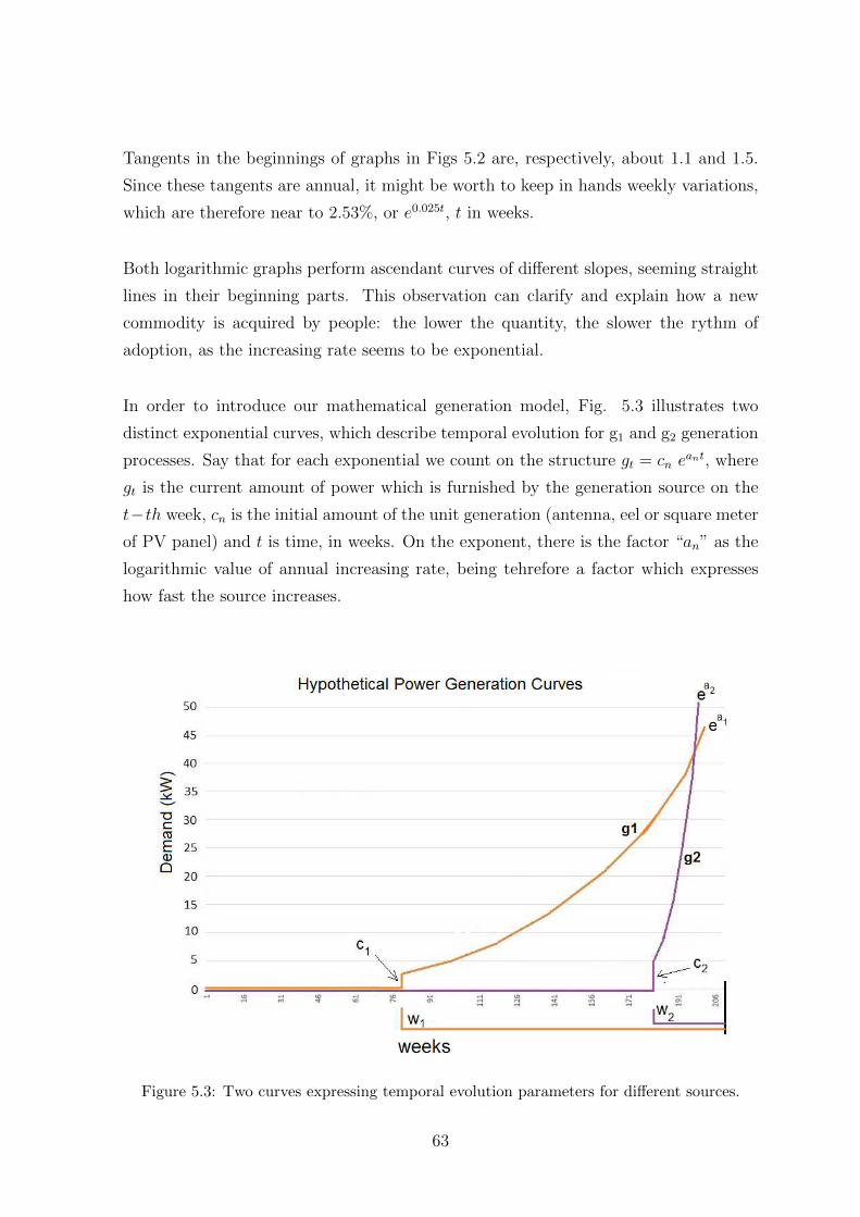
Tangents in the beginnings of graphs in Figs 5.2 are, respectively, about 1.1 and 1.5.
Since these tangents are annual, it might be worth to keep in hands weekly variations,
which are therefore near to 2.53%, or e0.025t, t in weeks.
Both logarithmic graphs perform ascendant curves of different slopes, seeming straight
lines in their beginning parts. This observation can clarify and explain how a new
commodity is acquired by people: the lower the quantity, the slower the rythm of
adoption, as the increasing rate seems to be exponential.
In order to introduce our mathematical generation model, Fig. 5.3 illustrates two
distinct exponential curves, which describe temporal evolution for g1 and g2 generation
processes. Say that for each exponential we count on the structure gt = cn eant, where
gt is the current amount of power which is furnished by the generation source on the
t−th week, cn is the initial amount of the unit generation (antenna, eel or square meter
of PV panel) and t is time, in weeks. On the exponent, there is the factor “an” as the
logarithmic value of annual increasing rate, being tehrefore a factor which expresses
how fast the source increases.
Figure 5.3: Two curves expressing temporal evolution parameters for different sources.
63

The initial amount cn is the quantity of the source in the instant it starts to generate
power, being arbitrated for each source through several simulation cases. Time t is
measured in weeks from the instant the respective source steps in the grid. For instance,
if the first eel comes up in the system on the 23rd week, and the first solar PV panel
enters only on the 40th week, than in the 50th week we have t1 = 27 for eels generation,
but t2 = 10 for solar panels.
5.1.1.2 Determining a, a better exponent of e
Say Mpv is the number of square meter (m2) of PV panels that people install in their
houses. In order to confer a higher accuracy to our analysis, we look for determining
a, the exponent of e, which is multiplied by c in the term [ceat]. Figure 5.4, from
Internatitional Energy Agency Photovoltaic Power System (IEA PVPS), year 2013,
depicts the evolution of grid-connected and off-grid PV systems from 1992 on in Japan,
country which has taken as an example for the analysis.
Figure 5.4: Evolution of grid-connected and off-grid PV panels, in MW (IEA PVPS), inJapan.
64
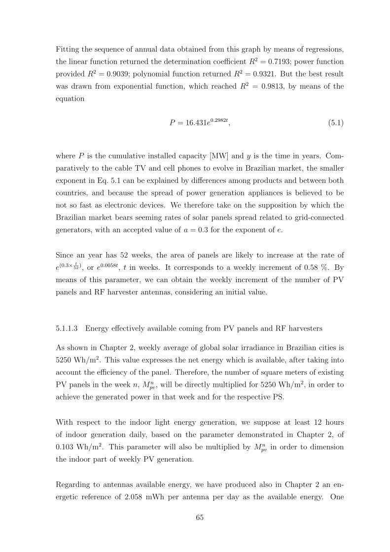
Fitting the sequence of annual data obtained from this graph by means of regressions,
the linear function returned the determination coefficient R2 = 0.7193; power function
provided R2 = 0.9039; polynomial function returned R2 = 0.9321. But the best result
was drawn from exponential function, which reached R2 = 0.9813, by means of the
equation
P = 16.431e0.2982t, (5.1)
where P is the cumulative installed capacity [MW] and y is the time in years. Com-
paratively to the cable TV and cell phones to evolve in Brazilian market, the smaller
exponent in Eq. 5.1 can be explained by differences among products and between both
countries, and because the spread of power generation appliances is believed to be
not so fast as electronic devices. We therefore take on the supposition by which the
Brazilian market bears seeming rates of solar panels spread related to grid-connected
generators, with an accepted value of a = 0.3 for the exponent of e.
Since an year has 52 weeks, the area of panels are likely to increase at the rate of
e(0.3×t
52), or e0.0058t, t in weeks. It corresponds to a weekly increment of 0.58 %. By
means of this parameter, we can obtain the weekly increment of the number of PV
panels and RF harvester antennas, considering an initial value.
5.1.1.3 Energy effectively available coming from PV panels and RF harvesters
As shown in Chapter 2, weekly average of global solar irradiance in Brazilian cities is
5250 Wh/m2. This value expresses the net energy which is available, after taking into
account the efficiency of the panel. Therefore, the number of square meters of existing
PV panels in the week n, Mnpv, will be directly multiplied for 5250 Wh/m2, in order to
achieve the generated power in that week and for the respective PS.
With respect to the indoor light energy generation, we suppose at least 12 hours
of indoor generation daily, based on the parameter demonstrated in Chapter 2, of
0.103 Wh/m2. This parameter will also be multiplied by Mnpv in order to dimension
the indoor part of weekly PV generation.
Regarding to antennas available energy, we have produced also in Chapter 2 an en-
ergetic reference of 2.058 mWh per antenna per day as the available energy. One
65

can notice that the total power obtained from indoor light and RF energy harvesting
reaches 0.105 Wh/m2, if we consider one antenna for each squared meter of PV panel.
Once we have obtained these values, we discount them from the original weekly data of
maximum consumption, in order to produce new values of power which is drawn from
the grid. The same step will be executed with regards to the power drawn by the eels.
5.1.2 Electric Eels Aquariums in the River
Let us suppose that the city hall is undertaking the duty of arising eels. The adminis-
trative staff has concluded that an acceptable growing rate of e1 a year for the baskets.
Each basket has area of 1m2 and contains one eel with 90 cm of size in average. Hence,
at the end of the first year, there will be around 108 eels generating energy; in the end
of the second year, the city will have approximately 296 eels distributed in 296 baskets
in the river. The reason for adopting an exponential serie of data lies on the need of
confering to eels the same treatment as to the other sources.
As demonstrated in Chapter 2, the available power in one hour during the peak is
Pe−peak = 24ne [W], where ne is the number of eels generating energy.
5.1.3 Unilateral white noise upon constant values: the k factor
Before we carry on, it is necessary to introduce a variable which provides the noise
character for temporal evolution of our sources. We suppose that unilateral white
noise values are indicated to confer oscillations to the previously calculated gt.
Consider an increasing series of discrete data y(n), as the weekly power demands. A
variable k assumes random instantaneous values between −A and A, being that A is
arbitrated; then, each outcome k multiplies the difference δ(n) between two consecutive
data y(n) and y(n+ 1), for each n. Each result is then summed to y(n). We establish
that y(n + 1) is not allowed to decrease in relation to y(n), and, therefore, occasional
negative values of δ(n) makes the current value y(n + 1) to be equal y(n). The term
“unilateral” comes from this criterion. The boundary value of k is chosen to simulate
variations which may overcome weekly increasing values, being rather an arbitrary
interval A. For a better comprehension of was just been said, Figure 5.5 is depicted.
66
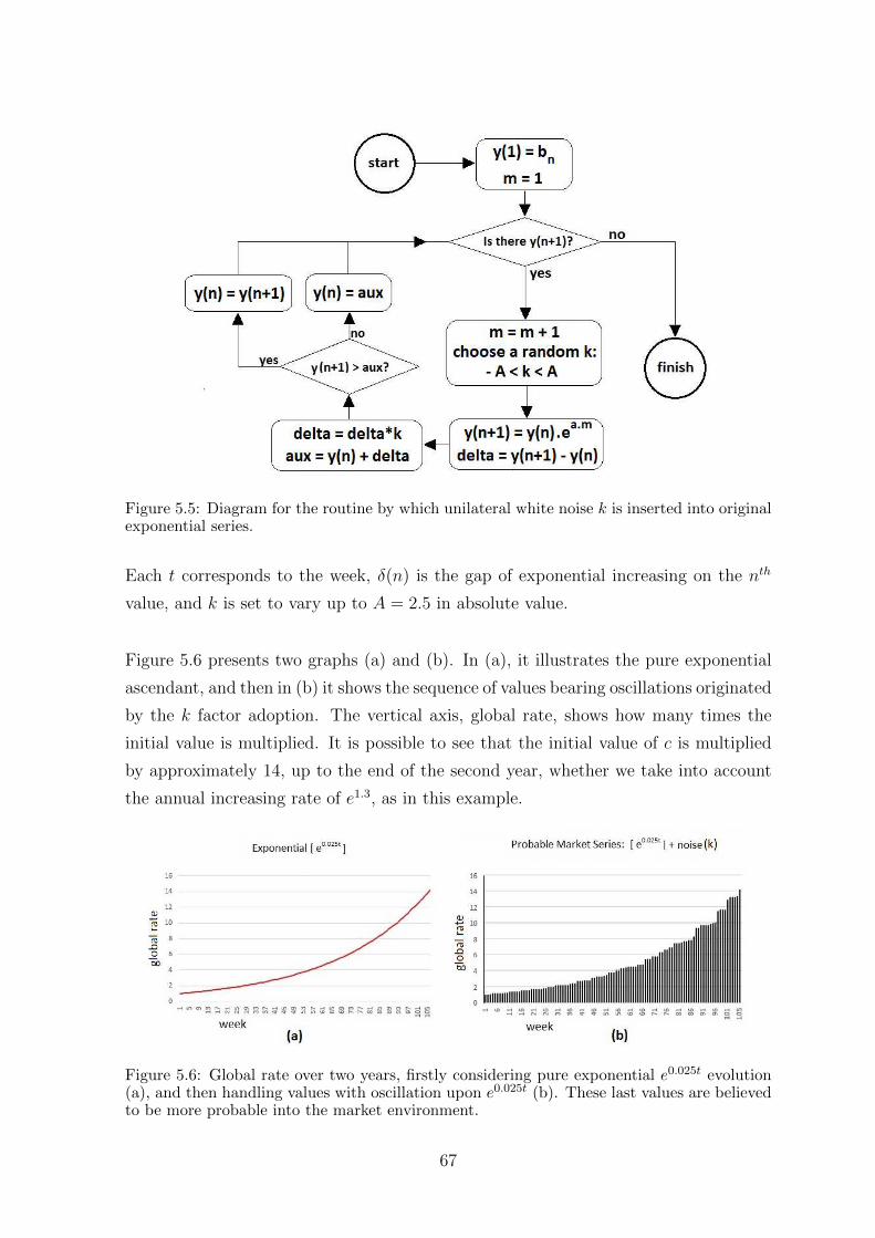
Figure 5.5: Diagram for the routine by which unilateral white noise k is inserted into originalexponential series.
Each t corresponds to the week, δ(n) is the gap of exponential increasing on the nth
value, and k is set to vary up to A = 2.5 in absolute value.
Figure 5.6 presents two graphs (a) and (b). In (a), it illustrates the pure exponential
ascendant, and then in (b) it shows the sequence of values bearing oscillations originated
by the k factor adoption. The vertical axis, global rate, shows how many times the
initial value is multiplied. It is possible to see that the initial value of c is multiplied
by approximately 14, up to the end of the second year, whether we take into account
the annual increasing rate of e1.3, as in this example.
Figure 5.6: Global rate over two years, firstly considering pure exponential e0.025t evolution(a), and then handling values with oscillation upon e0.025t (b). These last values are believedto be more probable into the market environment.
67
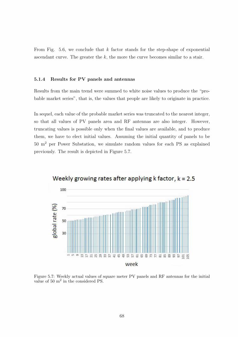
From Fig. 5.6, we conclude that k factor stands for the step-shape of exponential
ascendant curve. The greater the k, the more the curve becomes similar to a stair.
5.1.4 Results for PV panels and antennas
Results from the main trend were summed to white noise values to produce the “pro-
bable market series”, that is, the values that people are likely to originate in practice.
In sequel, each value of the probable market series was truncated to the nearest integer,
so that all values of PV panels area and RF antennas are also integer. However,
truncating values is possible only when the final values are available, and to produce
them, we have to elect initial values. Assuming the initial quantity of panels to be
50 m2 per Power Substation, we simulate random values for each PS as explained
previously. The result is depicted in Figure 5.7.
Figure 5.7: Weekly actual values of square meter PV panels and RF antennas for the initialvalue of 50 m2 in the considered PS.
68

5.2 Forecasting overall results considering power micro-generation values
Considering the parameters we have just presented, a brief analysis will be carried
out upon different values for each one of them. For an easier data comprehension, we
remember the definitions of the parameters as follows:
• w, in weeks, expresses the time during which the renewble emergent sources
will generate power, within the 209 weeks. For instance, if w = 52, then the
generators will step in at the 156th week, generating during 52 weeks until the
last week of the whole period;
• a, scalar, the annual exponent of e in the curve that illustrates quantities of each
source over time. Parameter a comes from market. We have resorted to Japanese
market data to arbitrate a as 0.3, in principle;
• k factor, which brings a noise pattern to be added to the original perfectly expo-
nential evolution for number of household appliances;
• c, in m2 of PV panels, units of antenas or eels: the amount of units of each source
when t starts to run, corresponding to the initial amount of units of a source in
the first week it generates energy.
We divide our analysis according to the solar panel utilization. The first case considers
that during sunny hours outdoor generation takes place, and we make use of the panels
for indoor light solely during evening and nights hours. In the second case, we avoid
outdoor generation, employing panels 24 hours inside buildings. The other two sources
- eels and RF antennas - will work in both cases, not depending on sun performance.
This division makes sense since solar panels yield 125 times more power in outdoor
environments, according to Table 3.5.
5.2.1 Solar PV Panels Generating Outdoor and Indoor
With solar panels generating in outdoor environments during day hours light, we de-
veloped simulations in two main cases: microgeneration running until 2 years, w going
from 35 until 80, and microgeneration running over more than two years, w starting
on 105 and going until 150.
69
5.2.1.1 Microgeneration Running Until 2 Years
We have firstly settled some different possible values for t, a and k: t assumed values
35, 50, 65 and 80; a assumed 0.3, 0.6, 0.9 and 1.2; and k was 1, 2 or 3. Since for t = 80
we have tested only a = 0.3 and a = 0.6, we have 42 results in hands.
Under these combinations, Table 5.1 gather results concerning to the MSE for each
method of the previous chapter, and also the best number of hidden layers for the
ANN structure, which has been used for ANN results.
For until one year of operation, the number of the best hidden layers for ANN system
becomes 5 for the first hidden layer, and 3 for the second one. There is not a precise
explication upon this fact, however we can remark that for the evaluated periods, both
quantities kept themselves practically constant.
Results for MSE are in accordance with has been shown in Chapter 4 about the order
of the most accurate model to the less accurate one. Table 5.1 shows that ANN MSE
stays above 4.0 in the most of time, being 3.8152 the minimum value in the entire set
of outcomes. The second less precise system, AR, had as its worst MSE the value of
2.7458, circa 7/10 of the best MSE for ANN. An overview let us notice that outcomes
for this table do not vary significantly.
With respect to the hypothesis of generation running during more than one year, we
have data from Table 5.2. We can behold the continuity with respect to the main
patterns of Table 5.1: ARMAX presenting the less errors, but, now, the best numbers
of neurons per layer in ANN system vary.
Some results are quite clear: the order by which methods are precise is the same as in
Chapter 4, i. e., ARMAX, ARX log[T], ARX, AR and ANN. In other words, the fact
of microgeneration starts to operate until 2 years from the end of 2004 does not breed
alterations on the quality of each model. One can observe that ARMAX is the only
method that reaches an MSE below 2.0, occurring on the input set w = 80, a = 0.6
and k = 2.
There is no longer an answer for the best couple of hidden layers into ANN mesh. One
possible explanation for it lies on time stretching: comprising more weeks far from the
end of the process, the exponential tendency has more time to appear. This tendency
70
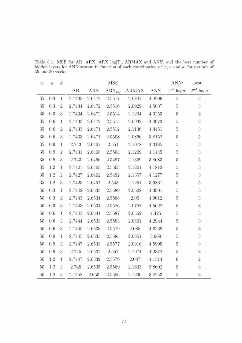
Table 5.1: MSE for AR, ARX, ARX log[T], ARMAX and ANN, and the best number ofhidden layers for ANN system in function of each combination of w, a and k, for periods of35 and 50 weeks.
w a k
35 0.3 1
35 0.3 2
35 0.3 3
35 0.6 1
35 0.6 2
35 0.6 3
35 0.9 1
35 0.9 2
35 0.9 3
35 1.2 1
35 1.2 2
35 1.2 3
50 0.3 1
50 0.3 2
50 0.3 3
50 0.6 1
50 0.6 2
50 0.6 3
50 0.9 1
50 0.9 2
50 0.9 3
50 1.2 1
50 1.2 2
50 1.2 3
MSE
AR ARX ARXlog ARMAX ANN
2.7433 2.6472 2.5517 2.0847 4.4209
2.7434 2.6472 2.5516 2.0929 4.5037
2.7434 2.6472 2.5514 2.1294 4.3253
2.7433 2.6472 2.5515 2.0932 4.4973
2.7433 2.6471 2.5512 2.1136 4.3451
2.7433 2.6471 2.5508 2.0866 3.8152
2.743 2.6467 2.551 2.1078 4.3185
2.7431 2.6468 2.5504 2.1209 4.1445
2.743 2.6466 2.5497 2.1399 3.8683
2.7427 2.6463 2.5503 2.1261 4.1812
2.7427 2.6462 2.5492 2.1357 4.1277
2.7423 2.6457 2.548 2.1251 3.9861
2.7442 2.6533 2.5589 2.0522 4.3901
2.7443 2.6534 2.5588 2.05 4.9612
2.7443 2.6534 2.5586 2.0757 4.5628
2.7443 2.6534 2.5587 2.0562 4.425
2.7444 2.6533 2.5583 2.0801 4.2944
2.7445 2.6533 2.5579 2.085 4.6239
2.7445 2.6533 2.5584 2.0851 3.969
2.7447 2.6533 2.5577 2.0916 4.5995
2.745 2.6532 2.557 2.1974 4.2372
2.7447 2.6532 2.5579 2.087 4.1514
2.745 2.6535 2.5569 2.1633 3.8602
2.7458 2.653 2.5556 2.1236 3.8253
ANN: best...
1st layer 2nd layer
5 3
5 3
5 3
5 3
5 3
5 5
5 3
5 3
5 5
5 3
5 3
5 5
5 3
5 3
5 3
5 3
5 3
5 3
5 3
5 3
5 3
6 2
5 3
5 3
71

Table 5.2: MSE for AR, ARX, ARX log[T], ARMAX and ANN, and the best number ofhidden layers for ANN system in function of each combination of w, a and k, for periods of65 and 80 weeks.
w a k
65 0.3 1
65 0.3 2
65 0.3 3
65 0.6 1
65 0.6 2
65 0.6 3
65 0.9 1
65 0.9 2
65 0.9 3
65 1.2 1
65 1.2 2
65 1.2 3
80 0.3 1
80 0.3 2
80 0.3 3
80 0.6 1
80 0.6 2
80 0.6 3
MSE
AR ARX ARXlog ARMAX ANN
2.7411 2.6491 2.5585 2.063 4.2143
2.7411 2.6491 2.5583 2.0622 3.9726
2.7411 2.6491 2.5582 2.0652 4.6301
2.741 2.649 2.5581 2.0671 4.027
2.7407 2.6485 2.5571 2.034 3.8377
2.7406 2.6482 2.5564 2.0991 5.8055
2.741 2.6489 2.5575 2.0848 4.3505
2.7409 2.6486 2.5563 2.0783 3.7064
2.7408 2.6486 2.5557 2.0424 3.7805
2.7412 2.6491 2.557 2.0449 3.6362
2.7404 2.6473 2.5537 2.0879 3.7963
2.7401 2.6464 2.5514 2.1454 3.7031
2.7432 2.6485 2.5629 2.0314 4.2768
2.7432 2.6484 2.5626 2.0421 3.7287
2.7433 2.6485 2.5626 2.0281 3.8034
2.7433 2.6485 2.5626 2.033 3.7119
2.7433 2.6486 2.5622 1.9882 4.0857
2.7429 2.6478 2.5609 2.0248 3.7552
ANN: best...
1st 2nd
4 4
5 6
5 6
5 4
5 4
5 6
5 6
4 6
4 4
3 4
3 4
4 4
6 2
5 6
3 4
3 2
6 2
4 4
72
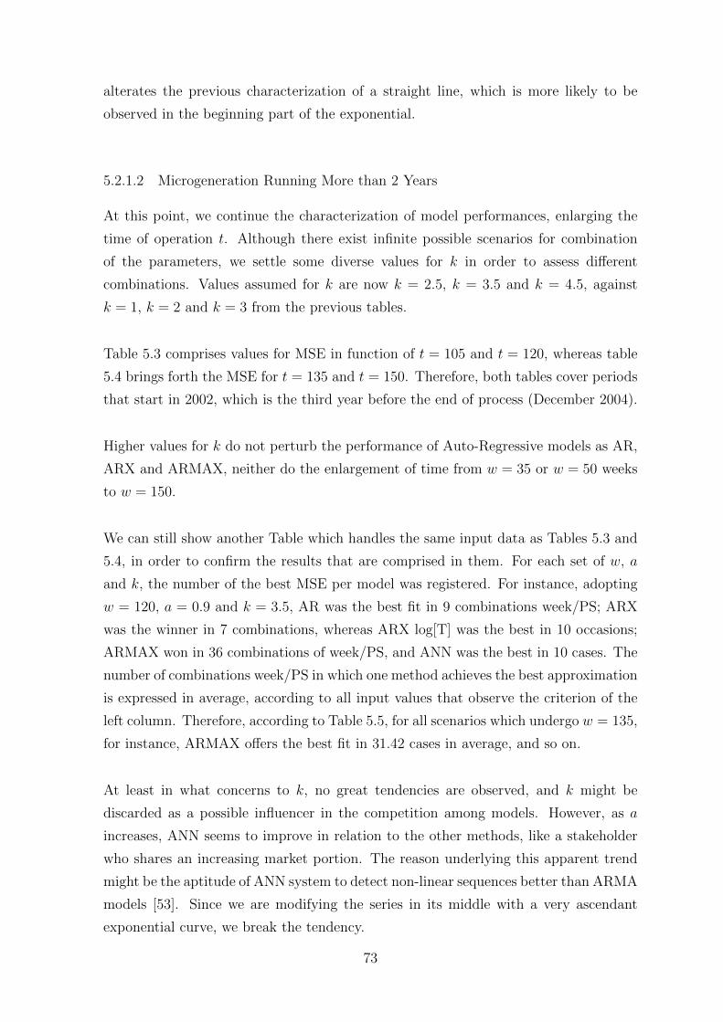
alterates the previous characterization of a straight line, which is more likely to be
observed in the beginning part of the exponential.
5.2.1.2 Microgeneration Running More than 2 Years
At this point, we continue the characterization of model performances, enlarging the
time of operation t. Although there exist infinite possible scenarios for combination
of the parameters, we settle some diverse values for k in order to assess different
combinations. Values assumed for k are now k = 2.5, k = 3.5 and k = 4.5, against
k = 1, k = 2 and k = 3 from the previous tables.
Table 5.3 comprises values for MSE in function of t = 105 and t = 120, whereas table
5.4 brings forth the MSE for t = 135 and t = 150. Therefore, both tables cover periods
that start in 2002, which is the third year before the end of process (December 2004).
Higher values for k do not perturb the performance of Auto-Regressive models as AR,
ARX and ARMAX, neither do the enlargement of time from w = 35 or w = 50 weeks
to w = 150.
We can still show another Table which handles the same input data as Tables 5.3 and
5.4, in order to confirm the results that are comprised in them. For each set of w, a
and k, the number of the best MSE per model was registered. For instance, adopting
w = 120, a = 0.9 and k = 3.5, AR was the best fit in 9 combinations week/PS; ARX
was the winner in 7 combinations, whereas ARX log[T] was the best in 10 occasions;
ARMAX won in 36 combinations of week/PS, and ANN was the best in 10 cases. The
number of combinations week/PS in which one method achieves the best approximation
is expressed in average, according to all input values that observe the criterion of the
left column. Therefore, according to Table 5.5, for all scenarios which undergo w = 135,
for instance, ARMAX offers the best fit in 31.42 cases in average, and so on.
At least in what concerns to k, no great tendencies are observed, and k might be
discarded as a possible influencer in the competition among models. However, as a
increases, ANN seems to improve in relation to the other methods, like a stakeholder
who shares an increasing market portion. The reason underlying this apparent trend
might be the aptitude of ANN system to detect non-linear sequences better than ARMA
models [53]. Since we are modifying the series in its middle with a very ascendant
exponential curve, we break the tendency.
73
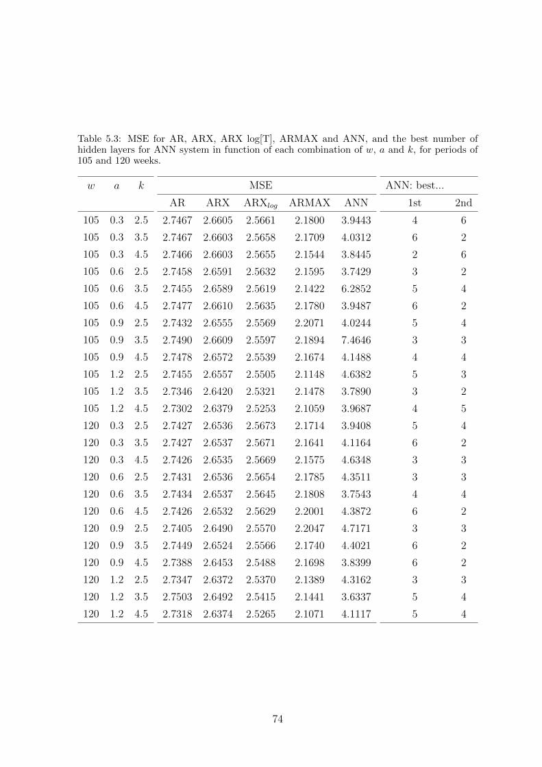
Table 5.3: MSE for AR, ARX, ARX log[T], ARMAX and ANN, and the best number ofhidden layers for ANN system in function of each combination of w, a and k, for periods of105 and 120 weeks.
w a k
105 0.3 2.5
105 0.3 3.5
105 0.3 4.5
105 0.6 2.5
105 0.6 3.5
105 0.6 4.5
105 0.9 2.5
105 0.9 3.5
105 0.9 4.5
105 1.2 2.5
105 1.2 3.5
105 1.2 4.5
120 0.3 2.5
120 0.3 3.5
120 0.3 4.5
120 0.6 2.5
120 0.6 3.5
120 0.6 4.5
120 0.9 2.5
120 0.9 3.5
120 0.9 4.5
120 1.2 2.5
120 1.2 3.5
120 1.2 4.5
MSE
AR ARX ARXlog ARMAX ANN
2.7467 2.6605 2.5661 2.1800 3.9443
2.7467 2.6603 2.5658 2.1709 4.0312
2.7466 2.6603 2.5655 2.1544 3.8445
2.7458 2.6591 2.5632 2.1595 3.7429
2.7455 2.6589 2.5619 2.1422 6.2852
2.7477 2.6610 2.5635 2.1780 3.9487
2.7432 2.6555 2.5569 2.2071 4.0244
2.7490 2.6609 2.5597 2.1894 7.4646
2.7478 2.6572 2.5539 2.1674 4.1488
2.7455 2.6557 2.5505 2.1148 4.6382
2.7346 2.6420 2.5321 2.1478 3.7890
2.7302 2.6379 2.5253 2.1059 3.9687
2.7427 2.6536 2.5673 2.1714 3.9408
2.7427 2.6537 2.5671 2.1641 4.1164
2.7426 2.6535 2.5669 2.1575 4.6348
2.7431 2.6536 2.5654 2.1785 4.3511
2.7434 2.6537 2.5645 2.1808 3.7543
2.7426 2.6532 2.5629 2.2001 4.3872
2.7405 2.6490 2.5570 2.2047 4.7171
2.7449 2.6524 2.5566 2.1740 4.4021
2.7388 2.6453 2.5488 2.1698 3.8399
2.7347 2.6372 2.5370 2.1389 4.3162
2.7503 2.6492 2.5415 2.1441 3.6337
2.7318 2.6374 2.5265 2.1071 4.1117
ANN: best...
1st 2nd
4 6
6 2
2 6
3 2
5 4
6 2
5 4
3 3
4 4
5 3
3 2
4 5
5 4
6 2
3 3
3 3
4 4
6 2
3 3
6 2
6 2
3 3
5 4
5 4
74

Table 5.4: MSE for AR, ARX, ARX log[T], ARMAX and ANN, and the best number ofhidden layers for ANN system in function of each combination of w, a and k, for periods of135 and 150 weeks.
w a k
135 0.3 2.5
135 0.3 3.5
135 0.3 4.5
135 0.6 2.5
135 0.6 3.5
135 0.6 4.5
135 0.9 2.5
135 0.9 3.5
135 0.9 4.5
135 1.2 2.5
135 1.2 3.5
135 1.2 4.5
150 0.3 2.5
150 0.3 3.5
150 0.3 4.5
150 0.6 2.5
150 0.6 3.5
150 0.6 4.5
150 0.9 2.5
150 0.9 3.5
150 0.9 4.5
150 1.2 2.5
150 1.2 3.5
MSE
AR ARX ARXlog ARMAX ANN
2.7395 2.6420 2.5602 2.2294 3.9212
2.7392 2.6419 2.5598 2.2513 3.6218
2.7396 2.6421 2.5598 2.2319 3.8483
2.7386 2.6413 2.5572 2.2570 4.1820
2.7383 2.6410 2.5558 2.2665 4.2890
2.7390 2.6407 2.5541 2.2333 4.3708
2.7422 2.6398 2.5504 2.1660 18.331
2.7373 2.6370 2.5425 2.2028 5.7739
2.7455 2.6400 2.5454 2.1787 4.3471
2.7033 2.5959 2.4927 2.1318 3.7499
2.7302 2.6314 2.5202 2.3369 4.9214
2.6764 2.5615 2.4500 2.0434 3.5608
2.7430 2.6447 2.5632 2.3016 3.9518
2.7433 2.6450 2.5632 2.2988 3.8121
2.7428 2.6442 2.5623 2.3168 3.8483
2.7448 2.6458 2.5613 2.2833 4.0309
2.7455 2.6462 2.5603 2.2204 3.9102
2.7463 2.6466 2.5593 2.2066 3.8721
2.7379 2.6365 2.5445 2.2835 4.1765
2.7552 2.6512 2.5538 2.2943 4.3579
2.7345 2.6306 2.5317 2.2144 3.4395
2.7288 2.6254 2.5148 2.3137 4.2285
2.7268 2.6128 2.5047 2.1735 4.0368
ANN: best...
1st 2nd
6 2
5 4
6 2
6 2
4 4
5 3
4 4
2 6
4 2
3 2
4 2
3 2
6 2
6 5
6 2
6 2
6 2
4 2
6 2
4 2
4 6
4 2
4 2
75

Table 5.5: Number of cases in which a model achieves the best approximation, taking intoaccount all cases that obbey to the criterion on the left column.
Criterion
w = 105
w = 120
w = 135
w = 150
a = 0.3
a = 0.6
a = 0.9
a = 1.2
k = 2.5
k = 3.5
k = 4.5
Best Approximation Average Occurrences
AR ARX ARXlog ARMAX ANN
11.0000 7.0000 9.6667 31.4167 12.9167
9.91670 6.7500 9.0833 31.5833 14.6667
12.5000 9.5000 8.1667 29.1667 12.6667
12.3636 9.7273 8.8182 27.4545 13.6364
11.2500 8.9167 9.6667 29.5000 12.6667
11.0833 8.4167 8.5000 30.9167 13.0833
11.6667 7.8333 9.0833 29.6667 13.7500
11.7273 7.6364 8.4545 29.7273 14.4545
11.6875 8.3125 8.5625 30.0625 13.3750
11.1875 8.2500 9.7500 29.0000 13.8125
11.4000 8.0667 8.4667 30.8667 13.2000
Interestingly, when w is enhanced, ARMAX seems to lose accuracy. Nevertheless, in
its worst performance, which is 27.4545 combinations week/PS, for w = 150, ARMAX
overcomes ANN in two times. But this may arise the question: if we enlarged our
sample sufficiently, would ANN overcome the remaining models?
If we just raise the value of a, as we were doing, probably ANN could become a winner
in a given instant, but even that is not so determinable. However, Fig. 4.5 remembers
us that, even when two methods have the same number of greatest successes, one
can overcome the other one with a large advantage, whether in a direct confront. We
remind, from Fig. 4.5, that despite ANN and ARX log[T] have offered the same number
of best predictions, if we carry out a match between ARX log[T] and ANN, we obtain
ARX log[T] to prevail in 78% of the total matches.
5.2.2 Solar PV Panels Generating Only Indoor
Since in Fig. 4.7 we had illustrated the complete set of forecasts for Power Substation
D, now we assess, over the same PS, how the prediction behaves as we adopt only
indoor light as the PV panel source. The analysis will run upon Power Substation D
only for the sake of a fast comparison among the diverse methods, in face of different
initial quantities c for the sources and weekly increasing rates ea.
76
Firstly, we will consider w = 104, a = 2, initial units c = 50 for all sources, and k = 2.5.
Only indoor light will apply now. The result is depicted in Fig. 5.8.
Figure 5.8: New version for Fig. 4.6, now adopting w = 104, a = 2.0, k = 2.5 and c = 50.Realistic Data corresponds to Measured Data from Fig. 4.6.
AR curve has not changed its relative position to the output data. It is a very important
aspect since it confirms the series assembling: only components from past outputs are
present, and therefore they must accord only to y(t). ARX and ARX log[T] modify
a little their position in terms of offset, which is explainable due to the eXogeneous
input: ARX models are allowed to vary according other parameter which is different
of y(t). ARMAX model, which has still the Moving Average component, is now in a
different position, fairly adapted to the new position of y(t).
On the other hand, ANN reacts completely different, assuming rather a diverse shape
from that one of Fig. 5.6. The non-linearity of ANN black-box stands for its apparently
incomprehensible behavior.
Now setting w = 104, a = 1, initial units c = 80 for all sources, and k = 2.5, we try to
perceive if is there any consequence by lowering a and lifting c. The result is depicted
in Fig. 5.9. Only indoor light continues to apply.
In the example of Fig. 5.9, ARMAX has presented the best fit in 34 cases, against 16
from ANN and 10 from AR; ARX has achieved 7 best performances and ARX log[T]
reached just 5 best shots.
77
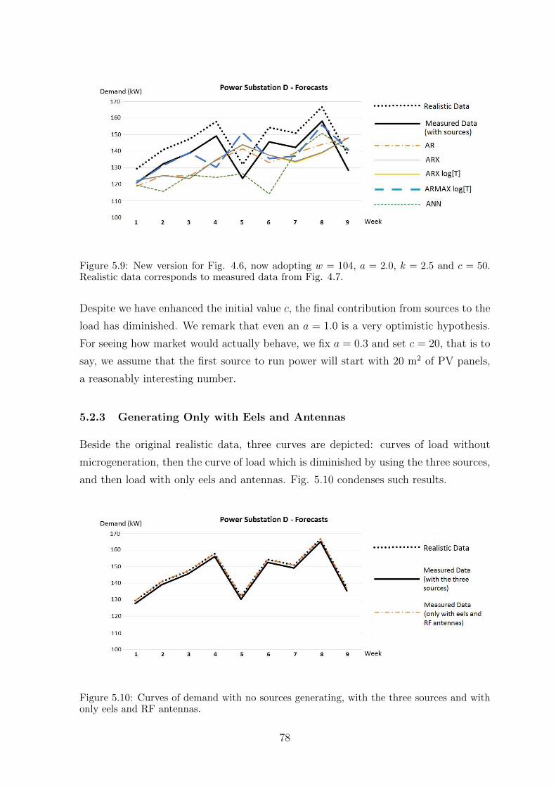
Figure 5.9: New version for Fig. 4.6, now adopting w = 104, a = 2.0, k = 2.5 and c = 50.Realistic data corresponds to measured data from Fig. 4.7.
Despite we have enhanced the initial value c, the final contribution from sources to the
load has diminished. We remark that even an a = 1.0 is a very optimistic hypothesis.
For seeing how market would actually behave, we fix a = 0.3 and set c = 20, that is to
say, we assume that the first source to run power will start with 20 m2 of PV panels,
a reasonably interesting number.
5.2.3 Generating Only with Eels and Antennas
Beside the original realistic data, three curves are depicted: curves of load without
microgeneration, then the curve of load which is diminished by using the three sources,
and then load with only eels and antennas. Fig. 5.10 condenses such results.
Figure 5.10: Curves of demand with no sources generating, with the three sources and withonly eels and RF antennas.
78

The difference between results without sources and with only antennas and eels are
very insignificant for the last 9 weeks. However, we should also test how would their
contribution be like in the end of 2006, and try to assess if they are also irrelevant in
the mean-term. Fig. 5.11 illustrates the tiny gap that antennas provide after 4 years
of participation, which barely overcomes 1 %. The initial quantity, in January 2002,
is 300 antennas, and the increasing rate is 1718% for year. A huge factor a of annual
expansion and a very high quantity at the beginning of the process c were not enough
to make antennas to become minimally feasible as a recycling energy source.
Figure 5.11: Antennas generating from January 2002, initial quantity of 300 antennas, in-creasing rate 172% for year, providing the tiny gap which is observed only in 2006 months.
With regards to the eels, Fig. 5.12 illustrates what happens if we choose a = 0.8 and
vary the initial quantity c, making c = 50 and c = 100, we notice that a gap is observed,
despite it is still very narrow. However, dealing with eels, we needed to resort to a
smaller initial amount of generator units. Moreover, the power availed by the eel may
be enhanced with further researches, since we have determined the lowest performance
in kWh. These points work towards not discarding eels as a feasible source yet. In
some cases, electric eels might show themselves as an advantageous source, but there is
still a plenty of necessary tests in order to probe their real energetic profit. The curve
79
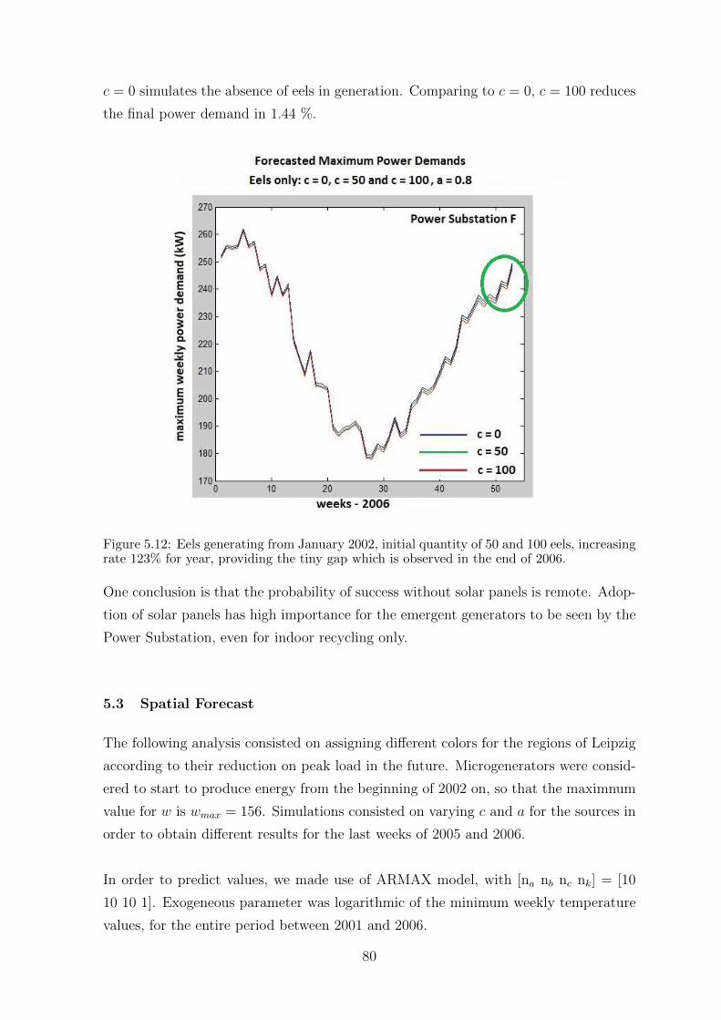
c = 0 simulates the absence of eels in generation. Comparing to c = 0, c = 100 reduces
the final power demand in 1.44 %.
Figure 5.12: Eels generating from January 2002, initial quantity of 50 and 100 eels, increasingrate 123% for year, providing the tiny gap which is observed in the end of 2006.
One conclusion is that the probability of success without solar panels is remote. Adop-
tion of solar panels has high importance for the emergent generators to be seen by the
Power Substation, even for indoor recycling only.
5.3 Spatial Forecast
The following analysis consisted on assigning different colors for the regions of Leipzig
according to their reduction on peak load in the future. Microgenerators were consid-
ered to start to produce energy from the beginning of 2002 on, so that the maximnum
value for w is wmax = 156. Simulations consisted on varying c and a for the sources in
order to obtain different results for the last weeks of 2005 and 2006.
In order to predict values, we made use of ARMAX model, with [na nb nc nk] = [10
10 10 1]. Exogeneous parameter was logarithmic of the minimum weekly temperature
values, for the entire period between 2001 and 2006.
80

Fig. 5.13 illustrates the code which assigns different colors to some reduction percent
values. These colors will be used to fill the 8 regions of Leipzig map in which the 8
Power Substations lie. Therefore, a certain combination of c and a will result in a peak
reduction which is classified in a visual way. The resulting peak load apply only to
the 5 weekdays; hence, Saturday and Sunday are not included. One can notice that
whether a district is filled in black, for instance, it means that the respective region
bears a PS whose peak load has been totally attended by the microgenerators. In
this situation, more than 100 % of the peak load is supplied by the emergent sources
between Monday and Friday, and the district might therefore export energy during the
peak.
Figure 5.13: Color codes for the weekly peak load relief percentages.
Let us establish ca and aa for antennas, ci and ai for PV panels indoor, co and ao for
PV panels outdoor, and ce and ae for the eels, where c is the initial amount of the
source and a is the logarithm of annual increase for it. The starting point for some
examples considers the following set of values: ca = 50, aa = 0.3; ci = 20, ai = 0.1;
co = 10, ao = 0.1; and ce = 100, ae = 0.2. Fig. 5.14 depicts the result. We notice that
only regions of Substations C and H have a relief in peak load corresponding to less
than 10 %. All the remaining regions lowered their peak consumptions in the range
10 % to 30 %. On the left part of each Figure we show the table of results and inputs,
and below the colors code is again depicted, as weel as the year corresponding to the
week which is predicted. Districts and Substations are understood to be related to the
same letter.
Setting all a = 0.2, we have now that all regions have peak allowances higher than
10 %, however none of them bearing economy of more than 30 % in the peak. Fig. 5.15
illustrates it. In the Fig. 5.15 and thereafter, figures also contain a row-table which
states some examples of the annual increasing rates depending on the value of a.
81

Figure 5.14: Simulation with ca = 50, aa = 0.3; ci = 20, ai = 0.1; co = 10, ao = 0.1; andce = 100, ae = 0.2, for the last week of 2005.
Figure 5.15: New simulation for scenario of Fig. 5.3, now setting all a = 0.2.
82

If the scenario of Fig. 5.15 endures until the end of 2006, the reduction of load along
the peak overcomes 30 % in districts where Substations A, D and E lie, as in Fig. 5.16:
Figure 5.16: Scenario of Fig. 5.3, this time for the last week of 2006.
Increasing the exponent of all sources to 0.3 and maintaining the analysis over the last
week of 2006, we can perceive the impact of a little enlargement of the exponent at
Fig. 5.17. Districts B, G and F reduce their weekdays peak load betwen 10 % and
30 %, whereas Substation A enhances their relief during the peak to more than 60 %.
Actually, peak load reduction for Substation A is 61.76 %, as the table in the left part
of this Figure lets us know.
Finally, elevating the initial amount only of the outdoor PV panels for co = 20, which
corresponds to doubling it, the impact over diminishing peak load, as depicted in
Fig. 5.18, is even more visible. Substations A, D and E achieves their complete energetic
sufficiency for weekdays peaks. Substations C and H goes to the next level of peak
load reduction, and so do Substations G, B and F.
The previous sequence of examples confirms some general ideas: the earlier the sources
are connected to the grid and the greater is the annual increase rate, the more relevant
is the impact of their energetic participation. The sequence of Figures also show that
different Power Substations avail themselves of the existing emergent power in different
83
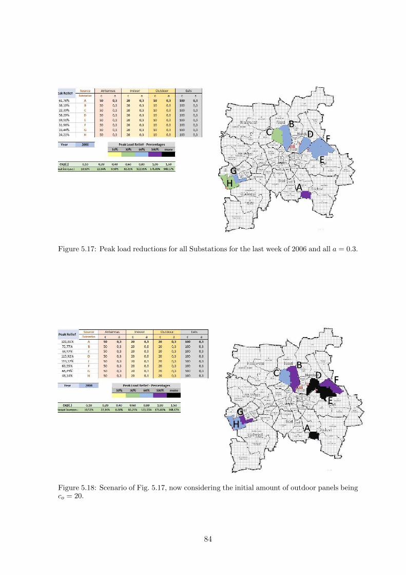
Figure 5.17: Peak load reductions for all Substations for the last week of 2006 and all a = 0.3.
Figure 5.18: Scenario of Fig. 5.17, now considering the initial amount of outdoor panels beingco = 20.
84

levels, as they present different average power demands. Finally, the increase of outdoor
panels area is much more relevant than any other source expansion.
There is a very plenty of possibilities in such test results, taking into account these
elements to vary. Therefore, Appendix C gathers many examples, in order to make
richer the analysis here initiated.
85

Chapter 6 CONCLUSIONS
Load prediction by means of temporal and spatial analysis is one of the most challenging
tasks addressed by public utilities. The assurance in sustaining load is not a trivial
task. The employment of correct data for information treatment techniques is each
time more needed in this realm. One factor that emphasizes this increasing necessity
is the change in the load behavior, given that new regulatory dispositions allow people
to produce their own energy. Such self energy generation occurs not only in Brazil, but
in many countries. The question arises: how does one accomplishes the best planning
method for load behavior prediction, and within an ever changing environment?
Along the present study, we aimed to offer an objective answer making use of prediction
techniques. In order to undertake any feasible analysis, reliable load data are the
first step. In Chapter 4 we have faced the problem of determining future values of
maximum power demands, with the best precision as possible, based on such data.
We have employed AR models in counterpoint with the ANN black-box. At prior, the
supposition was that ANN would not prevail since the set of mathematical resources at
disposal of AR models seems to be wider. Our first guess at this point was demonstrated
to be correct. ARMAX models attended the most of predicitons with the smallest
errors, and often the total set of best shots had a half of results coming from ARMAX.
It was also a recompense to find out that logarithmic temperature values yielded a fair
estimator of power demands. The weather question has strongly inspired us to consider
this parameter, but evidently other parameters should be investigated, as population
growth or GDP rates. It is true that most of these parameters were not available, but
we have produced an experience that proves exogeneous inputs to be welcome in order
to enhance explanation accuracy.
At the beginning of the process, the inclusion of three renewable sources - PV panels for
recycling, RF antennas and electric eels - made the work risky, once the real impact of
their generation was unknown. However, testing these different sources was important,
even because the assessment of traditional sources rises no longer very innovation.
New approaches are needed, and we should to seek for these new solutions whether
considering the little energy consumer, which is very sensitive to environmental issues
86

and therefore might adopt nonstandard solutions. Moreover, we tried to demonstrate
that several other forms of energy generation are likely to come up all over the cities.
Future market dispositions must count on this possibility. For instance, electric eels to
be considered as novel source is something that might cause some strangeness in the
first moment, but solutions like this might appear in the future.
The recycling objectives concerning to RF antennas and indoor light are worth it for
two reasons. The first one, in order to probe the real generation power from such tiny
sources. But it is also important as a way of showing people how difficult generating
energy steadily and assuredly can be. Protests against large hydroelectric plants, for
instance, would be undermined if people knew exactly how electric markets work, or
how hard is to make 1 kW to arrive satisfactorily in our houses and buildings. We
do not take for grant that such day will arrive, but the spread of little sources, as the
three tiny sources exploited along this dissertation, could help people to win the lack
of information and to become more sensitive to infrastructure problems - that is the
best hypothesis.
The insertion of such renewable emergent sources leads us back to the grid system
prediction discussion. We faced to estimate if future power demands would “feel” the
presence of the three studied emergent sources. Indirectly, it would show us whether
these sources are likely to be worth it. We have concluded that the insertion of solar
PV panels are perceived by the system undoubtedly if these panels convert energy from
outdoor. Depending on the amount of initial panels and on the increasing rythm of
adoption by people, these panels can be a relevant source even when they are used
solely for harvesting energy from indoor environments.
Eletric eels would need to be hugely employed if we wanted them to furnish the min-
imum amount of energy to be seen by the grid. The generation by means of RF
recycling antennas is certainly not a feasible option, i. e., we can discard this third
way of generating power.
The insertion of different loads under diverse scenarios of Chapter 5 did not modify
the efficiency ranking observed in pure load forecasting of Chapter 4. ARMAX proved
to be the most accurate model, and in the second position we counted on either AR
or ARX log[T], both disputing this second position, with a little advantage for ARX
log[T]. Again, the consideration of logarithmic values for temperature came up as a
good decision, since the performances of ARX fell short of the ones from ARX log[T].
87

All over this study, ANN system figured almost always as a sub-optimal forecasting
model. It was a meaningful perception because it was consistently observed in both
Chapters 4 and 5. Therefore, it allows us to conclude that, in the presence of Box
& Jenkins models, ANN is not likely to provide the best approximations. One might
say that 209 serial data are not a very large amount of information, and expanding
it would lead us to different results. However, many different combinations of input
parameters were undertaken in the present work. Only on the boundary of situations,
as elevating disproportionately one of the parameters, we beheld the improvement of
ANN performance. Even in such cases, ANN was not the best one.
We conclude that ARMAX is the best model for predicting load evolution, considering
or not energy furnished from power sources, while such sources consider renewable
solutions in the many diverse range of small power values. The prevalence of ARMAX,
ARX log[T] and AR models remained constant with over several situations, which
demonstrates the roubstness of these systems in the realm of time series predicition.
88

OWN PUBLICATIONS
[1∗] J. Milanezi Junior, J. P. C. L. da Costa, M. A. M. Marinho, R. S. Ferreira Junior,
E. P. de Freitas, “Arranjo e Metodo para Geracao de Energia Eletrica por meio de
Enguias Dispostas em Aquario”, Patent Pending in INPI, Process BR 10 2013 011210
0.
[2∗] J. Milanezi Junior, R. S. Ferreira Junior, J. P. C. L. da Costa, M. A. M. Mar-
inho, R. A. Shayani, R. T. de Sousa Junior, “Energy Harvesting Photovoltaic System
to Charge a Cell Phone in Indoor Environments”, IEEE International Conference on
Composite Materials and Renewable Energy Applications, Sousse, Tunisia, January
2014.
[3∗] J. Milanezi Junior, J. P. C. L. da Costa, M. A. M. Marinho, R. S. Ferreira Junior,
, R. A. Shayani, R. T. de Sousa Junior, “Sistema Fotovoltaico de Captacao de Energia
para Carga de Aparelhos Celulares em Ambientes Fechados”, V Congresso Brasileiro
de Energia Solar, Recife, Brazil, April 2014.
89

REFERENCES
[1] Agencia Nacional de Energia Eletrica, “Atlas de Energia Eletrica do Brasil”, 3a
edicao. Brasılia: Aneel, 2008.
[2] British Petroleum, “Statistical Review 1951-2011”, available in http://www.bp.com/
en/global/corporate/about-bp/energy-economics/statistical-review-of-world-energy-20
13/statistical-review-1951-2011.html
[3] http://www.wikienergia.pt/∼ edp/index.php?title = Intensidade energ%C3%A9tica,
websiteretrievedinFebruary21st 2014
[4] Brazilian Energy Balance 2013, Year 2012 / Empresa de Pesquisa Energetica Rio
de Janeiro: EPE, 2013.
[5] A. Al-Khayari, H. Al-Khayari, S. Al-Nabhani, M. M. Bait-Suwailam, and Z. Nadir,
“Design of an Enhanced RF Energy Harvesting System for Wireless Sensors”, 2013
IEEE GCC Conference and exhibition, November 17-20, 2013, pp. 479-482
[6] K. K. A. Devi, Norashidah Md.Din, C .K. Chakrabarty, and S. Sadasivam, “Design
of an RF - DC Conversion Circuit for Energy Harvesting”, IEEE International Con-
ference on Electronics Design, Systems and Applications (ICEDSA), 2012, pp. 156-161.
[7] M. Pinuela, P. D. Mitcheson, and S. Lucyszyn, “Ambient RF Energy Harvesting in
Urban and Semi-Urban Environments”, IEEE Transactions on Microwave Theory and
Techniques, Vol. 61, No. 7, July 2013, pp. 2715-2726.
[8] J. Paradiso and T. Starner, “Energy scavenging for mobile and wireless electronics”,
Pervasive Computing, Vol.4, No.1, pp. 18-27, JanMar 2005.
[9] H. Nishimoto, Y. Kawahara, T. Asami, “Prototype Implementation of Ambient
90

RF Energy Harvesting Wireless Sensor Networks”, IEEE SENSORS 2010 Conference,
pp. 1282-1287.
[10] M. Ali, L. Albasha, and N. Qaddoumi, “RF Energy Harvesting for Autonomous
Wireless Sensor Networks”, 8th International Conference on Design and Technology of
Integrated Systems in Nanoscale Era (DTIS), IEEE, 2013, pp. 78-81.
[11] M. Mi, “Analysis, Design, and Optimization of Antennas on CMOS Integrated
Circuits for Energy Harvesting Applications”, Dept. of Electrical Engineering, Uni.
Of Pittsburgh, 2003.
[12] C. A. Balanis, “Antenna theory: analysis and design”, John Wiley and Sons, 1997.
[13] Harry Ostaffe, “RF Energy Harvesting Enables Wireless Sensor Networks”, avail-
able in (http://www.sensorsmag.com/sensors-mag/rfenergy-harvesting-enables-wireless-
sensor-networks-6175), 2009.
[14] H. Jabbar, Y. S. Song, and T. T. Jeong, “RF Energy Harvesting System and
Circuits for Charging of Mobile Devices”, IEEE Transactions on Consumer Electron-
ics, Vol. 56, No. 1, February 2010, pp. 247-253.
[15] C. Mikeka, H. Arai, A. Georgiadis, and A. Collado, “DTV band micropower RF
energy-harvesting circuit architecture and performance analysis”, in IEEE Int. RFID-
Technol. Appl. Conf., 2011, pp. 561-567.
[16] H. J. Visser, and R. J. M. Vullers, “RF Energy Harvesting and Transport for
Wireless Sensor Network Applications: Principles and Requirements”, Proceedings of
the IEEE, Vol. 101, No. 6, June 2013, pp. 1410-1423.
[17] H. J. Visser, A. C. F. Reniers, and J. A. C. Theeuwes, “Ambient RF energy
scavenging: GSM and WLAN power density measurements”, in Proc. Eur. Microw.
Conf., Amsterdam, The Netherlands, 2008, pp. 721-724.
[18] T. Ungan, and L. M. Reindl, “Concept for Harvesting Low Ambient RF-Sources for
Microsystems”, http://www.imtek.de/content/pdf/public/2007/powermems 2007 pa
per ungan.pdf, accessed in 20th March 2010.
91
[19] Yan, H., Macias, J.G., Montero, Akhnoukh, A., De Vreede, L.C.N. and Burghartz,
J.N.: “An Integration scheme for RF Power harvesting”, Proc. STW Annual Workshop
on Semiconductor Advances for Future Electronics and Sensors, Veldhoven, Nether-
lands, November 2005, pages 64-66.
[20] J. Wang, L. Dong and Yuzhuo, Fu, “Modeling of UHF voltage multiplier for
radio-triggered wakeup circuit”, International Journal of Circuit Theory and Applica-
tion, 2010, DOI: 10.1002/cta.692.
[21] N. Barreca, H. M. Saraiva, P. T. Gouveia, J. Tavares, L. M. Borges, F. J. Velez,
C. Loss, R. Salvado, P. Pinho, R. Goncalves, N. B. Carvalho, R. Chavez-Santiago, and
I. Balasingham, “Antennas and Circuits for Ambient RF Energy Harvesting in Wire-
less Body Area Networks”, IEEE 24th International Symposium on Personal, Indoor
and Mobile Radio Communications: Fundamentals and PHY Track, 2013, pp. 532-537.
[22] https://en.wikipedia.org/wiki/DBm, website retrieved in February 21st 2014
[23] Q. I. Ali, “Design and implementation of a mobile phone charging system based
on solar energy harvesting”, in: EPC-IQ 2010, 2010, pp. 264-267.
[24] Y. Afsar, J. Sarik, M. Gorlatova, G. Zussman, I. Kymissis, “Evaluating photo-
voltaic performance indoors”, in: 2012 38th IEEE Photovoltaic Specialists Conference
(PVSC), 2012, pp. 1948-1951.
[25] M. Gorlatova, A. Wallwater, G. Zussman, “Networking low-power energy harvest-
ing devices: Measurements and algorithms”, in: 2011 Proceedings IEEE INFOCOM,
2011, pp. 1602-1610.
[26] A. S. Weddell, G. V. Merrett, , B. M. Al-Hashimi, “Ultra low-power photovoltaic
MPPT technique for indoor and outdoor wireless sensor nodes”, in: Design, Automa-
tion and Test in Europe Conference and Exhibition (DATE), 2011, 2011, pp. 14.
[27] H. Yu, Q. Yue, H. Wu, “Power management and energy harvesting for indoor
photovoltaic cells system”, in: 2nd International Conference on Mechanic Automation
and Control Engineering (MACE), 2011, pp. 521-524.
[28] C. Carvalho, J. P. Oliveira, N. Paulino, “Survey and analysis of the design issues
92
of a low cost micro power DC-DC step up converter for indoor light energy harvesting
applications”, in: 2012 Proceedings of the 19th International Conference Mixed Design
of Integrated Circuits and Systems (MIXDES), 2012, pp. 455-460.
[29] A. Somov, R. P. C. C. Ho, J. W. Evans, P. K.Wright, “Printed electrochemi-
cal capacitors for energy scavenging sensor networks”, in: Networked Sensing Systems
(INSS), 9th International Conference on, 2012, pp. 16.
[30] D. S. Ha, “Small scale energy harvesting - principles, practices and future trends”,
in: 2011 IEEE 14th International Symposium on Design and Diagnostics of Electronic
Circuits and Systems (DDECS), 2011, pp. 11.
[31] L. Huang, W. Rieutort-Louis, Y. Hu, J. Sanz-Robinson, S. Wagner, J. C. Sturm, N.
Verma, “Integrated all-silicon thin-film power electronics on flexible sheets for ubiqui-
tous wireless charging stations based on solar energy harvesting”, in: 2012 Symposium
on VLSI Circuits (VLSIC), 2012, pp. 198-199.
[32] Y. K. Tan, S. K. Panda, “Energy harvesting from hybrid indoor ambient light
and thermal energy sources for enhanced performance of wireless sensor nodes”, IEEE
Transactions on Industrial Electronics 58 (2011), pp. 4424-4435.
[33] H. Yu, H. Wu, Y. Wen, “An ultra-low input voltage power management circuit
for indoor micro-light energy harvesting system”, in: Sensors, 2010 IEEE, pp. 261-264.
[34] K.-J. Park, S.-M. Kang, H. S. Kim, C.-W. Baek, T. K. Chung, “Energy scav-
enging system utilizing mems switch for power management”, Electronics Letters 48
(2012), pp. 948-949.
[35] N. J. Guilar, T. J. Kleeburg, D. R. Y. A. Chen, R. Amirtharajah, “Integrated
solar energy harvesting and storage”, IEEE Transactions on Very Large Scale Integra-
tion (VLSI) Systems 17 (2009) 627-637.
[36] http://batteryuniversity.com/learn/article/charging lithium ion batteries (Novem-
ber 2013).
[37] M. Green, “Design calculations for buck-boost converters”, Texas Instruments Inc.
93

[38] B. M. Hasaneen, A. A. E. Mohammed, “Design and simulation of DC-DC boost
converter”, Selected Works.
[39] R. Zilles, M. A. B. Galhardo, S. H. F. de Oliveira, W. N. Macedo, “Sistemas
Fotovoltaicos Conectados a Rede Eletrica”, Oficina de Textos, 1a edicao, p. 43.
[40] Instituto Nacional de Meteorologia (INMET) and Laboratorio de Energia Solar
- EMC/UFSC (LABSOLAR), “Atlas de Irradiacao Solar do Brasil”, Brasilia-DF, Oc-
tober 1998.
[41] C. Chagas, and A. Paes de Carvalho, Bioeletrogenesis - A Comparative Survey
of its mechanisms with particular emphasis on electric fishes. Elsevier, Amsterdam,
1961.
[42] A. B. Assuncao, H. O. Schwassmann, “Reproduction and Larval Development of
Electrophorus Electricus on Marajo Island”, Ichthyological Explor Freshwaters 6, 175-
184, 1995.
[43] http://pages.vassar.edu/magnes/advanced-electromagnetism-phys-341/daniel-pea
rlman/
[44] http://www.icb.ufmg.br/labs/lpf/1-11.html
[45] M. V. Brown, “The Electric Discharge of the Electric Eel”, IEEE Electrical Engi-
neering, February 1950.
[46] http://www.pisciculturafb.com.br/artigos08.htm
[47] www.mathworks.com/help/ident/ref/fpe.html?
[48] C. B. Xiao, X. D. Zhang, and Y. D. Li, “A New Method for AR Order Determi-
nation of an ARMA Process”, IEEE TRANSACTIONS ON SIGNAL PROCESSING.
VOL. 44, NO. II , NOVEMBER 1996, pp. 2900-2903.
[49] M. H. F. Rahiman, M. N. Taib, and Y. M. Salleh, “Black Box Modeling of Steam
Distillation Essential Oil Extraction System using ARMAX Structure”, IEEE Interna-
tional Conference on Intelligent and Advanced Systems 2007, pp. 1059-1062.
94
[50] https://en.wikipedia.org/wiki/Weber%E2%80%93Fechner law
[51] Y Li, “Perceptions of temperature, moisture and comfort in clothing during envi-
ronmental transients”, Ergonomics, Volume 48, Issue 3, 2005, pp. 234-248.
[52] Leipziger Statistik und Stadtforschung, “Strukturatlas Leipzig 03-04”, Leipzig,
March 2004.
[53] J. C. Lu, D. X. Niu, and Z. W. Jia, “A Study of Short-Term Load Forecasting
Based on ARIMA-ANN”, Proceedings of the 3rd International Conference on Machine
Learning and Cybemetics, Shanghai, 26-29 August 2004, pp. 3183-3187.
[54] A. M. da Silva, “Estudo de Modelos ARIMA com Variaveis Angulares para Uti-
lizacao na Perfuracao de Pocos Petrolıferos”, Master Degree Dissertation, Campina
Grande - PB, Brazil, July 2007.
[55] G. A. Martins, and J. S. da Fonseca, “Curso de Estatıstica”, Atlas, 6a edicao.
[56] M. I. S. Bezerra, “Apostila de Analise de Series Temporais”, Curso de Estatıstica,
available in http://people.ufpr.br/ lucambio/CE017/1S2010/5515941-Apostila-Series-
Temporais.pdf
[57] https://en.wikipedia.org/wiki/Autocorrelation
[58] G. Lindgren, H. Rootzen, and M. Sandsten, “Stationary stochastic processes, parts
of Chapters 2 and 6”, available in http://www.math.chalmers.se/ rootzen/fintid/station
ary120312.pdf
[59] https://pt.wikipedia.org/wiki/N%C3%BAmero normal
[60] https://pt.wikipedia.org/wiki/Pi#Irracionalidade e transcend.C3.AAncia de
[61] R. M. Gray, and L. D. Davisson, “An Introduction to Statistical Signal Process-
ing”, Cambridge University Press, 2004.
[62] K. Oliveira, and M. Viana, “Fundamentos da Teoria Ergodica”, IMPA, Brazil.
95

[63] S.M.Deckmann, and J. A. Pomilio, “Avaliacao da Qualidade da Energia Eletrica”,
available in http://www.dsce.fee.unicamp.br/ antenor/pdffiles/qualidade/b5.pdf
[64] E. Assuncao, “Controle Digital”, Unesp, 2013.
[65] L. Lennart, “System Identification: Theory for the User”, Prentice Hall, Engle-
wood Cliffs, New Jersey 07632, 1987.
[66] T. Soderstrom, “Prediction Error Methods”, Control Systems, Robotics and Au-
tomation, Volume V.
96

APPENDICES
97

Appendix A Stationary Processes
A.1 Discrete-Time Stochastic Processes
Random variables can be easily found in our all day such as body temperature, heart
beat and bus schedule in Brasilia. For instance, we can compute the average and the
variance of the heart beat of a person. In a certain period and later on we compute
these values for the same person, collecting a set of data. We can find the average
and variance in the first period. If we discover that values to the average and variance
in the second period remain constant, it is an indication that we handle a stationary
process. From this example, we can define a stationary random variable as a random
variable with constant statistical properties - in this example, average and variance.
From statistics, we know that with the probability density funcion (PDF) of a random
variable, we can determine all its moments. We denote the moments as the statistical
properties, where the first moment of random variable is the mean, the second moment
is the variance, the third moment is the skewness and the forth moment is the kurtosis.
However, to find the PDF of a random variable in order to compute the moments would
require a large number of samples. Moreover, usually stationarity is only observed in
some time periods of the random variable. If the period becomes too long, the random
variable becomes nonstationary.
Therefore, instead finding the PDF, or the probability mass function (PMF), whether
our variable is discrete, we only seek for determining the first and second moment of a
random variable, which requires much less samples than determining the PDF. Discrete
variables differ from the continuous variables according to the specification over time.
We refer to time t as being time, however, a series can bear data which are organized
according to another physical parameter, as volume, distance, etc [14]. If the set of
time instants can be enumerated, we have a variable which is discrete. In other words,
the variable is discrete if and only if the observations between two arbitrary moments
are countable. Diversely, in the continuous case, the random variable is defined for all
value of t ∈ R.
Discrete variables are the ones which interested us along this work, given that math-
ematical tools which were employed, as auto-regressive and moving average models,
98

presume the variables to be discrete. Therefore, the distribution probability function
to speak of is the PMF.
A discrete-time stochastic process is a succession of events whose numerical values are
not related each other by any apparent logic and, moreover, presents discrete values.
Suppose you are driving a car through the streets of a large city: the succession of the
last numers of the cars’ plaques you see in front of you is a completely random process,
which does not undergo any logical principle. That is an example of stochastic process,
given that those numbers are not predictable; in the best hypothesis, you can suppose,
after seeing many “5” repeatedly, that the next number will not be a “5”, but, even in
this case, there is still a probability you mistake your prediction.
On the other hand, deterministic variables are ruled by physical laws like montion
of bodies, propagation of waves and temperature variations of a body in a controlled
environment. For instance, imagine you are inside a train and that the constant speed
of the train is 100 km/h. Therefore, after one hour, you know that you will 100 km
far from the original point and after two hours, 200 km far from the origin, and so on.
Therefore, ceteris paribus, there is no uncertainty on the distance computation in such
example.
The successive observations may compose a time series u(n), where, for example, u(1) =
3, u(2) = 0, u(3) = 9, . . ., u(n) = 5, where n is the number of registered data or the
sampling period. If we sum all these values and divide it by n, we calculate the mean
of the series.
µ(n) = Eu[n] = u[n]. (A.1)
The expression limN→∞1N
∑Nn=1 u[n] holds for ergodic processes, if we consider n as the
number of instantaneous observations in the present moment. However, if we assign n
to be the number of sampled observations, and provided that u(n) are independent and
identically distributed (iid), this limit becomes equivalent to (A.1), due to the Large
Numbers Law [61].
The mean in (A.1) consists on the first statistical moment of the random variable.
As we have shown above, the lacking of the PMF is rather compensated by the the
moments of the variable. Stationary processes handle these moments instead of the
distribution probability functions, which are supposed to be inaccessible.
99
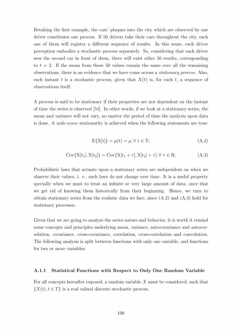
Retaking the first example, the cars’ plaques into the city which are observed by one
driver constitutes one process. If 50 drivers take their cars throughout the city, each
one of them will register a different sequence of results. In this sense, each driver
perception embodies a stochastic process separately. So, considering that each driver
sees the second car in front of them, there will exist other 50 results, corresponding
to t = 2. If the mean from these 50 values remain the same over all the remaining
observations, there is an evidence that we have come across a stationary process. Also,
each instant t is a stochastic process, given that X(t) is, for each t, a sequence of
observations itself.
A process is said to be stationary if their properties are not dependent on the instant
of time the series is observed [54]. In other words, if we look at a stationary series, the
mean and variance will not vary, no matter the period of time the analysis upon data
is done. A wide-sense stationarity is achieved when the following statements are true:
EX[t] = µ(t) = µ,∀ t ∈ T; (A.2)
CovX[t1],X[t2] = CovX[t1 + τ ],X[t2] + τ ],∀ τ ∈ R; (A.3)
Probabilistic laws that actuate upon a stationary series are independent on when we
observe their values, i. e., such laws do not change over time. It is a useful property
specially when we must to treat an infinite or very large amount of data, once that
we get rid of knowing them historically from their beginning. Hence, we turn to
obtain stationary series from the realistic data we face, since (A.2) and (A.3) hold for
stationary processes.
Given that we are going to analyze the series nature and behavior, it is worth it remind
some concepts and principles underlying mean, variance, autocovariance and autocor-
relation, covariance, cross-covariance, correlation, cross-correlation and convolution.
The following analysis is split between functions with only one variable, and functions
for two or more variables.
A.1.1 Statistical Functions with Respect to Only One Random Variable
For all concepts hereafter exposed, a random variable X must be considered, such that
X(t), t ∈ T is a real valued discrete stochastic process.
100

A.1.1.1 Mean
Mean value function (or expected value) is a well known concept: the sum of a set
of observations, divided by the number of these registers, provide us the mean of this
observed set, which is almost always a subset of a greater group. The mean of a random
vector X = [X1 X2 . . . Xn]T is defined as
E[X] = [EX1 EX2 . . . EXn]T (A.4)
The mean of a constant is the constant itself (A.5). Multiplying a random variable by
a constant α makes its mean be multiplyied by the same constant α (A.6) [55].
Eα = α (A.5)
EαX = αEX (A.6)
Supposing X(j) and X(j + τ) to be independent, the respective marginal PMFs are
equal to the joint PMF PXj, Xj+τ. In order to build covariance matrix, correlation
matrix and their respective “cross” versions, we introduce the deviation matrix, which
is given by
X− EX = dj =
X1 − EX1X2 − EX2
. . .
Xn − EXn
, (A.7)
which establishes an instantaneous value for the deviation vector on time; as in (A.7),
this vector is a list of the differences of each dimension of Xi to its mean. Although
it is a very frequent definition, the bibliography in many times uses another idea of
deviation vector, which involves successive values of deviation over time, taking an
unique dimension i of X into account:
di = [Xi,1 − EXi Xi,2 − EXi . . . Xi,j − EXi] , (A.8)
101
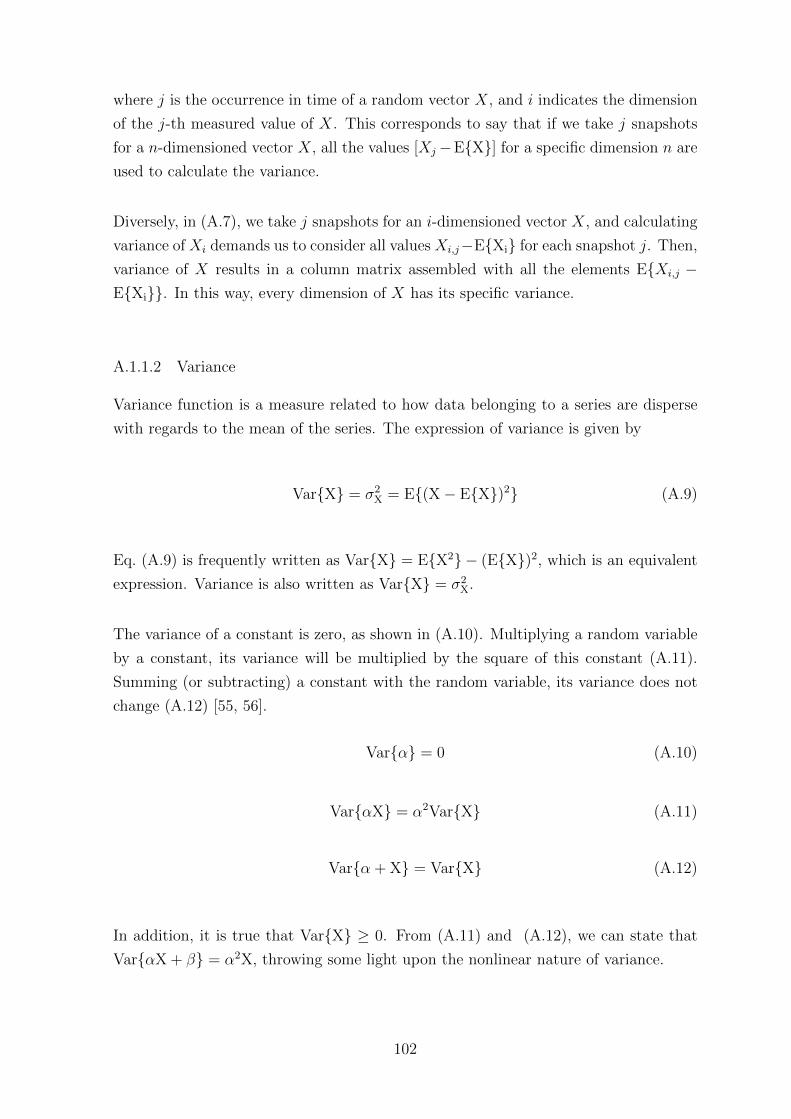
where j is the occurrence in time of a random vector X, and i indicates the dimension
of the j-th measured value of X. This corresponds to say that if we take j snapshots
for a n-dimensioned vector X, all the values [Xj−EX] for a specific dimension n are
used to calculate the variance.
Diversely, in (A.7), we take j snapshots for an i-dimensioned vector X, and calculating
variance of Xi demands us to consider all values Xi,j−EXi for each snapshot j. Then,
variance of X results in a column matrix assembled with all the elements EXi,j −EXi. In this way, every dimension of X has its specific variance.
A.1.1.2 Variance
Variance function is a measure related to how data belonging to a series are disperse
with regards to the mean of the series. The expression of variance is given by
VarX = σ2X = E(X− EX)2 (A.9)
Eq. (A.9) is frequently written as VarX = EX2 − (EX)2, which is an equivalent
expression. Variance is also written as VarX = σ2X.
The variance of a constant is zero, as shown in (A.10). Multiplying a random variable
by a constant, its variance will be multiplied by the square of this constant (A.11).
Summing (or subtracting) a constant with the random variable, its variance does not
change (A.12) [55, 56].
Varα = 0 (A.10)
VarαX = α2VarX (A.11)
Varα + X = VarX (A.12)
In addition, it is true that VarX ≥ 0. From (A.11) and (A.12), we can state that
VarαX + β = α2X, throwing some light upon the nonlinear nature of variance.
102

A.1.1.3 Autocorrelation Function
Say the random variable X has a known probability mass function given by f . The
autocorrelation function includes the operator “?” and is given by [57]
f ? f =∞∑
m=−∞f ∗(m)f(m+ n) (A.13)
Autocorrelation function provides X to “pass over” itself, such in an autoconvolution.
Actually, it is an autocorrelation, in the sense it is more likely to seem a cross-correlation
function rather than convolution, as we will show in the next section. Fig. A.1 provides
a visual comparison among the three functions here mentioned.
A.1.1.4 Correlation Matrix - correlating X(i) with X(i+ k), for different k
The deviation matrix di from Eq. (A.7) enables us to establish the relationship between
covariance and correlation, which will be explored in the next Section. Let L2di
be
L2di
= didTi =
n∑j=1
(xi,j − xi)2, (A.14)
such that xi,j is the value of X considering i as the dimension selected into Xn vector
and j as the order of the snapshot made over Xi. We also can see that Eq. (A.14)
contains a term L2di
which is proportional to the variance of Xi. Therefore we can write
as expression which is related to covariance, given by
didTk =
n∑j=1
(xi,j − xi)(xk,j − xk), (A.15)
where k describes another dimension of Xn (of course, both i and k must be less or
equal the dimension of X, n). If we want to know how redundant is information
brought by Xi and Xk, (A.15) can be rewritten as
didTk = LdiLdkcos(θi,k), (A.16)
103
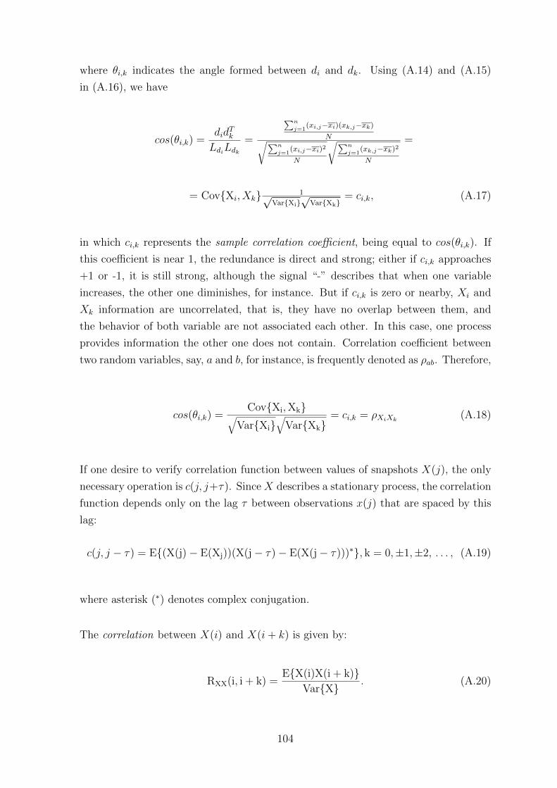
where θi,k indicates the angle formed between di and dk. Using (A.14) and (A.15)
in (A.16), we have
cos(θi,k) =did
Tk
LdiLdk=
∑n
j=1(xi,j−xi)(xk,j−xk)
N√∑n
j=1(xi,j−xi)2
N
√∑n
j=1(xk,j−xk)2
N
=
= CovXi, Xk 1√VarXi
√VarXk
= ci,k, (A.17)
in which ci,k represents the sample correlation coefficient, being equal to cos(θi,k). If
this coefficient is near 1, the redundance is direct and strong; either if ci,k approaches
+1 or -1, it is still strong, although the signal “-” describes that when one variable
increases, the other one diminishes, for instance. But if ci,k is zero or nearby, Xi and
Xk information are uncorrelated, that is, they have no overlap between them, and
the behavior of both variable are not associated each other. In this case, one process
provides information the other one does not contain. Correlation coefficient between
two random variables, say, a and b, for instance, is frequently denoted as ρab. Therefore,
cos(θi,k) =CovXi,Xk√
VarXi√
VarXk= ci,k = ρXiXk
(A.18)
If one desire to verify correlation function between values of snapshots X(j), the only
necessary operation is c(j, j+τ). Since X describes a stationary process, the correlation
function depends only on the lag τ between observations x(j) that are spaced by this
lag:
c(j, j − τ) = E(X(j)− E(Xj))(X(j− τ)− E(X(j− τ)))∗, k = 0,±1,±2, . . . , (A.19)
where asterisk (∗) denotes complex conjugation.
The correlation between X(i) and X(i+ k) is given by:
RXX(i, i + k) =EX(i)X(i + k)
VarX . (A.20)
104

By means of (A.20), we try to establish the relationship between different existing
i−dimensions the vector X(n). While (A.19) probes correlation over time, (A.20)
accomplishes the correlation between two diferent dimensions of X. Both types of
correlation are used in several analyses. Expression (A.19) is employed, for instance,
if one want to know if the variable of insterest has any seasonality or repetition; even
whether temporarily. On the other hand, (A.20) is more suitable if one intend to see
if X is over-dimensioned, since a positive answer indicates that two dimensons contain
the same information.
A.1.2 Statistical Functions with Respect to More than One Random Vari-
able
Two random variables X and Y must be considered now, being X(t), Y (t), t ∈ T two
real valued discrete stochastic processes. More than two variables might be considered,
however for the sake of simplicity we will include only X and Y in the following analysis.
Still talking about mean and variance, there are three interesting properties which have
not been yet exploited. Say we have a joint distribution of the above-mentioned two
random variables. The mean of their sum or difference equals the sum or difference of
their means (A.21), and the mean of the product of two independent random variables
is the product of their means (A.22):
EX + Y =∑i
∑j
(xi + yj)pxi, yj =
=∑i
∑j xipxi, yj+
∑i
∑j yjpxi, yj =
∑i xipxi+
∑j yjpyj =
= EX+EY (A.21)
EXY =∑i
∑j
xiyjpxi, yj =∑i
∑j
xiyjpxipyj =
=∑i xipxi
∑j yjpyj = EXEY (A.22)
The variance of the sum of two independent random variables is equal to the sum of
their respective variances (A.23):
VarX + Y = E[(X + Y)− (µX + µY)]2 = E[(X− µX) + (Y − µY)]2 =
105

= E(X - µX)2 − 2E(X− µX)(Y − µY)+ E(Y − µY)2 =
= VarX+VarY, (A.23)
since E(X − µX)(Y − µY) = CovX,Y = 0, given that X and Y are independent
[55, 56].
A.1.2.1 Covariance (or Auto-Covariance) Function
Covariance function between X and Y is defined as
CovX,Y = E(X− EX)(Y − EY) (A.24)
Eq. (A.24) may be written also as CovX,Y = EX,Y − EXEY. Covariance
between X and Y is also written as σXY .
Although its mathematic expression gives us a relatively simple statement, covariance
function is not a immediately comprehensible concept in the real world. In few words,
covariance expresses how much informations from X and Y are alike, taking into ac-
count the mean and absolute values of X and Y as relevant factors for the magnitude
of covariance [58].
A pure indicator of the existent “coincidence” between information coming from both
variables is rather the auto-correlation function, for the reason this function varies be-
tween -1 and 1 and brings in a directly geometric interpretation of in what degree the
overall values x(t) and y(t) are in accordance or, say, contain redundant information,
in the same way as in (A.18). Nevertheless, considering covariance might be advanta-
geous in certain circumstances. For instance, in Principal Components Analysis, if the
variances differ significantly each other, or if the measurement units are not compati-
ble, the principal components of covariance matrix will be dominated by the variables
which have the largest variances. This situation might be interesting given that usually
few principal components keep the most of the variance from original data. Therefore,
it consists on a situation wherein magnitudes of X and Y are important, or should be
strengthened.
If X and Y are independent, CovX,Y = 0. Among the properties listed below, some
other are understandable if one reminds variance properties.
106

Covα + βX, γ + κY = βκCovX,Y(A.25)
CovX,Y =VarX + Y − VarA − VarB
2(A.26)
CovX + Y,Z = CovX,Z+ CovY,Z (A.27)
CovX,X = VarX (A.28)
Covα,X = 0 (A.29)
One may use CovX(t),X(t + τ) = E(X(t)− EX(t))(X(t + τ)− EX(t + τ)) to
probe if X is stationary: whether CovX(t),X(t+τ) 6= 0, at least within the observed
period between t and t + τ , X bears dependence in time; X can, alternatively, be a
cicle-stationary random variable if, keeping τ constant, it continues to happen in all t
moments.
In matricial terms, (A.24) is now used to assemble covariance matrix of vector X, which
is here expressed as ΣX :
ΣX = E
X1 − EX1X2 − EX2
...
Xn − EXn
E[X1 − EX1 X2 − EX2 . . . Xn − EXn
](A.30)
Given that CovX,Y = 0 when X and Y are uncorrelated, we have EXEY =
EXY, and thus it is correct to state that
ΣX =
E(X1 − X1)(X1 − X1) E(X1 − X1)(X2 − X2) . . . E(X1 − X1)(Xn − Xn)E(X2 − X2)(X1 − X1) E(X2 − X2)(X2 − X2) . . . E(X2 − X2)(Xn − Xn)
......
. . ....
E(Xn − Xn)(X1 − X1) E(Xn − Xn)(X2 − X2) . . . E(Xn − Xn)(Xn − Xn)
(A.31)
107

where Xi = EXi. It is equivalent to
ΣX =
σ21 σ12 . . . σ1n
σ21 σ22 . . . σ2n
......
. . ....
σn1 σn2 . . . σ2n
(A.32)
According to (A.32), covariance matrix has, in its main diagonal, the variances of Xi
and, for i 6= j, the aij elements contain the covariances between Xi and Xj.
In the case our aim is to examinate time-lag behavior, we consider X(t) and X(t+τ) as
the variables of interest, and for them we can encounter the covariance matrix r(t, t+τ)
which is given by
rX(t, t+ τ) = Cov[X(t), X(t+ τ)] = E[X(t)X(t+ τ)]− E[X(t)]E[X(t+ τ)] (A.33)
Covariance between different values of X in time depend only on the lag of the obser-
vations, if X delineates a stationary process. Therefore, given a certain τ , Eq. (A.33)
holds for any value of τ . That is the reason why we rewrite it, obtaining
rX(τ) = CovX(t),X(t + τ) (A.34)
Covariance accepts commutation, i. e., CovX,Y = CovY,X. As the title of this
subsection let us know, covariance function is also named as auto-covariance function.
A.1.2.2 Cross-Covariance Function
The function
rX,Y (t, t+τ) = CovX(t),Y(t+τ) = EX(t)Y(t+τ)−EX(t)EY(t+τ) (A.35)
is called the cross-covariance function between X(t) and Y (t), being each variable
observed in instants of time spaced by τ . Cross-covariance function is a very important
tool in order to assemble the cross-covariance matrix: the elements out of the main
diagonal are cross-correlation function values. Writing rX,Y (t, t+τ) = σXY (τ), we have
108
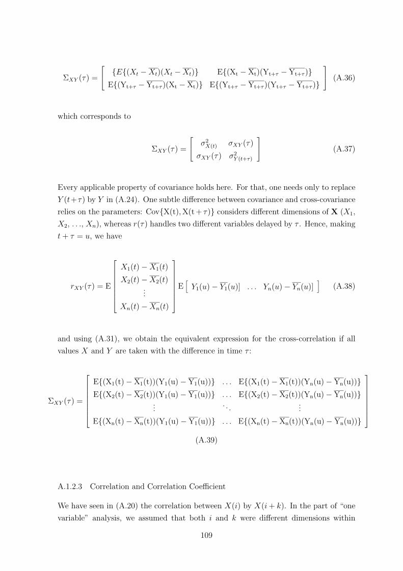
ΣXY (τ) =
E(Xt −Xt)(Xt −Xt) E(Xt − Xt)(Yt+τ − Yt+τ )E(Yt+τ − Yt+τ )(Xt − Xt) E(Yt+τ − Yt+τ )(Yt+τ − Yt+τ )
(A.36)
which corresponds to
ΣXY (τ) =
σ2X(t) σXY (τ)
σXY (τ) σ2Y (t+τ)
(A.37)
Every applicable property of covariance holds here. For that, one needs only to replace
Y (t+τ) by Y in (A.24). One subtle difference between covariance and cross-covariance
relies on the parameters: CovX(t),X(t + τ) considers different dimensions of X (X1,
X2, . . ., Xn), whereas r(τ) handles two different variables delayed by τ . Hence, making
t+ τ = u, we have
rXY (τ) = E
X1(t)−X1(t)
X2(t)−X2(t)...
Xn(t)−Xn(t)
E[Y1(u)− Y1(u)] . . . Yn(u)− Yn(u)]
](A.38)
and using (A.31), we obtain the equivalent expression for the cross-correlation if all
values X and Y are taken with the difference in time τ :
ΣXY (τ) =
E(X1(t)− X1(t))(Y1(u)− Y1(u)) . . . E(X1(t)− X1(t))(Yn(u)− Yn(u))E(X2(t)− X2(t))(Y1(u)− Y1(u)) . . . E(X2(t)− X2(t))(Yn(u)− Yn(u))
.... . .
...
E(Xn(t)− Xn(t))(Y1(u)− Y1(u)) . . . E(Xn(t)− Xn(t))(Yn(u)− Yn(u))
(A.39)
A.1.2.3 Correlation and Correlation Coefficient
We have seen in (A.20) the correlation between X(i) by X(i+ k). In the part of “one
variable” analysis, we assumed that both i and k were different dimensions within
109

X(n) vector, and hence i ≤ n, k ≤ n. Now we will check the correlation (function and
coefficient) between two different variables.
Correlation is simply the expected value of the product of two random variables:
EXY is the correlation between X and Y . However, there is another definition
which is much more utilized: the correlation coefficient, corresponding to the covari-
ance divided by the standard-deviations of each random variable, as in (A.40).
ρxy =CovX,Y√
VarXVarY=
E(X− EX)(Y − EY)σxσy
. (A.40)
Variables X and Y are supposed to not bear temporal lag in this case, i. e., X(τ) is
tested to be correlated to Y (τ) in the same instant τ they happen. Correlation function
provides more directly the indication of how two random variables (or measurements
of the only random variables) vary in the same way. We say “directly” because, on the
contrary of covariance, now the values are enclosed in the interval [-1, 1]. If ρxy = 0,
we know that the values are uncorrelated, i. e., there are not any information overlap
between X and Y . Expressions between (A.35) and (A.19) provide us to visualize that
mean, autocorrelation and autocovariance functions are related by
c(n, n− k) = r(n, n− k)− µ(n)µ(n− k)∗ (A.41)
for a random variable describing a stationary process.
A.1.2.4 Cross-Correlation
Since the term “cross” informs that there is at least one other random variable in the
function combined with a lag in time, say we have values of Xi and Yi which describe
two stationary processes. For cross-correlation, the lag is varied in order to promove
the “passage” of the values of a function over the other function values. For discrete
functions, in which we are interested, let us consider two PMFs given by f and g,
respectively to X and Y . The autocorrelation function includes the operator “?”, as
in (A.42).
f ? g =∞∑
m=−∞f ∗(m)g(m+ n) (A.42)
110
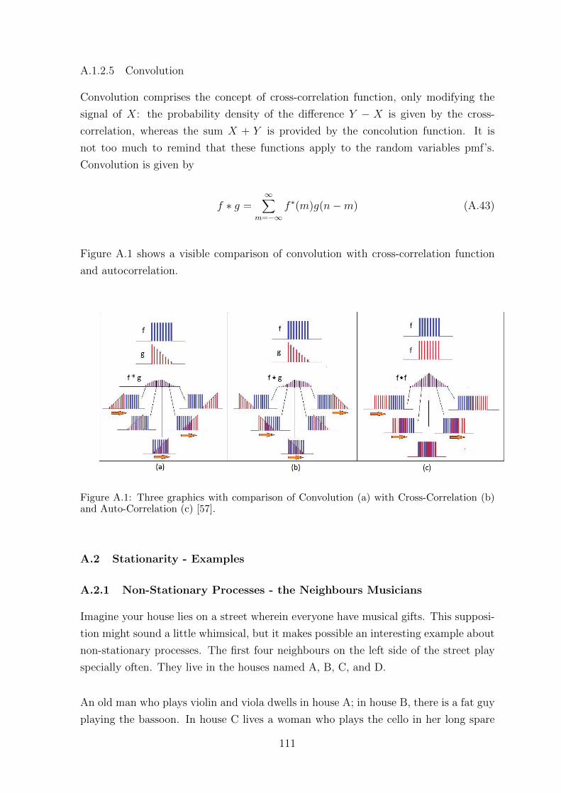
A.1.2.5 Convolution
Convolution comprises the concept of cross-correlation function, only modifying the
signal of X: the probability density of the difference Y − X is given by the cross-
correlation, whereas the sum X + Y is provided by the concolution function. It is
not too much to remind that these functions apply to the random variables pmf’s.
Convolution is given by
f ∗ g =∞∑
m=−∞f ∗(m)g(n−m) (A.43)
Figure A.1 shows a visible comparison of convolution with cross-correlation function
and autocorrelation.
Figure A.1: Three graphics with comparison of Convolution (a) with Cross-Correlation (b)and Auto-Correlation (c) [57].
A.2 Stationarity - Examples
A.2.1 Non-Stationary Processes - the Neighbours Musicians
Imagine your house lies on a street wherein everyone have musical gifts. This supposi-
tion might sound a little whimsical, but it makes possible an interesting example about
non-stationary processes. The first four neighbours on the left side of the street play
specially often. They live in the houses named A, B, C, and D.
An old man who plays violin and viola dwells in house A; in house B, there is a fat guy
playing the bassoon. In house C lives a woman who plays the cello in her long spare
111

time, and, in house D, there is a conductor, with his piano. At each minute of the daily
70 minutes they practice their instruments, the dominant tone is registered. This tone
can be understood as the frequency, in Hertz (Hz), concerning to the harmonic tone
that was sounded in the most within that minute. The dominant tone is, therefore,
a random variable that establishes a relationship between each minute and and the
corresponding number of Hertz of the tone that was executed in the most of seconds.
In house A, the man uses to start studying with the sharpest string (E) of his violin
and, usually after that, he plays his viola, which looks like a violin, but is longer and
has lower pitches of sound (even because it has a larger body). In the house B, the
basson player is a pretty disciplined music student, being recently chosen to take part
as a solist into one Mozart concerto. Therefore, he has been performing sistematically
his part of the concerto, over and over.
His neighbor, the woman with the cello, is a free player, and enjoys to play by herself
with no musical classes involved. Nevertheless, she follows instrumental methods. She
thinks that a worthy studying routine becomes with the low tones, ending with the
highest ones, and therefore she starts studying with the lower frequency levels. The
inhabitant of the fourth house, the conductor, examines compositions he will conduct
in the next concerts. In the 39th minute, on average, he goes to the kitchen, and
his cat, which is watching him to play, steps down and uses the lowest keys on the
keyboard to come down and follow his owner, bringing very low frequencies into the
registers; on the 52th minute, the conductor goes out again, now to grab a book, and
a second outlier comes up.
Let us say that each house embodies a stochastic process. If a random process is
considered widely stationary (when we name it simply as stationary, we are talking
about a wide-sense stationary process), and the joint distribution of X(t1), X(t2), . . . ,
X(tn) is equal to the joint distribution of X(t1 − k), X(t2 − k), . . . , X(tn − k) for all
times t1, t2, . . . , tn and for all lags k (constant), being n the number of processes into
the considered distribution.
If n = 1, there is only one process into the distribution, and Zt distribution is equal to
the distribution of Zt−k for all k; in other words, both Zs are identically distributed,
given that EZt = EZt−k and VarZt = VarZt−k, for all t and k. If n = 2, the
distribution comprises two processes; the joint distribution (Zt, Zs) is equal to that of
(Zt−k, Zs−k), in which we have CovZt,Zs = CovZt−k,Zs−k, for all t, s and k. Prior
to further analysis, we look into the musicians houses as four processes of n = 1 each.
112
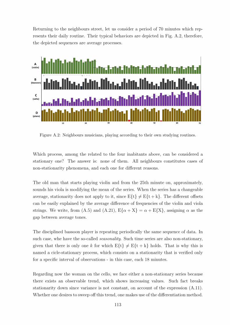
Returning to the neighbours street, let us consider a period of 70 minutes which rep-
resents their daily routine. Their typical behaviors are depicted in Fig. A.2, therefore,
the depicted sequences are average processes.
Figure A.2: Neighbours musicians, playing according to their own studying routines.
Which process, among the related to the four inabitants above, can be considered a
stationary one? The answer is: none of them. All neighbours constitutes cases of
non-stationarity phenomena, and each one for different reasons.
The old man that starts playing violin and from the 25th minute on, approximately,
sounds his viola is modifying the mean of the series. When the series has a changeable
average, stationarity does not apply to it, since Et 6= Et + k. The different offsets
can be easily explained by the average difference of frequencies of the violin and viola
strings. We write, from (A.5) and (A.21), Eα + X = α + EX, assigning α as the
gap between average tones.
The disciplined bassoon player is repeating periodically the same sequence of data. In
such case, whe have the so-called seasonality. Such time series are also non-stationary,
given that there is only one k for which Et 6= Et + k holds. That is why this is
named a cicle-stationary process, which consists on a stationarity that is verified only
for a specific interval of observations - in this case, each 18 minutes.
Regarding now the woman on the cello, we face either a non-stationary series because
there exists an observable trend, which shows increasing values. Such fact breaks
stationarity down since variance is not constant, on account of the expression (A.11).
Whether one desires to sweep off this trend, one makes use of the differentiation method.
113

Moreover, the mean appears in constant modification, which disagrees with the concept
of stationarity.
The conductor is the nearest one to Et 6= Et + k, except in what concerns to
the problem of the outliers. They make variance suffer sudden oscillations, since the
standard-deviation is instantaneously modified. Besides, the expected value does not
remain the same all the time. If the conductor avoids discontinuing his study about
the next concert, probably he would produce a stationary series. Despite of this fact,
many time series like this one are treated with no previous outliers removal, and that
brings no significant loss of exactitude with respect to the results.
A.2.2 Example of a Stationary Series
After visiting so many nonstationary examples, let us characterize a positive case of
stationary process. One of the most curious chracteristics of π is its apparent normality.
A normal number is a real number whose decimal numerals are randomly distributed,
i. e., all numerals appear with the same frequency [59]. We do not know yet if π is
actually normal [60], although there is a lot of speculation in this sense.
Such normality seems to be true, and in function of the several observations that are
made about this number, we can build an example of stationary process. Taking the
first 20000 decimal numerals, and computing the PMF of each one of the 10 digits, we
yield the graph in Fig. A.3.
Figure A.3: PMF of the first 20000 decimal numerals of π.
114
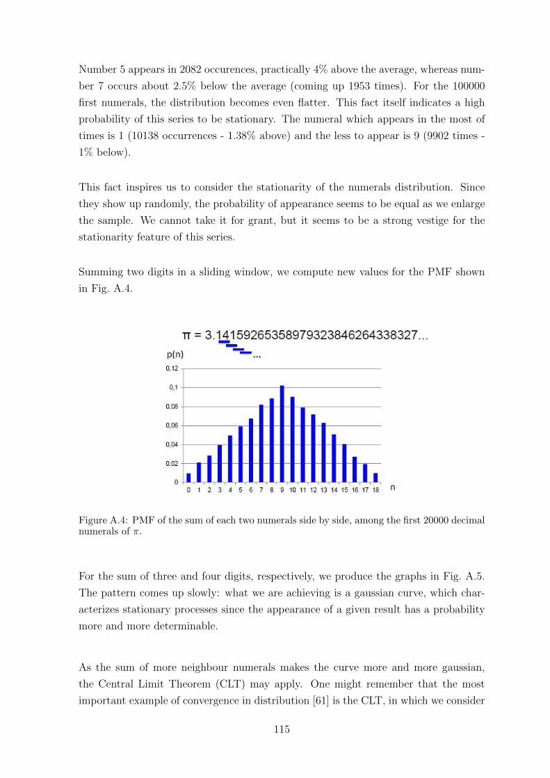
Number 5 appears in 2082 occurences, practically 4% above the average, whereas num-
ber 7 occurs about 2.5% below the average (coming up 1953 times). For the 100000
first numerals, the distribution becomes even flatter. This fact itself indicates a high
probability of this series to be stationary. The numeral which appears in the most of
times is 1 (10138 occurrences - 1.38% above) and the less to appear is 9 (9902 times -
1% below).
This fact inspires us to consider the stationarity of the numerals distribution. Since
they show up randomly, the probability of appearance seems to be equal as we enlarge
the sample. We cannot take it for grant, but it seems to be a strong vestige for the
stationarity feature of this series.
Summing two digits in a sliding window, we compute new values for the PMF shown
in Fig. A.4.
Figure A.4: PMF of the sum of each two numerals side by side, among the first 20000 decimalnumerals of π.
For the sum of three and four digits, respectively, we produce the graphs in Fig. A.5.
The pattern comes up slowly: what we are achieving is a gaussian curve, which char-
acterizes stationary processes since the appearance of a given result has a probability
more and more determinable.
As the sum of more neighbour numerals makes the curve more and more gaussian,
the Central Limit Theorem (CLT) may apply. One might remember that the most
important example of convergence in distribution [61] is the CLT, in which we consider
115

Figure A.5: PMFs of the sum of each three numerals (a) and four numerals (b) side by side,among the first 20000 decimal numerals of π.
random variables to be independent and identically distributed (iid). However, iid
processes are strictly stationary processes. Numerals beyond the comma of π are,
therefore, a probable example of stationary series.
A.2.3 Ergodicity
According to [62], the term ergodic results from the concatenation of two Greek words:
ergos, which means work, and odos = way. This term was introduced in Physics by
the physicist L. Boltzmann.
L. Boltzmann, J. C. Maxwell and J. C. Gibbs were interested in systems which are
described by means of a Hamiltonian flow. Boltzmann believed that the typical flow
orbits filled all the energy surface that contains such flows. Counting on these ergodic
hypothesis, he deduced the the temporal averages of observable measurements along
the typical orbits coincide with the respective spatial means in the energy surface, a
crucial fact for his kinetic theory formulation.
This hypothesis is clearly false; however, in the long run, it became a habit to call as
ergodic hypothesis what should be its consequence, that is to say, spatial and temporal
means being equal.
From [58] we can draw a good explanation of what is an ergodic phenomenon. If Xt is
a variable in a time series, or more generally in a stochastic process, the expectation
is a function of time, µX(t) = EXt. But if the process is stationary, strictly or
116
weakly, µX(t) is a constant, i.e., all variables have the same expectation. Therefore,
a natural question is: can one replace repeated observations of Xt at a fixed t, with
observations of the entire time series, and estimate the common expectation µ by the
time average µn = 1n
∑nt=1 xt, observed in one single realization of the process? The
vector [x1, . . . , xn] is here one observation of [X1, . . . , Xn].
We know, from the law of large numbers, that the average of repeated measurements
converges to the ensemble average µ as n→∞. But would be it equally true for time
average? Does it also converge to µ?
The answer is yes, for some processes. These processes are called ergodic, or, more
precisely, linearly ergodic. A linearly ergodic stationary sequence is a stationary process
Xn, n = 1, 2, . . . where the common mean value µ, which is the ensemble average,
can be consistently estimated by the time average
x1 + x2 + . . .+ xnn
→ µ, (A.44)
where x1, x2, . . . , xn are observations in one single realization of Xt. [58]
The main underlying idea of an ergodic phenomenon is that everything that can happen
in repeated experiments, also happens already in one single realization, if it is extended
indefinitely. Let us remeber the example of the cars plaques given in the beginning
of this Appendix. That team of 50 drivers are again with their cars throughout the
city, each one of them will registering a different sequence of results. Say we select a
random moment to collect the 50 observations. The mean of this of this set of values
is suposed to rest nearby 4.5, since
4.5 =0 + 1 + 2 + 3 + 4 + 5 + 6 + 7 + 8 + 9
10. (A.45)
It is possible that this result stand not very close to 4.5; however, given that it is an
ergodic process, if we enlarge the set of driver from 50 to 5000, the result will approach
4.5 with a considerable certainty. The ergodicity of this phenomenon relies on the fact
that 4.5 is also the result we would get if we analyzed the outcomes from a single
driver, along with several repetitions. The ensemble mean is equal to the mean in
time; whenever it holds, the process is ergodic.
117

Appendix B Z-Transform Models
Modelling is the principle by which one can interact with a real process without facing it
directly. Since the real observed processes and phenomena - mainly in nature and also
considering human relations - are intrinsically nonlinear, models are developed in order
to simplify information to be processed in an indirect perspective. For instance, one
can cite Albert Einstein’s Relativity Theory as a model that allows us to understand
how do mass, space and time behave into specific conditions, truly inaccessible by
any means but imagination. It is very hard to suppose how could anyone reproduce,
without a hugely advanced technology and in a concrete way, the knowledge arisen
from this little set of suppositions; nevertheless, such theory makes possible to build
further theoretic knowledge. Without living or experimenting something by our own
hands, we can still craft a group of ideas and principles that interprete realistic events,
which enables us to understand and control the world that surrounds us.
The underlying idea all over this work, when we cite modelling, is stochastic analysis.
Our capability of forecasting or systematizing apparently indeterminate events is the
core activity into stochastic processes. Consider the ability of determining the increase
in Gross Domestic Product (GDP) in the two next years. A plenty of data which are
still to come up in the real world affect the GDP, nonetheless, the very majority of
the forecasted future GDP lies in the confidence interval. For this reason, they are
a sactisfying model, although they count on data that are seemingly apart from the
reality.
Periodic data forecasts are very related to the Fourier and Laplace transforms, and the
main difference between them is the attenuation term σ. Fourier transform employs
only the frequency of the phasor e−jωt as parameter of integration, being bare of the
this attenuation term. A signal x(t), sampled over periods of length T , has as its
Fourier transform the following complex functions series [63]:
G(jω) = x0 + x1e−jωT + x2e
−jω2T + x3e−jω3T + . . .
118
As said, Laplace transform introduces a little modification consisting on the real part
of the exponent of e:
L(s) = x0 + x1e−sT + x2e
−s2T + x3e−s3T + . . .
The e−sT shift operator provides a T delay between samples, expressed by
e−sT = z−1 = e−(σ−jω)T = e−σT e−jωT = re−jθ, (B.1)
therefore, z = esT is the operator of unitary advance T .
B.1 Background: Z-transform
B.1.1 Definition
Let X be a signal whose values are registered at each period of length T . X is treated as
a discrete process; even if X is a continuous signal, it is sampled in order to be possible
to manage it discretely. The z-transform of a function f(x), which is expressed by
means of its instantaneous values x(n), is given by
F (z) =∞∑
n=−∞xnz
−n. (B.2)
The z-transform of a sampled signal is a series of z−n terms. The zn coefficients are the
temporal sampled values [xn]. Each sample is positioned in the sequence taking into
account the T number of delays, which are provided by the correspondent zn operator,
where the reference is time-origin [63].
The term z, the central piece of this model, is a complex variable. Its two main
properties in this transformation are length and phase.
We can see that Laplace transform is more likely to offer a good paralell to z-transform,
due to the existence of an attenuation factor σ, within s = σ + jω. It is possible to
establish a direct relationship between s and z. In fact, all points from s-plane have a
correspondent point into z-plane. Let s = α+ jβ. The corresponding s-plane point in
z-plane is
119
z = esT
z = e(α+jβ)T = eαT + ejβT ,
therefore,
|z| = eαT
and
angle z = βT.(B.3)
B.1.2 Region of Convergence (ROC)
The result of (B.2) must be summable, i. e., the infinite sum has to converge to a
determined value. When that occurs, X(z) is said to be uniformly convergent. For any
given time series x(n), the set of values of z for which X(z) achieves such convergence
is referred to as the Region of Convergence (ROC).
In (B.3), if we set α = 0, we obtain, in the s-plane, the points belonging to the vertical
axis. If the poles of the Laplace transform of any function lie upon this axis, we have
a critically stabilized function; whether poles are in the α < 0 semi-plane, the function
is stable. Otherwise, the stability is prejudiced. Turning back to α = 0, the equivalent
points into the z-transform are that corresponding to s = jβ, therefore,
|z| = e0 = 1
and
0 < angle z < 360.
When α > 0, then |z| > 1, and, thus, in the z-plane we have the region outside the
unitary circle. Inside this circle, the dual on s-plane is the set of points with α < 0.
The left-side of s-plane corresponds to the interior of the unitary circle of z-plane.
Figure B.1 shows a summarized relationship among the points of the two planes.
This is a mathematical comparison between both planes, which still does not pro-
vide an analysis of convergence; as said, the ROC is the region of z-plane in which
X(z) converges, and such convergence clearly depends on x(n) values. One first glance
over (B.10) would lead us to conclude that, if |z| < 1, the necessary future for X(z)
120

Figure B.1: Relationship among z-plane and s-plane points.
would be infinite values, given the negative exponent of z in Eq. (B.10) and the equiva-
lence established in Fig. B.2. However, |z| < 1 is an isolated information which does not
allow us to conclude X(z) will necessarily diverge. Say, for instance, that x(n) = a−n,
a ∈ R and n = 1, 2, . . ., situation in which X(z) will converge for |z| < |a|:
X(z) =∑∞n=−∞ a
−nz−n
|a−nz−n| < 1
|a−n| < |zn|
|z| > 1a
B.1.3 Behavior of z
The z-transform of the sample signal is a series based on z−1 terms; the coefficients
are the temporal samples xi [63]. Since z is a complex variable, each information
within the time-domain process is assigned to an angle over z-plan, which comes up
in function of the existent T delay-factor α on the e exponent. Therefore, the angular
anti-clockwise displacement, in this plan, is the dual of time running. The length of
z, as above-mentioned, is the parameter related to attenuation. Figure B.2 sketches
three phasor sequences in z-plane, varying the the length of z and its exponent signal.
As said, if z is unitary, only the phase will vary, with no further consequences to the
121

Figure B.2: Behavior of z, depending on |z| and d: (a) |z| < 1, positive exponent (clockwise);(b) |z| > 1, positive exponent; (c) |z| > 1, negative exponent (anti-clockwise).
absolute value of processed signal; this is, by the way, the case in which we have a
Discrete Fourier Transform.
Fig. B.2, (a) shows an decreasing absolute value of z, which makes clockwise displace-
ments. Whether z has a length greater than 1 and d > 0, the spiral will present an
increasing value of its radius, corresponding to (b). If the length of z is less than 1,
but d < 0, then the sequence of z−d results in a spiral whose radius diminishes step by
step, in an anti-clockwise sense (c).
B.1.4 Time-delayed data
The z-transform has great application in sampled signal filtering, with regards to its
capability of delaying data over time. Consider the following system in s-plane, with
a transfer function given by
H(s) = Y (s)X(s)
= 1s,
sY (s) = X(s).
This expression is the same as to say, in time domain, that
dy(t)dt
= x(t).
122

Now, assume that a similar transfer function with the z-transform results in
Y (z) = z−1X(z).
The last expression means that the output y(k) is equal to an input received by the
filter one Ts instant ago, that is, y(k) = x(k − 1). In other words, the observer on the
output side of the filter needs to wait one unit of time to receive the value of input.
The signal x(t) is necessarily associated to the causal part of the system, since y(t) will
receive x(t) information only at the moment t = k + 1. That is the reason why such
z-transform is called as a delay shift operator. Other properties are examined next.
B.1.5 Z-Transform Properties
In [64] there are some interesting properties in of z-transform, and the first one to view,
linearity, turns z-transform into an useful tool for linear signal filters models.
B.1.5.1 Linearity
Zαf1(kT ) + βf2(kT ) = αZf1(kT ) + βZf2(kT ) (B.4)
Proof :
Zαf1(kT ) + βf2(kT ) =∑∞k=0αf1(kT ) + βf2(kT )z−k =
= α∑∞k=0f1(kT )z−k+ β
∑∞k=0f2(kT )z−k =
= αZf1(kT )+ βZf2(kT )
B.1.5.2 Time-Shifting
Zf(k + n) = znF (z)− znn−1∑k=0
f(k)z−k (B.5)
Proof :
Zf(k + n) =∑∞k=0 f(k + n)z−k =
∑∞l=n f(l)zn−l = zn
∑∞l=n f(l)z−l =
= zn∑∞l=0 f(l)z−l −∑n−1l=0 f(l)z−l =
= znF (z)− zn∑n−1k=0 f(k)z−k
123

B.1.5.3 Unitary Advance Operator
Equation (B.30) allows us to consider the compex variable Z as an unitary advance
operator, provided that f(0) = 0. In other words,
zF (z) = Zf(k + 1) (B.6)
This is the dual of the delay shift operator seen before.
B.1.5.4 Initial Value Theorem
If y(kT ) has Y (z) as z-transform and the limit
limz→∞ Y (z),
then there exists
y(0) = limz→∞
Y (z) (B.7)
Proof :
Y (z) =∑∞k=0 y(kT )z−k = y(0) + y(1)z−1 + y(2)z−2 + y(3)z−3 + . . . =
= y(0) + y(1)z
+ y(2)z2 + y(3)
z3 + . . .
Applying limit, we achieve
limz→∞ Y (z) = limz→∞[y(0) + y(1)z
+ y(2)z2 + y(3)
z3 + . . .] = y(0)
B.1.5.5 Final Value Theorem
If F (z) converges for |z| > 1 and if every pole of (z-1)F(z) are into the unitary
circle, then
limk→∞
f(k) = limz→1
(z − 1)F (z) (B.8)
124
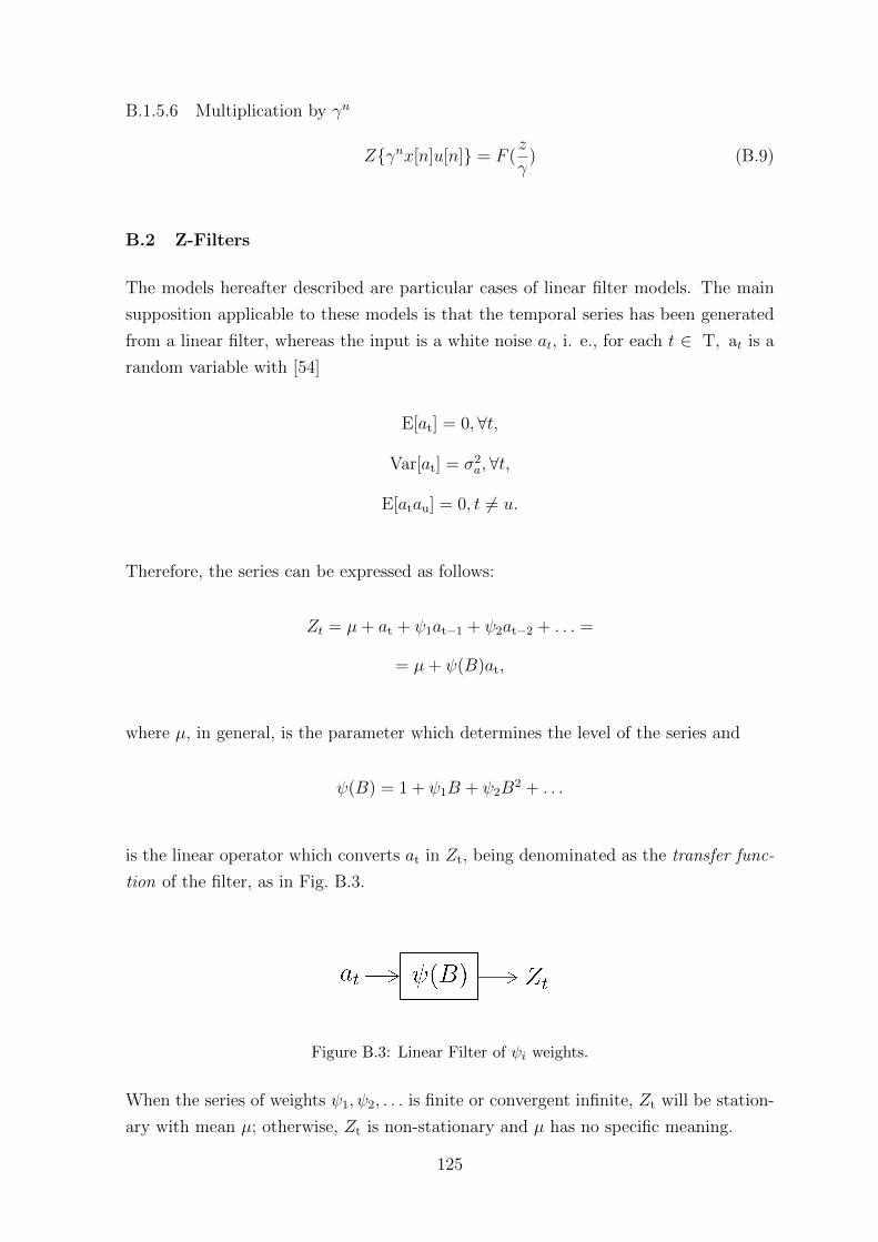
B.1.5.6 Multiplication by γn
Zγnx[n]u[n] = F (z
γ) (B.9)
B.2 Z-Filters
The models hereafter described are particular cases of linear filter models. The main
supposition applicable to these models is that the temporal series has been generated
from a linear filter, whereas the input is a white noise at, i. e., for each t ∈ T, at is a
random variable with [54]
E[at] = 0,∀t,
Var[at] = σ2a,∀t,
E[atau] = 0, t 6= u.
Therefore, the series can be expressed as follows:
Zt = µ+ at + ψ1at−1 + ψ2at−2 + . . . =
= µ+ ψ(B)at,
where µ, in general, is the parameter which determines the level of the series and
ψ(B) = 1 + ψ1B + ψ2B2 + . . .
is the linear operator which converts at in Zt, being denominated as the transfer func-
tion of the filter, as in Fig. B.3.
Figure B.3: Linear Filter of ψi weights.
When the series of weights ψ1, ψ2, . . . is finite or convergent infinite, Zt will be station-
ary with mean µ; otherwise, Zt is non-stationary and µ has no specific meaning.
125

One filter is causal if its impulse response is zero for negative time, φ(n) = 0, for n < 0.
Filters which operate in real time are obviously causal. The time-invariance property
is present when, in face of an excitation v(n− k), the response of the filter is u(n− k),
no matter what is the value of the time shift k. Considering these concepts, a causal
and time-invariant filter is stable if and only if all of the poles of the filter’s transfer
function lie inside the unit circle in the z-plane. This statement, however, says nothing
about the zeros of the transfer function, which can be situated everywhere in z-plane
[65].
The structure of linear filters concerns basically to what is the type of interaction
between input and output data:
• Autoregressive models, or AR, when just the past values of the output variable
are considered as input information;
• Moving Average models, or MA, when the input data is based on white noise
process values - therefore, no past values of the output are taken into account;
• Autoregressive - Moving Average models, the so called ARMA models, which
combines the AR and MA concepts.
There are many possibilities of new models based on other aspects: in the presence of
exogeneous inputs, the process will receive an “X” in its name to indicate “eXogeneous”
or “eXternal” inputs, as in the ARMAX process. In this type of model, more than
one exogeneous data, or auxiliary variables, can be adopted into the process. In the
ARIMA model, we need to eliminate previously the non-stationarity of the input data,
so that the “I” means integration of the values after processing. A large amount of
processes can be generated combining many different characteristics, as in MA, AR,
ARX, etc.
These possibilities may be organized using parameters of a generalized equation. One
can represent [4] a large number of members of AR-MA families by means of this basic
model, corresponding to Fig. B.4, which comprises two inputs, W and U , as well as
their transfer functions, respectively, H(z) and G(z). The output is Y (z). Let the
system be invariant on time and let X be a small perturbation related to stationary
stochastic process.
126

Figure B.4: General System for Stochastic and Deterministic Inputs [65].
The z-transform of the output is
Y (z) = G(z)U(z) +H(z)W (z), (B.10)
where G(z) is the transfer function concerning to the deterministic input U and H(z) is
the transfer function related to the stochastic part of the system W (z). The functions
G(z) and H(z) are stable and rational. H(z) has still these properties:
1. H(z)−1 is stable;
2. limz→∞H(z) = 1.
It is admissible to suppose that the stochastic and the deterministic parts have some
poles in common. From that, we can rewrite (B.10) in order to achieve (B.11):
Y (z) =z−dB(z)
F (z)A(z)U(z) +
C(z)
D(z)A(z)W (z), (B.11)
where A(z), B(z), C(z), D(z) and F (z) are polynomials in z. The poles and zeros of z
correspond to the stochastic and deterministic parts of the system, and d is the delay
of system transport. Taking the inverse of the z-transform of (B.11), (B.12) arises.
A(q−1)y(k) = q−dB(q−1)
F (q−1)u(k) +
C(q−1)
D(q−1)w(k), (B.12)
127

Figure B.5: Infinite Impulse Response (IIR) Digital Filter [63].
In (B.12), q−1 is the delay operator so that y(k)q−1 = y(k− 1), w(k) is the white noise
and A(q−1), B(q−1), C(q−1), D(q−1) and F (q−1) are polynomials defined as follows:
A(q−1) = 1 + a1q−1 + . . .+ anaq
−na
B(q−1) = b0 + b1q−1 + . . .+ bnb
q−nb
C(q−1) = 1 + c1q−1 + . . .+ cncq
−nc
D(q−1) = 1 + d1q−1 + . . .+ dnd
q−nd
F (q−1) = 1 + f1q−1 + . . .+ fnf
q−nf (B.13)
Depending on what are the particular values of A(q−1), B(q−1), C(q−1), D(q−1) and
F (q−1), we obtain different models in terms of system identification [65].
B.2.1 Infinite Impulse Response (IIR) and Finite Impulse Response (FIR)
The complex variable z−i delays the signal in i sample intervals. Assuming that the
transfer function contains a and b terms, we can write the resulting function at a k
instant as
y(k) + a1yk−1 + . . .+ anayk−na = b0xk + b1xk−1 + . . .+ bnbxk−nb
.
We illustrate the z-transform system of Fig. B.5, in which we can observe the input xk
and the ouput yk.
128

Figure B.5 depicts an Infinite Impulse Response (IIR) Filter. This name is due to the
existence of output feeding the input signal back, enforcing the output to be a non-zero
value even when the input disappear. If feedback terms are set to zero, an = 0, then
the system constitutes a Finite Impulse Response (FIR) model, whose output values
depend only on the input signal values [63].
The IIR filter exists when at least one nonzero pole remains in the model not being
canceled by any zero. Hence, the impulse response on the filter has an infinite duration,
since a nonzero pole from A(z) provides output to regenerate input signals indefinitely.
A FIR filter is sometimes described as another particular type of another IIR filter.
The convolution sum of the system impulse response h(k) and the input signal x(n) is
given by
y(k) =∞∑j=0
h(j)x(k − j) + w(k), (B.14)
where w(k) is a white noise actuating over the system. Equation (B.14) is also called
as Infinite Impulse Response (IIR), but the cause of the “infinite response” here is the
infinite sum which involves infinite input terms. If the system is stable, there is an
M <∞ such that h(k) < ε,∀k > M . Hence, we can truncate equation (B.14) in order
to obtain the finite impulse response (FIR), which is given by
y(k) =M∑j=0
h(j)u(k − j) + w(k), (B.15)
where M is the number of elements of impulse response. The FIR model can be
obtained from Eq. (B.12) by making A(q−1) = C(q−1) = D(q−1) = F (q−1) = 1. Here,
B(q−1) consists in an arbitrary polynomial of order M , that is to say, nb = M , in
conformity with Eq. (B.13). In this particular case, FIR model can be written as
y(k) = q−dB(q−1)u(k) + w(k), (B.16)
since, in (B.16), there is an implicit sum until the nb− th term. Nevertheless this filter
is sometimes named as FIR in the bibliography, its underlying principle depends on a
non-truncated input signal, therefore consisting rather in an “Infinite Input Signal”.
129
The infinite impulse is actually obtained, as said, by means of the output to feed the
input filter back, with at least one nonzero pole which is not canceled by any zero.
The forecasted output, y(k|k − 1, θ), corresponds to
y(k|k − 1, θ) = q−dB(q−1)u(k). (B.17)
The output predictor may be represented in the regression form, with the regression
vector, ϕ(k), and the parameters vector, θ, defined as in
ϕ(k) = [u(k − d) . . . u(k − d− nb)]T
θ = [b0 . . . bnb]T
and
y(k|k − 1, θ) = ϕ(k)T θ. (B.18)
Given a situation in which only the deterministic inputs are considered, a dynamic
system cannot be described sufficiently just by means of a FIR model. However, if
system is stable and its impulse response decays rapidly, normally a dynamic system
can approximately place a FIR model, and the model’s precision will rely on the order
of polynomial B(q−1).
B.2.2 Forecasted Error Model (FEM)
An important parameter that helps us to predict future values of output signal is the
“Forecasted Error Model” (FEM), given the fact that output values are, in general,
unpredictable given its stochastic characteristic. Therefore, it is important to know in
the current instant, (k − 1), which is the most probable output in the next instant k
in order to allow the error reduction. That is the reason we estimate the parameters
vector of the process at each instant, so that the predicted error ε is reduced as possible.
The equation of FEM is given by [66]
ε(k, θ) = y(k)− y(k|yk−1, uk−1, θ), (B.19)
130

where y(k|yk−1, uk−1, θ) is the predicted next output value, y(k), as a function of the
model vector parameters θ and of the set of the observed values until instant (k−1) of y
and u, i. e., yk−1 = [y(k−1), y(k−2), . . . , y(0)] and uk−1 = [u(k−1), u(k−2), . . . , u(0)].
One can notice that yk−1 and uk−1 store values since the beginning of the process, which
might represent an additional exigency in terms of computational memory.
Applying the inverse of z-transform to (B.10),
y(k) = G(q−1; θ)u(k) +H(q−1; θ)w(k) (B.20)
In (B.11), we have recognized the existence of the z−d term in the numerator with U ,
the predictable series of input values, meaning that there is, at least, one delay instant
between output and predictable input. In other words, in the first instant of the whole
process, the output does not “see” the values coming from the input related to the
predictable series, which only happens from the d − th instant on. Therefore, we can
write G(0, θ) = 0. If we make G(q−1; θ) = q−1G1(q−1; θ), it follows that
y(k) = q−1G1(q−1; θ)u(k) +H(q−1; θ)w(k),
y(k) = [1-H−1(q−1; θ)]y(k) + q−1H−1(q−1; θ)G1(q−1; θ)u(k) + w(k).
Defining P (q−1; θ) = q[1 − H−1(q−1; θ)] and Q(q−1; θ) = H−1(q−1; θ)G1(q−1; θ), we
achieve
y(k) = P (q−1; θ)y(k − 1) +Q(q−1; θ)u(k − 1) + w(k).
We can obtain from (B.21), explicitly, the forecasted next output of the system for a
particular value of the estimator vector θ = θ:
y(k|yk−1, uk−1, θ) = P (q−1; θ)y(k − 1) +Q(q−1; θ)u(k − 1) (B.21)
For each model hereafter exploited, the FEM method is used to provide us the general
structure of the predictor vector θ. In the analyzed linear systems, at each step y is
compared with the real y and, given that the observations y(k) and u(k) are available
all process long, θ is the equalization factor between predicted value and the real one.
Thus, θ is the vector of coefficients which appear along Eq. (B.13) lines.
131

B.2.3 AR(X) and MA Models
B.2.3.1 Auto-Regressive Model (AR)
The AR structure is obtained by rewriting (B.13) making B(q−1) = C(q−1) = D(q−1) =
F (q−1) = 1, being A(q−1) a polynomial, such that
A(q−1)y(k) = w(k). (B.22)
In time domain, (B.22) can be written in the form
(1 + a1q−1 + a2q
−2 + . . .+ anaq−na)y(k) = w(k). (B.23)
The AR structure, as well as the ARX and ARMAX, considers the last na values of
y(k), including the present value. Therefore, this set of values is made as to comprise
data into a moving-time window. As E[w(k)] = 0, the weights aniare supposed to
convert the average value of A(z)Y (z) into zero within the time-domain.
B.2.3.2 Moving Average Model (MA)
The MA model comes up when we make A(q−1) = B(q−1) = D(q−1) = F (q−1) = 1,
being C(q−1) any polynomial with order nc. The white noise signal have successive
values processed over the filter weights. The output in each instant is supposed to
approach the instantaneous y(k) value:
yk = C(q−1)wk,
yk = (1 + c1q−1 + . . .+ cnq
−n)wk.(B.24)
If wk = 0, we have E[yk] = 0. It means that, in the k-instant, if the white noise is zero
instaneously, y(k) is expected to be zero, that is to say, if n moments of wk = 0, the
average value of the several yk values must approach zero as n increases.
132

B.2.3.3 Auto-Regressive Model with eXogeneous Inputs (ARX)
The ARX structure is obtained by rewriting Eq. (B.13) in order to make C(q−1) =
D(q−1) = F (q−1) = 1, being A(q−1) and B(q−1) arbitrary polynomials, resulting in
A(q−1)y(k) = q−dB(q−1)u(k) + w(k). (B.25)
Since the noise signal w(k) appears explicitly in (eq08), ARX model belongs to the
class of models which present an error term in the equation. As well as FIR model,
ARX can be written in the form
y(k) =q−dB(q−1)
A(q−1)u(k) +
1
A(q−1)w(k). (B.26)
In this case, the noise which is added to the output, e(k) = w(k)A(q−1)
, is not white; in this
model, the white noise w(k) is filtered along an auto-regressive model.
An alternative way of representing ARX model structure correspond to establishG(q−1; θ)
and H(q−1; θ) as
G(q−1, θ) = q−dB(q−1)
A(q−1)H(q−1, θ) =
1
A(q−1), (B.27)
in which the predictor can be written in the form
y(k|k − 1, θ) = q−dB(q−1)u(k) + [1− A(q−1)]y(k) =
= ϕT (k)θ (B.28)
with
ϕ(k) = [y(k − 1) . . . y(k − na), u(k − d) . . . u(k − d− nb)]T (B.29)
θ = [−a1 . . . − ana , b0 . . . bnb]T
(B.30)
From (B.30), one can notice that there is only an algebric relation between the fore-
casted output and the data comprising past inputs and measured outputs.
133

B.2.3.4 Auto-Regressive Moving Average with eXogeneous Inputs (ARMAX)
ARMAX models are produced when, in (B.13), D(q−1) = F (q−1) = 1 and A(q−1),
B(q−1) and C(q−1) are arbitrary polynomials, resulting in
A(q−1)y(k) = q−dB(q−1)u(k) + C(q−1)w(k). (B.31)
Like ARX model, ARMAX is said to bear “error in equation”. Once more, the non-
white noise (perturbation) is modeled as the output of an ARMA filter, in which the
input is the white noise. In face of the A, B, C, D, E and F values, the polynomials
G and H are chosen as below:
G(q−1, θ) = q−dB(q−1)
A(q−1)H(q−1, θ) =
C(q−1)
A(q−1), (B.32)
from where we obtain the predictor:
y(k|k − 1, θ) = q−d B(q−1)C(q−1)
u(k) +(1− A(q−1)
C(q−1)
)y(k)
y(k|k − 1, θ) = q−dB(q−1)u(k) + (C(q−1)− A(q−1))y(k)− (1− C(q−1))y(k|k − 1, θ)
y(k|k − 1, θ) = q−dB(q−1)u(k) + [1− A(q−1)]y(k) + [C(q−1)− 1]ε(k, θ)
= ϕT (k, θ)θ, (B.33)
where ε(k, θ) = y(k) − y(k|k − 1, θ) corresponds to the forecast error or residue. The
regression vector and the parameter vector are defined, respectively, as
ϕ(k, θ) = [y(k − 1) . . . y(k − na), u(k − d) . . . u(k − d− nb), ε(k, θ) . . . ε(k − nc, θ)]T ,(B.34)
and
θ = [−a1 . . . − ana , b0 . . . bnb, c1, . . . cnc ]
T (B.35)
In this case, the predictor model is specified by the roots of polynomial C(z), which
must be inside the unitary circle on the z-plan to assure that the predictor is stable.
Moreover, the presence of the poles in this predictor model causes the regression vector
to depend on the model parameters, meaning that there exists a non-linearity in the
predictor equation (B.33) with regards to θ.
134

Appendix C Examples of Peak Load Reductions over the
Substations in Leipzig Map
In this Appendix, figures depict several examples of reductions for peak load on Leipzig
districts.
In these simulations, we consider that the three emergent sources start to generate from
the 1st week of 2002, therefore w = 156. Only parameters c and a vary. Predictions
are based on ARMAX filter, whose parameters are [10 10 10 1]. As in the Chapter
5, there is a table into each figure containing the parameters c and a for each source,
as well as the year whose last week is forecasted and the color code exposed on the
Fig. 5.13 is inserted.
We should remember that c is the initial amount of generators for each source, such
that it expresses units for antennas and eels, and m2 for PV panels. For the sake of
simplicity, all Power Substations present the same c and a related to the sources in
each figure.
Figure C.1: Peak load reduction by district for the last week of 2006, c = 500 and a = 0.6,antennas only.
135

Figure C.2: Peak load reduction by district for the last week of 2006, c = 1500 and a = 1.0,antennas only.
Figure C.3: Peak load reduction by district for the last week of 2006, c = 1500 and a = 1.0for antennas, c = 200 and a = 1.0 for eels.
136
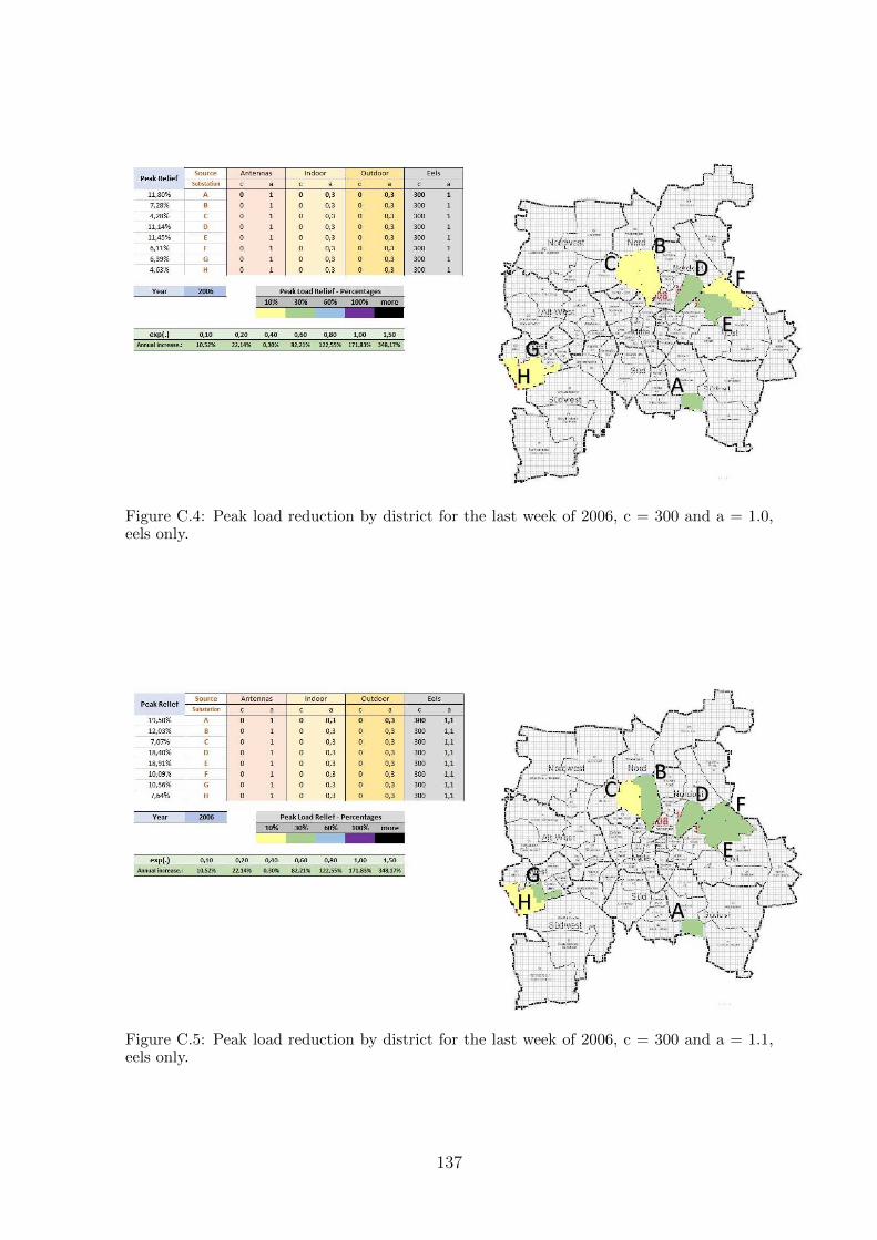
Figure C.4: Peak load reduction by district for the last week of 2006, c = 300 and a = 1.0,eels only.
Figure C.5: Peak load reduction by district for the last week of 2006, c = 300 and a = 1.1,eels only.
137

Figure C.6: Peak load reduction by district for the last week of 2006, c = 300 and a = 1.2,eels only.
Figure C.7: Peak load reduction by district for the last week of 2006, c = 50 and a = 0.6,indoor panels only.
138

Figure C.8: Peak load reduction by district for the last week of 2006, c = 50 and a = 0.7,indoor panels only.
Figure C.9: Peak load reduction by district for the last week of 2006, c = 50 and a = 0.8,indoor panels only.
139
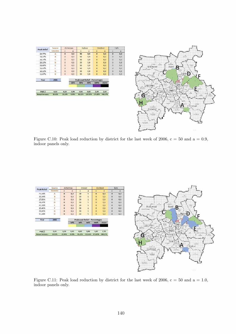
Figure C.10: Peak load reduction by district for the last week of 2006, c = 50 and a = 0.9,indoor panels only.
Figure C.11: Peak load reduction by district for the last week of 2006, c = 50 and a = 1.0,indoor panels only.
140
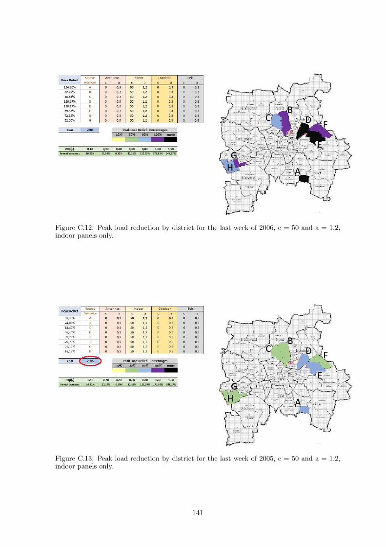
Figure C.12: Peak load reduction by district for the last week of 2006, c = 50 and a = 1.2,indoor panels only.
Figure C.13: Peak load reduction by district for the last week of 2005, c = 50 and a = 1.2,indoor panels only.
141
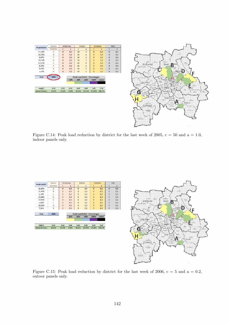
Figure C.14: Peak load reduction by district for the last week of 2005, c = 50 and a = 1.0,indoor panels only.
Figure C.15: Peak load reduction by district for the last week of 2006, c = 5 and a = 0.2,outoor panels only.
142

Figure C.16: Peak load reduction by district for the last week of 2006, c = 5 and a = 0.3,outoor panels only.
Figure C.17: Peak load reduction by district for the last week of 2006, c = 5 and a = 0.4,outoor panels only.
143

Figure C.18: Peak load reduction by district for the last week of 2006, c = 10 and a = 0.4,outoor panels only.
Figure C.19: Peak load reduction by district for the last week of 2006, c = 15 and a = 0.4,outoor panels only.
144
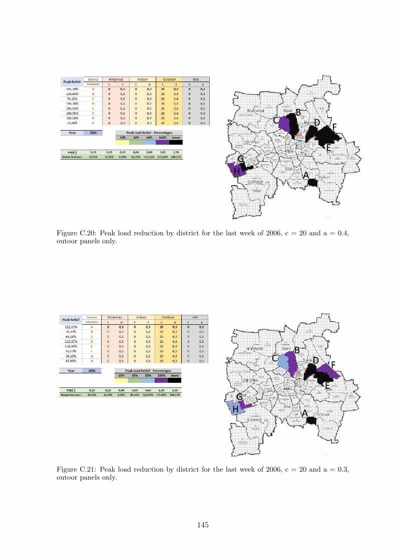
Figure C.20: Peak load reduction by district for the last week of 2006, c = 20 and a = 0.4,outoor panels only.
Figure C.21: Peak load reduction by district for the last week of 2006, c = 20 and a = 0.3,outoor panels only.
145

Figure C.22: Peak load reduction by district for the last week of 2005, c = 20 and a = 0.3,outoor panels only.
Figure C.23: Peak load reduction by district for the last week of 2005, c = 15 and a = 0.3,outoor panels only.
146