CONTRACTOR REPORT SAND97-2426 Unlimited Release

* UC-705

Penetration Equations

C. W. Young Applied Research Associates, Inc. 4300 San Mateo Blvd. NE, Suite A-220 Albuquerque NM 871 10

Prepared by Sandia National Laboratories Albuquerque, New Mexico 87185 and Livermore, California 94550

Sandia is a multiprogram laboratory operated by Sandia Corporation, a Lockheed Martin Company, for the United States Department of Energy under Contract DE-AC04-94AL85000.

Approved for public release; distribution is unlimited.

Printed October 1997

(clir) Sandia National Laboratories

Issued by San&a National Laboratories, operated for the United States Department of Energy by Sandia Corporation. NOTICE This report was prepared as an account of work sponsored by an agency of the United States Government. Neither the United States Govern- ment nor any agency thereof, nor any of their employees, nor any of their contractors, subcontractors, or their employees, makes any warranty, express or implied, or assumes any legal liability or responsibihty for the accuracy, completeness, o r usefulness of any information, apparatus, prod- uct, or process disclosed or represents that its use would not infringe pri- vately owned rights. Reference herein t o any specific commercial product, process, or service by trade name, trademark, manufacturer, or otherwise, does not necessarily constitute or imply its endorsement, recommendation, or favoring by the United States Government, any agency thereof, or any of their contractors; or subcontractors. The views and opinions expressed herein do not necessarily state or reflect those of the United States Govern- ment, any agency thereof, or any of their contractors.

Printed in the United States of America. This report has been reproduced dmectly from the best available copy.

Avadable t o DOE and DOE contractors from Office of Scientific and Technical Information P.O. Box 62 Oak Ridge, TN 37831

Prices available from (615) 576-8401, FTS 626-8401

Avadable to the public from National Technical Information Service U.S. Department of Commerce 5285 Port Royd Rd Springfield, VA4 22161

NTIS price codes Printed copy: A03 Microfiche copy: A01

t

SAND97-2426 Distribution Category UC-705

Unlimited Release Printed October 1997

Penetration Equations

C. W. Young Applied Research Associates, Inc

4300 San Mateo Blvd. NE, Suite A-220 Albuquerque, NM 87 1 10

Sandia Contract No. AN6295

Abstract In 1967, Sandia National Laboratories published empirical equations to predict penetration into natural earth materials and concrete. Since that time there have been several small changes to the basic equations, and several more additions to the overall technique for predicting penetration into soil, rock, concrete, ice, and frozen soil. The most recent update to the equations was published in 1988, and since that time there have been changes in the equations to better match the expanding data base, especially in concrete penetration. This is a standalone report documenting the latest version of the Young/Sandia penetration equations and related analytical techniques to predict penetration into natural earth materials and concrete.

Intentionally Left Blank

.. 11

Contents Section 1 Introduction .................................................................................................................... 1 Section 2 Background .................................................................................................................... 2

2.1 Journal of Soil Mechanics and Foundations, 1969 (5) .......................................................... 2 2.2 Equations for Complex Targets, 1972(6' .............................................................................. 2 2.3 Equations for Penetration of Ice, 1974") .............................................................................. 2 2.4 An Update on the Basic Penetration Equations, 1988'*' ...................................................... 3 2.5 SAMPLL Code (97 lo) ............................................................................................................. 3 2.6 Recent Developments in the Penetration Equations ............................................................ 3

Section 3 Penetration Equations ..................................................................................................... 4 3.1 Penetration Equations for Soil, Rock, and Concrete Targets ............................................... 4

3.3 Nose Performance Coefficient, N ........................................................................................ 6

for Target Materials ........................................................................................................ 8 4.1 S-number for Rock ............................................................................................................... 8 4.2 S-number for Concrete ......................................................................................................... 9 4.3 S-number for Soil ............................................................................................................... 10 4.4 S-number for IceFrozen Soil ............................................................................................. 11 4.5 S-number for Other Materials ............................................................................................ 11

Section 5 Accuracy of the Young Penetration Equations ............................................................ 12 Section 6 Techniques for Calculating Penetration into

Layered Targets ............................................................................................................. 13 6.1 Basic Soil and Rock Layering Technique .......................................................................... 13 6.2 Layering Technique, Concrete Structures .......................................................................... 14

Section 7 Scaling Laws ................................................................................................................ 17 7.1 Geometric Scaling Laws .................................................................................................... 17 7.2 Modifications to Geometric Scaling .................................................................................. 18

Section 8 Conclusion .................................................................................................................... 20 References ..................................................................................................................................... 2 1 APPENDIX A Penetration Equations in SI Units ...................................................................... A- 1 APPENDIX B Penetration Equations Summarized ................................................................... B-1 Distribution ................................................................................................................................... 22

. 3.2 Penetration Equations for Ice and Frozen Soil ..................................................................... 5

Section 4 Methods for Selecting or Calculating S-Numbers

Table 4.1 . Descriptive Terms for Rock Quality. Q ........................................................................ 9 Table 4-2 . Penetrability (S-number) of Typical Soils .................................................................. 11

Table 7-2 . Concrete Target Related Terms .................................................................................. 18 Table 7- 1 . Penetrator Related Terms ............................................................................................ 17

Table 7-3 . Other Target Related Terms ........................................................................................ 18 Table 7-4 . Scaling of Kinematics/Loading/Stress Terms ............................................................. 18

I

... ll1

Summary As part of the Earth Penetrating Weapon (EPW) program at Sandia National Laboratories (SNL), empirical equations are used to predict the depth of penetration into concrete and natural earth materials, and to estimate the average and peak axial deceleration. Equations for soil and rock penetration were published in 1967,11972 and 1988, and these basic equations have changed little over the past 30 years. New equations have been developed for other materials, such as ice, concrete and frozen soil. Theire have been new targets to consider, such as weathered rocks, which have raised questions regarding which equation is correct for certain applications. Finally, new experimental data have led to limited changes in the basic equations. These changes, new equations, new database, and inew’taqgets for the EPW have caused difficulty in the engineering application of the empirical equations;. Perhaps of greater importance is the fact that the primary use of the equations today is as subroutines in computer codes to predict overall penetration performance or weapon effectiveness. The purpose of this report is to clarify some of the resulting questions and to give guidelines to aid in estimating target penetrability.

iv

Nomenclature This report is written in U. S. units, but the nomenclature section and all equations are repeated in Appendix A using SI units.

a A d dn D g K Ke

Ks K3 L Ln ( In N P Q S SK SR tc T fc’ V v e x W W/A CRH 0

Kh

Average acceleration, units of gravity Cross sectional area, psi Penetrator diameter, inches Depth at which nth layer begins, ft Penetration distance, ft Unit of gravity, 32.2 ft/s2 Geometric Scale Factor Correction for edge effects in concrete target A correction factor for lightweight penetrators, hard targets A correction factor for lightweight penetrators, soft targets Factor to account for soil abovehelow concrete layer Penetrator length, inches Length of penetrator nose, inches Subscript refers to the nth layer of a layered target Nose performance coefficient, dimensionless Percent reinforcement, by volume, percent Rock quality, O.l<Q < 1 .O Penetrability of target, S-number, dimensionless Weighted average S-number Reference S-number Cure time of concrete, years (tc 5 1) Target layer thickness, ft Unconfined compressive strength, psi Impact velocity, f p s Exit velocity, f p s Weight of penetrator, Ibs Weight to Area ratio, psi Caliber Radius Head, tangent ogive nose shapes Impact Angle, relative to target surface, degrees

V

Section 1 Introduction

Sandia fiist began its earth penetration program (which was later named “terradynamics”) in 1960, with the objective of developing the technology to permit the design of a nuclear earth penetrating weapon (EPW). The combination of greatly enhanced groundshock due to coupling, and reduced radioactive fallout made a nuclear EPW very attractive. By the mid 1960’s the feasibility of such a weapon had been demonstrated, and a significant experimental data base had been developed.

The combination of a broad data base using full scale penetrators, and the capability of instrumenting the penetrators to measure deceleration during penetration resulted in a sound basis for developing an analytical capability. The basic empirical penetration equations, as published in 1967“’, were based on an extensive experimental data base. These equations have undergone only slight modifications, but the expanding data base and new applications of the equations have required occasional updates. The latest modifications of the equations and the associated analytical technique for predicting penetration by kinetic energy projectiles are summarized in this report.

For those readers who have used the YounglSandia penetration equations for many years, the changes are detailed in the following section, along with the reasons for those changes.

1

Section 2 Background

Before Sandia began its terradynamics program, the problem of penetration mechanics had been studied both analytically and experimentally for over 300 years. During World War II, the Germans developed and tested a penetrator called the Roeschling Round, and the Allied Forces developed and tested several versions of a very large Semi-Armor Piercing (SAP) weapon. However, the technology of penetration mechanics was in its infancy. The most commonly used predictive equations were the Petry elquations (2), based on the earlier Poncelet equation^'^). The penetration equations developed and published in 1967 were referred to as the “Sandia” earth penetration equations. Recently Dr. Michael Forrestal, SNL, also developed and published penetration equation^^^). To differentiate between the two different Sandia equations, the equations presented in this report are referred to as the Young equations, if necessary for clarification, or simply the penetration equations.

Following the publication of the basic penetration equations, the following sequence of publications document the changes o:r additions to the equations:

2.1 Journal of Soil Mechanics and Foundations, 1969 (5)

Prior to the 1967 publication of the penetration equations(’), the Sandia terradynamics program was classified, and there were few foirmal publications on the subject. In 1969, the basic penetration equations were published in the Journal of Soil Mechanics and Foundations(’).

2.2 Equations for Complex Targets, 1 972(6)

In the two earlier publications, a crude method of calculating penetration of layered targets was presented. As more data became available it was possible to refine that technique. A modification of the technique allowed calculation of penetration using complex penetrator shapes, such as penetrators with terrabrakes or detachable afterbodies. The 1972 report covers both layered targets and complex penetrators, but the basic penetration equations were not changed.

2.3 Equations for Penetration of Ice, 1974”)

During the early 1970’s, Sandia conducted a number of ice penetration tests into both sea ice and freshwater ice. It was found that the lbasic penetration equations did not adequately fit the ice data, and a new equation was developed and published. The ice penetration equation was similar to the soilhockkoncrete equation, but the mass (weight) term was different.

2

2.4 An Update on the Basic Penetration Equations, 1988(8)

In about 1979, a new equation was developed to better fit the rock and concrete data. This equation was identical to the earlier equation except the exponent for the Weight-to-Area ratio (W/A) term was 1 .O, instead of 0.5 as used in the basic equations, and the constant was changed to normalize the equations so the penetrability numbers were consistent. The new equation did in fact fit the concrete data better. The new equation also fit the rock data, but the fit was limited to the existing data and not correct in general.

The new and old equations were identical at a W/A of 16 psi. The only available rock data was at W/A ratios close to 16 psi, so the data fit both equations equally well. It was incorrectly assumed that rock penetration would be more similar to concrete penetration than soil penetration, so the new equation was used for both rock and concrete penetration. Even though an extensive data base on rock penetration existed, it was not until about 1983, when the data base was extended to lower W/A ratios, that the new equation (W/A to the first power) was found to not adequately fit the rock data. After 1983, the original equation (W/A to the .5 power) was used for rock and soil penetration, and the more recent equation (W/A to the first power) was used for concrete penetration.

These reversals in recommended penetration equations for rock and concrete were obviously confusing to the user community, and a new report to clarify the issue was published. In addition, an equation to calculate the penetrability of concrete (as opposed to estimating the value) had been developed and was first published in the 1988 report.

2.5 SAMPLL Code (9,101

All of the above reports include only penetration equations. However, the penetration equations and all of the other related analytical techniques are incorporated into the Simplified Analpcal Model of Penetration with Lateral Loading ( S A M P L L ) code. The SAMPLL code goes beyond axial penetration and includes lateral loading and the resulting kinematics, and even penetrator damage or failure. This report, however, includes only penetration equations.

2.6 Recent Developments in the Penetration Equations

In the 1988 report (*), it was recognized that penetration data in frozen soil matched the ice penetration equations. Recently, it was recognized that the ice/frozen soil equation was not consistent with the soil/rock/concrete equation. The new equation for ice/fiozen soil corrects that inconsistency.

It was also recently determined that at very high W/A ratios the concrete penetration equation did not match the new data being obtained. This lack of data fit was not significant at moderate W/A ratios, which included @e vast majority of the experimental data. Based on a new review of all experimental data it was determined that the by using a W/A exponent of 0.7 a single equation would adequately fit the data from all soil, rock and concrete tests. The same equation is now used for soil, rock and concrete.

3

Section 3 Penetration Equations

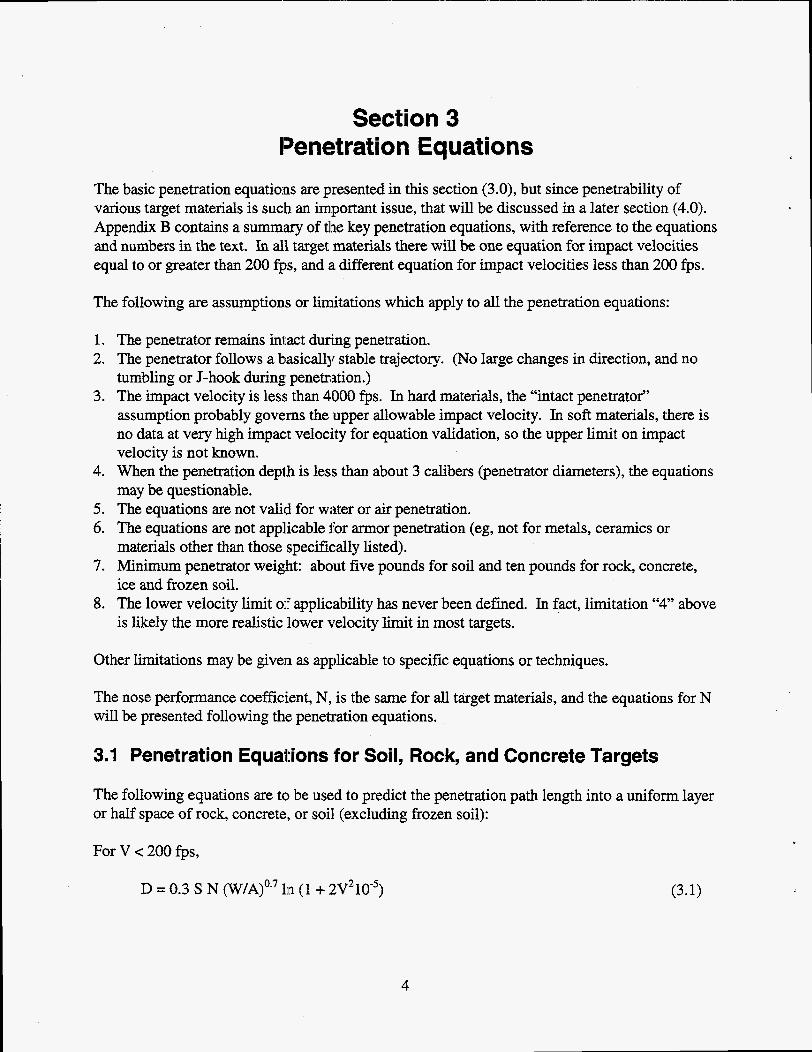
The basic penetration equations are presented in this section (3.0), but since penetrability of various target materials is such an important issue, that will be discussed in a later section (4.0). Appendix B contains a summary of tlhe key penetration equations, with reference to the equations and numbers in the text. In all target materials there will be one equation for impact velocities equal to or greater than 200 f p s , and ii different equation for impact velocities less than 200 fps.

The following are assumptions or limitations which apply to all the penetration equations:

1. 2.

3.

4.

5. 6.

7.

8.

The penetrator remains intact during penetration. The penetrator follows a basically stable trajectory. (No large changes in direction, and no tumbling or J-hook during penetration.) The impact velocity is less than 4000 f p s . In hard materials, the “intact penetrator” assumption probably governs the upper allowable impact velocity. In soft materials, there is no data at very high impact velocity for equation validation, so the upper limit on impact velocity is not known. When the penetration depth is less than about 3 calibers (penetrator diameters), the equations may be questionable. The equations are not valid for water or air penetration. The equations are not applicable for armor penetration (eg, not for metals, ceramics or materials other than those specifically listed). Minimum penetrator weight: about five pounds for soil and ten pounds for rock, concrete, ice and frozen soil. The lower velocity limit of applicability has never been defmed. In fact, limitation “4” above is likely the more realistic lower velocity limit in most targets.

Other limitations may be given as applicable to specific equations or techniques.

The nose performance coefficient, N, is the same for all target materials, and the equations for N will be presented following the Penetration equations.

3.1 Penetration Equaltions for Soil, Rock, and Concrete Targets

The following equations are tcl be used to predict the penetration path length into a uniform layer or half space of rock, concrete, or soil (excluding frozen soil):

For V c 200 fps,

D = 0.3 S N (W/A)0.7 ln (1 + 2:V210-’)

4

For V 2 200 f p s ,

D = 0.00178 S N (W/A)'" (V - 100) (3.2)

In those cases where the penetrator has a tapered body, the cross sectional area, A, is calculated using the average body diameter. The same is true when a flare is used, but only during the portion of penetration when the flare is in contact with the target.

Equations 3.1 and 3.2 have to be modified when the penetrator weight is low, and only in this respect is there a difference between the soil penetration equations and the rockkoncrete equations. When the weight is lower than the limits given below, the right side of Equations 3.1 and 3.2 has to be multiplied by the appropriate term IC

For soil (soft target material):

K~ = 0.2(w)O.~, else, Ks = 1.0

when W c 60 lbs

For rock and concrete (hard target materials):

Kh = 0.4 (W)'.'', else, Kh = 1.0.

when W < 400 Ibs

(3.3)

(3.4)

Often the penetrators weighing less than either 60 pounds (soil) or 400 pounds (rocWconcrete) were scale model penetrators, and therefore the "K" term (Equations 3.3 or 3.4) was referred to as a weight or mass scaling term. Perhaps it is a matter of semantics, but it is recommended that the above K terms be used to account for lightweight penetrators. Any reference to scaling should be limited to scaling laws as discussed in a later section of this report.

3.2 Penetration Equations for Ice and Frozen Soil

The following equations are to be used for penetration into ice (freshwater or sea) and frozen saturated soil:

For V c 200 f p s ,

D = 0.04 S N (W/A)OS6 In (1 + 2V210-5) In (50 + .OW2) (3.5)

For V 2 200 fps,

D = .OW234 S N (W/A)o.6 (V - 100) In (50 + .06W2) (3.6)

Equations 3.5 and 3.6 are known to be applicable in all ice, and in fully frozen soil when the soil is at least 80% saturated. In dry and unfrozen soil, Equations 3.1 and 3.2 apply, but there is

5

insufficient data to define the transition between the frozen soil equations and the unfrozen soil equations. In most applications, the worst case scenario of hard frozen soil is appropriate. For the analysis of penetration data where the material may be either partially frozen or dry, the user will have to judge whether the material is more nearly characterized as being frozen or unfrozen.

In the 1974 ice penetration report” and the 1988 general penetration equation report(8), the ice/frozen soil equations were published with the constants exactly double the values shown here in Equations 3.5 and 3.6 (0.04 and 0.000234, respectively). However, the S-numbers for ice and frozen soil were exactly one half the currently recommended values. The problem is that an inconsistency arose over pene:trabiliqy being defined by how hard a material is to penetrate.

As an example of the relation between S-number and penetrability, a moderately soft concrete (S = 1.0) is five times as hard to penetraite as hard soil (S = 5.0). Likewise, the deceleration during penetration of the concrete would be five times as high as the soil penetration. However, using the earlier equations, ice would have an S-number of 2.0. The implication was that ice was only twice as easy to penetrate as concrete:. The fact is that ice is approximately four times easier to penetrate than concrete. The new S-number for ice and frozen soil, as presented in a later section of this report, used in Equations 3.5 and 3.6, will result in the correct penetration depth and average deceleration level. The user is cautioned not to use the previously published S-number in the new equations. The old S-number used in the old equations” and 8, will give exactly the same answer as the new S-number (tlhis report) in the new equations (this report). One advantage of the new system is that the new S-number, as an indicator of resistance to penetration, is consistent with the S-number of all other materials. A second advantage of the new system is that the transition from frozen to unfi-ozen soil is more “intuitively” correct.

3.3 Nose Performance Coefficient, N

All of the above penetration equations include a Nose Performance Coefficient, N. Originally N was developed based on soil penetration data, and most of the data was from tests at relatively low impact velocity. It was later proven that the same coefficient applies when the target materials are rock, concrete, ice and frozen soil, and M e r that there appears to be no velocity dependence. The following equations can be used to calculate the nose performance coefficient for tangent ogive and conic nose shapes:

For tangent ogive nose shapes, either of the following two equations may be used:

N = 0.18 LJd + .56

N = 0.18 (CRH - .25)0.5 + .56

For conic nose shapes:

N = 0.25 L.Jd + .56.

6

(3.7)

(3.8)

(3.9)

Unfortunately, there are many nose shapes that are neither ogive nor conic, so the following guidelines are recommended:

1.

2.

Approximate true nose shape with an ogive or conic shape: For example, a Mk 84 nose is not an ogive, even when it has the pointed tip (that is, no nose fuze). A 6 CRH ogive approximates the M k 84 nose shape reasonably well, and the error will not be more than about 5%. Blunted nose shapes: If the blunting (either a flat or a 90 degree included angle conic tip) is less than 10% of the penetrator diameter, it can be ignored. If the blunted tip is larger, Equation 3.7 should be modified as:

N = .09 (L + L')/d + .56 (3.10)

where L' is the actual nose length, after the original (not blunted) length is reduced by the blunting, and similarly Equation 3.9 becomes:

N = .125 (L,, + L')/d + .56 (3.1 1)

A nose performance coefficient, also referred to as N, is used in both the F~rrestal'~) and NDRC"" penetration equations. The general effect of the nose shape on penetration is similar among all the equations, but the magnitude of N itself is different.

7

Section 4 Methods For Selecting Or Calculating S-Numbers

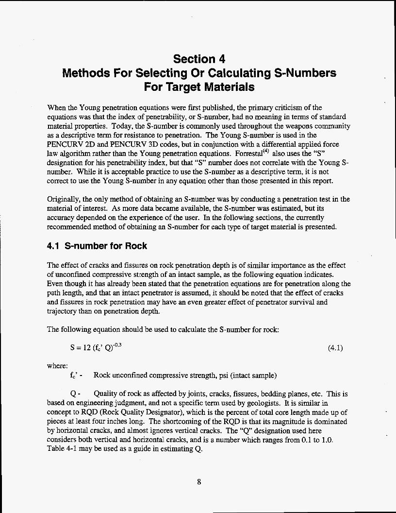
For. Target Materials When the Young penetration equations were first published, the primary criticism of the equations was that the index of penetrability, or S-number, had no meaning in terms of standard material properties. Today, the S-number is commonly used throughout the weapons community as a descriptive term for resistance to penetration. The Young S-number is used in the PENCURV 2D and PENCURV 3D codes, but in conjunction with a differential applied force law algorithm rather than the Young penetration equations. Forresd4) also uses the “S” designation for his penetrability index, but that “S” number does not correlate with the Young S - number. While it is acceptable practice to use the S-number as a descriptive term, it is not correct to use the Young S-number in any equation other than those presented in this report.

Originally, the only method of obtairung an S-number was by conducting a penetration test in the material of interest. As more data be:came available, the S-number was estimated, but its accuracy depended on the experience: of the user. In the following sections, the currently recommended method of obtaining an S-number for each type of target material is presented.

4.1 S-number for Rock

The effect of cracks and fissures on rock penetration depth is of similar importance as the effect of unconfined compressive strength of an intact sample, as the following equation indicates. Even though it has already been stated that the penetration equations are for penetration along the path length, and that an intact penetrator is assumed, it should be noted that the effect of cracks and fissures in rock penetration may .have an even greater effect of penetrator survival and trajectory than on penetration depth.

The following equation should be used to calculate the S-number for rock

S = 12 (fc’ Q)-0‘3

where: fc’ - Rock unconfined compressive strength, psi (intact sample)

(4.1)

Q - Quality of rock as affected by joints, cracks, fissures, bedding planes, etc. This is based on engineering judgment, and not a specific term used by geologists. It is similar in concept to RQD (Rock Quality Designator), which is the percent of total core length made up of pieces at least four inches long. The shortcoming of the RQD is that its magnitude is dominated by horizontal cracks, and almost ignores vertical cracks. The “Q’ designation used here considers both vertical and horizontall cracks, and is a number which ranges from 0.1 to 1 .O. Table 4-1 may be used as a guide in estimating Q.

8

Table 4-1. Descriptive Terms for Rock Quality, Q

DescriDtive Terms Q

Massive Interbedded Joint Spacing e 0Sm Joint Spacing > 0.5m Fractured, blocky, or fissured Highly fractured or jointed Slightly weathered Moderately weathered Highly weathered Frost shattered Rock Quality, very goodexcellent Rock Quality, good Rock Quality, fair Rock Quality, poor Rock Quality, very poor

0.9 0.6 0.3 0.7 0.4 0.2 0.7 0.4 0.2 0.2 0.9 0.7 0.5 0.3 0.1

A considerable amount of judgment is required in selecting a value for Q. Jf two or more of the above terms are used, it will be necessary to condense the aggregate descriptions into a single value of Q. If the type and extent of weathering is already accounted for in the Unconfined compressive strength, then there is no need to include it again in Q. And fmally, terms like “joint spacing” and “fractured” will have a different Q depending on the size of the spacing relative to the penetrator diameter. Unfortunately, there is insufficient data to be more explicit. Other analytical techniques typically use a reduced unconfined compressive strength to account for cracks and fissures, which has the same effect as Q in Equation 4.1, but is even more difficult to quantify.

If the S-number, as calculated using Equation 4.1, is above 3.5, the material is probably better defined as being a hard soil. If the S-number is between 2.5 and 3.5, even the geologists may disagree as to whether it is soil or rock. There are no strict recommendations for this range of materials, but the following guideline may be useful. If the unconfined compressive strength of an intact sample can physically be measured by normal means, Equation 4.1 probably applies.

4.2 S-number for Concrete

The following equation should be used to calculate the S-number of concrete.

S = 0.085 K, (1 1 - P) (&T,)-0.06 (5000/fc’)0~3 where:

9

P - This is the volumetric: percent rebar, which is not the percentage as normally used in civil engineering practice. Since rebar in the direction perpendicular to the surface of the target also affects penetrability, “P” is given on the volumetric basis. Most concrete targets have from 1% to 2% rebar.

- Cure time, years, Jf t, > 1, then set & = 1. This cure time is independent of the effect of cure time on unconfined coinpressive strength.

T, - Thickness of target, in penetrator diameters or calibers. If the target is made up of multiple thinner layers, each layer must be considered individually. When T, < 0.5, this equation may be inadequate because thle mechanisms of penetration are different. If T, > 6, use T, = 6.

f,’ - Unconfined compressive strength at test time (not 28 day strength), psi. (It may be necessary to estimate the strength at test time, based on 28-day strength.)

& = (F/w*)0.3 (4.3)

Where, W1= Target width, in. penewator calibers. If W1> F, then & = 1. F = 20 for reinforced concrete, and 30 for no reinforcement. For thin targets (thickness 0.5 to 2 calibers), the values for F should be reduced by 50%.

In those cases where insufficient data exits to pennit calculating the S-number for concrete, a default value of S = 0.9 is reciommended.

The estimated accuracy of Equation 4.2 is lo%, which is approximately the same as typical data scatter. This statement is true. “most” of the time, but no “sigma” value should be associated with this estimate. There is limited validation of Equation 4.2 for very high strength concrete (> 18OOO psi), and low strength concrete (-1000 psi).

4.3 S-number for Soil

The data base for soil penetration is far more extensive than for other materials, and yet estimating an S-number for soil is more difficult than for other materials. Table 4.2 gives some examples which will help guide the user in selecting a suitable S-number. In addition to the table, the following guidelines should be considered:

1. It is unusual (but not impossilAe) for soil below a depth of about 50 feet to be softer than S = 15. The exceptions are marine-type clay sediments, such as in the Gulf of Mexico or the Great Salt Lake Basin,

2. It is also unusual for soils to be harder than S = 5 unless the material is cemented, such as lenses of cemented sand or hyers of caliche, both of which are normally found in desert environments.

3. The penetrability of clay, and to a lesser degree silt, is very dependent on moisture content.

10

4. The penetrability of sand is almost independent on moisture content. In mixtures of sand/silt/clay, only about 20% to 30% silt or clay is required to make a material behave more like silt or clay (ie, dependent on water content).

5. The ease with which a soil can be excavated by hand (shovel) is not a good guide as to its penetrability. A stiff clay is very hard to dig and is easy to penetrate, but a loose sand is easy to dig and hard to penetrate.

Table 4-2. Penetrability (S-number) of Typical Soils

S-number 2 - 4

4 - 6 6 - 9

8 - 10 5 - 10

10 - 20 20 - 30 30 - 60

> 60

Target Descriu tion Dense, dry, cemented sand. Dry caliche. Massive gypsite and selenite deposits. Gravel deposits. Sand, without cementation. Very stiff and dry clay. Moderately dense to loose sand, no cementation, water content not important. Soil fill material, with the S-number range depending on compaction. Silt and clay, low to medium moisture content, stiff. Water content dominates penetrability. Silt and clay, moist to wet. Topsoil, loose to very loose. Very soft, saturated clay. Very low shear strength. Clay marine sediments, either currently (Gulf of Mexico) or recent geologically (mud deposits near Wendover, Utah). It is likely that the penetration equations do not apply.

4.4 S-number for Ice/frozen soil

Both fresh water ice and sea ice will normally have an S-number of 4.5 & 0.25. Completely frozen saturated soil will have an S-number of 2.75 & 0.5. The S-number of partially frozen soil may be as high as 7.0, but the transition from partially frozen to unfrozen soil is not well defined.

4.5 S-number for Other Materials

The penetration equations do not apply to the penetration of water, armor, and air, as discussed in Section 3.0. The applicability of the equations to other materials is unknown, but S-numbers have been determined for the following materials: (Use these S-numbers with caution.) 1. S = 1.5: Multiple sheets of plywood stacked together. (Frequently used to stop a penetrator

after it has perforated the desired target.) 2. S = 2 to 3: Boulder fields, with air between the boulders. 3. S = 2 to 4: Rock rubble. (Rock rubble is defined as the material excavated from a rock

formation.)

11

Section 5 Accuracy Of The Young Penetration

Equations It is virtually impossible to differentiate between the accuracy of the penetration equations and the accuracy of the S-number.. Considering the normal data scatter and the variability of concrete and geologic materials, all coimments on accuracy are estimations; that is, the inaccuracy values given are correct “most” of the time. Multiple penetration tests into similar (but not identical) targets indicated that the penetration equations have an inaccuracy of about 10% from the mean. It can be assumed that the inaccuracy increases somewhat near the end of the range of applicability, but that has not been quantified. When the term for lightweight penetrators is applicable (Kh or Ks), the inaccuracy is likely to be greater.

The equation for the S-numbex of concrete appears to have an inaccuracy of 10%. The combined inaccuracy of the equations (penetration equation and S-number equation) is about 15% to 20%.

The equation for the S-number of rock has an inaccuracy of 20% (when the data is very good) to as much as 100% (when the data, especially the Q-value, is little more than a guess). For rock penetration, the penetration equation inaccuracy can essentially be ignored in comparison to the inaccuracies in the rock description. The variance in the rock description as reported by two or more geologists can easily be as great as the combined errors in the equations.

12

Section 6 Techniques For Calculating Penetration Into

Layered Targets There are several applications of the penetration equation which involve layered targets. The two most common are the penetration of natural soil formations and the penetration of underground structures. The layering equations and techniques presented below are recommended for natural soil targets, but the SAMPLL code is recommended for calculating penetration into underground structures.

6.1 Basic Soil and Rock Layering Technique

The objective of the soil and rock layering technique is to better predict penetration distance. The approach is to calculate the average deceleration and the velocity change during penetration of each layer, until finally a layer cannot be penetrated at the current velocity. The resulting calculated deceleration versus depth curve can be used to approximate the deceleration during penetration, but it will be a very simplified approximation. A rule of thumb is that the peak deceleration in any one layer will be about 1.3 times the calculated average deceleration.

The general technique presented below is the same as published in 1972‘6’, but with the current penetration equations. The majority of geologic formations encountered by penetrators are layered, and using a single S-number for these layered targets will result in significant errors. The following technique is recommended:

Step 1. Calculate SK for each target layer, using Equation 6.1 below.

Step 2: Calculate Sn, using Equation 6.2 below.

Step 3: Calculate Dn, using Equation 3.1 or 3.2, with S , and Vn. Dn is the penetration distance into the nth layer distance, or to calculate the average deceleration in the nth layer, as discussed in steps 4 and 5, respectively.

if the nth layer were infinitely thick. It is used as either part of the total

Step 4: If Dn If Dn > Tn/sin 0, continue to the next step.

Tn/sin 8, then Dto& = d,/sin 8 + Dn, where Dtod is the total penetration distance.

Step 5: Calculate the average acceleration in the nth layer, using Equation 6.3 below.

Step 6: Calculate Vn+l, using Equation 6.4 below. Obviously the exit velocity from the “n” layer is the same as the impact velocity of the “n+l” layer.

Step 7: Repeat Steps 1 through 4 for the next or “n + 1” layer.

13

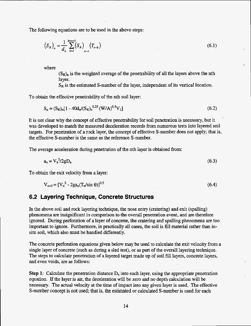
The following equations are to be used in the above steps:

where (SK),, is the weighted average of the penetrability of all the layers above the nth layer. SR is the estimated S-number of the layer, independent of its vertical location.

To obtain the effective penetrability of the nth soil layer:

It is not clear why the concept of effective penetrability for soil penetration is necessary, but it was developed to match the measured deceleration records from numerous tests into layered soil targets. For penetration of a rock layer, the concept of effective S-number does not apply; that is, the effective S-number is the !;ame as the reference S-number.

The average acceleration duriiig penetration of the nth layer is obtained from:

To obtain the exit velocity from a layer:

Vn+1= [ ~ , 2 - 2gan(Tdsin e)l0.:j

6.2 Layering Technique, Concrete Structures

(6.4)

In the above soil and rock layering technique, the nose entry (cratering) and exit (spalling) phenomena are insignificant in comparison to the overall penetration event, and are therefore ignored. During perforation of a layer of concrete, the cratering and spalling phenomena are too important to ignore. Furthermore, in practically all cases, the soil is fill material rather than in- situ soil, which also must be handled differently.

The concrete perforation equations given below may be used to calculate the exit velocity from a single layer of concrete (such as during a sled test), or as part of the overall layering technique. The steps to calculate penetration of a layered target made up of soil fill layers, concrete layers, and even voids, are as follows:

Step 1: Calculate the Penetration disitance Dn into each layer, using the appropriate penetration equation. If the layer is air, the deceleration will be zero and no depth calculation will be necessary. The actual velocity at the time of impact into any given layer is used. The effective S-number concept is not used; that is, the estimated or calculated S-number is used for each

14

layer. Jf the first layer is soil fill material, an S-number of 6 to 10 is used, as given in Table 4.2. If the soil fill is between two layers of concrete, the S-number of the fill is reduced by a factor of two. Similarly, the S-number of the soil below a layer of concrete (such as below the floor of a structure) is reduced by a factor of two, up to a distance of six penetrator calibers.

Step 2: If D, 5 Tn / sin 8, then Dtod = Dnn + Wsin 8. If Dn > Tn/sin 8, continue. For the penetration of underground structures, it may be more convenient to work with vertical depth instead of distance along the penetration path. In that case, D ’ T ~ ~ = dn + Dnsin 9.

Step 3: Calculate an, using Equation 6.3.

Step 4: Calculate Vn+l, using one of the concrete perforation equations given below, or Equation 6.4 above.

Step 5: Repeat Steps 1 and 2 until the final penetration depth (or distance) is determined. During perforation of a layer of concrete, the full level of deceleration does not occur until the nose is fully embedded in the target. This is usually called the “cratering” phase of penetration. As the exit face of a concrete layer is approached, the deceleration begins to reduce, even before the nose tip reaches that surface. This is usually called the “spalling” phase of penetration, even though the term “spall” does not necessarily refer to the tensile failure which OCCUTS due to a reff ected elastic stress wave. When the target is thin, relative to the nose length, the cratering and spalling phases may overlap, requiring a different exit velocity equation.

For the purpose of this discussion, a thick concrete layer is one whose thickness is the greater of one penetrator nose length or one penetrator diameter. The following equation should be used to calculate the exit velocity from a thick concrete layer (the subscripts “n” which refer to the layer being penetrated are omitted for clarity):

Vex = [V2 - 2ga(T/sin 6 - L/K3)]0’5 (6.5)

where,

K3 = (a) 2, for air over and under concrete layer, or (b) 3, for air on one side of the concrete layer, or (c) K, for air on neither side of the concrete layer.

The above values of K3 apply for reinforced concrete. For unreinforced concrete, the values of K3 should be reduced by 0.5.

The following equation should be used to calculate the exit velocity from a thin concrete layer (less than the greater of one nose length or one penetrator caliber):

Vex = [V2 - 2ga(T&sin e)’.* T( 1 - 1/K3)]o.5 (6.6)

The same values of K3 as used above are used in this equation.

15

If the user has no need for the average deceleration in each layer, the following equations may be used to calculate the exit velocity, and Step 3 can be eliminated:

For a layer of fill material: Vex = V[ 1 - T/Dsin

For a layer of thick concrete: Vex = V[ 1 - (Thin 8 - 1L&3)/13]o.5

For a layer of thin concrete:

Vex = V[ 1 - (Ths in 0)O.* (T -. 1/K3)/D]0.5

(6.7)

16

Section 7 Scaling Laws

There are many types of scaling used in various disciplines. A very simple example is “cube root scaling”, as usually applied to blast effect from explosives. Scaling is also used in fluid mechanics, where scaling is accomplished through well established dimensionless terms such as the Reynold’s Number. In penetration mechanics, there have been several unsuccessful attempts to develop similar dimensionless terms for scaling laws.

The most common scaling technique is to use simple geometric scaling, which is described below. The most accurate scaling technique is to use geometric scaling, but modified to better fit experimental data. That is the approach followed in this report, and the penetration equations are used as part of the modification procedure.

7.1 Geometric Scaling Laws

This section covers geometric scaling as normally applied to penetration mechanics. The general approach is to scale the target and penetrator, without changing the density or strength of either, and without scaling the impact velocity. Most other scaled values are the result of the application of this approach. Strain rate is assumed to be negligible. To obtain the desired values for the scale model penetrator, multiply the full scale value by the scale factor, K, to the appropriate power, as shown in tables 7.1 through 7.4.

Table 7-1. Penetrator Related Terms

Diameter

Wall thickness Density of case material Nose shape Case material strength Weight (case or explosives) Area L/d Strain rate effects Center of gravity (distance) Moment of inertia

Length K1 K’ K1 KO KO KO

K2 KO

K’

K3

Assumed none

K5

17

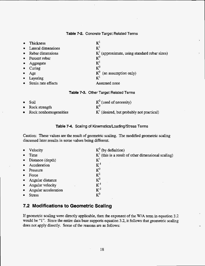
Thickness Lateral dimensions Rebar dimensions Percent rebar Aggregate Curing Age Layering Strain rate effects

Table 7-2. Concrete Target Related Terms

K’ K’

KO K’ KO KO (an assumption only) K’ Assumed none

K’ (approximate, using standard rebar sizes)

Table 743. Other Target Related Terms

Soil Rockstrength Rock nonhomogeneities

KO (used of necessity)

K’ (desired, but probably not practical) KO

Table 7-4. Scaling of Kinematics/Loading/Stress Terms

Caution: These values are the result of geometric scaling. The modified geometric scaling discussed later results in some values being different.

Velocity Time Distance (depth) Acceleration Pressure Force Angular distance Angular velocity Angular acceleration Stress

KO (by definition) K’ (this is a result of other dimensional scaling) K’ K“ KO K2 KO K-l K-2 KO

7.2 Modifications to Geometric Scaling

If geometric scaling were directly applicable, then the exponent of the W/A term in equation 3.2 would be “1”. Since the entire data biise supports equation 3.2, it follows that geometric scaling does not apply directly. Some of the reasons are as follows:

18

1. Curing of concrete targets: While it might be possible to minimize this problem, it may not be worth the effort. However, some rather detailed small scaled testing in the 1930’s demonstrated that curing is a significant problem. For that reason, it is recommended that the extent of scaling be limited to about 113 scale or !A scale.

2. Strain rate effects: This is not generally thought to be a significant problem. 3. Effect of WIA on penetration: This is the major error in geometric scaling. According to

geometric scaling, the penetration depth varies directly with the WIA ratio. According to the Young penetration equations, the depth varies with the WIA to the 0.7 power, and the relation is further modified for lightweight penetrators.

Since the modifications to geometric scaling are based on the penetration equations, it is recommended that scaling be limited to the lower weight limits of applicability of the equations. It is further recommended that the scaling be limited to 1/3 or !A scaling to minimize the errors.

The recommended approach is to use geometric scaling as the baseline. If the objective is to evaluate scale model penetration results, the approach should be to apply the penetration equations to the scale model test results, and then again apply the penetration equations to the full or large scale penetratorharget. That is, geometric scaling is used to scale the target and penetrator, but the penetration equations are used to scale the penetration results (depth, acceleration, stress, force, etc.).

Another application of scaling is to conduct scale model tests to demonstrate or prove a technical objective. If the objective is to evaluate the penetrator structure (stress, deformation, damage, failure, etc.), the approach is to adjust the target strength to give the scaled penetration depth, using the penetration equations to determine the required target modification. If the objective is to evaluate exit velocity from a concrete target, the target thickness can be increased to result in the same exit velocity as the full scale value, again using the penetration equation. In most cases, the error in directly applying geometric scaling is not large, so the modifications to the target or test conditions are not large.

It may appear that if the penetration equations are being used either indirectly or directly as scaling laws, then what is the objective of scale model testing? There is in fact little point in running a small scale penetrator into a small scale target to indirectly determine the penetration performance of a large penetrator. It is more direct to simply use the equations to predict the penetration performance of the large penetrator. However, there are many valid reasons for conducting small scale tests, such as:

1. To compare two or more nose shapes in terms of survivability or relative penetration performance.

2. To optimize the wall thickness of a penetrator configuration. In this case, the target would be modified to result in the appropriate stress in the penetrator case.

3. To determine, at least on a comparative basis, the effect of varying target parameters such as rebar percentage, unconfined compressive strength of concrete, or lateral edge effects.

4. To determine the effect of parameters such as steel ductility or strength on the survivability of a penetrator.

19

Section 8 Conclusions

1. Empirical analytical techniques are presented to predict penetration into rock, soil, concrete, ice, and frozen soil.

2. Techniques and equations are presented to estimate the penetrability of various target materials.

3. The empirical technique for predicting depth into a uniform target material is expanded to include penetration into layered targets.

4. The penetration equations are utilized to improve the basic geometric scaling laws to better understand scale model test data and results.

5. The penetration equations are accurate within approximately 15%, except near the limits of applicability.

6. The penetrability (S-numbler) equation for concrete is accurate within approximately 10%. 7. The accuracy of the equation for the penetrability (S-number) of rock is highly dependent on

the accuracy of the input data, and may vary from 20% to a factor of 2 or more.

20

References 1.

2.

3.

4.

5.

6.

7.

8.

9.

C. W. Young, The Development Of Empirical Equations For Predicting Depth Of An Earth Penetrating Projectile, SC-DR-67-60. Albuquerque NM: Sandia National Laboratories, Albuquerque, NM, May 1967.

L. Petry, Monographies De Systems D 'Artillerie, Brussels, 1910.

Jean V. Poncelet, Cours De Mechanique Zndustrielle, 1829, First Edition.

M. J. Forrestal, B. S. Altman, J. D. Cargile, and S. J. Hanchak, An Empirical Equation For Penetration Depth Of Ogive-Nose Projectiles Into Concrete Targets, Proceedings of the Sixth international Symposium on Znteraction of Nonnuclear Munitions with Structures, pp. 9-32. Panama City Beach, FLY May 3-7, 1993.

C. W. Young, Depth Predictions For Earth Penetrating Projectiles, Journal of Soil Mechanics and Foundations SM3, May 1969.

C. W. Young, Empirical Equations For Predicting penetration PeijCormance In Layered Earth Materials For Complex Penetrator Configurations, SC-DR-72-0523. Sandia National Laboratories, Albuquerque, NM, December 1972.

C. W. Young, Penetration Of Sea Ice By Air-Dropped Projectiles, SLA-74-0022. Sandia National Laboratories, Albuquerque, NM, March 1974.

C. W. Young, Equations For Predicting Earth Penetration By Projectiles: An Update, SAND88-0013. Sandia National Laboratories, Albuquerque, NM, July 1988.

C. W. Young and E. R. Young, Analytical Model Of Penetration With Lateral Loading, SAND84-1635. Sandia National Laboratories, Albuquerque, NM, May 1985.

10. C. W. Young, A Simplified Analytical Model Of Penetration With Lateral Loading (Sampll) - An Update, SAND9 1-2 175. Sandia National Laboratories, Albuquerque, NM, February 1992.

1 1. Joint Services Manual For The Design And Analysis Of Hardened Structures To Conventional Weapons Effect (DAHS CWE Manual), DNA-DAHSCWEMAN-94-CH6 (DRAFT), (publication expected during 1997).

21

APPENDIX A Penetration Equations in SI Units

The Nomenclature section of the full report is repeated below in SI units. All equations requiring SI units are repeated in this appendix. The equation numbers are preceded by an A to differentiate from the equations in the text.

Average acceleration, units of gravity Cross sectional area, m2 Penetrator diameter, m Depth at which nth layer begins, m Penetration distance, m Unit of gravity, 9.8 1 m/s2 Geometric scalle factor Correction for edge effects in concrete target A correction factor for lightweight penetrators, hard targets A correction factor for lightweight penetrators, soil targets Penetrator length, m Penetrator nose length, m Subscript refers to the nth layer of a layered target. Nose performance coefficient Percent rebar in concrete, volumetric percentage Rock quality, 0.1 < 1 .O Penetrability of target, S-number, dimensionless Cure time of concrete, years (& 5 1) Unconfined compressive strength, Mpa Impact velocity, m / s Exit velocity, rds Mass of penetrator, kg Weight (mass) to Area ratio, kg/m2 Caliber Radius Head, tangent ogive nose shape Impact angle, relative to target surface, degrees

A- 1

A-I Penetration Equations for Soil, Rock and Concrete Targets

For V < 61 d s :

D = 0.0008 S N (I~/A)O.~ In (1 + 2.15V2 lo4)

For V 2 61 d s :

D = 0.000018 S N (I~/A)''~ (V - 30.5)

The modifications to the equations for lightweight penetrators are:

For soil (soft target):

Ks = 0.27 (m)'" else, Ks = 1.0.

If m<27kg

(Caution: Equations A-3.1 and A-3.2 may not be applicable when m e 2 kg.)

For rock and concrete (hard targets):

Kh =.46(n~).'~ my 182 kg.

(Caution: Equations A-3.1 and A-3.2 may not be applicable when m e 5 kg.)

A-2 Penetration Equations for Ice and Frozen Soil

For V < 61 d s ,

D = 0.00024 S N (m/A)Oe6 In (1 + 2.15V2 lo4) In (50 + 0.2!h2)

For V 2 61 m/s,

D = 0.0000046 S N (~II/A)O.~ (V - 30.5) In (50 + 0.29m2)

A-3 Nose Performance Coefficients, N

A-3.1

A-3.2

A-3.3

A-3.4

A-3.5

A-3.6

Equations 3.7 through 3.11 are the same in either system of units, and will not be repeated in the Appendix.

A-4 S-number for Rock

S = 2.7 (fc' Q)-0.3 A-4.1

A-2

A-5 S-number for Concrete

S = 0.085 & (1 1 - P) (tc TC)-O.'O6 (35/fc70.3

There is no change to Equation 4.3 for &.

A-6 Basic Soil and Rock Layering Technique

Equation 6.1 for (S& is independent of units.

The SI equation for Sn is:

Sn = (S& [ 1 - 988 d , / ( s~ ) ,O~~ (II~A).~V,]

A-4.2

A-6.2

In equations 6.3 and 6.4, the average ,acceleration during penetration and the exit velocity are not changed.

A-7 Layering Technique, Concrete Structures

Equations 6.5 through 6.9 are not changed.

A-3

APPENDIX B Penetration Equations Summarized

All equations discussed in this report are summarized in this appendix for use as a quick reference. The user should refer to the Nomenclature section for the definition of terms, and to the discussion of each equation in the text for more details of the equation. The equations in this appendix use the same equation numbers as used in the text.

B-I Penetration Equations for Soil, Rock and Concrete Targets

D = 0.3 S N (W/A)0.7 In (1 + 2V210e5), v < 200 fps

D = 0.00178 S N (W/A)0.7 (V - loo), v 2 200 f p s

K~ = 0.2(~)O.~, when W < 60 lbs

when W < 400 lbs

v < 200 f p s

v 2 200 f p s

B-2 Penetration Equations for Ice and Frozen Soil

D = 0.04 S N (W/A)o.6 ln (1 + 2V210-5) In (50 + .Om2),

D = .000234 S N (W/A)o-6 (V - 100) In (50 + .06W2),

B-3 Nose Performance Coefficients, N

Tangent ogives:

Conic shapes:

N = 0.18 L,Jd + .56,

N = 0.25 L/d + .56.

B-4 S-number for Rock

s = 12 (fc' Ql-O.3

B-5 S-number for Concrete

S = 0.085 Ke (1 1 - P) (tcT,)'0.06 (5000/f,')0.3

where:

(3.5)

(3.6)

(3.7)

(3.9)

(4.11

(4.2)

P - This is the volumetric percent rebar, which is not the percentage as normally used in civil engineering practice. Since rebar in the direction perpendicular to the surface of the target

B- 1

also affects penetrability, “P” is givein on the volumetric basis. Most concrete targets have fi-om 1% to 2% rebar.

- Cure time, years. If tc > 1, then set = 1. This cure time is independent of the effect of cure time on unconfined compressive strength.

T, - Thickness of target, in penetrator diameters or calibers. If the target is made up of multiple thinner layers, each layer must be considered individually. When T, < 0.5, this equation may be inadequate because the mechanisms of penetration are different. If Tc > 6, use T, = 6.

f,’ - Unconfined compressive strength at test time (not 28 day strength), psi. (It may be necessary to estimate the strength at test time, based on 28-day strength.)

where

W1 = Target width, in perietrator calibers. If WI > F, then & = 1. F = 20 for reinforced concrete, and 30 for no reinforcement. For thin targets (thickness 0.5 to 2 calibers), the values for F should be reduced by 50%.

B-2

DISTRIBUTION Distribution:

Applied Research Associates, Inc. (10) Attn: Wayne Young (9)

4300 San Mateo Blvd, NE. , Suite A-220 Albuquerque, NM 871 10

Frank Maestas

Applied Research Associates, Inc. New England Division 120-A Waterman Rd. South Royalton, VT 05068

HQDSWA (3) Attn: Dr. Mike Giltrud, SPSD

Dr. Linger, PM Dr. Tremba, PMT

6801 Telegraph Rd. Alexandria, VA 223 10-3398

Field Command, DSWA Attn: FCTT, Dr. Baladi 1680 Texas St. S.E. Kirtland AFB, NM 87 117-5669

US. Army Waterways Experiment Station Attn: Dr. R. Rohani 3909 Halls Ferry Rd. Vicksburg, MS 39180-6199

Wright Lab Armament Directorate (2) Attn: Virgil Miller, MNMW

101 W. Eglin Blvd. Eglin AFB, FL 32542-6810

Scott Teel, MNMF, Ste. 219

Rockwell International Corp. Tactical Systems Division Attn: J.T. Gissendanner 1800 Satellite Blvd. Duluth, GA 30136

22

Texas Instruments, Inc. Attn: Kenneth Stonebraker 151 S. Highway 121 P.O. Box 405, MS 3468 Lewisville, TX 75067

Phillips Laboratory/SXP Attn: Dr. Sandra Slivinski 3550 Aberdeen Ave. S.E. Kidand AFB, NM 871 17-5776

Applied Research Associates, Inc. (2) Shock Physics Division Attn: R.Cilke

P. Roupas P.O. Box 5388 Albuquerque, NM 87 185

Logicon RDA Attn: Mr. Renick P.O. Box 9377 Albuquerque, NM 87 1 19-9377

Springfield Research Facility Am: RickSmith P.O. Box 1220 Springfield, VA 22 15 1-0220

Raytheon Electronic Systems Attn: Donald C. Power MS TlFS13 50 Apple Hill Dr. Tewksbury, MA 01876-0901

Lawrence Livermore National Lab (3) Attn: Technical Library

Larry Altbaum Roger Logan

P.O. Box 808 Livermore, CA 94550

U.S. Geological Survey Attn: Don Percious Reston, VA 22092

Orlando Technology, Inc. Attn: Mike Gunger P.O. Box 877 Shalimar, FL 32579

Northrop G r u m a n Corp. Attn: Ernie Silva, B-2 Division 8900 E. Washington Blvd. Pic0 Rivera, CA 90660-3783

Karagozian & Case Attn: David Bogosian 625 N. Maryland Ave. Glendale, CA 9 1206

Department of the Army U.S. Army Topographic Engineering Cntr. Attn: Karl Koklauner, PD-DT 770 1 Telegraph Rd. Alexandria, VA 22315

Naval Surface Weapons Center Attn: Tim Spivak, Code G-22 Bldg. 221 Dahlgren, VA 22448

SN/AQQS (N) Attn: Lt.Co1. Billy Mullins 1060 Air Force The Pentagon Washington, DC 20330-1060

Tenera Rocky Flats, L.L.C. Attn: Stephen Nicolosi 4949 Pearl East Circle, Ste. 104 Boulder, CO 80301

TASC Attn: Charles Drutman 55 Walkers Brook Dr. Reading, MA 01 867-3297

William J. Patterson 1320 Cuatro Cerro Tr. S.E. Albuquerque, NM 87 123-5607

ANSER, Global Power Division Attn: Bill Bearden 1215 Jefferson Davis Hwy, Ste. 800 Arlington, VA 22202

Hu'ghes Missile Systems Co. (2) Attn: Tom Bootes, Bldg. 805, B-3

Me1 Castillo, Bldg. 805, B-3 Tucson, AZ 85734

University of Arizona Deptartment of Planetary Sciences Attn: Bill Boynton Tucson, AZ 85721

Applied Research Associates, Inc. Southern Division Attn: James Drake 3203 Wisconsin Ave. Vicksburg, MS 39 180

Col. Tom Eastler RFD 1, Mosher Hill Box 1043 Farmington, MA 04938

S A - A L C A " Attn: Ellsworth Rolfs 1651 First St. S.E. Kirtland AFB Albuquerque, NM 871 17-5617

Department of Energy, HQ (2) Attn: Jeff Underwood, DP-22

Glenn Bell, DP-25 Germantown, MD 20874

Department of Energy, AWWPD Attn: MarkBaca P.O. Box 5400 Albuquerque, NM 87185-5400

23

USSTRATCOWJ533 Attn: Stan Gouch 901 SAC Blvd. Ste. 2E9 Offbtt AFB, NE 681 13-6500

HQ ACCLGWN Attn: Michael Hendricks 130 Douglas St. Ste. 210 Langley AFB, VA 23665-2791

Sandia National Laboratory (43) Attn: K.R. EMund, 2102, MS0435

W.R. Reynolds, 2103, MS0427 D. L. McCoy, 2104, MS0453 N. R. Hansen, 2104, MS0453 (10) J.O. Harrison, 21 11, MS0447 W.J. Errickson, 21 11, MS0447 G.L. Maxam, 2147, MS0436 J.R. WifaI1,2147, MS0436 A.B. Cox, 2161, MS0482 S. A. Ken, 2161, MS0482 R. N. Everett, 2263, MS09034 J. P. Hickerson, 241 1, MS0303 T. L. Warren, 24 1 1, MS0303 M.J. Forrestal, 241 1, MS0303 R.G. Lundgren, 241 1, MS0303 J.L. McDowell, 241 1, MS0303 D.E. Ryerson, 2664, MS0987 R. F. Franco, 2664, MSO987 J. D. Rogers, 5412, MS0419 S . W. Hatch, 5413, MS0417 W. H. Ling, 5413, MS0417 S . M. Schafer, 5413, MS0417 H. A. Dockery, 685 1, MS 1326 E.P. Chen, 8742, MS9042 P. Yarrington, 9232, MS0820 S. A. Silling, 9232, MS0820 D.B. Longcope, 9234, MS0439 Central Tech Files, 8940-2, MS9018 Technical Library, 4916, MS0899 (5 ) Review & Approval Desk, 12690,

MS0619 for DOE/OSTI (2)

Los Alarnos National Laboratory (9) Attn: Fred Edeskuty, C936

Richard Macek, P946 Mamy Martinez, P936 John St. Ledger, F607 Mike Schick, F607 Tom Duffey, P946 Mary Roth, P362 Lany Witt, F630 Library

P.O. Box 1663 Los Alamos, NM 87545

24