Performance analysis of distributed implementations of a fractal image compression algorithm

$Page 1: Performance analysis of distributed implementations of a fractal image compression algorithm$
CONCURRENCY PRACTICE AND EXPERIENCE, VOL. 8(5) , 357-380 (JUNE 1996)

Performance analysis of distributed implementations of a fractal image compression algorithm DAVID JEFFJACKSON AND GREG SCOTTTINNEY Department of Electricd Engineering PO Box 870286 The University of Alabama Ti rcnloosa, Alabama 35487, USA

SUMMARY Fractal image compression provides an innovative approach to lossy image encoding, with a potential for very high compression ratios. Because of prohibitive compression times, however, the procedure has proved feasible in only a limited range of commercial applications. In the paper the authors demonstrate that, due to the independent nature of fractal transform encoding of individual image segments, fractal image compression performs well in a coarse-grain distributed processing system. A sequential fractal compression algorithm is optimized and parallelized to execute across distributed workstations and an SP2 parallel processor using the parallel virtual machine (PVM) software. The system utilizes both static and dynamic load allocation to obtain substantial compression time speedup over the original, sequential encoding implementation. Considerations such as workload granularity and compression time versus number of processors and RMS tolerance values are also presented.

1.

In [ I ] , Barnsley introduced a new method of image compression referred to as fractal image compression. With fractal image compression, an image is modeled as a set of fractals and is encoded as such. The term ‘fractal’ was introduced by mathematician Benoit Mandelbrot. By definition, a fractal is ‘a set for which the Hausdorf Besicovitch dimension strictly exceeds the topological dimension’ [2]. A more straightforward description of the phenomenon is a fractured structure possessing similar forms at various sizes 131.

In The Fractal Geometry of Nature [2], Mandelbrot observed that many naturally oc- curring objects also exhibit this self-similarity at smaller scales of detail. For instance, the trunk of a tree in winter has large limbs branching out in all directions, while each of these limbs has smaller limbs (and in turn smaller twigs) that also branch out in a similar manner. With much experimentation, Mandelbrot and others have been able to successfully and compactly model with fractals many natural objects or landscapes, such as clouds, mountains and forests, that are too complex to define with standard Euclidean geometry.

INTRODUCTION TO FRACTAL IMAGE COMPRESSION

1.1. The Sierpinsky triangle

A well-known structure that clearly demonstrates fractal characteristics is the Sierpinsky triangle shown in Figurel.

The triangle is generated by taking an arbitrary image, scaling it by one-half, and translating three copies of the scaled object to form the image shown in Figure 1 (b). If this

CCC 1040-31 08/96/050357-30 @ I 996 by John Wiley & Sons, Ltd.

Received Moy I995

358 DAVID JEFF JACKSON AND GREG SCOTT TINNEY

Figure 1. The Sierpinsky triangle

process is repeated indefinitely, with the output of each step being fed back as the next input, the image of Figure l(e) results. The image in Figure l(e) is known as an attractor. The attractor results because the transformations performed on the image, referred to as affine transformations [4], are contractive. A transformation is described as contractive if and only if all points of a given image are brought closer to each other by the transformation. The contraction mapping theorem [4] states that an infinite sequence of contractive affine transformations on a set will always converge to a single, fixed point. In the case of the Sierpinsky triangle, repeatedly applying several contractive affine transformations on an arbitrary object produces a single, fixed image or attractor. As shown, the Sierpinsky triangle can be produced by the iteration of only three simple transformations on an input image. The transformations labeled wi can be written compactly as the matrix operations

and

w' [ ; ] = [ O: R 5 ] [ ; ] + [ : ]

0.5 0 w [ ;I=[ 0 0 . 5 1 [;I+[ (3)

for a 256 x 256-pixel attractor. The union of contractive transforms, wi, is referred to as an iterated function system (IFS) code [I] . Any given IFS code, consisting of a set of contractive affine transformations, can be used to describe an attractor.

While studying fractals, Barnsley theorized that any given digital image could be treated as an attractor. If the attractor's IFS code could be determined, the contractive affine transformation coefficients could be stored instead of pixel information, resulting in a highly compressed file. The image could then be quickly regenerated by repeatedly applying the IFS transformations to any given input array of pixels.

1.2. The Fractal Transform

Barnsley developed the fractal transform [3] which, though computationally expensive, provides an automated method for determining a unique set of IFS coefficients that define

PERFORMANCE ANALYSIS OF DISTRIBUTED IMPLEMENTATIONS 359

a given digital image. The basis of the fractal transform is the collage theorem. The collage theorem states that the union of contractive affine transformations on an image space define a map (or IFS code) W on the space [5], or

Given an input set (or image) S, a new set or attractor W ( S ) is described by the union (collage) of subimages, each of which is formed by applying a contractive affine transformation w, on S. This theorem is used to define the IFS code for a Sierpinsky triangle as the union of transformations 201,

The collage theorem is also important because it suggests a method of simplifying an image before determining its IFS code. The collage theorem describes an image attractor as the union of one or more subimages, each of which is formed by applying a contractive affine transformation on an arbitrary image. Therefore, when a given digital image is modeled as an attractor, it may be partitioned into subimages (referred to as range blocks), each of which can also be treated as an attractor with its own set of contractive transformations that comprise a local iterated function system or local IFS [4]. The advantage of partitioning an image in this manner is that the smaller range blocks are less complex and can thus be described by a simpler local IFS. The union of these simplified local IFS codes then forms the original image’s partitioned iterated function system or PIFS [5 ] .

As stated, the target subimages are referred to as range blocks. Each range block is an attractor that results when a given set of local IFS transformations is applied repeatedly to an arbitrary subimage of a specific size and location. The union of those range blocks form the original image. The source subimages to which the transformations are applied to form range blocks are referred to as domain blocks. The only restriction on the choice of domain blocks is that each domain block be larger than the range block it models, so that the local IFS transformations that map the domain block to a range block will be contractive. It should be noted that the terms range and domain are reversed in [I], [3], [4] and [6]. For continuity, however, the nomenclature adopted by Fisher [ 5 ] is used.

and w.

1.3. Fractal Image Compression Algorithm

All programs utilized in this research were derived from code by W.D. Young. Young’s fractal compression and decompression programs were based on algorithms presented by Fisher [5] that implemented the forward and inverse fractal transform. A flow diagram for the compression program is shown in Figure2. For compression, the image is partitioned into 1024 non-overlapping, 8 x 8-pixel regions which serve as range blocks, as displayed in Figure 3 . Figure 4 demonstrates how the image is also partitioned into 58,081 overlapping, 16 x 16-pixel domain blocks. By overlapping domain blocks in this manner, all possible 16 x 16 regions of the input image are represented by a corresponding domain block. Thus, all subimages of the proper size may be compared with a given range block to determine an acceptable match. Each range and domain block is categorized as a shade, edge or midrange block by its characteristics, using a classification suggested in [6]. Regions are classified so that a given range block will be compared only with domain blocks that are predetermined to posses similar characteristics, saving many unnecessary comparisons.

Before the images are compared, a method of mapping a domain block onto a range block must be introduced. Previously, a two-dimensional affine transformation was described by


min-distance YES - - <

distance -

BEGIN (2 I Classify Range and Domain Blocks I

& Output min-distance affine map

Figure 2. Sequential fractal image compression algorithm


the matrix operation wi, in the form

w l [ ; ] = [ :: 2 ] [ g ] + [ ; ] where the coefficients ai, b,, ci, and di determined scale, rotation and skew, and e, and fi determined translation. Equation ( 5 ) would prove appropriate for a binary (two-color) image. For a 256-gray scale image, however, domain pixel intensities must also be transformed to match those of a given range block. This can be accomplished by representing the image in three-dimensional space, where the z-axis corresponds to pixel intensity. Incorpo- rating intensity information as a spatial dimension must be performed carefully, however, to ensure that x-y spatial data are not mapped to intensity data, and vice versa, during a three-dimensional transformation. This can be accomplished by the matrix transformation PI

where si controls the contrast and 0, the brightness of vi. Note that s, is multiplied only to z , and 0% is added only to z, so that spatial and pixel intensity information remain independent. This separation of dimensions can be represented compactly by [4]

where wi is the two-dimensional transformation of equation (5) . Using the affine transformation in (6), a domain block’s geometry and pixel intensities can

be mapped to those of a range block for comparison. To compare the similarities between a given range block and a transformed domain block, we must choose a metric which describes the ‘distance’ between the two subimages. One such distance, represented by the variable meansq, between a (one-half) scaled domain block, possessing pixel intensities DI , . . . , Dn, and a range block possessing pixel intensities R1, . . . , R, and dimension n x n, is defined as [5]

n

mean-sq = x[(s. Dj t 0) - RJI2 j = l

Note that the variables s and o must be determined before the distance meansq can be found. Since it is desirable to minimize the distance, we may solve for s and o by taking partial derivatives of meansq with respect to the two variables and setting the results equal to zero. Doing so produces the relations

and


n n

C Rj - s C j = l j = I

0 = n2

To avoid redundant computations, c,”=, R3 is calculated once as each new range block is extracted, while C,”=, D3 and c,”=, 0: are calculated for each domain block during the pre-processing stage and stored in the Domainsurns array. A mean square distance can then be determined by the more computationally efficient form of (8):

.” (11)

Once a range block has been extracted and all orientations have been determined, the first domain block of the same classification is extracted for comparison. Using the mcthod above, the distance between each orientation of the present range block and the extracted domain block (scaled by one-half) is computed. If one of the comparisons results in a mean square distance less than the mean square tolerance specified by the user, a match results. Information describing the local IFS transformations that successfully mapped the domain block to the given range orientation is then stored as the range’s ‘affine map.’ This process of extracting domain blocks with the same classification as the given range block is repeated until a match within the specified tolerance is found. If no match is found, the domain block that most closely matched any of the given range block’s orientations is used and its corresponding affine map is stored.

Once all range blocks have been matched with a similar domain block, the PIFS information is written compactly to a fractal image file. This file consists of an array of structures that stores the following PIFS variables for each range block:

0 dx: the x-offset of the domain block that maps to the present range block 0 dy: the 3-offset of the mapping domain block 0 scale: contrast, or s , transformation coefficient that maps pixel intensities of the

0 ofset: brightness, or 0, pixel intensity mapping transformation coefficient 0 pip: the orientation (rotation) of the range block that incurred a match, and 0 size: the size of the matching domain block before transformation (needed for

domain block at (dx,dy) to those of the present range block

quadtree partitioning).

1.4. Quadtree partitioning

The simple partition method illustrated in Figures 3 and 4 is image independcnt and, therefore, generally does not produce optimal compression ratios. The common geometry and size of range and domain blocks, however, simplifies PIFS encoding and decoding. This characteristic also reduces the storage requirements of each range block’s corresponding affine map, as the range’s location may be easily calculated by the decompression program.

A limitation of this partitioning scheme, however, is the use of a fixed range size. Many regions of a given image are too complex to be partitioned into 8 x 8-pixel squares, because


8

T

\

Range Range Range Block Block Block ""I 0

0 L

0

Range Block

> > Figure 3. Range block partitioning

the image may not possess corresponding 16 x 16-pixel domain blocks that closely match the regions. To overcome this limitation, the compression algorithms for this research use a slightly more elaborate bi-level quadtree partition scheme that increases the fidelity of the regenerated image. During compression, if an 8 x 8 range block cannot be matched to a 16 x 16 domain block within the mean square tolerance, the range block is divided into 4 x 4-pixel range sub-blocks. Each of these sub-blocks are then compared to quadtree partitioned, 8 x 8 domain blocks. When a match is made, the dimension of the range and domain blocks is stored in the one-bit affine map variable size. Range/domain size is designated as either LARGE (8 x 8 range/l6 x 16 domain) or SMALL (4 x 4 range/8 x 8 domain). This size variable is used later during decompression to determine local IFS transformations for domain mapping.

Quadtree partitioning often provides higher compression ratios than the simpler method of Figure 3, because it is more image dependent. In simple regions, LARGE range blocks (requiring one, 40-bit affine map per block) can be used to encode the image compactly. In more complex regions, groups of four SMALL range blocks (requiring four, 40-bit affine maps per group) can be used to encode the image while retaining fidelity. This compression ratio/fidelity trade-off is necessary where the quality of the regenerated images must be high, but where the compression ratio is also important.

In addition to higher compression ratios, quadtree partitioning generally increases the time required to compress an image. Increased compression time results because the algorithm used in this research initially assumes that a given image region can be encoded with

364 DAVID JEFF JACKSON AND GREG SCO" TINNEY

Domain Block

2

\

Domain Block 58080

Figure 4. Domain block partitioning

a LARGE range block. Therefore, a very complex region is first unsuccessfully compared with every 16 x 16 (LARGE) domain block of the same classification before the region is decomposed into four SMALL range blocks. As each range-domain comparison is computationally expensive, these unnecessary comparisons produce a significant impact on the fractal image compression time.

1.5.

To test the performance of the compression and decompression algorithms, the portable greyscale map (PGM) images displayed in Figure 5 were used as input. The first image, boy.pgm, represents a good test case for compression. The boy's relatively featureless and symmetrical face, the large, constant background, and the flat lighting all combine to form an image rich in affine redundancy that can be encoded primarily using LARGE range blocks. By using few SMALL range blocks, the compression algorithm is able to compress boy.pgm relatively quickly and compactly, while retaining adequate fidelity. The image of Lena, however, possesses a more complex background and more intricate detail, requiring a larger proportion of SMALL range blocks to encode than does the first image. This image complexity results in significantly lower compression ratios and longer compression times.

Table 1 displays the compression ratios and execution times, for given RMS tolerances, of the original sequential program designed by Young, and the compression ratios of the sequential code optimized for this research. Execution times for the optimized sequential code are given in Section 2.

Fractal image compression and decompression results


Figure 5. PGM test images

~

I e n a. p g m

Compression ratios at all thresholds are higher for the optimized code than for Young’s code. This is due to changes in the local IFS structure format that reduce PIFS information storage requirements from 48 bits per range block affine map to the 40-bit per affine map level. As seen in Table 1, compression time at all RMS thresholds is considerable. While most lossless methods require only a few seconds to compress images such as thosc of Figure 5, Young’s implementation often requires 15 to 40 minutes to compress the same image with reasonable retention of fidelity. Such long compression times prove prohibitive in mosl applications.

For fractal image compression to be feasible, these execution times must be reduced significantly, and the algorithm’s compression ratios should be increased. A more advanced

Table I . Compression time and ratio versus RMS threshold ~~ ~~

Young implementation Optimized code

RMS Image threshold compression Execution Compression

ratio time,s ratio

10.0 8.5: 1 210 10.2: 1 boY.Pgm 6.0 7.4: 1 348 8.9: 1

3.0 5.2:1 873 6.2: 1

10.0 6.1:l 759 7.3:l 1ena.pgm 6.0 4.7: 1 1337 5.7: 1

3.0 3.5: 1 2403 4.3: 1


partitioning scheme that utilizes feature extraction techniques to encode the image with larger range regions could potentially address the algorithm's relatively low compression ratios. Unfortunately, fractal image compression is a computationally expensive process that does not lend itself well to fast sequential implementation.

It should be noted, however, that the encoding of a given range block of an image is independent of all other range block encodings. Thus, in a parallel system, groups of range-domain comparisons may be distributed across multiple processors and performed simultaneously.

2. SEQUENTIAL OPTIMIZATIONS

As each range block matching is independent of other range block matchings for fractal image compression, the algorithm lends itself readily to parallelization. However, even if a separate processor encodes each range block, locating an appropriately transformed domain block that closely resembles the range block remains a computationally expensive process (especially at low user-defined RMS tolerances). To minimize the time required to perform such a matching, the sequential code provided by Fisher was first optimized to provide efficient sequential execution before parallelization was attempted. As the original code represented an attempt at testing the method outlined in Fisher [5 ] and speed was not a goal of the project, ample opportunities for sequential optimizations were present. In addition to removing unused variables and altering variable names for clarity and consistency, many optimization techniques were utilized to enhance the compression algorithm's sequential operation including: unnecessary code removal, loop concatenation, variable type redeclaration, code motion, strength reduction and common subexpression elimination. Additionally, code was rewritten, from gcc compliance, to be compatible with the more advanced IBM xfc compiler. Although details of these optimizations are not important to this research, results of the performed optimizations are shown in Figure 6.

These results display the performance augmentations that can be achieved by optimizing a given program. The results also reveal the considerable disparity between the optimization capabilities of different compilers currently in use. As much of the high-level optimizations are standard among modern C compilers, these disparities are probably contingent on a given compiler's utilization of architecture-specific optimizations such as efficient pipeline utilization and integer-floating point instruction parallelization. With the efficient code a faster parallel compression algorithm can be derived, as much of the computationally intensive operations in the distributed system must be executed in a straight-line(sequentia1) manner on individual processors.

3. DISTRIBUTED WORKSTATION PARALLEL SYSTEM IMPLEMENTATION

The image compression algorithm discussed belongs to the coarse-grain parallel class of processes implemented using a master/slave computational model. The bulk of the program consists of range block matchings, each of which require alarge number of complex floating point computations that are independent of any other such comparisons. Apart from the distribution of work and initial data among nodes and the return of results to a common node, little inter-processor communication is required. Thus, the parallel implementation consists of powerful node processors, with advanced floating point capabilities, while communication efficiency is here considered secondary.


Sequential Fractal Compression Time vs. RMS original and optimized code using 2 mmpilers (boy image)

2500'0 t L

2000.0 A H optimized-gcc

0.0 ' 2.0 3.0 4.0 5.0 6.0 7.0 8.0 9.0 10.0

user-defined RMS

Sequential Fractal Compression Time vs. RMS original and optimized code using 2 compilers (/en8 image)

)--1 optimized-gcc 2500.0

1000.0 -

500.0

0.0 ' 2.0 3.0 4.0 5.0 6.0 7.0 8.0 9.0 10.0

user-defined RMS

Figure 6. Optimized sequential execution times


In this case, the parallel system consists of up to 16 IBM RW6000 workstations interconnected in a token ring network. Inter-node communication is managed by parallel virtual machine (PVM). PVM is a software system that permits a network of heterogeneous UNIX computers to be used as a single large parallel machine (referred to as a virtual machine) [71.

3.1. Parallel Load Balancing

The purpose of parallelizing any algorithm is to augment the application’s performance by decreasing its execution time. For maximum speedup, however, the effects of standard parallel limitations such as inter-process dependency and inter-node communications should be minimized. Another innate problem of distributed processing is load balancing. Load balancing, the method in which work is disbursed among processors (in this case, particular range block matchings to individual slave nodes), is often the most critical aspect of parallel implementation. If the load among processors is balanced unevenly, some nodes will complete their assignment and remain idle while nodes allotted more computationally intense tasks continue computing. In such a case, the maximum potential of the parallel system is not realized. For more efficient execution, the workload must be balanced evenly between processors, so that all nodes complete their assignment almost simultaneously, wasting little of the available processing power.

The two methods of load balancing used here are static and dynamic load allocation. In the simpler static load allocation, a problem is decomposed with tasks assigned to processors only once [7]. This method introduces little communication overhead and is therefore very efficient when the execution time of each task is known to vary little.

Dynamic load allocation, however, distributes work (held as a Pool of Tasks) to each processor in increments. When a given node has completed its assignment, it outputs its results and then enters a FIFO queue that determines the next processor that is to receive work. Therefore, all nodes are kept busy as long as there are tasks left in the pool [7]. Since tasks start and end at arbitrary times with this method, it does not necessarily lend itself well to applications with high degrees of inter-process dependency (which require some task synchronization). The fractal image compression algorithm is implemented here using both techniques to demonstrate the advantages of dynamic load allocation for processes with varying computational loads and no task interdependency.

4. STATIC LOAD ALLOCATION

The programs utilizing the static method of load balancing are stat-pack-master and statpackslave. A flow diagram outlining the operation of stat-packmaster, which acts as the master task, is displayed in Figure 7. Figure 9 demonstrates the program flow of stat-packslave, the executable that determines the operation of slave processes.

4.1. Static Master Task

For this image compression scheme, the master task’s primary purpose is to create slave tasks, distribute data and receive results of slave task computations for output. As shown in


BEGfN

1 Spawn slave tasks & transmit initialization data to slave tasks

--

Unpack PlFS data

Figure 7. Staric master raskpow diagram

Figure 7, the master task begins this process by spawning n slave tasks ( n is defined by the user through command line arguments). After the processes are spawned, PVM returns a task ID (TID) array which contains the task IDS that represent each slave task. These TIDs are necessary for communication between individual processes. Each slave task’s index into the TID array is assigned as the task’s slave task number. Slave task numbers serve as a more convenient method of addressing slave tasks and are useful in determining each process’s work assignment.

Next, the master task copies the uncompressed input image from the user-specified file into an array of characters. This image array, along with the total number of slave tasks, the TID array and the requested mean square tolerance is transmitted to each slave task. Note that individual work assignments need not be included in this data packet. Static load allocation can instead be performed in parallel, as each slave task uses its slave task number and the total number of slave tasks to determine its computation interval.

While the slave tasks are processing this data, the master task creates a dynamic array

370 DAVID JEFF JACKSON AND GREG SCOlT TINNEY

I PIFS data from slave task (n-I) I Figure 8. comm-table format

(commduble) to store the PIFS data returned by slave tasks and another dynamic array (commalementsize) to store the size (in bytes) of these data. Once such a data packet is received, the master task unpacks the information and stores the data in commdable (in the format displayed in Figure 8 ) and comm-elementsize. This process is repeated until all slave tasks have returned their results.

4.2. Static Slave Tasks For this research, the number of slave tasks utilized is specified by the user with command line arguments. Each slave task is created by the master task on a separate processor or node. A slave task's function is to perform the range-domain block comparisons for a particular allocated, uncompressed subimage and return the resulting PIFS information to the master task.

As shown in Figure 9, upon creation, each slave task awaits the initial image and compression data that is to be transmitted globally by the master task. Once these data are received, each slave task unpacks the information (which includes the total number of slave tasks, the TID array, the user-specified mean square tolerance, and the entire input image) and stores each element in the appropriate variable or array.

Next, each slave task determines its own statically allocated assignment. The assignment consists of an interval of consecutive range blocks that must be matched with a corresponding domain block of the image. The interval is described by starting and ending co-ordinate

PERFORMANCE ANALYSIS OF DISTRIBUTED IMPLEMENTATIONS 37 1

Received initialization

data?

Determine

B assigned I subimage I

I I

I Pack PIFS data a to master task

(*) Figure 9. Static slave taskflow diagram

pairs ( a , y i ) and (q,yj), which are calculated using the total number of slave tasks and an individual slave task's slave number. A buffer, commbuf, whose size is determined by the interval's length, is then dynamically allocated by each slave task to store packed PIFS data.

After the initial overhead required for parallel implementation is completed, the slave tasks execute the fractal image compression algorithm previously described. The first step of this algorithm is range and domain block classification. As each slave task operates on a limited interval of range blocks, only those range blocks statically allocated to a given slave task are classified in the pre-processing phase. A given range block, however, can be matched with any domain block of the input image. Therefore, all domain blocks are classified by each slave.

The second step of the algorithm is the rangedomain block comparisons. Each slave task

372 DAVID JEFF JACKSON A N D GREG SCOTT TlNNEY

performs the comparisons in its allocated interval sequentially. The entire computationally intensive process, however, is now distributed among n nodes, significantly enhancing the algorithm’s performance.

Finally, after a given slave task has successfully matched each allocated range block with a scaled, rotated and translated domain block, it packs the resulting PIFS data into the communication buffer. This process is performed in a manner similar to the procedure used for final compression output in the original, sequential scheme. In the parallel implementation, however, when data are extracted from the ifsdubfe structure arrays, it is not written to a file, but is copied to the next available segment of the commbuf buffer. When all PIFS information has been packed, a slave task appends the total size (in bytes) of the information to the beginning of commbuf and transmits the data to the master task.

4.3. Static Allocation Results

The execution times of various user-specified RMS variations from the static load allocated, 16-processor parallel implementation is shown in Figure 10. The parallel implementation provides a substantial enhancement in performance over the optimized sequential algorithm, affording an average speedup of4.40 for compression of the boy.pgm image and an average speedup of 7.59 for compression of lena.pgm. Speedup is greater for the Lena image because parallel overhead represents a smaller fraction of the overall execution time for more complex images. Note that even greater speedups are obtained for low RMS tolerances. For example, at 3.0 RMS the parallel system provides speedups over the optimized sequential algorithm of 6.38 and 8.72 for boy.pgm and lena.pgm, respectively.

Despite the significant improvement, compression times are still high when compared to other lossless algorithms. A high fidelity compression at 3.0 RMS still requires 56 s for the boy image and 129 s for the Lena image.

Note that, though 16 processors are used, the parallel implementation does not provide an ideal speedup over the sequential implementation. This is due primarily to the communication and data initialization overhead accompanying a parallel system. Also, some operations, such as domain block classification, are not performed in parallel due to the difficulty and increased granularity (inter-processor communication overhead) of such an implementation.

The greatest limitation of the distributed system for this particular algorithm is the static load allocation. As Figure 11 illustrates, for the boy.pgrn image and an RMS er- ror of 3.0, static load allocation produces a significant load imbalance between the slave tasks. This is due to the variation in complexity of the range block assignments to individual slave tasks. Slave tasks whose allocation includes many complex (variant) range blocks (especially ones that must be subdivided into four smaller range blocks) normally require more time to complete their assignment than do slave tasks with simple allocated range blocks. Therefore, slave tasks with simple assignments finish early while other tasks are still computing. This waste of available processing power suggests an inefficient parallel implementation which is unacceptable i n applications where optimal performance is imperative. To increase efficiency, a more complex load allocation method that will normalize all slave task execution times to the mean slave task execution time is required.


Parallel Fractal Compression Time vs RMS 16 processor, static load al/ocation /boy image

90.0 I 1 r I I I , I I I I , ,

80.0

75.0 - f 70.0

E 65.0 - ._ L .s 60.0 3 g 55.0 a -

50.0

45.0 -

40.0

35.0 1 30’0Zi 310 410 510 610 7 0 810 910 1d.O 110 ll.0 13.0 1iO 1L.O 16.0

user-specified RMS

’NOTE - nxruion 41- is Ih d 4 w

Parallel Fractal Compression Time vs RMS 16 processor, static load allocation / lena image

170.0

160.0

150.0

140.0 1 \ 6 130.0 1

- 120.0 Y) - E : 110.0

2 100.0 - 3 a B 80.0 -

0 ._

a 90.0

70.0 1 60.0 1

40‘020 30 4 0 5 0 6.0 7.0 6.0 9.0 10.0 11.0 12.0 130 14.0 15.0 16.0 user-specified RMS

“07E - .~TUIDnl lm~~h.r . r .0drNn.

Figure IO. Sratic load allocation execution times


Slave Task Load Balance 76 processor, Static load allocation / boy image (3.0 RMS)

Figure 1 I . Static load atlocarion stave load imbalance

5. DYNAMIC LOAD ALLOCATION

As shown, for this particular algorithm, static load allocation does not provide a balanced workload between individual host processors. This load imbalance is due to the inherent variability in the number of comparisons necessary to match a range block with a similar, transformed domain block. If the complexity of this process for a given range interval were known beforehand, slave tasks operating on complex range blocks could be statically allocated small assignments, while slave tasks operating on simpler range blocks could be allocated larger ones. This would normalize the execution times for slave tasks, so that the idle time for each processor would be minimized. Unfortunately, the number of comparisons needed to match a given range block cannot be determined in advance. To overcome this load imbalance, a dynamic load allocation scheme, using a pool of tasks model, in employed.


The programs utilizing the dynamic method of load allocation in this research are dyn-packmaster and dynpack-slave. Figure 12 displays a flow diagram outlining the operation of dyn-packmaster, which acts as the master task. Figure 14 demonstrates the program flow of dyn-packslave.

5.1. Dynamic Master Task

The purpose of the master task in this implementation is identical to the purpose of the previous static load allocation implementation: to create slave tasks, distributedata to them, and receive the results of their calculations. The process of distributing work dynamically, however, requires a more complex master task.

The master task begins operation by spawning n slave tasks. It then reads the input image from a file, as in the static case. The initial data packet globally transmitted (multicasted) to the slave tasks, however, is slightly different. In this implementation, the user determines the size of individual assignments (called packsize) allocated by the master task by specifying the number of 8 x 8 range blocks per allocation. This assignment size is included in the initial transmission, along with the input image and the user-defined RMS tolerance.

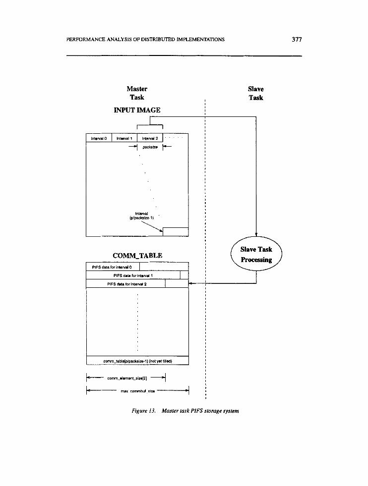
While the slave tasks receive and process the data in this transmission, the master task dynamically allocates an array to store the PIFS information that will be returned by slave tasks and an array that specifies the size of individual PIFS data transmissions. As shown in Figure 13, this storage scheme differs from that of the static allocation system. In this implementation, the input image is divided into intervals containing the number of range blocks per assignment specified by packsize. Thus, an image consisting of p range blocks is partitioned intop/packrize intervals. When the PIFS data for a given interval assignment is returned by a slave task, it is stored in the corresponding row of the dynamic comm-table array. The size (in bytes) of the PIFS data in this row is stored in the comm...elementsize array.

5.2. Dynamic Slave Tasks

The slave task used for this implementation is very similar to that of the static load allocation system. The principal difference between the two implementations is that the new slave task enters a loop in which it can receive multiple assignments before terminating execution, as displayed in Figure 14.

The slave task begins operation by receiving the initialization data from the master task. This includes packsize (which is used to calculate the end co-ordinates of an assignment), user-defined mean square tolerance, and the entire input image. A dynamic array (commbuf), whose size is proportional topacksize, is allocated to store PIFS information. The slave task then uses the initialization data to calculate the Domainavg array and classify all domain blocks.

Next, the task receives the starting z - y co-ordinates of its first assignment. As an assignment is received, the slave task classifies the range blocks and computes PIFS data for that interval, using the algorithm described previously. When the compression of the interval is completed, the resulting PIFS information is copied from the &table structures to commbuf, This buffer is appended with the slave task’s slave task number and the PIFS data size. The resulting data packet is transmitted to the master task.

The slave task then awaits a new assignment from the master task. If the new assignment

376 DAVID JEFF JACKSON AND GREG SCOTT TlNNEY

and Transmit Initial

Unpack PlFS data.

Transmit next assignment in Pool of Tasks to next slave task in queue

-fl Unpack PlFS

data to file

Figure 12. Dynamic master taskjow diagram


Interval 0

Master Task

Interval 1 Interval 2 . . . . .

INPUT IMAGE

comm-table[plpacksire-1 ] (not yet tilled)

I

I I I I I I I I I I I I I I I I I I I I

I I

Slave Task

Interval (plpacksize-1)

COMM-TABLE I PlFS data for intotVal0 I I

PlFS data for interval 1

I I I I I I I I I I I I I I I I I I I I I 1 I I I I I I I I I I I I

Slave Task Processiag

Figure 13. Master task PIFS storage system

378 DAVID JEFF JACKSON AND GREG SCOIT TINNEY

BEGIN 3 initialization

Classify assigned Range blocks

Compress assigned subimage

Pack PlFS data

Transmit results to master task

Figure 14. Dynamic slave taskflow diagram


is an interval of range blocks, the range classification and compression loop is repeated. If, however, the assignment includes the terminate order, the slave task frees its dynamic array, exits from the PVM virtual machine, and terminates.

5.3. Dynamic Load Allocation Results

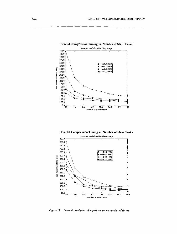
Dynamic load allocation often improves performance in applications with varying loads by more evenly balancing the load between processors. Figure 15 shows that dynamic load allocation does normalize the amount of work performed by each slave task (processor). In this example, no slave task’s total execution time deviates more than 3.1 s from the mean slave task execution time. Deviation that does result is primarily due to the variation in complexity of each slave task’s final assignment. As illustratedin Figure 16, this normalized load considerably improves image compression time, producing average speedups over the optimized sequential implementation of 6.25 for boy.pgm and 9.55 for 1ena.pgm. This corresponds to substantial speedups over the static load allocation system of approximately I .42 for boy.pgm and 1.26 for 1ena.pgm. Note that the execution time for a given RMS tolerance depends on the number of range blocks per assignment @acksize). The smaller the assignment size, the better a parallel system’s load is balanced, because the execution times of the final assignments that cause slave task load imbalance are reduced. However, reducing assignment size also increases the total number of assignments that must be transmitted. Thus, communication overhead is increased. For performance to be optimized, these two factors must be balanced and the best possible packsize chosen. In this research, four range blocks per assignment minimized compression time for boy.pgm, while two range blocks per assignment proved optimal for 1ena.pgm. Note that the appropriate packsize for a given image varies with the specified RMS tolerance and can only be determined through experimentation. In general, however, more complex images require a smaller number of range blocks per assignment, so that deviation in slave task execution time caused by each slave task’s final assignment is minimized.

5.4. Dynamic Load Allocation Conclusions

The results demonstrate that dynamic load allocation is better suited than static load allocation for this parallel fractal image compression algorithm. This is true because dynamic load allocation more evenly distributes the varying load among processors (slave tasks). Thus, until the Pool of Tasks is empty, slave tasks are idle only while awaiting a new assignment from the master task. For less computationally intensive applications, the greater communication overhead required by dynamic load allocation may outweigh the more efficient use of processing power. In this system, however, communication time represents only 0.1 % to 0.7% of the total execution time to compress an image and therefore does not appreciably affect the implementation’s overall performance.

To this point, a virtual machine of 16 RS/6000s was used for all compression tests. It is interesting, however, to investigate the performance of the parallel fractal image compression algorithm for a varying number of host processors. Figure 17 displays the algorithm’s compression time versus the number of slave tasks for several RMS tolerances.

Figure 17 shows that the slopes of the compression time curves approach zero at approximately eight slave tasks for boy.pgm and 12 slave tasks for 1ena.pgm. This leveling-off suggests that a virtual machine of more than the above number of slave tasks (proces-


Slave Task Load Balance

Figure 15. Dynamic load allocation slave load balance

sors) for each image provides little additional performance despite the additional resources applied. In fact, a 16-slave task system does not represent the most efficient performance- to-processor ratio for this particular compression scheme.

6. SP2 PARALLEL SYSTEM IMPLEMENTATION

To address the performance of the implementation in a tightly coupled parallel configuration, the dynamic load allocation code is ported to the SP2 parallel processor. The SP2 utilizes multiple IBM POWER2 microprocessors interconnected via a high performance switch with crossbar topology (full connectivity). A parallel configuration consisting of a single master processor and a variable number of slave processors, 2-10, is employed.

Figure 18 gives compression time versus the number of slave processors for several RMS tolerances. In this case, the dynamic load, distributed to slave processors, is fixed at eight range blocks per assignment. As shown, the performance obtained reflects the general per-

PERFORMANCE ANALYSIS OF DISTRIBUTED IMPLEMENTATIONS 38 1

Parallel Fractal Compression Time vs RMS 16 Processor, dynamic load allocation /boy image

80.0 I , , , , ~ , , I , , , ,

75.0

70.0

65.0

60.0

55.0

6 50.0 5 # 45.0

40.0

35.0

30 0

25.0

m- -m 4 Range blocks ti 2 Range blocks

- - -

- L

2 0 ' o Z 0 3 0 4 0 5 0 6 0 7 0 8 0 90 100 110 120 130 140 1 5 0 user-specified RMS

Parallel Fractal Compression Time vs RMS 16 processor, dynamk load allocation /lena image

140.0

130.0 $+

3 60.0 I

40.0

50.0 1

130.0

120.0

8 110.0 I - 100.0

90.0

- 4 Range blocks ti 2 Range blocks

._ E

2 80.0 0

I a 70.0

3 60.0

50.0

40.0

- 4 Range blocks ti 2 Range blocks

I

I

0

Figure 16. Dynamic load allocation execution times

382 DAVID JFFF JACKSON AND GREG SCO'IT TINNEY

Fractal Compression Timing vs. Number of Slave Tasks dynamic load aNocation /boy image

25.0 -

0.0 ' I 2.0 4.0 6.0 8.0 10.0 12.0 14.0 16.0

number of slaves tasks

Fractal Compression Timing vs. Number of Slave Tasks dynamic load allocation /lena image

A 850.0 800.0 750.0 700.0

H 4.0 RMS ti 3.0 RMS

450.0

350.0

S' 300.0

250.0

200.0

150.0

100.0 - - =

50.0 I-- --_I. I , _.-LI-I

2.0 4.0 6.0 8.0 10.0 12.0 14.0 number of slave tasks

t

1 b

'.O

Figure 17. Dynamic load allocation performance v. number of slaves


0.0 ' I I I

2.0 4.0 6.0 8.0

300.0

275.0

250.0

225.0

h 200.0

- 175.0 150.0

5 125.0

a, 100.0

75.0

50.0

25.0

0 % ._ E 0 .- c

0) x

i 10.0

SP2 Fractal Compression Timing vs. Number of Processors dynamic load allocation I boy image

c

Figure 18. SP2 Dynamic load allocation performance v. number of slaves

formance trend of the distributed workstation implementation. Again, communication time is practically negligible for this implementation. The data suggests, also, that employing over ten additional processors would be of little benefit.

Results obtained show the scalability of the algorithm to a tightly interconnected parallel processor. Performance gain is, however, attributable primarily to an increase in processor power relative to the distributed workstation implementation. Finer-grain decompositions currently being researched [8,9] may demand high performance interconnectivity as an image, and thus domain blocks may be distributed across many processors. However, for the coarse-gain implementations presented, in which an entire source image may reside at each processor, the problem remains computationally bound.


t - t Boy image (Fractal) + - ~ + Boy image (JPG) M Lena image (Fractal) .4 - - A Lena image (JPG)

10.0 0.0 10.0 20.0 30.0 40.0

Compression Ratio

Figure 19. SNR versus compression ratio

7. FRACTAL VERSUS JPEG COMPARISON

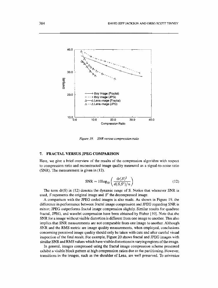
Here, we give a brief overview of the results of the compression algorithm with respect to compression ratio and reconstructed image quality measured as a signal-to-noise ratio (SNR). The measurement is given in (12).

The term dr(S) in ( 1 2) denotes the dynamic range of S. Notice that whenever SNR is used, S represents the original image and S' the decompressed image.

A comparison with the JPEG coded images is also made. As shown in Figure 19, the difference in performance between fractal image compression and JPEG regarding SNR is minor; JPEG outperforms fractal image compression slightly. Similar results for quadtree fractal, JPEG, and wavelet compression have been obtained by Fisher [lo]. Note that the SNR for a image without visible distortionis different from one image to another. This also implies that SNR measurements are not comparable from one image to another. Although SNR and the RMS metric are image quality measurements, when employed, conclusions concerning perceived image quality should only be taken with care and after careful visual inspection of the final result. For example, Figure 20 shows fractal and JPEG images with similar SNR and RMS values which have visible distortions in varying regions of the image.

In general, images compressed using the fractal image compression scheme presented exhibit a visible block pattern at high compression ratios due to the partitioning. However, transitions in the images, such as the shoulder of Lena, are well preserved. To minimize


SNR=34.04 RMS=4.98

SNR=32.23 RMS=5.15

SNR=32.18 RMS=5.76

SNR=33.26 RMS=5.10

(a) JPEG images

Figure 20.

(b) FRACTAL images

Fractal and JPEG SNR comparisons for test images

the artifacts along the partition boundaries, the image can be postprocessed as a part of the decompression algorithm [5 ] . Images compressed using JPEG show only littlevisible block patterns at moderate compression ratios. However, transitions are blurred and distorted due 1.0 the missing content of high frequencies. Thus, future research directed towards a fractal- JPEG hybrid compression scheme seems promising.


8. CONCLUSIONS

Fractal image compression utilizes the affhely redundant nature of images and the fractal transform to encode a bitmap as the union of several smaller, non-overlapping attractors. Because of the extensive affine redundancy of many images, one author suggests that fractal image compression techniques can be applied to an image to obtain lossy compression ratios in excess of 10,OOO:l [ 13. Current implementations, however, show fractal compression to be similar in compression ratio and image quality to JPEG. The major limitation of fractal image compression is its computational complexity. Because of the large number of expensive range-domain comparisons required to encode an image, the fractal transform’s compression time is considerably longer than that of present lossy compression standards such as JPEG. Because of the independent nature of encoding range blocks, however, the fractal transform responds well to implementation on a distributed system. Another important strength of the fractal image compression scheme is its computationally simple decoding, an attractive component for image archival.

The fractal compression algorithm presented is shown to perform well in a coarse-grain distributed system with a dynamic load distribution approach. The implementation is partic- ularly effective due to low communication overhead and the effectiveness of the simplistic master/slave programming model employed. Future implementation considerations, and current research efforts, include an adaptation of the algorithm for execution on a more highly parallel architecture, with appropriate architectural considerations.

REFERENCES 1. M. F. Barnsley and A. D. Sloan, ‘A better way to compress images,’ Byte, 215-223 (January

1988). 2. B. B. Mandelbrot, The Fractal Geometry of Nature, W. H. Freeman and Company, New York,

3. L. F. Anson, ‘Fractal image compression,’ Byte, 195-202 (October 1993). 4. M. F. Barnsley and L. P. Hurd, Fractal Image Compression, AK Peters, Ltd., Wellesley, Mas-

sachusetts, 1993, pp. 1-188. 5. Y. Fisher, ‘Fractal image compression,’ SIGGRAPH ‘92 Course Notes, 1992. 6. A. E. Jacquin, ‘Image coding based on a fractal theory of iterated contractive image transforma-

tions,’ IEEE Trans. Image Process, 1, (l), 18-30 (1 992). 7. A. Geist et al, (Eds.), PVM 3.0 User’s Guide and Reference Manual, Oak Ridge National

Laboratory, Oak Ridge, Tennessee, 1993, pp. 1-3 1. 8. David J. Jackson and Thomas Blom, ‘Fractal image compression using a circulating pipeline

computation model,’ Technical Report UA-CARL-95-DJJ-01, Computer Architecture Research Laboratory, The University of Alabama, March 1995.

9. David J. Jackson and Thomas Blom, ‘A parallel fractal image compression algorithm for hyper- cube multiprocessors,’ Proceedings of The Twenty-Seventh Southeastern Symposium on System Theory, 12-14 March 1995, pp. 274-278.

10. Y. Fisher, D. Rogovin and T.P. Shen, ‘A comparison of fractal methods with dct (ipeg) and wavelets (epic),’ SPIE Proceedings, Neural and Stochastic Methods in Image and Signal Pro- cessing Ill, vol. 2304-1 6, San Diego, CA, 28-29 July, 1994.

1 9 8 3 , ~ ~ . 1-15.

Documents

Performance analysis of distributed implementations of a fractal image compression algorithm