Embed Size (px)
Citation preview

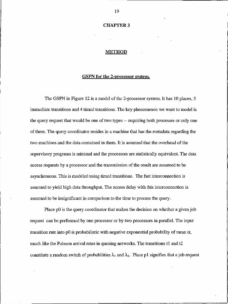
Performance analysis of multiprocessor systems in a distributed large data set model using generalisedstochastic petri netsby L Shrihari
A thesis submitted in partial fulfillment of the requirements for the degree of Master of Science inComputer ScienceMontana State University© Copyright by L Shrihari (1995)
Abstract:A method is proposed for the study of performance characteristics of a 2 or 3 processor homogenousparallel data server system where the individual processors have unique access to statically ordynamically partitioned data in a very large data set using Generalized Stochastic Petri Nets. very largedata sets or a warehouse of data can be partitioned and the operations can be done in parallel enhancingtheir time of completion. Parameters observed in this distributed data environment with multiprocessorarchitectures have been the effect of mixture of queries that exhibit varying degrees of data parallelism.The scheduling of the mixture of queries is non-adaptive in the case of statically partitioned data andwould be adaptive in the case of dynamically partitioned data. The system studied is one in whichqueries predominate and the information in the servers is updated at specific times where queries arenot permitted. Hence, serializability of transactions - as most of them are queries - is not part of thismodel. A simulator was written to study the Petri Net models and the performability of the differentnets with different mixtures of parallel queries. The results clearly show that the architecture chosen isscalable as the data grows and does show the necessity on the part of the analyst to partition data on atimely basis to enhance performance.

PERFORMANCE ANALYSIS OF MULTIPROCESSOR SYSTEMS IN A DISTRIBUTED LARGE DATA SET MODEL USING GENERALISED
STOCHASTIC PETRI NETS.
by L. Shrihari
A thesis submitted in partial fulfillment of the requirements for the degree
of
Master of Science
in
Computer Science
MONTANA STATE UNIVERSITY Bozeman, Montana
September 1995

u
APPROVAL
of a thesis submitted by
L Shrihari
This thesis has been read by each member of the thesis committee and has been found to be satisfactory regarding content, English usage, format, citations, bibliographic style, and consistency, and is ready for submission to the College of Graduate Studies.
uate Committee
Date
Approved for the Major Department
'nTT^ -—>Hedd, Major Department 4
Approved for the College of Graduate Studies
Graduate Dean

m
STATEMENT OF PERMISSION TO USE
In presenting this thesis in partial fulfillment of the requirements for a master’s
degree at Montana State University, I agree that the Library shall make it available to
borrowers under rules of the Library.
If I have indicated my intention to copyright this thesis by including a copyright
notice page, copying is allowable only for scholarly purposes, consistent with “fair use”
as prescribed by the U.S. Copyright Law. Requests for permission for extended
quotation from or reproduction of this thesis in whole or in parts may be granted only
by the copyright holder.
Signature
Date

iv
To my teachers with thanks.
V
TABLE OF CONTENTS
LIST OF FIG U R ES............................................................................................................ vi
A B S T R A C T ...................................................................................................................... viii
1. IN TRO D U C TIO N .......................................................................................................... IM otivation..................................................................... ILimitations of the Uniprocessor M odel................................................................. 2
Architectures of Parallel Data S e rv e rs ................................................................... 3DBMS Strategies for Parallel Data Servers.......................................................... 5Stochastic M odeling........................................ 6
2. PETRI NETS - B A C K G R O U N D ................................................................................. 8Definition - Petri N e ts .............................................................................................. 8Definition - Inhibitor N e t ....................................................................................... 10Power of Petri N e ts .................................................................................................... 11Stochastic Petri N e ts ................................................................................................. 15Definition - S P N ......................................................................................................... 16Generalized Stochastic Petri Nets............................................................................ 16
3. M ETH O D .......................................................................................................................... 19GSPN for the 2-processor sy s te m .......................................................................... 19GSPN for the 3-processor system .......................................................................... 22Im plem entation............................................................................................................ 26R esu lts ........................................................................................................................ 30Limitations of the current models and suggestions for future research . . . . . . . 35
BIBLIOGRAPHY 36

LIST OF FIGURES
Figure Page
1. Shared Everything A rch itectu re .......................................................... ................... 4
2. Shared Nothing A rch itectu re ...................... ............................................................ 4
3. Before transition t l f ire s ............................................................................................ 9
4. After transition t l f i r e s .............................................................................................. 9
5. Sequential execution................................................................................................... 11
6. Concurrency................................................................................................................. 12
7. C o n flic t........................................................................................................................ 12
8. M erging........................................................................................................................ 13
9. Synchronization.............................................................................. 13
10. Priorities/Inhibitions............................................................................ 14
11. Immediate transition t l and exponential transition t 2 .......................................... 17
12. GSPN model of the 2-processor system ................................................................. 20
13. GSPN model of the 3-processor system ................................................................. 23
14. GSPN model of the 3-processor system (contd)........... : ..................................... 24
15. GSPN model of the 3-processor system (contd)................................................... 25
16. Implementation scheme of the G SP N ........................................ 26
17. The grammar for the INPUT-NET.......................................................................... 27
vi
LIST OF FIGURES (continued)
Figure Page
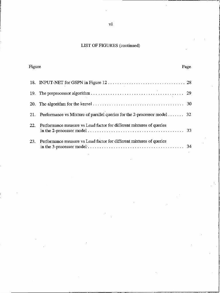
18. INPUT-NET for GSPN in Figure 1 2 ........................................................................ 28
19. The preprocessor algorithm ....................................................................................... 29
20. The algorithm for the kernel..................................................................................... 30
21. Performance vs Mixture of parallel queries for the 2-processor m odel............. 32
22. Performance measure vs Load factor for different mixtures of queriesin the 2-processor m odel.......................................................................... 33
23. Performance measure vs Load factor for different mixtures of queriesin the 3-processor m odel.................................................. 34

viii
ABSTRACT
A method is proposed for the study of performance characteristics of a 2 or 3 processor homogenous parallel data server system where the individual processors have unique access to statically or dynamically partitioned data in a very large data set using Generalized Stochastic Petri Nets. Very large data sets or a warehouse of data can be partitioned and the operations can be done in parallel enhancing their time of completion. Parameters observed in this distributed data environment with multiprocessor architectures have been the effect of mixture of queries that exhibit varying degrees of data parallelism. The scheduling of the mixture of queries is non- adaptive in the case of statically partitioned data and would be adaptive in the case of dynamically partitioned data. The system studied is one in which queries predominate and the information in the servers is updated at specific times where queries are not permitted. Hence, serializability of transactions - as most of them are queries - is not part of this model. A simulator was written to study the Petri Net models and the performability of the different nets with different mixtures of parallel queries. The results clearly show that the architecture chosen is scalable as the data grows and does show the necessity on the part of the analyst to partition data on a timely basis to enhance performance.

I
CHAPTER I
INTRODUCTION
Motivation
Most real world applications and the data associated with them have special
characteristics that warrant fine tuning in logical and/or physical design of the data store
to get speedier answers to queries. Proper logical design such as assignment of
relationships through foreign keys or indexes, unique indexes and constraints that tend to
model domains enhance performance in most database management systems (DBMS);
such gains cannot be significant in a very large data set or data warehouse.
Data warehousing refers to the collection, manipulation, distribution and
information processing of very large amounts of data. The data store or database could be
from many gigabytes to a few terabytes. Data of this magnitude is usually historical in
nature; it was collected over a period of time. Decision Support Systems (DSS), where
the knowledge of an enterprise resides, are usually data warehouses that span a large
period of time, usually years. With very large amounts of data the warehouse could be a
good prognosticator of trends in various meta-models such as retailing, lottery trends,
employment statistics, consumer trends, and insurance and actuarial systems.
Retrospective analysis of how a business was run and the clues on the profitability of long

2
range decisions will yield insights into the causal effect of many decisions. Companies and
institutions have been waiting for cheaper technologies that could harness all their
non-operational data — data that is not used for day to day operations — into information.
The cost of such information, that is, a transformation of historic data into useful
knowledge, is usually very high. Special proprietary systems exist that are prohibitively
expensive, leading to the high cost of processing information.
The advent of inexpensive hardware configurations in the form of ever more
powerful processors, cheaper and faster memory and media, the declining price to
performance ratios, and the vendors’ quest to support open and non-proprietary operating
systems, database systems, and tools, are important reasons to look into data-warehousing
solutions for DSS.
Lim itations O f The Uniprocessor Model
The uniprocessor approach of sequential execution has been the most widely used
architecture for database solutions. The performance of this model is limited to the speed
of the processor and the usual disk I/O time. The limitations are:
o The uniprocessor architecture is unsuited for a large data set that has data widely
spread over time. The data has latent parallelism that is unused by the uniprocessor
model.
o The relational database systems tuned to the multiprocessor approach does lead to
more parallelism based on the query.
3
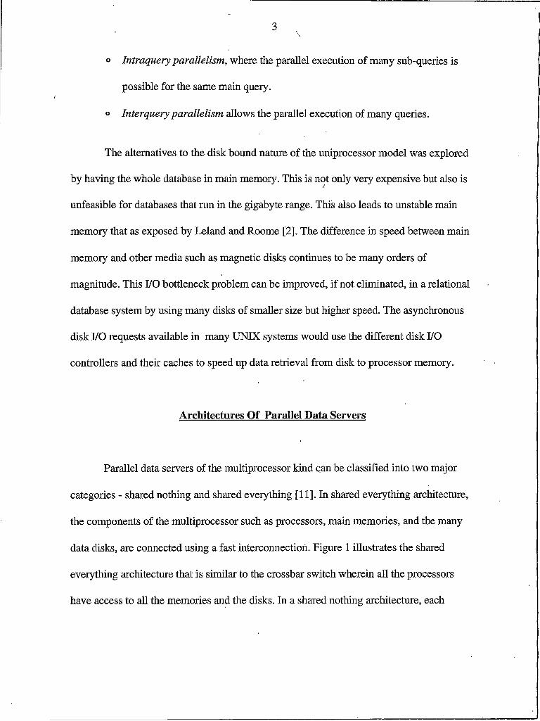
o Intraquery parallelism, where the parallel execution of many sub-queries is
possible for the same main query.
o Inter query parallelism allows the parallel execution of many queries.
The alternatives to the disk bound nature of the uniprocessor model was explored
by having the whole database in main memory. This is not only very expensive but also is
unfeasible for databases that run in the gigabyte range. This also leads to unstable main
memory that as exposed by Leland and Roome [2]. The difference in speed between main
memory and other media such as magnetic disks continues to be many orders of
magnitude. This I/O bottleneck problem can be improved, if not eliminated, in a relational
database system by using many disks of smaller size but higher speed. The asynchronous
disk I/O requests available in many UNIX systems would use the different disk I/O
controllers and their caches to speed up data retrieval from disk to processor memory.
Architectures Of Parallel Data Servers
Parallel data servers of the multiprocessor kind can be classified into two major
categories - shared nothing and shared everything [11]. In shared everything architecture,
the components of the multiprocessor such as processors, main memories, and the many
data disks, are connected using a fast interconnection. Figure I illustrates the shared
everything architecture that is similar to the crossbar switch wherein all the processors
have access to all the memories and the disks. In a shared nothing architecture, each

4
processor has exclusive access to memories and disks. Figure 2 shows the shared nothing
model that is similar to the switch based multiprocessor.
FAST INTERCONNECTION
PROCESSORS MEMORIES DISKS
Figure I . Shared Everything Architecture.
FAST INTERCONNECTION
PROCESSORS
MEMORIES
DISKS
Figure 2. Shared Nothing Architecture.

5
DBMS strategies for Parallel Data Servers
Traditionally, shared nothing models are associated with static partitioning of data,
and the shared everything models, with dynamic partitioning of data. Static partitioning
entails the fragmentation of data across multiple disks that are available to only one
processor at all times. Query decomposition is hence dependent on where the data resides
and not on the processor availability. This leads to the need for the system analyst to re
partition data that is contended by more user queries on a continual basis, to avoid
unbalanced parallelism. However, this model is very extensible; the growth in data can be
supported by growth in the number of processors. Examples of shared nothing servers are
Tandem NonStop SQL and Teradata DBC/1012.
In dynamic partitioning — associated with shared everything models — there is
no need for repartitioning data. The processors have access to all the disks and the
available processors deal with the next request and have access to requests. In this model
the requests made by users do not wait for the appropriate processor that has a hold on
the data, but make do with the processor that is available. Efficient usage of CPU and the
lack of need to anticipate the partitioning methods are the primary advantages of this
model. Examples of shared everything servers are machines from Sequent, data servers
from XPRS and the SABRE data server.

6
Stochastic Modeling
To measure performance of a system the designers can perform measurement tests
on the actual system or use prototypes which emulate the system under different
conditions and artificial workloads. Both of these are very involved tasks requiring the
design to be mature or complete. The availability of a system or a complete design both at
the hardware and software levels is important for measurement testing or for prototyping
the system. These conditions are not possible in most real projects.
The study of the behavior and performance of a system can be done in an easier
fashion by simulation modeling or through analytical methods. Such studies could be
either deterministic or probabilistic. Simulation models can be constructed through
modeling tools or by writing programs using a high level language. Analytical models are
mathematical descriptions of the behavior of the system. For both of these to be successful
the designers need to specify a level of abstraction at all levels of the system — hardware,
software, and applications.
Simulation modeling using probabilistic estimates of the behavior is a possible
abstraction of a complex system. Such broad assumptions could allow the designers to
focus on the significant aspects of the system omitting the various minute details, which
lead to unnecessary complexity in the model. Also, when the level of abstraction is
adequate to represent the system, it is easier to observe the differences with changes in the
overall design of the system.

7
Generalized Stochastic Petri Nets provide a sound and convenient method to
analyze and validate design approaches. A number of commercial packages exist that have
easy-to-use graphical user interfaces that model stochastic petri nets.
8
CHAPTER 2
Petri Nets — Background
Petri Nets (PNs) or place-transition nets, are bipartite graphs first proposed in
1962 by Carl A. Petri. They are methods for modeling concurrency, nondeterminism,
synchronization and control flow in systems. What follows is a cursory introduction; for
detailed definitions and rigorous mathematical proofs please refer to [12, 13].
Definition — Petri Net
A PN is a set of places P, a set of transitions T, and a set of directed arcs A.
The graphical schematic representation of PNs is places as circles and transitions as bars
(horizontal or vertical lines). Transitions are connected to and from places by directed
arcs. Black dots within a place are called tokens. The state of a PN is the number of
tokens in each place, called a marking. The definition of a PN is not complete without the
specification of the initial marking M0
Formally, a PN is a quintuple ( P, T, INPUT, OUTPUT, M0 ) where
P = { p i, p2, p3, . . . , pn } is the set of n places.
T = { t], t2, t3, ... , tm } is the set of m transitions.
P u T (j) and P n T = ([>
INPUT : ( P x T ) —» PTi is an input function that describes directed arcs from places to transitions.
OUTPUT : ( P x T ) —> TPi is an output function that describes directed arcs from transitions to places.
M0 = { m i, m2, m3, . . . , mn } is the initial marking.
9
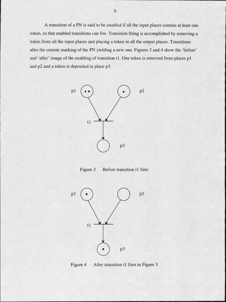
A transition of a PN is said to be enabled if all the input places contain at least one
token, so that enabled transitions can fire. Transition firing is accomplished by removing a
token from all the input places and placing a token in all the output places. Transitions
alter the current marking of the PN yielding a new one. Figures 3 and 4 show the ‘before’
and ‘after’ image of the enabling of transition tl. One token is removed from places p i
and p2 and a token is deposited in place p3.
Figure 3 Before transition tl fires
Figure 4 After transition tl fires in Figure 3

10
Formally, a transition tj is said to be enabled in a marking M if
M(pi) > INPUT(pi, tj) for all pi e set of all places from whom adirected incoming arc reaches tj.
An enabled transition tj can fire at any time. When a transition tj is enabled in a
marking Mi, it fires, resulting in a new marking M2, according to the equation
M2(Pi) = Mi(pi) + OUTPUT(pi,tj) - INPUT(pi,tj) for all Pi e P ... (I)
Marking M2 is reachable from M 1 when transition tj is fired. Every marking is considered
to be reachable from itself by enabling no transition. If some marking Mj is reachable from
Mi and Mk is reachable from Mj, then it follows that Mk is reachable from Mi. Reachability
of markings exhibit transitive and reflexive relations. The set of all markings reachable
from the initial marking Mo is the reachability set R(Mo).
Definition - Inhibitor Net
An inhibitor net is a 6-tuple ( P, T, INPUT, OUTPUT, INHIB , Mo) where ( P, T,
INPUT, OUTPUT ,Mo) is a PN and
INHIB : ( P x T ) -» {0, 1}
is an inhibitor function. In an inhibitor net, a transition tj is enabled in a marking M if
M(pi) > INPUT ( pi, t j ) for all pi G { set of all places from whom anincoming arc reaches tj }, and .
M(pi) = 0 for all pi for which INHlB( pi, Ij ) ^ 0.
On firing tj, the new marking is obtained from equation (I).
11
Power of Petri Nets
Common activities that can be modeled are concurrency, decision making,
synchronization and parallelism, priorities, conflicts and confusion. PN constructs allow
representation of many different activities that are not easily represented in finite state
machines, such as concurrency and synchronization. Marked graphs can model
concurrency and synchronization but cannot model conflicts and merging. The
representational power of the PNs is best understood graphically. The most common
primitives are given below with their corresponding figures.
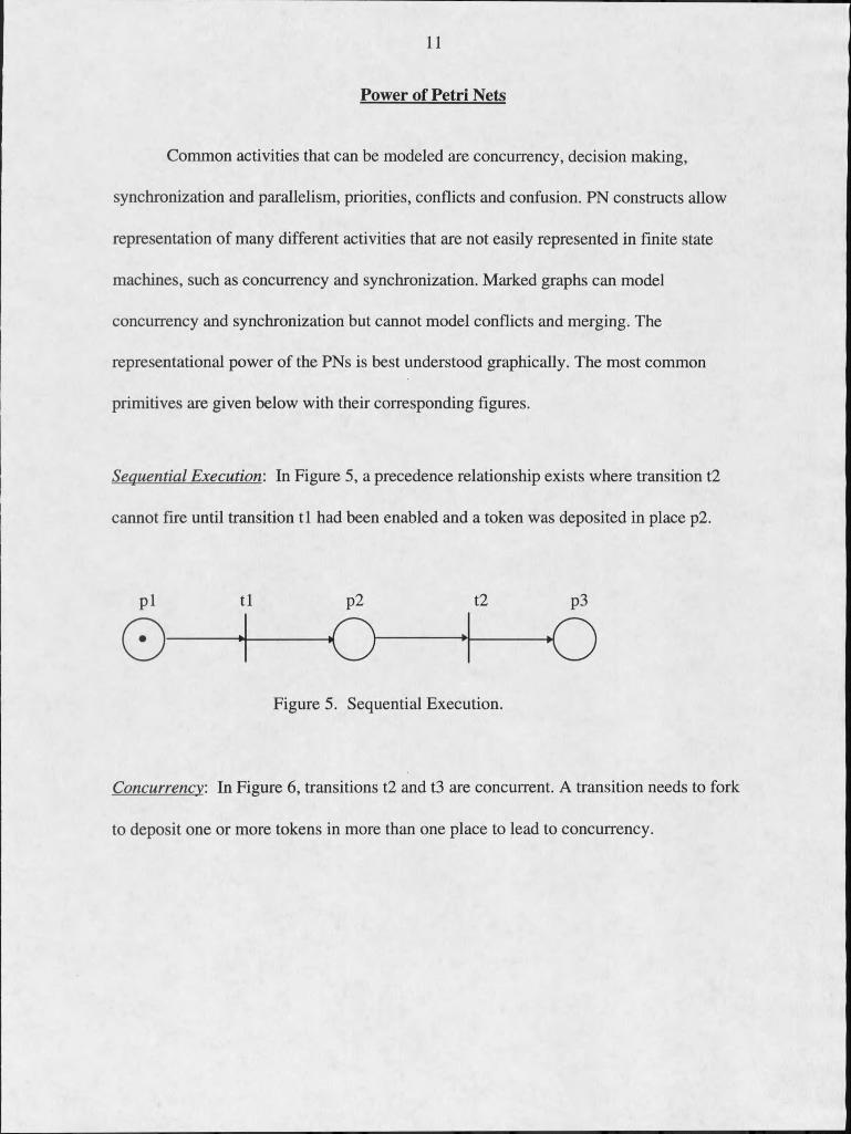
Sequential Execution: In Figure 5, a precedence relationship exists where transition t2
cannot fire until transition tl had been enabled and a token was deposited in place p2.
p i tl p2 t2 p3
Figure 5. Sequential Execution.
Concurrency: In Figure 6, transitions t2 and t3 are concurrent. A transition needs to fork
to deposit one or more tokens in more than one place to lead to concurrency.

12
p2 t2
FORK
Figure 6. Concurrency.
Conflict'. In Figure 7, transitions tl , t2 and t3 are in conflict. All transitions are enabled,
leading to nondeterminism. This is common in systems where a condition or activity leads
to a choice. This situation could be resolved by the assignment of probabilities for the
transitions t l , t2 and t3.
Pi
Figure 7. Conflict.
Merging: In Figure 8 transitions tl and t2 merge. This is a classic join operation where
different activities lead to the same state or condition. Together with the fork and join it
would be easy to model the parbegin-parend construct of Djikstra.

13
tl t2
JOIN
t3
Figure 8. Merging.
Synchronization: When the culmination of one or more events in a system is to be waited
on then we need a synchronization construct. Figure 9 shows the need to wait until place
p i gets a token. Transition tl will not be enabled until the token arrives in place p i.
Figure 9. Synchronization.

14
Priorities/Inhibitions: The classical PN definition as given by Petri cannot model
priorities. However the extended definition of the inhibitor net will allow priorities. An
inhibition is marked from a place to a transition not as a directed arc but as a line that ends
with a bulb at the transition.
Figure 10 shows a transition that inhibits the enabling of the transition if there is a
token in place p2. In the illustration the transition to be enabled is 11. If there was no
token in p2 then the PN results in conflict that must be resolved by a switching distribution
in a probabilistic manner.
p i p2
Figure 10. Priorities/Inhibitions.
Inhibitor arcs enhance the modeling power of the PN model. It has been shown
that PNs with inhibitor arcs are equivalent to Turing machines [12]. It has also been
proven that the original PNs are less powerful than Turing machines and can only generate
a proper subset of context-sensitive languages.

15
Classical PNs are useful in investigating qualitative or logical properties of
concurrent systems, such as safeness, resource allocation or conservation, mutual
exclusion, absence of deadlocks or their existence, reachability and study of the states of
the system. They are, however, not very suitable for quantitative analysis of systems.
Stochastic Petri Nets
To enhance the quantitative features of PNs the concept of time was needed in the
definition of PNs. The idea of introducing time into a PN is based on the idea that for a
system model in a given marking (state), a certain amount of time-must have elapsed
before an event occurs. The result of some activity in a given state is thus tracked by time.
Ramamoorthy and Ho [11] investigated the use of Timed Petri Nets (TPN)in which
places or transitions were incorporated with deterministic (constant) time delays. The
analysis of such TPNs was found intractable in most cases except where the PN was
equivalent to a marked graph.
The doctoral dissertations of S. Natkin [9] and M. K. Molloy [8] independently
led to Stochastic Petri Nets (SPNs), where they associated exponentially distributed
random delays to transitions. These methods are isomorphic to Continuous Time Markov
Chains (CTMCs). Each marking of an SPN is equivalent to a state of the CTMC. SPNs
suffered from graphical and analytical complexity as the systems to be modeled increased
in size and complexity. The number of states of the CTMC along with the SPN
reachability set exploded, rendering SPNs to be used for modeling systems of smaller size
and complexity.

16
Definition - SPN
An SPN is a 6-tuple ( P, T, INPUT, OUTPUT, M0, F ) where ( P, T, INPUT,
OUTPUT, M0) is the marked untimed PN and F is a function in the domain of the
cartesian product of the reachability set and the transitions ( R[M0] x T ), which associates
with each transition in each reachable state, a random variable.
Every transition has a firing delay associated with its action. This is the time that
will elapse before the transition can fire. The firing delay is a random variable with a
negative exponential probability distribution function.
Generalized Stochastic Petri Nets
Generalized Stochastic Petri Nets (GSPNs), proposed by Marsan, Balbo and
Conte [3,4, 5] allow the firing delays to be zero or the transition to be fired immediately.
GSPNs are obtained by allowing transitions to belong to two different classes: immediate
transitions and exponential transitions. Immediate transitions fire in zero time once they
are enabled. Exponential transitions are fired in exponentially distributed firing times. The
immediate transitions have priority over timed transitions. It is important to note that
associating no time with some transitions enhances the qualitative modeling of a system.
Time is associated with only those transitions that have a larger (time-wise) impact in the
modeled system. The availability of a logical structure that can be used along with the

17
timed activities allows the construction of elegant performance models of complex
systems.
Formally, a GSPN is an 8-tuple ( P, T, INPUT, OUTPUT, INHIB, M0, F, S ) where
• ( P, T, INPUT, OUTPUT, INHIB, M0 ) is an inhibitor-marked PN,
• T is partitioned into two sets: T imm of immediate transitions and TEXp of
exponential transitions,
• F: ( R[M0] x Texp ) —> R is a firing function associated with each t e
Texp each M G R[M0], an negative exponential random variable with rate F (
M, t ) ,
• Each t e Timm has zero firing time in all reachable markings, and
• S is a set, possible empty, of elements called random switches, which associate
probability distributions to subsets of conflicting immediate transitions.
Exponential transitions are drawn as rectangular (filled or unfilled) bars or
segments. All other graphical notations are the same as those of PNs. Figure 11 shows the
immediate transition tl and the exponential transition t2.
tl p2 t2 p3
Figure 11. Immediate transition tl and exponential transition t2.

18
In a GSPN marking, more than one transition can be enabled at one time. If Mi is a
reachable marking and if Ti is the set of enabled transitions in Mi, then Ti includes only
exponential transitions. The transition tj e Ti fires with probability
F ( Mi, tj)
P { tj } = ________ :_______
I F ( Mi, tk )
tk G T imm
If Ti consists of only one immediate transition tj, then tj will fire. If Ti consists of two or
more immediate transitions, then a probability mass function is specified on the set of
enabled immediate transitions by a member of S. The enabled transition is chosen
according to this probability distribution. The set of all immediate transitions, together
with the switching distribution of these transitions is called the random switch. The
probabilities in a switching distribution could be independent of the current marking {static
random switch) or dependent on the current marking {dynamic random switch).
The GSPN model assumes that transitions are fired one by one, even if all the
transitions that could be enabled constitute a set of nonconflicting immediate transitions.
This simplifies the implementation of these models.
A GSPN marking which enables only timed transitions is called a tangible marking
and one which enables at least one immediate transition is called a vanishing marking. It is
imperative on the part of the designer of the net to decide on a semantic policy for the
execution of the net [6, 7].
19
CHAPTER 3
METHOD
GSPN for the 2-processor system.
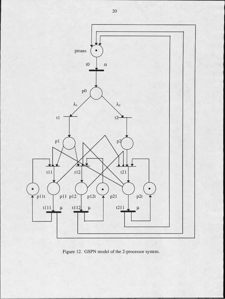
The GSPN in Figure 12 is a model of the 2-processor system. It has 10 places, 5
immediate transitions and 4 timed transitions. The key phenomenon we want to model is
the query request that would be one of two types — requiring both processes or only one
of them. The query coordinator resides in a machine that has the metadata regarding the
two machines and the data contained in them. It is assumed that the overhead of the
supervisory programs is minimal and the processors are statistically equivalent. The data
access requests by a processor and the transmission of the result are assumed to be
asynchronous. This is modeled using timed transitions. The fast interconnection is
assumed to yield high data throughput. The access delay with this interconnection is
assumed to be insignificant in comparison to the time to process the query.
Place pO is the query coordinator that makes the decision on whether a given job
request can be performed by one processor or by two processors in parallel. The input
transition rate into pO is probabilistic with negative exponential probability of mean a ,
much like the Poisson arrival rates in queuing networks. The transitions t l and t2
constitute a random switch of probabilities Xi and X2. Place p i signifies that a job request
20
ptrans
p l l p l2
Figure 12. GSPN model of the 2-processor system.
21
from pO is a one-processor job and place p2 signifies that a job request from p2 is a
2-processor one.
The associated delay rates Xj and X2 of the random switch mean that place p i will
have probability ( Xi / ( Xi + X2 )) of receiving a token or getting a job request from pO,
and place p2 will have probability ( X2 /( Xi + X2 )). If the sum of the two values is set to
one, we would have normalized values for the random switch. The places p i I, p 12 and
p21 are places where the individual processors (in the case of p i I and p i 2) or both ( in
the case of p21) are working in their private memories. The places p i It, p l2 t and p21t
are to signify that the processors are available for processing. So when a token is in p i,
the presence of a token in p i It or p i2 t would mean that both the processors are idle and
that either one could be assigned the request. If p l2 t has no tokens — processor 2 is busy
— then p i I is the only choice. Place p21 has an input transition which is also inhibited by
the places p i I and p l2 . The 2-processor request cannot go further if both or one of the
processors is busy. Transitions t i l l , t l l 2 and t211 are timed transitions that model the
processing times of the job request with a delay rate of mean p. and they are assumed to be
distributed in a exponential distribution. This would be a stochastic approximation of the
internal details of database accesses, the processing of data and the transmission occurring
through a fast interconnect. The measure of the load factor on the system could be
characterized as the ratio of a by |U.
22
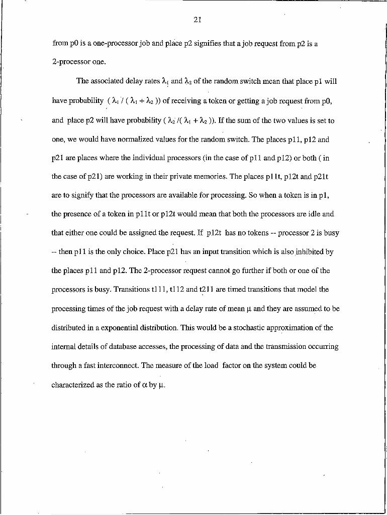
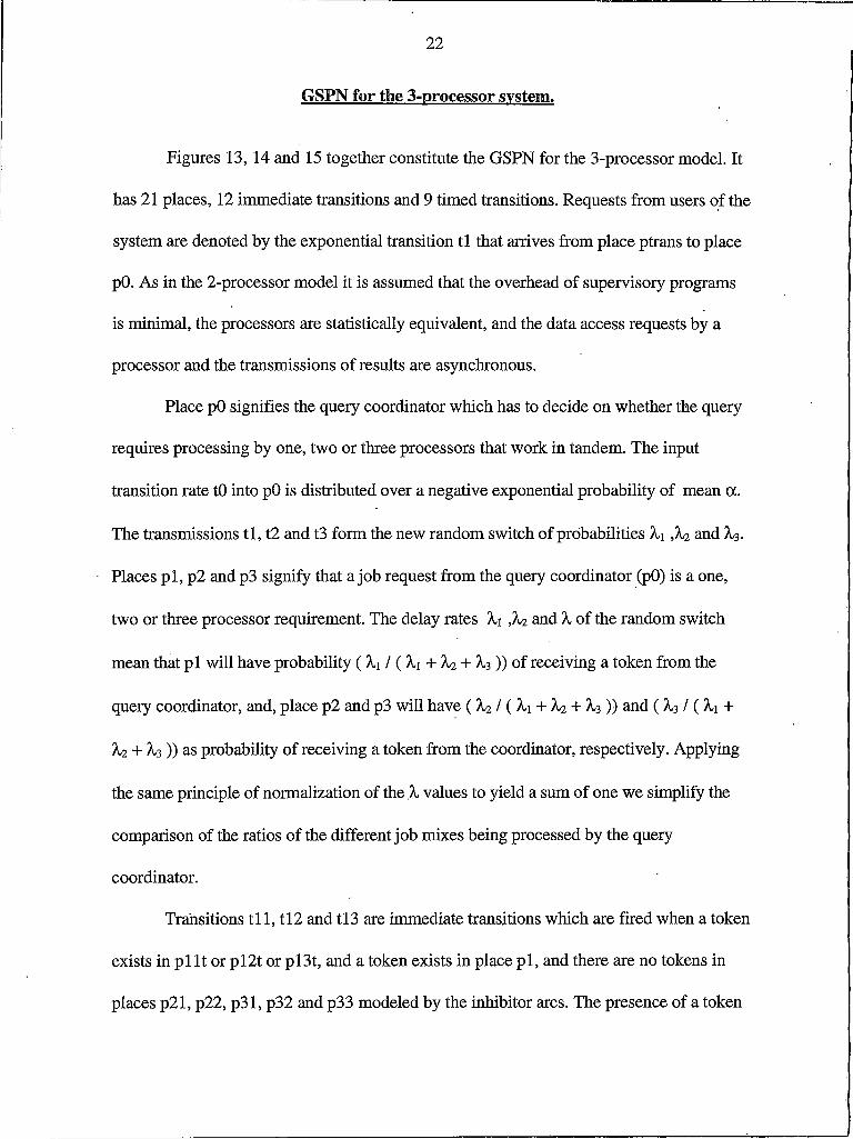
GSPN for the 3-processor system.
Figures 13, 14 and 15 together constitute the GSPN for the 3-processor model. It
has 21 places, 12 immediate transitions and 9 timed transitions. Requests from users of the
system are denoted by the exponential transition t l that arrives from place ptrans to place
pO. As in the 2-processor model it is assumed that the overhead of supervisory programs
is minimal, the processors are statistically equivalent, and the data access requests by a
processor and the transmissions of results are asynchronous.
Place pO signifies the query coordinator which has to decide on whether the query
requires processing by one, two or three processors that work in tandem. The input
transition rate tO into pO is distributed over a negative exponential probability of mean a .
The transmissions t l , t2 and t3 form the new random switch of probabilities ,X2 and X3.
Places p i, p2 and p3 signify that a job request from the query coordinator (pO) is a one,
two or three processor requirement. The delay rates Xi ,X2 and X of the random switch
mean that p i will have probability ( Xi / ( X1 + X2 + X3)) of receiving a token from the
query coordinator, and, place p2 and p3 will have ( X2 / ( X1 + X2 + X3 )) and ( X3 / ( X1 +
X2 + X3)) as probability of receiving a token from the coordinator, respectively. Applying
the same principle of normalization of the X values to yield a sum of one we simplify the
comparison of the ratios of the different job mixes being processed by the query
coordinator.
Transitions t i l , t l2 and tl3 are immediate transitions which are fired when a token
exists in p i It or p l2 t or p l3 t, and a token exists in place p i, and there are no tokens in
places p21, p22, p31, p32 and p33 modeled by the inhibitor arcs. The presence of a token

23
ptrans
ptrans ptrans ptrans
Figure 13. GSPN model of the 3-processor system.

24
ptransptrans ptrans
Figure 14. GSPN model of the 3-processor system (continued).
in places p i It, p i2 t and p l3 t implies the availability of the individual processors. The
timed transitions t i l t , tl2 t and tl3 t model the time taken by the processors to complete
the query request. They have a delay of Ji associated with them.
Place p2 could receive a token from pO based on the random static switch. A token
can be placed in place p21 if and only if places p i I and p l2 do not have a token in them —
they are the processors that are used for this 2-processor query — and place p2t has a

25
ptrans ptrans ptrans
Figure 15. GSPN model of the 3-processor system (continued).
token in it. Since there cannot be more than one 2-processor request in a 3-processor
combination at any one time, the absence of a token in p2t will mean that any two
processors are busy and no other 2-processor queries can be entertained at that time.
Place p3 in Figure 15 is similar to place p2 in Figure 14, with the essential
difference that it models the 3-processor request. A token could be put in place p3 from
place pO by way of the random switch. A token can result in place p31 from place p3 if
there are no tokens in places p21 and p l3 and there exists a token in place p3t. There

26
cannot be tokens in places p31, p32 and p33 at the same time as the number of requests
through the system are served on a First Come First Served (FCFS) basis. This is
characterized by having only one token in the initial marking of the net for place p3t so at
any time there can be only one 3-processor request.
Implementation
Figure 16 illustrates the architecture of the implementation of the GSPNs in Figures 12
through 15. Again the measure of the load factor is characterized by the ratio of a by p,.
< INPUT NET >
GSPN preprocessor
< Firing functions and Data Definitions >
GSPN Kernel Source
< GSPN Executable Instance for this INPUT NET>
Figure 16. Implementation scheme of the GSPN.

27
The schematic GSPN is written out in the form of an INPUT-NET using the
grammar in Figure 17.
Firing Functions and Data Definitions = START definitions END definitions = NULL I definitions placedefns I definitions transdefns placedefns = PLACELIST placelist PLACEEND transdefns = TRANSLIST translist TRANSEND placelist = place I place placelist place = PLACE NAME markings = value translist = transition I transition translist transition = TRANS name type = value rate = value
INPUT ilist OUTPUT olist INHIB Mist ilist = NULL I ilist nameolist = NULL I olist namehlist = NULL I Mist namename = [ A-Za-z] [A-Za-z0-9_] *value = [-+.0-9edEd]+
Figure 17. The grammar for the INPUT-NET.
The reserved words used in the grammar are START, END, PLACELIST,
PLACEEND, TRANSLIST, TRANSEND, PLACE, TRANS, INPUT, OUTPUT,
INHIB, markings, type, and rate.
The value for MARKS in the place definition is the number of tokens in the place
at start (initial marking), and the value of 0 for type in the transition definition means an
immediate transition and I is a timed transition. The lexical portion of the preprocessor
28
will allow multi-line or single-line C ( / * * / ) style comments and single-line C++
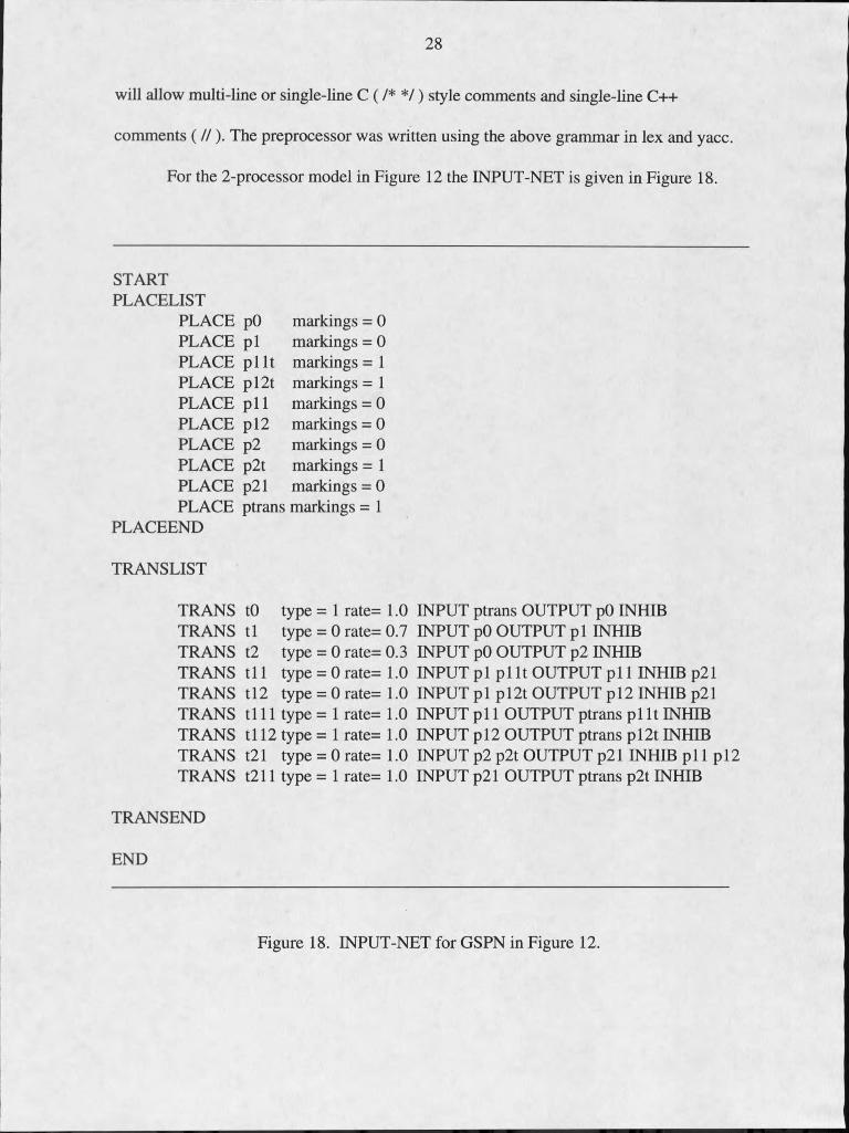
comments ( //) . The preprocessor was written using the above grammar in lex and yacc.
For the 2-processor model in Figure 12 the INPUT-NET is given in Figure 18.
STARTPLACELIST
PLACEPLACEPLACEPLACEPLACEPLACEPLACEPLACEPLACEPLACE
PLACEEND
pO markings = 0 p i markings = 0 p i It markings = I p!2t markings = I p i I markings = 0 p l2 markings = 0 p2 markings = 0 p2t markings = I p21 markings = 0 ptrans markings = I
TRANSLIST
TRANS tO type = I rate= 1.0 INPUT ptrans OUTPUT pO INHIB TRANS tl type = 0 rate= 0.7 INPUT pO OUTPUT p i INHIB TRANS t2 type = 0 rate= 0.3 INPUT pO OUTPUT p2 INHIB TRANS tl I type = 0 rate= 1.0 INPUT p i p i It OUTPUT p i I INHIB p21 TRANS t!2 type = 0 rate= 1.0 INPUT p i p!2t OUTPUT p!2 INHIB p21 TRANS t i l l type = I rate= 1.0 INPUT p i I OUTPUT ptrans p i It INHIB TRANS tl 12 type = I rate= 1.0 INPUT p!2 OUTPUT ptrans p!2t INHIB TRANS t2 1 type = 0 rate= 1.0 INPUT p2 p2t OUTPUT p21 INHIB p 11 p 12 TRANS t211 type = I rate= 1.0 INPUT p21 OUTPUT ptrans p2t INHIB
TRANSEND
END
Figure 18. INPUT-NET for GSPN in Figure 12.

29
The preprocessor will read the INPUT-NET, parse the contents of the net and
create the transition definitions needed for the kernel to operate on according to the
method in Figure 19.
• Insure that every place has an input and an output transition associated with it.
• Set the place definition structure with the initial marking.• Set the transition definition structure with the type of transition and the rate
values; every transition will have a firing function associated with it.• // Write the transition firing functions for all transitions
for all transitions dofor all places in the input list of the transition
for all transitions that are in the input list of the placeremove a token from the place and set these transitions as vanishing and remove them from queue,
endforfor all transitions that are in the inhib list of the place
disable the transition and remove from the queue, endfor
endforfor all places in the output list of the transition
for all transitions that are in the inhib list of the placeadd a token to the place and add the transition to the queue,
endforfor all transitions that are in the input list of the place
add transition to queue, endfor
endfor endfor
Figure 19. The preprocessor algorithm.
30
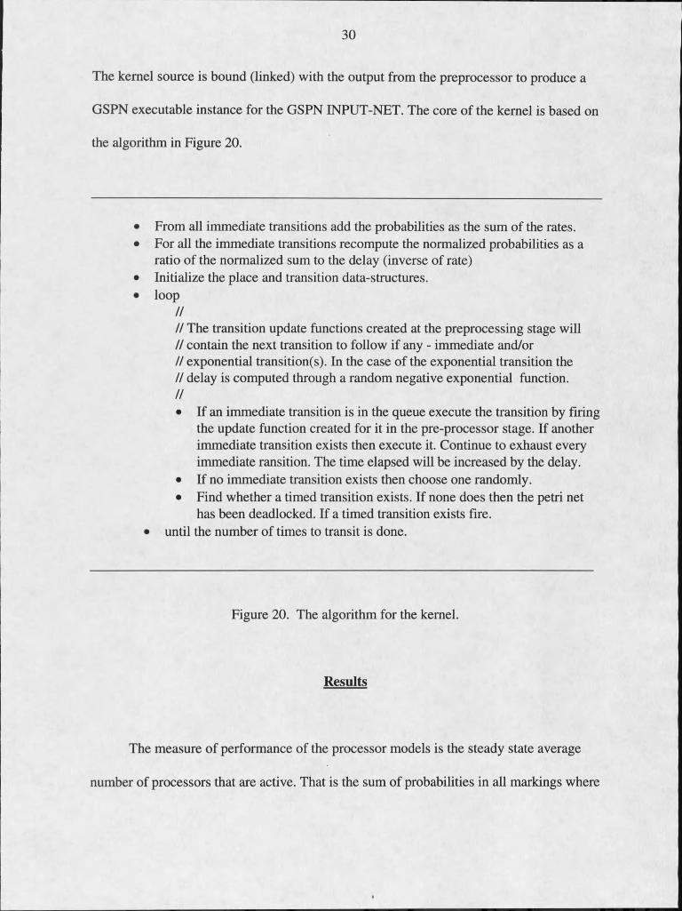
The kernel source is bound (linked) with the output from the preprocessor to produce a
GSPN executable instance for the GSPN INPUT-NET. The core of the kernel is based on
the algorithm in Figure 20.
• From all immediate transitions add the probabilities as the sum of the rates.• For all the immediate transitions recompute the normalized probabilities as a
ratio of the normalized sum to the delay (inverse of rate)• Initialize the place and transition data-structures.• loop
//// The transition update functions created at the preprocessing stage will // contain the next transition to follow if any - immediate and/or // exponential transition(s). In the case of the exponential transition the // delay is computed through a random negative exponential function.//• If an immediate transition is in the queue execute the transition by firing
the update function created for it in the pre-processor stage. If another immediate transition exists then execute it. Continue to exhaust every immediate ransition. The time elapsed will be increased by the delay.
• If no immediate transition exists then choose one randomly.• Find whether a timed transition exists. If none does then the petri net
has been deadlocked. If a timed transition exists fire.• until the number of times to transit is done.
Figure 20. The algorithm for the kernel.
Results
The measure of performance of the processor models is the steady state average
number of processors that are active. That is the sum of probabilities in all markings where

31
there are tokens in places p i and p2 in the 2-processor model and in all markings where
there are tokens in places p i, p2, and p3 in the 3-processor model. The load factor is
characterized as the ratio of a by p.
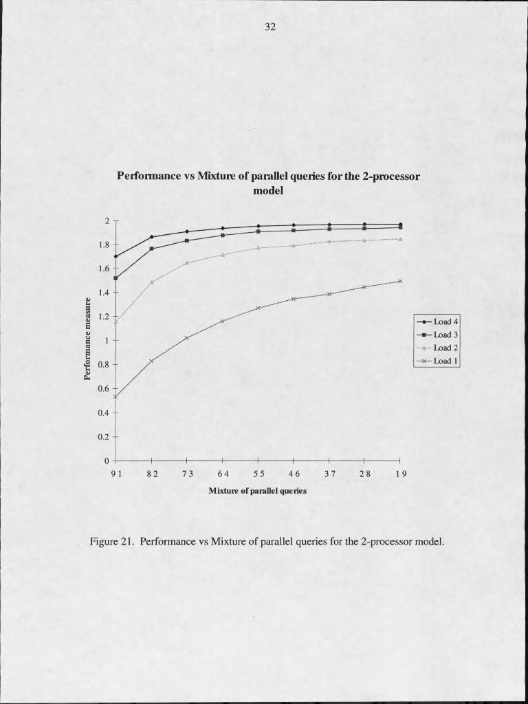
The Figures 21 and 22 are charts that show performance measure with respect to
the mixture of the job stream and the load factor for the 2-processor model. In Figure 21
we can see the improved performance as the job mix goes from 90% !-processor queries
and 10% 2-processor queries to the opposite side of the spectrum which is 10% 1-
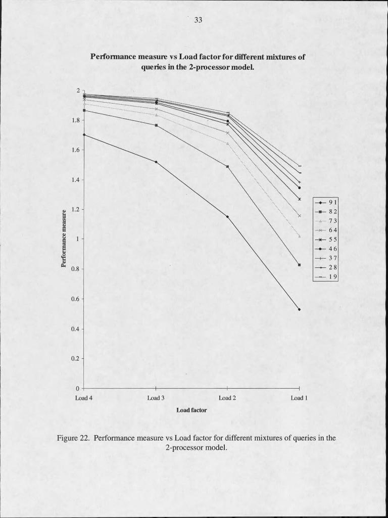
processor queries and 90% 2-processor queries. In Figure 22 as the load increases on the
two systems we can observe the uniform degradation of the system.
The results for the 2-processor model clearly suggests that as the load increases
the performance of the system will degrade irrespective of the job mix. Also, the larger the
fraction of the 2-processor queries, the better the performance. It is important to realize
that one processor queries do contend for the same processor in this model.
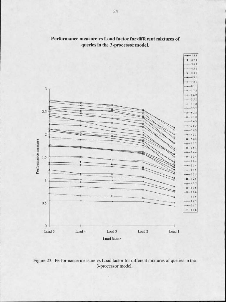
Figure 23 is the chart that shows the effect on performance measure as the mixture
of the different queries presented to the system is altered in the 3-processor model. Again,
it is evident that the larger the proportion of 3-, 2-, and !-processor requests, in that
order, the greater the performance of the system. The effect of the load factor on
performance is again uniform degradation as the load increases. It was always assumed in
the measurement that at no time will there be a lack of the I- or 2-processor requests in
the system. If that was not the case and the only job requests were 3-processor requests,
the performance measure will be close to three.
32
Performance vs Mixture of parallel queries for the 2-processormodel
1.8 -
1.4 -
1.2
0.8
0.6 - -
0.4 -
0.2 - -
Mixture of parallel queries
—♦—Load 4
- • —Load 3..*- Load 2
—x— Load I
Figure 21. Performance vs Mixture of parallel queries for the 2-processor model.
33
Performance measure vs Load factor for different mixtures of queries in the 2-processor model.
Load factor
9 I 8 2 7 3
— 6 4 —*— 5 5 — 4 6
- i — 3 7 — — 2 8
— I 9
Figure 22. Performance measure vs Load factor for different mixtures of queries in the2-processor model.
Per
form
anc
34
Performance measure vs Load factor for different mixtures of queries in the 3-processor model.
3 T
— I 8 I
- * — 2 7 I
A 3 6 1
......... 4 5 1
— 5 4 I
- * — 6 3 I
—I— 7 2 I
— .— 8 I I
.......... 17 2
* ...2 6 2
* - 3 5 2
4 4 2
—X— 5 3 2
— X— 6 2 2
— 7 I 2
16 3
....«—•— 2 5 3
—w— 3 4 3
4 3 3
5 2 3
—A— 6 I 2
- 1 5 4
—*— 2 4 4
••••*....3 3 4
—H— 4 2 4
....■ 5 14
— I 4 5
—♦— 2 3 5
- * — 3 25
—A— 4 I 5
—X— 1 3 6
- X — 2 2 6
3 I 6
— I 2 7..... 2 17
------- 1 I 8
O - I - - - - - - - - - - - - - - - - - - - - - 1- - - - - - - - - - - - - - - - - - - - - 1- - - - - - - - - - - - - - - - - - - - - 1- - - - - - - - - - - - - - - - - - - - - 1Load 5 Load 4 Load 3 Load 2 Load I
Load factor
Figure 23. Performance measure vs Load factor for different mixtures of queries in the3-processor model.

35
Limitations of the current models and suggestions for future research
The current models are based on the First Come First Served approach. Most real
world solutions are of this approach. It is possible to change the scheduling of the requests
by a lookahead mechanism. For example, when a 2-processor request is first in the queue
and the next one is another 2-processor request, this lookahead method will search for the
next request to see if it is a !-processor request.
The current models are bulky and the number of places and transitions will
increase as the number of processors increase. The net needs to be redone every time a
processor is added to the system. A general purpose solution that will model the
processors as the number of tokens in a place in the initial marking of the net would be
desirable.
The models had a high degree of liveness and never experienced deadlock. It
would be desirable to modify the implementation to study these properties.
I
36
BIBLIOGRAPHY
1. M. A. Holliday and M. K. Vernon. A generalized timed Petri net model for performance analysis. DEEE Transactions on Software Engineering, Vol. SE-13, No. 12, pages 1297-1310, Dec 1987. IEEE Computer Society Press.
2. M. D. P. Leland and W. D. Roome. The Silicon Database Machine. In Proceedings 4th International Workshop on Database Machines, pages 169-189, March 1985.
3. M. A. Marsan, G. Conte, and G. Balbo. A Class o f Generalized Stochastic Petri Nets fo r the Performance Evaluation o f Multiprocessor Systems. ACM Transactions on Computer Systems, Vol. 2, No. 2, pages 93-122, May 1984.
4. M. A. Marsan. Stochastic Petri Nets: An Elementary Introduction. In Gregorz Rozenberg, editor. Advances in Petri Nets 1989, pages 1-29. Springer-Verlag, 1989.
5. M. A. Marsan, G. Balbo, and G. Conte. Generalized Stochastic Petri nets revisited: Random switches and priorities. ACM Transaction on Computer Systems. Vol 2 No. I, pages 93-122, May 1984.
6. M. A. Marsan, G. Balbo, A. Bobbio, G. Chiola, G. Conte, and A. Cumani. The Effect o f Execution Policies on the Semantics and Analysis o f Stochastic Petri Nets. IEEE Transactions on Software Engineering. Vol. 15 No. 7, pages 832-846, July 1989
7. M. A. Marsan, G. Balbo, A. Bobbio, G. Chiola, G. Conte, and A. Cumani.. On Petri nets with Stochastic Timing. In Proceedings of the 1985 Workshop on Timed Petri Nets, pages 80-87, Torino, Italy, July 1985. DEEE Computer Society Press.
8. M. K. Molloy. Performance analysis using stochastic Petri nets. DEEE Transactions on Computers, Vol. C-31, No. 9, pages 913-917, 1982.
9. M. K. Molloy. On the integration of delay and throughput measures in distributed processing models. Ph.D. dissertation, University of California, Los Angeles, 1981.
10. S. Natkin. Les reseaux de Petri Stochastiques et Ieur application a V evaluation des systems informatiques. Ph.D. dissertation, CNAM-PARIS, June 1980.
11. M. T. Ozsu and P. Valduriez. Principles o f Distributed Database Systems. Englewood Cliffs, Prentice-Hall, 1991.

37
12.1. L. Peterson. Petri Net Theory and the Modeling o f Systems. Englewood Cliffs, Prentice Hall, 1981.
13. C. A. Petri. Communication with Automata. Ph.D. dissertation, Tech. Rep. RADC- TR-65-377, Rome Air Development Center, Rome, NY, 1966.
14. C. V. Ramamoorthy and G. S. Ho. Performance evaluation o f asynchronous concurrent systems using Petri nets. IEEE Transactions on Software Engineering, Vol SE-6, No. 5, pages 440-449, Sep 1980.

1762 1025 Ii1S f