Performance Analysis of Noise Cancellation in Speech ...ijmo.org/papers/206-S4051.pdf · adaptive noise cancellation. In real time signal processing, where the computational power

Abstract—In this paper the eminence of the Fast Transversal

Least Mean Squares (FT-LMS) algorithm over LMS and RLS

algorithms is provided. This algorithm is designed to provide

similar performance to the standard LMS algorithm while

reducing the computation order. Finite precision effects are also

briefly discussed. Simulations are performed with these

algorithms to compare both the computational burden as well

as the performance for adaptive noise cancellation. Simulations

show that FT-LMS offers comparable performance with

respect to the standard RLS and LMS in addition to a large

reduction in computation time for higher order filters.

Index Terms—Adaptive filters, LMS, RLS, FT-LMS.

I. INTRODUCTION

Adaptive noise cancellation is the best possible solution

for noise removal in a wide range of fields. A desired signal

which is accidentally corrupted by some unwanted noise can

often be recovered by an adaptive noise canceller using the

least mean squares (LMS) algorithm. But the disadvantage in

using LMS algorithm is its excess mean-squared error, or

misadjustment which increases linearly with the desired

signal power. This leads to deteriorating performance when

the desired signal exhibits large power fluctuations and is a

grave problem in many speech processing applications. From

the standard point of performance, it is known [1] that the

Recursive Least- Squares (RLS) algorithm offers fast

convergence and good error performance in the presence of

any noise. This criterion makes this algorithm beneficial for

adaptive noise cancellation. In real time signal processing,

where the computational power is considered, and at present

as the computational power of devices increases, it is difficult

to use RLS algorithm. The RLS algorithm is difficult to

implement because of its computational complexity. The

computation time of the algorithm scales with O(2M ),

where M is the filter order. This makes the computation of

RLS in real-time nearly impossible especially when higher

filter lengths are used. In this paper we provide a better

alternative filter Fast transversal LMS (FT-LMS) filter. This

filter is designed in such a manner that it provides the least

squares solution to the given adaptive filtering problem

which scales the computation time to O(M),which makes this

feasible for real-time applications. The rest of the paper is

organized in the following manner. Section II provides an

overview of LMS algorithm. Section III briefs the RLS

algorithm. Section IV gives an overview about FT-LMS

Manuscript received August 23, 2012; revised September 30, 2012.

D. Hari Hara Santosh is with MVGR College of Engineering, India

(e-mail: [email protected]).

algorithm. Section V will provide simulation results of

FT-LMS, RLS and RLS filters and discusses about their

performance in reducing noise. Section VI will provide

conclusions on this work.

II. LMS ALGORITHM

Least mean squares (LMS) algorithms are one of the class

of adaptive filters used to produce a desired filter by finding

the filter coefficients which produce the least mean squares

of the error signal (difference between the desired and the

actual signal). The Least Mean Square (LMS) algorithm is

an adaptive algorithm, which uses a gradient-based method

of steepest decent [2]. LMS algorithm uses the estimates of

the gradient vector from the available data. LMS follows an

iterative procedure that makes successive corrections to the

weight vector which eventually leads to the minimum mean

square error

The LMS algorithm is a linear adaptive filtering algorithm,

which consists of two basic processes:

1) A filtering process, which

a) Computes the output of a linear filter in response to

an input signal and

b) Generates an estimation error by comparing this

output with a desired response

2) An adaptive process, which adjusts the parameters

of the filter in accordance with the estimation error

LMS algorithm is important because of its simplicity and

ease of computation and because it does not require off-line

gradient estimation or repetitions of data

A. LMS Algorithm Formulation: 1

0

( ) ( ) ( 1)N

i

y n w n x n

(1)

( ) ( ) ( )e n d n y n (2)

We assume that the signals involved are real valued the

LMS algorithm changes (adapts) the filter tap weights to

minimize the error e (n). When the process x (n) and d (n) are

jointly stationary, this algorithm converges to a set of

tap-weights which on average are equal to the Wiener-Hopf

solution

The conventional LMS algorithm is a stochastic

implementation of the steepest descent algorithm.

)]([ 2 neE by its instantaneous coarse estimate

)(2 ne

Substituting )(2 ne for ζ in the steepest descent

recursion, we obtain

2( 1) ( ) ( )W n W n e n (3)

Performance Analysis of Noise Cancellation in Speech

Signals Using LMS, FT-LMS and RLS Algorithms

D. Hari Hara Santosh, Member IACSIT, Samalla Aditya, K. Sarat Chandra, and P. Surya Prasad

International Journal of Modeling and Optimization, Vol. 2, No. 6, December 2012

667DOI: 10.7763/IJMO.2012.V2.206

where,

T

N nwnwnwnW )](.).........()([)( 110

T

nwww]........................[

110

Note that the i-th element of the gradient vector )(2 ne is

ii w

nene

w

e

)()(2

2

(4) 2 ( ) ( 1)e n x n

Then

)()(2)(2 nxnene

Finally we obtain

( 1) ( ) 2 ( ) ( )W n W n e n x n (5)

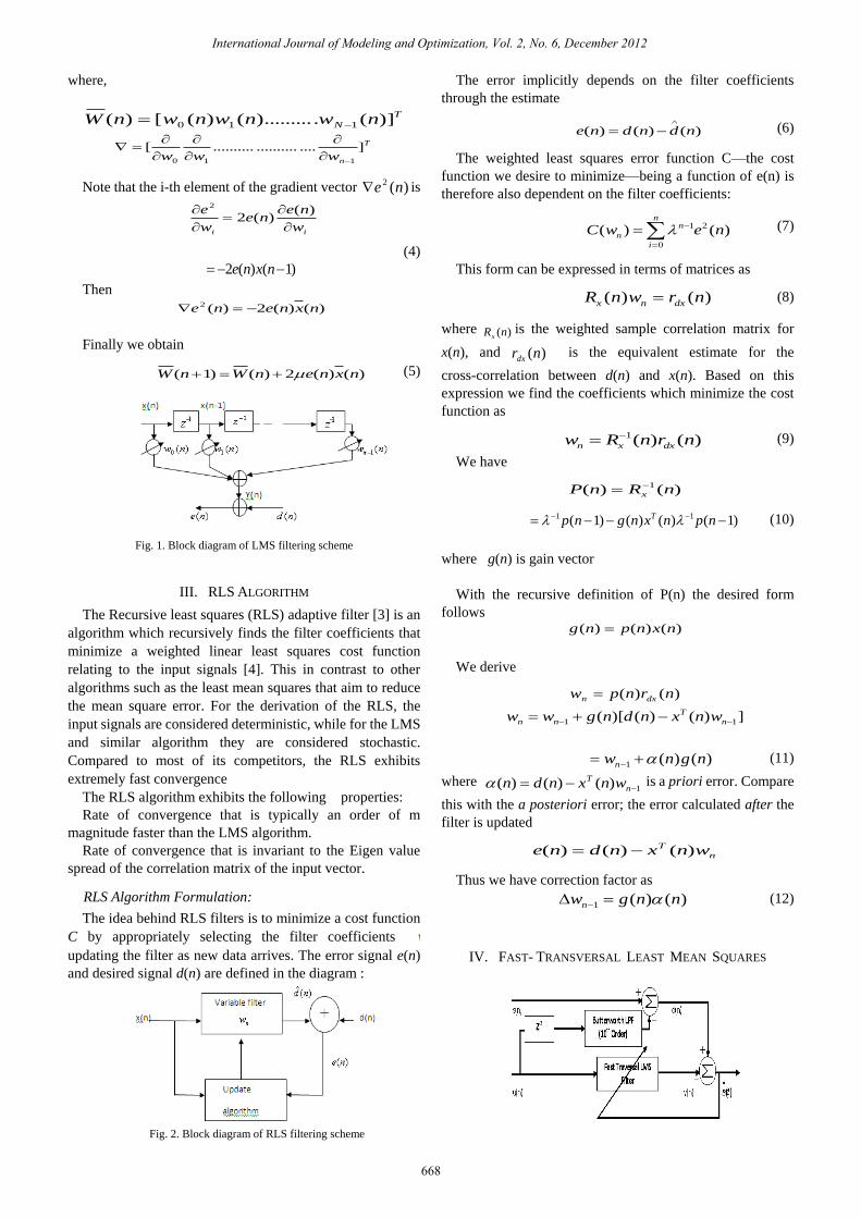
Fig. 1. Block diagram of LMS filtering scheme

III. RLS ALGORITHM

The Recursive least squares (RLS) adaptive filter [3] is an

algorithm which recursively finds the filter coefficients that

minimize a weighted linear least squares cost function

relating to the input signals [4]. This in contrast to other

algorithms such as the least mean squares that aim to reduce

the mean square error. For the derivation of the RLS, the

input signals are considered deterministic, while for the LMS

and similar algorithm they are considered stochastic.

Compared to most of its competitors, the RLS exhibits

extremely fast convergence

The RLS algorithm exhibits the following properties:

Rate of convergence that is typically an order of m

magnitude faster than the LMS algorithm.

Rate of convergence that is invariant to the Eigen value

spread of the correlation matrix of the input vector.

RLS Algorithm Formulation:

The idea behind RLS filters is to minimize a cost function

C by appropriately selecting the filter coefficients

updating the filter as new data arrives. The error signal e(n)

and desired signal d(n) are defined in the diagram :

Fig. 2. Block diagram of RLS filtering scheme

The error implicitly depends on the filter coefficients

through the estimate

( ) ( ) ( )e n d n d n

(6)

The weighted least squares error function C—the cost

function we desire to minimize—being a function of e(n) is

therefore also dependent on the filter coefficients:

1 2

0

( ) ( )n

n

n

i

C w e n

(7)

This form can be expressed in terms of matrices as

( ) ( )x n dxR n w r n (8)

where )(nRxis the weighted sample correlation matrix for

x(n), and )(nrdx is the equivalent estimate for the

cross-correlation between d(n) and x(n). Based on this

expression we find the coefficients which minimize the cost

function as

1( ) ( )n x dxw R n r n (9)

We have

)()( 1 nRnP x

1 1( 1) ( ) ( ) ( 1)Tp n g n x n p n (10)

where g(n) is gain vector

With the recursive definition of P(n) the desired form

follows )()()( nxnpng

We derive

)()( nrnpw dxn

])()()[( 11 n

T

nn wnxndngww

1 ( ) ( )nw n g n (11)

where 1)()()( n

T wnxndn is a priori error. Compare

this with the a posteriori error; the error calculated after the

filter is updated

n

T wnxndne )()()(

Thus we have correction factor as

1 ( ) ( )nw g n n (12)

IV. FAST- TRANSVERSAL LEAST MEAN SQUARES


668

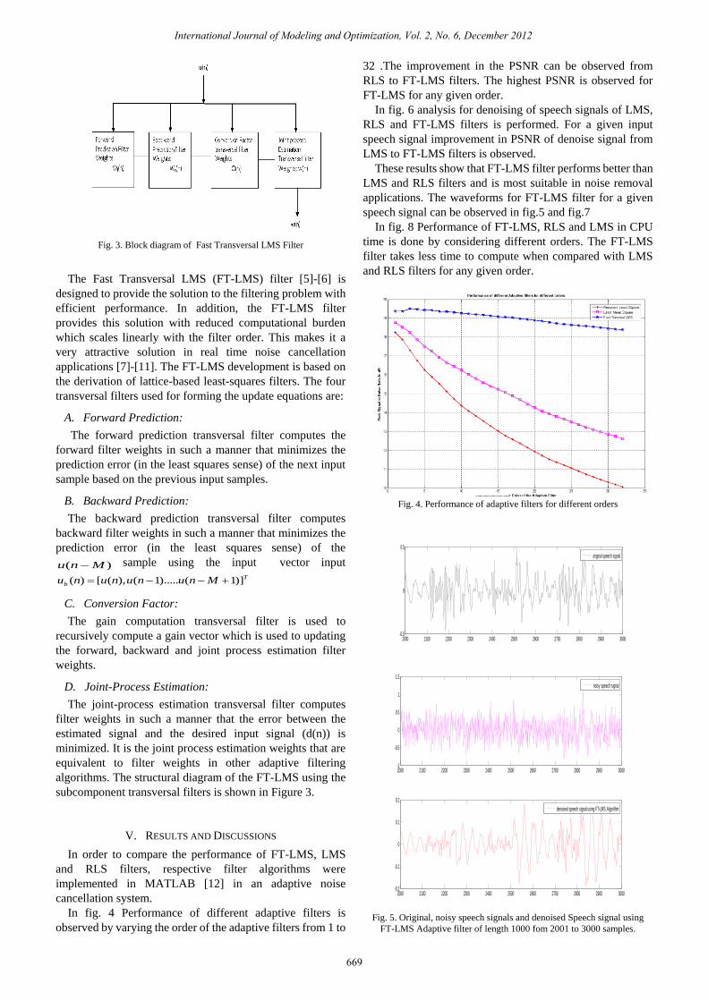
Fig. 3. Block diagram of Fast Transversal LMS Filter

The Fast Transversal LMS (FT-LMS) filter [5]-[6] is

designed to provide the solution to the filtering problem with

efficient performance. In addition, the FT-LMS filter

provides this solution with reduced computational burden

which scales linearly with the filter order. This makes it a

very attractive solution in real time noise cancellation

applications [7]-[11]. The FT-LMS development is based on

the derivation of lattice-based least-squares filters. The four

transversal filters used for forming the update equations are:

A. Forward Prediction:

The forward prediction transversal filter computes the

forward filter weights in such a manner that minimizes the

prediction error (in the least squares sense) of the next input

sample based on the previous input samples.

B. Backward Prediction:

The backward prediction transversal filter computes

backward filter weights in such a manner that minimizes the

prediction error (in the least squares sense) of the

)( Mnu sample using the input vector input T

b Mnunununu )]1().....1(),([)(

C. Conversion Factor:

The gain computation transversal filter is used to

recursively compute a gain vector which is used to updating

the forward, backward and joint process estimation filter

weights.

D. Joint-Process Estimation:

The joint-process estimation transversal filter computes

filter weights in such a manner that the error between the

estimated signal and the desired input signal (d(n)) is

minimized. It is the joint process estimation weights that are

equivalent to filter weights in other adaptive filtering

algorithms. The structural diagram of the FT-LMS using the

subcomponent transversal filters is shown in Figure 3.

V. RESULTS AND DISCUSSIONS

In order to compare the performance of FT-LMS, LMS

and RLS filters, respective filter algorithms were

implemented in MATLAB [12] in an adaptive noise

cancellation system.

In fig. 4 Performance of different adaptive filters is

observed by varying the order of the adaptive filters from 1 to

32 .The improvement in the PSNR can be observed from

RLS to FT-LMS filters. The highest PSNR is observed for

FT-LMS for any given order.

In fig. 6 analysis for denoising of speech signals of LMS,

RLS and FT-LMS filters is performed. For a given input

speech signal improvement in PSNR of denoise signal from

LMS to FT-LMS filters is observed.

These results show that FT-LMS filter performs better than

LMS and RLS filters and is most suitable in noise removal

applications. The waveforms for FT-LMS filter for a given

speech signal can be observed in fig.5 and fig.7

In fig. 8 Performance of FT-LMS, RLS and LMS in CPU

time is done by considering different orders. The FT-LMS

filter takes less time to compute when compared with LMS

and RLS filters for any given order.

Fig. 4. Performance of adaptive filters for different orders

2000 2100 2200 2300 2400 2500 2600 2700 2800 2900 3000-0.5

0

0.5

2000 2100 2200 2300 2400 2500 2600 2700 2800 2900 3000-0.2

-0.1

0

0.1

0.2

2000 2100 2200 2300 2400 2500 2600 2700 2800 2900 3000-1

-0.5

0

0.5

1

1.5

original speech signal

noisy speech signal

denoised speech signal using FT-LMS Algorithm

2000 2100 2200 2300 2400 2500 2600 2700 2800 2900 3000-0.5

0

0.5

2000 2100 2200 2300 2400 2500 2600 2700 2800 2900 3000-0.2

-0.1

0

0.1

0.2

2000 2100 2200 2300 2400 2500 2600 2700 2800 2900 3000-1

-0.5

0

0.5

1

1.5


noisy speech signal


Fig. 5. Original, noisy speech signals and denoised Speech signal using

FT-LMS Adaptive filter of length 1000 fom 2001 to 3000 samples.


669

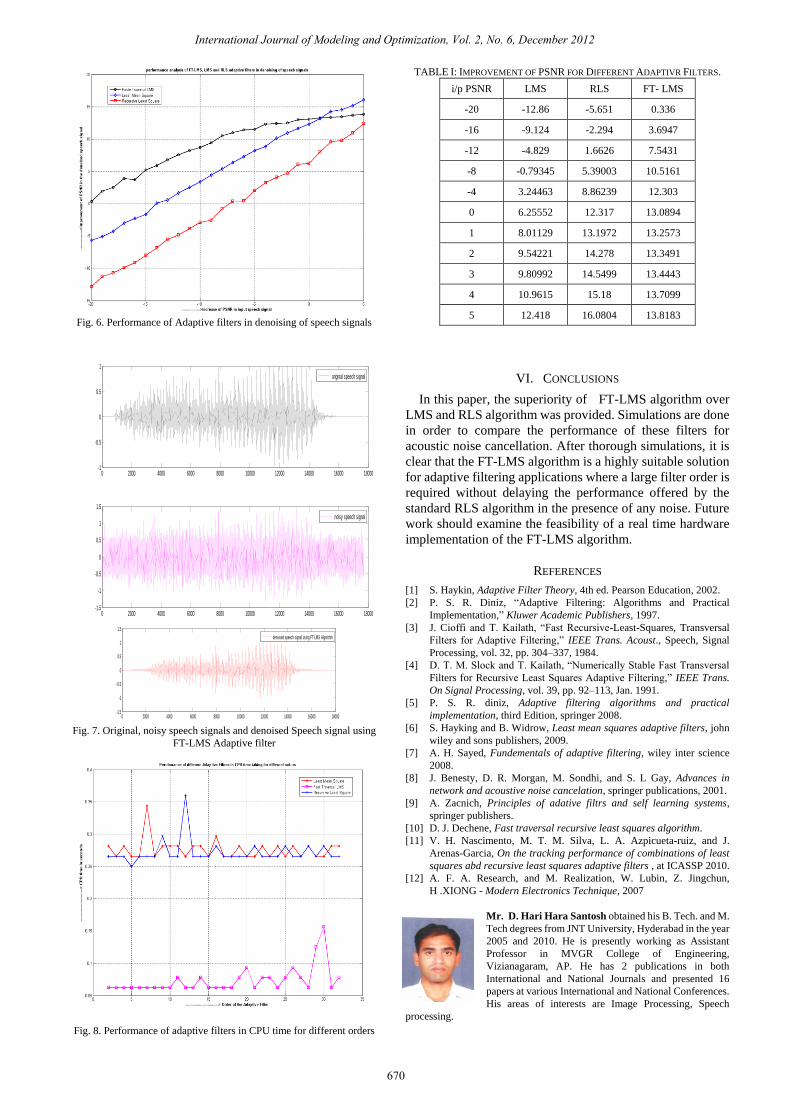
Fig. 6. Performance of Adaptive filters in denoising of speech signals

0 2000 4000 6000 8000 10000 12000 14000 16000 18000-1

-0.5

0

0.5

1

0 2000 4000 6000 8000 10000 12000 14000 16000 18000-1.5

-1

-0.5

0

0.5

1

1.5

0 2000 4000 6000 8000 10000 12000 14000 16000 18000-1.5

-1

-0.5

0

0.5

1

1.5


noisy speech signal


0 2000 4000 6000 8000 10000 12000 14000 16000 18000-1

-0.5

0

0.5

1

0 2000 4000 6000 8000 10000 12000 14000 16000 18000-1.5

-1

-0.5

0

0.5

1

1.5

0 2000 4000 6000 8000 10000 12000 14000 16000 18000-1.5

-1

-0.5

0

0.5

1

1.5


noisy speech signal


Fig. 7. Original, noisy speech signals and denoised Speech signal using

FT-LMS Adaptive filter

Fig. 8. Performance of adaptive filters in CPU time for different orders

TABLE I: IMPROVEMENT OF PSNR FOR DIFFERENT ADAPTIVR FILTERS.

i/p PSNR LMS RLS FT- LMS

-20 -12.86 -5.651 0.336

-16 -9.124 -2.294 3.6947

-12 -4.829 1.6626 7.5431

-8 -0.79345 5.39003 10.5161

-4 3.24463 8.86239 12.303

0 6.25552 12.317 13.0894

1 8.01129 13.1972 13.2573

2 9.54221 14.278 13.3491

3 9.80992 14.5499 13.4443

4 10.9615 15.18 13.7099

5 12.418 16.0804 13.8183

VI. CONCLUSIONS

In this paper, the superiority of FT-LMS algorithm over

LMS and RLS algorithm was provided. Simulations are done

in order to compare the performance of these filters for

acoustic noise cancellation. After thorough simulations, it is

clear that the FT-LMS algorithm is a highly suitable solution

for adaptive filtering applications where a large filter order is

required without delaying the performance offered by the

standard RLS algorithm in the presence of any noise. Future

work should examine the feasibility of a real time hardware

implementation of the FT-LMS algorithm.

REFERENCES

[1] S. Haykin, Adaptive Filter Theory, 4th ed. Pearson Education, 2002.

[2] P. S. R. Diniz, ―Adaptive Filtering: Algorithms and Practical

Implementation,‖ Kluwer Academic Publishers, 1997.

[3] J. Cioffi and T. Kailath, ―Fast Recursive-Least-Squares, Transversal

Filters for Adaptive Filtering,‖ IEEE Trans. Acoust., Speech, Signal

Processing, vol. 32, pp. 304–337, 1984.

[4] D. T. M. Slock and T. Kailath, ―Numerically Stable Fast Transversal

Filters for Recursive Least Squares Adaptive Filtering,‖ IEEE Trans.

On Signal Processing, vol. 39, pp. 92–113, Jan. 1991.

[5] P. S. R. diniz, Adaptive filtering algorithms and practical

implementation, third Edition, springer 2008.

[6] S. Hayking and B. Widrow, Least mean squares adaptive filters, john

wiley and sons publishers, 2009.

[7] A. H. Sayed, Fundementals of adaptive filtering, wiley inter science

2008.

[8] J. Benesty, D. R. Morgan, M. Sondhi, and S. L Gay, Advances in

network and acoustive noise cancelation, springer publications, 2001.

[9] A. Zacnich, Principles of adative filtrs and self learning systems,

springer publishers.

[10] D. J. Dechene, Fast traversal recursive least squares algorithm.

[11] V. H. Nascimento, M. T. M. Silva, L. A. Azpicueta-ruiz, and J.

Arenas-Garcia, On the tracking performance of combinations of least

squares abd recursive least squares adaptive filters , at ICASSP 2010.

[12] A. F. A. Research, and M. Realization, W. Lubin, Z. Jingchun,

H .XIONG - Modern Electronics Technique, 2007

Mr. D. Hari Hara Santosh obtained his B. Tech. and M.

Tech degrees from JNT University, Hyderabad in the year

2005 and 2010. He is presently working as Assistant

Professor in MVGR College of Engineering,

Vizianagaram, AP. He has 2 publications in both

International and National Journals and presented 16

papers at various International and National Conferences.

His areas of interests are Image Processing, Speech

processing.


670

Mr. Samalla Aitya completed his B. Tech. from MVGR

College of Engg., JNT University, Kakinada. He has

presented many papers at various student symposiums on

latest technologies. His areas of interests are Image

Processing, Speech processing.

Mr. K. Sarath Chandra completed his B. Tech. from

MVGR College of Engg., JNT University, Kakinada.

He has presented many papers at various student

symposiums on latest technologies. His areas of

interests are Image Processing, Speech processing.

Mr. P. Surya Prasad obtained his B. Tech. and M. Tech

degrees from JNT University, Kakinada and IIT Delhi in

the year 1998 and 2001. He is presently working as

Associate Professor in MVGR College of Engineering,

Vizianagaram, AP. He has 2 publications in both

International and National Journals and presented 14

papers at various International and National Conferences.

His areas of interests are Image Processing, Speech

processing.


671

Documents

Performance Analysis of Noise Cancellation in Speech ...ijmo.org/papers/206-S4051.pdf · adaptive noise cancellation. In real time signal processing, where the computational power