Performance Comparison of Rock Detection Algorithmsfor Autonomous Planetary Geology

David R. Thompson1 and Rebecca Castano2

1The Robotics Institute 2 Jet Propulsion LaboratoryCarnegie Mellon University California Institute of Technology

Pittsburgh, PA 15206 Pasadena, CA 91109(412) 628-7413 (818) 393-3544drt@ri.cmu.edu Rebecca.Castano@jpl.nasa.gov

Abstract—Detecting rocks in images is a valuable capabilityfor autonomous planetary science. Rock detection facilitatesselective data collection and return. It also assists with imageanalysis on Earth. This work reviews seven rock detectionalgorithms from the autonomous science literature. We eval-uate each algorithm with respect to several autonomous ge-ology applications. Tests show the algorithms’ performanceon Mars Exploration Rover imagery, terrestrial images fromanalog environments, and synthetic images from a Mars ter-rain simulator. This provides insight into the detectors’ per-formance under different imaging conditions.

TABLE OF CONTENTS

1 INTRODUCTION . . . . . . . . . . . . . . . . . . . . . . . . . . . . . . . 12 IMAGE DATASETS . . . . . . . . . . . . . . . . . . . . . . . . . . . . . 13 TESTED ALGORITHMS . . . . . . . . . . . . . . . . . . . . . . . . 24 PERFORMANCE EVALUATION . . . . . . . . . . . . . . . . . . 45 EXPERIMENTAL RESULTS . . . . . . . . . . . . . . . . . . . . . 56 DISCUSSION . . . . . . . . . . . . . . . . . . . . . . . . . . . . . . . . . . . 7

1. INTRODUCTION

Detecting rocks in images is a valuable capability for au-tonomous planetary science. Rocks are pristine targets forcompositional analysis with spectrometers. Their shape, size,and texture hold a wealth of geologic information. Com-puting the locations and distributions of rocks facilitates au-tonomous rover functions like adaptive target selection [4],selective image return [2], and autonomous site characteriza-tion [12]. Moreover, automatic rock detection can assist off-board data analysis. Rock size and shape distributions carryimportant geologic cues, but the manual analysis required tocharacterize these distributions is extremely time intensive.Currently scientists evaluate these statistics over very limitedregions. Accurate rock detection would generate these richdata products quickly and cheaply.

Unfortunately rock detection is a difficult pattern recognitionproblem. Rocks exhibit diverse morphologies, colors andtextures. They are often covered in dust, grouped into self-

0-7803-8870-4/05/ $ 20.00/c©2007 IEEE

IEEEAC paper # 1251

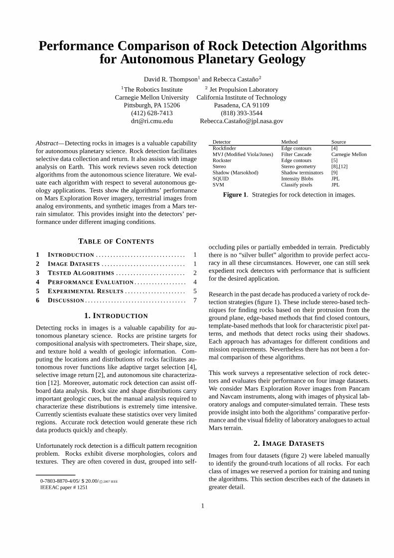
Detector Method SourceRockfinder Edge contours [4]MVJ (Modified Viola/Jones) Filter Cascade Carnegie MellonRockster Edge contours [5]Stereo Stereo geometry [8],[12]Shadow (Marsokhod) Shadow terminators [9]SQUID Intensity Blobs JPLSVM Classify pixels JPL

Figure 1. Strategies for rock detection in images.

occluding piles or partially embedded in terrain. Predictablythere is no “silver bullet” algorithm to provide perfect accu-racy in all these circumstances. However, one can still seekexpedient rock detectors with performance that is sufficientfor the desired application.

Research in the past decade has produced a variety of rock de-tection strategies (figure 1). These include stereo-based tech-niques for finding rocks based on their protrusion from theground plane, edge-based methods that find closed contours,template-based methods that look for characteristic pixelpat-terns, and methods that detect rocks using their shadows.Each approach has advantages for different conditions andmission requirements. Nevertheless there has not been a for-mal comparison of these algorithms.

This work surveys a representative selection of rock detec-tors and evaluates their performance on four image datasets.We consider Mars Exploration Rover images from Pancamand Navcam instruments, along with images of physical lab-oratory analogs and computer-simulated terrain. These testsprovide insight into both the algorithms’ comparative perfor-mance and the visual fidelity of laboratory analogues to actualMars terrain.

2. IMAGE DATASETS

Images from four datasets (figure 2) were labeled manuallyto identify the ground-truth locations of all rocks. For eachclass of images we reserved a portion for training and tuningthe algorithms. This section describes each of the datasetsingreater detail.

1

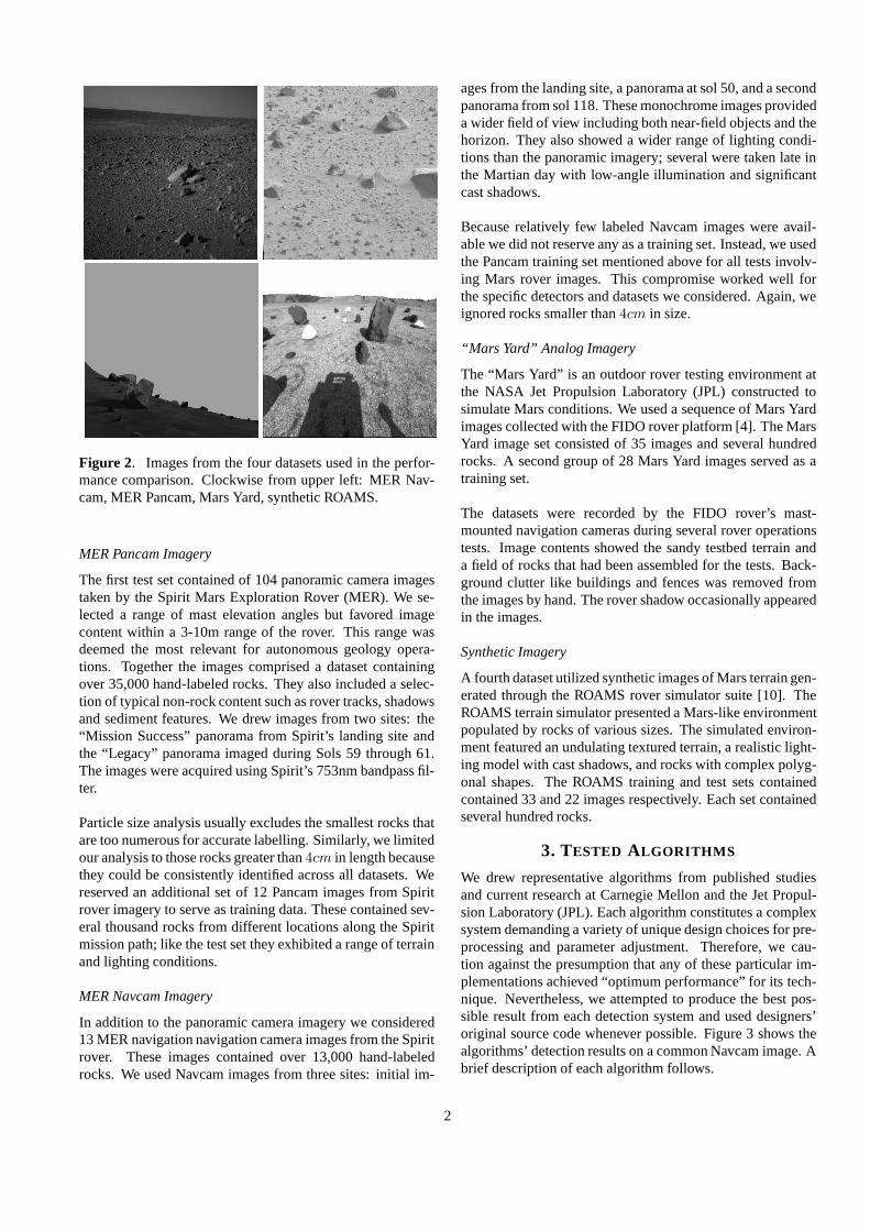
Figure 2. Images from the four datasets used in the perfor-mance comparison. Clockwise from upper left: MER Nav-cam, MER Pancam, Mars Yard, synthetic ROAMS.

MER Pancam Imagery

The first test set contained of 104 panoramic camera imagestaken by the Spirit Mars Exploration Rover (MER). We se-lected a range of mast elevation angles but favored imagecontent within a 3-10m range of the rover. This range wasdeemed the most relevant for autonomous geology opera-tions. Together the images comprised a dataset containingover 35,000 hand-labeled rocks. They also included a selec-tion of typical non-rock content such as rover tracks, shadowsand sediment features. We drew images from two sites: the“Mission Success” panorama from Spirit’s landing site andthe “Legacy” panorama imaged during Sols 59 through 61.The images were acquired using Spirit’s 753nm bandpass fil-ter.

Particle size analysis usually excludes the smallest rocksthatare too numerous for accurate labelling. Similarly, we limitedour analysis to those rocks greater than4cm in length becausethey could be consistently identified across all datasets. Wereserved an additional set of 12 Pancam images from Spiritrover imagery to serve as training data. These contained sev-eral thousand rocks from different locations along the Spiritmission path; like the test set they exhibited a range of terrainand lighting conditions.

MER Navcam Imagery

In addition to the panoramic camera imagery we considered13 MER navigation navigation camera images from the Spiritrover. These images contained over 13,000 hand-labeledrocks. We used Navcam images from three sites: initial im-

ages from the landing site, a panorama at sol 50, and a secondpanorama from sol 118. These monochrome images provideda wider field of view including both near-field objects and thehorizon. They also showed a wider range of lighting condi-tions than the panoramic imagery; several were taken late inthe Martian day with low-angle illumination and significantcast shadows.

Because relatively few labeled Navcam images were avail-able we did not reserve any as a training set. Instead, we usedthe Pancam training set mentioned above for all tests involv-ing Mars rover images. This compromise worked well forthe specific detectors and datasets we considered. Again, weignored rocks smaller than4cm in size.

“Mars Yard” Analog Imagery

The “Mars Yard” is an outdoor rover testing environment atthe NASA Jet Propulsion Laboratory (JPL) constructed tosimulate Mars conditions. We used a sequence of Mars Yardimages collected with the FIDO rover platform [4]. The MarsYard image set consisted of 35 images and several hundredrocks. A second group of 28 Mars Yard images served as atraining set.

The datasets were recorded by the FIDO rover’s mast-mounted navigation cameras during several rover operationstests. Image contents showed the sandy testbed terrain anda field of rocks that had been assembled for the tests. Back-ground clutter like buildings and fences was removed fromthe images by hand. The rover shadow occasionally appearedin the images.

Synthetic Imagery

A fourth dataset utilized synthetic images of Mars terrain gen-erated through the ROAMS rover simulator suite [10]. TheROAMS terrain simulator presented a Mars-like environmentpopulated by rocks of various sizes. The simulated environ-ment featured an undulating textured terrain, a realistic light-ing model with cast shadows, and rocks with complex polyg-onal shapes. The ROAMS training and test sets containedcontained 33 and 22 images respectively. Each set containedseveral hundred rocks.

3. TESTED ALGORITHMS

We drew representative algorithms from published studiesand current research at Carnegie Mellon and the Jet Propul-sion Laboratory (JPL). Each algorithm constitutes a complexsystem demanding a variety of unique design choices for pre-processing and parameter adjustment. Therefore, we cau-tion against the presumption that any of these particular im-plementations achieved “optimum performance” for its tech-nique. Nevertheless, we attempted to produce the best pos-sible result from each detection system and used designers’original source code whenever possible. Figure 3 shows thealgorithms’ detection results on a common Navcam image. Abrief description of each algorithm follows.

2

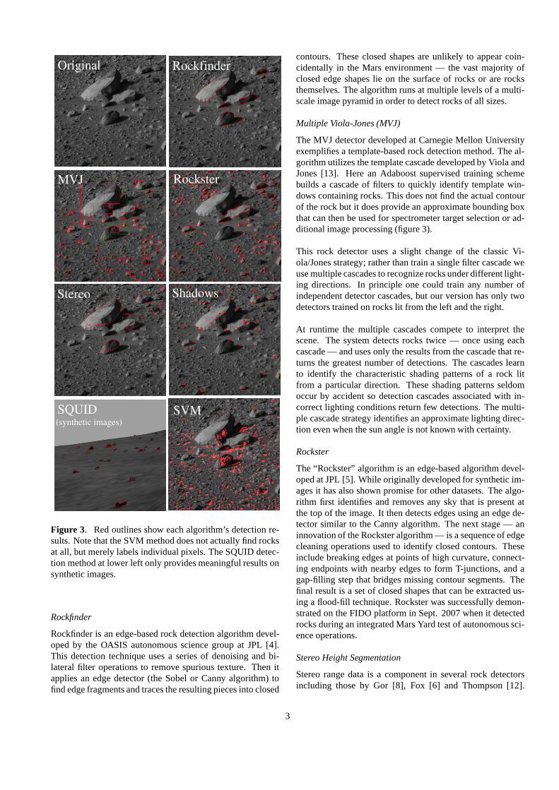
Figure 3. Red outlines show each algorithm’s detection re-sults. Note that the SVM method does not actually find rocksat all, but merely labels individual pixels. The SQUID detec-tion method at lower left only provides meaningful results onsynthetic images.

Rockfinder

Rockfinder is an edge-based rock detection algorithm devel-oped by the OASIS autonomous science group at JPL [4].This detection technique uses a series of denoising and bi-lateral filter operations to remove spurious texture. Then itapplies an edge detector (the Sobel or Canny algorithm) tofind edge fragments and traces the resulting pieces into closed

contours. These closed shapes are unlikely to appear coin-cidentally in the Mars environment — the vast majority ofclosed edge shapes lie on the surface of rocks or are rocksthemselves. The algorithm runs at multiple levels of a multi-scale image pyramid in order to detect rocks of all sizes.

Multiple Viola-Jones (MVJ)

The MVJ detector developed at Carnegie Mellon Universityexemplifies a template-based rock detection method. The al-gorithm utilizes the template cascade developed by Viola andJones [13]. Here an Adaboost supervised training schemebuilds a cascade of filters to quickly identify template win-dows containing rocks. This does not find the actual contourof the rock but it does provide an approximate bounding boxthat can then be used for spectrometer target selection or ad-ditional image processing (figure 3).

This rock detector uses a slight change of the classic Vi-ola/Jones strategy; rather than train a single filter cascade weuse multiple cascades to recognize rocks under different light-ing directions. In principle one could train any number ofindependent detector cascades, but our version has only twodetectors trained on rocks lit from the left and the right.

At runtime the multiple cascades compete to interpret thescene. The system detects rocks twice — once using eachcascade — and uses only the results from the cascade that re-turns the greatest number of detections. The cascades learnto identify the characteristic shading patterns of a rock litfrom a particular direction. These shading patterns seldomoccur by accident so detection cascades associated with in-correct lighting conditions return few detections. The multi-ple cascade strategy identifies an approximate lighting direc-tion even when the sun angle is not known with certainty.

Rockster

The “Rockster” algorithm is an edge-based algorithm devel-oped at JPL [5]. While originally developed for synthetic im-ages it has also shown promise for other datasets. The algo-rithm first identifies and removes any sky that is present atthe top of the image. It then detects edges using an edge de-tector similar to the Canny algorithm. The next stage — aninnovation of the Rockster algorithm — is a sequence of edgecleaning operations used to identify closed contours. Theseinclude breaking edges at points of high curvature, connect-ing endpoints with nearby edges to form T-junctions, and agap-filling step that bridges missing contour segments. Thefinal result is a set of closed shapes that can be extracted us-ing a flood-fill technique. Rockster was successfully demon-strated on the FIDO platform in Sept. 2007 when it detectedrocks during an integrated Mars Yard test of autonomous sci-ence operations.

Stereo Height Segmentation

Stereo range data is a component in several rock detectorsincluding those by Gor [8], Fox [6] and Thompson [12].

3

These algorithms follow a common formula. They fit a pla-nar ground model to the terrain using least-squares regressionor RANSAC [7]. Then they find each pixel’s distance to theplane in order to create a height map. A segmentation of thisheight map identifies image regions that protrude above thesurface.

We implemented a version of stereo hight segmentation forthis work. Our version follows Gor’s strategy of detectingheight-map discontinuities that indicate the tops of rocks.We apply a vertical derivative filter that responds stronglytothese discontinuities. After finding the topmost rock pixels,a region-growing operation grows the rock regions down to aminimum height. The result is a segmentation of the rocks inthe scene. Unlike the original Gor algorithm, we also applya high-pass filter to the initial hieghtmap. This removes low-frequency changes in height like terrain bumps to improveperformance when the ground is not perfectly planar.

Marsokhod Shadow Detector

We examine the rock detection algorithm used for image anal-ysis during the 1999 Marsokhod rover field tests [9]. Thismethod is one of the first examples of rock detection for au-tonomous science applications. It reduces the rock detectionproblem to one of finding shadows. Given a known sun an-gle, shadows suggest the location of rocks in the scene. TheMarsokhod detector utilizes a spherical lighting model to pre-dict the orientation of terminator lines (separating illuminatedfrom darkened sides of the rock). It uses an edge detectorto find candidate terminators, and selects appropriate candi-dates using edge orientations. While the result does not findthe contour outline of the rock, it does identify a point on therock’s surface that can be used as a target for spectroscopy.

SQUID

TheSmoothed Quick Uniform Intensity Detectoris a simplealgorithm developed for use on synthetic images. First a bilat-eral filtering algorithm removes terrain texture. Then a simpleintensity segmentation scheme identifies contiguous areasofconstant pixel intensity. In this manner it locates contiguousblobs of intensity; a size filter discounts large blobs as belong-ing to the sky or terrain. Any remaining blobs are presumedto be rocks.

SVM Pixel Classification

Finally we investigate an algorithm that classifies every imagepixel individually. These pixel classifications do not revealthe contours of each individual rock, but they can estimatethe fractional coverage of rocks in the image. The algorithmuses a support vector machine classifier to analyze local win-dows around each pixel. It characterizes each pixel using afeature vector constructed from local intensity values. TheSVM identified individual pixels that were most likely to lieon rocks.

4. PERFORMANCE EVALUATION

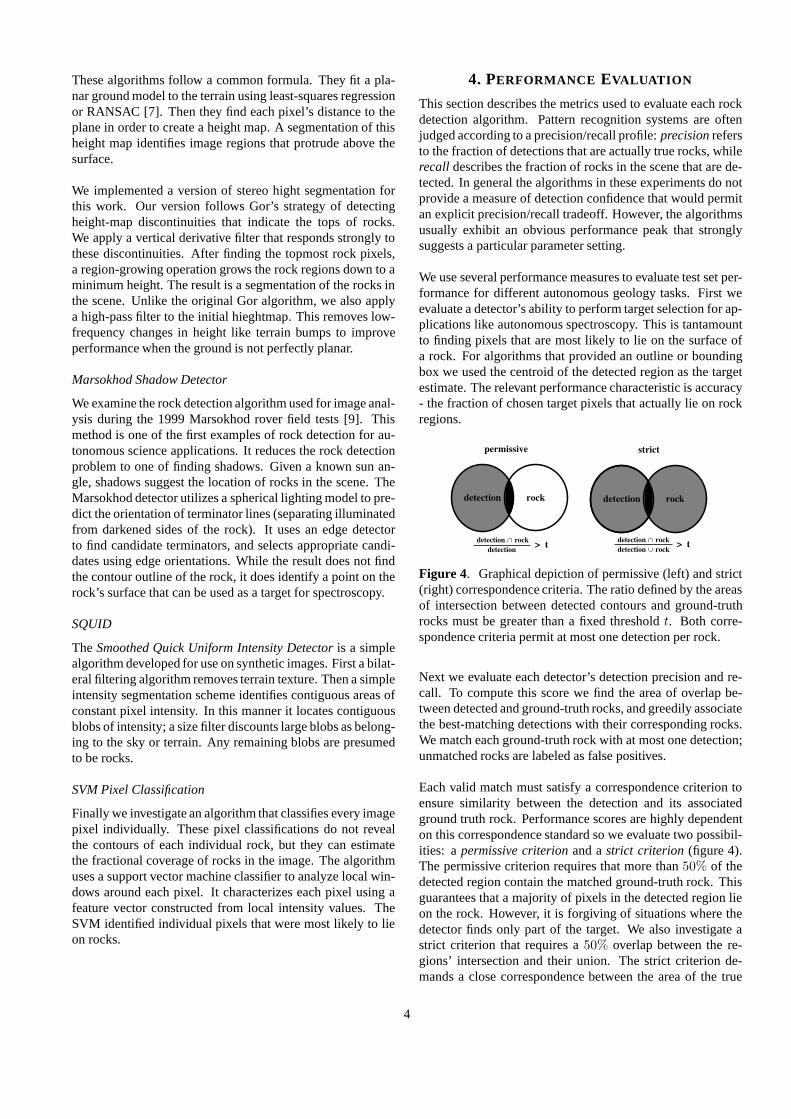
This section describes the metrics used to evaluate each rockdetection algorithm. Pattern recognition systems are oftenjudged according to a precision/recall profile:precisionrefersto the fraction of detections that are actually true rocks, whilerecall describes the fraction of rocks in the scene that are de-tected. In general the algorithms in these experiments do notprovide a measure of detection confidence that would permitan explicit precision/recall tradeoff. However, the algorithmsusually exhibit an obvious performance peak that stronglysuggests a particular parameter setting.

We use several performance measures to evaluate test set per-formance for different autonomous geology tasks. First weevaluate a detector’s ability to perform target selection for ap-plications like autonomous spectroscopy. This is tantamountto finding pixels that are most likely to lie on the surface ofa rock. For algorithms that provided an outline or boundingbox we used the centroid of the detected region as the targetestimate. The relevant performance characteristic is accuracy- the fraction of chosen target pixels that actually lie on rockregions.

Figure 4. Graphical depiction of permissive (left) and strict(right) correspondence criteria. The ratio defined by the areasof intersection between detected contours and ground-truthrocks must be greater than a fixed thresholdt. Both corre-spondence criteria permit at most one detection per rock.

Next we evaluate each detector’s detection precision and re-call. To compute this score we find the area of overlap be-tween detected and ground-truth rocks, and greedily associatethe best-matching detections with their corresponding rocks.We match each ground-truth rock with at most one detection;unmatched rocks are labeled as false positives.

Each valid match must satisfy a correspondence criterion toensure similarity between the detection and its associatedground truth rock. Performance scores are highly dependenton this correspondence standard so we evaluate two possibil-ities: apermissive criterionand astrict criterion (figure 4).The permissive criterion requires that more than50% of thedetected region contain the matched ground-truth rock. Thisguarantees that a majority of pixels in the detected region lieon the rock. However, it is forgiving of situations where thedetector finds only part of the target. We also investigate astrict criterion that requires a50% overlap between the re-gions’ intersection and their union. The strict criterion de-mands a close correspondence between the area of the true

4

rock and the detected region, so it better indicates the accu-racy of automatically-computed rock attributes like size orshape.

Finally we evaluate autonomous prediction of the fractionalarea of terrain covered by rocks. We count detected rockpixels individually and compare the resulting count to theground-truth fraction for each image. This standard does notrequire any correspondence between detected and actual rockpixels; it only concerns the total predicted number of rockpixels.

Rockfinder MVJ Rockster Stereo Shadows0.0

0.2

0.4

0.6

0.8

1.0

pre

cis

ion

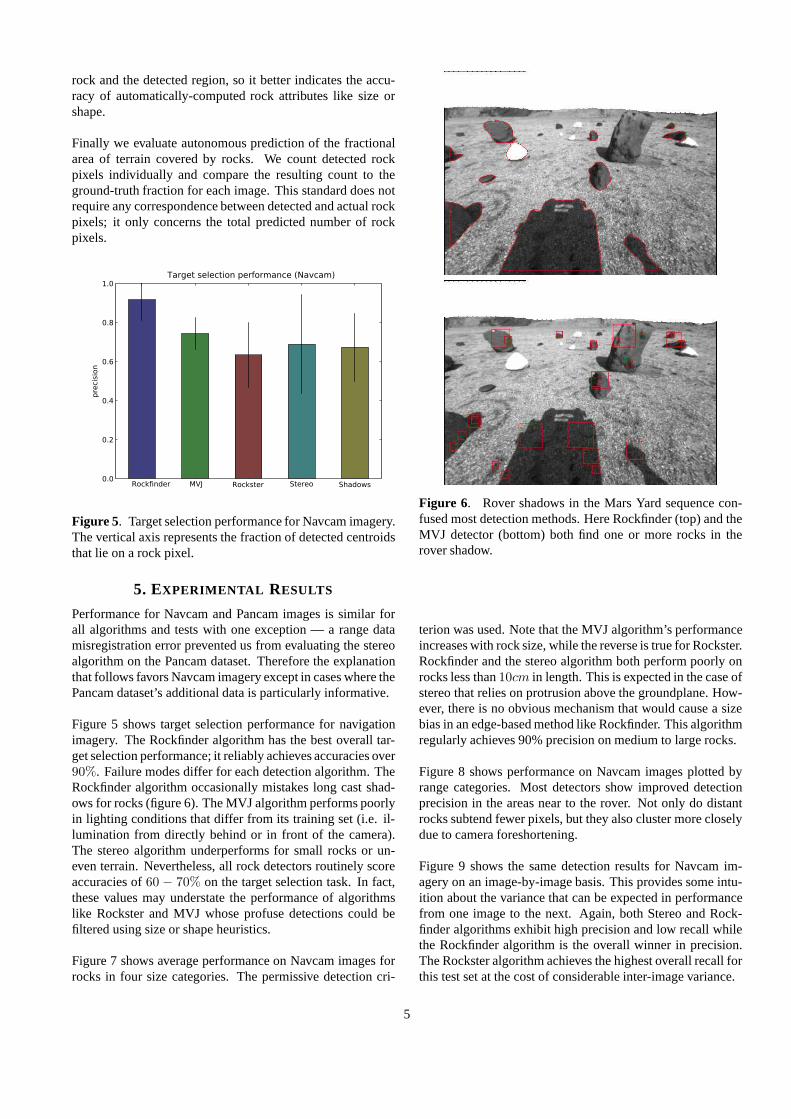
Target selection performance (Navcam)

Figure 5. Target selection performance for Navcam imagery.The vertical axis represents the fraction of detected centroidsthat lie on a rock pixel.

5. EXPERIMENTAL RESULTS

Performance for Navcam and Pancam images is similar forall algorithms and tests with one exception — a range datamisregistration error prevented us from evaluating the stereoalgorithm on the Pancam dataset. Therefore the explanationthat follows favors Navcam imagery except in cases where thePancam dataset’s additional data is particularly informative.

Figure 5 shows target selection performance for navigationimagery. The Rockfinder algorithm has the best overall tar-get selection performance; it reliably achieves accuracies over90%. Failure modes differ for each detection algorithm. TheRockfinder algorithm occasionally mistakes long cast shad-ows for rocks (figure 6). The MVJ algorithm performs poorlyin lighting conditions that differ from its training set (i.e. il-lumination from directly behind or in front of the camera).The stereo algorithm underperforms for small rocks or un-even terrain. Nevertheless, all rock detectors routinely scoreaccuracies of60 − 70% on the target selection task. In fact,these values may understate the performance of algorithmslike Rockster and MVJ whose profuse detections could befiltered using size or shape heuristics.

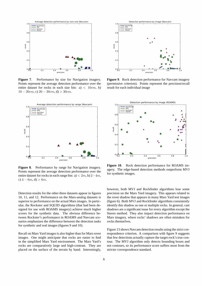
Figure 7 shows average performance on Navcam images forrocks in four size categories. The permissive detection cri-

Figure 6. Rover shadows in the Mars Yard sequence con-fused most detection methods. Here Rockfinder (top) and theMVJ detector (bottom) both find one or more rocks in therover shadow.

terion was used. Note that the MVJ algorithm’s performanceincreases with rock size, while the reverse is true for Rockster.Rockfinder and the stereo algorithm both perform poorly onrocks less than10cm in length. This is expected in the case ofstereo that relies on protrusion above the groundplane. How-ever, there is no obvious mechanism that would cause a sizebias in an edge-based method like Rockfinder. This algorithmregularly achieves 90% precision on medium to large rocks.

Figure 8 shows performance on Navcam images plotted byrange categories. Most detectors show improved detectionprecision in the areas near to the rover. Not only do distantrocks subtend fewer pixels, but they also cluster more closelydue to camera foreshortening.

Figure 9 shows the same detection results for Navcam im-agery on an image-by-image basis. This provides some intu-ition about the variance that can be expected in performancefrom one image to the next. Again, both Stereo and Rock-finder algorithms exhibit high precision and low recall whilethe Rockfinder algorithm is the overall winner in precision.The Rockster algorithm achieves the highest overall recallforthis test set at the cost of considerable inter-image variance.

5

0.0 0.2 0.4 0.6 0.8 1.0precision

0.0

0.2

0.4

0.6

0.8

1.0re

call

a b cd

a

b c dabcd

a bc

d

Average detection performance by rock size (Navcam)

RockfinderMVJ

RocksterStereo

Figure 7. Performance by size for Navigation imagery.Points represent the average detection performance over theentire dataset for rocks in each size bin: a)< 10cm, b)10 − 20cm, c) 20 − 30cm, d) > 30cm.

0.0 0.2 0.4 0.6 0.8 1.0precision

0.0

0.2

0.4

0.6

0.8

1.0

recall

a bcd

a

bcd

ab

cd

a bcd

Average detection performance by range (Navcam)

RockfinderMVJ

RocksterStereo

Figure 8. Performance by range for Navigation imagery.Points represent the average detection performance over theentire dataset for rocks in each range bin: a)< 2m, b)2−4m,c) 4 − 6m, d) > 6m.

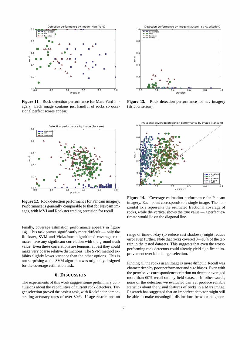
Detection results for the other three datasets appear in figures10, 11, and 12. Performance on the Mars-analog datasets issuperior to performance on the actual Mars images. In partic-ular, the Rockster and SQUID algorithms (that had been de-signed for use with ROAMS imagery) achieve much higherscores for the synthetic data. The obvious difference be-tween Rockster’s performance in ROAMS and Navcam sce-narios emphasizes the difference between the detection tasksfor synthetic and real images (figures 9 and 10).

Recall on Mars Yard images is also higher than for Mars roverimages. One might anticipate that rocks are easier to findin the simplified Mars Yard environment. The Mars Yard’srocks are comparatively large and high-contrast. They areplaced on the surface of the terrain by hand. Interestingly,

0.0 0.2 0.4 0.6 0.8 1.0precision

0.0

0.2

0.4

0.6

0.8

1.0

recall

Detection performance by image (Navcam)

RockfinderMVJ

RocksterStereo

Figure 9. Rock detection performance for Navcam imagery(permissive criterion). Points represent the precision/recallresult for each individual image

0.0 0.2 0.4 0.6 0.8 1.0precision

0.0

0.2

0.4

0.6

0.8

1.0

recall

Detection performance by image (ROAMS)

RockfinderMVJ

RocksterSQUID

Figure 10. Rock detection performance for ROAMS im-agery. The edge-based detection methods outperform MVJfor synthetic images.

however, both MVJ and Rockfinder algorithms lose someprecision on the Mars Yard imagery. This appears related tothe rover shadow that appears in many Mars Yard test images(figure 6). Both MVJ and Rockfinder algorithms consistentlyidentify this shadow as one or multiple rocks. In general, castshadows are a significant issue for every algorithm except theStereo method. They also impact detection performance onMars imagery, where rocks’ shadows are often mistaken forrocks themselves.

Figure 13 shows Navcam detection results using the strict cor-respondence criterion. A comparison with figure 9 suggeststhat few detections actually capture the target rock’s truecon-tour. The MVJ algorithm only detects bounding boxes andnot contours, so its performance score suffers most from thestricter correspondence standard.

6

0.0 0.2 0.4 0.6 0.8 1.0precision

0.0

0.2

0.4

0.6

0.8

1.0re

call

Detection performance by image (Mars Yard)

RockfinderMVJ

Rockster

Figure 11. Rock detection performance for Mars Yard im-agery. Each image contains just handful of rocks so occa-sional perfect scores appear.

0.0 0.2 0.4 0.6 0.8 1.0precision

0.0

0.2

0.4

0.6

0.8

1.0

recall

Detection performance by image (Pancam)

RockfinderMVJ

Rockster

Figure 12. Rock detection performance for Pancam imagery.Performance is generally comparable to that for Navcam im-ages, with MVJ and Rockster trading precision for recall.

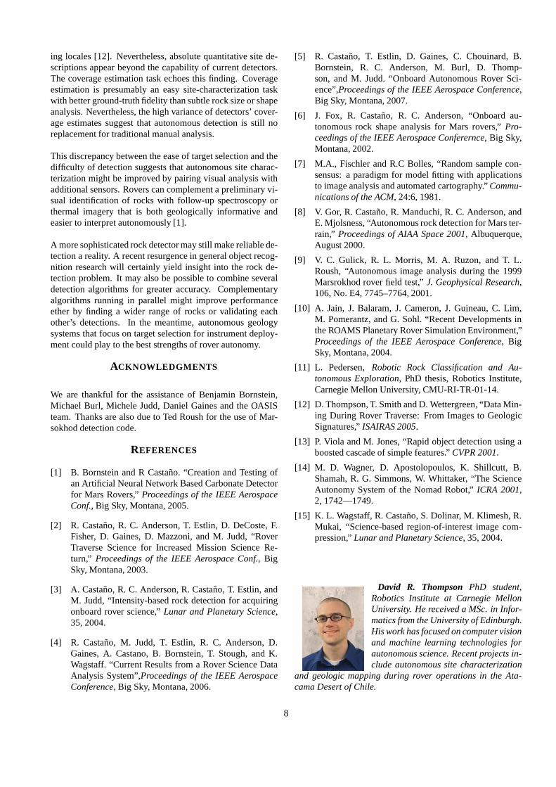
Finally, coverage estimation performance appears in figure14). This task proves significantly more difficult — only theRockster, SVM and Viola/Jones algorithms’ coverage esti-mates have any significant correlation with the ground truthvalue. Even these correlations are tenuous; at best they couldmake very coarse relative distinctions. The SVM method ex-hibits slightly lower variance than the other options. Thisisnot surprising as the SVM algorithm was originally designedfor the coverage estimation task.

6. DISCUSSION

The experiments of this work suggest some preliminary con-clusions about the capabilities of current rock detectors.Tar-get selection proved the easiest task, with Rockfinder demon-strating accuracy rates of over80%. Usage restrictions on

0.0 0.2 0.4 0.6 0.8 1.0precision

0.0

0.2

0.4

0.6

0.8

1.0

recall

Detection performance by image (Navcam - strict criterion)

RockfinderMVJ

RocksterStereo

Figure 13. Rock detection performance for nav imagery(strict criterion).

0.0 0.1 0.2 0.3 0.4 0.5

estimated

0.0

0.1

0.2

0.3

0.4

0.5

actu

al

Fractional coverage prediction performance by image (Pancam)

RockfinderMVJ

RocksterStereoSVM

Figure 14. Coverage estimation performance for Pancamimagery. Each point corresponds to a single image. The hor-izontal axis represents the estimated fractional coverageofrocks, while the vertical shows the true value — a perfect es-timate would lie on the diagonal line.

range or time-of-day (to reduce cast shadows) might reduceerror even further. Note that rocks covered0−40% of the ter-rain in the tested datasets. This suggests that even the worst-performing rock detectors could already yield significant im-provement over blind target selection.

Finding all the rocks in an image is more difficult. Recall wascharacterized by poor performance and size biases. Even withthe permissive correspondence criterion no detector averagedmore than60% recall on any field dataset. In other words,none of the detectors we evaluated can yet produce reliablestatistics about the visual features of rocks in a Mars image.Research has suggested that an imperfect detector might stillbe able to make meaningful distinctions between neighbor-

7

ing locales [12]. Nevertheless, absolute quantitative site de-scriptions appear beyond the capability of current detectors.The coverage estimation task echoes this finding. Coverageestimation is presumably an easy site-characterization taskwith better ground-truth fidelity than subtle rock size or shapeanalysis. Nevertheless, the high variance of detectors’ cover-age estimates suggest that autonomous detection is still noreplacement for traditional manual analysis.

This discrepancy between the ease of target selection and thedifficulty of detection suggests that autonomous site charac-terization might be improved by pairing visual analysis withadditional sensors. Rovers can complement a preliminary vi-sual identification of rocks with follow-up spectroscopy orthermal imagery that is both geologically informative andeasier to interpret autonomously [1].

A more sophisticated rock detector may still make reliable de-tection a reality. A recent resurgence in general object recog-nition research will certainly yield insight into the rock de-tection problem. It may also be possible to combine severaldetection algorithms for greater accuracy. Complementaryalgorithms running in parallel might improve performanceether by finding a wider range of rocks or validating eachother’s detections. In the meantime, autonomous geologysystems that focus on target selection for instrument deploy-ment could play to the best strengths of rover autonomy.

ACKNOWLEDGMENTS

We are thankful for the assistance of Benjamin Bornstein,Michael Burl, Michele Judd, Daniel Gaines and the OASISteam. Thanks are also due to Ted Roush for the use of Mar-sokhod detection code.

REFERENCES

[1] B. Bornstein and R Castano. “Creation and Testing ofan Artificial Neural Network Based Carbonate Detectorfor Mars Rovers,”Proceedings of the IEEE AerospaceConf., Big Sky, Montana, 2005.

[2] R. Castano, R. C. Anderson, T. Estlin, D. DeCoste, F.Fisher, D. Gaines, D. Mazzoni, and M. Judd, “RoverTraverse Science for Increased Mission Science Re-turn,” Proceedings of the IEEE Aerospace Conf., BigSky, Montana, 2003.

[3] A. Castano, R. C. Anderson, R. Castano, T. Estlin, andM. Judd, “Intensity-based rock detection for acquiringonboard rover science,”Lunar and Planetary Science,35, 2004.

[4] R. Castano, M. Judd, T. Estlin, R. C. Anderson, D.Gaines, A. Castano, B. Bornstein, T. Stough, and K.Wagstaff. “Current Results from a Rover Science DataAnalysis System”,Proceedings of the IEEE AerospaceConference, Big Sky, Montana, 2006.

[5] R. Castano, T. Estlin, D. Gaines, C. Chouinard, B.Bornstein, R. C. Anderson, M. Burl, D. Thomp-son, and M. Judd. “Onboard Autonomous Rover Sci-ence”,Proceedings of the IEEE Aerospace Conference,Big Sky, Montana, 2007.

[6] J. Fox, R. Castano, R. C. Anderson, “Onboard au-tonomous rock shape analysis for Mars rovers,”Pro-ceedings of the IEEE Aerospace Conferernce, Big Sky,Montana, 2002.

[7] M.A., Fischler and R.C Bolles, “Random sample con-sensus: a paradigm for model fitting with applicationsto image analysis and automated cartography.”Commu-nications of the ACM, 24:6, 1981.

[8] V. Gor, R. Castano, R. Manduchi, R. C. Anderson, andE. Mjolsness, “Autonomous rock detection for Mars ter-rain,” Proceedings of AIAA Space 2001, Albuquerque,August 2000.

[9] V. C. Gulick, R. L. Morris, M. A. Ruzon, and T. L.Roush, “Autonomous image analysis during the 1999Marsrokhod rover field test,”J. Geophysical Research,106, No. E4, 7745–7764, 2001.

[10] A. Jain, J. Balaram, J. Cameron, J. Guineau, C. Lim,M. Pomerantz, and G. Sohl. “Recent Developments inthe ROAMS Planetary Rover Simulation Environment,”Proceedings of the IEEE Aerospace Conference, BigSky, Montana, 2004.

[11] L. Pedersen,Robotic Rock Classification and Au-tonomous Exploration, PhD thesis, Robotics Institute,Carnegie Mellon University, CMU-RI-TR-01-14.

[12] D. Thompson, T. Smith and D. Wettergreen, “Data Min-ing During Rover Traverse: From Images to GeologicSignatures,”ISAIRAS 2005.

[13] P. Viola and M. Jones, “Rapid object detection using aboosted cascade of simple features.”CVPR 2001.

[14] M. D. Wagner, D. Apostolopoulos, K. Shillcutt, B.Shamah, R. G. Simmons, W. Whittaker, “The ScienceAutonomy System of the Nomad Robot,”ICRA 2001,2, 1742—1749.

[15] K. L. Wagstaff, R. Castano, S. Dolinar, M. Klimesh, R.Mukai, “Science-based region-of-interest image com-pression,”Lunar and Planetary Science, 35, 2004.

David R. Thompson PhD student,Robotics Institute at Carnegie MellonUniversity. He received a MSc. in Infor-matics from the University of Edinburgh.His work has focused on computer visionand machine learning technologies forautonomous science. Recent projects in-clude autonomous site characterization

and geologic mapping during rover operations in the Ata-cama Desert of Chile.

8

Dr. Rebecca Castano Supervisor, Ma-chine Learning Systems group at JPL,OASIS Technical team lead. She re-ceived her Ph.D. in Electrical Engineer-ing from the Universiry of Illinois withher dissertion in the area of computer vi-sion. Dr. Castano has been advancingthe state of the art in onboard science

analysis methods for the part eight years and has been leadauthor on numerous publications in this field. Her researchinterests include machine learning, computer vision and pat-tern recognition.

9