Performance Evaluation of Heterogeneous Network Scenarios

Performance Evaluation of Heterogeneous

Network Scenarios

Alessio Botta, Donato Emma, Salvatore Guadagno, and Antonio Pescape∗

Abstract

Packet loss, delay and jitter degrade the quality of services like VoIP(Voice over IP) or Video Streaming over IP networks. In real networks, anexperimental measure of these parameters is fundamental in the planningprocess of new services over novel network infrastructures.

Furthermore, currently networks are complex heterogeneous systems(in terms of access network technologies, end-users’ devices, OperatingSystems and finally end-users’ application). This heterogeneity exacer-bates even more the need of a real assessment of the Quality of Servicemetrics. Stepping fro this consideration, in this Chapter we provide anempirical performance study of real heterogeneous wireless network withrespect to delay, jitter, throughput and packet loss, in UDP and TCPenvironments, by using the innovative tool D-ITG (Distributed InternetTraffic Generator).

We also use the concept of “Service Condition” as a mechanism to copewith issues related to dynamically changing network service scenario andto formally define a parametric and systemic approach to the performanceevaluation.

Results presented in this Report can be used as performance referencesfor development of wireless communication applications over multi-serviceheterogeneous networks.

Indeed, we perform a large set of measurements with a wide set ofhardware. Then we take the results of our measurements and by analyzingthe similarities and the differences we understand what we can generalizeand what not. We investigate the impact of mechanisms and protocolson the performance metrics and we try to prove which protocol elementis a limiting factor or which devices characteristics affect the measuredmetrics. In addition, thanks to the wide range of provided results (as wellas the public traffic traces, available on request), a reader could actuallymake use of the information provided in this Report for his purposes.

More precisely, this Report presents results of our performance evalu-ation activities in the following scenario:

∗D. Emma, A. Pescape, and G. Ventre are with the Dipartimento di Informatica e Sis-temistica, Universita di Napoli “Federico II”, Naples, Italy. {doemma,pescape}@unina.it. A.Botta and S. Guadagno are with the Consorzio Interuniversitario Nazionale per l’Informatica,Naples (Italy), {abotta, sguadagno}@napoli.consorzio-cini.it.

1

• HetPerf (Heterogeneous Networks Performance): this framework presentsexperimental results related to heterogeneous networks where bothwireless local area networks and cellular networks are present. Westudy the performance in this integrated and heterogeneous scenarioorganizing our results in the following way:

– Wireless Local Area Networks (Wi-Fi WLAN 802.11b)

– Wireless Wide Area Networks (GPRS and UMTS)

• HandPerf (Vertical Handoff Performance): this framework presentsexperimental results related to an architecture for seamless handoffs.

1 Introduction

In the last years network capacity has increased at a dramatic rate. At thesame time the proliferation of the web has resulted in an exponential increasein the number of “surfing users” supported by the Internet. These users are be-coming increasingly sophisticated and demand high-bandwidth, low-delay net-work services at affordable prices. Currently, this services’ request is made overnew “heterogeneous, integrated and mobile” IP (Internet Protocol) networks.Always-on connectivity, location-awareness, and environment-aware productsare some of the new paradigms over heterogeneous wireless networks. Smartdevices, portable devices, wireless communications appear to be the underlyingprinciples of a new revolution in technology. Pervasive computing deals witha wide range of information access methods enabled by mobility, wireless tech-nologies, small embedded systems and broadband technologies [1]. Integrationof fixed and wireless access (local and geographic) to IP networks presents acost effective and efficient way to provide seamless end-to-end connectivity andubiquitous access in a market where demands of mobile Internet have grownrapidly and predicted to generate billions of dollars in revenue. In this en-vironment, among the many factors that determine the feasibility of a givennetwork scenario for the given set of application requirements, there is networkperformance. Network performance is generally affected by different aspects atthe physical, data link, network, and transport layers. In a generic real net-work and in particular in a heterogeneous scenario, it is extremely difficult (i)to define a general framework for empirical performance evaluation and (ii) todetermine the causes of the experimented performance. This Chapter focuseson the area of performance evaluation of heterogeneous wireless networks fromthe application level point of view.

By using the same approach adopted in previous Chapters, the experimentalanalysis has been carried out over large but controlled network environments.Therefore, also in the case of performance evaluation of heterogeneous wirelessnetworks we used experimental test-beds present in our laboratories. Sincewe also measured scenario where UMTS and GPRS networks are present, weattached our experimental test-beds to Telecom Operators networks. These arethe only two cases where the access networks are out of our control. Therefore,

2

as for the analyzed “Service Condition” we tested real heterogeneous wirelessnetworks made a number of complex combination by:

• Access Networks: Ethernet, 802.11b, GPRS, and UMTS

• End User Devices: Workstation, Personal Computer, Laptop, Notebook,and Personal Digital Assistant (PDA)

• Operating Systems: Unix, Linux, Windows, and Linux Familiar

Over the depicted scenario we tested the behavior of both UDP and TCP.In order to define a systemic measurement approach we introduced a net-

work performance methodology dividing our experimentation on several trafficclasses. The performance evaluation study has been performed by followingsome of the indications of IP Performance Metrics (IPPM) IETF Working Group[13] and by adopting the guidelines reported in [14]. The network behavior hasbeen studied by using D-ITG (Distributed Internet Traffic Generator) . Wepresent our experimental results and at the same time we analyze and compareour results with respect to theoretical assumptions on wireless performance be-havior carried out in [2].

As said, we show how to use the “Service Condition” concept to cope withthe issues of a performance evaluation framework in a heterogeneous wirelessenvironment. More precisely, first we present and discuss results of a completeperformance evaluation of a heterogeneous wireless scenario. In this first studywe show the achieved performance as a function of Access Network, End-UserDevice, Operating System, and Application (TCP or UDP). We called thisframework HetPerf. Second, we present results of an experimental analysis of aheterogeneous scenario where vertical handoffs are present. In practice, in thiscase we study the performance of “Service Conditions” that present the samevalues of End-User Device, Operating System, and Application but differentvalues in terms of Access Networks. We called this second framework HandPerf.

Thanks to this performance evaluation study:

• we are in charge of to demonstrate the goodness of the “Service Condition”concept in the field of network measurements;

• we provide a complete study of heterogeneous wireless networks in terms ofthroughput, delay (OWD and RTT), packet loss, and jitter. It representsa real assessment of QoS metrics over heterogeneous wireless networks;

• we present a clear definition of which system’s elements are responsible ofnetwork performances degradation and how the used different protocolsimpact on the observed network performance.

1.1 Test-bed Infrastructure, Tools and ExperimentalMethodology

The goal of our analysis is an empirical performance characterization of realheterogeneous networks in which several wireless links are present. In order to

3

Figure 1: The Experimental Test-bed Infrastructure: Real Network

Transmitting Host Receiving HostNetwork

D-ITG D-ITG

12 3 4

Figure 2: The Experimental Test-bed Infrastructure: Conceptual Schema

pursue this objective a set of experimental setups with similar characteristicshas been chosen (see Figure 1).

The first step towards the definition of a systemic measurement approach isthe definition of a network conceptual schema. All tests can be collapsed in asame general schema, depicted in figure 2, where two communication entities,a D-ITG transmitter and a D-ITG receiver, are directly connected through anIP network channel. Indeed, the tests differ for the type of used network, itsconfiguration, the type of host that executes the D-ITG platform, and used Op-erating Systems. By changing these parameters we tested several strictly related“Service Conditions”. In figure 2 the conceptual schema of the experimentaltest-bed is depicted.

In this preliminary study, others parametric elements, like generated trafficpatterns have not been changed. We used only periodical sources, with fixedPacket Size (PS) and fixed Inter-Departure Times (IDT) between packets sinceour intention for this study was mainly to focus on the impact of heterogeneity.

In our performance evaluation we organize our measurements such that todistinguish three types of traffic conditions:

• low traffic load (≤ 1.2Mbps): in our scenario low traffic load means atraffic state in which we are far from the saturated 802.11b wireless channel

4

condition.

• medium traffic load (≤ 4.0Mbps): for medium traffic load we mean atraffic state in which we are close to the saturated 802.11b wireless channelcondition.

• high traffic load (≤ 10Mbps): in the case of high traffic load we have atraffic state in which we are in the saturated 802.11b wireless channel con-dition (i.e. every station has always a packet ready for the transmission).

These three traffic conditions are related to three different real traffic loads wherewe used different packet size. Indeed, in the first traffic profile we used PS equalto {64, 128, 256, 512, 1024, 1500} bytes and IDT equal to 1

100 (according to lowtraffic load). In the second traffic profile we used PS equal to {64, 128, 256,512} bytes and IDT equal to 1

1000 (according to medium traffic load). Finally inthe third traffic profile we adopted PS equal to {64, 128} bytes and IDT equalto 1

10000 (according to high traffic load).

2 HetPerf

As for the performance evaluation of the scenario that we called “HetPerf ”, intable 1 the complete set of parametric elements used in our tests is summarized.In addition, in the case of an ad-hoc scenario, we have experimented moreconfigurations, allowing the two communicating hosts to move at various mutualdistances: we tested a mobile environment using roaming user in three classesof end-to-end mutual distances (d ≤ 5 m, 5 m ≤ d ≤ 10 m, 10 m ≤ d ≤ 15 m)(Figure 3).

For every traffic condition presented in the previous Paragraph, we organizedthe data in three types of configurations: (i) a classic configuration, with onlylaptop and workstation devices, (ii) a second configuration, where the transmit-ting host is always a Palmtop and (iii) a third configuration, where the receivinghost is always a Palmtop.

In order to characterize a system like that one depicted in figure 2, weused the following QoS parameters by using the recommendations of IPPMworking group [13]: (i) the (source/destination)-bandwidth (UDP and TCPprotocols); (ii) the delay (UDP only); (iii) the jitter (UDP only) and finally(iv) the packet loss (UDP only). For each measured parameter, several trialshave been performed in the same operating conditions. The values reported inthe following graphics represent a mean value across twenty test repetitions. Inour opinion, achieved results represent a good starting point. Indeed, duringour current study we are experimenting similar results in other heterogeneousnetwork configurations. Beside the statistics provided by D-ITG, we used nstatto gather IP, UDP and TCP statistics aggregated across all interfaces, so as tocheck for unexpected network activity during the experiments.

5

Figure 3: Physical Layout in the case of Experiments with Mobile node

Table 1: “Service Conditions” componentsTest-bed Element Variables Values

Protocol {UDP, TCP}1 - D-ITG Inter-Departure Size IDT={ 1

100, 1

1000, 1

10000} s

Packet Size PS={64, 128, 256, 512,1024, 1500} bytes

2 - Tx-Host End users’ device {Workstation, Laptop, Palmtop}Network Scenario {Wired2Wired, Wired2Wireless,

3 - Network Wireless2Wireless, with andwithout Access Point(AP), . . . }

4 - Rx-Host End users’ device {Workstation, Laptop, Palmtop}5 - Operating System End users’ OSs {Windows XP, Linux,

Linux Familiar}

6

Table 2: Picture LegendNetwork Scenario Description

wired2wired Connection between two workstation throughan Ethernet 10/100 Mbps network

wired2wireless Connection between the workstation and thelaptop/palmtop through AP

wireless2wireless (AP) Connection between laptop and palmtopthrough AP

wireless2wireless (d ≤ x) Connection between laptop and palmtopin ad-hoc mode in a range of x meters

Table 3: Technical details on the experimental setupDevice Description

Laptop1 IBM T23, Mobile Intel PIII 1133 Mhz,Main Memory 128 MB, Cache 256 KB,O.S. Linux Red Hat 9.0 kernel 2.4.20-18.9

Laptop2 Acer TravelMate 351 TE: PIII 700 Mhz,Main Memory 128 MB

Workstation1 PC sender, Intel PII 850 Mhz,Main Memory 128 MB, Cache 256 KB,dual boot Operating Systems: Linux(2.4),Windows XP Professional Service Pack 1

Workstation2 PC receiver, Intel C 400 Mhz, Main Memory 64 MB,Cache 128 KB, O.S. Linux(2.4)

Palmtop Compaq iPAQ H3850, Intel StrongARM 206 Mhz,Main Memory 64 MB, Flash ROM 32 MB,O.S. Linux FAMILIAR kernel 2.4.18

Access Point Orinoco Ap1000, 11Mbps (802.11b),Multi Channel support

Wireless LAN cards WiFi ORINOCO 11Mbps GOLD

7

200 400 600 800 1000 1200 14000

200

400

600

800

1000

1200

packet size (bytes)

thro

ughp

ut (k

bps)

Palmtop−>Laptop − Sender Side − IDT 100

wireless−to−wireless (AP)wired−to−wireless (AP)wireless ad−hoc (d<5m)wireless ad−hoc (5m<d<10m)wireless ad−hoc (10m<d<15m)

200 400 600 800 1000 1200 14000

200

400

600

800

1000

1200

packet size (bytes)

thro

ughp

ut (k

bps)

Palmtop−>Laptop − Receiver Side − IDT 100


Figure 4: Throughput analysis at sender (left) and receiver (right) side for IDT= 1

100 s in the case of UDP

2.1 Experimentation with Wireless Local Area Network

In this section measures obtained in the analyzed “Service Conditions” arepresented. We organize our results showing the throughput, delay, jitter andpacket loss measured in the following subsections. In table 2 the completereference for the legend used in the following graphs is reported whereas intable 3 details on devices used are depicted.

2.1.1 Throughput Analysis

We step from showing and analyzing of results for low load traffic condition,then we present the results for medium and, finally, we show the results for hightraffic load. As far as the throughput, a deep results analysis is reported inSection 2.1.5. In all following figures (except for figures 4 and 5), the first row isrelated to a situation in which the communication entities are two workstations,one workstation and one laptop, or two laptops; instead, the others two rowsare related to a scenario in which the transmitter (second row) or the receiving(third row) host is always a Palmtop, while the transmitting/receiving one isa workstation (wired element) or a laptop (wireless element). First column ofeach figure represents the behavior observed by the transmitting host, while thesecond one represents the behavior observed by receiving host.

Low traffic load In the case of low traffic load we are far from the saturatedwireless channel condition. Test results for low traffic load are depicted in fig-ures 4 and 5. In this case, we show only the graphics related to the behaviorof the Palmotp2Laptop communication because it is the only situation wherewe can appreciate some very low performance degradation: in the case of Lap-top2Laptop and Laptop2Palmtop communications both in the UDP and TCPscenario the sent throughput is equal to the received one for each packet size.

The throughput at sender and receiver side is reported in figures 4 and 5,using respectively UDP and TCP transport protocols. A precise results analysis

8

200 400 600 800 1000 1200 14000

200

400

600

800

1000

1200

packet size (bytes)

thro

ughp

ut (k

bps)



200 400 600 800 1000 1200 14000

200

400

600

800

1000

1200

packet size (bytes)

thro

ughp

ut (k

bps)




100 s in the case of TCP

is reported in Section 2.1.5.

Medium traffic load The test results for medium traffic load are depictedin figures 6 and 7. In this case we are close to the saturated wireless channelcondition. In order to quantify the proximity to the saturated channel condition,in the diagrams of the throughput it has been brought back also the diagramobtained from the Bianchi theoretical model [2]. In [2] a simple analytical modelto compute the saturation throughput performance of the 802.11 is presented.The model assumes a finite number of terminals and ideal channel conditions andit is suited for any access scheme employed. The model shows that performanceof the basic access method strongly depends on the system parameters, mainlypacket size dimension and number of stations in the wireless network. Suchmodel gives us a bound to the maximum traffic load that can cross the channelat the MAC layer of the ISO/OSI stack, therefore it supplies a useful bound forthe traffic at the upper layer. Using our experimental results, we can also providea practical validation of the Bianchi theoretical model (see Section 2.1.5).

In this load condition it turns out with more evidence the dependency fromthe host typology and the used transport protocol. TCP still demonstratesof being more sensitive to the losses respect to UDP. However, regarding theprevious case we can observe the greater sensitivity respect to packet dimensionof the wireless configurations, especially of those with the Palmtop. A detailedresults analysis is reported in Section 2.1.5.

High traffic load Test results for high traffic load are depicted in figures 8and 9. In this case we are in the saturated wireless channel condition. Withrespect to previous cases we have analyzed a transmission condition where thepacket size is equal to 64 bytes and equal to 128 bytes. Indeed, for whicheverpacket dimension the channel turns out saturated: longer packets carry to agreater channel busy time for delivered or collided packet, and it only leads to agreater number of losses from the sender side for network interface saturation.

9

100 150 200 250 300 350 400 450 5000

500

1000

1500

2000

2500

3000

3500

4000

4500

5000

5500

packet size (bytes)

thro

ughp

ut (k

bps)

Laptop−>Laptop − Sender Side − IDT 1000

wireless−to−wireless (AP)wired−to−wireless (AP)wireless ad−hoc (d<5m)wireless ad−hoc (5m<d<10m)wireless ad−hoc (10m<d<15m)Bianchi Model

100 150 200 250 300 350 400 450 5000

500

1000

1500

2000

2500

3000

3500

4000

4500

5000

5500

packet size (bytes)

thro

ughp

ut (k

bps)

Laptop−>Laptop − Receiver Side − IDT 1000


100 150 200 250 300 350 400 450 5000

500

1000

1500

2000

2500

3000

3500

4000

4500

5000

5500

packet size (bytes)

thro

ughp

ut (k

bps)

Laptop−>Palmtop − Sender Side − IDT 1000


100 150 200 250 300 350 400 450 5000

500

1000

1500

2000

2500

3000

3500

4000

4500

5000

5500

packet size (bytes)

thro

ughp

ut (k

bps)

Laptop−>Palmtop − Receiver Side − IDT 1000


100 150 200 250 300 350 400 450 5000

500

1000

1500

2000

2500

3000

3500

4000

4500

5000

5500

packet size (bytes)

thro

ughp

ut (k

bps)


wireless−to−wireless (AP)wireless−to−wired (AP)wireless ad−hoc (d<5m)wireless ad−hoc (5m<d<10m)wireless ad−hoc (10m<d<15m)Bianchi Model

100 150 200 250 300 350 400 450 5000

500

1000

1500

2000

2500

3000

3500

4000

4500

5000

5500

packet size (bytes)

thro

ughp

ut (k

bps)





10

100 150 200 250 300 350 400 450 5000

500

1000

1500

2000

2500

3000

3500

4000

4500

5000

5500

packet size (bytes)

thro

ughp

ut (k

bps)



100 150 200 250 300 350 400 450 5000

500

1000

1500

2000

2500

3000

3500

4000

4500

5000

5500

packet size (bytes)

thro

ughp

ut (k

bps)



100 150 200 250 300 350 400 450 5000

500

1000

1500

2000

2500

3000

3500

4000

4500

5000

5500

packet size (bytes)

thro

ughp

ut (k

bps)



100 150 200 250 300 350 400 450 5000

500

1000

1500

2000

2500

3000

3500

4000

4500

5000

5500

packet size (bytes)

thro

ughp

ut (k

bps)



100 150 200 250 300 350 400 450 5000

500

1000

1500

2000

2500

3000

3500

4000

4500

5000

5500

packet size (bytes)

thro

ughp

ut (k

bps)



100 150 200 250 300 350 400 450 5000

500

1000

1500

2000

2500

3000

3500

4000

4500

5000

5500

packet size (bytes)

thro

ughp

ut (k

bps)





11

64 1280

1000

2000

3000

4000

5000

6000

7000

8000

9000

10000

11000

packet size (bytes)

thro

ughp

ut (k

bps)


Bianchi Modelwireless−to−wireless (AP)wired−to−wireless (AP)wireless ad−hoc (d<5m)wireless ad−hoc (5m<d<10m)wireless ad−hoc (10m<d<15m)

64 1280

1000

2000

3000

4000

5000

6000

7000

8000

9000

10000

11000

packet size (bytes)

thro

ughp

ut (k

bps)



64 1280

1000

2000

3000

4000

5000

6000

7000

8000

9000

10000

11000

packet size (bytes)

thro

ughp

ut (k

bps)



64 1280

1000

2000

3000

4000

5000

6000

7000

8000

9000

10000

11000

packet size (bytes)

thro

ughp

ut (k

bps)



64 1280

1000

2000

3000

4000

5000

6000

7000

8000

9000

10000

11000

packet size (bytes)

thro

ughp

ut (k

bps)


Bianchi Modelwireless−to−wireless (AP)wireless−to−wired (AP)wireless ad−hoc (d<5m)wireless ad−hoc (5m<d<10m)wireless ad−hoc (10m<d<15m)

64 1280

1000

2000

3000

4000

5000

6000

7000

8000

9000

10000

11000

packet size (bytes)

thro

ughp

ut (k

bps)





12

64 1280

1000

2000

3000

4000

5000

6000

7000

8000

9000

10000

11000

packet size (bytes)

thro

ughp

ut (k

bps)



64 1280

1000

2000

3000

4000

5000

6000

7000

8000

9000

10000

11000

packet size (bytes)

thro

ughp

ut (k

bps)



64 1280

1000

2000

3000

4000

5000

6000

7000

8000

9000

10000

11000

packet size (bytes)

thro

ughp

ut (k

bps)



64 1280

1000

2000

3000

4000

5000

6000

7000

8000

9000

10000

11000

packet size (bytes)

thro

ughp

ut (k

bps)



64 1280

1000

2000

3000

4000

5000

6000

7000

8000

9000

10000

11000

packet size (bytes)

thro

ughp

ut (k

bps)



64 1280

1000

2000

3000

4000

5000

6000

7000

8000

9000

10000

11000

packet size (bytes)

thro

ughp

ut (k

bps)





13

The organization of the diagrams is the same one of the previous cases, the onlydifference is in having brought back the transmission and reception plots usinghistogram diagrams (in this case we have changed the figures layout because wehave only two packet dimensions). It is interesting to notice the behavior of UDPand TCP in the several analyzed configurations: TCP reacts to the saturationcondition limiting the demanded transmission bandwidth, while UDP endures ahighest packet loss. This behavior is caused from the presence of a flow-controlmechanism in the first protocol, and from the ability to the congestion controlof TCP to optimize the use of a high loaded channel. Also in this case a deepanalysis is reported in Section 2.1.5.

2.1.2 Delay Analysis

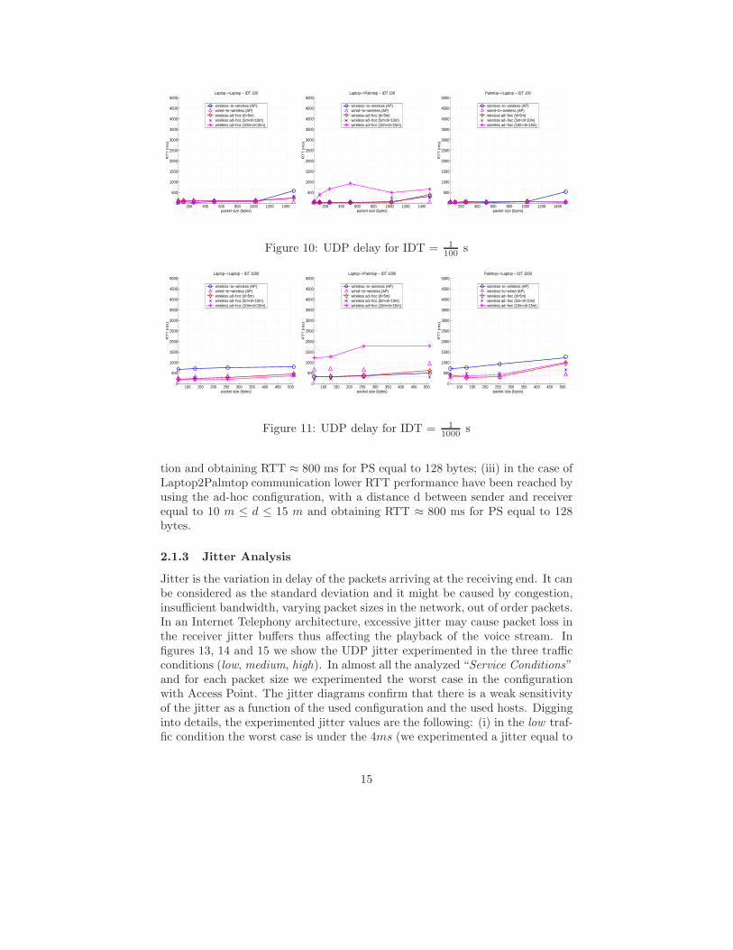
Delay is the amount of time that a packet takes to travel from the senders appli-cation to reach the receivers destination application. For example, in an InternetTelephony scenario, one-way delay requirement is stringent for VoIP to main-tain good interaction between end-nodes. In order to have an upper bound forthe one way delay we measured the Round Trip Time (RTT). This is due to: (i)we perform our measurement activities in the field of IPPM recommendations[13]; (ii) our measurements are carried out over wireless local links and not overgeographical wireless links. The organization of the diagrams follows the samelayout of the previous sections. As far as RTT thanks to our experimentation welearned that: (i) in the case of low traffic condition the configuration with Ac-cess Point presents the lowest performance for high packet size (for PS equal to1500 bytes we measured RTT ≈ 500 ms); (ii) the previous statement is not truein the case of Laptop2Palmtop configuration where we experimented the low-est performance in the case of ad-hoc configuration, with a distance d betweensender and receiver equal to 10 m ≤ d ≤ 15 m (in this case we measured RTTuntil to 1000 ms). In the case of medium and high traffic condition we experi-mented the same behavior described for low traffic condition with same trend ata much high values. More precisely, as far as medium traffic condition: (i) theconfiguration with Access Point remains the scenario with lowest performancein the case of Laptop2Laptop and Palmtop2Laptop communications; (ii) in thecase of Laptop2Laptop communications the RTT for the configuration with Ac-cess Point is under the 900 ms (700 ms ≤ RTT ≤ 900 ms); (iii) in the caseof Palmtop2Laptop communications the RTT for the configuration with AccessPoint reaches RTT ≈ 500 ms for PS equal to 1500 bytes; (iv) in the case of Lap-top2Palmtop configuration we experimented the lowest performance in the caseof ad-hoc configuration, with a distance d between sender and receiver equal to10 m ≤ d ≤ 15 m (in this case we measured an 1300 ms ≤ RTT ≤ 1800 ms).As far as high traffic condition we have the same behavior of the medium traf-fic condition with the following differences in terms of achieved results: (i) inthe case of Laptop2Laptop communication lower RTT performance have beenreached by using the Access Point configuration and obtaining RTT ≈ 700 msfor PS equal to 128 bytes; (ii) in the case of Palmtop2Laptop communicationlower RTT performance have been reached by using the Access Point configura-

14

200 400 600 800 1000 1200 14000

500

1000

1500

2000

2500

3000

3500

4000

4500

5000

packet size (bytes)

RT

T (

ms)

Laptop−>Laptop − IDT 100


200 400 600 800 1000 1200 14000

500

1000

1500

2000

2500

3000

3500

4000

4500

5000

packet size (bytes)

RT

T (

ms)

Laptop−>Palmtop − IDT 100


200 400 600 800 1000 1200 14000

500

1000

1500

2000

2500

3000

3500

4000

4500

5000

packet size (bytes)

RT

T (

ms)

Palmtop−>Laptop − IDT 100


Figure 10: UDP delay for IDT = 1100 s

100 150 200 250 300 350 400 450 5000

500

1000

1500

2000

2500

3000

3500

4000

4500

5000

packet size (bytes)

RT

T (

ms)



100 150 200 250 300 350 400 450 5000

500

1000

1500

2000

2500

3000

3500

4000

4500

5000

packet size (bytes)

RT

T (

ms)



100 150 200 250 300 350 400 450 5000

500

1000

1500

2000

2500

3000

3500

4000

4500

5000

packet size (bytes)

RT

T (

ms)


wireless−to−wireless (AP)wireless−to−wired (AP)wireless ad−hoc (d<5m)wireless ad−hoc (5m<d<10m)wireless ad−hoc (10m<d<15m)


tion and obtaining RTT ≈ 800 ms for PS equal to 128 bytes; (iii) in the case ofLaptop2Palmtop communication lower RTT performance have been reached byusing the ad-hoc configuration, with a distance d between sender and receiverequal to 10 m ≤ d ≤ 15 m and obtaining RTT ≈ 800 ms for PS equal to 128bytes.

2.1.3 Jitter Analysis

Jitter is the variation in delay of the packets arriving at the receiving end. It canbe considered as the standard deviation and it might be caused by congestion,insufficient bandwidth, varying packet sizes in the network, out of order packets.In an Internet Telephony architecture, excessive jitter may cause packet loss inthe receiver jitter buffers thus affecting the playback of the voice stream. Infigures 13, 14 and 15 we show the UDP jitter experimented in the three trafficconditions (low, medium, high). In almost all the analyzed “Service Conditions”and for each packet size we experimented the worst case in the configurationwith Access Point. The jitter diagrams confirm that there is a weak sensitivityof the jitter as a function of the used configuration and the used hosts. Digginginto details, the experimented jitter values are the following: (i) in the low traf-fic condition the worst case is under the 4ms (we experimented a jitter equal to

15

64 1280

500

1000

1500

2000

2500

3000

3500

4000

4500

5000

packet size (bytes)

RT

T (

ms)



64 1280

500

1000

1500

2000

2500

3000

3500

4000

4500

5000

packet size (bytes)

RT

T (

ms)



64 1280

500

1000

1500

2000

2500

3000

3500

4000

4500

5000

packet size (bytes)

RT

T (

ms)




2.5ms in the Laptop2Laptop configuration); (ii) in the medium traffic conditionthe worst case is under the 8ms (we experimented a jitter equal to 2.5ms in theLaptop2Laptop configuration); (iii) in the high traffic condition the worst case isunder the 4ms (we experimented a jitter equal to 0.5ms in the Laptop2Palmtopconfiguration). Highest values of the jitter have been experimented in the caseof medium traffic load for high values of packet size (512bytes) and for commu-nications between Laptop2Palmtop and Palmtop2Laptop: this behavior is dueto low capacity of Palmtops. The jitter behavior is associated to packet lossbehavior and experimented throughput. We present the packet loss trend inthe subsection 2.1.4.

200 400 600 800 1000 1200 14000

1

2

3

4

5

6

7

8

9

10

packet size (bytes)

jitte

r (m

s)



200 400 600 800 1000 1200 14000

1

2

3

4

5

6

7

8

9

10

packet size (bytes)

jitte

r (m

s)



200 400 600 800 1000 1200 14000

1

2

3

4

5

6

7

8

9

10

packet size (bytes)

jitte

r (m

s)Palmtop−>Laptop − IDT 100


Figure 13: UDP jitter for IDT = 1100 s

2.1.4 Packet Loss Analysis

Packet loss is a measure of packets discarded deliberately or non-deliberatelyby intermediate links, nodes and end-systems along a given transmission pathbetween sender and receiver. In this section we present a packet loss analysisfollowing the same “modus operandi” of the previous section: (i) UDP scenario;(ii) different PSs; (iii) different IDTs; (iv) different network technologies andend nodes. Figure 16 shows the UDP packet loss for IDT = 1

100 s. Except some

16

100 150 200 250 300 350 400 450 5000

1

2

3

4

5

6

7

8

9

10

packet size (bytes)

jitte

r (m

s)Laptop−>Laptop − IDT 1000


100 150 200 250 300 350 400 450 5000

1

2

3

4

5

6

7

8

9

10

packet size (bytes)

jitte

r (m

s)



100 150 200 250 300 350 400 450 5000

1

2

3

4

5

6

7

8

9

10

packet size (bytes)

jitte

r (m

s)



Figure 14: UDP jitter IDT = 11000 s

64 1280

1

2

3

4

5

6

7

8

9

10

packet size (bytes)

jitte

r (m

s)



64 1280

1

2

3

4

5

6

7

8

9

10

packet size (bytes)

jitte

r (m

s)



64 1280

1

2

3

4

5

6

7

8

9

10

packet size (bytes)

jitte

r (m

s)



Figure 15: UDP jitter for IDT = 110000 s

17

200 400 600 800 1000 1200 14000

0.5

1

1.5

2

2.5

3

3.5

4

4.5

5

packet size (bytes)

pa

cke

t lo

ss (

%)



200 400 600 800 1000 1200 14000

0.5

1

1.5

2

2.5

3

3.5

4

4.5

5

packet size (bytes)

pa

cke

t lo

ss (

%)



200 400 600 800 1000 1200 14000

0.5

1

1.5

2

2.5

3

3.5

4

4.5

5

packet size (bytes)

pa

cke

t lo

ss (

%)



Figure 16: UDP packet loss for IDT = 1100 s

singularities in the ad-hoc configuration with 10 m ≤ d ≤ 15 m, all considered“Service Conditions” showed a packet loss under the 0.5% and substantiallyequal to 0. More precisely, only when at receiver side a Palmtop is present andthe packet size is lower than 512bytes we measured a packet loss diverse from0 and in all case lower than 0.5%. At the opposite site, Figure 17 and Figure18 show dramatic values for the packet loss: in the case of medium and hightraffic load the configuration with Access Point presents the lowest performancein terms of packet loss. More precisely, we experimented: (i) UDP packet lossfor IDT = 1

1000 s up to 70%; (ii) UDP packet loss for IDT = 110000 s up to 95%.

As far as these last two traffic conditions, we experimented acceptable packetloss values: (i) for a medium traffic load only in the case of Laptop2Laptop andLaptop2Palmtop configuration, packet size up to 256 bytes and wired2wirelessconnection; (ii) in the case of high traffic load only when the sender was thePalmtop: this behavior is due to low transmission rate of the Palmtop thatguarantees the reception of almost all sent packets. Finally, by analyzing packetloss behavior we learned that: (i) the lowest packet loss values are obtained forhigh packet size; (ii) the worst case is obtained in the case of Palmtop at receiverside; (iii) with the exception of a Palmtop at sender side, at higher data rate thebottleneck are the wireless links (both in ad-hoc and with Access Point) andnot the the end-users’ device. The experimented packet loss results are strictlyrelated to throughput behavior. In the next Section we present a deep analysison achieved throughput.

2.1.5 Summary of Results

The analysis presented in this Section permits to understand the applicabilityof the Bianchi model to a real heterogeneous wireless network and to betterknow the UDP and TCP behavior over wireless scenario. TCP over wirelessissues have been extensively discussed and several innovative proposals havebeen presented [17] [19]. Despite this situation, TCP performance analysis andcharacterization, from the user perspective, over a real heterogeneous wirelessnetwork represent an open issue. We present novel results that take into accounta wide range of factors: different devices, different OSs and different network

18

100 150 200 250 300 350 400 450 5000

10

20

30

40

50

60

70

80

90

100

packet size (bytes)

pa

cke

t lo

ss (

%)



100 150 200 250 300 350 400 450 5000

10

20

30

40

50

60

70

80

90

100

packet size (bytes)

pa

cke

t lo

ss (

%)



100 150 200 250 300 350 400 450 5000

10

20

30

40

50

60

70

80

90

100

packet size (bytes)

pa

cke

t lo

ss (

%)




64 1280

10

20

30

40

50

60

70

80

90

100

packet size (bytes)

pa

cke

t lo

ss (

%)



64 1280

10

20

30

40

50

60

70

80

90

100

packet size (bytes)

pa

cke

t lo

ss (

%)



64 1280

2

4

6

8

10

12

14

16

18

20

packet size (bytes)

pa

cke

t lo

ss (

%)




19

technologies are considered. Over this complex environment TCP performanceare extremely difficult to understand. The TCP assumption that all losses aredue to congestion becomes quite problematic over wireless links. In [20] G.T.Nguyen et al. show that (i) WLAN suffers from a frame error rate (FER) of1.55% when transmitting 1400 byte frames over an 85 ft distance, with clusteredlosses and that reducing the frame size by 300 bytes halves FER there is anincrease of framing overhead; (ii) mobility also increases FER for the WLAN byabout 30%; (iii) FER is caused by the frequent invocations of congestion controlmechanisms which repeatedly reduce TCP’s transmission rate; (iv) if errorswere uniformly distributed rather than clustered, throughput would increase.In addition, in [9] G. Xylomenos et al. show that in shared medium WLANs,forward TCP traffic (data) contends with reverse traffic (acknowledgments). Inthe WLAN this can lead to collisions that dramatically increase FER. As fasas maximum throughput, in [17] G. Xylomenos et al. show that the maximumthroughput over a single wireless link, using either an IEEE 802.11 (2 Mbps)or an IEEE 802.11b (11 Mbps) WLAN is respectively equal to 0.98 Mbps and4.3 Mbps. Thus, in the case of IEEE 802.11 there is an efficiency equal to49% whereas in the case of IEEE 802.11b the efficiency is equal to 39.1%. Thisbehaviour is due to higher speed links are affected more by losses, since TCPtakes longer to reach its peak throughput after each loss.

In addition to these already know phenomena we present our innovative re-sults that highlight the dependencies with (i) an high heterogeneity level, (ii)the properties of Palmtop device and (iii) three different traffic classes made byseveral combinations of IDTs and PSs. Furthermore, we present the TCP per-formance over wireless link varying the “application level” packet size: thanks tothis “modus operandi” we can simple highlight which is the real TCP behaviorover heterogeneous wireless network for different packet size values. Comparingthe behavior for the same “application level” packet size, our analysis permits toclarify the conditions in which TCP performs better than UDP. In this sectionwe analyze and comment our results with respect to achieved throughput. Inorder to give more readability to our analysis, we divide this Section in the sameway of the Subsection 2.1.1.

Low traffic load As we have anticipated in Section 2.1.1, in this case weshow only the results related to the Palmtop2Laptop configuration. As far asthe throughput analysis, in the case of UDP protocol, from Figure 4 we learnthat in the case of low traffic load there is substantially the same behavior in allconsidered configurations. In the case of TCP protocol (Figure 5) we observeda similar behavior, with the following difference: in the case of a Palmtop atsender side and in the case of the ad-hoc configuration, with a distance d betweensender and receiver equal to 10 m ≤ d ≤ 15 m, a light throughput reduction(starting from a packet size equal to 1024 bytes) was experimented. Thus, inthis case for the several configurations two aspects are clearly depicted: (a) thecommunication is reliable and (b) the light degradation of the performance isdue to the smaller computational power of the adopted devices (PDAs). Also

20

in this case, we have demonstrate that TCP suffers the losses mainly, having adifferent behavior with respect to UDP; TCP, indeed, interprets the losses likedue to congestion phenomena and reacts consequently, reducing the maximumtransmittable rate and emphasizing the phenomenon of bandwidth reduction.Indeed, of particular interest is the case of 1500bytes packets, where the packetdimension exceeds MTU (Maximum Transfer Unit), the maximum allowabledimension of a MAC data unit. The fragmentation produces the duplicationof the total number of transmitted packet and it exacerbates the throughputreduction of the wireless channel. Thus due to this behavior we experimented a(little) throughput reduction in the case of low traffic load. Finally, in the lowtraffic low and with a packet size close to the MTU, UDP performs better thanTCP.

Medium traffic load In our opinion, results obtained in the medium trafficload analysis represent one the most important contributes of this work. Indeed,we learned that in the case of medium traffic load there is a throughput behaviorstrictly coupled with network, device and traffic characteristics. In this casewe are close to the Bianchi model hypothesis. Thanks to our results we candemonstrate that: (i) the Bianchi model represents an optimal upper bound;(ii) due to network dynamics present among TCP/IP application and data linklayer and due to heterogeneity of considered elements there is a divergencebetween the theoretical Bianchi results and our real measures.

Digging into more details, as far as the throughput analysis, in the case ofUDP protocol, from Figure 6 we learn that: (i) there is a progressive throughputreduction, at sender side, starting from PS equal to 256bytes; (ii) both at senderand receiver side the configuration with Access Point shows lowest performance(indeed, in this case, the generated traffic present a double channel occupation);(iii) in the case of a Palmtop at receiver side there are, in all configuration, lowestperformance. This reduction is higher in the case of configuration with AccessPoint. For example, in this case with PS equal to 512 bytes there is a differencewith the model proposed by Bianchi equal to 3.5Mbps; (iv) at higher packetsize (PS > 512bytes) all tested configurations are far from the values of themodel proposed by Bianchi (except for the wired-to-wireless configuration); (v)in the ad-hoc configuration there is a clear dependence between the achievedthroughput and the end-nodes distances;

From Figure 7, in the case of TCP protocol, we learn that: (i) TCP showsbetter performance than UDP: this behavior is due to TCP capacity of puttingmore data into a single (TCP) segment. When we transmit UDP, our IP framewill carry only 512 bytes. When we transmit TCP traffic, TCP fits more datainto the packet before transmitting (if they are available right away). Thiscan happen until the proximity of MTU: in the medium traffic load when wereach the MTU, UDP presents better performance than TCP. Digging intonumerical details, at low packet size (PS < 512bytes) TCP presents, in almostall considered configurations, 1 Mbps more than UDP achieved throughput; (ii)also in this case the configuration with Access Point shows lowest performance

21

(but in the case of TCP we reach, for the same reason due to fit more data intoa single segment, a better throughput with respect to the same configuration);

High traffic load In the case of high traffic load, results obtained in thisanalysis show that the model proposed by Bianchi can not be used as an upperbound in all analyzed configuration. More precisely, in the case of UDP protocol(Figure 8) the Bianchi curve represents still an upper bound. At the oppositesite, in the case of TCP protocol (Figure 9), we measured real throughputthat overcame the values indicated in the Bianchi model. In the case of UDPprotocol, both at sender and receiver side the configuration with Access Pointshows lowest performance. The other configurations show substantially the sameperformance. In the case of TCP protocol, where there is a palmtop at receiverside, the configuration with Access Point shows lowest performance. Finally,using the TCP protocol we observed that all analyzed ad-hoc configurationshow best performance. This behavior is due to the same motivation presentedin the previous subsection (2.1.5): in this case we are far from MTU and with asaturated channel. We repeated the experiment with a packet size equal to 1500bytes and the same IDT and we measured that UDP performs better than TCP.We do not provide this graphics because we have a low achieved throughput (inthe case of PS = 1500bytes and IDT = 1

10000 we have a data rate equal to120Mbps over a 11Mbps channel).

2.2 Experimentation with Wireless Wide Area Network

2.2.1 Scenario

In this Paragraph we analyze the case where one the end is represented by anUMTS node. More precisely, we study the performance related to the commu-nication between an UMTS device and (i) Ethernet node, (ii) WLAN 802.11bnode, and (iii) GPRS node. Table 4 summarizes the analyzed “Service Condi-tions”. Therefore, we analyzed a subset of the considered “Service Conditions”set (see Figure 1). With the term “UMTS Uplink” we mean a scenario where atsender side there is an UMTS station. Also, with the term “UMTS Downlink”we mean a scenario where at receiver side there is an UMTS station.

Table 4: Wireless Wide Area Experimentations: Analyzed Service Conditions

Sender Station Receiver Station

UMTS EthernetUMTS Wi-Fi WLAN 802.11bUMTS GPRS

Ethernet UMTSWi-Fi WLAN 802.11b UMTS

GPRS UMTS

22

Comm. Tower Comm. Tower

Laptop Laptop

Internet

(a) UMTS / GPRS Scenario

Comm. Tower

Laptop

Internet

Computer

(b) UMTS / Ethernet Scenario

Comm. Tower

Laptop Laptop

InternetAccess Point

(c) UMTS / Wi-Fi Scenario

Figure 19: Wireless Wide Area Experimentation Scenario

In the case of “UMTS Uplink” we measured both UDP and TCP scenario.Due to the private addressing of UMTS network, in the case of “UMTS Down-link” we measured only the TCP scenario. Indeed, thanks to D-ITG feature itis possible to open the TCP in both the directions.

In this kind of experimentation we prefer to use internal modems. Dueto the supported GPRS and UMTS internal modem drivers we performed ourexperimentations over Windows XP platforms. This choice was also adoptedafter a survey on the diffusion of UMTS and GPRS internal modems.

According to the general network scenario presented in Figure 1, in Figure19(a), Figure 19(b), and in Figure 19(c) we show the Service Conditions underour attention. Table 5 specifies the parameters characterizing each analyzedService Conditions.

Table 5: Devices Description

Devices Description

Laptop 1 Toshiba Satellite Pro 4300, Intel PIII 650 Mhz MainMemory 186MB, Cache 256KB, Windows 2000 Prof. O.S.

Laptop 2 Toshiba Satellite S5200-801, Intel P4 2,0 Ghz,Main Memory 512MB, Cache 512KB, O.S. Windows XP

PC 1 Intel P4 2,6 Ghz Main Memory 1024MB, Cache 512KB,Windows XP O.S.

GPRS Modem Merlin G301 - Novatel WirelessUMTS Modem Merlin U530 - Fast Mobile Card 3WLAN NIC DLink Air-Plus

Ethernet NIC 3Com EtherLink XL 10/100

We used UMTS modem on ’Laptop 2’ and the GPRS modem and the Wi-Ficard on ’Laptop 1’. ’PC 1’ represents the station attached to Ethernet network.Also in this case we provide a complete characterization of throughput, packetloss, jitter and delay (round trip time). In addition, in this Paragraph we providean analysis of TCP measuring two different situation. In the first one we usedthe Nagle algorithm; the second one is characterized by traffic generation withNagle algorithm disabled. Moreover, at the end of this section we show anotherpoint of view of our results. We show the behavior of measured parameters asa function of the time. More precisely, after presenting the average value ofthroughput, delay, jitter and packet loss, we present their instantaneous value

23

during the experiment interval time.

2.2.2 Experimental Parameters

The tested Service Conditions presented in Table 4 have been analyzed in thecase of low traffic load (≤ 1.2Mbps). This choice is due to nominal bandwidthof used UMTS network (384Kbps in the download link and 64kbps in the uploadlink)

To achieve the generated bit rate we used IDT equal to 1100 and PS varying

in the interval 32, 15000bytes. Table 6 reports the theoretical generated bitrate for each pair PS, IDT. The rows of Table 6 represent the points where wemeasured the average value of throughput, jitter, packet loss, and delay. Weprovide this kind of measurement in graphs where the measured parameter isshowed as function of the packet size.

Table 6: Traffic Parameters

IDT PS Generated Bit Rate

1/100 s 32 bytes 26,1 Kbps1/100 s 64 bytes 51,2 Kbps1/100 s 128 bytes 102,4 Kbps1/100 s 256 bytes 204,8 Kbps1/100 s 512 bytes 409,6 Kbps1/100 s 1024 bytes 819,2 Kbps1/100 s 1500 bytes 1,200 Kbps

By using the D-ITG features we stored log files at both sender and receiverside. In this case we provide a complete characterization at both end of thecommunication. The sender side analysis give us the possibility to understandand isolate the device dependencies and the network dependencies. Obviously,the sender side log provide us the difference between the theoretical and realgenerated bit rate. For each combination of IDT and PS, each experiment wasrepeated ten times. In order to avoid measurement errors due to unattendedexternal phenomena (especially over UMTS and GPRS networks) we performedthe measurements interleaving for both packet size and “Service Conditions”.The measurement interval was 09 : 00a.m. − 07 : 00p.m. Finally, the durationof each test was equal to 30s.

2.2.3 Throughput Analysis

Graphs in Figure 20 show the throughput behavior for each “Service Condi-tions”. Each graphic contains three plots (UMTS/Ethernet, UMTS/GPRS,UMTS/WLAN 802.11b).

The left column of Figure 20 represent the sender behavior, the right columnthe receiver one. The first row is related to UDP, the second to TCP.

24

0 500 1000 150020

30

40

50

60

70

80

90

100

Packet Size (byte)

Thr

ough

put (

kbps

)

UMTS−> Ethernet/802.11/GPRS − Sender side − UDP

ExpectedUMTS−>EthernetUMTS−>802.11UMTS−>GPRS

(a) UMTS to Ethernet/802.11b/GPRS, UDP(Sender Side)

0 500 1000 150015

20

25

30

35

40

45

50

55

60

65

Packet Size (bytes)

Thr

ough

put (

kbps

)

UMTS−> Ethernet/802.11/GPRS − Receiver side − UDP

UMTS−>EthernetUMTS−>802.11UMTS−>GPRS

(b) UMTS to Ethernet/802.11b/GPRS, UDP(Receiver Side)

0 500 1000 150020

30

40

50

60

70

80

90

100

Packet Size (bytes)

Thr

ough

put (

kbps

)

UMTS−> Ethernet/802.11/GPRS − Sender side − TCP


(c) UMTS to Ethernet/802.11b/GPRS, TCP(Sender Side)

0 500 1000 150020

25

30

35

40

45

50

55

60

65

Packet Size (bytes)

Thr

ough

put (

kbps

)

UMTS−> Ethernet/802.11/GPRS − Receiver side − TCP


(d) UMTS to Ethernet/802.11b/GPRS, TCP(Receiver Side)

Figure 20: ’UMTS Uplink’ Throughput Behavior

0 500 1000 15000

200

400

600

800

1000

1200

Packet Size (byte)

Thr

ough

put (

kbps

)

UMTS−> Ethernet/802.11/GPRS − Sender side − UDP

ExpectedUMTS−>EthernetUMTS−>802.11UMTS−>GPRS

Figure 21: UMTS to Ethernet/802.11b/GPRS, UDP (Comparison between the-oretical and real bit rate)

25

In the case of UDP, there is a significant difference between the generated andreceived traffic. At sender side the maximum bit rate was equal to ca. 90kbps incorrespondence of PS equal to 256byte. At receiver side the maximum bit ratewas equal to ca. 64kbps in correspondence of PS equal to 1024byte. This bitrate value is related to the UMTS uplink bandwidth. When at receiver side aGPRS end is present, we measured a maximum bit rate equal to ca. 46kbps (thisvalue represents the GPRS downlink bandwidth). As for the understanding ofdevice and network dependencies, Figure 21 shows the difference between thetheoretical and real generated bit rate.

In the case of TCP (Figures 20(c) and 20(d)), we measured a maximum bitrate equal to ca. 90kbps in correspondence of PS equal to 256byte. It is worthnoting that in the case of TCP there is a lower bit rate than that one measurein the UDP scenario when a receiver side there is a GPRS end. TCP suffers thedynamics of GPRS network.

Figures 22 and 23 show the behavior of TCP and UDP throughput as func-tion of the time. Instantaneous maximum values were found in the case of256byte. For this PS value we measured 115kbps in the case of TCP and 150kbpsin the case of UDP.

Figures 24(a) and 24(b) present the sender and receiver behavior in the caseof ’UMTS downlink’. In the case of Ethernet/UMTS communication the senderand receiver trend presents the same profile. This is not true in the case ofWi-Fi or GPRS networks. Independently of the technology used at sender sidethe maximum throughput was obtained in the case of 1500byte. The maximumvalues was measured in the case of Ethernet and it was equal to 160kbps

Figure 25 shows the behavior of TCP throughput as function of the time inthe case of ’UMTS downlink’.

2.2.4 Jitter Analysis

Figures 26(a), 26(b), and 26(c) show the jitter behavior in the analyzed “ServiceCondition”.

As showed in Figures 26(a) and 26(b) the jitter grows when PS grows. Thisbehavior is confirmed to the plots depicted in Figure 27 (in this Figure the jitteris depicted as a function of the time for each packet size). More precisely, for apacket size equal to 1500byte we measured an average maximum jitter equal to0.340s and an instantaneous maximum jitter equal to 0.7s.

Figure 26(c) presents the jitter behavior in the case of ’UMTS downlink’scenario. In the case of Ethernet and Wi-Fi the jitter is always lower than0.100s. When we used the GPRS network, for a packet size equal to 1500bytewe measured an average maximum jitter equal to 0.810s and an instantaneousmaximum jitter equal to 2.2s.

26

0

20

40

60

80

100

0 5 10 15 20 25 30th

roug

hput

(kb

ps)

time (s)

udp-sender-32

EthernetGprsWifi

(a) Sender Side -c 32

0

20

40

60

80

100

0 5 10 15 20 25 30

thro

ughp

ut (

kbps

)

time (s)

udp-receiver-32

EthernetGprsWifi

(b) Receiver Side -c 32

0

20

40

60

80

100

0 5 10 15 20 25 30

thro

ughp

ut (

kbps

)

time (s)

udp-sender-64

EthernetWifi

Gprs

(c) Sender Side -c 64

0

20

40

60

80

100

0 5 10 15 20 25 30

thro

ughp

ut (

kbps

)

time (s)

udp-receiver-64

EthernetGprsWifi

(d) Receiver Side -c 64

0

20

40

60

80

100

0 5 10 15 20 25 30

thro

ughp

ut (

kbps

)

time (s)

udp-sender-128

EthernetGprsWifi

(e) Sender Side -c 128

0

20

40

60

80

100

0 5 10 15 20 25 30

thro

ughp

ut (

kbps

) time (s)

udp-receiver-128

EthernetGprsWifi

(f) Receiver Side -c 128

50

60

70

80

90

100

110

120

130

140

150

0 5 10 15 20 25 30

thro

ughp

ut (

kbps

)

time (s)

udp-sender-256

EthernetGprsWifi

(g) Sender Side -c 256

0

20

40

60

80

100

0 5 10 15 20 25 30

thro

ughp

ut (

kbps

)

time (s)

udp-receiver-256

EthernetGprsWifi

(h) Receiver Side -c 256

0

20

40

60

80

100

0 5 10 15 20 25 30

thro

ughp

ut (

kbps

)

time (s)

udp-sender-512

EthernetGprsWifi

(i) Sender Side -c 512

0

20

40

60

80

100

0 5 10 15 20 25 30

thro

ughp

ut (

kbps

)

time (s)

udp-receiver-512

EthernetGprsWifi

(j) Receiver Side -c 512

0

20

40

60

80

100

0 5 10 15 20 25 30

thro

ughp

ut (

kbps

)

time (s)

udp-sender-1024

EthernetGprsWifi

(k) Sender Side -c 1024

0

20

40

60

80

100

0 5 10 15 20 25 30

thro

ughp

ut (

kbps

)

time (s)

udp-receiver-1024

EthernetGprsWifi

(l) Receiver Side -c 1024

0

20

40

60

80

100

0 5 10 15 20 25 30

thro

ughp

ut (

kbps

)

time (s)

udp-sender-1500

EthernetGprsWifi

(m) Sender Side -c 1500

0

20

40

60

80

100

0 5 10 15 20 25 30

thro

ughp

ut (

kbps

)

time (s)

udp-receiver-1500

EthernetGprsWifi

(n) Receiver Side -c 1500

Figure 22: Throughput instantaneous values during the experiment intervaltime (’UMTS uplink’ and UDP)

27

0

20

40

60

80

100

0 5 10 15 20 25 30th

roug

hput

(kb

ps)

time (s)

tcp-sender-32

EthernetGprsWifi


0

20

40

60

80

100

0 5 10 15 20 25 30

thro

ughp

ut (

kbps

)

time (s)

tcp-receiver-32

EthernetGprsWifi


0

20

40

60

80

100

0 5 10 15 20 25 30

thro

ughp

ut (

kbps

)

time (s)

tcp-sender-64

EthernetGprsWifi


0

20

40

60

80

100

0 5 10 15 20 25 30

thro

ughp

ut (

kbps

)

time (s)

tcp-receiver-64

EthernetGprsWifi


0

20

40

60

80

100

0 5 10 15 20 25 30

thro

ughp

ut (

kbps

)

time (s)

tcp-sender-128

EthernetGprsWifi


0

20

40

60

80

100

0 5 10 15 20 25 30

thro

ughp

ut (

kbps

) time (s)

tcp-receiver-128

EthernetGprsWifi


30

40

50

60

70

80

90

100

110

120

0 5 10 15 20 25 30

thro

ughp

ut (

kbps

)

time (s)

tcp-sender-256

EthernetGprsWifi


0

20

40

60

80

100

0 5 10 15 20 25 30

thro

ughp

ut (

kbps

)

time (s)

udp-receiver-256

EthernetGprsWifi


0

20

40

60

80

100

0 5 10 15 20 25 30

thro

ughp

ut (

kbps

)

time (s)

tcp-sender-512

EthernetGprsWifi


0

20

40

60

80

100

0 5 10 15 20 25 30

thro

ughp

ut (

kbps

)

time (s)

tcp-receiver-512

EthernetGprsWifi


0

20

40

60

80

100

0 5 10 15 20 25 30

thro

ughp

ut (

kbps

)

time (s)

tcp-sender-1024

EthernetGprsWifi


0

20

40

60

80

100

0 5 10 15 20 25 30

thro

ughp

ut (

kbps

)

time (s)

tcp-receiver-1024

EthernetGprsWifi


0

20

40

60

80

100

0 5 10 15 20 25 30

thro

ughp

ut (

kbps

)

time (s)

udp-sender-1500

EthernetGprsWifi


0

20

40

60

80

100

0 5 10 15 20 25 30

thro

ughp

ut (

kbps

)

time (s)

udp-receiver-1500

EthernetGprsWifi


Figure 23: Throughput instantaneous values during the experiment intervaltime (’UMTS uplink’ and TCP)

28

0 500 1000 15000

20

40

60

80

100

120

140

160

180

Packet Size (bytes)

Thr

ough

put (

kbps

)

Ethernet/802.11/GPRS−>UMTS − Sender side − TCP

Ethernet−>UMTS802.11−>UMTSGPRS−>UMTS

(a) Ethernet/802.11b/GPRS to UMTS, TCP(Sender Side)

0 500 1000 15000

20

40

60

80

100

120

140

160

180

Packet Size (bytes)

Thr

ough

put (

kbps

)

Ethernet/802.11/GPRS−>UMTS − Receiver − TCP


(b) Ethernet/802.11b/GPRS to UMTS, TCP(Receiver Side)

Figure 24: ’UMTS Downlink’ Throughput Behavior

2.2.5 Packet loss Analysis

Figure 30 shows the packet loss behavior. This graph presents a gaussian profilein the packet size range [32, 512]bytes for each kind of receiver network technol-ogy. We measured the maximum packet loss for a packet size equal to 256bytes.For this value of packet size, Figure 20(a) indicates the maximum throughputvalue at sender side. The same point of Figure 20(b) does not present the samethroughput value of Figure 20(a). This confirms the experimented packet losspercentage. When the packet size grows the packet loss decreases. This is dueto the different bit rate at sender side. Indeed, for high values of the packetsize the real sender throughput is low and the receiver is able to receive all sentpackets.

2.2.6 Delay (Round Trip Time) Analysis

In order to overcame the limitations related to the clock synchronization betweenthe two communicating ends in this preliminary analysis over heterogeneousnetworks we prefer to use the Round Trip Time (RTT) instead of One WayDelay (OWD).

As previously said, in the case of TCP delay analysis we performed two kindof experimentations. In the first we provide results when the Nagle algorithmis present. The second provide results when the Nagle algorithm is disabled.

Figure 31 shows the ‘UMTS downlink’ RTT behavior in the case of TCP.The worst case was experimented in the GPRS case. More precisely, we ex-perimented the maximum RTT when the Nagle algorithm is disabled and theaverage maximum RTT (34s) was measured in the case of 256byte. Figure 36confirms that the experiment interval time (in the case of GPRS to UMTS) isgreater than 30s. This is due to the high delay experimented by packets in the

29

0

50

100

150

200

0 5 10 15 20 25 30th

roug

hput

(kb

ps)

time (s)

tcp-sender-32

EthernetGprsWifi


0

50

100

150

200

0 5 10 15 20 25 30

thro

ughp

ut (

kbps

)

time (s)

tcp-receiver-32

EthernetGprsWifi


0

50

100

150

200

0 5 10 15 20 25 30

thro

ughp

ut (

kbps

)

time (s)

tcp-sender-64

EthernetGprsWifi


0

50

100

150

200

0 5 10 15 20 25 30

thro

ughp

ut (

kbps

)

time (s)

tcp-receiver-64

EthernetGprsWifi


0

50

100

150

200

0 5 10 15 20 25 30

thro

ughp

ut (

kbps

)

time (s)

tcp-sender-128

EthernetGprsWifi


0

50

100

150

200

0 5 10 15 20 25 30

thro

ughp

ut (

kbps

) time (s)

tcp-receiver-128

EthernetGprsWifi


0

50

100

150

200

0 5 10 15 20 25 30

thro

ughp

ut (

kbps

)

time (s)

tcp-sender-256

EthernetGprsWifi


0

50

100

150

200

0 5 10 15 20 25 30

thro

ughp

ut (

kbps

)

time (s)

tcp-receiver-512

EthernetGprsWifi


0

50

100

150

200

0 5 10 15 20 25 30

thro

ughp

ut (

kbps

)

time (s)

tcp-sender-512

EthernetGprsWifi


0

50

100

150

200

0 5 10 15 20 25 30

thro

ughp

ut (

kbps

)

time (s)

tcp-receiver-512

EthernetGprsWifi


0

50

100

150

200

0 5 10 15 20 25 30

thro

ughp

ut (

kbps

)

time (s)

tcp-sender-1024

EthernetGprsWifi


0

50

100

150

200

0 5 10 15 20 25 30

thro

ughp

ut (

kbps

)

time (s)

tcp-receiver-1024

EthernetGprsWifi


0

50

100

150

200

0 5 10 15 20 25 30

thro

ughp

ut (

kbps

)

time (s)

tcp-sender-1500

EthernetGprsWifi


0

50

100

150

200

0 5 10 15 20 25 30

thro

ughp

ut (

kbps

)

time (s)

tcp-receiver-1500

EthernetGprsWifi


Figure 25: Throughput instantaneous values during the experiment intervaltime (’UMTS downlink’ and TCP)

30

0 500 1000 15000

0.05

0.1

0.15

0.2

0.25

0.3

0.35

Packet Size (bytes)

jitte

r (s

)

UMTS−> Ethernet/802.11/Gprs − Receiver side − UDP

UMTS−>EthernetUMTS−>802.11UMTS−>Gprs

(a) ’UMTS Uplink’ (UDP)

0 500 1000 15000

0.05

0.1

0.15

0.2

0.25

0.3

0.35

0.4

Packet Size (bytes)

jitte

r (s

)

UMTS−> Ethernet/802.11/Gprs − Receiver side − TCP

UMTS−>EthernetUMTS−>802.11UMTS−>Gprs

(b) ’UMTS Uplink’ (TCP)

0 500 1000 15000

0.1

0.2

0.3

0.4

0.5

0.6

0.7

0.8

0.9

Packet Size (bytes)

jitte

r (s

)

Ethernet/802.11/GPRS−>UMTS − Receiver side − TCP

Ethernet−>UMTS802.11−>UMTSGprs−>UMTS

(c) ’UMTS Downlink’ (TCP)

Figure 26: Jitter Analysis

path receiver to sender.Figure 32 and Figure 34 show the ‘UMTS uplink’ RTT behavior in the case

of TCP. Also in this case we experimented the maximum RTT when the Naglealgorithm is disabled.

Figure 33 shows the ‘UMTS uplink’ RTT behavior in the case of UDP. ThisFigure contains results related to UMTS to Ethernet/Wi-Fi/GPRS. The leftside of Figure 33 shows the RTT behavior related to the UMTS to Ethernet/Wi-Fi in the packet size range equal to [32, 1500]bytes. In the case of UMTS toGPRS we measured RTT results in the packet size range equal to [128, 1500]bytes.This is due to frequent network flapping for packet sizes equal to 32bytes and64bytes. Indeed, in the case of these packet sizes we experimented continuousservice interruption of the used GPRS network. The maxumum RTT value isequal to 21s for packet sizes equal to 1024bytes and 128bytes. Also in this casethe worst RTT values was measured in the case of UMTS to GPRS scenario.

Graphs of Figure 35 show the instantaneous RTT behavior as a function ofthe time for each packet size.

2.3 Conclusions and Ongoing Work

All over the world heterogeneous wireless networks are being used to supportmobile services and innovative multi-scenario applications. Unfortunately, ap-plication performance over heterogeneous networks is severely impacted by prob-lems of high and variable round trip times, fluctuating bandwidths, frequentlink outages, burst losses, etc. As a consequence, the end-user experience insuch environments is significantly different from the relatively stable wired en-vironments. In this work we presented a general framework for traffic analysisand performance characterization in real heterogeneous mobile networks froma end-user perspective. Our work extends previous works on TCP and UDPperformance over WLANs in many directions. Indeed, this work steps from theassumption that a current realistic scenario must consider the fusion of wiredand wireless networks, several kinds of user devices, different operating systemsand users’ applications. We proposed to control this complexity the innovative

31

0

0.01

0.02

0.03

0.04

0.05

0.06

0.07

0.08

0 5 10 15 20 25 30

jitte

r (s

)

time (s)

UDP-receiver-32

EthernetGprsWifi

(a) Receiver side -c 32

0

0.05

0.1

0.15

0.2

0.25

0.3

0 5 10 15 20 25 30

jitte

r (s

)

time (s)

UDP-receiver-64

EthernetGprsWifi

(b) Receiver side -c 64

0

0.05

0.1

0.15

0.2

0.25

0.3

0.35

0.4

0 5 10 15 20 25 30

jitte

r (s

)

time (s)

UDP-receiver-128

EthernetGprsWifi

(c) Receiver side -c 128

0

0.1

0.2

0.3

0.4

0.5

0.6

0 5 10 15 20 25 30

jitte

r (s

) time (s)

UDP-receiver-256

EthernetGprsWifi

(d) Receiver side -c 256

0.07

0.08

0.09

0.1

0.11

0.12

0.13

0.14

0.15

0.16

0.17

0.18

0 5 10 15 20 25 30

jitte

r (s

)

time (s)

UDP-receiver-512

EthernetGprsWifi

(e) Receiver side -c 512

0.1

0.15

0.2

0.25

0.3

0.35

0.4

0.45

0.5

0 5 10 15 20 25 30

jitte

r (s

)

time (s)

UDP-receiver-1024

EthernetGprsWifi

(f) Receiver side -c 1024

0.1

0.2

0.3

0.4

0.5

0.6

0.7

0.8

0 5 10 15 20 25 30

jitte

r (s

)

time (s)

UDP-receiver-1500

EthernetGprsWifi

(g) Receiver side -c 1500

Figure 27: Jitter instantaneous values during the experiment interval time(’UMTS uplink’ and UDP)

32

j

0

0.01

0.02

0.03

0.04

0.05

0.06

0.07

0.08

0 5 10 15 20 25 30

jitte

r (s

)

time (s)

UDP-receiver-32

EthernetGprsWifi

(a) Receiver side -c 32

0

0.05

0.1

0.15

0.2

0.25

0.3

0 5 10 15 20 25 30

jitte

r (s

)

time (s)

TCP-receiver-64

EthernetGprsWifi


0

0.05

0.1

0.15

0.2

0.25

0.3

0.35

0.4

0.45

0.5

0.55

0 5 10 15 20 25 30

jitte

r (s

)

time (s)

TCP-receiver-128

EthernetGprsWifi


0.04

0.06

0.08

0.1

0.12

0.14

0.16

0.18

0.2

0.22

0 5 10 15 20 25 30jit

ter

(s)

time (s)

TCP-receiver-256

EthernetGprsWifi


0.05

0.1

0.15

0.2

0.25

0.3

0.35

0.4

0 5 10 15 20 25 30

jitte

r (s

)

time (s)

TCP-receiver-512

EthernetGprsWifi


0.1

0.15

0.2

0.25

0.3

0.35

0.4

0.45

0.5

0.55

0.6

0 5 10 15 20 25 30

jitte

r (s

)

time (s)

TCP-receiver-1024

EthernetGprsWifi


0.2

0.3

0.4

0.5

0.6

0.7

0.8

0.9

1

1.1

1.2

0 5 10 15 20 25 30

jitte

r (s

)

time (s)

TCP-receiver-1500

EthernetGprsWifi

(g) Receiver side - c 1500

Figure 28: Jitter instantaneous values during the experiment interval time(’UMTS uplink’ and TCP)

33

0

0.1

0.2

0.3

0.4

0.5

0.6

0.7

0.8

0.9

0 5 10 15 20 25 30

jitte

r (s

)

time (s)

udp-receiver-32

EthernetGprsWifi

(a) Sender side -c 32

0

0.2

0.4

0.6

0.8

1

1.2

1.4

0 5 10 15 20 25 30

jitte

r (s

)

time (s)

udp-receiver-64

EthernetGprsWifi


0

0.05

0.1

0.15

0.2

0.25

0.3

0.35

0.4

0.45

0.5

0 5 10 15 20 25 30

jitte

r (s

)

time (s)

udp-receiver-128

EthernetGprsWifi


0

0.05

0.1

0.15

0.2

0.25

0.3

0.35

0.4

0.45

0.5

0 5 10 15 20 25 30

jitte

r (s

) time (s)

udp-receiver-128

EthernetGprsWifi


0

0.2

0.4

0.6

0.8

1

1.2

1.4

1.6

1.8

0 5 10 15 20 25 30

jitte

r (s

)

time (s)

udp-receiver-512

EthernetGprsWifi


0

0.2

0.4

0.6

0.8

1

1.2

0 5 10 15 20 25 30

jitte

r (s

)

time (s)

udp-receiver-1024

EthernetGprsWifi


0

0.5

1

1.5

2

2.5

0 5 10 15 20 25 30

jitte

r (s

)

time (s)

udp-receiver-1500

EthernetGprsWifi

(g) Receiver side - c 1500

Figure 29: Jitter instantaneous values during the experiment interval time(’UMTS downlink’ and UDP)

34

0 500 1000 15000

10

20

30

40

50

60

70

80

Packet Size (bytes)

pack

et lo

ss (

%)

UMTS−> Ethernet/802.11/GPRS − Receiver side − UDP


Figure 30: Packet loss analysis, UDP (Receiver Side)

0 500 1000 15000

2

4

6

8

10

12

14

16

18

Packet Size (bytes)

RT

T (

s)

Ethernet/802.11/GPRS−>UMTS − TCP


(a) Ethernet/802.11/Gprs to UMTS, TCP (Na-gle Algorithm Disabled)

0 500 1000 15000

5

10

15

20

25

30

35

Packet Size (bytes)

RT

T (

s)

Ethernet/802.11/GPRS−>UMTS − TCP − Nagle Algorithm Disabled


(b) Ethernet/802.11/Gprs to UMTS, TCP (Na-gle Algorithm)

Figure 31: ’UMTS downlink’ RTT analysis (TCP)

35

0 500 1000 15001

1.5

2

2.5

3

3.5

4

4.5

5

Packet Size (bytes)

RT

T (

s)

UMTS−> Ethernet/802.11 − TCP

UMTS−>EthernetUMTS−>802.11

(a) UMTS to Ethernet/802.11, TCP (Nagle Al-gorithm Disabled

0 500 1000 15004

6

8

10

12

14

16

18

20

Packet Size (bytes)

RT

T (

s)

UMTS−> Ethernet/802.11 − TCP − Nagle Algorithm Disabled


(b) UMTS to Ethernet/802.11, TCP (Nagle Al-gorithm

Figure 32: ’UMTS uplink’ RTT analysis (TCP)

0 500 1000 15000.5

1

1.5

2

2.5

3

3.5

4

4.5

Packet Size (bytes)

RT

T (

s)

UMTS−> Ethernet/802.11 − UDP


(a) UMTS to Ethernet/802.11b, UDP

0 500 1000 15002

4

6

8

10

12

14

16

18

20

22

Packet Size (bytes)

RT

T (

s)

UMTS−> Ethernet/802.11/GPRS − UDP


(b) UMTS to Ethernet/802.11b/GPRS, UDP

Figure 33: ’UMTS uplink’ RTT analysis (UDP)

36

1

1.2

1.4

1.6

1.8

2

2.2

2.4

0 1 2 3 4 5 6

rtt (

s)

time (s)

TCP-sender-32

EthernetWifi


0.5

1

1.5

2

2.5

3

3.5

4

0 5 10 15 20 25 30

rtt (

s)

time (s)

TCP-sender-64

EthernetWifi

(b) Sender side -c 64

1

1.2

1.4

1.6

1.8

2

2.2

2.4

2.6

2.8

0 5 10 15 20 25 30

rtt (

s)

time (s)

TCP-sender-128

EthernetWifi

(c) Sender side -c 128

1

1.5

2

2.5

3

3.5

4

4.5

5

0 5 10 15 20 25 30

rtt (

s)

time (s)

TCP-sender-256

EthernetWifi

(d) Sender side -c 256

1

1.5

2

2.5

3

3.5

4

4.5

5

5.5

0 5 10 15 20 25 30

rtt (

s)

time (s)

TCP-sender-512

EthernetWifi

(e) Sender side -c 512

1.6

1.8

2

2.2

2.4

2.6

2.8

3

3.2

3.4

3.6

0 5 10 15 20 25 30

rtt (

s)

time (s)

TCP-sender-1024

EthernetWifi

(f) Sender side -c 1024

1.5

2

2.5

3

3.5

4

4.5

5

5.5

6

6.5

0 5 10 15 20 25 30

rtt (

s)

time (s)

TCP-sender-1500

EthernetWifi

(g) Sender side - c 1500

Figure 34: Round Trip Time instantaneous values during the experiment inter-val time (’UMTS uplink’ and TCP)

37

0.4

0.6

0.8

1

1.2

1.4

1.6

1.8

0 5 10 15 20 25 30

rtt (

s)

time (s)

UDP-sender-32

EthernetWifi


1.4

1.6

1.8

2

2.2

2.4

2.6

2.8

3

3.2

0 5 10 15 20 25 30

rtt (

s)

time (s)

UDP-sender-64

EthernetWifi


1.6

1.8

2

2.2

2.4

2.6

2.8

3

3.2

0 5 10 15 20 25 30

rtt (

s)

time (s)

UDP-sender-128

EthernetWifi


2.2

2.4

2.6

2.8

3

3.2

3.4

0 5 10 15 20 25 30

rtt (

s)

time (s)

UDP-sender-256

EthernetWifi


2.5

3

3.5

4

4.5

5

5.5

6

0 5 10 15 20 25 30

rtt (

s)

time (s)

UDP-sender-512

EthernetWifi


2.4

2.6

2.8

3

3.2

3.4

3.6

3.8

4

4.2

4.4

0 5 10 15 20 25 30

rtt (

s)

time (s)

UDP-sender-1024

EthernetWifi


2

2.2

2.4

2.6

2.8

3

3.2

3.4

3.6

0 5 10 15 20 25 30

rtt (

s)

time (s)

UDP-sender-1500

EthernetWifi

(g) Sender side -c 1500

Figure 35: Round Trip Time instantaneous values during the experiment inter-val time (’UMTS uplink’ and UDP)

38

0

2

4

6

8

10

12

14

16

0 5 10 15 20 25 30 35

rtt (

s)

time (s)

TCP-sender-32

EthernetGprsWifi


0

2

4

6

8

10

12

14

0 5 10 15 20 25 30 35

rtt (

s)

time (s)

TCP-sender-64

EthernetGprsWifi


0

10

20

30

40

50

60

0 10 20 30 40 50 60 70 80

rtt (

s)

time (s)

TCP-sender-128

EthernetGprsWifi


0

5

10

15

20

25

30

0 10 20 30 40 50

rtt (

s)

time (s)

TCP-sender-256

EthernetGprsWifi


0

2

4

6

8

10

12

14

16

18

0 5 10 15 20 25 30 35 40

rtt (

s)

time (s)

TCP-sender-512

EthernetGprsWifi


0

2

4

6

8

10

12

14

16

18

0 5 10 15 20 25 30 35 40

rtt (

s)

time (s)

TCP-sender-1024

EthernetGprsWifi


0

5

10

15

20

25

0 5 10 15 20 25 30 35 40

rtt (

s)

time (s)

TCP-sender-1500

EthernetGprsWifi

(g) Sender side- c 1500

Figure 36: Round Trip Time instantaneous values during the experiment inter-val time (’UMTS downlink’ and TCP)

39

“Service Condition” concept and we presented a general framework for empir-ical performance study of heterogeneous wireless networks introducing a per“traffic load” class analysis: we defined three traffic conditions and we dividedour experimentation in three stages: low traffic load, medium traffic load, hightraffic load. A number of tests conducted on our real test-bed yielded importantcharacteristics such as throughput, delay, jitter and packet loss under variousnetwork loads in UDP and TCP scenarios. We carried out our results by intro-ducing an innovative open source traffic generator, named D-ITG. Our resultsprovide a clear and precise characterization of the measured QoS parameters foreach analyzed “Service Condition”. Indeed, one of the contributions of our workwas the clear definition of which system’s elements are responsible of networkperformance degradation and how to use different protocols impacts observedon the traffic behavior. We have shown and analyzed the real performance ofa real heterogeneous wireless network. We carried out the dependencies fromused device (in particular the limitations when at receiving side a Palmtop ispresent) and from wireless network configuration (in particular in the case of Ac-cess Point configuration and ad-hoc mode scenario). We experimented a betterTCP performance than UDP performance when the packet size is under the 512bytes. We think that this result is particularly interesting when compared withother previous works. This analysis has been conducted with mobile users too.Furthermore, our results have been analyzed with respect to analytical modelprovided by Bianchi. We have demonstrated that it is useful as an upper bound,but in a real scenario and from the application point of view a tuning of theBianchi model parameters could be useful: we are working on a revised analyt-ical modeling of Bianchi proposal in order to take into account results shown inthis work. We are moving toward an “application level Bianchi” model. In themeanwhile, these results can be used as references for development of wirelesscommunication applications. Indeed in a planning phase of innovative applica-tions over heterogeneous networks is necessary a complete parametric networkcharacterization.

Currently, our test-bed allows experiments on a small-scale. We will testobtained results on a heterogeneous network of a much wider-scale. Further-more, in our ongoing work, we are conducting a similar analysis presented inthis work in a scenario where interference due to Bluetooth and IrDA commu-nications are present. Indeed we believe that interoperability, interference andco-existence of wireless networks of different standards is one of the major is-sues in the future research. By using D-ITG capabilities we will test a similarscenario using different traffic patterns made by different stochastic IDTs andPS distributions according to several theoretical traffic models: we are studyingwhich are the dependencies between experimented performance and differenttraffic patterns. Finally, we believe that a complete analysis (from the physicallayer to the application layer) is needed, but in a first approximation where aperformance analysis is necessary for characterizing end-users application overheterogeneous network, our approach is exceptionally important. An interest-ing second step could be a deep analysis in order to understand which is therelationship between measured performance at application/transport layer and

40

modeled/measured performance at physical/data link layer.

3 Discussion and Related Work

This section compares and contrasts our performance framework with someother studies. There are several simulation [15] and analytical [16] studies onwireless channel performance, whereas in this work, we test a real heterogeneousmobile environment and present a performance evaluation from the applicationpoint of view for a wide range of parameters. As for real measurement frame-work, other experimental analysis are present in the literature. A performancecharacterization of ad hoc wireless networks is presented in [3]. The paper ex-amines impact of varying packet size, beaconing interval, and route hop counton communication throughput, end-to-end delay, and packet loss. In [4] a newperformance model for the IEEE 802.11 WLAN in ad hoc mode is presented.Three adjustable parameters are presented: packet fragmentation factor, buffersize, and maximum allowable number of retransmissions. In the work there isthe measure of the system performance by using three parameters: throughput,delay, and probability of fail to deliver. In [5], three techniques for compositeperformance and availability analysis are discussed in detail through a queuingsystem in a wireless communication network. In [6] there is a study on net-work performance of commercial IEEE 802.11 compliant WLANs measured atthe MAC sublayer in order to characterize their behavior in terms of through-put and response time under different network load conditions. A performancestudy on wireless LAN in a vehicular mobility scenario is presented in [7]. In[8] the performance of a real campus area network are measured. In orderto carry out the results the authors used three performance monitoring soft-ware: CWINS Wireless Benchmarking tool, Harris LAN Evolution Softwareand WaveLan Diagnostic Software. Performance measuring has been carriedout moving on several parameters: received power, walls and floors separatingtwo radio interfaces and finally interfering traffic. In [9] the authors presenta comprehensive study on TCP and UDP behavior over WLAN taking intoaccount radio hardware, device drivers and network protocols. [10] presents aperformance measurements carried out on a real MAN in order to measure thereal throughput. In [17] a discussion on the problems arising when the TCP/IPprotocol suite is used to provide Internet connectivity over existing wireless linksis presented. [18] studies the capabilities of an IEEE 802.11 wireless LAN. Forthe test phases, three wireless laptop computers, a wireless and wired desktopcomputers and an access point (AP) are used.

To the best of our knowledge, our work extends previous works on TCP andUDP performance in many directions. More precisely, we present a completeevaluation, from the application point of view, of heterogeneous wireless net-works in terms of a wide range of QoS parameters. Measured parameters areobtained for different packet size: in this way we can determine the optimalpacket size for each “Service Condition”. Previous works point their attentiononly on the wireless channel performance: by introducing the “Service Condi-

41

tion” we take into account several factors like Operating Systems, End-Users’Device, and Network Technologies and relationships among them. After a mea-surement phase we place our throughput results in the framework of the modelproposed by Bianchi in [2] and we use our results as performance references fordevelopment of wireless communication applications over multiservice heteroge-neous networks.

References

[1] J. P. Munson, M. Viveros. “Pervasive and Mobile Commerce Applications”IPCCC 2002 - 21st IEEE International Performance, Computing, andCommunications Conference, April 2002 - Phoenix, Arizona

[2] G. Bianchi, “Performance Analysis of the 802.11 Distributed CoordinationFunction”, Selected Area in Communications, IEEE Journal on Volume:18 Issue: 3, March 2000 Page(s): 535 -547

[3] C. K. Toh, M. Delwar, D. Allen, “Evaluating the communication perfor-mance of an ad hoc wireless network”, Wireless Communications, IEEETransactions on , Volume: 1 Issue: 3 , July 2002 Page(s): 402 -414

[4] F. Eshghi, A. K. Elhakeem, “Performance analysis of ad hoc wireless LANsfor real-time traffic”, Selected Areas in Communications, IEEE Journal on, Volume: 21 Issue: 2 , Feb. 2003 Page(s): 204 -215

[5] Ma Yue, J. J. Han, K. S. Trivedi, “Composite performance and availabilityanalysis of wireless communication networks”, Vehicular Technology, IEEETransactions on , Volume: 50 Issue: 5 , Sept. 2001 Page(s): 1216 -1223

[6] B. Bing, “Measured performance of the IEEE 802.11 wireless LAN”, Lo-cal Computer Networks, 1999. LCN ’99. Conference on , 18-20 Oct. 1999Page(s): 34 -42

[7] J. P. Singh, N. Bambos, B. Srinivasan, D. Clawin, “Wireless LAN perfor-mance under varied stress conditions in vehicular traffic scenarios”, Vehic-ular Technology Conference, 2002. Proceedings. VTC 2002-Fall. 2002 IEEE56th , Volume: 2 , 24-28 Sept. 2002 Page(s): 743 -747 vol.2

[8] A. Messier, J. Robinson, K. Pahlavan, “Performance monitoring of a wire-less campus area network”, Local Computer Networks, 1997. Proceedings,22nd Annual Conference on , 2-5 Nov. 1997 Page(s): 232 -238

[9] G. Xylomenos, G. C. Polyzos, “TCP and UDP performance over a wirelessLAN”, INFOCOM ’99. Eighteenth Annual Joint Conference of the IEEEComputer and Communications Societies. Proceedings. IEEE , Volume: 2, 21-25 March 1999 Page(s): 439 -446 vol.2

42

[10] J. C. Amaro, R. P. Lopes, “Performance analysis of a wireless MAN”, Net-work Computing and Applications, 2001. NCA 2001. IEEE InternationalSymposium on, 8-10 Oct. 2001 Page(s): 358 -361

[11] A. Pescape, G. Ventre, L. Vollero, Experimentation over heterogeneouswireless networks, MobiHoc 2004 Poster Session, May 2004. (downloadableat the D-ITG site)

[12] D-ITG, Distributed Internet Traffic Generator:http://www.grid.unina.it/software/ITG

[13] IP Performance Metrics (IPPP), IETF Working Grouphttp://www.ietf.org/html.charters/ippm-charter.html - RFC 2330:Framework for IP Performance Metrics; RFC 2498: IPPM Metrics forMeasuring Connectivity; RFC 2679: A One-way Delay Metric for IPPM;RFC 2680: A One-way Packet Loss Metric for IPPM; RFC 2681: ARound-trip Delay Metric for IPPM; RFC 3393: IP Packet Delay VariationMetric for IP Performance Metrics (IPPM).

[14] http://grouper.ieee.org/groups/emc/emc/ieee\ emcs\ -\ sdcom/WPP/contributions.htm

[15] M. Carvalho and J.J. Garcia-Luna-Aceves, “Delay Analysis of IEEE 802.11in Single-Hop Networks” Proc. IEEE ICNP 03: 11th IEEE InternationalConference on Network Protocols, Atlanta, Georgia, November 4-7, 2003.

[16] H. Wu, Y. Peng, K. Long, S. Cheng, J. Ma, “Performance of ReliableTransport Protocol over IEEE 802.11 Wireless LAN: Analysis And En-hancement”, IEEE INFOCOM’2002.

[17] G. Xylomenos, G. C. Polyzos, P. Mahonen, M. Saaranen, “TCP Perfor-mance Issues over Wireless Links”, IEEE COMMUNICATIONS MAGA-ZINE, VOLUME 39, NUMBER 4, 2001, PP. 52-58.

[18] T. Demir, C. Komar, C. Ersoy, “Measured Performance of an IEEE 802.11Wireless LAN”

[19] H. Balakrishnan, V. N. Padmanabhan, S. Seshan, R. H. Katz, “A compar-ison of mechanisms for improving TCP performance over wireless links”,ACM SIGCOMM ’96, August 1996, PP. 256-267.

[20] G.T. Nguyen, R.H. Katz, B. Noble, and M. Satyanarayanan, “A tracebasedapproach for modeling wireless channel behavior“, Winter Simulation Con-ference, Dec. 1996, pp. 597-604.

43

Documents

Performance Evaluation of Heterogeneous Network Scenarios