Performance indicators for public transit connectivity in multi-modal transportation networks

Sabyasachee Mishra a*, Timothy F. Welch a, Manoj K. Jha b

a National Center for Smart Growth Research and Education, University of Maryland, College Park, MD 20742, United States b Center for Advanced Transportation and Infrastructure Engineering Research, Department of Civil Engineering, Morgan State University, 1700 East Cold Spring Lane, Baltimore, MD 21251, United States Abstract

Connectivity plays a crucial role as agencies at the federal and state level focus on expanding the

public transit system to meet the demands of a multimodal transportation system. Transit

agencies have a need to explore mechanisms to improve connectivity by improving transit

service. This requires a systemic approach to develop measures that can prioritize the allocation

of funding to locations that provide greater connectivity, or in some cases direct funding towards

underperforming areas. The concept of connectivity is well documented in social network

literature and to some extent, transportation engineering literature. However, connectivity

measures have limited capability to analyze multi-modal public transportation systems which are

much more complex in nature than highway networks.

In this paper, we propose measures to determine connectivity from a graph theoretical

approach for all levels of transit service coverage integrating routes, schedules, socio-economic,

demographic and spatial activity patterns. The objective of using connectivity as an indicator is

to quantify and evaluate transit service in terms of prioritizing transit locations for funding;

providing service delivery strategies, especially for areas with large multi-jurisdictional, multi-

                                                            * Corresponding author.: Tel.: +1 301 405 9424, fax.: +1 301 314 5639 E-mail address: mishra@umd.edu (Sabyasachee Mishra), twelch@umd.edu (Timothy F. Welch), manoj.jha@morgan.edu (Manoj K. Jha) 

 

2  

modal transit networks; providing an indicator of multi-level transit capacity for planning

purposes; assessing the effectiveness and efficiency for node/stop prioritization; and making a

user friendly tool to determine locations with highest connectivity while choosing transit as a

mode of travel. An example problem shows how the graph theoretical approach can be used as a

tool to incorporate transit specific variables in the indicator formulations and compares the

advantage of the proposed approach compared to its previous counterparts. Then the proposed

framework is applied to the comprehensive transit network in the Washington-Baltimore region.

The proposed analysis offers reliable indicators that can be used as tools for determining the

transit connectivity of a multimodal transportation network.

Key Words: public transportation, connectivity, graph theory, multimodal transit network

 

3  

1. Introduction

Transit networks consist of nodes and lines to represent their layout. The nodes are called stops

and the lines are called links or route segments. Links in a multimodal transit network have

different characteristics from those in a road network. While link in a road network is a physical

segment that connects one node to another, link of a multi-modal transit network is part of transit

line that serves a sequence of transit stops (nodes). Since a stop can be served by different transit

lines, multiple transit links may exist between nodes in a multi-modal transit network. But in the

case of a highway network only one link exists between two nodes. Headway, frequency, speed,

and capacity are critical terms that define the characteristics of a route for a transit link.

Similarly, transit nodes are composed of a different set of characteristics than highway nodes.

The nodes and links of the transit system are synonymous with the analysis of connectivity in

graph theory (Harary 1971). Graphs more or less connected are determined from two invariants

such as node and line connectivity.

Determining the level of service of a transit network is a difficult task. There are two

principal reasons. First, the number of factors related to service quality, such as walking distance,

in-vehicle travel time, waiting time, number of destinations served and number of transfers

needed to reach destinations makes transit connectivity a multidimensional problem. Second, the

transit system consists of many different routes. Determining the extent to which the routes are

integrated and coordinated so that the transit system is connected, is another complex task (Lam

and Schuler 1982). The structure of the public transit network is critical in determining

performance, coverage, and service of the network. Network connectivity can be used as a

measure to study the performance of the transit system which will assist decision makers in

prioritizing transit investment and deciding which stops/lines need immediate attention in regard

 

4  

to operation and maintenance (Hadas and Ceder 2010). In this context, connectivity is one of the

index measures that can be used to quantify and evaluate transit performance (Borgatti 2005).

Measures of transit connectivity can be used for a number of purposes. First, in a public

or quasi-public agency, connectivity can be used as a measure in public spending to quantify

transit stop and route performance and to evaluate the overall system performance. Second, in a

rural or suburban area where exact information on transit ridership, boardings, and alightings are

not available (which are generally obtained from a comprehensive and well-designed transit

assignment in a travel demand model or from an advanced transit system where smart cards are

used to keep track of revenues) to obtain a measure of performance for developing service

delivery strategies. Third, to serve as a performance measure in a large scale urban multi-modal

transit network containing local buses, express buses, metro, local light rail, regional light rail,

bus rapid transit, and other transit services which serve both urban and rural areas, where transit

services are provided by different public and private agencies with little coordination (an

example being Washington DC-Baltimore area, with more than 18 agencies providing services).

Fourth, to provide an assessment of effectiveness and efficiency of a transit system with

quantifiable measures that can be used to prioritize the nodes/links in a transit system,

particularly in terms of emergency evacuation. Fifth, to assist transit agencies with the

development of a set of tools for the potential transit users to assess the level and quality of

transit service at their place of residence or work.

This paper proposes a unique approach to measuring transit connectivity, particularly for

applications where the use of transit assignment models or ridership tracking tools is not

available. This method incorporates a graph theoretic approach to determine the performance of

large-scale multimodal transit networks to quantify the measures of connectivity at the node,

 

5  

line, transfer center, and regional level. This is achieved through an assessment of connectivity

that incorporates unique qualities of each transit line and measures of accessibility. By

combining these criteria in a single connectivity index, a quantitative measure of transit

performance is developed that goes beyond the traditional measure of centrality. The new

connectivity index significantly extends the set of performance assessment tools decision makers

can utilize to assess the quality of a transit system.

The next section presents the literature review indicating the use of connectivity in past

research, followed by the objective of research showing the scope of improvement in existing

literature. The methodology section describes a step by step process of obtaining transit

connectivity. An example problem is then presented demonstrating various connectivity indexes.

A case-study shows how the concept can be applied in real world applications. The next section

shows results of the case study. Finally, findings of the study are discussed in the conclusion

section.

2. Literature Review

Centrality measures are well studied in the literature. However, their application to public transit

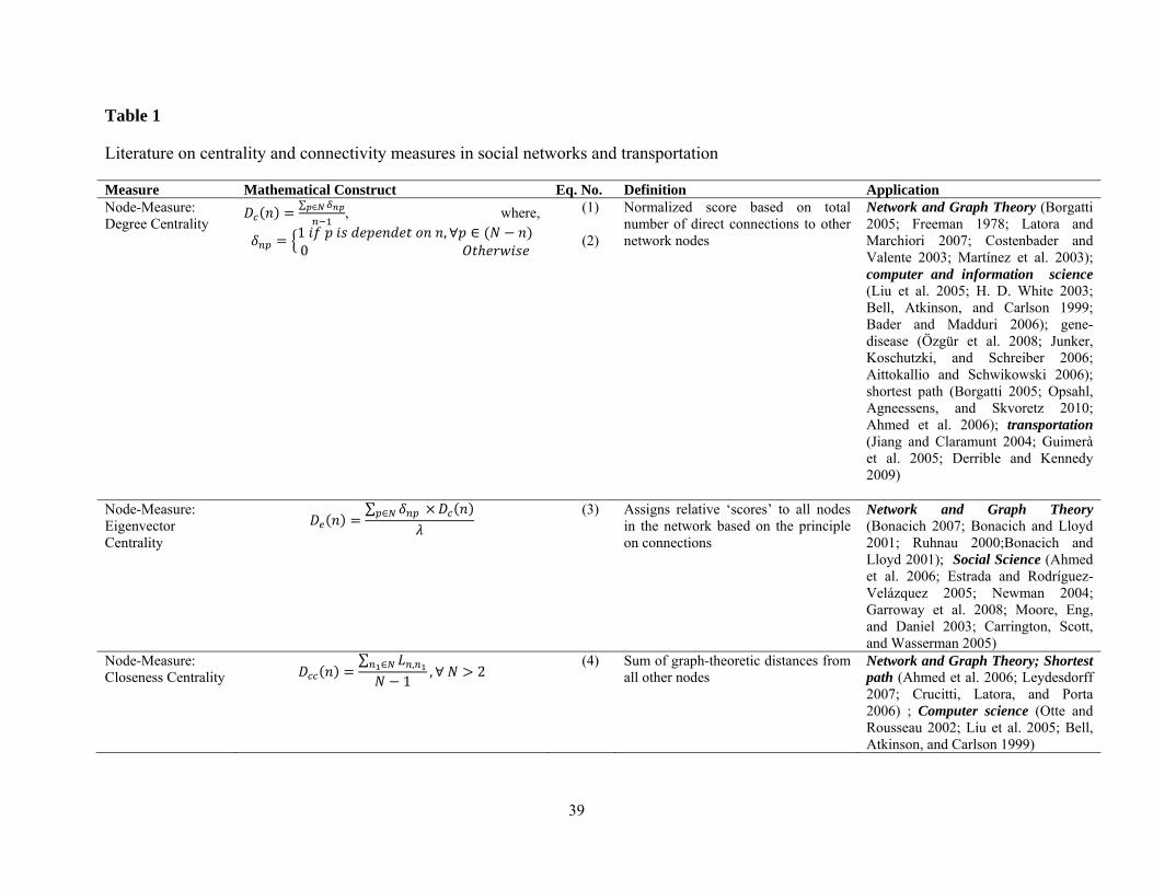
is rare. Table 1 represents a summary of connectivity index measures (or derivatives thereof)

found in the literature. The first measure in Table 1 is degree of centrality. The total number of

direct connections a node has to other system nodes is defined as the degree centrality. Equation

(1) suggest that the degree of centrality of a node in a larger network “N” is the sum of

the number of links originated from “p” number of nodes crosses through node “n” ( ), where

p represents all nodes except n (i.e. ∈ ). This measure is then normalized by dividing

by the total number of system nodes N minus 1. Equation (2) represents a conditional statement

 

6  

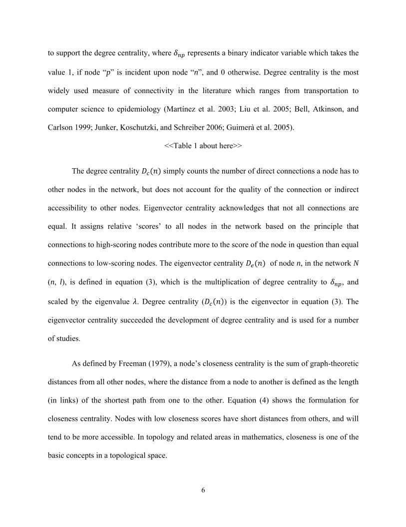
to support the degree centrality, where represents a binary indicator variable which takes the

value 1, if node “p” is incident upon node “n”, and 0 otherwise. Degree centrality is the most

widely used measure of connectivity in the literature which ranges from transportation to

computer science to epidemiology (Martínez et al. 2003; Liu et al. 2005; Bell, Atkinson, and

Carlson 1999; Junker, Koschutzki, and Schreiber 2006; Guimerà et al. 2005). 

<<Table 1 about here>>

The degree centrality simply counts the number of direct connections a node has to

other nodes in the network, but does not account for the quality of the connection or indirect

accessibility to other nodes. Eigenvector centrality acknowledges that not all connections are

equal. It assigns relative ‘scores’ to all nodes in the network based on the principle that

connections to high-scoring nodes contribute more to the score of the node in question than equal

connections to low-scoring nodes. The eigenvector centrality of node n, in the network N

(n, l), is defined in equation (3), which is the multiplication of degree centrality to , and

scaled by the eigenvalue . Degree centrality ( ) is the eigenvector in equation (3). The

eigenvector centrality succeeded the development of degree centrality and is used for a number

of studies.

As defined by Freeman (1979), a node’s closeness centrality is the sum of graph-theoretic

distances from all other nodes, where the distance from a node to another is defined as the length

(in links) of the shortest path from one to the other. Equation (4) shows the formulation for

closeness centrality. Nodes with low closeness scores have short distances from others, and will

tend to be more accessible. In topology and related areas in mathematics, closeness is one of the

basic concepts in a topological space.

 

7  

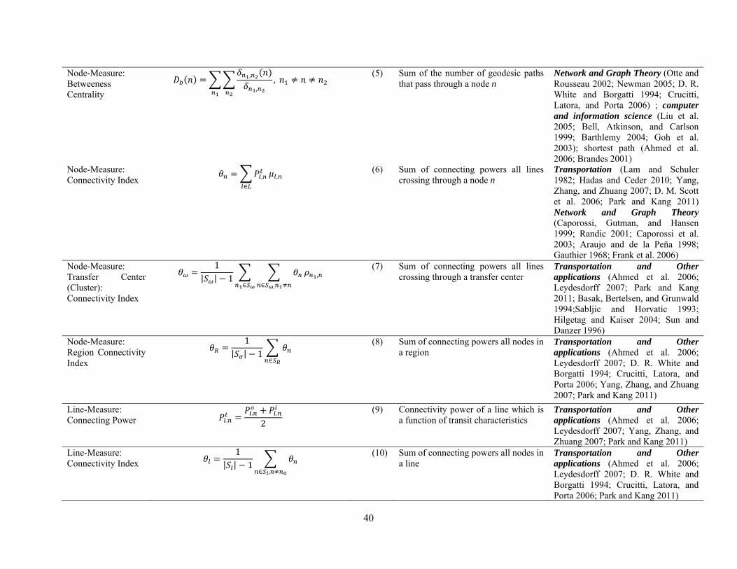
Betweenness centrality is defined as the share of times that a node n1 needs a node n

(whose centrality is being measured) in order to reach a node n2 via the shortest path. Equation

(5) shows the formulation for betweenness centrality. Alternatively, betweenness centrality

basically counts the number of geodesic paths that pass through a node n. The denominator exists

to address the case where there are multiple geodesics between n1 and n2, and node n is only

along some of them. Hence, betweenness is essentially n’s share of all paths between pairs that

utilize node n—the exclusivity of n’s position.

Previous node indexes did not take into account transit characteristics. Park and Kang

(2011) introduced the transit characteristics into the node centrality measures and proposed the

connectivity index as a true measure of a transit node. The connectivity index of a node can be

defined as the sum of connecting powers2 of all lines crossing through a node n. The connectivity

index is shown in equation (6). The total connecting power of a node is the multiple of

connecting power of a line at node n ( . ). The conditional value of presence of a line is

represented by a binary indicator variable ( , ), which takes the value 1 if line l contributes to

the connectivity at node n, and 0 otherwise. The characteristics of a link contain the performance

of a series of nodes in that link. A link is a part of the transit route, which in turn is a function of

the speed, distance, frequency, headway, capacity, acceleration, deceleration, and other factors.

Since a route will contain both in-bound and out-bound, the line performance will in part depend

upon the directionality of the transit route, that is, whether the line is circular or bidirectional.

The total connecting power of line l at node n is the average of outbound and inbound

connecting power and can be defined as

                                                            2 Please refer to equation (9) in Table 1 for the formulation of connecting power.

 

8  

,

, ,

2

(6.1)

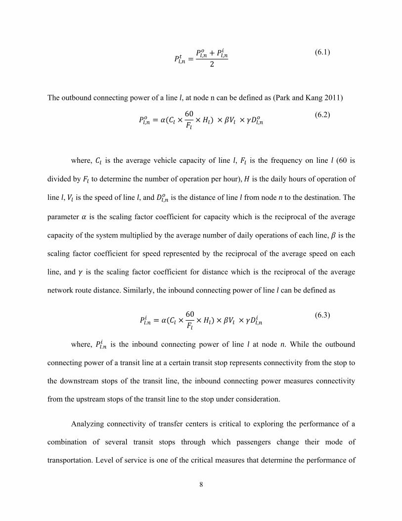
The outbound connecting power of a line l, at node n can be defined as (Park and Kang 2011)

,

60,

(6.2)

where, is the average vehicle capacity of line l, is the frequency on line l (60 is

divided by to determine the number of operation per hour), is the daily hours of operation of

line l, is the speed of line l, and , is the distance of line l from node n to the destination. The

parameter is the scaling factor coefficient for capacity which is the reciprocal of the average

capacity of the system multiplied by the average number of daily operations of each line, is the

scaling factor coefficient for speed represented by the reciprocal of the average speed on each

line, and is the scaling factor coefficient for distance which is the reciprocal of the average

network route distance. Similarly, the inbound connecting power of line l can be defined as

.

60,

(6.3)

where, . is the inbound connecting power of line l at node n. While the outbound

connecting power of a transit line at a certain transit stop represents connectivity from the stop to

the downstream stops of the transit line, the inbound connecting power measures connectivity

from the upstream stops of the transit line to the stop under consideration.

Analyzing connectivity of transfer centers is critical to exploring the performance of a

combination of several transit stops through which passengers change their mode of

transportation. Level of service is one of the critical measures that determine the performance of

 

9  

the transfer center. Equation (7) represents the connectivity index of a transfer center. Where,

, is the passenger acceptance rate and is defined as

,,

(7.1)

where, a and b are the parameters of passenger acceptance rate, and , is the transfer time to

travel from node n1 to n. The parameters for a and b are assumed from Kim and Kwon (2005)

and estimated based on model estimation which found that walk time provided an R-square value

of .9846; that is, walk time alone explained 98.46 percent of the passenger transfer acceptance

rates.

Similarly, the connectivity index of a region (equation 8) can be defined as the sum of

connectivity indexes of all nodes and scaled by the density measure, where is a density

measure of region R. The density could be a measure in population, employment, and household

in the region. The line connecting power and connectivity indexes are shown in equation (9), and

(10).

3. Problem Statement and Objectives

Many measures of transit service and accessibility have been put forth in the literature, but few

offer a metric to measure the quality of service and performance of a large multi-modal regional

transit system. The literature that does purport to offer such insight requires significant amounts

of data not only about the transit system, but also of the complete demographics of the service

area (Beimborn et al. 2004, Modarres 2003). Other methods require a full transportation demand

and transit assignment models, tools that are prohibitively expensive for many localities (Lam

and Schuler 1982).

 

10  

Measuring transit system performance and the level of service at many different levels is

vital to funding decisions (Dajani and Gilbert 1978). Agencies with the objective to improve the

transit system using external funds must make the case that the project will be a worthwhile

improvement to the system. At the same time, agencies interested in investigating the potential

effect of removing a stop, group of stops or transit line from service must know the potential

effect it will have on the performance of the system. In the absence of complex transportation

demand models, this information is nearly impossible to obtain (Baughan et al. 2009). A

methodology that reduces the need for large amounts of data, yet provides important information

on system performance is critical to the decision making process. Transit planning agencies may

also be interested in applying such an index to determine the best use of land surrounding well

connected transit nodes. Beyond Transit Oriented Development (TOD) style plans, the

connectivity index provides a way for planners to measure passenger acceptance rates and

accessibility for a single node based on its access within an entire multi-modal regional

transportation network.

The objectives of this paper are several fold, with the overall goal of providing a strong

measure of system performance with the lowest possible data requirements. This paper will first

seek to construct a list of node and link based commonly encountered flow processes and define

them in terms of a few underlying characteristics; second, to determine and propose the best

suited measures in terms of transit connectivity; third, to examine these measures by running

simulations of flow processes and comparing the results in a real world case study; and fourth, to

suggest the best practices which can be adopted for decision making. All the aforementioned

problems require the development of a tool to quantify connectivity of a public transportation

 

11  

system. The proposed methodology is presented in the next section and the notations are shown

in Appendix-I.

4. Methodology

The methodology presented in this paper is for transit systems at different levels. As the very

nature of nodes, lines, transfer centers and regions, each require a unique formulation. The

description below explains the mathematical construct of these transit levels in a step-by-step

manner.

4.1 Node Connectivity The proposed methodology consists of better representations of transit node index measures. In

the proposed formulation we consider the congestion effects achieved because of lane sharing of

transit lines of buses, light rail, bus rapid transit, and other similar transit facilities. We have

redefined the connecting power of a transit line. The other measures have not incorporated the

transit attractiveness as it relates to land use and transportation characteristics of the area the

associated with the transit line. As discussed previously, the connecting power of a transit line is

a function of the inbound and outbound powers, as the connecting power may vary depending on

the direction of travel. The inbound and outbound connecting power of a transit line can be

redefined as follows.

, , ,

(11)

, , ,

(12)

The addition in equation (11) is a term for activity density of transit line "l" at node "n",

and is the scaling factor for the variable. The density measurement represents the development

pattern based on both land use and transportation characteristics. The literature defines the level

 

12  

of development a number of ways, but for simplification purposes we have considered it to be

the ratio of households and employment in a zone to the unit area. Mathematically, activity

density (equation (13)) is defined as:

,

, ,

Θ ,

(13)

The connectivity index measures aggregate connecting power of all lines that are accessible to a

given node. However not all lines are equal; nodes with access to many low quality routes may

attain a connectivity index score equal to a node with only a couple very high quality transit

lines. This means that while both nodes are able to provide good access, the node with the fewest

lines provides the most access with the lowest need to transfer. To scale the index scores based

on the quality of individual lines, that is, scaling for the least number of transfers needed to reach

the highest number and quality of destinations, the node scores are adjusted by the number of

transit lines incident upon the node. The inbound and outbound connecting power of a transit line

can be further refined as:

, , , ,

(14)

, , , ,

(15)

This equation adds the number to transit lines “l” at node “n”, and is the scaling factor for the

number of transit lines. The transfer scale is simply the sum of the connectivity index scores for

each of the transit lines that cross a node divided by the count of the number of lines that are

incident upon the node. The transfer scaled index (equation (13)) is defined as:

,∑ ,

Θ

(16)

 

13  

4.2 Line Connectivity The total connecting power of a line is the sum of the averages of inbound and outbound

connecting powers for all transit nodes on the line as presented in equation (6.1) scaled by the

number of stops on each line. The scaling measure is used to reduce the connecting score of lines

with many stops like bus lines to properly compare to lines with only a few stops like rail. The

line connectivity can be defined as following:

| | 1 ,

(17)

4.3 Transfer Center The concept of a connectivity index of a transfer center is different from the connectivity

measure of a conventional node. Transfer centers are groups of nodes that are defined by the ease

of transfer between transit lines and modes based on a coordinated schedule of connections at a

single node or the availability of connections at a group of nodes within a given distance or walk

time. This paper defines a transfer center as the group of nodes within half mile of any rail

station in the transit network. The sum of the connecting power of each node in the transfer

center is scaled by the number of nodes on the transfer center. Thus, a node in a heavily dense

area is made comparable to the transfer center in a less dense area. This scaling procedure is

particularly important when comparing transfer centers in a multimodal network where one

transfer center may be primarily served by a well-connected commuter rail line and other may

have many bus lines and rail lines connecting to the center. The following equation shows the

connectivity index of a transfer center.

| | 1 . , (18)

 

14  

4.4 Regional (large area) Connectivity The connecting power of a Region or any other large area has several important implications.

The performance of a given area is the sum of the connectivity of all nodes within that area

scaled by the number of nodes. This scaling makes it possible to compare the quality of

connectivity between areas of differing density. The regional connectivity index equation is

shown below.

| | 1 ,

(19)

5. Example Problem

In this section, the methodology is described with the help of an example problem. The example

network shown in Fig. 1(a) consists of (1) ten stops, (2) five lines, (3) two transfer centers, and

(4) five Traffic Analysis Zones (TAZs). Three characteristics of each line such as operating

speed, capacity and number of operations are given. Each TAZ is attributed with a density

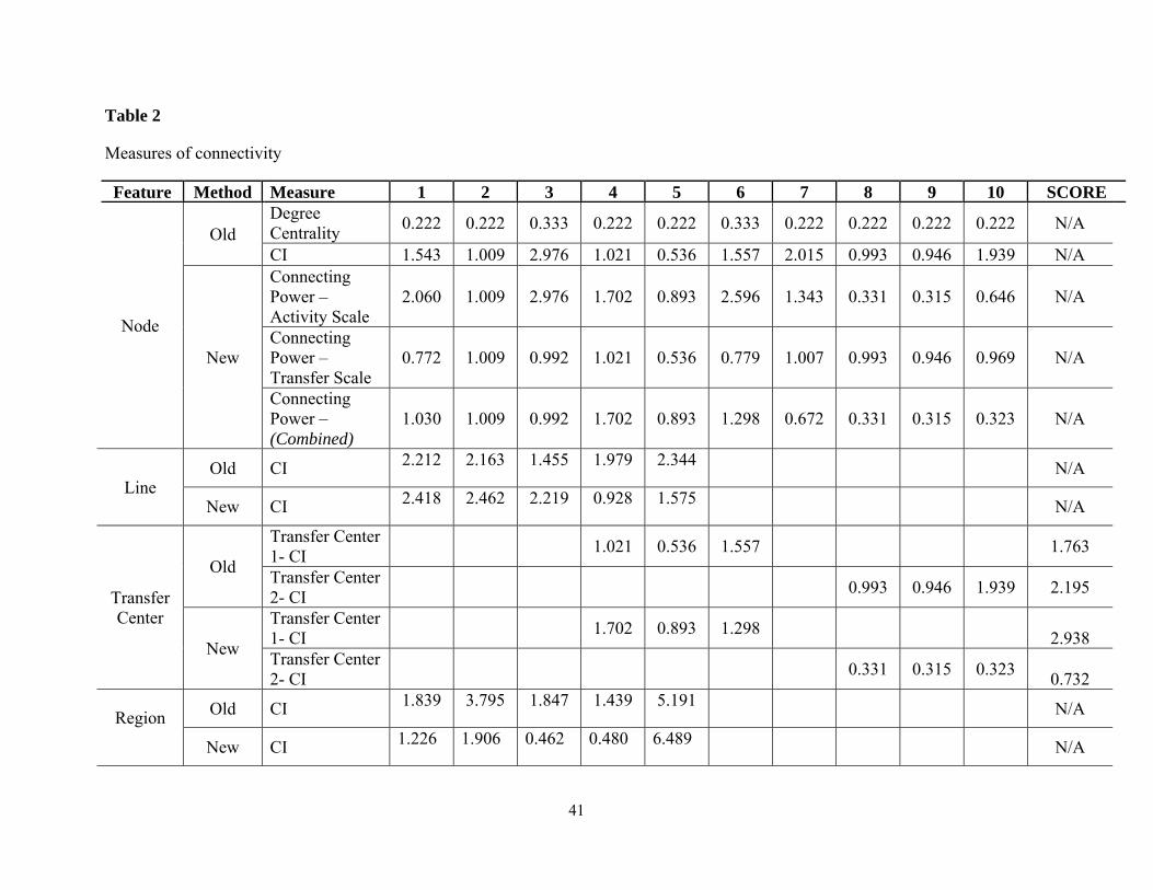
measure which is the ratio between the population and corresponding area. Table 2 shows the

comparison of the approaches reported in the literature, and the new approach, at the node, line,

transfer center, and region level. In the comparison only degree centrality is obtained from the

literature, which is presented at the node level. For the line, node and transfer center

connectivity, the related measures from the literature are analyzed in the example problem.

<<Fig. 1(a) about here>>

<<Fig. 1(b) about here>>

 

15  

5.1 Node and Line Level The node level measures are presented in Table 2. Degree centrality of node-1 is 0.222 (i.e. 2/9),

as there are two nodes incident upon node-1 (node 2, and node 5), and there are nine remaining

nodes in the system (please refer to equation (1) for the formula). Similarly degree centrality for

all the nodes can be determined. The connectivity index of node-1 is 1.543. This number is

derived from three steps:

<<Table 2 about here>>

A zoomed version of node-1 is shown in Fig. 1(b). There are two lines crossing through node-1

(Line-1 and Line-3). The inbound connecting power of line-1 at node-1 ( . ) is calculated from

equation 6.2. ,

. .400

.20

.10 =1.008

where, = 468.457, =20.062, and = 8.437. The capacity of line-1 is 400 (i.e. 8x50). These

parameters represent the average of all the corresponding characteristics. Similarly, the outbound

connecting power of line-1 at node-1 ( . ) is 1.008. So the total connecting power of line-1 at

node-1 ( . ) is 1.008 (i.e. (1.008+1.008)/2).

The inbound connecting power of line-3 at node-1 is

. .500

.17

.5 = 0.535

The outbound connecting power ( . ) of line-3 at node-1 is 0.535, and the total connecting

power ( . ; is the average of inbound and outbound connecting powers, i.e. (0.535+0.535)/2 =

0.535.

The connectivity index of node 1 is

. . . 1.008 0.535 1.543

 

16  

Similarly the connecting powers of all the nodes can be determined.

Now the connecting power can be further improved using the extended the methodology.

Please see equation (11), and (12) for formulation on connecting power for nodes. The inbound

connecting power of line-1 at node-1 using activity scale can be determined as the ratio of

density of node 1, which resides in TAZ-1 (density =4), and the average system density

(density=3). Alternatively, 1.008*(4/3) = 1.344. Similarly the outbound connecting power for

line-1 at node-1 is 1.344. The total connecting power of line-1 at node-1 is the sum of inbound

and outbound connecting powers, i.e. 1.344. The inbound, outbound, and total connecting power

of line-3 at node-1 is 0.535*(4/3) = 0.714. So the total connecting power of node-1 using activity

scaling is 1.344+0.714=2.060. It should be noted that the connecting power of node-1 has

increased from 1.543 (without using activity scaling) to 2.060 with using activity scaling.

Following similar convention, the connecting power using transfer scale can be used. The

connecting power is related to the incidence of lines passing through a node. Please see equation

(14), (15), and (16) for formulation on connecting power for nodes. There are two transit lines

crossing through node-1. So the connecting power using transfer center scale for node-1 is

1.545/2, i.e. 0.772. The next step is to determine the combined connectivity index using both

activity scale and transfer scale. For node-1 the revised connectivity index of node 1 is 2.060/2 =

1.030. Similarly connectivity indexes for all nodes can be determined.

5.2 Transfer Center Level There are two transfer centers in the example problem (Fig. 1 (a)). Transfer center-1 connects

through three nodes (4, 5, and 6). The connectivity index of these three nodes using the old

method is 1.021, 0.536, and 1.557. The connectivity index of the transfer center-1 is 1.763, i.e.

(1.021+0.536+1.557) / (3-1). But with the proposed method, the connectivity index of transfer

 

17  

center-1 is 2.938, i.e. (1.702+0.893+1.298) / (3-1). Similarly the connectivity index of transfer

center-2 is 2.195 and 0.732 using the extended and existing methods respectively. The difference

in the score of the transfer centers is the deference in the access each stop theoretically provides.

Node 6 is in a dense area with many activities and node 10 is in a rural location with few

activities; thus method two provides a measure of how well connected a center is to the system

and to the underlying area that creates demand for transit trips.

5.3 Region Level There are five zones (or regions) in the example problem. The connectivity of each zone is the

sum of the connectivity index for all nodes in the zone scaled by the population of the zone

relative to average zonal population. Zone-1 contains one node (1) and a population of 25. The

connectivity of Zone-1 under the old method is 1.839 (i.e. 1.545*(25/21)); with the proposed

method the zone has a connectivity score of 2.452 (i.e. 1.030*(25/21). While the top two zones

are in the same order, there are differences between the rank of the zones and the scale of the

index for each zone. The primary difference between each zone with the proposed method is the

quality of each line in terms of the number of transfers it requires to each a given score.

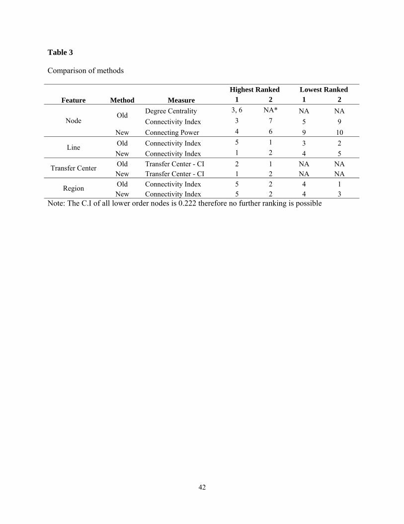
5.4 Synthesis of the Example Problem

For a comparison of the previous and proposed transit network measures, a summary of the

results is shown in Table 3.

<<Table 3 about here>>

The degree of centrality is a simple method that provides only an indication of the best

connected nodes in the simplest of terms, the normalized number of connections, but goes no

further. The existing connectivity index attempts to refine the centrality measure by including

transit characteristics but fails to account for productions, attractions and required transfers that

 

18  

can alter the real connectivity of a system. The extended method adds context to the existing

method by scaling for the opportunities in area surrounding the node and the number of transfers

required to get to those opportunities.

Under the existing connectivity index method node-3, just as with degree centrality, is the

highest ranked node; this is because the sum of the characteristics of all the lines connecting to

the node is higher than all other nodes. Under the extended connecting power method, the

connecting power of each line is scaled by the activity density and normalized by the number of

lines (or transfers). As a result, node-4 which is situated in a high density location, close to other

high density nodes and incident upon a single line with the highest connecting power is the top

ranked node.

The existing and extended methodologies of transfer centers come to opposite conclusions about

transfer center rankings. While both account for the quality of service at each center, that is,

route speed, capacity and operations, the connecting power method prioritizes transfer center-1

due to the density of its location and level of connection it has to other high quality areas. It

ranks transfer center-2 lower because the transfer center nodes are in low density areas and the

connecting lines provide direct connections only to relatively low quality nodes.

6. Case Study

The proposed framework is applied to a comprehensive transit network in the Washington-

Baltimore region. The complete transit network is adapted from Maryland State Highway

Administration data. The transit database consists of two largest transit systems namely,

Washington Metropolitan Area Transit Authority (WMATA), and Maryland Transit

Administration (MTA). WMATA is a tri-jurisdictional government agency that operates transit

 

19  

service in the Washington, D.C. metropolitan area, including the Metrorail (rapid transit),

Metrobus (fixed bus route) and MetroAccess (paratransit), and is jointly funded by the District of

Columbia, together with jurisdictions in suburban Maryland and northern Virginia. There is

approximately $300 million spent in the WMATA capital, operating and maintenance cost of

which $150 million per year of Federal funds available that are required to be matched by $50

million in annual contributions from DC, Northern Virginia and suburban Maryland, each for ten

years.

WMATA has the second highest rail ridership in the US with over 950,000 passengers

per day. This is second only to New York. The WMATA Metro provides an extensive heavy rail

system with 106.3 route miles. The WMATA bus system also serves an extensive ridership of

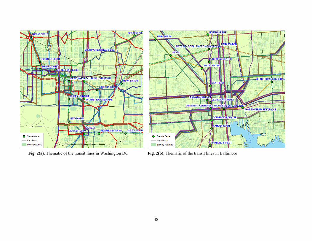
over 418,000 unlinked daily trips. Fig. 2(a) shows the WMATA network at Union Station.

<<Fig. 2(a) about here>>

<<Fig. 2(b) about here>>

On the other hand, MTA is a state-operated mass transit administration in Maryland.

MTA operates a comprehensive transit system throughout the Baltimore-Washington

Metropolitan Area. There are 77 bus lines serving Baltimore's public transportation needs. The

system has a daily ridership of nearly 300,000 passengers along with other services that include

the Light Rail, Metro Subway, and MARC Train. The Baltimore Metro subway is the 11th most

heavily used system in the US with nearly 56,000 daily riders. Nearly half the population of

Baltimore lack access to a car, thus the MTA is an important part of the regional transit picture.

The system has many connections to other transit agencies of Central Maryland: WMATA,

Charm City Circulator, Howard Transit, Connect-A-Ride, Annapolis Transit, Rabbit Transit,

 

20  

Ride-On, and TransIT. Fig. 2(b) shows MTA network around Camden in station downtown

Baltimore. Both the WMATA Metro rail system and the Baltimore transit system are connected

by the MARC commuter rail system. This system has a daily ridership of over 31,000. In the

next section, results of the proposed methodology are discussed (APTA 2011). The complete

methodology is integrated in a Geographic Information System (GIS) user interface using

ArcInfo (ESRI 2010).

7. Results

The results reported in the following sections are based on the application of methods developed

in this paper on a large-scale multi-modal network of Washington DC and Baltimore region.

Table 4 provides a summary of Baltimore/Washington regional transit system. The system

represents one of the largest and most heavily patronized transit systems in the county. The

application of the methodology to this complex network provides a demonstration of public

transit performance in the Baltimore/Washington Region.

<<Table 4 about here>>

7.1Nodelevel

The Washington/Baltimore region has a significant number of transit nodes, each of which

provide a varying degree of connectivity to the network. Determining network connectivity and

funding prioritization is a highly complex task in a multi-modal network. Funding prioritization

is additionally aided by the connectivity index by providing decision makers with a tool to

measure network resilience. As with any network, transit systems are designed to interact with

many different nodes, while remaining functional in the event that a particular node becomes

 

21  

inaccessible. Additionally, resiliency tests based on connectivity can reveal if there is an over

concentration of connections which rely on a given node, line, or region.  

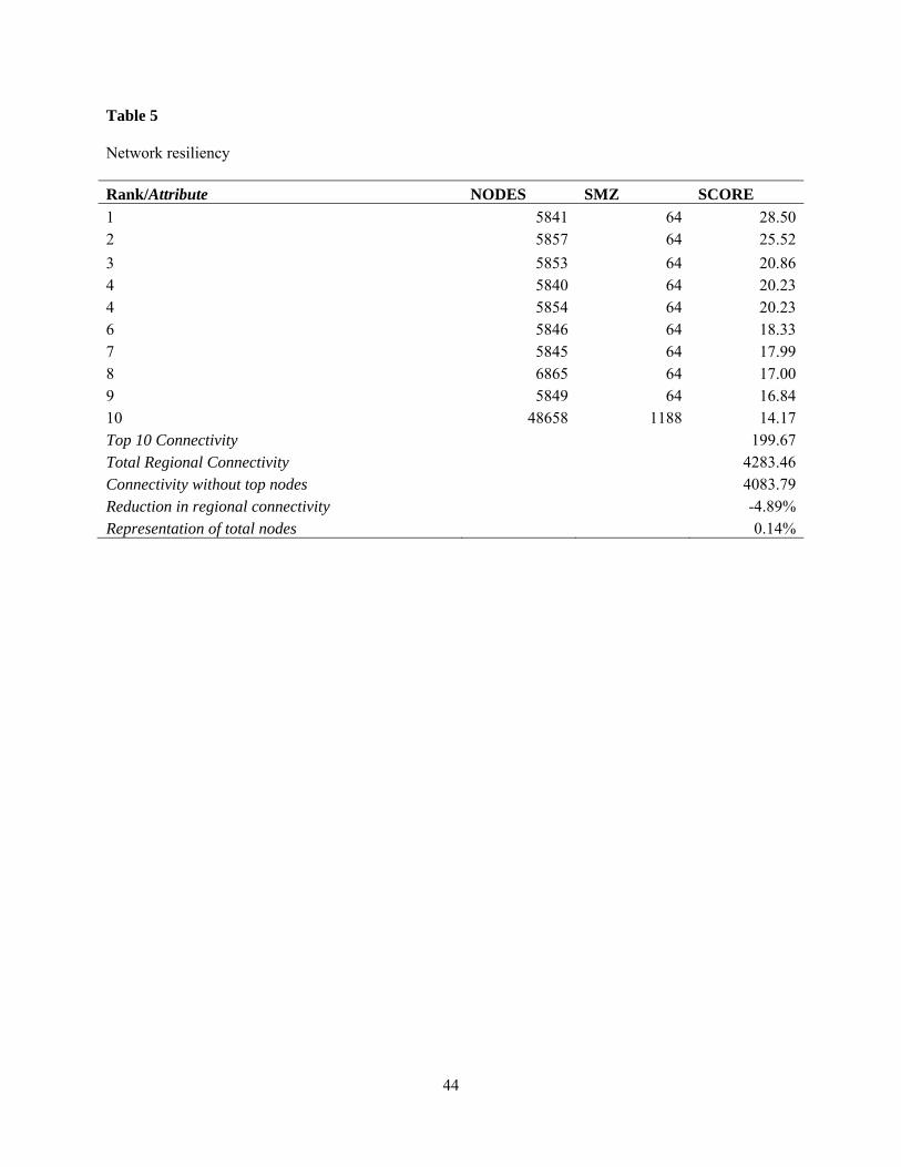
<<Table 5 about here>>

Table 5 shows the top ten nodes in the network. This table presents a potential problem for the

regional transportation network. The results show that nine of the ten most connected nodes are

located in the same zone. These zones are less than a few blocks from each other, thus it is

feasible that an event could occur that would remove these nodes from service. If all ten of the

nodes were to be removed from service, regional network connectivity would be reduced from a

score of 4,283 to 4,083 or by about 5%. This is remarkable in that these nodes represent less than

5% of connectivity and less than 0.1% of the total system nodes, yet the system connectivity is

heavily reliant of these few connections. A similar comparison can be made for all the nodes in

the network.

Fig. 3 is a three-dimensional graph of node connectivity in the Baltimore/Washington

region. The map shows the extent of connectivity for the three major transit areas, Washington

DC, Baltimore and Silver Spring. The figure also illustrates the location of zone 64 which has the

highest concentration of well-connected transit nodes.

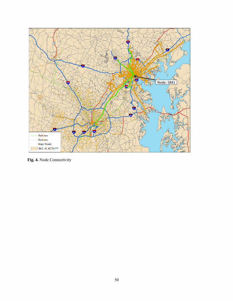
<<Fig. 4 about here>>

Fig. 4 plots the lines (rail in green and bus in orange) that the best connected node (node

number 5841 and zone number 64) in the region can reach within a single transfer. While other

nodes in the system provide access to as many locations and lines as possible, this node is able to

move riders from the origin to all of the locations shown in Fig. 4 with the fewest resources and

lowest transfer times. Additionally, a review of this site shows that land use can be improved to

 

22  

capitalize on the regional connectivity of this node. To the north of the node is the Baltimore

City Hall and the US Post Office and Court house. To the south of the node is a parking structure

and a surface parking lot. Since this node can be reached from most of Baltimore in a single

transfer and much of Washington DC in two transfers, the city could opt to zone the area for

higher density and encourage development. This would likely not significantly increase

congestion around the site if transit usage could be encouraged.

7.2LineLevelThe quality of connectivity for a transit line is determined by several factors. First the line needs

to provide access to at least some dense development, second the line should provide access to

desirable locations with the fewest number of transfers; third the line must connect to other

modes to maximize connectivity. The line connectivity index is applied to the

Baltimore/Washington regional transportation network. The region provides both rail and bus

services. The rail services analyzed in this paper include WMATA’s Metro, Baltimore’s light

rail, metro system and the regional MARC commuter lines jointly operated by AMTRAK and

CSX. All significant local and regional bus services were included in the analysis. Not included

in the study were national bus and rail services like Greyhound and AMTRAK. While these

services do provide a level of connectivity, the primary concern of this paper is how local and

regional systems work to create regional connectivity that local and state decision makers can

influence.

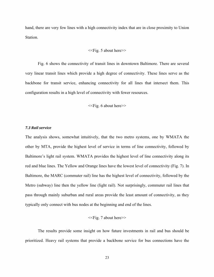
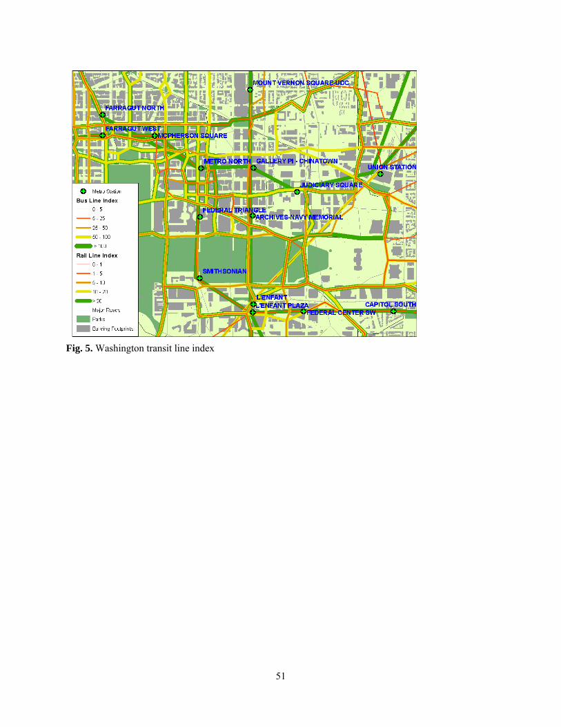
Fig. 5 shows the line connectivity index for the federal triangle area and vicinity of

Washington DC. The map clearly shows that there is a concentration of highly connected lines

that are near the Farragut, McPherson Square and Metro North transfer centers. On the other

 

23  

hand, there are very few lines with a high connectivity index that are in close proximity to Union

Station.

<<Fig. 5 about here>>

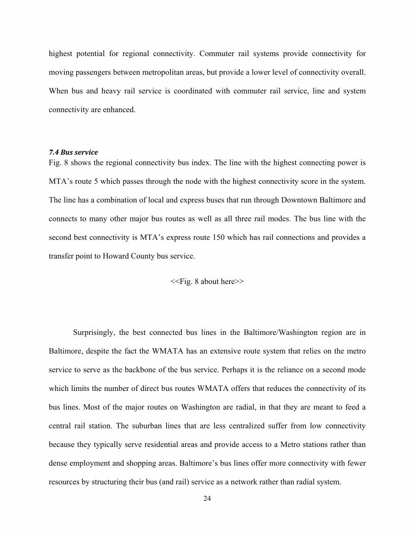
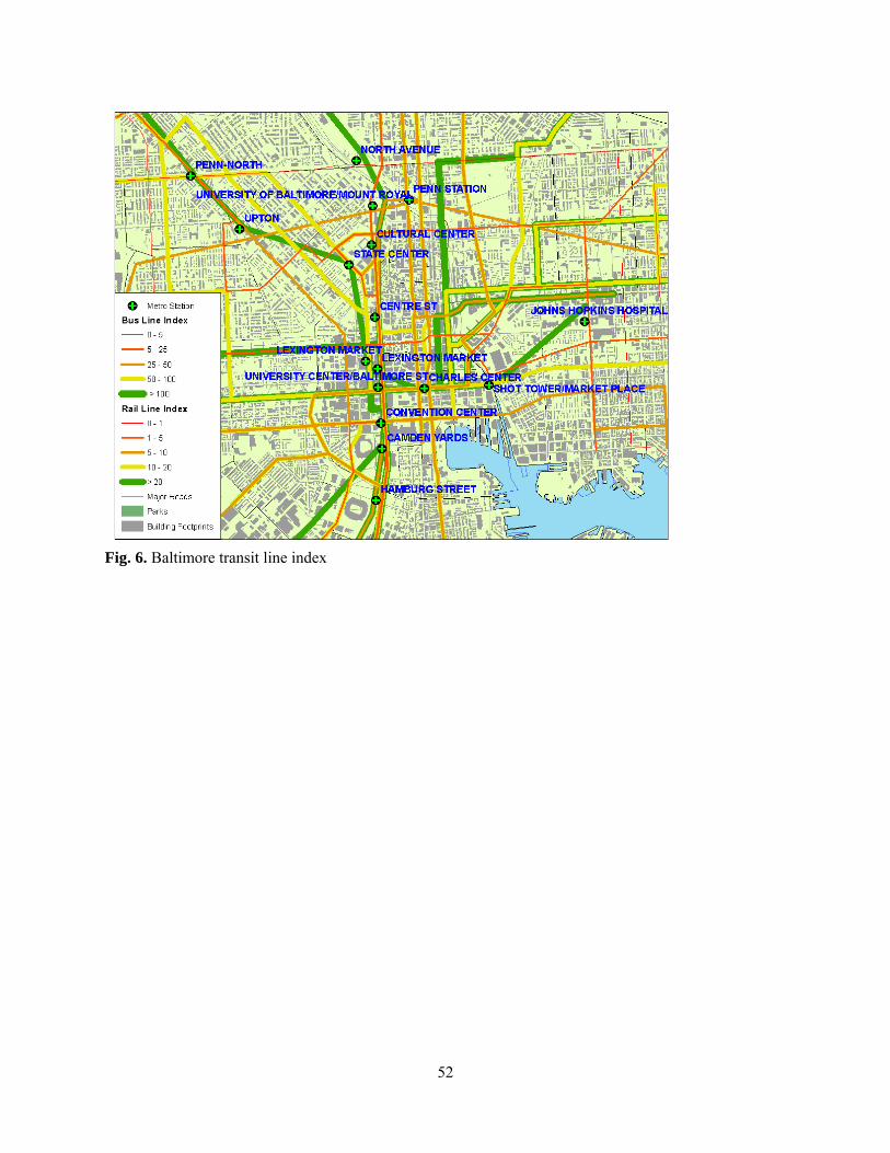
Fig. 6 shows the connectivity of transit lines in downtown Baltimore. There are several

very linear transit lines which provide a high degree of connectivity. These lines serve as the

backbone for transit service, enhancing connectivity for all lines that intersect them. This

configuration results in a high level of connectivity with fewer resources.

<<Fig. 6 about here>>

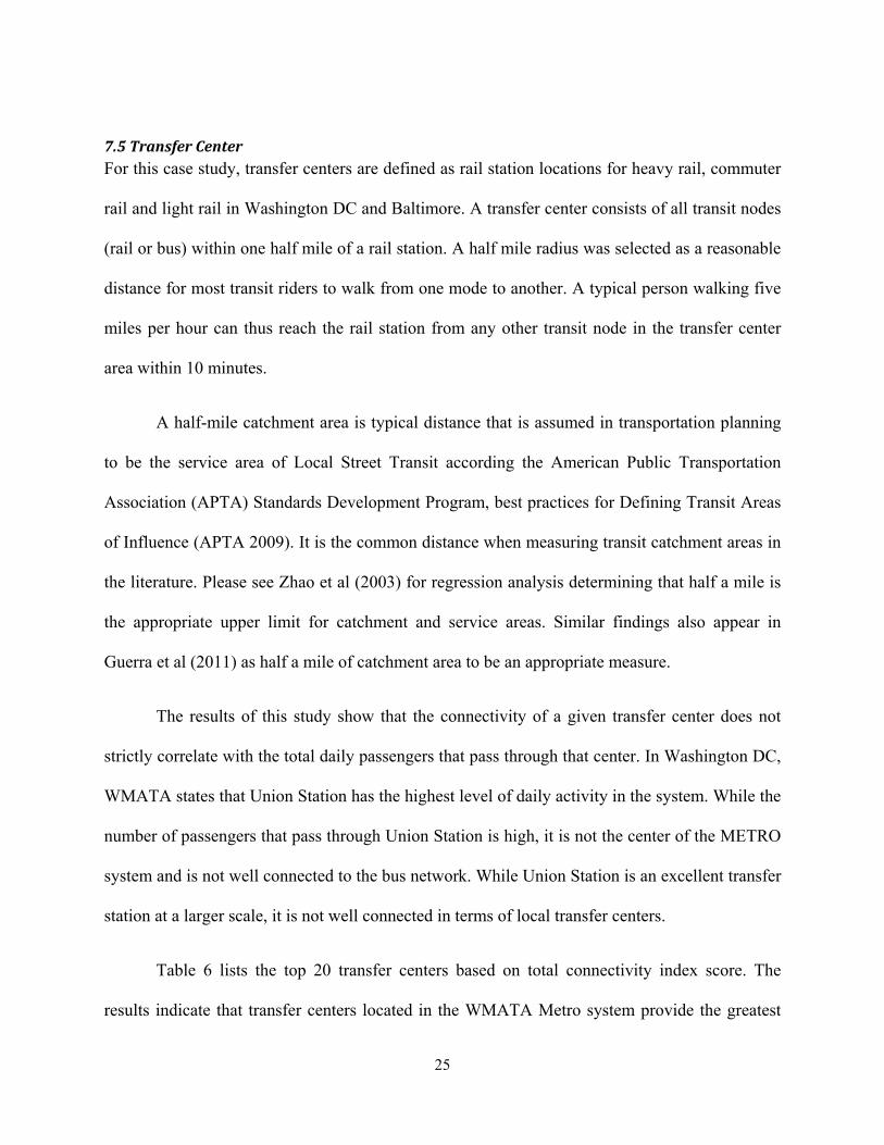
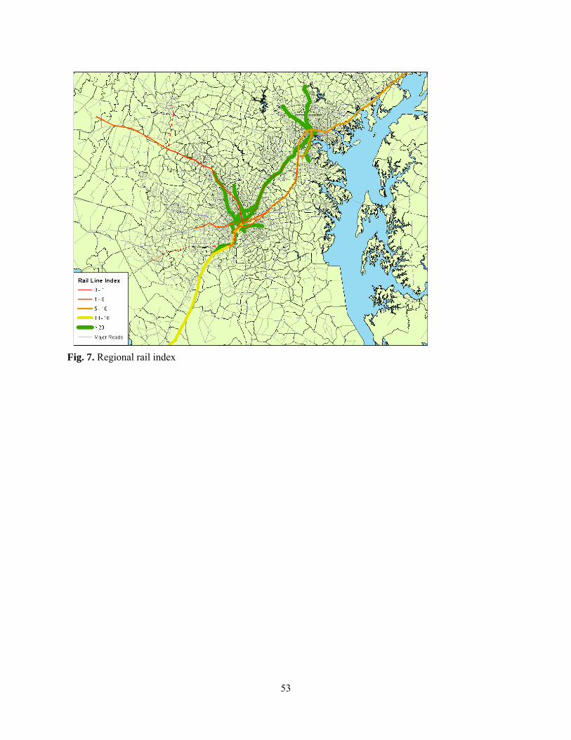
7.3Railservice

The analysis shows, somewhat intuitively, that the two metro systems, one by WMATA the

other by MTA, provide the highest level of service in terms of line connectivity, followed by

Baltimore’s light rail system. WMATA provides the highest level of line connectivity along its

red and blue lines. The Yellow and Orange lines have the lowest level of connectivity (Fig. 7). In

Baltimore, the MARC (commuter rail) line has the highest level of connectivity, followed by the

Metro (subway) line then the yellow line (light rail). Not surprisingly, commuter rail lines that

pass through mainly suburban and rural areas provide the least amount of connectivity, as they

typically only connect with bus nodes at the beginning and end of the lines.

<<Fig. 7 about here>>

The results provide some insight on how future investments in rail and bus should be

prioritized. Heavy rail systems that provide a backbone service for bus connections have the

 

24  

highest potential for regional connectivity. Commuter rail systems provide connectivity for

moving passengers between metropolitan areas, but provide a lower level of connectivity overall.

When bus and heavy rail service is coordinated with commuter rail service, line and system

connectivity are enhanced.

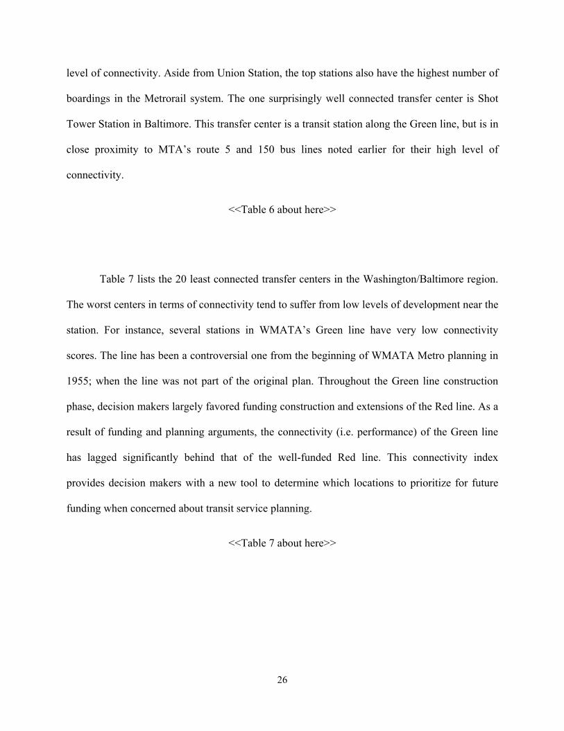
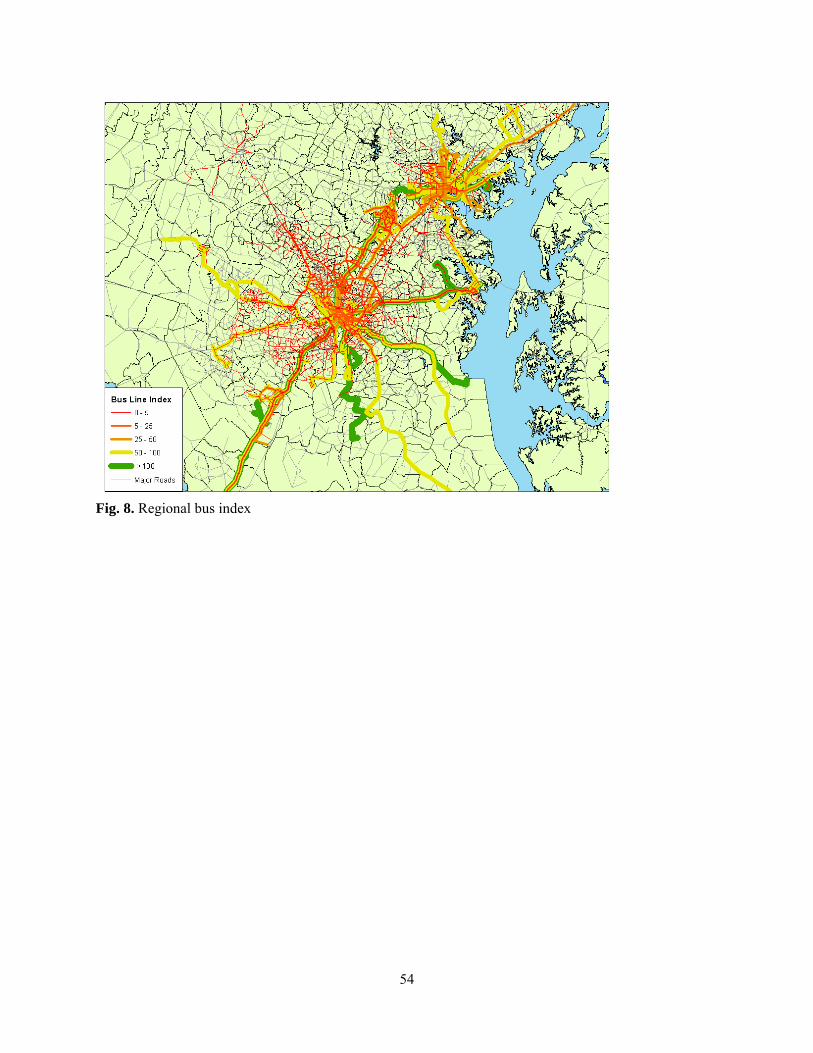
7.4BusserviceFig. 8 shows the regional connectivity bus index. The line with the highest connecting power is

MTA’s route 5 which passes through the node with the highest connectivity score in the system.

The line has a combination of local and express buses that run through Downtown Baltimore and

connects to many other major bus routes as well as all three rail modes. The bus line with the

second best connectivity is MTA’s express route 150 which has rail connections and provides a

transfer point to Howard County bus service.

<<Fig. 8 about here>>

Surprisingly, the best connected bus lines in the Baltimore/Washington region are in

Baltimore, despite the fact the WMATA has an extensive route system that relies on the metro

service to serve as the backbone of the bus service. Perhaps it is the reliance on a second mode

which limits the number of direct bus routes WMATA offers that reduces the connectivity of its

bus lines. Most of the major routes on Washington are radial, in that they are meant to feed a

central rail station. The suburban lines that are less centralized suffer from low connectivity

because they typically serve residential areas and provide access to a Metro stations rather than

dense employment and shopping areas. Baltimore’s bus lines offer more connectivity with fewer

resources by structuring their bus (and rail) service as a network rather than radial system.

 

25  

7.5TransferCenterFor this case study, transfer centers are defined as rail station locations for heavy rail, commuter

rail and light rail in Washington DC and Baltimore. A transfer center consists of all transit nodes

(rail or bus) within one half mile of a rail station. A half mile radius was selected as a reasonable

distance for most transit riders to walk from one mode to another. A typical person walking five

miles per hour can thus reach the rail station from any other transit node in the transfer center

area within 10 minutes.

A half-mile catchment area is typical distance that is assumed in transportation planning

to be the service area of Local Street Transit according the American Public Transportation

Association (APTA) Standards Development Program, best practices for Defining Transit Areas

of Influence (APTA 2009). It is the common distance when measuring transit catchment areas in

the literature. Please see Zhao et al (2003) for regression analysis determining that half a mile is

the appropriate upper limit for catchment and service areas. Similar findings also appear in

Guerra et al (2011) as half a mile of catchment area to be an appropriate measure.

The results of this study show that the connectivity of a given transfer center does not

strictly correlate with the total daily passengers that pass through that center. In Washington DC,

WMATA states that Union Station has the highest level of daily activity in the system. While the

number of passengers that pass through Union Station is high, it is not the center of the METRO

system and is not well connected to the bus network. While Union Station is an excellent transfer

station at a larger scale, it is not well connected in terms of local transfer centers.

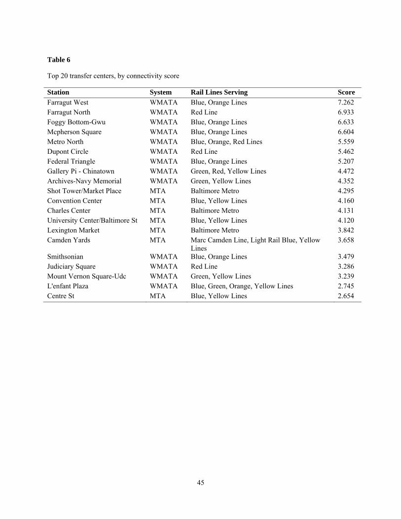
Table 6 lists the top 20 transfer centers based on total connectivity index score. The

results indicate that transfer centers located in the WMATA Metro system provide the greatest

 

26  

level of connectivity. Aside from Union Station, the top stations also have the highest number of

boardings in the Metrorail system. The one surprisingly well connected transfer center is Shot

Tower Station in Baltimore. This transfer center is a transit station along the Green line, but is in

close proximity to MTA’s route 5 and 150 bus lines noted earlier for their high level of

connectivity.

<<Table 6 about here>>

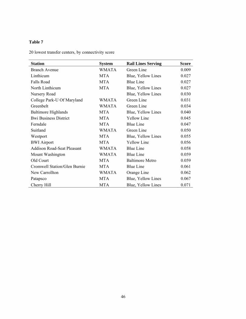
Table 7 lists the 20 least connected transfer centers in the Washington/Baltimore region.

The worst centers in terms of connectivity tend to suffer from low levels of development near the

station. For instance, several stations in WMATA’s Green line have very low connectivity

scores. The line has been a controversial one from the beginning of WMATA Metro planning in

1955; when the line was not part of the original plan. Throughout the Green line construction

phase, decision makers largely favored funding construction and extensions of the Red line. As a

result of funding and planning arguments, the connectivity (i.e. performance) of the Green line

has lagged significantly behind that of the well-funded Red line. This connectivity index

provides decision makers with a new tool to determine which locations to prioritize for future

funding when concerned about transit service planning.

<<Table 7 about here>>

 

27  

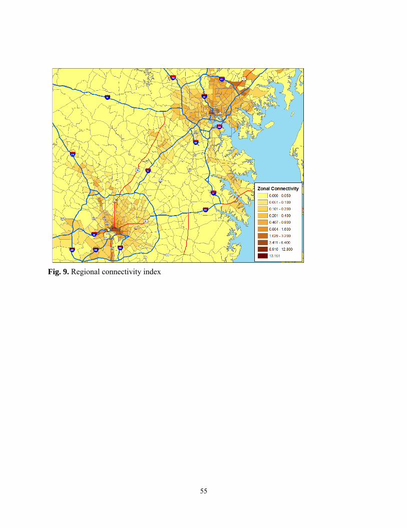
7.6Region(largeArea)

We divided the Washington/Baltimore region into 1,609 analysis zones to measure large area

connectivity. Each zone represents an aggregate of several traffic analysis zones. These zones

follow the shape of the transportation network so that no major highway is bisected by the zone

boundary. The zone structure also attempts to have an equal number of households in several

income categories and an equal amount of employment in several job types across all zones.

This level of analysis is beneficial in two ways. First, it can help to point out areas that

are under-served by transit. This can aid the prioritization of funding and other planning

activities to provide equal connectivity across the region. Secondly, the identification of highly

connected links and poorly connected links can aid in helping decision makers plan for service

that better connects lower connectivity areas with lower connectivity resources without the cost

of restructuring the system or providing new routes.

Fig. 9 shows the results of the large area connectivity analysis. It shows that zones with

rail and bus connections have the highest level of connectivity while zones that have a single rail

connection or just one bus route servicing the area have very little connectivity. In some cases a

zone has a low connectivity score even though a highly connected route passes through the zone.

These are the zones that this index is designed to capture. By simply adding an additional stop in

the area that has no other connections, yet a route running through it, residents and businesses

can have regional transit connectivity with little additional expense.

<<Fig. 9 about here>>

 

28  

8. Conclusion

The objective of this paper is to develop connectivity indicators to represent the potential ability

of a transit system encompassing comprehensive clustered development in a multimodal

transportation network. Connectivity defines the level of coordination of the transit routes,

coverage, schedule, speed, operational capacity, urban form characteristics, and is an influential

element of the image of any transit network. Though the concept of connectivity is used in social

networks and partly in transportation engineering, its application in transit analysis has been

limited. The difficulty for development of connectivity indicators lies in the complex interacting

factors embedded in a multimodal transit network encompassing various public transportation

modes with different characteristics, such as buses, express buses, subways, light rail, metro rail,

commuter and regional rail. In addition, multimodal transit networks, like road networks consist

of nodes and links. However, links in a multimodal transit network have different characteristics

from those in a road network as link in a multimodal transit network are part of a transit line that

serve a sequence of transit stops (nodes) and a stop can be served by different transit lines;

multiple links may exist between nodes in a multimodal transit network. The indicator

development process is further complicated as connectivity varies by urban form with

differences among geographical, land use, highway and trip pattern characteristics between

regions. The performance indicator should include all the aforementioned complexities and

should be quantified to portray connectivity of the multimodal transportation network.

In this paper first the connectivity indexes used for different purposes in the social

networks are reviewed. Then a new set of indicators are developed to reflect the transit mode,

network, and zonal characteristics. A set of connectivity indexes is developed for (1) node, (2)

link, (3) transfer center, and (4) region. The node connectivity index includes the transit lines

 

29  

passing through it, their characteristics such as speed, capacity, frequency, distance to

destination, activity density of the location, and degree centrality. The link connectivity index is

the sum of connectivity indexes of all stops it passes through and normalized to the number of

stops. The concept of a connectivity index of a transfer center is different from the connectivity

measure of a conventional node. Transfer centers are groups of nodes that are defined by the ease

of transfer between transit lines and modes based on a coordinated schedule of connections at a

single node or the availability of connections at a group of nodes within a given distance or walk

time. The sum of the connecting power of each node in the transfer center is scaled by the

number of nodes in the transfer center. Thus, a node in a heavily dense area is made comparable

to a transfer center located in a less dense area. Lastly, the connecting power of a region is

defined by the urban form, and the characteristics of nodes, lines, and transfer centers.

The connectivity index proposed in the paper is presented with the help of an example

network. The example problem shows the distinction between proposed extended connectivity

indexes, and existing formulations found in the literature in a step-by-step manner. The results of

the example problem identifies measures in terms of nodes located in rural areas, lines with

lower speed, lack of frequency, lower capacity, and missed transfers. The lack of transfer

between nodes that occurs in multi-legged trips is a major contributor to the calculation of the

connectivity index. The proposed methodology is also applied to a comprehensive multimodal

transit network in the Washington-Baltimore region. The network resiliency is examined at node,

link, transfer center, and regional level. Highly connected transfer centers and regions are

identified.

The major contributions of the paper include (1) extending the graph theoretic approach

to determine the performance of the multimodal transit network; (2) quantifying the measures of

 

30  

connectivity at the node, line, transfer center, and regional level; (3) applying the methodology to

demonstrate the proposed approach in a simplified example problem; (4) examining the transit

network performance of Washington-Baltimore region; (5) providing a comprehensive

framework for analyzing connectivity, and efficiency of transit networks for agencies that do not

have access to well-developed travel demand and transit assignment models, and (6) integrating

the complete methodology in a GIS user interface to enhance visualization, and interpretation of

the results. Further this study can be extended to analyze changes in the performance measure

with changes to the transit network as a sensitivity analysis; incorporating other attributes to the

current formulation, and extending the proposed research for prioritizing locations in the case of

transit emergency evacuation.

9. Acknowledgement

The authors are thankful to Dr. Seong-Cheol Kang, Associate Research Fellow at The Korea

Transport Institute, for sharing his paper and initial ideas on transit connectivity.

10. Reference

Ahmed, Adel, Tim Dwyer, Michael Forster, Xiaoyan Fu, Joshua Ho, Seok-Hee Hong, Dirk

Koschützki, et al. 2006. GEOMI: GEOmetry for Maximum Insight. In Graph Drawing,

ed. Patrick Healy and Nikola S. Nikolov, 3843:468-479. Berlin, Heidelberg: Springer

Berlin Heidelberg.

Aittokallio, Tero, and Benno Schwikowski. 2006. “Graph-based methods for analysing networks

in cell biology.” Briefings in Bioinformatics 7 (3): 243 -255. Araujo, O., and J. A. de la

 

31  

Peña. 1998. “The connectivity index of a weighted graph.” Linear Algebra and its

Applications 283 (1-3; November 1): 171-177.

APTA. 2009. Defining Transit Areas of Influence. American Public Transportation Association,

Document Number: APTA SUDS-UD-RP-001-09, available at

http://www.aptastandards.com/portals/0/SUDS/SUDSPublished/APTA%20SUDS-UD-009-

01_areas_of_infl.pdf, Accessed, February 4, 2012.

APTA. 2011. Public Transit Ridership Report, Third Quarter 2011 (www.apta.com); at

http://www.apta.com/resources/statistics/Documents/Ridership/2011-q3-ridership-APTA.pdf

Bader, David A., and Kamesh Madduri. 2006. Parallel Algorithms for Evaluating Centrality

Indices in Real-world Networks. In Parallel Processing, International Conference on,

0:539-550. Los Alamitos, CA, USA: IEEE Computer Society.

Barthlemy, M. 2004. “Betweenness centrality in large complex networks.” The European

Physical Journal B - Condensed Matter 38 (2; March): 163-168.

Basak, Subhash C., Sharon Bertelsen, and Gregory D. Grunwald. 1994. “Application of graph

theoretical parameters in quantifying molecular similarity and structure-activity

relationships.” Journal of Chemical Information and Computer Sciences 34 (2; March 1):

270-276.

 

32  

Baughan, K. J., Constantinou, C. C., and Stepanenko, A. S. (2009). “Understanding Resiliency

and Vulnerability in Transport Network Design,” Proceedings of European Transport

Conference.

Bell, David C., John S. Atkinson, and Jerry W. Carlson. 1999. “Centrality measures for disease

transmission networks.” Social Networks 21 (1; January): 1-21. Bonacich, Phillip. 2007.

“Some unique properties of eigenvector centrality.” Social Networks 29 (4; October):

555-564.

Bonacich, Phillip, and Paulette Lloyd. 2001. “Eigenvector-like measures of centrality for

asymmetric relations.” Social Networks 23 (3; July): 191-201.

Borgatti, Stephen P. 2005. “Centrality and network flow.” Social Networks 27 (1; January): 55-

71.

Brandes, Ulrik. 2001. “A faster algorithm for betweenness centrality.” The Journal of

Mathematical Sociology 25 (2; June): 163-177.

Caporossi, Gilles, Ivan Gutman, and Pierre Hansen. 1999. “Variable neighborhood search for

extremal graphs: IV: Chemical trees with extremal connectivity index.” Computers &

Chemistry 23 (5; September 1): 469-477.

Caporossi, Gilles, Ivan Gutman, Pierre Hansen, and Ljiljana Pavlovic. 2003. “Graphs with

maximum connectivity index.” Computational Biology and Chemistry 27 (1; February):

85-90.

 

33  

Carrington, Peter J., John Scott, and Stanley Wasserman. 2005. Models and methods in social

network analysis. Cambridge University Press.

Costenbader, Elizabeth, and Thomas W. Valente. 2003. “The stability of centrality measures

when networks are sampled.” Social Networks 25 (4; October): 283-307.

Crucitti, Paolo, Vito Latora, and Sergio Porta. 2006. “Centrality in networks of urban streets.”

Chaos: An Interdisciplinary Journal of Nonlinear Science 16 (1): 015113.

Dajani J.S., and Gilbert, G. (1978). “Measuring the performance of transit systems.”

Transportation Planning and Technology, vol. 4(2), pp. 97-103.

Derrible, Sybil, and Christopher Kennedy. 2009. “Network Analysis of World Subway Systems

Using Updated Graph Theory.” Transportation Research Record: Journal of the

Transportation Research Board 2112 (-1; December): 17-25.

ESRI. (2010). “ArcInfo 10.0 for Desktop”, Developed by ESRI, Redlands, CA, USA.

Estrada, Ernesto, and Juan A. Rodríguez-Velázquez. 2005. “Subgraph centrality in complex

networks.” Physical Review E 71 (5; May 6): 056103.

Frank, Lawrence D., James F. Sallis, Terry L. Conway, James E. Chapman, Brian E. Saelens,

and William Bachman. 2006. “Many Pathways from Land Use to Health: Associations

between Neighborhood Walkability and Active Transportation, Body Mass Index, and

Air Quality.” Journal of the American Planning Association 72 (1; March): 75-87.

Freeman, Linton C. 1978. “Centrality in social networks conceptual clarification.” Social

Networks 1 (3): 215-239.

 

34  

Garroway, Colin J, Jeff Bowman, Denis Carr, and Paul J Wilson. 2008. “Applications of graph

theory to landscape genetics.” Evolutionary Applications 1 (4; November 1): 620-630.

Gauthier, H. L. 1968. “Transportation and The Growth of the Sao Paulo.” Journal of Regional

Science 8 (1): 77–94.Goh, K.-I., E. Oh, B. Kahng, and D. Kim. 2003. “Betweenness

centrality correlation in social networks.” Physical Review E 67 (1; January 13): 017101.

Guerra, E., Cervero, R., & Tischler, D. (2011). The Half-Mile Circle: Does It Best Represent

Transit Station Catchments? University of California, Berkeley. 

Guimerà, R., S. Mossa, A. Turtschi, and L. A. N. Amaral. 2005. “The worldwide air

transportation network: Anomalous centrality, community structure, and cities’ global

roles.” Proceedings of the National Academy of Sciences of the United States of America

102 (22; May 31): 7794 -7799.

Hadas, Yuval, and Avishai (Avi) Ceder. 2010. “Public Transit Network Connectivity.”

Transportation Research Record: Journal of the Transportation Research Board 2143 (-

1; December): 1-8.

Harary, F. (1971). “Graph Theory.”Addison-Wesley Publishing Company, Massachusetts, USA.

Hilgetag, Claus C., and Marcus Kaiser. 2004. “Clustered Organization of Cortical Connectivity.”

Neuroinformatics 2 (3): 353-360.

Jiang, B., and C. Claramunt. 2004. “A Structural Approach to the Model Generalization of an

Urban Street Network*.” GeoInformatica 8 (2; June): 157-171.

 

35  

Junker, Bjorn, Dirk Koschutzki, and Falk Schreiber. 2006. “Exploration of biological network

centralities with CentiBiN.” BMC Bioinformatics 7 (1): 219.

KIM, J., J. KIM, M. JUN, and S. KHO. 2005. “Determination of a Bus Service Coverage Area

Reflecting Passenger Attributes.” Journal of the Eastern Asia Society for Transportation

Studies 6: 529–543.

Lam, T. N., and Schuler, H. J.. 1982. “Connectivity index for systemwide transit route and

schedule performance.” Transportation Research Record, vol. 854, pp.17-23.

Latora, V, and M Marchiori. 2007. “A measure of centrality based on network efficiency.” New

Journal of Physics 9 (6; June): 188-188.

Leydesdorff, Loet. 2007. “Betweenness centrality as an indicator of the interdisciplinarity of

scientific journals.” Journal of the American Society for Information Science and

Technology 58 (9; July 1): 1303-1319.

Liu, Xiaoming, Johan Bollen, Michael L. Nelson, and Herbert Van de Sompel. 2005. “Co-

authorship networks in the digital library research community.” Information Processing

& Management 41 (6; December): 1462-1480.

Martínez, A., Y. Dimitriadis, B. Rubia, E. Gómez, and P. de la Fuente. 2003. “Combining

qualitative evaluation and social network analysis for the study of classroom social

interactions.” Computers & Education 41 (4; December): 353-368.

Modarres, A. (2003). “Polycentricity and transit service.” Transportation Research Part-A:Policy

and Practice, vol. 137(10), pp. 841-864.

 

36  

Moore, Spencer, Eugenia Eng, and Mark Daniel. 2003. “International NGOs and the Role of

Network Centrality in Humanitarian Aid Operations: A Case Study of Coordination

During the 2000 Mozambique Floods.” Disasters 27 (4; December 1): 305-318.

Newman, M. E. J. 2004. “Analysis of weighted networks.” Physical Review E 70 (5; November

24): 056131.

Newman, M.E. J. 2005. “A measure of betweenness centrality based on random walks.” Social

Networks 27 (1; January): 39-54.

Opsahl, Tore, Filip Agneessens, and John Skvoretz. 2010. “Node centrality in weighted

networks: Generalizing degree and shortest paths.” Social Networks 32 (3; July): 245-

251.

Otte, Evelien, and Ronald Rousseau. 2002. “Social network analysis: a powerful strategy, also

for the information sciences.” Journal of Information Science 28 (6; December 1): 441 -

453.

Özgür, Arzucan, Thuy Vu, Güneş Erkan, and Dragomir R. Radev. 2008. “Identifying gene-

disease associations using centrality on a literature mined gene-interaction network.”

Bioinformatics 24 (13; July 1): i277 -i285.

Park, J., and S. C Kang. 2011. A Model for Evaluating the Connectivity of Multimodal Transit

Networks. In Transportation Research Board 90th Annual Meeting.

Randic, Milan. 2001. “The connectivity index 25 years after.” Journal of Molecular Graphics

and Modelling 20 (1; December): 19-35.

 

37  

Ruhnau, Britta. 2000. “Eigenvector-centrality -- a node-centrality?” Social Networks 22 (4;

October): 357-365.

Sabljic, Aleksandar, and Davor Horvatic. 1993. “GRAPH III: A computer program for

calculating molecular connectivity indices on microcomputers.” Journal of Chemical

Information and Computer Sciences 33 (3; May 1): 292-295.

Scott, Darren M., David C. Novak, Lisa Aultman-Hall, and Feng Guo. 2006. “Network

Robustness Index: A new method for identifying critical links and evaluating the

performance of transportation networks.” Journal of Transport Geography 14 (3; May):

215-227.

Sun, Li‐Xian, and Klaus Danzer. 1996. “Fuzzy cluster analysis by simulated annealing.” Journal

of Chemometrics 10 (4; July 1): 325-342.

White, Douglas R., and Stephen P. Borgatti. 1994. “Betweenness centrality measures for directed

graphs.” Social Networks 16 (4; October): 335-346.

White, Howard D. 2003. “Pathfinder networks and author cocitation analysis: A remapping of

paradigmatic information scientists.” Journal of the American Society for Information

Science and Technology 54 (5; March 1): 423-434.

Yang, Xiaoguang, Chao Zhang, and Bin Zhuang. 2007. Evaluation Model for the Urban Public

Transit Network Connectivity Based on Graph Theory. In Plan, Build, and Manage

Transportation Infrastructures in China, 35-35. Shanghai, China. Zhao, F., Chow, L. F.,

Li, M. T., Ubaka, I., & Gan, A. (2003). Forecasting transit walk accessibility: regression

 

38  

model alternative to buffer method. Transportation Research Record: Journal of the

Transportation Research Board, 1835(-1), 34–41.

 

39  

Table 1

Literature on centrality and connectivity measures in social networks and transportation

Measure Mathematical Construct Eq. No. Definition Application Node-Measure: Degree Centrality

∑ ∈ , where, 1 , ∀ ∈0

(1) (2)

Normalized score based on total number of direct connections to other network nodes

Network and Graph Theory (Borgatti 2005; Freeman 1978; Latora and Marchiori 2007; Costenbader and Valente 2003; Martínez et al. 2003); computer and information science (Liu et al. 2005; H. D. White 2003; Bell, Atkinson, and Carlson 1999; Bader and Madduri 2006); gene-disease (Özgür et al. 2008; Junker, Koschutzki, and Schreiber 2006; Aittokallio and Schwikowski 2006); shortest path (Borgatti 2005; Opsahl, Agneessens, and Skvoretz 2010; Ahmed et al. 2006); transportation (Jiang and Claramunt 2004; Guimerà et al. 2005; Derrible and Kennedy 2009)

Node-Measure: Eigenvector Centrality

∑ ∈

(3) Assigns relative ‘scores’ to all nodes in the network based on the principle on connections

Network and Graph Theory (Bonacich 2007; Bonacich and Lloyd 2001; Ruhnau 2000;Bonacich and Lloyd 2001); Social Science (Ahmed et al. 2006; Estrada and Rodríguez-Velázquez 2005; Newman 2004; Garroway et al. 2008; Moore, Eng, and Daniel 2003; Carrington, Scott, and Wasserman 2005)

Node-Measure: Closeness Centrality

∑ ,∈

1, ∀ 2

(4) Sum of graph-theoretic distances from all other nodes

Network and Graph Theory; Shortest path (Ahmed et al. 2006; Leydesdorff 2007; Crucitti, Latora, and Porta 2006) ; Computer science (Otte and Rousseau 2002; Liu et al. 2005; Bell, Atkinson, and Carlson 1999)

 

40  

Node-Measure: Betweeness Centrality

,

,,

(5) Sum of the number of geodesic paths that pass through a node n

Network and Graph Theory (Otte and Rousseau 2002; Newman 2005; D. R. White and Borgatti 1994; Crucitti, Latora, and Porta 2006) ; computer and information science (Liu et al. 2005; Bell, Atkinson, and Carlson 1999; Barthlemy 2004; Goh et al. 2003); shortest path (Ahmed et al. 2006; Brandes 2001)

Node-Measure: Connectivity Index ,

∈

,

(6) Sum of connecting powers all lines crossing through a node n

Transportation (Lam and Schuler 1982; Hadas and Ceder 2010; Yang, Zhang, and Zhuang 2007; D. M. Scott et al. 2006; Park and Kang 2011) Network and Graph Theory (Caporossi, Gutman, and Hansen 1999; Randic 2001; Caporossi et al. 2003; Araujo and de la Peña 1998; Gauthier 1968; Frank et al. 2006)

Node-Measure: Transfer Center (Cluster): Connectivity Index

1| | 1

∈ ,

,

∈

(7) Sum of connecting powers all lines

crossing through a transfer center Transportation and Other applications (Ahmed et al. 2006; Leydesdorff 2007; Park and Kang 2011; Basak, Bertelsen, and Grunwald 1994;Sabljic and Horvatic 1993; Hilgetag and Kaiser 2004; Sun and Danzer 1996)

Node-Measure: Region Connectivity Index

1| | 1

∈

(8) Sum of connecting powers all nodes in a region

Transportation and Other applications (Ahmed et al. 2006; Leydesdorff 2007; D. R. White and Borgatti 1994; Crucitti, Latora, and Porta 2006; Yang, Zhang, and Zhuang 2007; Park and Kang 2011)

Line-Measure: Connecting Power .

. .

2

(9) Connectivity power of a line which is a function of transit characteristics

Transportation and Other applications (Ahmed et al. 2006; Leydesdorff 2007; Yang, Zhang, and Zhuang 2007; Park and Kang 2011)

Line-Measure: Connectivity Index

1| | 1

∈ ,

(10) Sum of connecting powers all nodes in a line

Transportation and Other applications (Ahmed et al. 2006; Leydesdorff 2007; D. R. White and Borgatti 1994; Crucitti, Latora, and Porta 2006; Park and Kang 2011)

 

41  

Table 2

Measures of connectivity

Feature Method Measure 1 2 3 4 5 6 7 8 9 10 SCORE

Node

Old Degree Centrality

0.222 0.222 0.333 0.222 0.222 0.333 0.222 0.222 0.222 0.222 N/A

CI 1.543 1.009 2.976 1.021 0.536 1.557 2.015 0.993 0.946 1.939 N/A

New

Connecting Power –Activity Scale

2.060 1.009 2.976 1.702 0.893 2.596 1.343 0.331 0.315 0.646 N/A

Connecting Power –Transfer Scale

0.772 1.009 0.992 1.021 0.536 0.779 1.007 0.993 0.946 0.969 N/A

Connecting Power – (Combined)

1.030 1.009 0.992 1.702 0.893 1.298 0.672 0.331 0.315 0.323 N/A

Line Old CI 2.212 2.163 1.455 1.979 2.344 N/A

New CI 2.418 2.462 2.219 0.928 1.575 N/A

Transfer Center

Old

Transfer Center 1- CI

1.021 0.536 1.557 1.763

Transfer Center 2- CI

0.993 0.946 1.939 2.195

New

Transfer Center 1- CI

1.702 0.893 1.298 2.938

Transfer Center 2- CI

0.331 0.315 0.323 0.732

Region

Old CI 1.839 3.795 1.847 1.439 5.191 N/A

New CI 1.226 1.906 0.462 0.480 6.489 N/A

 

42  

Table 3 Comparison of methods

Feature Method Measure

Highest Ranked Lowest Ranked 1 2 1 2

Node Old

Degree Centrality 3, 6 NA* NA NA

Connectivity Index 3 7 5 9

New Connecting Power 4 6 9 10

Line Old Connectivity Index 5 1 3 2

New Connectivity Index 1 2 4 5

Transfer Center Old Transfer Center - CI 2 1 NA NA New Transfer Center - CI 1 2 NA NA

Region Old Connectivity Index 5 2 4 1 New Connectivity Index 5 2 4 3

Note: The C.I of all lower order nodes is 0.222 therefore no further ranking is possible

 

43  

Table 4 Summary of transit System

Attribute Bus Rail

Number of Lines 949 33Route Miles 11,827 1,121Nodes 7,713 208Average Speed (Free Flow) 22 47

 

44  

Table 5 Network resiliency

Rank/Attribute NODES SMZ SCORE

1 5841 64 28.502 5857 64 25.52

3 5853 64 20.864 5840 64 20.234 5854 64 20.236 5846 64 18.337 5845 64 17.998 6865 64 17.009 5849 64 16.8410 48658 1188 14.17Top 10 Connectivity 199.67Total Regional Connectivity 4283.46Connectivity without top nodes 4083.79Reduction in regional connectivity -4.89%Representation of total nodes 0.14%

 

45  

Table 6

Top 20 transfer centers, by connectivity score

Station System Rail Lines Serving Score

Farragut West WMATA Blue, Orange Lines 7.262 Farragut North WMATA Red Line 6.933 Foggy Bottom-Gwu WMATA Blue, Orange Lines 6.633 Mcpherson Square WMATA Blue, Orange Lines 6.604 Metro North WMATA Blue, Orange, Red Lines 5.559 Dupont Circle WMATA Red Line 5.462 Federal Triangle WMATA Blue, Orange Lines 5.207 Gallery Pi - Chinatown WMATA Green, Red, Yellow Lines 4.472 Archives-Navy Memorial WMATA Green, Yellow Lines 4.352 Shot Tower/Market Place MTA Baltimore Metro 4.295 Convention Center MTA Blue, Yellow Lines 4.160 Charles Center MTA Baltimore Metro 4.131 University Center/Baltimore St MTA Blue, Yellow Lines 4.120 Lexington Market MTA Baltimore Metro 3.842 Camden Yards MTA Marc Camden Line, Light Rail Blue, Yellow

Lines 3.658

Smithsonian WMATA Blue, Orange Lines 3.479 Judiciary Square WMATA Red Line 3.286 Mount Vernon Square-Udc WMATA Green, Yellow Lines 3.239 L'enfant Plaza WMATA Blue, Green, Orange, Yellow Lines 2.745 Centre St MTA Blue, Yellow Lines 2.654

 

46  

Table 7 20 lowest transfer centers, by connectivity score

Station System Rail Lines Serving Score

Branch Avenue WMATA Green Line 0.009 Linthicum MTA Blue, Yellow Lines 0.027 Falls Road MTA Blue Line 0.027 North Linthicum MTA Blue, Yellow Lines 0.027 Nursery Road Blue, Yellow Lines 0.030 College Park-U Of Maryland WMATA Green Line 0.031 Greenbelt WMATA Green Line 0.034 Baltimore Highlands MTA Blue, Yellow Lines 0.040 Bwi Business District MTA Yellow Line 0.045 Ferndale MTA Blue Line 0.047 Suitland WMATA Green Line 0.050 Westport MTA Blue, Yellow Lines 0.055 BWI Airport MTA Yellow Line 0.056 Addison Road-Seat Pleasant WMATA Blue Line 0.058 Mount Washington WMATA Blue Line 0.059 Old Court MTA Baltimore Metro 0.059 Cromwell Station/Glen Burnie MTA Blue Line 0.061 New Carrollton WMATA Orange Line 0.062 Patapsco MTA Blue, Yellow Lines 0.067

Cherry Hill MTA Blue, Yellow Lines 0.071

 

 

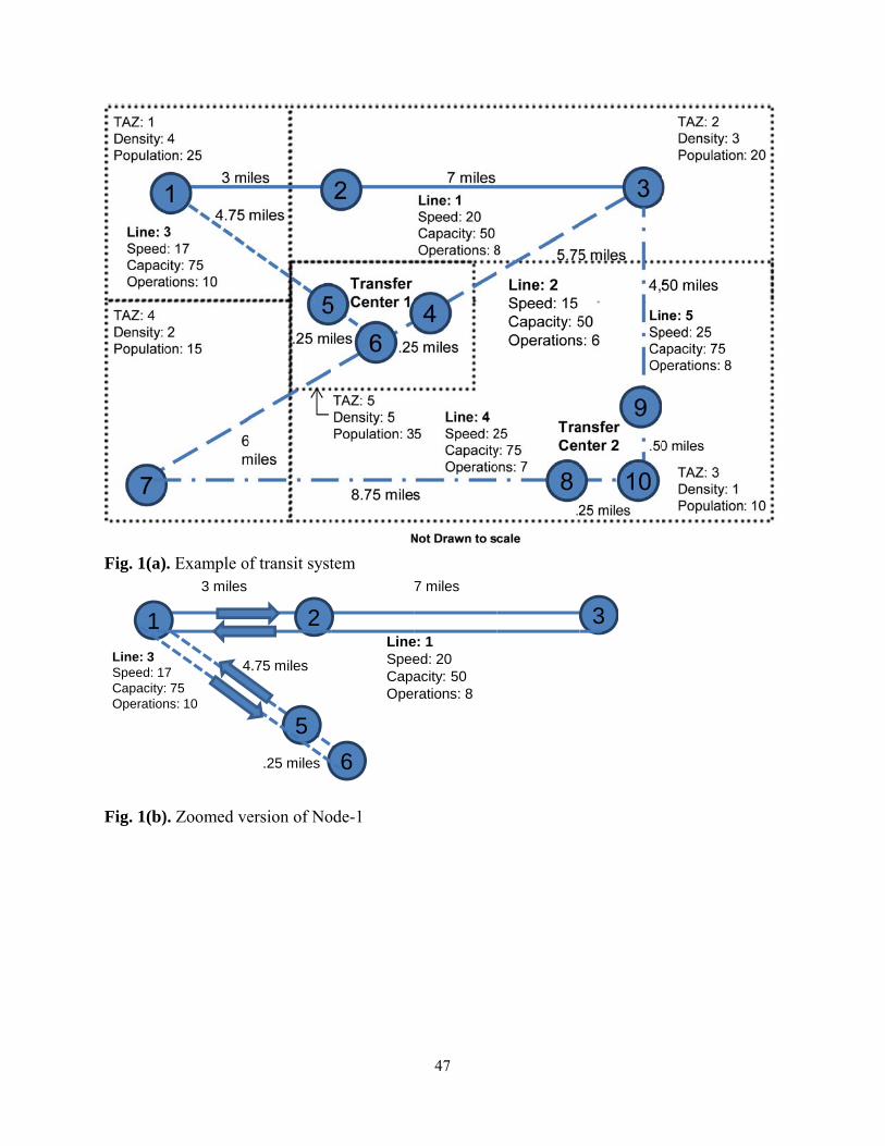
Fig. 1(a)

Fig. 1(b)

1Line: 3Speed: 17Capacity:Operation

. Example o

). Zoomed ve

3 miles

47: 75ns: 10

of transit syst

ersion of No

4.75 miles

2

5.25 miles

tem

ode-1

LineSpeeCapaOpe

6

47

7 miles

e: 1ed: 20acity: 50rations: 8

3

 

48  

Fig. 2(a). Thematic of the transit lines in Washington DC Fig. 2(b). Thematic of the transit lines in Baltimore  

 

 

 

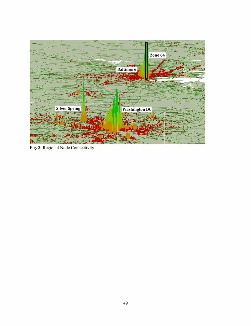
Fig. 3. Re

 

 

egional Node Connectivity

 

y

49

 

50  

Fig. 4. Node Connectivity

Node: 5841 

 

51  

Fig. 5. Washington transit line index

 

52  

Fig. 6. Baltimore transit line index

 

53  

Fig. 7. Regional rail index

 

54  

Fig. 8. Regional bus index

 

55  

Fig. 9. Regional connectivity index

   

 

56  

 

Appendix-I: Notations for Transit Connectivity

Notation Explanation : Degree of centrality of node n : Closeness Centrality : Eigenvector centrality of node n

: Inbound distance of link l : Outbound distance of link l from node n to destination

, : Shortest distance between node n1 to n

, Inbound connecting power of link l

. : Outbound connecting power of link l

, : Total connecting power of line l at node n : Set of stops in region R : Set of stops in line l : Set of stops in transfer center   : Set of stops in region center : Average Speed of link l : Initial stop

, : Transfer time from n1 to n

, : Total number of paths between n1 and n2

, : Number of paths exist between n1 and n2 those pass through n

: A binary indicator variable for determining the degree centrality, which takes the value of 1 when node p is dependent on n, and 0 otherwise

: Connectivity index for region R : Connectivity index for line l : Connectivity index for node n : Connectivity index for transfer center , : Passenger acceptance rate from node n1 to n : Density measure for region R

a : Parameter for passenger acceptance rate b : Parameter for passenger acceptance which is sensitive to travel time L : link N : Node N : Network system P : Node dependent on n

: Scaling factor coefficient for Capacity of line l : Scaling factor coefficient for Speed of line l : Scaling factor coefficient for distance of line l : Eigenvalue

, : Activity density of line l, at node n : Scaling factor for activity density

, : Number of households in zone z containing line l and node n

, : Employment for zone z containing line l and node n Θ , : Area of z containing line l and node Θ   : Number of lines l at node n