Embed Size (px)
Citation preview

ISSN 0956-8549-604
Performance Measurement and Evaluation
By
Bruce Lehmann Allan Timmermann
DISCUSSION PAPER NO 604
DISCUSSION PAPER SERIES
April 2007 Professor Lehmann is a Professor of Economics and Finance at the Graduate School of International Relations and Pacific Studies and is currently a Visiting Professor in the Division of Humanities and Social Sciences at the California Institute of Technology. Lehmann is a specialist in financial economics, with expertise in the pricing of capital assets, their volatility, and the markets in which they trade. He is the managing editor of the Journal of Financial Markets and the director of the Market Microstructure Research Group at the National Bureau of Economic Research. Allan Timmermann holds the Atkinson/Epstein Chair at the Rady School of Management and is also a professor of Economics at UCSD. His work focuses on asset pricing, portfolio allocation, performance measurement for mutual funds and pension funds and on topics in forecasting and time-series econometrics. Any opinions expressed here are those of the authors and not necessarily those of the FMG. The research findings reported in this paper are the result of the independent research of the authors and do not necessarily reflect the views of the LSE.

Performance Measurement and Evaluation
Bruce Lehmann
UCSD
Allan Timmermann
UCSD
April 7, 2007
Abstract
We consider performance measurement and evaluation for managed funds. Similarities
and differences−both in econometric practice and in interpretation of outcomes of empiricaltests−between performance measurement and conventional asset pricing models are analyzed.We also discuss how inference on ‘skill’ is affected when fund managers have market timing
information. Performance testing based on portfolio weights is also covered as is recent devel-
opments in Bayesian models of performance measurement that can accommodate errors in the
benchmark asset pricing model.
1 Introduction
Mutual funds are managed portfolios that putatively offer investors a number of benefits. Some
of them fall under the rubric of economies of scale such as the amortization of transactions and
other costs across numerous investors. The most controversial potential benefit, however, remains
the possibility that some funds can “beat the market.” The lure of active management is the
modern equivalent of alchemy, with the transformation of lead into gold replaced by hope that
the combination of specialized insights and superior information can result in portfolios that can
outperform the market. Hence, mutual fund performance evaluation − and, more generally, the
evaluation of the performance of managed portfolios − is all about measuring performance to
differentiate those managers who truly add value through active management from those who do
not.
How would a financial economist naturally address this question? The answer lies in a basic
fact that can be easily overlooked amid the hyperbole associated with the alleged benefits of active
1

management: mutual funds simply represent a potential increase in the menu of assets available
to investors. Viewed from this perspective, it is clear which tools of modern finance should be
brought to bear on performance evaluation: (1) the theory of portfolio choice and, to a lesser
extent, the equilibrium asset pricing theory that follows, in part, from it and (2) the no-arbitrage
approach to valuation.
Indeed, there are many similarities between the econometrics of performance measurement and
that of conventional asset pricing. Jensen’s alpha in performance measurement is just mispricing
in asset pricing models, we test for their joint significance using mean-variance efficiency or Euler
equation tests, using benchmark portfolios that are the (conditionally) mean-variance efficient
portfolios implied by such models or, almost equivalently, via their associated stochastic discount
factors. Similarly, the distinction between predictability in performance and its converse of no
persistence must often be handled with care in both settings.
The mechanical difference between the two settings lies in the asset universe: managed portfo-
lios with given weights in the performance literature as opposed to individual securities or portfolios
chosen by financial econometricians, not by portfolio managers, in the asset pricing literature. This
mechanical difference is of paramount economic importance: it is the fact that regularities observed
in the moments of the returns of managed portfolios are the direct consequence of explicit choices
made by the portfolio manager that makes the setting so different. To be sure, corporate officers,
research analysts, investors, traders, and speculators all make choices that affect the stochastic
properties of individual asset and aggregate passive portfolio returns. However, they do not do
so in the frequent, routine, and direct way that is the norm in the high turnover world of active
portfolio management. These pages have been literally littered with examples of ways in which
the direct impact of investment choices makes concerns like stochastic betas and the measurement
of biases in alphas first order concerns.
Managed portfolios are therefore not generic assets, which makes performance evaluation dis-
tinct from generic applications of modern portfolio theory in some dimensions. Chief among these
is the question of whether active managers add value, making one natural null hypothesis that
active managers do not add value or, in other words, that their funds do not represent an increase
in the menu of assets available to investors. Another difference is in the kind of abilities we
imagine that those active managers who do add value possess: market timing ability as opposed
to skill in security selection. In contrast, rejections of the null in asset pricing theory tests are
2

typically attributed to failures of the model. Others include the economic environment − that is,
the industrial organization of the portfolio management industry − confronting managers, the need
for performance measures that are objective and, thus, not investor specific, and differences in the
stochastic properties of managed portfolio returns as compared with individual assets and generic
passive portfolios.
The fact that managed portfolios’ performance is the outcome of the explicit choices of fund
managers also opens up the possibility of studying these choice variables explicitly when data is
available on portfolio composition. Tests for the optimality of a fund manager’s choice of portfolio
weights are available in these circumstances, although it is difficult to use this type of data in a
meaningful way unless the manager’s objective function is known. This is a problem, for example,
when assessing the asset/liability management skill of pension funds when data is available on asset
holdings but not on liabilities.
Our paper focuses on the methodological themes in the literature on performance measurement
and evaluation and only references the empirical literature sparingly, chiefly to support arguments
about problems with existing methods. We present a unified framework for understanding existing
methods and offer some new results as well. We do not aim to provide a comprehensive survey
of the empirical literature, which would call for a different paper altogether. We refer readers to
Cuthbertson et al (2007) for a recent survey of the empirical evidence of mutual funds.
The outline of the remainder of the paper is as follows. Section 2 establishes theoretical bench-
marks for performance benchmarks in the context of investors’ marginal investment decisions,
discusses sources of benchmarks, and introduces some performance measures in common use. Sec-
tion 3 provides an analysis of performance measurement in the presence of market timing and
time-variations in the fund manager’s risk exposures. As part of our analysis, we cover a range
of market timing specifications that involve different sorts of market timing information signals.
Section 4 looks at performance measures in the presence of data on portfolio weights. Section 5
falls under the broad title of the cross-section of managed portfolio returns. It covers standard
econometric approaches and test statistics for detecting abnormal performance both at the level of
individual funds and also for the cross-section of funds or sub-groups of (ranked) funds. Finally,
Section 6 discusses recent Bayesian contributions to the literature and Section 7 concludes.
3

2 Theoretical Benchmarks
Our analysis of the measurement of the performance of managed portfolios begins with generic
investors with common information and beliefs who equate the expected marginal cost of investing
(in utility terms) with expected marginal benefits. Without being specific about where it comes
from, assume that an arbitrary investor’s indirect utility of wealth, Wt, is given by V (Wt,xt),
where xt is a generic state vector that might include other variables (including choice variables)
that impinge on the investor’s asset allocation decision, permitting utility to be state dependent
and nonseparable. Let pit and dit be the price and dividend on the ith asset (or mutual fund),
respectively, making the corresponding gross rate of returnRit+1 = (pit+1+dit+1)/pit. The marginal
conditions for this investor are given by
E
∙V 0(Wt+1,xt+1)
V 0(Wt,xt)Rit+1|It
¸≡ E[mt+1Rit+1|It] = 1, (1)
where It is information available to the investor at time t andmt+1 is the stochastic discount factor.
We assume that there is a riskless asset with return Rft+1 (known at time t) and so E[mt+1|It] =
R−1ft+1.
The investment decisions of any investor who maximizes expected utility can be character-
ized by a marginal decision of this form. The denominator is given by V0(Wt,xt)pit − the ex
post cost in utility terms of investing a little more in asset i − and the numerator is given by
V 0(Wt+1,xt+1)(pit+1 + dit+1), the ex post marginal benefit from making this incremental invest-
ment. Setting their expected ratio to one ensures that the marginal benefits and costs of investing
are equated. Note that nothing in this analysis relies on special assumptions about investor
preferences or about market completeness.
Now consider the conditional population projection of the intertemporal marginal rate of sub-
stitution of this investor mt+1 = V 0(Wt+1,xt+1)/V0(Wt,xt) on the N−vector of returns Rt+1 of
risky assets with returns that are not perfectly correlated:
mt+1 = δ0t + δ0tRt+1 + εmt+1
= R−1ft+1 + δ0t(Rt+1 −E[Rt+1|It]) + εmt+1 (2)
= R−1ft+1 +Cov(Rt+1,mt+1|It)0V ar(Rt+1|It)−1(Rt+1 −E[Rt+1|It]) + εmt+1
4

where, letting ι denote an N × 1 vector of ones,
δt = V ar(Rt+1|It)−1Cov(Rt+1,mt+1|It)
= V ar(Rt+1|It)−1(E[Rt+1mt+1|It]−E[Rt+1|It]E[mt+1|It]) (3)
= V ar(Rt+1|It)−1(ι−E[Rt+1|It]R−1ft+1).
It is convenient to transform δt into portfolio weights via ωδt = δt/δ0tι, which yields the associ-
ated portfolio returns Rδt+1 = ω0δtRt+1. In terms of the (conditional) mean/variance efficient set,
the weights of portfolio δ are given by
ωδt =V ar(Rt+1|It)−1(ι−E[Rt+1|It]R−1ft+1)ι0V ar(Rt+1|It)−1(ι−E[Rt+1|It]R−1ft+1)
=V ar(Rt+1|It)−1[ι−E(Rt+1|It)R−1ft+1]
(ct − bR−1ft+1)
=Rft+1
Rft+1 −E[R0t+1|It]ω0t −
E[R0t+1|It]Rft+1 −E[R0t+1|It]
ωst
= ω0t +E(R0t+1|It)
E(R0t+1|It)−Rft+1(ωst − ω0t), (4)
where ω0t = V ar(Rt+1|It)−1ι/ct is the vector of portfolio weights of the conditional minimum vari-
ance portfolio, R0t+1 is the corresponding minimum variance portfolio return, ct = ι0V ar(Rt+1|It)−1ι,
bt = ι0V ar(Rt+1|It)−1E(Rt+1|It)R−1ft+1 and ωst = V ar(Rt+1|It)−1E(Rt+1|It)/bt is the weight vec-
tor for the maximum squared Sharpe ratio portfolio.
None of the variables in this expression for the conditional regression coefficients δt are investor
specific. All investors who share common beliefs about the conditional mean vector and covariance
matrix of the N asset returns and who are on the margin with respect to these N assets will agree
on the values of the elements of δt irrespective of their preferences, other traded and nontraded
asset holdings, or any other aspect of their economic environment. Put differently, portfolio δ is
the optimal portfolio of these N assets for hedging fluctuations in the intertemporal marginal rates
of substitution of any marginal investor. Similarly, all investors who are marginal with respect to
these N assets will perceive that expected returns satisfy
E[Rt+1 − ιRft+1|It] = βδtE[Rδt+1 − ιRft+1|It], (5)
since δ is a conditionally mean-variance efficient portfolio.1
1What is lost in the passage from the intertemporal marginal rate of substitution to portfolio δ? The answer
5

There is another way to arrive at the same benchmark portfolios: the application of the no-
arbitrage approach to the valuation of risky assets. Once again, begin with N risky assets with
imperfectly correlated returns. Asset pricing based on the absence of arbitrage typically involves
three assumptions in addition to the definition of an arbitrage opportunity:2 (1) investors perceive
a deterministic mapping between end-of-period asset payoffs and underlying states of nature s; (2)
agreement on the possible; and (3) the perfect markets assumption. The first condition is met
almost by construction if investors identify states with the array of all possible payoff patterns. The
second asserts that no investor thinks any state is impossible since such an investor would be willing
to sell an infinite number of claims that pay off in that state. The perfect markets assumption
− that is, the absence of taxes, transactions costs, indivisibilities, short sales restrictions, or other
impediments to free trade − is problematic since it is obviously impossible to sell managed portfolios
short to create zero net investment portfolios.
Fortunately, there is an alternative to the absence of short sale constraints that eliminates this
concern. Any change in the weights of a portfolio that leaves its cost unchanged is a zero net
investment portfolio. Hence, arbitrage reasoning can be used when there are investors who are
long the assets under consideration. All that is required to implement the no-arbitrage approach
to valuation is the existence of investors with long positions in each asset who can costlessly make
marginal changes in existing positions. In unfettered markets, the substitution possibilities of a few
investors can replace the marginal decisions of many when the few actively seek arbitrage profits
in this asset menu.
It is now a simple matter to get from these assumptions to portfolio δ. The absence of arbitrage
coupled with some mild regularity conditions (such as investors prefer more to less) when there is
a continuum of possible states implies the existence of strictly positive state prices, not necessarily
unique, that price the N assets under consideration as in:
pit =
Zψt+1(s) [pit+1(s) + dit+1(s)] ds (6)
is simple: while the realizations of mt+1 are strictly positive since it is a ratio of marginal utilities, the returns
of portfolio δ need not be strictly positive since its weights need not be positive (i.e., portfolio δ might have short
positions). As a practical matter, the benchmark portfolios used in practice seldom have short positions.2We have ignored the technical requirement that there be at least one asset with positive value in each state
because managed portfolios and, for that matter, most traded securities are limited liability assets.
6

where s indexes states and ψt+1(s) is the (not necessarily unique) price at time t of a claim that
pays one dollar if state s occurs at time t + 1 and zero otherwise. Letting πt+1(s) denote the
(conditional) probability at time t that state s will occur at time t + 1, this expression may be
rewritten as:
pit =
Zπ(s)
ψt+1(s)
πt+1(s)[pit+1(s) + dit+1(s)] ds
≡Z
πt+1(s)mt+1(s) [pit+1(s) + dit+1(s)] ds
≡ E[mt+1(pit+1 + dit+1)|It], (7)
where mt+1(s) = ψ(s)/π(s) is a strictly positive random variable − that is, both state prices and
probabilities are strictly positive − with realizations given by state prices per unit probability,
which is termed a stochastic discount factor in the literature. All that remains is to project any
stochastic discount factormt+1 that reflect common beliefs πt+1(s) − where the word “any” reflects
the fact that state prices need not be unique − onto the returns of the N assets to recover portfolio
δ.
As was noted above, there is at least one reason for taking this route: to make it clear that the
existence of portfolio δ does not require all investors to be on the margin with respect to these N
assets. Many, even most, investors may be inframarginal but some investors must be (implicitly)
making marginal decisions in these assets for this reasoning to apply. Chen and Knez (1996) reach
the same conclusion in their analysis of arbitrage-free performance measures.3
These considerations make portfolio δ a natural candidate for being the benchmark portfolio
against which investment performance should be measured for investors who are skeptical regarding
the prospects for active management. It is appropriate for skeptics precisely because managed
portfolios are given zero weight in portfolio δ. Put differently, this portfolio can be used to answer
3More precisely, they search for performance measures that satisfy four desiderata: (1) the performance of any
portfolio that can be replicated by a passively managed portfolio with weights based only on public information
should be zero, (2) the measure should be linear (i.e., the performance of a linear combination of portfolios should be
the linear combination of the individual portfolio measures), (3) it should be continuous (i.e., portfolios with similar
returns state by state should have similar performance measures), and (4) it should be nontrivial and assign a non-
zero value − that is, a positive price − to any traded security. They show that these four conditions are equivalent
to the absence of arbitrage and the concomitant existence of state prices or, equivalently, strictly stochastic discount
factors.
7

the question of whether such investors should take small positions in a given managed portfolio.4 As
noted above, it is an objective measure in that investors with common beliefs about the conditional
mean vector and covariance matrix will agree on the composition of δ. Thus, we have identified a
reasonable candidate benchmark portfolio for performance measurement.
What benchmark portfolio is appropriate for investors who are not skeptical about the existence
of superior managers? One answer lies in an observation made earlier: such investors would
naturally think that managed portfolios represent a nontrivial enlargement of the asset menu.
That is, portfolio δ would change in its composition as it would place nonzero weight on managed
portfolios if they truly added value by improving investors’ ability to hedge against fluctuations in
their intertemporal marginal rate of substitution. Like the managed-portfolio-free version of δ, it
is an objective measure for investors who share common beliefs about conditional means, variances,
and covariances of returns in this enlarged asset menu.
2.1 Sources of Benchmarks
There is an apparent logical conundrum here: it would seem obvious that managed portfolios
either do or do not improve the investment opportunities available to investors. The answer, of
course, is that it is difficult to estimate the weights of portfolio δ with any precision in practice.
The required inputs are the conditional mean vector E[Rt+1|It] and the conditional covariance
matrix V ar(Rt+1|It) of these N assets. Unconditional mean stock returns cannot be estimated
with precision due to the volatility of long-lived asset returns and the estimation of conditional
means adds further complications. Unconditional return variances and covariances are measured
with greater precision but the curse of dimensionality associated with the estimation of the inverse
of the conditional covariance matrix limits asset menus to ten or twenty assets at most − a number
far fewer than the number of securities in typical managed portfolios.
This is one reason why benchmark portfolios are frequently specified in advance according
to an asset pricing theory. In particular, most asset pricing theories imply that intertemporal
marginal rates of substitution are linear combinations of particular portfolios. The Sharpe-Lintner-
Mossin CAPM implies that mt+1 is linear in the return of the market portfolio of all risky assets.
4This point is not quite right as stated because investors can only make marginal changes in one direction when
they cannot sell managed portfolios short. The statement is correct once one factors in the existence of an investor
who is long the fund in question and can make marginal changes in both directions.
8

In the consumption CAPM, the single index is the portfolio with returns that are maximally
correlated with aggregate consumption growth, sometimes raised to some power. Other asset
pricing models imply that mt+1 is linear in the returns of other portfolios. In the CAPM with
nontraded assets, the market portfolio is augmented with the portfolio of traded assets with returns
that are maximally correlated with nontraded asset returns. The indices in the intertemporal
CAPM are the market portfolio plus portfolios with returns that are maximally correlated with the
state variables presumed to drive changes in the investment opportunity set. The APT also specifies
that mt+1 is (approximately) linear in the returns of several portfolios, well-diversified portfolios
that are presumed to account for the bulk of the (perhaps conditional) covariation among asset
returns.
In practice, chosen benchmarks typically reflect the empirical state of asset pricing theory and
constraints on available data. For example, we do not observe the returns of “all risky assets” −
that is, aggregate wealth − but stock market wealth in the form of the S&P 500 and the CRSP
value-weighted index is observable and, at one time, appeared to price most assets pretty well.
Before that, the single index market model was used to justify using the CRSP equally-weighted
index as a market proxy while the APTmotivates the use of multiple well-diversified portfolios. The
empirical success of models like the three-factor Fama-French model − a market proxy along with
size and market-to-book portfolios as benchmarks − and, more recently, the putatively anomalous
returns to momentum portfolios, have been added to the mix as a fourth factor.
Irrespective of the formal justification, such benchmarks take the form of a weighted average of
returns on a set of factors, fkt+1:
mt+1 =KXk=1
ωktfkt+1, (8)
where this relation differs from the projection (2) in having no error term. That is, the stochastic
discount factor is assumed to be an exact linear combination of observables. In the case of the
multifactor benchmarks, the weights are usually treated as unknowns to be estimated, as is the case
with portfolio δ save for the fact that there are only K weights to be estimated in this case. This
circumstance arises because most multifactor models, both the APT and the ad hoc models like
the Fama-French model, do not specify the values of risk premiums, which are intimately related
to the weights ωkt. In contrast, equilibrium models do typically specify the relevant risk premiums
and, implicitly, the weights ωkt. For example, letting Rmt+1 be the return on the market portfolio,
9
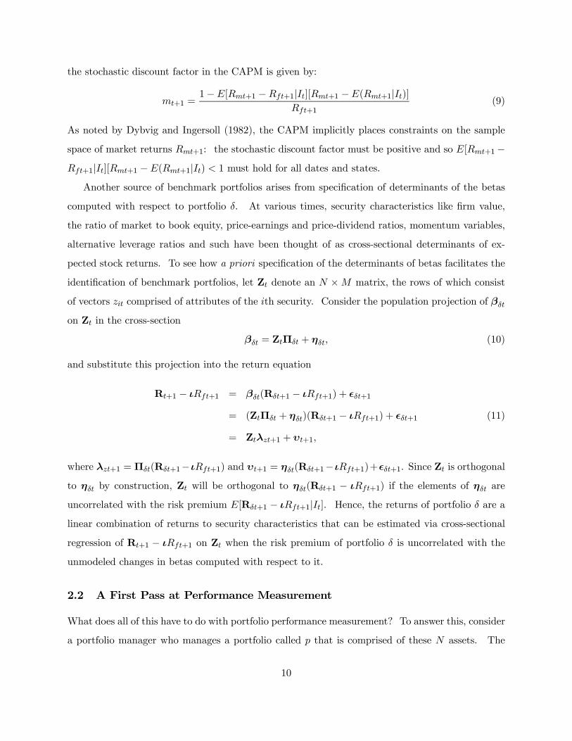
the stochastic discount factor in the CAPM is given by:
mt+1 =1−E[Rmt+1 −Rft+1|It][Rmt+1 −E(Rmt+1|It)]
Rft+1(9)
As noted by Dybvig and Ingersoll (1982), the CAPM implicitly places constraints on the sample
space of market returns Rmt+1: the stochastic discount factor must be positive and so E[Rmt+1−
Rft+1|It][Rmt+1 −E(Rmt+1|It) < 1 must hold for all dates and states.
Another source of benchmark portfolios arises from specification of determinants of the betas
computed with respect to portfolio δ. At various times, security characteristics like firm value,
the ratio of market to book equity, price-earnings and price-dividend ratios, momentum variables,
alternative leverage ratios and such have been thought of as cross-sectional determinants of ex-
pected stock returns. To see how a priori specification of the determinants of betas facilitates the
identification of benchmark portfolios, let Zt denote an N ×M matrix, the rows of which consist
of vectors zit comprised of attributes of the ith security. Consider the population projection of βδt
on Zt in the cross-section
βδt = ZtΠδt + ηδt, (10)
and substitute this projection into the return equation
Rt+1 − ιRft+1 = βδt(Rδt+1 − ιRft+1) + ²δt+1
= (ZtΠδt + ηδt)(Rδt+1 − ιRft+1) + ²δt+1 (11)
= Ztλzt+1 + υt+1,
where λzt+1 = Πδt(Rδt+1−ιRft+1) and υt+1 = ηδt(Rδt+1−ιRft+1)+²δt+1. Since Zt is orthogonal
to ηδt by construction, Zt will be orthogonal to ηδt(Rδt+1 − ιRft+1) if the elements of ηδt are
uncorrelated with the risk premium E[Rδt+1 − ιRft+1|It]. Hence, the returns of portfolio δ are a
linear combination of returns to security characteristics that can be estimated via cross-sectional
regression of Rt+1 − ιRft+1 on Zt when the risk premium of portfolio δ is uncorrelated with the
unmodeled changes in betas computed with respect to it.
2.2 A First Pass at Performance Measurement
What does all of this have to do with portfolio performance measurement? To answer this, consider
a portfolio manager who manages a portfolio called p that is comprised of these N assets. The
10

manager uses information Ipt to choose the weights ωpt. Suppose that the information available
to the manager is contained in the investor’s information set It (i.e., Ipt ⊆ It). Would an investor
whose portfolio holdings have been chosen to satisfy the marginal conditions E[mt+1Rit+1|It] = 1
find it desirable to divert some of the investment in the original N assets to this managed portfolio?
The answer is clearly no: the investor could have chosen ωpt as part of the original portfolio since
ωpt ∈ Ipt ⊆ It, since
E[mt+1Rpt+1|It] = E[mt+1ω0ptRt+1|It] = ω0ptE[mt+1Rt+1|It] = 1. (12)
Now consider the case in which the manager has access to information not available to the investor
so that wpt /∈ Ipt ⊆ It. In this case, the Euler equation need not hold − that is, E[mt+1Rpt+1|It]
need not equal one − if the information is available to investors only through the managed portfolio
p.
In particular, consider the (conditional) population projection of Rpt+1−Rft+1 on Rδt+1−Rft+1
and a constant:
Rpt+1 −Rft+1 = αpt + βpt(Rδt+1 −Rft+1) + εpt+1, (13)
where αpt and βpt are conditioned on It, the information available to the investor and not the
potentially richer information in the hands of the portfolio manager. Now consider the Euler
equation for p evaluated at the intertemporal marginal rate of substitution (or, equivalently, the
stochastic discount factor) after p has been added to the asset menu:
0 = E[mt+1(Rpt+1 −Rft+1)|It] = E[mt+1(αpt + βpt(Rδt+1 −Rft+1) + εpt+1)|It]
= R−1ft+1αpt +E[mt+1εpt+1|It] (14)
which implies that
αpt = −Rft+1E[mt+1εpt+1|It] (15)
Large values of αpt imply correspondingly large values of E[mt+1εpt+1|It], suggesting correspond-
ingly large gains from adding p to the asset menu in terms of hedging fluctuations in marginal
utilities. Put differently, δpt, the coefficient on Rpt+1 from the (conditional) population regression
of mt+1 on Rt+1 and Rpt+1, is given by:
δpt =E[εmt+1εpt+1|It]V ar(εpt+1|It)
=E[mt+1εpt+1|It]V ar(εpt+1|It)
= − αptRft+1V ar(εpt+1|It)
(16)
11

from the usual omitted variables formula. Large values of δpt also imply better marginal utility
hedging and δpt will be nonzero if and only if αpt is nonzero.
The regression intercept αpt is called the conditional Jensen measure in the performance evalu-
ation literature, the unconditional version of which was introduced in Jensen (1968, 1969).5 It has
a simple interpretation as the return on a particular zero net investment portfolio: that obtained
by purchasing one dollar of portfolio p and financing this acquisition by borrowing 1− βpt dollars
at the riskless rate and by selling βpt dollars of portfolio δ short. The Sharpe ratio of this portfolio
isαptp
V ar(εpt+1|It)which is proportional to the t−statistic for the difference of αpt from zero (the Sharpe ratio of any
zero net investment portfolio is its expected payoff scaled by the standard deviation of its payoff).
This Sharpe ratio is called the Treynor-Black (1973) appraisal ratio.
This role for the regression intercept also suggests that performance evaluation via Jensen
measures is fraught with hazard. A nonzero value of αpt could also reflect benchmark error. That
is, αpt would typically be nonzero if portfolio δ is not (conditionally) mean-variance efficient even
if the portfolio manager has no superior information and skill. Hence, it is often difficult to tell if
one is learning about the quality of the manager or the quality of the benchmark when examining
Jensen regressions. This is why the strictly correct interpretation of nonzero intercepts is that the
mean-variance trade-off based on portfolio δ and the riskless asset can be improved by augmenting
the asset menu to include portfolio p as well, not that the managed portfolio outperforms the
benchmark.
As noted earlier, portfolio δ might include or exclude portfolio p. The exclusion of portfolio
p from the asset menu corresponds to a thought experiment in which hypothetical investors with
no investment in this portfolio are using portfolio δ to evaluate the consequences of adding a small
amount of portfolio p to the asset menu. Similarly, the inclusion of portfolio p in the asset menu
used to construct portfolio δ corresponds to a thought experiment in which hypothetical investors
who have a position in portfolio p are assessing whether they have invested the correct amount in
5 Interestingly, Jensen did not motivate the use of the CRSP equally-weighted portfolio solely by reference to the
CAPM. He coupled this justification with the observation that its returns would well approximate the returns on
aggregate wealth if returns follow a single factor model, implicitly making his reasoning a progenitor of one factor
versions of the equilibrium APT.
12

it. In the language of hypothesis testing, the former approach corresponds to a Lagrange multiplier
test of the null hypothesis of no abnormal performance while the latter corresponds to a Wald test
when testing the hypothesis that the weight on p should be zero. The pervasive adoption of the
former approach in the performance evaluation literature probably reflects general skepticism in
the profession on the economic value of active management. It is as though we believe that asset
prices are set in an efficient market but that the market for active managers who earn abnormal
fees is inefficient.
Finally, the Sharpe ratio to which we referred above represents a non-benchmark-based approach
to performance measurement. In its conditional form, the Sharpe ratio of portfolio p is given by:
E[Rpt+1 −Rft+1|It]pV ar[Rpt+1|It]
which is the conditional mean return divided by its standard deviation of a dollar invested in
portfolio p that is financed by borrowing a dollar at the riskless rate. The Sharpe ratio got its
start in Sharpe (1966) as a simple and intuitive measure of how far a given portfolio was from the
mean/variance efficient frontier.
Over time, it has become clear that the measurement of the distance between a given portfolio
and the mean/variance efficient frontier is quite a bit more subtle, involving Jensen’s alpha in an
unexpected way (see, for example, Jobson and Korkie (1982) and Gibbons, Ross, and Shanken
(1989)). We noted earlier that αpt is the expected return of a portfolio that is long one dollar of
portfolio p and short βpt dollars of portfolio δ and 1− βpt dollars of the riskless asset, which makes
it a costless and zero beta portfolio. As such, it is a means to get to the mean/variance efficient
frontier through a suitable combination of the N given assets, the riskless asset, and this costless
zero beta portfolio. This reasoning extends toM additional managed portfolios in a straightforward
way.
This has left the Sharpe ratio in a sort of intellectual limbo. The simple intuition has survived
and the practitioner literature and, perhaps more importantly, performance measurement in prac-
tice often refers to the Sharpe ratio. It has fallen out of fashion in the academic literature since we
now understand its deficiencies much better. It is simply not the case that managed portfolio A is
better than B if its Sharpe ratio is higher because the distance to the frontier depends on portfolio
alphas and residual variances and covariances, not on the mean and variance of overall portfolio
13

returns. Benchmark-based performance measurement is the focus of the academic literature and
practitioners who use Sharpe ratios generally do so in conjunction with Jensen alphas, often under
the rubric of tracking error.
3 Performance Measurement and Market Timing
The conditional Jensen regression (13) differs from the original in Jensen (1968, 1969) in only two
details: the Jensen alpha αpt and portfolio beta βpt are conditional and not unconditional moments
and the benchmark portfolio is δ and not ”the market portfolio of all risky assets” underlying the
CAPM. There is an important commonality with the original since it is natural to decompose
returns into two components, that related to benchmark or market returns − that is, βpt(Rδt+1 −
Rft+1) − and that unrelated to them − that is, αpt+εpt+1. By analogy with the older parlance, we
can term the first component the return to market timing and, under this interpretation, the second
component must reflect the rewards to security selection. The distinction between market timing
and security selection permeates both the academic and practitioner literatures on performance
attribution and evaluation.
The impact of real or imagined market timing ability on performance measurement depends
on whether the return generating process experiences time variation. That is, the benchmark
beta βpt might change because of time-variation in individual security betas and not because the
manager is attempting to time the market. Similarly, the expected returns of portfolio p might
also change if E[Rδt+1−Rft+1|It] varied over time. Moreover, the manager might choose to make
portfolio betas shift along with changes in benchmark portfolio volatility or other higher moments.
Accordingly, we must distinguish between the case in which excess benchmark returns are serially
independent from the perspective of uninformed portfolio managers from those in which there is
serial dependence (predictability) based on public information.
Accordingly, consider first the case in which the manager of portfolio p does not attempt
to time the market and the conditional benchmark risk premium is time invariant − that is,
E[Rδt+1−Rft+1|It] = E[Rδt+1−Rft+1]. Since the fund has a constant target beta βp, the original
unconditional Jensen regression:
Rpt+1 −Rft+1 = αp + βp(Rδt+1 −Rft+1) + pt+1 (17)
is related to that from the conditional Jensen regression (13) via:
14

pt+1 = αpt − αp + εpt+1 (18)
where αp ≡ E[αpt] is the unconditional Jensen performance measure. This is a perfectly well-posed
regression with potentially serially correlated and heteroskedastic disturbances, although there are
economic settings in which market efficiency requires αpt − αp to be unpredictable. Hence, one
can estimate αp and βp consistently in these circumstances and so the Jensen measure correctly
measures the rewards to security selection.
Unsuccessful market timing efforts complicate performance attribution, but not performance
measurement per se, when expected excess benchmark returns are constant. If the manager shifts
betas but has no market timing ability, the composite error pt+1 in the population is now given
by:
pt+1 = αpt − αp + (βpt − βp)(Rδt+1 −Rft+1) + εpt+1 (19)
which has unconditional mean zero because:
E[ pt+1] = E[αpt − αp + (βpt − βp)(Rδt+1 −Rft+1) + εpt+1]
= E[(βpt − βp)(Rδt+1 −Rft+1)] (20)
= Cov[βpt, Rδt+1 −Rft+1]
is equal to zero unless the manager has market timing ability. Once again, the unconditional
Jensen regression will yield consistent estimates of the unconditional beta βp and Jensen measure
αp.6 The residual, however, is no longer solely a reflection of the security selection component of
returns.
Problems crop up when managers engage in efforts to time the market and they are successful
(on average) in doing so. Once again, the unconditional Jensen measure is given by (17):
αp = E[Rpt+1 −Rft+1 − βp(Rδt+1 −Rft+1)]
= E[αpt + (βpt − βp)(Rδt+1 −Rft+1) + εpt+1]
= E[αpt] + Cov[βpt, Rδt+1 −Rft+1]
6The fact that the residual is conditionally heteroskedastic and, perhaps, serially correlated due to the αpt − αp
and (βpt − βp)(Rδt+1 −Rft+1) terms suggests that some structure might be placed on their stochastic properties to
draw inferences about their behavior. An example of this sort is presented in the next section.
15

so that the sign and magnitude of the unconditional alpha depends on the way in which the manager
exploits market timing ability. The coefficient αp will measure the reward to security selection
only if the manager uses this skill to give the portfolio a constant beta, in which case pt+1 correctly
measures the return to security selection.
Otherwise, the Jensen measure will reflect both market timing and security selection ability
when managers are successful market timers, thus breaking the clean decomposition of returns into
security selection and market timing. The Jensen alpha will be positive if the manager uses market
timing to improve portfolio performance − that is, to have a higher expected return than that
which can be gained solely from security selection ability − by setting Cov[βpt, Rδt+1−Rft+1] > 0
but the Jensen measure alone cannot be used to decompose performance into market timing and
security selection components. Similarly, market timing efforts can yield a negative Jensen alpha
when the manager tries to make the fund countercyclical by setting Cov[βpt, Rδt+1 − Rft+1] < 0.
This last possibility is not a pathological special case: managers with market timing ability who
minimize portfolio variance for a given level of unconditional expected excess returns will tend to
have portfolio betas that are negatively correlated with benchmark risk premiums. The observation
that a negative estimate of Jensen’s alpha can result from market timing skills has been made by,
inter alia, Jensen (1972), Admati and Ross (1985) and Dybvig and Ross (1985).
Performance measurement and attribution is even more complicated when there is serial depen-
dence in returns from the perspective of managers without market timing ability. The reason is
obvious: such managers can make their betas dependent on conditional expected excess benchmark
returns. That is, managed portfolios can have time-varying expected returns and betas conditional
on public information, not just private information. In particular, Cov[βpt, Rδt+1 − Rft+1] need
not be zero even in the absence of market timing ability since:
Cov[βpt, Rδt+1 −Rft+1] = E[(βpt − βp)[(Rδt+1 −Rft+1)−E(Rδt+1 −Rft+1|It)]]
+E[(βpt − βp)[E(Rδt+1 −Rft+1|It)−E(Rδt+1 −Rft+1)]]
= Cov[βpt, Rδt+1 −Rft+1|It] + Cov[βpt, E(Rδt+1 −Rft+1|It)] (21)
can be nonzero both in the presence of market timing ability, which makes the first term nonzero,
and of portfolio betas that are correlated with shifts in the benchmark risk premium, which makes
the second term nonzero. Once again, there is no simple decomposition of portfolio returns into
security selection and market timing components based on managed portfolio returns alone when
16
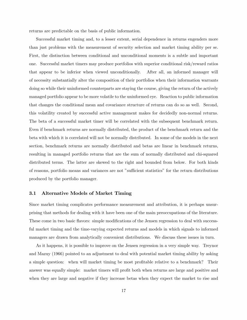
returns are predictable on the basis of public information.
Successful market timing and, to a lesser extent, serial dependence in returns engenders more
than just problems with the measurement of security selection and market timing ability per se.
First, the distinction between conditional and unconditional moments is a subtle and important
one. Successful market timers may produce portfolios with superior conditional risk/reward ratios
that appear to be inferior when viewed unconditionally. After all, an informed manager will
of necessity substantially alter the composition of their portfolios when their information warrants
doing so while their uninformed counterparts are staying the course, giving the return of the actively
managed portfolio appear to be more volatile to the uninformed eye. Reaction to public information
that changes the conditional mean and covariance structure of returns can do so as well. Second,
this volatility created by successful active management makes for decidedly non-normal returns.
The beta of a successful market timer will be correlated with the subsequent benchmark return.
Even if benchmark returns are normally distributed, the product of the benchmark return and the
beta with which it is correlated will not be normally distributed. In some of the models in the next
section, benchmark returns are normally distributed and betas are linear in benchmark returns,
resulting in managed portfolio returns that are the sum of normally distributed and chi-squared
distributed terms. The latter are skewed to the right and bounded from below. For both kinds
of reasons, portfolio means and variances are not ”sufficient statistics” for the return distributions
produced by the portfolio manager.
3.1 Alternative Models of Market Timing
Since market timing complicates performance measurement and attribution, it is perhaps unsur-
prising that methods for dealing with it have been one of the main preoccupations of the literature.
These come in two basic flavors: simple modifications of the Jensen regression to deal with success-
ful market timing and the time-varying expected returns and models in which signals to informed
managers are drawn from analytically convenient distributions. We discuss these issues in turn.
As it happens, it is possible to improve on the Jensen regression in a very simple way. Treynor
and Mazuy (1966) pointed to an adjustment to deal with potential market timing ability by asking
a simple question: when will market timing be most profitable relative to a benchmark? Their
answer was equally simple: market timers will profit both when returns are large and positive and
when they are large and negative if they increase betas when they expect the market to rise and
17

shrink or choose negative betas when they expect the market to fall. Since squared returns will be
large in both circumstances, modifying the Jensen regression to include squared benchmark returns
can facilitate the measurement of both market timing and security selection ability.
Accordingly, consider the Treynor-Mazuy quadratic regression:
Rpt+1 −Rft+1 = ap + b0p(Rδt+1 −Rft+1) + b1p(Rδt+1 −Rft+1)2 + ζpt+1
and suppose that the manager has a constant unconditional beta βp, so that βpt = βp + ξβpt is
a choice variable for the manager and not the conditional beta based on public information as in
(13).7 Substitution of this variant of the conditional Jensen regression into the normal equations
for the quadratic regression reveals that the unconditional projection coefficients b0p and b1p are
given by:⎛⎝ b0p
b1p
⎞⎠ =
⎡⎣V ar⎛⎝ Rδt+1 −Rft+1
(Rδt+1 −Rft+1)2
⎞⎠⎤⎦−1Cov⎡⎣Rpt+1 −Rft+1,
⎛⎝ Rδt+1 −Rft+1
(Rδt+1 −Rft+1)2
⎞⎠⎤⎦=
⎛⎝ βp
0
⎞⎠+ 1
σ2δσ4δ − σ23δ
⎛⎝ σ4δ −σ3δ−σ3δ σ2δ
⎞⎠×
⎛⎝ Cov[ξβpt , (Rδt+1 −Rft+1)2] + Cov[αpt, Rδt+1 −Rft+1]
Cov[ξβpt , (Rδt+1 −Rft+1)3] + Cov[αpt, (Rδt+1 −Rft+1)
2]
⎞⎠≡
⎛⎝ βp
0
⎞⎠+⎛⎝ γ0p
γ1p
⎞⎠ , (22)
where σ3δ and σ4δ are the unconditional skewness and kurtosis of excess benchmark returns, re-
spectively. Similarly, the quadratic regression intercept ap is given by:
ap = αp + Cov[ξβpt , Rδt+1 −Rft+1]− γ0pE[Rδt+1 −Rft+1]− γ1pE[(Rδt+1 −Rft+1)2]. (23)
As was the case earlier, it is convenient to separate the analysis into two cases: that in which
excess benchmark returns are serially independent and that in which they are serially dependent.
We discuss these cases in turn.
Before doing so, however, we must address the role of αpt in understanding market timing skills.
To the best of our knowledge, no paper in the performance evaluation literature has contemplated
the possibility that the conditional Jensen measure αpt is correlated with the conditional moments
7The target beta could be time-varying as long as its value is known by uninformed investors.
18
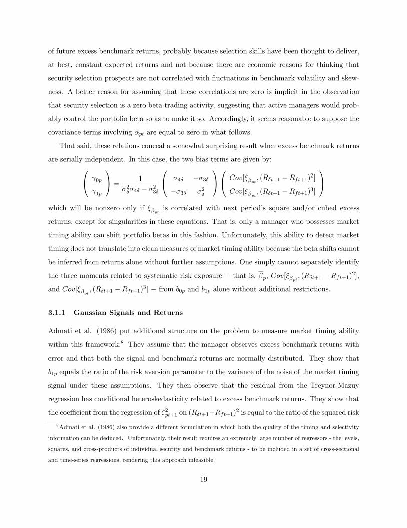
of future excess benchmark returns, probably because selection skills have been thought to deliver,
at best, constant expected returns and not because there are economic reasons for thinking that
security selection prospects are not correlated with fluctuations in benchmark volatility and skew-
ness. A better reason for assuming that these correlations are zero is implicit in the observation
that security selection is a zero beta trading activity, suggesting that active managers would prob-
ably control the portfolio beta so as to make it so. Accordingly, it seems reasonable to suppose the
covariance terms involving αpt are equal to zero in what follows.
That said, these relations conceal a somewhat surprising result when excess benchmark returns
are serially independent. In this case, the two bias terms are given by:⎛⎝ γ0p
γ1p
⎞⎠ =1
σ2δσ4δ − σ23δ
⎛⎝ σ4δ −σ3δ−σ3δ σ2δ
⎞⎠⎛⎝ Cov[ξβpt , (Rδt+1 −Rft+1)2]
Cov[ξβpt , (Rδt+1 −Rft+1)3]
⎞⎠which will be nonzero only if ξβpt is correlated with next period’s square and/or cubed excess
returns, except for singularities in these equations. That is, only a manager who possesses market
timing ability can shift portfolio betas in this fashion. Unfortunately, this ability to detect market
timing does not translate into clean measures of market timing ability because the beta shifts cannot
be inferred from returns alone without further assumptions. One simply cannot separately identify
the three moments related to systematic risk exposure − that is, βp, Cov[ξβpt , (Rδt+1 − Rft+1)2],
and Cov[ξβpt , (Rδt+1 −Rft+1)3] − from b0p and b1p alone without additional restrictions.
3.1.1 Gaussian Signals and Returns
Admati et al. (1986) put additional structure on the problem to measure market timing ability
within this framework.8 They assume that the manager observes excess benchmark returns with
error and that both the signal and benchmark returns are normally distributed. They show that
b1p equals the ratio of the risk aversion parameter to the variance of the noise of the market timing
signal under these assumptions. They then observe that the residual from the Treynor-Mazuy
regression has conditional heteroskedasticity related to excess benchmark returns. They show that
the coefficient from the regression of ζ2pt+1 on (Rδt+1−Rft+1)2 is equal to the ratio of the squared risk
8Admati et al. (1986) also provide a different formulation in which both the quality of the timing and selectivity
information can be deduced. Unfortunately, their result requires an extremely large number of regressors - the levels,
squares, and cross-products of individual security and benchmark returns - to be included in a set of cross-sectional
and time-series regressions, rendering this approach infeasible.
19

aversion parameter to the variance of the noise of the market timing signal, which they can use in
conjunction with b1p to disentangle the two. Finally, they note that a nonzero intercept will correctly
indicate the presence of security selection ability under their assumptions but that its quality cannot
be determined since it can only be used to measure the sum αp+Cov[ξβpt , Rδt+1−Rft+1] and not
its components.
One can gain additional insight into the Treynor-Mazuy regression by reparameterizing the
problem slightly. In particular, substitute the unconditional projection of excess benchmark returns
on ξβpt :
Rδt+1 −Rft+1 = μδ + πpξβpt + υδt+1 (24)
into the bias terms:⎛⎝ γ0p
γ1p
⎞⎠ =1
σ2δσ4δ − σ23δ
⎛⎝ σ4δ −σ3δ−σ3δ σ2δ
⎞⎠ (25)
×
⎛⎝ π2pσ3ξ + πpμδσ2ξ +E[ξβptυ
2δt+1]
π3pσ4ξ + μδπ2pσ3ξ + πpCov[ξ
2βpt
, υ2δt+1] + 2πpE[ξ2βpt
υ2δt+1] + μδCov[ξβpt , υ2δt+1]
⎞⎠ .
As is readily apparent, one determinant of the complexity of the inference problem is the possibility
of conditional heteroskedasticity in the projection relating ex post excess benchmark returns to beta
shifts. In the absence of such dependence, the bias terms reduce to:⎛⎝ γ0p
γ1p
⎞⎠ =1
σ2δσ4δ − σ23δ
⎛⎝ σ4δ −σ3δ−σ3δ σ2δ
⎞⎠⎛⎝ π2pσ3ξ + πpμδσ2ξ
π3pσ4ξ + μδπ2pσ3ξ + 2πpσ
2ξσ2υ
⎞⎠ .
This is further simplified if normality of ξβpt and υδt+1 is assumed along the lines of Admati
et al (1986). Normality simplifies matters considerably, the resulting symmetry implying that
σ3δ = σ3ξ = 0 and the absence of excess kurtosis leading to σ4δ = 3σ4δ and σ4ξ = 3σ4ξ . Under these
conditions, the bias terms are given by:⎛⎝ γ0p
γ1p
⎞⎠ =
⎛⎝ μδπpσ2ξσ2δ
π3pσ4ξσ4δ+ πp
2σ2ξσ2υ
3σ4δ
⎞⎠ =
⎛⎝ μδπpσ2ξσ2δ
πpπ2pσ
4ξ
σ4δ+ 2
3
πpσ2ξσ2δ
σ2δ−π2pσ2ξσ2δ
⎞⎠≡
⎛⎝ μδσ2δθp
πp3σ4δ
θ2p +23σ2δ
θp
⎞⎠ , (26)
where θp = πpσ2ξ = Cov[ξβpt , Rδt+1−Rft+1] is the bias term preventing estimation of Jensen’s alpha
in the Jensen regression. The Treynor-Mazuy intercept is biased as well: while Cov[ξβpt , Rδt+1 −
Rft+1] is positive in this model, so are γ0p and γ1p and, hence, ap is of unknown sign.
20

Next we exploit the conditional heteroskedasticity in the quadratic regression residual. In our
notation, the residual is given by:
ζpt+1 = (ξβpt − γ0p)(πpξβpt + υδt+1)− πpσ2ξ + μδξβpt − b1p[(πpξβpt + υδt+1)
2 − σ2δ] + εpt+1, (27)
when αpt = αp and there is conditional heteroskedasticity in the Treynor-Mazuy regression related
to excess benchmark returns as was observed by Admati et al. (1986). Consider the population
value of the squared quadratic regression residual on excess benchmark returns and their squares:
ζ2pt+1 = κ0p + τ0p(Rδt+1 −Rft+1) + τ1p(Rδt+1 −Rft+1)2 + ηpt+1
which differs from Admati et al. (1986) in the inclusion of Rδt+1 − Rft+1 on the right hand side.
An exceptionally tedious calculation reveals that τ1p and τ2p are given by:⎛⎝ τ0p
τ1p
⎞⎠ =
⎛⎝ 2μδσ2ξ − 2μδ
π2pσ4ξ
σ2δ23 [4γ
21pσ
2δ − 8γ1pπpσ2ξ + σ2ξ + 3
π2pσ4ξ
σ2δ]
⎞⎠≡
⎛⎝ 2μδσ2ξ − 2μδ
θ2pσ2δ
23 [4γ
21pσ
2δ − 8γ1pθp + σ2ξ + 3
θ2pσ2δ]
⎞⎠where τ0p is also given by 2μδσ
2ξ(1−R2δ ) where R2δ is the coefficient from the projection of Rδt+1−
Rft+1 on ξβpt (i.e., equation (24)). These quadratic equations can be solved for σ2ξ and θp in yet
another tedious calculation. The two solutions are given by:
θp = γ21pσ2δ ±
qγ21pσ
2δμ3δ(3μδτ1p − τ0p)
2√2μ2δ
σ2ξ = γ21pσ2δ +
3
8μδ(μδτ1p + τ0p)±
qγ21pσ
2δμ3δ(3μδτ1p − τ0p)
2√2μ2δ
The remaining parameters are now easily obtained by noting that πp =θ2pσ2ξand obtaining βp and
αp substituting θp into (26). In addition, γ1p is completely determined by πp and θp and so there
is a cross-equation restriction relating b1p, τ0p, and τ1p that can be tested using the appropriate χ2
statistic.
Despite the need for making strong assumptions to arrive at these results, it is remarkable that
we can infer a range of economically interesting parameters from a set of simple, conditionally
heteroskedastic regressions.
21

Matters are more complicated still when returns are serially dependent. The first point echoes
one made in the previous section: time variation in expected returns can make a portfolio manager
without skill look like a successful market timer. That is, the covariance terms:⎛⎝ Cov[ξβpt , (Rδt+1 −Rft+1)2]
Cov[ξβpt , (Rδt+1 −Rft+1)3]
⎞⎠ =
⎛⎝ Cov[ξβpt , E[(Rδt+1 −Rft+1)2|It]] + Cov[ξβpt , (Rδt+1 −Rft+1)
2|It]
Cov[ξβpt , E[(Rδt+1 −Rft+1)3|It]] + Cov[ξβpt , (Rδt+1 −Rft+1)
3|It]
⎞⎠can be nonzero in the absence of true market timing ability when there is serial dependence in
excess returns since ξβpt can be chosen by the manager to move with E[(Rδt+1 − Rft+1)2|It] and
E[(Rδt+1−Rft+1)3|It] .9 Hence, it is no longer the case that b1p 6= 0 only if the manager possesses
market timing ability.
Little can be done about this problem without a priori information on time variation in the
distribution of excess benchmark returns. Suppose we know both the conditional mean and variance
of excess benchmark returns, perhaps in the form of models of the form μδt = E[Rδt+1−Rft+1|It] =
f(zt, θ) and σ2δt = E[(Rδt+1−Rft+1−μδt)2|It] = g(zt, θ) where zt ∈ It and θ is a vector of unknown
parameters. Rewrite the Treynor-Mazuy quadratic regression with the linear and quadratic terms
in deviations from conditional means:
Rpt+1 −Rft+1 = Ep + b∗0p(Rδt+1 −Rft+1 − μδt) + b∗1p[(Rδt+1 −Rft+1 − μδt)2 − σ2δt] + ζpt+1
where Ep is the unconditional mean return of the managed portfolio. Similarly, rewrite the uncon-
ditional projection (24) in terms of Rδt+1 −Rft+1 − μδt:
Rδt+1 −Rft+1 = μδt + π∗pξβpt + υ∗δt+1 (28)
where the projection coefficient π∗p generally being different from πp since μδ is replaced by μδt in
this projection. In these circumstances, managed portfolio returns are given by:
Rpt+1 −Rft+1 = αpt + βpt(Rδt+1 −Rft+1) + εpt+1
= αpt + βpt(μδ + π∗pξβpt + υ∗δt+1) + [βpt(μδt − μδ)] + εpt+1, (29)
where the term in square brackets − that is, βpt(μδt − μδ) − is the additional variable present
in this conditional Jensen regression over that in the independently distributed case. Hence, the9 In addition, a manager with true selection skill can appear to be a market timer as well since Cov(αpt, E[(Rδt+1−
Rft+1)2|It]) and Cov(αpt, E[(Rδt+1 − Rft+1)
3|It]) can be nonzero as well. Our earlier argument suggests that we
should not be so concerned about spurious market timing measures from this source.
22

quadratic regression coefficients are given by:⎛⎝ b∗0p
b∗1p
⎞⎠ =
⎡⎣V ar⎛⎝ Rδt+1 −Rft+1
(Rδt+1 −Rft+1)2
⎞⎠⎤⎦−1Cov⎡⎣Rpt+1−Rft+1,
⎛⎝ Rδt+1 −Rft+1 − μδt
(Rδt+1 −Rft+1 − μδt)2 − σ2δt
⎞⎠⎤⎦=
⎡⎣V ar⎛⎝ Rδt+1 −Rft+1
(Rδt+1 −Rft+1)2
⎞⎠⎤⎦−1 ×E
⎡⎣[αpt+βpt(μδ+π∗pξβpt+υ∗δt+1) + εpt+1]
⎛⎝ Rδt+1 −Rft+1 − μδt
(Rδt+1 −Rft+1 − μδt)2 − σ2δt
⎞⎠⎤⎦+
⎡⎣V ar⎛⎝ Rδt+1 −Rft+1
(Rδt+1 −Rft+1)2
⎞⎠⎤⎦−1E⎡⎣βpt(μδt−μδ)
⎛⎝ Rδt+1 −Rft+1 − μδt
(Rδt+1 −Rft+1 − μδt)2 − σ2δt
⎞⎠⎤⎦=
⎛⎝ βp
0
⎞⎠+ 1
σ2δ σ4δ−σ23δ
⎛⎝ σ4δ −σ3δ−σ3δ σ2δ
⎞⎠×E
⎡⎣ξβpt(μδt+π∗pξβpt+υ∗δt+1)⎛⎝ π∗pξβpt + υ∗δt+1
(π∗pξβpt + υ∗δt+1)2 − σ2δt
⎞⎠⎤⎦where the bars over the variance and covariance terms represents the unconditional expectation
of the corresponding time-varying conditional moments. While this expression bears a formal
resemblance to (22), it is still potentially corrupted with spurious market timing both because ξβptis uncorrelated with υ∗δt+1 but need not be independent of it and because ξ
2βpt
and ξβptυ∗δt+1 can
be correlated with μδt as well. Accounting for the serial dependence in excess benchmark returns
alone is insufficient to solve the problem posed by spurious market timing.
One way out of this conundrum is to break the beta shift terms ξβpt into two components, one
that reflects the expected portfolio beta given public information and another that represents the
manager’s market timing efforts beyond that which can be accounted for with public information.
Put differently, we took the target beta to be constant earlier but we could just as easily have made
it time-varying as in:
βpt = βpt + ξβpt ≡ βp + ςβpt + ξβpt (30)
where ςβpt has mean zero conditional on public information It. As was the case with μδt and
σ2δt, we will treat ςβpt as an observable even though it is modeled, usually as a projection on time
t information, in actual practice. Measurement of this component of beta fluctuations eliminates
23

spurious market timing biases in the simple Jensen measure since:
Rpt+1 −Rft+1 = αpt + βp(Rδt+1 −Rft+1) + ςβpt(Rδt+1 −Rft+1) + εpt+1 (31)
and αp = E[αpt] and βp can be estimated without bias when the manager does not possess market
timing ability and ςβpt(Rδt+1 − Rft+1) is observed. The words ”without bias” are replaced by
”consistently” when ςβpt is not observed but can be estimated consistently. Ferson and Schadt
(1996) assume that both βpt and ςβpt are linear projections on conditioning information and study
a version of the Treynor-Mazuy quadratic regression that takes the form:
Rpt+1−Rft+1 = αpt+βpt(Rδt+1−Rft+1)+ ςβpt(Rδt+1−Rft+1)+b∗1p(Rδt+1−Rft+1)2+εpt+1 (32)
Similarly, we can refine the Treynor-Mazuy regressions while simultaneously weakening the
assumption regarding the observability of replacing observation of ςβpt . In particular, augmenting
the quadratic regression with the assumption that Cov[ςβpt , σ2δt] = Cov[ςβpt , σ3δt] = 0 solves the
market timing problem in that, since ςβpt is in the time t public information set,⎛⎝ b∗0p
b∗1p
⎞⎠ =
⎡⎣V ar⎛⎝ Rδt+1 −Rft+1
(Rδt+1 −Rft+1)2
⎞⎠⎤⎦−1E⎧⎨⎩(βp + ςβpt)E
⎡⎣⎛⎝ (Rδt+1 −Rft+1 − μδt)2
(Rδt+1 −Rft+1 − μδt)3
⎞⎠ |It⎤⎦⎫⎬⎭
+
⎡⎣V ar⎛⎝ Rδt+1 −Rft+1
(Rδt+1 −Rft+1)2
⎞⎠⎤⎦−1E⎡⎣ξβpt(μδt+π∗pξβpt+υ∗δt+1)
⎛⎝ π∗pξβpt + υ∗δt+1
(π∗pξβpt + υ∗δt+1)2 − σ2δt
⎞⎠⎤⎦=
⎛⎝ βp
0
⎞⎠+ 1
σ2δ σ4δ−σ23δ
⎛⎝ σ4δ −σ3δ−σ3δ σ2δ
⎞⎠×E
⎡⎣ξβpt(μδt+π∗pξβpt+υ∗δt+1)⎛⎝ π∗pξβpt + υ∗δt+1
(π∗pξβpt + υ∗δt+1)2 − σ2δt
⎞⎠⎤⎦=
⎛⎝ βp
0
⎞⎠+⎛⎝ γ∗0p
γ∗1p
⎞⎠ .
In so doing, we have recovered the earlier result that b∗1p = γ∗1p will be nonzero if and only if the
manager possesses market timing ability.
A few additional moment conditions will permit us to recover the results we obtained earlier
for the case of serially independent returns. If the lack of correlation between ξβpt and υ∗δt+1 is
24

strengthened to independence, the bias terms reduce to:⎛⎝ γ∗0p
γ∗1p
⎞⎠ =1
σ2δ σ4δ − σ23δ
⎛⎝ σ4δ −σ3δ−σ3δ σ2δ
⎞⎠⎛⎝ π2pσ3ξ+πpE[μδtσ2ξt]
π3pσ4ξ+π2pE[μδtσ3ξt] + 2πpE[σ
2ξtσ
2υt]
⎞⎠ , (33)
and so the bias terms are structurally identical to γ0p and γ1p if μδt is uncorrelated with σ3ξt and
σ2ξt and if σ2ξt is uncorrelated with σ
2υt. Similarly, normality of ξβpt and υδt+1 further simplifies the
bias terms to: ⎛⎝ γ∗0p
γ∗1p
⎞⎠ =
⎛⎝ μδπpσ2ξσ2δ
π3pσ4ξσ4δ+ πp
2σ2ξσ2υ
3σ4δ
⎞⎠ ≡⎛⎝ μδ
σ2δθp
πp3σ4δ
θ2p +
23σ2δ
θp
⎞⎠ , (34)
where θp = πpσ2ξ = Cov[ξβpt , Rδt+1 −Rft+1] is the average bias term preventing consistent estima-
tion of Jensen’s alpha. The conditional heteroskedasticity analysis goes through as written with
starred and barred quantities once again replacing their unadorned counterparts.
3.1.2 Period Weighting Measures
Returning to the case of time invariant risk exposures and risk premiums, Grinblatt and Titman
(1989) point to circumstances in which Jensen-like alphas will correctly signal the presence of
managerial skill in a model with the same basic structure as Admati et al. (1986). A good starting
point is the Jensen regression with time invariant alphas and betas. As is well known, the least
squares estimator of the Jensen alpha is a linear combination of managed portfolio returns:
αp =TXt=1
ωαt(Rpt+1 −Rft+1)
with weights that satisfy:
TXt=1
ωαt = 1
TXt=1
ωαt(Rδt+1 −Rft+1) = 0.
Grinblatt and Titman (1989) point out that the least squares weights are only one linear combina-
tion with these features: any intercept estimator based on weights that satisfy these constraints
will provide an unbiased estimate of the regression intercept (which will generally not be equal to
the Jensen alpha in the presence of market timing ability) as long as it has weights of order 1T .
They termed the estimators in this class period weighting measures because each of the weights
25

ωαt gives potentially different weight to each observation and they searched for estimators that
improve on the Jensen alpha under the normality assumptions made in Admati et al. (1986).
Period weighting measures are given by:
αGTp =TXt=1
ωαt(Rpt+1 −Rft+1) =TXt=1
ωαt[αpt + βpt(Rδt+1 −Rft+1) + εpt+1]
and their associated expectations αGTp = E[αGTp ] are given by:
αGTp =TXt=1
E[ωαt(αpt + βpt(Rδt+1 −Rft+1) + εpt+1)]
=TXt=1
E[ωαt(αpt + εpt+1)] +TXt=1
E[ωαtβpt(Rδt+1 −Rft+1)]
Now suppose that the weights are chosen to be functions of the normally distributed excess bench-
mark returns alone. Uncorrelated random variables are independent under joint normality, so the
first term is an unbiased estimate of the expected alpha as before because:
αGTp =TXt=1
ωαtE[αpt + εpt+1] +TXt=1
E[ωαtβpt(Rδt+1 −Rft+1)]
= αp +TXt=1
E[ωαtβpt(Rδt+1 −Rft+1)], (35)
as was the case for the Jensen measure. In this model, the bias term can be rewritten as:
αGTp = αp +TXt=1
E[ωαt(βp + ξβpt)(Rδt+1 −Rft+1)]
= αp +TXt=1
E[ωαtξβpt(Rδt+1 −Rft+1)] (36)
becausePT
t=1 ωαt(Rδt+1 − Rft+1) = 0. If, in addition, the weights ωαt are strictly positive, this
bias term is positive as well since the substitution of the projection:
ξβpt = πβ(Rδt+1 −Rft+1 − μδ) + υβt+1
26
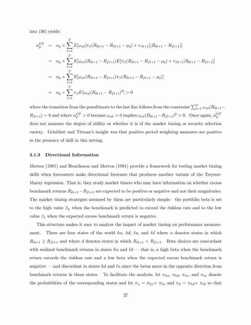
into (36) yields:
αGTp = αp +TXt=1
E[ωαt[πβ(Rδt+1 −Rft+1 − μδ) + υβt+1](Rδt+1 −Rft+1)]
= αp +TXt=1
E[ωαt(Rδt+1 −Rft+1)E[πβ(Rδt+1 −Rft+1 − μδ) + υβt+1|Rδt+1 −Rft+1]]
= αp +TXt=1
E[ωαt(Rδt+1 −Rft+1)πβ(Rδt+1 −Rft+1 − μδ)]
= αp +TXt=1
πβE[ωαt(Rδt+1 −Rft+1)2] > 0
where the transition from the penultimate to the last line follows from the constraintPT
t=1 ωαt(Rδt+1−
Rft+1) = 0 and where αGTp > 0 because ωαt > 0 implies ωαt(Rδt+1−Rft+1)2 > 0. Once again, αGTp
does not measure the degree of ability or whether it is of the market timing or security selection
variety. Grinblatt and Titman’s insight was that positive period weighting measures are positive
in the presence of skill in this setting.
3.1.3 Directional Information
Merton (1981) and Henriksson and Merton (1981) provide a framework for testing market timing
skills when forecasters make directional forecasts that produces another variant of the Treynor-
Mazuy regression. That is, they study market timers who may have information on whether excess
benchmark returns Rδt+1−Rft+1 are expected to be positive or negative and not their magnitudes.
The market timing strategies assumed by them are particularly simple: the portfolio beta is set
to the high value βh when the benchmark is predicted to exceed the riskless rate and to the low
value β when the expected excess benchmark return is negative.
This structure makes it easy to analyze the impact of market timing on performance measure-
ment. There are four states of the world hu, hd, u, and d where u denotes states in which
Rδt+1 ≥ Rft+1 and where d denotes states in which Rδt+1 < Rft+1. Beta choices are concordant
with realized benchmark returns in states hu and d – that is, a high beta when the benchmark
return exceeds the riskless rate and a low beta when the expected excess benchmark return is
negative – and discordant in states hd and u since the betas move in the opposite direction from
benchmark returns in these states. To facilitate the analysis, let πhu, πhd, π u, and π u denote
the probabilities of the corresponding states and let πu = πhu+ π u and πd = πhd+ π d so that
27

πu + πd = 1.
The managed portfolio return is still described by the conditional Jensen regression but the
model for portfolio betas takes a particularly simple form in this case. The conditional beta in
up markets is equal to βh with probabilityπhuπu
and equals β with probability π uπuwhile the down
market beta is equal to βh with probabilityπhdπdand equals β with probability π d
πd. Now consider
the regression of portfolio returns on both the up market excess benchmark return (Rδt+1−Rft+1)+
and the down market excess benchmark return (Rδt+1 −Rft+1)−:
Rpt+1 −Rft+1 = αp + β+p (Rδt+1 −Rft+1)+ + β−p (Rδt+1 −Rft+1)
− + εpt+1, (37)
where β+p and β−p are the up and down market portfolio betas, respectively. As is readily apparent,
the up and down market betas as well as the average beta are given by:
β+p =πhuπu
βh +π u
πuβ
β−p =πhdπd
βh +π d
πdβ (38)
βp = (πhu + πhd)βh + (π u + π d)β .
Moreover, the conditions under which the manager has market timing ability takes a particularly
simple form since:
β+p − βp =
∙πhuπu− (πhu + πhd)
¸βh +
∙π u
πu− (π u + π d)
¸β
= (1− πu)
∙πhuπu
+π d
πd− 1¸(βh − β ) (39)
is positive if and only if πhuπu+ π d
πd> 1 or, equivalently, if πhu
πu> πhd
πd. Since β−p − βp must be
negative if β+p − βp is positive, the covariance between betas and subsequent excess benchmark
returns is positive as well in this case and so only managers whose information and behavior is
such that πhuπu+ π d
πd> 1 possess market timing ability. This makes intuitive sense: the concordant
probabilities have to be larger than the discordant ones or betting on the up and down market
betas is a losing proposition. Note also that αp is the expected return to selection because the
covariance between betas and subsequent excess benchmark returns is embedded in the fitted part
of the regression.
This first version of this regression in Merton (1981) looks more like Treynor-Mazuy regres-
sion. Instead of having up and down market excess benchmark returns on the right hand side
28

as in (37), the regressors in the original model are Rδt+1 − Rft+1 and −(Rδt+1 − Rft+1)−. This
reparameterization of (37) is given by:
Rpt+1 −Rft+1 = αp + b1p(Rδt+1 −Rft+1)− b2p(Rδt+1 −Rft+1)− + εpt+1 (40)
which is related to (37) via:
Rpt+1 −Rft+1 = αp + β+p (Rδt+1 −Rft+1)+ + β−p (Rδt+1 −Rft+1)
− + εpt+1
= αp + β+p (Rδt+1 −Rft+1)+ + β+p (Rδt+1 −Rft+1)
−
−β+p (Rδt+1 −Rft+1)− + β−p (Rδt+1 −Rft+1)
− + εpt+1
= αp + β+p (Rδt+1 −Rft+1)− (β+p − β−p )(Rδt+1 −Rft+1)− + εpt+1. (41)
The expressions for β+p and β−p in (41) imply that b1p and b2p are given by:
b1p = β+p =πhuπu
βh +π u
πuβ
b2p = β+p − β−p =
∙πhuπu
+π d
πd− 1¸(βh − β ) (42)
and so b2p 6= 0 if and only if the manager possesses market timing ability. Merton (1981) provided
an elegant economic interpretation of b1p and b2p: b1p is the hedge ratio for replicating the option
with returns that are perfectly correlated with the returns to market timing and b2p is the implicit
number of free put options on the benchmark struck at the riskless rate that is generated by the
market timing ability of the manager.
3.2 Observable Information Signals
In the analysis so far the key variable is the timing signal, the variable that causes the manager
to bet on market direction. If we observed the signals themselves, we could separate the question
of whether the manager has forecasting ability – that is, whether πhuπu+ π d
πd> 1 – from that of
how it informs the manager’s trading strategy – that is, the uses to which the forecast is put. It
could be that some managers are good forecasters but are poor at executing appropriate trading
strategies or have other unknown motives for trade. Irrespective of the reason, studying the signals
or forecasts observed by the manager can be an interesting exercise. Bhattacharya and Pfleiderer
29

(1985) discuss conditions (including symmetry of the underlying conditional payoff distribution)
under which a principal can elicit the agent’s (fund manager’s) true information.
Henriksson and Merton (1981) propose a simple nonparametric method for evaluating prediction
signals. The states of the world are the same as outlined above – that is, hu, hd, u, and d –
but h and refer to positive and negative market timing signals, respectively, not high and low
betas. For the concordant pairs hu and d, πhuπu+ π d
πd= 1 if and only if the signal is of no value and
πhuπu+ π d
πd> 1 if it has positive value; as noted by Henriksson and Merton (1981) πhu
πu+ π d
πd< 1 also
has positive value in the perhaps unlikely event that one recognizes that the forecasts are perverse.
The adding up restrictions for up and down probabilities – that is, πu + πd = 1 – under the null
hypothesis of no market timing ability imply that πhuπu= πhd
πdand π u
πu= π d
πdor, in other words, that
the high and low signals are independent of whether ex post excess benchmark returns are positive
or negative.
Now consider a sample based on this implicit experiment: the 1’s and 0’s corresponding to
positive h signals and negative signals and those corresponding to whether the observed excess
benchmark returns are positive or negative. A sample of size T will then have Thu, Thd, T u, and T d
observations in the cells corresponding to each state of the world with T = Thu+Thd+T u+T d and
with Tu = Thu+T u and Td = Thd+T d observations in the up and down cells, respectively. Suppose
that returns are independently and identically distributed under the null hypothesis, a condition
that is a bit stronger than is necessary, so that the up and down probabilities are constant over
time. If the null is true, independent of the up and down probabilities, the sample proportions
respect:
πhuπu
= E
∙Thu
Thu + T u
¸= E
∙Thd
Thd + T d
¸=
πhdπd
= E
∙Thu + Thd
T
¸= πh.
Henriksson and Merton (1981) used this independence – that is, πhu = πhπu and πhd = πhπd
– to calculate the conditional probability of receiving one cell count from the other three. This
computation is facilitated by partitioning the sample into Thu, Th, Tu, and Td. Then the probability
30

of receiving Thu concordant up market pairs given the other three cell counts is given by:
Pr[Thu = Nhu|Tu, Td, Th] =Pr[Thu = Nhu, Th = Nh|Tu, Td]
Pr[Th = Nh|T ]
=Pr[Thu = Nhu, Thd = Nh −Nhu|Tu, Td]
Pr[Th = Nh|T ]
=Pr[Thu = Nhu|Tu]Pr[Thd = Nh −Nhu|Td]
Pr[Th = Nh|T ].
This holds because the high/low split is independent of the up/down split in the absence of
market timing ability. The reason for repartitioning the sample in this fashion is now obvious:
each probability is that of a binomial random variable with the same probability πh. Hence, the
probability is given by:
Pr[Thu = Nhu|Tu, Td, Th, πh] =Pr[Thu = Nhu|Tu, πh]Pr[Thd = Nh −Nhu|Td, πh]
Pr[Th = Nh|T, πh]
=
¡ TuThu
¢πThuh (1− πh)
Tu−Thu¡ TdTh−Thu
¢πTh−Thuh (1− πh)
Td−(Th−Thu)¡ TTh
¢πThh (1− πh)T−Th
=
¡ TuThu
¢¡ TdThd
¢¡ TTh
¢ =Th!T !Tu!Td!
Thu!T u!Thd!T d!T !(43)
independent of the high signal probability πh. The test is therefore distribution-free under the null
hypothesis so long as the up probability πu is constant. Henriksson and Merton (1981) point out
that this ratio follows a hypergeometric distribution, which makes sense because this distribution
is appropriate for experiments that differ in one detail for binomial experiments: a sample is first
drawn at random from some overall population without replacement and is then randomly sorted
into successes and failures. In this application, T is the size of the population, Th is the size of
the random sample, Thu is the number of successes, and Thd is the number of failures. Cumby and
Modest (1987) noted that the Henriksson/Merton test statistic is identical to Fisher’s exact test
for 2x2 contingency tables since:
prediction realization sum
Up Down
High Thu Thd Th
Low T u T d T
sum Tu Td T
They also noted that there is a convenient normal approximation to the test of the moment condition
31

E[ThuT −ThT
TuT ] = 0 that is given by:
Thu − ThT
TuTq
ThT TuTdT 2(T−1)
∼ N(0, 1) (44)
Pesaran and Timmermann (1992) show how to extend the analysis to more than two outcomes.
4 Performance Measurement and Attribution with Observable
Portfolio Weights
This state of affairs is somewhat unsatisfying and reflects the fact that returns are being asked to
do a lot of work. The theory is straightforward and beautiful: all marginal investors agree that
performance should be judged relative to portfolio δ, a specific conditionally mean-variance efficient
portfolio. Unfortunately, the identification of an empirical analogue of this portfolio is problematic
and it is likely that much of the evidence on fund performance reflects the inadequacy of benchmarks
and not the abilities of fund managers. Moreover and perhaps more importantly, fund returns are
being asked to tell us both the fund’s normal performance– that is, the appropriate expected return
given its normal exposure to risk – as well as any abnormal performance due to security selection
skill or market timing ability. In addition, the role played by parametric assumptions such as
normality in dealing with this problem is worrisome. In the absence of a priori information about
time-variation in expected benchmark returns and fund risk exposures, performance evaluation
based solely on fund and benchmark returns is simply not feasible. Performance evaluation is
somewhat less problematic when it is plausible to assume that risk exposures are constant a priori,
leaving benchmark error as the principle source of difficulty.
Of course, simplest of all is the case in which managers are judged on the basis of excess
returns over an explicit benchmark. It is noteworthy that compensation contracts are increasingly
taking this form and that managed portfolio performance is now routinely reported relative to an
explicit benchmark irrespective of the nature of the manager’s compensation. This change in best
practice is a very real measure of the considerable impact that the academic performance evaluation
literature has had on the portfolio management industry.
In fact, performance evaluation via the difference between the managed portfolio and benchmark
returns contains an implicit model of the division of labor between two hypothetical (and, often,
32

real) active portfolio managers: a market timer and a stock picker.10 The stock picker chooses
a portfolio of these N assets called δS which is structured to have a beta of one on δ because its
performance is measured relative to δ. That is, its return is given by:
RSδt+1 = Rδt+1 + αpt + εpt+1 (45)
where αpt = E[RSδt+1−Rδt+1|It] correctly measures the conditional expected excess return produced
by the stock picker. The quantity RSδt+1−Rδt+1 = αpt+εpt+1 is called the tracking error in portfolio
δS (with respect to its benchmark δ). The market timer takes this portfolio as given and determines
the fraction ωpt of the overall portfolio p that is allocated to portfolio δS at time t and the fraction
1− ωpt that is allocated to the riskless asset. Hence, the overall return on p is given by:
Rpt+1 = (1− ωpt)Rft+1 + ωptRSδt+1 (46)
We have a division of labor and a benchmark for evaluating the performance of one of the laborers.
What is missing is a benchmark for the market timer, a measure of normal performance for the
asset allocation choice. For simplicity, suppose that the normal or strategic asset allocation –
the passive portfolio that would be chosen by the manager of the overall portfolio in the absence
of attempts to time the market – is an allocation of ωnpt to portfolio δS and 1−ωnpt to the riskless
asset. Clearly any measure of the performance of the market timer should involve ωpt − ωnpt, the
market timer’s policy tool, and how it moves with benchmark returns.
Armed with this additional datum, the overall return to p can be rewritten as:
Rpt+1 = (1− ωpt)Rft+1 + wptRSδt+1
= Rft+1 + ωpt(RSδt+1 −Rft+1) (47)
= Rft+1 + ωnpt(RSδt+1 −Rft+1) + (ωpt − ωnpt)(R
Sδt+1 −Rft+1)
which is almost, but not quite, in a form suitable for assessing the performance of the market timer.
The missing element is the substitution of the return of the security selection portfolio δS into this
10Obviously, the more correct term here is ”asset picker” or ”security selector.” Both seem awkward and the phrase
stock picker is the term of art in the profession.
33

expression which yields:
Rpt+1 = Rft+1 + ωnpt(Rδt+1 + αpt + εpt+1 −Rft+1)
+(ωpt − ωnpt)(Rδt+1 + αpt + εpt+1 −Rft+1)
= [Rft+1 + ωnpt(Rδt+1 −Rft+1)] + ωnpt[αpt + εpt+1]
+[(ωpt − ωnpt)(Rδt+1 −Rft+1)] + [(ωpt − ωnpt)(αpt + εpt+1)] (48)
Note this expression is perfectly compatible with the conditional Jensen regression with βpt = ωpt,
ωptαpt equal to the conditional Jensen alpha, and ωptεpt+1 equal to the residual return. Note also
that observation of the portfolio weights ωpt and ωnpt are equivalent to observation of the conditional
and target betas, respectively, in these circumstances.
This simple portfolio arithmetic was introduced in Brinson et al. (1986) and provides a nearly
perfect decomposition of returns into economically relevant components. The first term in square
brackets is the normal portfolio return, the return on the portfolio in the absence of active man-
agement. The second term in square brackets is the return to security selection which is given by
the portfolio tracking error since the stock picker is measured relative to the benchmark portfolio
δ. The third term in square brackets is a natural measure of the performance of the market timer:
the product of ωpt−ωnpt, the deviation from the normal weight that is chosen by the manager, and
the excess return on the benchmark portfolio. The choice of the benchmark portfolio makes sense:
the use of δS would mix market timing ability with the security selection skill of the stock picker.
Of course, this ambiguity is merely pushed into the fourth term in square brackets: the product of
the asset allocation choice of the market timer ωpt − ωnpt and the tracking error of the stock picker
αpt + εpt+1.
This residual component (ωpt − ωnpt)(αpt + εpt+1) cannot be clearly assigned to either active
manager, which is why we termed this decomposition ”nearly perfect.” This circumstance arises
because the market timing portfolio is the stock picker’s portfolio δS , not the benchmark portfolio.
In fact, the residual would vanish if the tools of active management were modified so that the
market timer used the benchmark portfolio since the decomposition would be given by:
Rpt+1 = (1− ωpt)Rft+1 + ωnptRSδt+1 + (ωpt − ωnpt)(Rδt+1 −Rft+1)
= [Rft+1 + ωnpt(Rδt+1 −Rft+1)] + ωnpt[αpt + εpt+1] (49)
+[(ωpt − ωnpt)(Rδt+1 −Rft+1)]
34

which cleanly allocates overall return to strategic or normal asset allocation, security selection,
and market timing. Actual managed portfolios can use this decomposition when their market
timers use index futures markets to make market timing bets and the allocations to their stock
pickers are permitted to drift away from normal weights with infrequent reallocations when the
cumulative deviation grows sufficiently large. Of course, the residual will be small when the
allowable deviations from strategic asset allocations as well as the returns to security selection are
small, conditions that frequently obtain in actual practice.
Of course, the universe of assets is seldom broken down into only two asset classes or sectors.
The decomposition into J asset classes is straightforward:
Rpt+1 ≡JX
j=1
ωpjtRjt ≡JX
j=1
ωnpjtRnjt +JX
j=1
ωnpjt(Rjt −Rnjt) +
JXj=1
(ωpjt − ωnpjt)Rnjt +JXj=1
(ωpjt − ωnpjt)(Rjt −Rnjt) (50)
where ωpjt and ωnpjt are the actual and normal or strategic asset allocations of portfolio p, respec-
tively, and Rjt and Rnjt the corresponding actual and benchmark asset class returns. This relation
can be rewritten in the excess return form when the riskless asset, often termed cash in common
parlance, is one of the asset classes.
This decomposition of the performance of active managers into market timing and security
selection components across asset classes or sectors is called performance attribution and it is
now widely used in actual practice. This division of labor also roughly reflects the management
structure at many, if not most, large pension funds, although the market timing or tactical asset
allocation is often done passively. Their investment policy statements typically carve up the asset
menu into a number of asset classes and choose explicit benchmarks against which asset class
returns are measured with no beta adjustment, corresponding to a structure in which asset class
managers are hired and instructed to remain fully invested in the asset class since their performance
will be measured against the asset-class-specific benchmark. Moreover, they often specify both
the normal or strategic asset allocation weights and the permissible amounts by which the actual
asset allocations are allowed to deviate from the normal ones, which corresponds to a short run
or tactical asset allocation manager (or managers) who choose asset class exposures and who sit
one level above the asset class managers. In addition, it is now common for fiduciaries to read
performance attribution reports that make routine reference to tracking errors and risk exposures.
35

It is fair to say that performance measurement and attribution along these lines is one of the many
dimensions in which financial economics has had an effect, and a beneficial one at that, on real
world investment practice.
Note that there is an implicit assumption about the investment opportunity set in this man-
agement structure. Asset class managers can look at correlations within asset classes and market
timers can consider comovements across benchmarks but neither has the incentive to consider
the covariances between each asset class benchmark and individual security returns in other asset
classes. In fact, they have a disincentive to do so because they are typically rewarded according
to benchmarks that make no provision for such correlations. Hence, it is imperative that the asset
class definitions be narrow enough so that the fund does not unintentionally overlook valuable
diversification opportunities. Put differently, carving up the asset menu into asset classes with
specific benchmarks creates another potential source of benchmark error when:
Rδt+1 −Rft+1 6=JXj=1
ωnpjtRnjt (51)
While we are unaware of any empirical evidence on this question, a cursory examination of the
investment policy statements of large public US pension funds suggests that such breakdowns are
quite refined and probably do not result in materially inferior diversification.
The extent to which performance attribution can be usefully employed depends on whether one
is viewing the portfolio from inside the fund or from the outside. Clearly, this method cannot
be used without information on actual and normal or strategic asset allocations along with actual
and benchmark asset class returns. Data on all of these quantities can be obtained within the
fund when it has an explicit investment policy governing asset allocation and benchmarks. The
academic perspective, however, is typically external to the fund and so which of these data are
available hinges on what has been reported to the data source. Actual and benchmark asset class
returns along with the actual allocation were available in the two main academic applications of
these tools, Brinson et al. (1986, 1991), who studied US pension funds, and Blake, Lehmann and
Timmermann (1999), who examined UK pension funds. Neither study had data on normal or
strategic asset allocations.
While our emphasis is on methods and not on empirical evidence, there are two results that are
both quite striking and of great relevance for performance measurement and attribution. The first
concerns the extent to which performance measurement based on tracking error results in managers
36

actually setting betas equal to one. Lakonishok, Shleifer, and Vishny (1992) found sample equity
betas to be tightly clustered about one – raw beta estimates and not betas significantly different
from one at some significance level – in a sample of US pension fund stock portfolios and Blake
et al. (1999) found similar results for their sample of UK pension funds. That is, managers
typically have the incentive to set betas to one and the evidence suggests that they are good at
doing so. The second broad result concerns market timing. Brinson et al. (1986) found that only
one out of the 96 U. S. pension funds they studied had positive – not statistically significant at
some confidence level but simply positive – market timing measures. Similarly, Blake et al (1999)
found that roughly 80 per cent of the 306 UK pension funds they examined had negative market
timing measures with the average return from market timing (at -34 basis points per annum) was
statistically significant. Put differently, pension fund managers have typically attempted to time
the overall market or individual asset class returns but they have been unsuccessful in doing so.
This last observation has had a profound impact on beliefs about the extent to which managed
portfolios benefit from market timing. Many pension funds now follow the passive market timing
strategy based on mechanical rebalancing rules, letting their asset class managers – that is, those
engaged in security selection – implicitly choose increased pension fund exposure to asset classes
when they outperform their benchmarks and lower exposures after underperformance. Other
pension funds manage their ”traditional” assets this way but buy explicit market timing services
from hedge funds, with performance being measured against Treasury bills. That is, a generation
of pension fund investment consultants have used this evidence to persuade their clients to forego
market timing or to treat it as an asset class with a strict performance standard.
In any event, external performance measurement and attribution with data on actual asset
allocations along with actual and benchmark asset class returns requires a model for the strategic
or normal asset allocation. Brinson et al. (1986) use sample averages of portfolio weights as the
normal portfolio weights:
ωnpjt = ωnpj =TXt=1
ωpjt/T (52)
which is a reasonable definition if the fund has a stable de facto asset allocation. However, asset
allocations that drift in a particular direction as was the case in the UK pension funds by Blake et
al. (1999) makes this assumption untenable. The models they explored include a linear trend in
37

normal portfolio weights:
ωnpjt = ωpj1 + (t/T )(ωpjT − ωpj1), (53)
identical strategic asset allocations across funds at a point in time:
ωnpjt =PXp=1
ωnpjt, (54)
where P is the number of pension funds in the sample, which implicitly assumes zero timing ability
for the funds as a whole.11
Returning for simplicity to the case of two assets, recall that the portfolio weights wpt and wnpt
are equal to the conditional and target betas, respectively, of a portfolio managed in this fashion.
This observation suggests that tests for the presence of market timing ability can be based on the
conditional and unconditional projections (24) and (28). Consider first the baseline case in which
both ωpt and ωnpt are observed for a particular asset class so that ξβpt = βpt− βpt = ωpt − ωnpt.
Since ξβpt is the innovation in the conditional portfolio beta given publicly available information
(i.e., E[ξβpt |It] = 0), the projection of benchmark returns on ξβpt is given by:
Rδt+1 −Rft+1 = π0 + πpξβpt + υδt+1 (55)
πp 6= 0 if and only if the manager possesses market timing ability in great generality. In partic-
ular, benchmark excess returns can have arbitrary serial dependence so long as it does not affect
the ability of least squares to estimate πp consistently.12 This is an obvious consequence of the
assumption that both βpt and βpt are observed via ωpt and ωnpt.
Of course, we typically observe ωpt but not ωnpt which corresponds to observations on βpt but
not on βpt and, hence, not on ξβpt . The unobservability of ωnpt is a subtle problem because its
11Other alternatives are the error components model used to summarize the stochastic properties of asset class
weights in Blake et al. (1999) and the asset allocation guidelines of the funds with public investment policy statements.
Neither approach has been tried in the literature to the best of our knowledge.
12The residual in this projection inherits the serial corrrelation properties of excess benchmark returns. That is:
E[υδt+1|It] = E[Rδt+1 −Rft+1|It]− π0 = μδt − μδ
which would typically be assumed to be well-behaved. Typical bounds on higher order dependence would then yield
consistency of least squares in this application.
38

strategic nature suggests that most of its fluctuations occur at low frequencies. That is, πp in (55)
is given by:
πp =Cov(μδt, βpt + ξβpt)
V ar[βpt]+
E[(Rδt+1 −Rft+1 − μδt)(βpt + ξβpt)]
V ar[βpt]
=Cov(μδt, βpt)
V ar[βpt]+
Cov(Rδt+1 −Rft+1, ξβpt)
V ar[βpt](56)
The first term is the bias due to predictability of benchmark returns and the absence of observations
on βpt while the second term is nonzero if and only if market timing is present. Note that only the
conditional first moment of excess benchmark returns (and not higher moments) is relevant here,
one of the benefits of the observability of βpt under these assumptions.
As in our earlier discussion of the Treynor-Mazuy regressions, there are three approaches to
dealing with the bias term in this regression. The first is to assume it away via constancy of μδt
and/or βpt or Cov£μδt, βpt
¤= 0. Alternatively, one can postulate a model for μδt and rewrite
(55) in terms of Rδt+1 − Rft+1 − μδt, which requires model errors – that is, nonzero values of
E[Rδt+1 − Rft+1 − μδt|It] – to be uncorrelated with βpt. Finally, one can postulate a model for
the target beta βpt = f(zt, θ), where zt ∈ It is publicly available conditioning information and θ is
a vector of unknown parameters that can be estimated consistently since consistent estimation of
βpt implies consistent estimation of ξβpt .13
Graham and Harvey (1996) adopt a variant of this last approach which works instead with
changes in actual asset allocations and zt as additional regressors as in:
Rδt+1 −Rft+1 = π∗0z zt + π∗p4ωpt + υ∗δt+1
where a test of the hypothesis π∗p = 0 is a test of the hypothesis that portfolio weight changes
Granger-cause (i.e., predict) benchmark excess returns. This projection is conveniently analyzed
by considering the two unconditional population projections:
μδt = φ0δzt + eδt,
βpt − βpt−1 − ξβpt−1 = φ0wzt + ewt
13Note that this last approach requires that f(zt, θ) be incorporated in (55) in the restricted fashion:
Rδt+1 −Rft+1 = π0 + πp[ωpt − f(zt, θ)] + υδt+1
if the goal is to mimic (55) exactly because the required regressor is ξβpt . However, the natural desire to correct for
serial correlation in υδt+1 would normally militate in favor of including zt or suitable functions of zt as regressors.
39

since:
π∗p =Cov(Rδt+1 −Rft+1 −φ0δzt,4ωpt − φ0wzt)
V ar[4ωpt − φ0wzt]
=Cov[μδt − φ0δzt,4βpt − ξβpt−1 − φ
0wzt] + Cov(Rδt+1 −Rft+1, ξβpt)
V ar[ξβpt + ewt]
=Cov[eδt, ewt]
V ar[σ2ξ + σ2ew ]+
Cov(Rδt+1 −Rft+1, ξβpt)
σ2ξ + σ2ew, (57)
where the bias term depends on the correlation of the projection errors. A priori confidence in
the merits of this specification involves a belief that the bias is small and that 4βpt is close to an
innovation sequence, thus mitigating the main source of serial correlation in this specification.
Another test of market timing when portfolio weights are observed is suggested by the Henriks-
son and Merton (1981) analysis of the fidelity between signals and outcomes given at the end of
the previous section. An interesting special case is that of tactical asset allocation in which the
manager allocates 100% to the benchmark portfolio when placing an up market bet and 100% to
the riskless asset when placing a down market bet. This corresponds to setting βh = 1 and β = 0
and with up, down, and expected betas of β+p =πhuπu, β−p =
πhdπd, and βp = πh, respectively. Accord-
ingly, evaluating the performance of tactical asset allocation with observable portfolio weights that
only take on the values one and zero is equivalent to the evaluation of prediction signals given in
the previous section. Hence, inference for the hypothesis πhuπu+ π d
πd= 1⇔ πhu
πu= πhd
πdcan proceed
based on the hypergeometric distribution while that for the hypothesis πhu = πhπu can be based
on the asymptotic normal approximation.
More generally, we can use observed portfolio weights to implicitly evaluate the fidelity of market
timing signals using the Henriksson-Merton approach. If we assume that up and down markets
have constant probabilities and that the manager has a constant target beta, ωpt − ωp will be
perfectly correlated with the signal since the manager will have a beta above the mean – that is,
βpt > βp – in the high signal state and one below the mean in the low market state. When the
strategic asset allocation and, hence, the target beta is observed, which is possible in some cases
through examination of investment policy statements, the cell counts can be based on the sign of
ωpt − ωp and inference can be based on can be the hypergeometric distribution (43). If it is not,
the cell counts can be based on the sign of ωpt − ωp, where ωp = 1T
PTt=1 ωpt, and inference can be
based on the normal approximation (44) since ωp → ωp in probability in great generality.
Grinblatt and Titman (1993) implement period weighting measures when portfolio weights are
40

observed under the assumption that uninformed investors perceive expected asset returns to be
constant over time and returns to be independently and identically distributed. In this circum-
stance, changes in portfolio weights should not be correlated with future returns. In contrast,
informed investors will adjust portfolio weights in anticipation of future returns and, if their infor-
mation is valid, portfolio weight changes should be correlated with future returns. The exact form
of the relation will depend on the way in which the informed investor’s information and preferences
interact to produce a portfolio decision rule. That said, the unconditional covariance between
portfolio weights and future returns should be positive under the weak assumption that portfolio
weights are increasing in each asset’s conditionally expected return. A simple test for the presence
of performance ability can be based on the sum of the covariances between portfolio weights and
asset returns across all assets in the universe:
cov =NXj=1
(E[ωjRj ]−E[ωj ]E[Rj ]). (58)
This is equal to the expected return of the investor’s actual portfolio minus the expected return if
portfolio weights and returns were uncorrelated. The second term also acts as a risk-adjustment
since it gives the expected return on a portfolio with the same average risk as the actual portfolio.
Equation (58) can equivalently be rewritten in two ways:
cov =NXj=1
E[ωj(Rj −E[Rj ])] (59)
or
cov =NXj=1
E[(ωj −E[ωj ])Rj ]. (60)
Since ωj and Rj are observed, these expressions point to two types of additional information that
can be used to produce period weighting measure estimates described in the previous section.
The first of these expressions (59) requires an estimate of the (unconditional) expected return,
E[Rj ]. Given the assumption that returns are identically and independently distributed, a natural
way to proceed is to use average future returns on these assets, making this approach much like an
event study in that returns from outside the event window − the performance measurement period
in this case − measure normal performance. Abnormal performance arises when these assets earn
higher returns when they are in the investor’s portfolio than at other times.
The second expression (60) requires instead an estimate of the expected portfolio weight ωj .
This formulation is more problematic because serial dependence in weights − such as that produced,
41

for example, by momentum or contrarian investment strategies − causes sample period weighting
measures to be biased. If the serial dependence in momentum or contrarian portfolio weights is
short-lived, such biases can be mitigated or eliminated by introducing a lag between return and
expected portfolio weight measurement. For example, if weights are covariance stationary, each
observed weight is an unbiased estimate of expected portfolio weights. If weights and returns are
K dependent − that is, if they are independent when K periods separate their measurement −
there is no such bias. Hence, Grinblatt and Titman (1993) recommend setting E[ωj ] = ωjt−K ,
resulting in period weighting estimates of the form:
ccovω = 1
T
NXj=1
TXt=K
(ωjt − ωjt−K)Rjt,
and they use the same idea for expected returns by setting E[Rj ] = Rjt+K in the revised estimate:
ccovR = 1
T
NXj=1
T−KXt=1
ωjt(Rjt −Rjt+K),
Each of these measures will converge to zero provided fund managers use no information with
predictive content regarding future returns when setting their portfolio weights and returns are not
predictable for uninformed investors. That said, ccovω makes for simpler inference than ccovR, sinceits returns are serially uncorrelated when individual asset returns are serially uncorrelated as well.
In contradistinction, the overlapping returns implicit in ccovR make its returns K − 1 dependentwhen individual asset returns are serially uncorrelated. Hence, the test statistic based on ccovω isa simple test of the null hypothesis that a mean is zero.
4.1 Should investors hold mutual funds?
A key question from an investor’s point of view is whether−and how much−to invest in one or more
mutual funds. Suppose that we cannot reject the null hypothesis that a particular fund’s alpha
equals zero although its point estimate indicates a sizeable skill level. This is a likely empirical
outcome due to the weak power of these tests. Does this mean that the investor should not invest
in this mutual fund? Clearly this is not implied by the outcome of the statistical test, which is
typically based on a discrete loss function that is typically very different from the underlying utility
function. Statistical tests do not in general trade off the cost of wrongly including an investment
42

in a mutual fund versus wrongly excluding it.14 Conversely, suppose we reject the null that the
portfolio weight on the mutual fund(s) equals zero, then how much should be invested in such
funds?
The investor’s decision of whether to hold mutual funds at all is naturally set up as a test on the
portfolio weights when data on these are available. When investors have mean-variance preferences,
constructing such a test and deriving its properties is quite straightforward and can be based on
a simple regression approach to portfolio selection that minimizes the squared deviations between
the excess returns on a constructed portfolio and the excess returns implicit in the unity vector,
ι, cf. Britten-Jones (1999). This minimization can be implemented through a projection of ι on
excess returns on the risky assets and mutual funds, excluding an intercept term. To this end,
define the N + P−vector of period-t+ 1 excess return on all risky assets extended to include a set
of P mutual funds as ert+1= (R0t+1 R0pt+1)0 − ιRft+1, and let er= (r1 r2 · · · rT )0 be the T × (N + P )
matrix of stacked returns, where the ‘tilde’ on top of the vector of excess returns indicates that
we are referring to the original set of assets extended to include returns on the mutual funds. The
projection proposed by Britten-Jones is
ι = erβ + u. (61)
The resulting vector of estimated coefficients,
b = (er0er)−1er0ι, (62)
gives − up to a proportionality factor − the weights of the mean-variance efficient portfolio of risky
assets. Using the scaling b/ι0b, we get the maximum Sharpe ratio (tangency) portfolio:
Σ−1r
10Σ−1r
where r = er0ι/T is the sample mean while the (maximum likelihood) sample covariance matrix is
Σ = (er− 1r0)0(er− 1r0)/T .Suppose that there are P mutual funds under consideration (the last P assets in the vector of
excess returns, er). Then the restriction that the investor should entirely exclude mutual funds from14Although in principle one could make the critical level used to define the nominal size of the statistical test a
function of the relative cost of type I and type II errors, this does not resolve the problem that the hypothesis testing
uses a discrete decision, whereas the investor’s utility function is generally assumed to be continuous.
43

the portfolio takes the form
Γb = 0,
where the P × (N + P ) matrix of restrictions, Γ, is given by
Γ =³0P×N IP
´.
Assuming that returns are joint normally distributed and independently and identically distributed,
this restriction can be tested through the F -statistic
(SSRr − SSRu)/P
SSRu/(T −N − P ), (63)
where SSRu is the sum of squared residuals implied by the unrestricted regression underlying the
coefficient estimates in (62), SSRr is the sum of squared residuals from estimation of regression
(62) subject to the restriction that Γb = 0. This test statistic has an exact central F distribution
with P and T − N − P degrees of freedom. Under less restrictive distributional assumptions, a
method of moments type test can be used instead.
This framework lends itself to testing other economically interesting hypotheses. In particular
it can be used to testing whether a portfolio of the managed funds spans the asset menu by testing
if the weights on the non-mutual funds are jointly zero. We are unaware of any research in which
this role for managed portfolios has been examined.
4.2 Determining the optimal holdings in mutual funds
When preferences outside the mean-variance class are considered and we are also interested in
answering the second question − namely how much to invest in mutual funds − a more general
approach is called for. We illustrate a simple method valid in a single-period setting where dynamic
programming concerns can be ignored. Let Wt,Wt+1 be an investor’s current and future wealth
and suppose that the investor evaluates utility from future wealth through the function U(Wt+1).
Returns on traded risky assets and mutual funds are again given by eRt+1=(R0t+1 R
0pt+1)
0, whileeωt = (ω0t ω
0pt)0 is the associated vector of portfolio holdings. Future wealth associated with a given
set of portfolio holdings is simply
Wt+1 =Wt(eω0t eRt+1),
44

while the investor’s optimization problem is to maximize expected utility conditional on current
information, It :
maxωt
E[U(Wt(eω0t eRt+1))|It].
The portfolio weights on the mutual funds can be obtained from the last P elements of eωt corre-
sponding to the mutual fund returns.
For example, in the earlier example with mean-variance preferences,
E[U(Wt+1)|It] = E[Wt+1|It]−γ
2V ar(Wt+1|It),
where γ is the absolute risk aversion. This gives a closed-form solution (cf. Ait-Sahalia and Brandt
(2001)): eωt = Σ−1t ι
γWt − ι0Σ−1t μt
γWtι0Σ−1t ι
+Σ−1t μt
γWt,
where Σt = V ar(eRt+1|It) and μt = E(eRt+1|It). Since (conditional) population moments are
unknown, in practice sample estimates of these moments, Σ and μ, are typically plugged in to get
estimated weights as follows:
ωt = Σ−1t ι
γWt − ι0Σ−1t μt
γWtι0Σ−1t ι
+Σ−1t μt
γWt.
This of course ignores the sampling errors in the moment estimates. Furthermore, due to the
nonlinearity in the mapping from Σ and μ to ωt, it is not possible to identify which predictors
zt ∈ It are important to portfolio holdings by inspecting the predictability of the mean and variance
of returns.
Rather than adopting a two-stage approach that first estimates a model for the predictive
distribution of returns and then plugs in the resulting parameter estimates in the equation for the
optimal weight, one can directly model the portfolio weights as a function of the predictor (or state)
variables, zt. To this end let the portfolio policy function map zt into optimal asset holdings:
eωt = ω(zt). (64)
Of course, in general both the functional form of the optimal portfolio policy ω(zt) and the form
of the predictability of returns are unknown. One way to deal with this that avoids the curse of
dimensionality is to follow Ait-Sahalia and Brandt (2001) and assume that the portfolio policy only
45

depends on the state variables through a single index, zt0β:
maxωt
E[U(Wt(eω0t eRt+1))|z0tβ],eωt = ω(zt0β;β)
This is a semiparametric approach that assumes a parametric (linear) index function but allows for
a flexible (non-parametric) policy function.
Differentiating the optimization problem with respect to eωt and using eωt = ω(X 0tβ;β) gives the
conditional moment condition
E[Qt+1(β)|zt] = E[U 0(Wt(ω(z0tβ;β)
0 eRt+1))eRt+1|z0tβ] = 0.
This can be estimated by GMM, using instruments g(zt) and the associated unconditional moment
conditions arising from
minβ
E[Qt+1(β)⊗g(zt)]0WE[Qt+1(β)⊗g(zt)]
where W = Cov(Qt+1 ⊗ g(zt))−1 is again some weighting matrix.
Alternatively, one can approximate the policy function, (64), using a series expansion such as
eωit = eω0i + nzXj=1
eω1ijzjt + nzXj=1
nzXk=1
eω2ijkzjtzkt, (65)
where nz is the number of z−variables. Again the parameters of the policy function can be estimated
using GMM.
5 The Cross-Section of Managed Portfolio Returns
What makes the econometrics of performance measurement and its economic setting different from
that of conventional asset pricing? As we noted earlier, Jensen’s alpha is just mispricing in asset
pricing models and the two settings share many econometric issues. The answer we pointed to is the
difference in the nature of the asset menu: individual securities or particular portfolios chosen by
the econometrician in the asset pricing case and managed portfolios in performance measurement
and attribution. These pages have been literally littered with examples of ways in which the direct
impact of investment choices of portfolio managers makes concerns like stochastic betas and the
measurement of biases in alphas first order concerns.
46

The other main difference is in the interpretation of rejections of the null hypothesis: researchers
often interpret rejections of the null for managed portfolios as a reflection of managerial skill while
rejections of the null in asset pricing theory tests are typically attributed to failures of the model.
Most papers that evaluate the performance of managed portfolios simply do not treat the finding
of economically and statistically significant alphas as an indication that the benchmark is not
conditionally mean-variance efficient. Most papers that evaluate the performance of asset pricing
models simply do not treat the finding of economically and statistically significant alphas as an
indication that the test assets are underpriced or overpriced.
What makes the stochastic properties of this universe of test assets different from the passive
− that is, unmanaged − portfolios typically employed in asset pricing theory tests? The answer
probably lies in the commonalities among portfolio managers arising from the comparatively small
range of investment styles and asset classes into which the universe of securities is partitioned.
The portfolios used in asset pricing theory tests are formed according to different principles. In
some cases, researchers seek dispersion across population conditional betas to facilitate more precise
estimation of any risk premiums, which reflects a concern for inferences about the implications of
the model under the null hypothesis that it is true. Many tests are based on portfolios formed on
the basis of security characteristics that proved to be correlated with the alphas from earlier asset
pricing models, reflecting a concern for inference when the null hypothesis is false. Others are
based on portfolios chosen because the underlying test assets were thought to have low correlation
conditional on the benchmark in question: industry and commodity portfolios have been chosen
for this reason at different times.
The commonalities among the trading strategies of portfolio managers make for potential dif-
ferences in each of these dimensions. The dispersion of conditional betas across funds is quite
small, probably because performance is typically measured relative to similar explicit or implicit
benchmarks which gives the managers strong incentives to maintain betas that are close to one.
Management styles are often highly correlated with security attributes as well and so managers have
to take bets that are different from the characteristics portfolios used by financial econometricians
in order to justify management fees. Finally, the very commonalities among trading strategies
suggest that residual correlations are likely to be higher in the managed portfolio setting than in
asset pricing theory tests. Of these, the second observation is likely to be second order but the
first and third are of first order importance.
47

5.1 Inference in the Absence of Performance Ability
Consider first the setting in which it is known a priori that the excess returns of N securities are
independently and identically distributed over time from the perspective of uninformed investors.
As before, let portfolio δ be the mean variance efficient portfolio based on these N assets. Portfolio
δ has constant weights under these assumptions and its excess returns are given by:
Rt+1 − ιRft+1 = βδ(Rδt+1 − ιRft+1) + εδt+1
where E[εδt+1|It] = 0.
Managers, however, need not have portfolio weights that are constant and the extent and
manner in which their weights vary over time depend on whether they believe they have skill at
market timing or security selection. Managers who do not believe they have market timing ability
but who think they possess skill at selection will tend to choose fixed weight portfolios if they
believe there are constant expected returns to selection but will have portfolios with time-varying
weights if they believe that the returns to selection varies across stocks over time.15 In terms of
the conditional Jensen regression, these managers will choose time-invariant betas and will believe
they have time-varying Jensen alphas. Managers who believe they have market timing ability will
also generically vary their weights over time so that their betas and, if they have skill at selection,
their alphas will vary over time as well.
Only tests of the skill of managers of the first kind – those with no timing ability and who know
it but who falsely think they possess skill at security selection with constant expected returns –
are completely straightforward in these circumstances. Such managers believe that their portfolios
satisfy the Jensen regression with constant conditional betas:
Rpt+1 −Rft+1 = αp + βp(Rδt+1 −Rft+1) + pt+1 (66)
where the manager believes that αp = E[ω0pεδt+1|Ipt] = ω0pE[εδt+1|Ipt] and the residual pt+1 =
ω0pεδt+1 is homoskedastic. Hence, the null hypothesis that the manager of portfolio p does not have
skill at selection can be tested with the simple t-test, which goes by the name of the Treynor-Black
appraisal ratio in the performance evaluation literature as was noted earlier.15As stated, this is somewhat of an oversimplification: constant expected returns to selection is not the same as
constant alphas security by security which is implicitly assumed by the statement. Moreover, constant expected
returns to selection will not lead to fixed weight portfolios if managers have implicit hedging demands, such as those
that can arise from different compensation schemes.
48

Similarly, a joint test that P such funds have skill at selection involves the P regressions:
Rpt+1 − ιRft+1 = αp + βp(Rδt+1 − ιRft+1) + ²pt+1
where the natural null hypothesis is:
H0 : αp = 0. (67)
If returns are normally distributed, this hypothesis can be tested via:
T (T − P − 1)P (T − 2)
α0pS−1pαp
1 + φ2δ
∼ F (P, T − P − 1).
where αp, S p is the sample covariance matrix of the residuals, and φ2δ is the sample squared Sharpe
ratio of the benchmark portfolio that is given by φδ =Rδ−Rf
sδwhere Rδ −Rf =
PTt=1(Rδt+1 −
Rft+1)/T and s2δ =PT
t=1(Rδt+1−Rft+1)2/(T −1)−
¡Rδ −Rf
¢2are the sample mean and variance
of benchmark returns, respectively. Jobson and Korkie (1982) and Gibbons, Ross and Shanken
(1989) showed that this statistic follows an exact F-distribution with P numerator and T − P − 1
denominator degrees of freedom. In large samples, we can dispense with normality since the
statistic:
Tα0pS
−1pαp
1 + φ2δ
∼ χ2(P ), (68)
is distributed as χ2 with P degrees of freedom asymptotically, although it is common to use the
associated F-statistic formulation as a sort of ad hoc small sample correction. This is a conventional
mean variance efficiency test where the test assets are managed portfolios.
Managers might believe they do not have timing ability but that they possess time varying
selection skill. Such managers will generically choose portfolios with time varying weights and
they will believe that their returns satisfy:
Rpt+1 −Rft+1 = ω0pt(Rt+1 − ιRft+1) = ω0ptβδ(Rδt+1 − ιRft+1) + ω0ptεδt+1
= αp + βp(Rδt+1 − ιRft+1) + αpt − αp + εpt+1
≡ αp + βp(Rδt+1 − ιRft+1) + pt+1
where the manager believes αpt = E[ω0ptεδt+1|Ipt] = ω0ptE[εδt+1|Ipt] 6= 0. If the manager is right,
αpt > 0, αp = E[αpt] > 0, and pt+1 = ω0ptεδt+1 is a heteroskedastic and serially correlated error
term. If the manager is wrong, αpt = αp = 0 and pt+1 = ω0ptεδt+1 is generically a heteroskedastic
and serially dependent, but not serially correlated, error term.
49

The principles governing hypothesis testing is a bit different under the null hypothesis of no
skill at security selection. The least squares estimate αp is given by:
αp = αp +1 + φ
2δ
T
TXt=1
pt+1 −Rδ −Rf
T
TXt=1
(Rδt+1 −Rft+1) pt+1 (69)
and, since εδt+1 is independently and identically distributed, its variance converges to:
V ar(αp) →1
T(1 + φ2δ)
2E[ 2pt+1]− 2(1 + φ2δ)Rδ −RfE[(Rδt+1 −Rft+1)2pt+1]
+Rδ −Rf2E[(Rδt+1 −Rft+1)
2 2pt+1] (70)
which obviously depends on the extent to which 2pt+1 = (ω
0ptεδt+1)
2 is related to Rδt+1 − Rft+1
and (Rδt+1−Rft+1)2. This is, of course, the familiar heteroskedasticity consistent estimator of the
variance of V ar(αp). If the portfolio weights are independent of market conditions, the variance
simplifies to:
V ar(αp)→(1 + φ2δ)
2σ2p
T
just as it did in the conditionally homoskedastic case and so inference can be based on the large
sample χ2−statistic (68), since normality of asset returns does not deliver normally distributed
managed portfolio returns when weights are time-varying.
As it happens, the case in which managers believe they have time-varying security selection
skill is identical to that in which they believe they have market timing ability when they do not
possess skill in either dimension. That is, the Jensen residual when managers feel they have both
market timing and stock picking ability is given by:
pt+1 = αpt − αp + (βpt − βp)(Rδt+1 −Rft+1) + εpt+1
where E[αpt−αp] = E[(βpt−βp)(Rδt+1−Rft+1)] = 0 under the null hypothesis. Hence, irrespective
of whether conditional heteroskedasticity arises from attempts at selection that are dependent on
market conditions or attempts at market timing, the joint hypothesis that P alphas are zero can
be tested χ2 statistic:
Tα0pS
∗pαp
1 + φ2δ
∼ χ2(P ) (71)
where S∗pis given by:
S∗p=
1
T
h(1 + φ2δ)
2S p − 2(1 + φ2δ)Rδ −Rf SRδ p +Rδ −Rf2SR2δ p
iSRδ p =
1
T
TXt=1
(Rδt+1 −Rft+1)ˆpt+10pt+1; SR2δ p
=1
T
TXt=1
(Rδt+1 −Rft+1)2²pt+1²
0pt+1
50

which makes S∗pthe heteroskedasticity consistent equivalent of S p .
Little is changed if we dispense with the assumption that returns are identically distributed
over time while maintaining the assumption of serial independence. From the perspective of the
Jensen regression, there is one more potential source of conditional heteroskedasticity related to
market conditions if returns are not identically distributed unconditionally. For this reason, too,
it would appear that conservative inference suggests the use of the heteroskedastic consistent χ2
statistic (71).
Serial dependence in returns from the perspective of uninformed investors can create additional
complexities. It need not do so: changes in betas due to time-variation in expected returns do
not bias Jensen alphas unless Cov[βpt, Rδt+1−Rft+1] = E[ςβptμδt] 6= 0 where βpt = βp+ ςβpt is the
conditional beta based on public information, not on market timing ability. Unfortunately, any
beta change of the form ςβpt = k(μδt − μδ) will cause this assumption to fail, biasing the Jensen
alpha upward on the natural hypothesis k > 0.
One general strategy for dealing with this problem is to attempt to measure ςβpt or, more
precisely, that portion of ςβpt that is correlated with expected benchmark returns μδt. To this end,
Ferson and Schadt (1996) propose modeling time variation in mutual fund betas as projections
onto observed conditioning information as in:
βpt = βp + π0β(zpt − μz) + eβt
where the identifying assumption is that:
E[eβt(Rδt+1 −Rft+1)] = E[eβt(Rδt+1 −Rft+1)] = 0
and so the alpha from the revised Jensen regression:
E[Rpt+1 −Rft+1 = αp + βp(Rδt+1 −Rft+1) + π0β(zpt − μz)(Rδt+1 −Rft+1) + pt+1
is purged of the effects of time variation in conditional benchmark betas related to public informa-
tion under these assumptions. Hence, this model can be estimated by ordinary least squares and
the inference procedures identified above can be applied to them without modification.
The Treynor-Mazuy regression coupled with the same sorts of simplifying assumptions provides
another avenue for dealing with serial dependence. As is obvious, this resolution can work here
51

because there is no timing ability under the null hypothesis. Accordingly, consider the Treynor-
Mazuy quadratic regression:
Rpt+1 −Rft+1 = ap + b0p(Rδt+1 −Rft+1) + b1p(Rδt+1 −Rft+1)2 + ζpt+1
along with the unconditional population projection:
Rδt+1 −Rft+1 = μδ + πςςβpt + υςδt+1 (72)
where the residual υςδt+1 is purged of the correlation of ςβpt with expected excess benchmark returns.
Now assume that excess benchmark returns Rδt+1−Rft+1 and beta innovations ςβpt are jointly nor-
mally distributed and strengthen the lack of correlation between υςδt+1 and ςβpt to independence.16
Substitution of (72) into the normal equations of this variant of the quadratic regression reveals
that the unconditional projection coefficients b0p and b1p are given by:⎛⎝ b0p
b1p
⎞⎠ =
⎡⎣V ar⎛⎝ Rδt+1 −Rft+1
(Rδt+1 −Rft+1)2
⎞⎠⎤⎦−1Cov⎡⎣Rpt+1 −Rft+1,
⎛⎝ Rδt+1 −Rft+1
(Rδt+1 −Rft+1)2
⎞⎠⎤⎦=
⎛⎝ σ2δ 0
0 3σ4δ
⎞⎠−1Cov⎡⎣(βp + ςβpt)(Rδt+1 −Rft+1) + pt+1,
⎛⎝ Rδt+1 −Rft+1
(Rδt+1 −Rft+1)2
⎞⎠⎤⎦=
⎛⎝ βp
0
⎞⎠+E
⎛⎝ ςβpt(μδ + πςςβpt + υςδt+1)(πςςβpt + υςδt+1)
ςβpt(μδ + πςςβpt + υςδt+1)[(πςςβpt + υςδt+1)2 − σ2δ ]
⎞⎠=
⎛⎝ βp
0
⎞⎠+ πςσ2ξ
σ2δ
⎛⎝ μδ23
⎞⎠ ≡⎛⎝ βp
0
⎞⎠+⎛⎝ γς0p
γς1p
⎞⎠ (73)
and the corresponding intercept ap is, under the null hypothesis, given by:
ap = Cov[ξβpt , Rδt+1 −Rft+1]− γς0pE[Rδt+1 −Rft+1]− γς1pE[(Rδt+1 −Rft+1)2]
= πςσ2ξ − πςσ
2ξ
μ2δσ2δ− πςσ
2ξ
2
3
μ2δ + σ2δσ2δ
= πςσ2ξ
∙1
3− 53φ2δ
¸.
Now b1p can be used to solve for πςσ2ξ which can, in turn, be used to solve for βp and the null
hypothesis:
H0 : ap = πςσ2ξ
16This assumption is not entirely innocuous because both υςδt+1 and ςβpt would typically be serially dependent in
this setting. The role of this assumption is to eliminate any role for dependence between the possibly time-varying
higher co-moments of υςδt+1 and ςβpt .
52

can be tested using the delta method to calculate the standard error for ap− πς σ2ξ . The extension
to P funds is straightforward.
We have taken the benchmark portfolio as known when it is, in fact, a construct based on
stochastic discount factors.17 We can adopt one of two variants of the stochastic discount factor
approach, one based on the moment condition (1) and the other based on the moment condition
(4) defining portfolio δ. We describe these methods in turn.
The first approach treats the identification of the stochastic discount factor as a modeling
problem. That is, we can model the stochastic discount factor as being given by some functional
form:
mt+1 = g(xt+1,θm) + εgmt+1
where xt+1 is a set of state variables that help determine the realization of the family of stochastic
discount factors defined by E[εgmt+1Rt+1|It] = 0 and θm is a set of unknown parameters. These
parameters can be estimated by exploiting the conditional moment conditions:
ι = E[mt+1Rt+1|It] = E[[g(xt+1,θm) + εgmt+1]Rt+1|It] = E[g(xt+1,θm)Rt+1|It] (74)
by multiplying both sides of (74) by zt ∈ It and taking unconditional expectations yields:
ιz0t = E[g(xt+1,θm)Rt+1|It]z0t = E[g(xt+1,θm)Rt+1z0t|It]
⇒ E[ιz0t] = E[g(xt+1,θm)Rt+1z0t]
and so the sample analogue of this moment condition can be used to estimate θm. The null
hypothesis that the manager of portfolio p has no skill at security selection or market timing
implies that:
E[zt] = E[g(xt+1, θm)ztRpt+1] (75)
and this hypothesis can be tested using the delta method to calculate the standard error of the
difference. Alternatively, the vector of asset returns can be augmented with Rpt+1 viaR∗t+1 = (R0t+1
17The case in which the stochastic discount factor is a portfolio of given portfolios can be handled by replacing the
single index Jensen and Treynor-Mazuy regressions with multifactor ones in which there are separate betas on each
given portfolio. The main complications are notational complexity coupled with the potential for the benchmark
portfolio so constructed to have realizations that are not strictly positive.
53

Rpt+1)0 and the model can be estimated via the unconditional moment condition:
E[ιz0t] = E[g(xt+1,θm)R∗t+1z
0t] (76)
and the null hypothesis can be tested by examining the difference:
E[zt] = E[g(xt+1, θ∗m)Rpt+1zt] (77)
using the delta method once again. Other GMM tests can be constructed in a similar fashion.
Alternatively, we can construct the empirical analogue of portfolio δ by using the sample ana-
logues of the moment conditions (4). This approach seems more natural: one usually thinks of
mt+1 as being the stochastic discount factor implied by some asset pricing model whereas perfor-
mance evaluation requires only the portfolio of these assets that is the best hedge for any mt+1,
which is portfolio δ. Since it is convenient to use the variant of the moment conditions for portfolio
δ that works with mt+1 as opposed to mt+1 − E[mt+1|It] = mt+1 − R−1ft+1, the defining moment
conditions are given by:
ι = E[Rt+1(R0t+1δt + εmt+1)|It] = E[Rt+1R
0t+1|It]δt
where δt is the vector of weights defining portfolio δ prior to normalizing them to sum to one.
Here, too, we require a model for the time-varying weight vector δt of the form:
δt = h(zt,θδ)
where θδ is a set of unknown parameters. Once again, the parameters of this model can be
estimated via the unconditional moment conditions:
E[ι] = E[Rt+1R0t+1h(zt,θδ)]
using GMM. For example, Chen and Knez (1996) examine the natural model:
δt = h(zt,θδ)= ω∗zt, (78)
where ω∗ is a suitably conformable matrix of constants. Tests of the null hypothesis can be based
on (75) and (76) by substituting R0t+1h(zt,θδ) for g(xt+1,θm).
54

5.2 Power of Statistical Tests for Individual Funds
There are good reasons to be concerned about power in performance evaluation. Economic rea-
soning suggests that superior performance should not be pervasive across the universe of fund
managers. Statistical reasoning suggests that the substantial noise in long-lived asset returns
makes it difficult to reliably measure performance in the best of circumstances. We discuss these
issues in turn.
Long-lived asset returns can typically be decomposed into systematic risk that cannot be elim-
inated via diversification and unsystematic risk that can be diversified away. The decomposition
of stock returns into common factors and idiosyncratic disturbances is the basis of the Arbitrage
Pricing Theory of Ross (1976, 1977). Two or three factors account for the bulk of time series
and cross-sectional variation in bonds of different maturities. Similarly, currencies are essentially
uncorrelated conditional on two or three currencies. Thus it is not an accident that market timing
ability is distinguished from skill at security selection among practitioners, the former corresponds
to systematic risk and the latter to diversifiable risk.
Security selection cannot pervade the asset universe. If a manager could successfully identify
many assets with positive or negative alphas, a well-diversified portfolio which tilted toward the
former and away from the latter (or sell them short if feasible) would systematically outperform
the benchmark. Any manager with such ability would be able to charge a fee roughly equal to the
amount of outperformance and we would routinely observe consistent positive differences between
gross and net returns. We do not observe such behavior in the universe of managed portfolios.
Skill at security selection across segments of the asset universe cannot pervade the manager
universe either. If there were many managers who could consistently identify assets with positive or
negative alphas in different securities, investors would systematically outperform the benchmark by
holding diversified portfolios of funds. That is, diversification across funds can replace diversification
across assets in these circumstances. Once again, it would be easy to identify portfolios of managed
portfolios with consistent positive differences between gross and net returns. We do not observe
such behavior in the universe of portfolio managers.
Market timing ability cannot be pervasive because of the number of opportunities to time the
market. Market volatility provides managers with many opportunities to profit by buying on
average before the relevant benchmark portfolio appreciates and selling on average before its value
55

declines. Even if managerial skill were only slightly better than a coin toss, the sheer number
of coin tosses would result in consistently positive performance on a quarterly or annual basis.
Once again, we would observe consistently positive performance among market timers if this were
the case. Managers might have ”infrequent” market timing success but this would be hard to
distinguish from good luck unless, of course, it was ”frequent,” which this argument says it cannot
be.
What do we actually observe? Studies based on managed portfolios for which there is infor-
mation on asset allocations along the lines of (48) consistently reveal two facts: measured market
timing almost never contributes positively to portfolio performance and the distribution of measured
security selection skill across portfolios appears to be roughly symmetric and centered around zero.
That is, we seldom observe successful market timers and we cannot tell if the good performance of
successful stock pickers represents good luck or good policy.
The appropriate null hypothesis may be “no abnormal performance” but this observation im-
plies that “abnormal performance” is not the appropriate alternative hypothesis. Rather the
natural alternative hypothesis is that K out of P funds can outperform the benchmark in a given
fund universe with K small relative to P . Devising powerful tests against such an alternative
is challenging. By the same token, it is hard for investors to identify reliable decision rules that
identify such managers as well.
The volatility of long-lived asset returns figure prominently in this reasoning. Covariances are
measured well in high volatility environments but means are measured poorly. Market timing
ability involves covariances and security selection skill is measured by means. The inability to
find the former suggests that it is not a widespread skill and observed standard errors of alphas
reflect the imprecision with which they are estimated. We can learn more about the latter through
simulation.
Two features of long-lived asset returns have special relevance for the question at hand: their
extraordinary volatility and the fact that they can be decomposed into systematic and unsystematic
risk. We can assess the comparative difficulty of this problem by answering the following question:
Suppose we are given the population Treynor-Black appraisal ratio of a managed portfolio along
with the population Sharpe ratio of the benchmark. How long would we have to observe the fund
in order to have a given probability of rejecting the null hypothesis that the fund exhibits abnormal
performance? That is, what is the power of the t-test for the Jensen alpha evaluated at different
56

sample sizes?
To answer this question, we follow the analysis of Blake and Timmermann (2002). As was noted
earlier, the t-statistic for the Jensen alpha is given by:
t(αp) =
√T αp
(1 + φ2δ)σ p
which is normally distributed when the returns are normally distributed and φ2δ and σ p are known.
If we are trying to assess the impact of volatility on tests for abnormal performance (i.e., that αp 6= 0
as would be appropriate if we were concerned with the prospect of significant underperformance,
corruption of alpha due to market timing ability, or benchmark error), we would consider two-sided
tests with critical values of c/2 and we would want to assess the probability of detection:
Pr
"√T
αp
(1 + φ2δ)σ p
> z1−c/2
#= Φ
£t(αp)− z1−c/2
¤+Φ
£−t(αp)− z1−c/2
¤(79)
as a function of the sample size T . Alternatively, we would seek a one-sided interval with critical
value c if we thought Jensen’s alpha is measured without bias and we were not concerned with
underperformance, for which:
Pr
"√T
αp
(1 + φ2δ)σ p
> z1−c
#= Φ [t(αp)− z1−c]
is the probability of detection.
To be concrete, suppose we are given a managed portfolio with a Treynor-Black appraisal ratio
of 0.1 − which corresponds to an appraisal ratio of 0.1 or -0.1 for the two-sided test − and a
benchmark Sharpe ratio of zero. These numbers could be generated by a growth stock fund with a
beta of one on a passive growth stock index with a volatility of 4.5 percent per month, which, when
coupled with an R2 of 0.9, would imply that the portfolio has a residual standard deviation of 1.5
percent. Hence, this fund would have an alpha of 0.15 percent per month and or an annualized
alpha of 1.8 percent. In this environment, a one-sided test is associated with the following trade-off
between statistical power and sample size:
Power required sample size (T )
10% 13 (1.085 years)
25% 94 (7.83 years)
50% 270 (22.5 years)
57

while the corresponding two-sided test yields a trade-off of:
Power required sample size (T )
10% 43 (3.6 years)
25% 165 (13.8 years)
50% 385 (30.1 years)
between sample size and power. As these numbers clearly indicate, it takes many months to be
able to detect positive or abnormal performance with any reliability.
Similarly, we can examine the somewhat higher signal-to-noise ratio environment with an ap-
praisal ratio of 0.2 (and -0.2 for the two-sided test) which corresponds to an alpha of 3.6 per cent
per year in the numerical example given above. In this case, the trade-off between power and
sample size is given by:
Power required sample size (T )
10% 4 (0.3 years)
25% 24 (2.0 years)
50% 68 (5.7 years)
while the corresponding two-sided test yields a trade-off of:
Power required sample size (T )
10% 12 (1.0 year)
25% 42 (3.5 years)
50% 96 (8.0 years)
While the probability of detection is considerably higher in this case, it remains the case that it is
remarkably difficult to be confident that a managed portfolio has a Treynor-Black appraisal ratio
of 0.2, a number that most managers would be thrilled to attain. This problem is exacerbated if
ability lies with the manager, not with the fund, since reliable detection of ability would likely occur
late in the job tenure of a successful manager. This difficulty in detecting abnormal performance
with any statistical precision is why we emphasized the significant benefits associated with the
acquisition of other information such as portfolio weight data to supplement return data.
58

5.3 Inference for Multiple Funds
The presence of literally thousands of actively managed funds raises the natural question whether
individual funds or (sub-) groups of funds can outperform their benchmarks. Given this large
number of funds, whether outperformance is the result of skill or luck can be very difficult to
detect. The Bonferroni bound can be used to establish an upper bound on the probability of
superior performance of the very best fund among a large set of P funds. If we are examining the
t-statistics of the Jensen measures of P funds, the Bonferroni bound computes the probability that
at least one of these exceeds some critical value, tmax (in practice the largest value observed in the
cross-section):
Pr(at least one ti > tmax) = 1− Pr(P∩i=1(ti < tmax))
≤ 1− (1−PXi=1
Pr(ti ≥ tmax))
=PXi=1
Pr(ti ≥ tmax)
= PΦ(tmax), or
Pr(at least one ti ≥ tmax) ≤ min(1, PΦ(tmax))
where Φ(.) is the complementary cumulative distribution function of the individual student-t sta-
tistics (i.e. one minus the cumulative distribution function). Unfortunately, the Bonferroni bound
is quite conservative and thus may fail in detecting genuine abnormal performance. The reason is
that it is robust to any correlation patterns across the P performance statistics, including patterns
for which inference is extremely difficult.
An alternative semi-parametric approach that accounts for the correlation structure in fund
returns through their exposure to a set of common benchmark portfolios factors but does not
require explicitly modeling the covariance structure in fund-specific residuals has been proposed by
Kosowski et al. (2006). They argue that the skill versus luck question can be addressed in many
different ways, depending on how large a fraction of funds one tests for abnormal performance.
The hypothesis that the manager of the very best fund among a larger universe of P funds cannot
59

produce a positive alpha takes the form
H0 : maxp=1,...,P
αp ≤ 0 , and
HA : maxp=1,...,P
αp > 0.
More broadly, one may want to rank a group of funds by their alpha estimates and ask whether
the top 5%, say, of funds outperform. Let i∗ be the rank of the fund corresponding to this percentile.
When testing whether this fund manager can pick stocks, the null and alternative hypotheses are
H0 : αp∗ ≤ 0 , and
HA : αp∗ > 0.
Since the alpha measure is not pivotal whereas the estimated t-statistic of bα, btα is, a bootstrap testbased on this statistic is likely to have lower coverage errors. btα has another attractive statisticalproperty: Funds with a shorter history of monthly net returns will have an alpha estimated with less
precision, and will tend to generate alphas that are outliers. The t-statistic provides a correction for
these spurious outliers by normalizing the estimated alpha by the estimated precision of the alpha
estimate − it is related to the well-known “information ratio” performance measure of Treynor and
Black (1973).
Using this performance measure, the null and alternative hypotheses for the highest ranked
fund are:
H0 : maxp=1,...,P
tp ≤ 0, and
HA : maxp=1,...,P
tp > 0.
The joint distribution of the alphas is difficult to characterize and compute. Even if it is known
that returns are joint Gaussian, the above test statistics will still depend on the P × P covariance
matrix which is difficult to estimate with any degree of precision when − as is typically the case
− P is large relative to the sample size, T . Furthermore, many funds do not have overlapping
return histories which renders estimation of the covariance matrix infeasible by means of standard
methods. Kosowski et al. (2006) propose to use the following bootstrap procedure to test for
abnormal performance of a group of funds. In the first step the individual funds’ alphas are
estimated via OLS using a performance model of the form
Rpt −Rft = bαp + bβ0p(Rδt −Rft) +bp,t.60

This generates coefficient estimates, bαp, bβpPp=1, time-series of residuals, bp,t , t = 1, Tp, p =
1, ....., P as well as the t-statistic of alpha, btα. Bootstrapped residuals can be resampled by drawinga sample with replacement from the fund i residuals, thus creating a new time-series, bbp,t, t =sb1, s
b2, ..., s
bTp. Each bootstrap sample has the same number of residuals (e.g., the same number of
time periods, Tp) as the original sample for each fund p. This resampling procedure is repeated for
all bootstrap iterations, b = 1, ..., B.
For each bootstrap iteration, b, a time-series of (bootstrapped) net returns is constructed for
each fund, imposing the null hypothesis of zero true performance (αp = 0, or, equivalently, btα =0), letting sb1, s
b2, ..., s
bTpbe the time reordering imposed by resampling the residuals in bootstrap
iteration b:
Rbpt −Rb
ft =bβi(Rδt −Rft) +bbp,t , t = sb1, s
b2, ..., s
bTp. (80)
By construction, these artificially generated returns have a true alpha of zero since we have imposed
alpha to be zero. Because a given bootstrap draw may have an unusually large number of positive
draws of the residual term, however, this can lead to an unusually large estimate of alpha in the
OLS regression of the returns in the bth bootstrap sample on an intercept and the benchmark
portfolio returns.
Repeating these steps across funds, p = 1, ..., P , and bootstrap iterations, b = 1, ..., B, gives
a cross-sectional distribution of the alpha estimates, bαbp, or their t-statistics, btbαp , due to samplingvariation, as we impose the null of no abnormal performance. Keeping b fixed and letting p vary
from 1 to P , we get one draw from the cross-sectional distribution of alpha estimates. These alpha
estimates bαb1, bαb2, ..., bαbP can be ranked to get an estimate of the maximum value of bα, bαbmax,the cth quantile, bαb(c), and so forth. Repeating this across b = 1, ..., B, produces a distribution ofcross-sectional quantiles bα1(c), ..., bαB(c). Comparing the corresponding quantile in the actual datagenerates a test of whether the top 100c percentage of funds can outperform, based on a statistic
such as
B−1BXb=1
Ibαb(c) < bα(c).5.4 Empirical Specifications of Alpha Measures
Following the above discussion of performance benchmarks, we briefly discuss some benchmarks
that have been used extensively in the empirical literature. The class of unconditional alpha
61

measures includes specifications proposed by Jensen (1968), Fama and French (1993) and Carhart
(1997). The Carhart (1997) four-factor regression model is
Rpt −Rft = αp + bp(Rmt −Rft) + sp · SMBt + gp ·HMLt + hp · PR1Y Rt + εpt, (81)
where SMBt, HMLt, and PR1Y Rt equal the period-t returns on value-weighted, zero net in-
vestment factor-mimicking portfolios for size, book-to-market equity, and one-year momentum in
stock returns, respectively. The Fama and French alpha is computed using the Carhart model of
Equation (81), excluding the momentum factor (PR1Y Rt), while the Jensen alpha is computed
using the market excess return as the only benchmark:
Rpt −Rft = αp + bp · (Rmt −Rft) + εpt . (82)
Ferson and Schadt (1996) modify the Jensen regression of equation (82) to obtain a class of condi-
tional performance measures that control for time-varying factor loadings as follows:
Rpt −Rft = αp + bp · (Rmt −Rft) +KXj=1
Bp,j [zj,t−1 · (Rmt −Rft)] + εpt, (83)
where zj,t−1 is the de-meaned period-t − 1 public information variable j, and Bp,j is the fund’s
“beta response” to the value of zj,t−1.18 Hence the Ferson and Schadt measure computes the alpha
of a managed portfolio, controlling for investment strategies with weights that are linear functions
of publicly available economic information that dynamically modify portfolio betas in response to
predictable components of benchmark returns.
Christopherson, Ferson and Glassman (1998) expand this class of models by allowing fund
alphas to vary over time as well. For example, their variant of the Jensen model of equation (82) is
Rpt −Rft = αp +KXj=1
Ap,j · zj,t−1 + bp · (Rmt −Rft) +KXj=1
Bp,j [zj,t−1 · (Rmt −Rft)] + εpt. (84)
Most studies have found that the typical fund does not outperform on a risk- and expense-adjusted
basis, cf. Jensen (1968), Carhart (1997), Malkiel (1995), Gruber (1996) and Daniel et al. (1997).
18Farnsworth et al (2001) find that a range of stochastic discount factor models have a mild negative bias when
performance is neutral. See also Lynch et al. (2002) for an analysis of the relationship between performance measures
and stochastic discount factor models.
62

5.4.1 Persistence in Performance
One of the implications of the absence of arbitrage is that we should not expect to find funds that
persistently outperform the relevant benchmarks. To see this, note that the no-arbitrage condition
E[(Rpt+1 −Rft+1)mt+1|It] = 0 implies
E[(Rpt+1 −Rft+1)(Rpt −Rft − (Rp − Rf ))mt+1] = 0,
so that, on a risk-adjusted basis, returns are serially uncorrelated.
Some studies − inter alia Lehmann and Modest (1987), Grinblatt and Titman (1992), Hen-
dricks et al. (1993), Brown and Goetzmann (1995), Elton, Gruber and Blake (1996), Carhart
(1997) and Kosowski et al. (2006) − have found evidence of persistence in fund performance. In
particular, there is little doubt empirically that there is persistence among the worst funds’ perfor-
mance. It is more disputed whether funds with superior performance can repeat their past success
after accounting for differences in risk exposures and the effects of survivorship bias, cf. Brown,
Goetzmann, Ibbotson and Ross (1992) and Carpenter and Lynch (1999).
One way to model time-variations in alpha and beta, pursued by Kosowski (2002), is to assume
that these depend on some underlying state (boom and bust, expansion and recession, volatile and
calm markets) and treat this state as unobserved. Suppose that the state follows a Markov chain
and the alpha, beta, and idiosyncratic risk are functions of a single, latent state variable (st):19
Rpt −Rft = αst + βst(Rδt −Rft) + t, t ∼ (0, σ2st).
Conditional on a vector of variables known at time t − 1, zt−1, the state transition probabilities
follow a first order Markov chain:
pt = P (st = 1|st−1 = 1, zt−1) = p(zt−1)
1− pt = P (st = 2|st−1 = 1, zt−1) = 1− p(zt−1)
qt = P (st = 2|st−1 = 2, zt−1) = q(zt−1)
1− qt = P (st = 1|st−1 = 2, zt−1) = 1− q(zt−1).
19This approach is the natural time series extension of the Henriksson-Merton analysis. Here the persistence in betas
arises because of persistence in state variables whereas the persistence in betas in the analogue of Henrikson-Merton
would arise from persistence in market timing signals.
63

Hence, conditional on being in state st, portfolio returns have a normal distribution with mean
αst + βst(Rδt − Rft) and variance σ2st . We assume a constant relationship between the market
return and excess returns within each state, but allow this relation to vary between states. Hence,
in certain states, beta is high and the sensitivity to market movements very significant. At other
times beta is low and risk is smaller. Information about which state the portfolio is currently in is
therefore important for assessing risk and portfolio performance.
6 Bayesian Approaches
A meaningful decision theoretical framework must use information on the uncertainty surrounding
the parameters characterizing a funds’ abnormal performance. However, it can also use prior
information as a way to account for the noise often dominating parameter estimates. Use of such
prior information is akin to shrinkage, a technique that is known to be able to improve upon out-
of-sample forecasting performance in areas such as construction of covariance matrix estimators,
forecast combinations and portfolio formation.
As an example of this approach, Baks, Metrick and Wachter (2001) propose a Bayesian setting
where investors with mean-variance preference decide whether or not to hold any of their wealth in
a single actively managed mutual fund. Their setup is as follows. Suppose the common component
of asset returns is captured through K benchmark assets (passively managed index funds) with
period-t+ 1 returns Ft+1 and an actively managed fund with returns rt+1 that are assumed to be
generated by the model
rt+1 = α+F0t+1β + εt+1, (85)
where εt+1 ∼ N(0, σ2). The parameters α, β are viewed as fixed attributes associated with the fund
manager. The question is now how large a fraction of wealth, ω, the investor is willing to allocate to
the mutual fund. This question depends in part on the investor’s prior beliefs about the manager’s
ability to generate a positive α, in part on the fund manager’s track record. The latter is captured
through a T × 1 vector of excess returns, r, while F is a T × K matrix of factor returns and ε
is a T × 1 vector of residuals. Assuming that return shocks, ε, are independently and identically
distributed and normally distributed, we have
p(r|α, β, σ2,F) = N(αιT +Fβ, σ2IT ),
64

where again ιT is a T × 1 vector of ones and IT is the T × T identity matrix. Baks et al. (2001)
capture prior beliefs concerning α as follows. Let Z be a random indicator variable that captures
whether the manager is skilled (Z = 1) or unskilled (Z = 0), the former having a prior probability
of q. Both β and σ are assumed to be independent of whether or not the manager is skilled so that
any skills are defined with respect to security selection. This means that the prior for the joint
distribution of (α, β, σ2) can be factored out as follows:
p(α, β, σ2) = [p(α|Z = 0)P (Z = 0) + p(α|Z = 1)p(Z = 1)]p(β, σ2). (86)
To get analytical results, Baks et al. (2001) assume a diffuse prior on β, σ2, i.e. p(β, σ2) ∝ σ−2.
The prior for the manager’s stock selection skills is determined from the following set of equations:
p(Z = 1) = q
p(Z = 0) = 1− q,
p(α|Z = 0, σ2) = δα, (87)
p(α|Z = 1, σ2) = 2N
µα, σ2α
µσ2
s2
¶¶Iα>α,
where δα is the Dirac function that puts full mass at α = α, and no mass anywhere else, while
Iα>α is an indicator function that equals unity if α > α and is zero otherwise. α < 0 represents the
return expected from an unskilled fund manager, while s2 is a constant used in the elicitation of
priors. Baks et al. (2001) set α = −qσαp2/π − fee− cos t, where fee is the manager’s expected
fee and cos t is the fund’s expected transaction costs.
Under these assumptions the posterior distribution of α,E[α|r,F], denoted by α, can be com-
puted as the (posterior) expected value of α conditional on the manager being skilled times the
probability that the manager is skilled, plus the value of α if the fund manager is unskilled, α,
times the probability that he is unskilled:
α = qE[α|Z = 1, r,F] + (1− q)α,
where q = P (Z = 1|r,F) is the posterior probability that the fund manager is skilled. Both q and
E[α|Z = 1, r,F] need to be computed to assess the value of fund management. Let X = (ιT F ) so
the least-squares estimates of (α β) are given by
(α β)0 = (X0X)−1X0r,
65

while the variance of the maximum likelihood for α conditional on a known residual variance, σ2,
is
var(α) = e01(X0X)−1e1σ
2,
where e1 = (1 0 · · · 0)0. For a skilled manager (Z = 1) the posterior distribution of α given the
data and σ2 is
P (α|Z = 1, r,F, σ2) ∝ N(α0, σ02)1α>α, (88)
where the posterior parameters are
α0 = λα+ (1− λ)α,
σ02 =
Ã1
var(α)+
1
σ2α(σ2
s2 )
!,
λ2 =σ02
var(α).
Here α0 is the mode of the skilled manager’s posterior distribution. This differs from the mean due
to the truncation of the distribution of α at α. Under the assumed normality, the truncation causes
the mode to be a weighted average of the least squares estimate, α, and truncation point, α, with
weights that reflect the precision of the data relative to the precision of the prior, λ. Finally, the
posterior precision, σ0−2, is the sum of the precision of the prior and the precision of the data.
Integrating out β and σ2, the (marginal) posterior distribution for α is proportional to a trun-
cated student-t:
p(α|Z = 1, r,F) ∝ tv
Ãα0,
λe01(X0X)−1e1h
T −K
!Iα>α,
where h = (r− r)0(r− r) + (1− λ)(α− α)2(e01(X0X)−1e1) and r = X(α β) are the fitted returns.
This is all that is required to compute the posterior mean of α, obtained by integrating over
p(α|Z = 1, r,F) to the right of the truncation point, α :
E[α|Z = 1, r,F] = α0 +λe01(X
0X)−1e1h
T −K − 2tT−K(α;α0,
λe01(X0X)−1e1h
T−K−2 )R∞α tT−K(α;α0,
λe01(X0X)−1e1h
T−K−2 )dα.
The posterior probability that the manager is skilled given the data is obtained from Bayes’ rule:
q = P (Z = 1|r,F) = qP (r|Z = 1,F)qP (r|Z = 1,F) + (1− q)P (r|Z = 0,F)
=q
q + 1−qB
,
66

where B = p(r|Z = 1,F)/p(r|Z = 0,F) is the odds ratio that a given return is generated by a
skilled versus an unskilled manager. The more likely it is that a given return data is generated by
a skilled manager than by an unskilled manager, the higher is B :
B =tT−K−1(α; α,
λe01(X0X)−1e1h(r−r)0(r−r)(1−λ)(T−K−1) )
tT−K−1(α; α,λe01(X
0X)−1e1h(r−r)0(r−r)(T−K−1) )
Ã2
Z ∞
αtT−K(α;α
0,λe01(X
0X)−1e1h
T −K)dα
!.
Hence beta is the likelihood ratio of two t−distributions multiplied by a term that accounts for the
effect of truncation.
To account for the possibility of investing in multiple actively managed funds, Baks et al. (2001)
assume that both the likelihood functions and the priors are independent across managers. In this
case the posterior distributions are independent across managers so the computations with multiple
active funds do not change.
Letting (rN F) be the return on N actively managed funds and the K passive index funds,
under the assumption that (rN F) ∼ N(E, V), Baks et al. (2001) show that the weights on the
actively managed and index funds, ω = (ωA ωF )0 for an investor with mean-variance preferences
U = E[Rp] − (A/2)V ar(Rp) over the mean and variance of portfolio returns, E[Rp], V ar(Rp) are
given by ⎛⎝ ωA
ωF
⎞⎠ = (1/A)V−1E. (89)
Furthermore, holdings in the actively managed funds can be shown to be given by
ωA = (1/A)Ω−1α, (90)
where Ω−1 is diagonal with exclusively positive elements. This means that an active fund is held
if and only if the posterior mean of its alpha estimate is strictly positive.
In their empirical analysis, Baks et al (2001) find that a frequentist analysis of the performance
of the best fund managers cannot reject the null that none of the fund managers is skilled (and
hence that nothing should be invested in their funds). In contrast, the Bayesian analysis finds
that even small prior probabilities of skill translate into some holdings in actively managed funds.
The reason for this seemingly contradictory result is related to the weak power of statistical tests
against small positive values of α, that are nevertheless economically important.20
20 It may also be a consequence of implicitly placing strong prior probabilities that some funds outperform the
67

6.1 Asset Mispricing and Investment in Mutual Funds
Pastor and Stambaugh (2002a, 2002b) extend this analysis to allow for the possibility of mispricing
relative to a factor pricing benchmark such as a multifactor model. Hence investors view manager
skill not just in relation to a set of benchmark portfolio returns but also with respect to a set
of nonbenchmark assets’ returns that are tracked by a set of passive index funds. In this setting
investors also are endowed with priors about possible mispricing. In the following we describe the
Pastor-Stambaugh approach.
Common components in asset returns are captured through an m× 1 vector of excess returns,
rNt, on m nonbenchmark passive assets and k benchmark returns, rBt. Returns on the nonbench-
mark assets are given by
rNt = αN +BNrBt + εNt, (91)
where E[εNtε0Nt] = Σ.
Returns on any fund can now be regressed on the nonbenchmark and benchmark returns:
rAt = δA + c0ANrNt + c
0ABrBt + uAt, (92)
where E[u2At] = σ2u and all innovations are assumed to be Gaussian.
The key difference between nonbenchmark and benchmark returns in Pastor and Stambaugh’s
analysis lies in the assumption that only the latter are included as priced factors in asset pricing
models. Hence, under the null that only the benchmark assets are priced, fund performance is
naturally measured only with regard to rBt :
rAt = αA + β0ArBt + εAt. (93)
Notice that a fund manager with a positive alpha need not be skilled if the positive alpha is due to
his holdings of passive assets with nonzero alphas. Thus, if there is a possibility that the benchmark
assets do not price the nonbenchmark assets exactly, αN 6= 0, then δA in (92) defined with regard
to the full set of passive assets becomes a better measure of skill than αA in (93). Using (91) in
benchmark. With many funds with parameters that are treated as independent a priori and a posteriori, it must be
the case that the prior probability that a small number of funds outperform is overwhelming when there are many
funds in the sample.
68

(92) gives the decomposition
rAt = δA + c0ANαN| z
αA
+ (cANBN+c0AB)| z
β0A
rBt + cANεNt + uAt| z εAt
,
so that
αA = δA + c0ANαN ,
βA = cANBN+c0AB.
The priors assumed by Pastor and Stambaugh are as follows. BN has a diffuse prior while the
prior for Σ is an inverted Wishart, Σ−1 ∼ W (H−1,v), the prior for σ2u is an inverted gamma, i.e.
σ2u ∼ v0s20/χ
2v0 , where χ
2v0 is a chi-square variate with v0 degrees of freedom. Finally, given σ2u, the
prior for cA = (c0AN c0AB)0 is Gaussian. The specific values of the parameters assumed for these
priors are derived using empirical Bayes methods.
Turning to the skill and mispricing priors, Pastor and Stambaugh assume that, conditional on
Σ, the prior for αN is
αN |Σ ∼ N
µ0, σ2αN
Σ
s2
¶,
where E[Σ] = s2Im is a diagonal matrix. Here σαN is the (marginal) prior standard deviation of
αN (assumed to be identical across all nonbenchmark assets). Clearly, if σαN = 0, αN = 0 and the
investor has full confidence in the benchmark assets’ ability to price the nonbenchmark assets. The
greater the value of σαN , the higher the chance of mispricing of these assets, although since the
prior distribution of αN is centered at zero, in expectation the investor always thinks that there is
no bias in the pricing model.
Pastor and Stambaugh assume that investors’ prior beliefs about managers’ skills follow a similar
distribution:
δA|σ2u ∼ N
µδ0,
σ2uE[σ2u]
σ2δ
¶.
The scaling by σ2u/E[σ2u] ensures that if σ
2u is high, so little of the variation in a fund’s returns
is explained by the passive portfolios, then a larger value of abnormal performance, δA, becomes
more likely. δ0, the mean of the residual performance adjusted for risk exposure to the benchmark
and nonbenchmark assets, reflects the performance net of cost of a truly unskilled fund manager.
Hence it is given by the monthly equivalent to the fund’s expense ratio and its turnover times a
69

round-trip cost of one percent:
δ0 =−112(expense+0.01× turnover).
Letting R = (RN RB) be the T × (n+k) matrix of sample data on the passive index portfolios
and rT+1 be the vector of fund returns in the following period, the posterior predictive distribution
is obtained as
p(rT+1|R) =Zθp(rT+1|R,θ)p(θ,R)dθ, (94)
where p(θ|R) is the posterior distribution of the parameters, θ.
In their empirical analysis, Pastor and Stambaugh (2002b) find that both prior beliefs about
managers’ skills and prior beliefs about pricing models are important to investors’ decision of
whether or not to invest in actively managed funds. An investor with complete confidence in the
benchmark asset pricing model (CAPM) who is ruling out the possibility of a non-zero value of αA
naturally only invests in market-index funds. If this investor admits the possibility that returns may
be explained by p passive funds, even when believing with full confidence that δA = 0, this investor
is willing to hold some money in actively managed funds provided that it is not possible to invest
directly in the passive funds. The logic is of course that when investors cannot directly hold the
benchmark or nonbenchmark assets, actively managed funds can track the benchmark portfolios
with smaller errors than passively managed funds. Hence even investors who are skeptical about
the possibility of managerial skill may choose to invest in actively managed mutual funds.
7 Conclusion
In fits and starts, the finance profession has come a long way since the pioneering work of Jensen
(1968, 1969, 1972), Sharpe (1966), and Treynor and Mazuy(1966). To be sure, many of the issues
discovered in this early work remain: in particular, the twin problems of the identification and
measurement of appropriate benchmarks and the biases in performance measures arising from
market timing. Yet we have learned much about the precise form these problems take and we
have developed new methods and new sources of information. And the markets have learned much
as well: the pervasive use of benchmark-based performance measurement and attribution in the
mutual fund and pension fund industries are a testament to the impact of academic research.
70

We know that the theoretically appropriate benchmark is a portfolio, δ, which need not come
from some equilibrium asset pricing model. It can come from the theory of portfolio choice: portfolio
δ is the mean variance efficient portfolio that hedges the intertemporal marginal rates of substitution
of any investor who is on the margin with respect to each asset chosen by the performance evaluator
even if the investors invest in many other assets not included in the analysis. It can come from
the hypothesis that markets are arbitrage-free, which is a necessary but not a sufficient condition
for optimal portfolio choice: after all, nobody would be a marginal investor in an asset menu
that permitted investors to eliminate their budget constraints. We know this because the basic
question of performance measurement turns out to be quite simple: are the managed portfolios
under evaluation worth adding to the asset menu chosen by the evaluator? To be sure, the optimal
benchmark remains the Holy Grail, if only because the moments — in particular, the conditional and
unconditional first moments of asset returns — required for its identification are hard to measure
with any precision. However, much progress has been made on identifying the asset menus that
are hard for managed portfolios to beat.
We also know quite a bit about the problem of market timing, ignoring the benchmark identi-
fication issue. When asset returns are not predictable based on public information, market timing
efforts cause problems for performance evaluation based on Jensen-type measures only when it is
successful, modulo sampling error. Moreover, Treynor-Mazuy-type measures can detect the pres-
ence of successful market timing when present and, when returns and shifts in betas to exploit
market timing opportunities are jointly normally distributed, it is possible to measure both Jensen-
type alphas and the quality of market timing information. Matters are more complicated when
returns are predictable based on public information but the same basic results obtain when it is
possible to characterize the predictability of excess benchmark returns and betas from the perspec-
tive of an uninformed investor. To be sure, these developments are mostly of academic interest,
in part because of an important empirical development: the availability of data beyond managed
portfolio returns.
In particular, much recent research has exploited newly available data on asset allocations and
individual security holdings.21 Asset allocation data make it reasonably straightforward to see
whether managers are successful market timers by seeing whether they tilt toward an asset class
before it does well and away before it does poorly. The empirical record for pension funds is clear
21For a comprehensive study making use of data on mutual funds’ securities holdings, see Wermers (2000).
71

on this score: successful market timers are rare, if not nonexistent. Individual portfolio holdings
make it reasonably straightforward to see whether managers tilt toward individual securities before
they go up in price and away before they decline, although there is no clear distinction between
market timing and security selection in this case. Most importantly, these observations make it
clear that the data are being overworked when managed portfolio returns are asked to reveal both
normal performance and abnormal performance of both the security selection and market timing
variety.
And it seems that the impact of academia on best practice in the industry would appear to
have largely solved the problem of market timing as well. Managers are typically measured against
explicit benchmarks, eliminating the problem of estimating betas when the target beta of a fund
is unity by contract. Moreover, the gap between the practitioner and academic communities has
narrowed considerably given the performance measurement and attribution procedures that now
pervade industry. Future analyses of managed portfolio performance may well be largely free of
the problem of market timing.
This suggests that future research will have more to say about the performance of managed
portfolios than about the tools we use to measure it. To be sure, methodology will continue to
be a focus of the academic literature as evidenced, for example, in the emergence of a Bayesian
literature on performance evaluation. The main point remains that research over the last four
decades has made it much easier to answer the central question of performance measurement: do
managed portfolios add to the investment opportunities implicit in sensible benchmark portfolios?
72

References
[1] Admati, A.R., S. Bhattacharya, P. Pfleiderer and S. A. Ross, 1986, On Timing and Selectivity.
Journal of Finance 41, 715-730.
[2] Admati, A. and S. Ross, 1985, Measuring investment performance in a rational expectations
equilibrium model. Journal of Business 58, 1-26.
[3] Ait-Sahalia, Y. and M. Brandt, 2001, Variable Selection for Portfolio Choice. Journal of Fi-
nance 56, 1297-1350.
[4] Baks, K.P., A. Metrick and J. Wachter, 2001, Should Investors Avoid All Actively Managed
Mutual Funds? A Study in Bayesian Performance Evaluation, Journal of Finance, 56, 45-85.
[5] Bhattacharya, S. and Pfleiderer, P., 1985, Delegated Portfolio Management, Journal of Eco-
nomic Theory 36, 1-25.
[6] Blake, D. and A. Timmermann, 2002, Performance Benchmarks for Institutional Investors:
Measuring, Monitoring and Modifying Investment Behaviour. Page 108-140 in Knight, J. and
S. Satchell (eds) Performance Measurement in Finance. Butterworth Heinemann. London.
[7] Blake, D., B. Lehmann and A. Timmermann, 1999, Asset Allocation Dynamics and Pension
Fund Performance. Journal of Business 72, 429-462.
[8] Brinson, G.P., L.R. Hood, and G.L. Beebover, 1986, Determinants of Portfolio Performance.
Financial Analysts Journal (July-August), 39-48.
[9] Brinson, G.P., B.D. Singer and G.L. Beebower, 1991, Determinants of Portfolio Performance
II: An Update. Financial Analysts Journal (May-June), 40-48.
[10] Britten-Jones, M., 1999, The Sampling Error in Estimates of Mean-Variance Efficient Portfolio
Weights. Journal of Finance 54, 655-671.
[11] Brown, S.J., W. Goetzmann, R.G. Ibbotson, and S.A. Ross, 1992, Survivorship bias in perfor-
mance studies, Review of Financial Studies 5, 553-580.
[12] Brown, S.J. and W.N. Goetzmann, 1995, Performance persistence. Journal of Finance 50,
679-698.
73

[13] Carhart, M., 1997, On Persistence in Mutual Fund Performance, Journal of Finance, 52, 57-82.
[14] Carpenter, J. and A.W. Lynch, 1999, Survivorship Bias and Attrition Effects in Measures of
Performance Persistence, Journal of Financial Economics 54, 337-374.
[15] Chen, H.L., N. Jegadesh and R. Wermers, 2000, An Examination of the Stockholdings and
Trades of Fund Managers, Journal of Financial and Quantitative Analysis 35, 343-368.
[16] Chen, Z. and P.J. Knez, 1996, Portfolio performance measurement: Theory and Applications.
Review of Financial Studies 9, 511-555.
[17] Christopherson, J.A., W.E. Ferson and D.A. Glassman, 1998, Conditioning Manager Alphas on
Economic Information: Another Look at the Persistence of Performance, Review of Financial
Studies11, 111-142.
[18] Connor, G. and R. Korajczyk, 1986, Performance measurement with the arbitrage pricing
theory: A new framework for analysis. Journal of Financial Economics 15, 373-394.
[19] Cumby, R.E. and D.M. Modest, 1987, Testing for Market Timing Ability. A Framework for
Forecast Evaluation. Journal of Financial Economics 19, 169-189.
[20] Cuthbertson, K., D. Nitzsche and N. O’Sullivan, 2007. Mutual Fund Performance. Mimeo Cass
Business School, City University .
[21] Daniel, K., M. Grinblatt, S. Titman and R. Wermers, 1997, Measuring mutual fund perfor-
mance with characteristic-based benchmarks. Journal of Finance 52, 1035-1058.
[22] Dybvig, P. and S. Ross, 1985, Differential information and performance measurement using a
security market line. Journal of Finance 40, 383-399.
[23] Elton, E.J., M.J. Gruber and C. Blake, 1996, The Persistence of Risk Adjusted Mutual Fund
Performance. Journal of Business 69, 133-157.
[24] Fama, E.F. and K.R. French, 1993, Common Risk Factors in the Returns on Stocks and Bonds,
Journal of Financial Economics 33, 3-56.
[25] Farnsworth, H., W. Ferson, D. Jackson, and S. Todd, 2001, Performance Evaluation with
Stochastic Discount Factors, Journal of Business 75, 473-583.
74

[26] Ferson, W.E. and R.W. Schadt, 1996, Measuring Fund Strategy and Performance in Changing
Economic Conditions, Journal of Finance 51, 425-461.
[27] Gibbons, Michael R., Stephen A. Ross, and Jay Shanken, 1989, A Test of the Efficiency of a
Given Portfolio. Econometrica 57, 1121-1152.
[28] Graham, J., and Harvey, C. 1996. Market timing ability and volatility implied in investment
newsletters’ asset allocation recommendations. Journal of Financial Economics 42, 397-421.
[29] Grinblatt, M. and S. Titman, 1989, Portfolio Performance Evaluation: Old Issues And New
Insights, Review of Financial Studies, 2, 393-422.
[30] Grinblatt, M. and S. Titman, 1992, The persistence of mutual fund performance. Journal of
Finance 47, 1977-1984.
[31] Grinblatt, M. and S. Titman, 1993, Performance Measurement without Benchmarks: An
Examination of Mutual Fund Returns, Journal of Business 66, 47-68.
[32] Gruber, M. J., 1996, Another puzzle: The growth of Actively Managed Mutual Funds, Journal
of Finance 51, 783-810.
[33] Hendricks, D., J. Patel and R. Zeckhauser, 1993, Hot hands in mutual funds: short-run per-
sistence of relative performance 1974-1988. Journal of Finance 48, 93-130.
[34] Henriksson, R.D. and R.C. Merton, 1981, On Market Timing and Investment Performance II:
Statistical Procedures for Evaluating Forecasting Skills, Journal of Business 54, 513—33.
[35] Jensen, M., 1968, The Performance of Mutual Funds in the Period 1945-1964, Journal of
Finance 23, 389-416.
[36] Jensen, M., 1969, Risk, the pricing of capital assets, and the evaluation of investment perfor-
mance. Journal of Business 42, 167-247.
[37] Jensen, M., 1972, Optimal utilization of market forecasts and the evaluation of investment
portfolio performance. in G. Szego and K. Shell (eds.) Mathematical methods in investment
and finance. North Holland, Amsterdam.
75

[38] Jobson, J.D. and B. Korkie, 1982, Potential performance and tests of portfolio efficiency.
Journal of Financial Economics 10, 433-456.
[39] Kosowski, R., 2002, Do Mutual Funds perform when it matters most to investors? US mutual
fund performance and risk in recessions and booms 1962-2000. Working paper, INSEAD.
[40] Kosowski, R., A. Timmermann, R. Wermers and H. White, 2006, Can Mutual Fund “Stars”
Really Pick Stocks? New Evidence from a Bootstrap Analysis. Journal of Finance 61, 2551-
2595.
[41] Lakonishok, J., A. Shleifer and R.W. Vishny, 1992, The Structure and Performance of the
Money Management Industry. Brooking Papers: Microeconomics 339-379.
[42] Lehmann, B. and D. Modest, 1987, Mutual fund performance evaluation: A comparison of
benchmarks and benchmark comparisons. Journal of Finance 42, 233-265.
[43] Lynch, A.W., J. Wachter and W. Boudry, 2002, Does Mutual Fund Performance Vary over
the Business Cycle? NBER Discussion paper.
[44] Malkiel, B.G., 1995, Returns from Investing in Equity Mutual Funds 1971 to 1991, Journal of
Finance 50, 549-572.
[45] Merton, R.C., 1981, On Market Timing and Investment Performance I: An Equilibrium Theory
of Value for Market Forecasts. Journal of Business 54, 363-406.
[46] Pastor, L. and R.F. Stambaugh, 2002(a), Mutual Fund Performance and Seemingly Unrelated
Assets, Journal of Financial Economics 63, 315—349.
[47] Pastor, L. and R.F. Stambaugh, 2002(b), Investing in Equity Mutual Funds, Journal of Fi-
nancial Economics 63, 351—380.
[48] Pesaran, M. H., and A. Timmermann, 1992, A Simple Nonparametric Test of Predictive
Performance. Journal of Business and Economic Statistics 10, 461-65.
[49] Ross, S.A., 1976, The arbitrage theory of capital asset pricing. Journal of Economic Theory
3, 343-362.
76

[50] Ross, S.A., 1977, Risk, Return, and Arbitrage, in I. Friend and J.L. Bicksler (ed.), Risk and
Return in Finance (Cambridge, Mass.: Ballinger).
[51] Sharpe, W. 1966, Mutual Fund Performance. Journal of Finance 39, 119-138.
[52] Treynor, J.L. and F. Black, 1973, How To Use Security Analysis To Improve Portfolio Selection,
Journal of Business 46, 66-86.
[53] Treynor, J., and K. Mazuy, 1966, Can mutual funds outguess the market?, Harvard Business
Review 44, 131-36.
[54] Wermers, R., 2000, Mutual Fund Performance: An Empirical Decomposition into Stock-
Picking Talent, Style, Transactions Costs, and Expenses. Journal of Finance 55, 1655-95.
77