Embed Size (px)
Citation preview

Performance of New Photovoltaic System Designs 2021
Report IEA-PVPS T13-15:2021 PVPS
Task 13 Performance, Operation and Reliability of Photovoltaic Systems

Task 13 Performance, Operation and Reliability of Photovoltaic Systems – Performance of New Photovoltaic System Designs
What is IEA PVPS TCP?
The International Energy Agency (IEA), founded in 1974, is an autonomous body within the framework of the Organization for Economic
Cooperation and Development (OECD). The Technology Collaboration Programme (TCP) was created with a belief that the future of energy
security and sustainability starts with global collaboration. The programme is made up of 6.000 experts across government, academia, and
industry dedicated to advancing common research and the application of specific energy technologies.
The IEA Photovoltaic Power Systems Programme (IEA PVPS) is one of the TCP’s within the IEA and was established in 1993. The mission
of the programme is to “enhance the international collaborative efforts which facilitate the role of photovoltaic solar energy as a cornerstone
in the transition to sustainable energy systems.” In order to achieve this, the Programme’s participants have undertaken a variety of joint research projects in PV power systems applications. The overall programme is headed by an Executive Committee, comprised of one
delegate from each country or organisation member, which designates distinct ‘Tasks,’ that may be research projects or activity areas.
The IEA PVPS participating countries are Australia, Austria, Belgium, Canada, Chile, China, Denmark, Finland, France, Germany , Israel,
Italy, Japan, Korea, Malaysia, Mexico, Morocco, the Netherlands, Norway, Portugal, South Africa, Spain, Sweden, Switzerland, Thailand,
Turkey, and the United States of America. The European Commission, Solar Power Europe, the Smart Electric Power Alliance (SEP A), the
Solar Energy Industries Association and the Cop- per Alliance are also members.
Visit us at: www.iea-pvps.org
What is IEA PVPS Task 13?
Within the framework of IEA PVPS, Task 13 aims to provide support to market actors working to improve the operation, the reliability and the
quality of PV components and systems. Operational data from PV systems in different climate zones compiled within the project will help
provide the basis for estimates of the current situation regarding PV reliability and performance.
The general setting of Task 13 provides a common platform to summarize and report on technical aspects affecting the quality, performance,
reliability and lifetime of PV systems in a wide variety of environments and applications. By working together across nationa l boundaries we
can all take advantage of research and experience from each member country and combine and integrate this knowledge into valuable
summaries of best practices and methods for ensuring PV systems perform at their optimum and continue to provide competitive return on
investment.
Task 13 has so far managed to create the right framework for the calculations of various parameters that can give an indication of the quality
of PV components and systems. The framework is now there and can be used by the industry who has expressed appreciation towar ds the
results included in the high-quality reports.
The IEA PVPS countries participating in Task 13 are Australia, Austria, Belgium, Canada, Chile, China, Denmark, Finland, France, Germany,
Israel, Italy, Japan, the Netherlands, Norway, Spain, Sweden, Switzerland, Thailand, and the United States of America.
DISCLAIMER
The IEA PVPS TCP is organised under the auspices of the International Energy Agency (IEA) but is functionally and legally autonomous. Views, findings and
publications of the IEA PVPS TCP do not necessarily represent the views or policies of the IEA Secretariat or its individual member countries.
COVER PICTURE
Exemplary graphical overview of subtask 1.3 topics. (Sources: Fraunhofer ISE, ISFH, dhp technology, SPF Institute for Solar Technology, SERIS)
ISBN 978-3-907281-04-8: Report IEA-PVPS T13-15:2021 Performance of New Photovoltaic System Designs

Task 13 Performance, Operation and Reliability of Photovoltaic Systems – Performance of New Photovoltaic System Designs
INTERNATIONAL ENERGY AGENCY
PHOTOVOLTAIC POWER SYSTEMS PROGRAMME
IEA PVPS Task 13
Performance, Operation and Reliability of Photovoltaic Systems
Performance of New Photovoltaic System Designs
Report IEA-PVPS T13-15:2021
April 2021
ISBN 978-3-907281-04-8

Task 13 Performance, Operation and Reliability of Photovoltaic Systems – Performance of New Photovoltaic System Designs
4
AUTHORS
Main Authors
Matthias Littwin, Institute for Solar Energy Research Hamelin (ISFH), Emmerthal, Germany
Franz P. Baumgartner, Zurich University of Applied Science (ZHAW), Zurich, Switzerland
Mike Green, Green Power Engineering, Ra'anana, Israel
Wilfried van Sark, Utrecht University (UU), Utrecht, Netherlands
Contributing Authors
Cyril A. Allenspach, Zurich University of Applied Science (ZHAW), Zurich, Switzerland
Evelyn Bamberger, SPF Institute for Solar Technology, Rapperswil, Switzerland
Christof Biba, SPF Institute for Solar Technology, Rapperswil, Switzerland
Christopher Deline, National Renewable Energy Laboratory, (NREL), Golden, CO, USA
Roger French, Solar Durability and Lifetime Extension Research Center (SDLE), Case Western Reserve
University (CWRU), Cleveland, OH, USA
Daniel Gfeller, Bern University of Applied Science (BFH), Bern, Switzerland
Sara M. Golroodbari, Utrecht University (UU), Utrecht, Netherlands
Marc Köntges, Institute for Solar Energy Research Hamelin (ISFH), Emmerthal, Germany
Christian Messner, Austrian Institute of Technology GmbH, Center for Energy (AIT), Vienna, Austria
Urs Muntwyler, Bern University of Applied Science (BFH), Bern, Switzerland
Rosmarie Neukomm, Bern University of Applied Science (BFH), Bern, Switzerland
Daniel Riley, SANDIA National Laboratory (SNL), Livermore, CA, USA
Davide Rivola, Scuola universitaria professionale della Svizzera italiana (SUPSI), Manno, Switzerland
Joshua S. Stein, SANDIA National Laboratory (SNL), Albuquerque, NM; USA
Max Trommsdorff, Fraunhofer Institute for Solar Energy Systems (ISE), Freiburg, Germany
Editor
Matthias Littwin, Institute for Solar Energy Research Hamelin (ISFH), Emmerthal, Germany
Ulrike Jahn, TÜV Rheinland, Cologne, Germany
Task 13 Performance, Operation and Reliability of Photovoltaic Systems – Performance of New Photovoltaic System Designs
5
TABLE OF CONTENTS
Acknowledgements ......................................................................................................................................... 6
List of abbreviations......................................................................................................................................... 7
List of symbols ................................................................................................................................................. 9
Executive summary ....................................................................................................................................... 12
1 Introduction ........................................................................................................................................... 14
2 Standards and definitions ..................................................................................................................... 15
2.1 Current standards for performance characterization of new system components ..................... 15
3 Performance characterization of new PV system components ............................................................. 16
3.1 Specific characterization methods for system components ....................................................... 16
4 Performance characterization of complex new systems with PV .......................................................... 39
4.1 Transient PV battery quotation according to the NESPRESSOTM-test ...................................... 39
4.2 Using a dynamic system model to characterize a complex PV system ..................................... 40
4.3 Hardware-in-the-Loop tests on complete systems with heat pumps and PV for the supply of heat
and electricity ............................................................................................................................ 45
4.4 Performance of PV storage systems ......................................................................................... 52
4.5 Performance indices for parallel agricultural and PV usage ...................................................... 62
4.6 Performance indices for double use installations of foldable PV generators ............................. 64
5 Performance of showcases of complex PV systems with multiple function ........................................... 68
5.1 Performance of showcases of net integrated PV system with battery storage .......................... 68
5.2 Performance of floating PV systems ......................................................................................... 72
5.3 Performance of agrivoltaics systems: a showcase from Germany ............................................ 76
6 Conclusion ............................................................................................................................................ 79
References .................................................................................................................................................... 81
Task 13 Performance, Operation and Reliability of Photovoltaic Systems – Performance of New Photovoltaic System Designs
6
ACKNOWLEDGEMENTS
This paper received valuable contributions from several IEA-PVPS Task 13 members and other international experts.
Many thanks to:
Thomas Schott, Bern University of Applied Science (BFH), Bern, Switzerland
This report is supported by the State of Lower Saxony,
Swiss Federal Office of Energy (SFOE) under contract number 8100073, project number SI/501788 supporting the IEA
PVPS Task 13 actions,
Swiss competence centre for Energy research (future grids SCCER-FURIES),
United States Department of Energy Office (DOE),
Office of Energy Efficiency and Renewable Energy,
IEA-ISGAN SIRFN is being carried out as part of the IEA research cooperation on behalf of Austrian Federal Ministry for
Climate Action, Environment, Energy, Mobility, Innovation and Technology (BMK),
The Netherlands Enterprise Agency (RVO), Green Power Engineering Ltd., Netherlands Ministry of Economic Affairs and
Climate (EZK) and
German Federal Ministry of Economic Affairs and Energy (BMWi) under grant number 0324304A, 0324304B, 0324304C
project “Joint project: Task13-3 - Management and participation in Task 13 'Performance, Operation and Reliability of
Photovoltaic Systems' Phase 2018 - 2021 within the Photovoltaic Power Systems (PVPS) Programme of the International
Energy Agency (IEA).

Task 13 Performance, Operation and Reliability of Photovoltaic Systems – Performance of New Photovoltaic System Designs
7
LIST OF ABBREVIATIONS
Abbreviation Description
AC Alternating current
agri Agrivoltaics
APV Agrivoltaics, or agrophotovoltaics
ARENA Australian Renewable Energy Agency
ASTM ASTM International, formerly known as American Society for Testing and Materials, is an international standards organization
BAT2AC Discharge power path from the battery to AC
BOS Balance of system, non-PV-module components in a PV system
BSW German Solar Industry Association
BVES German Energy Storage Association
c-Si Crystalline silicon
CCT Concise cycle test
CEC California Energy Commission
DC Direct current
DHW Drink hot water
DKE German Commission for Electrical, Electronic & Information Technologies
DUT Device under test
elec Electrical
EMS Energy management system
EN European Norm
FONA Research for Sustainable Development, funding framework of the German Federal Ministry of Education and Research
FPV Floating photovoltaic
FTCC Floating, tracking, cooling, concentrating
GCP Grid connection point
GM Ground-mounted
HHL Household load
IEA International Energy Agency
IEC International Electrotechnical Commission
IR Infrared
KPI Key performance indicator
LED Light emitting diode
LTM4611 DC/DC micro module regulator
LV Low voltage

Task 13 Performance, Operation and Reliability of Photovoltaic Systems – Performance of New Photovoltaic System Designs
8
max Maximum
MI Microinverter
MIE Module integrated electronic
MLPE Module level power electronic
MOSFET Metal-oxide-semiconductor field-effect transistor
MPP Maximum power point
MPPT Maximum power point tracker
MWT Metal wrap through technology for crystalline silicon solar cells
nom Nominal
OC Open circuit
PAR Photosynthetic active radiation
PAT Performance acceptance test
POA Plane of array
PV Photovoltaic
PV2AC Power path PV power for direct load coverage and grid feed-in
PV2BAT Power path PV power for battery charging (AC system PV2BAT consists of PV2AC and AC2BAT)
PVC Polyvinyl chloride
PVsyst Software package for the study, sizing and data analysis of complete PV systems
Ref Reference
SAS Solar array simulator
SC Short cut
SI String inverter
SOC State of charge of a battery
STC Standard test conditions
UV Ultraviolet
ZENIT Software tool developed by Fraunhofer ISE, to simulate the overall electrical yield of a photovoltaic system implementing chain of loss models
Task 13 Performance, Operation and Reliability of Photovoltaic Systems – Performance of New Photovoltaic System Designs
9
LIST OF SYMBOLS
Symbol Description Unit
AMa Airmass -
C State of charge of a battery kWh
C0 Unitless empirical coefficient describing the linear relationship between the irradiance and the PV AC module output power, typical values near 1
-
C1 Unitless empirical coefficient describing the logarithmic relationship between the irradiance on the PV AC module output power
-
EBat Energy the battery storage system supplied during the coffee making process
kWh
Econsumption Total energy consumption kWh
Egrid-feed-in Electric energy supplied to the grid kWh
Egrid-purchase Electric energy from the grid kWh
Rnet Grid purchase ratio %
EHH Household electricity (without heat pump). kWh
ENAC Measured AC electrical generation of the PV system kW
ENespresso Energy totally used for coffee making by the coffee machine kWh
EPOA
Broadband POA irradiance incident upon the module which reaches the active PV material. EPOA is estimated from measured broadband POA irradiance by accounting for the module losses due to specular reflection and/or acceptance of diffuse irradiation.
W/m²
EPV-yield Produced PV electricity, measurement on the DC and AC lines; the AC current measurement is used for the energy balance.
kWh
Eref Reference POA irradiance W/m²
Esupplied Amount of energy fed into the system kWh
Eused Amount of energy from PV used to cover the load and fed into the grid
kWh
Euse Total useful energy demand for household electricity, domestic hot water and space heating
kWh
f1 Empirical unitless function which modifies the PV AC module output power as a function of absolute (pressure corrected) airmass relative to the reference absolute airmass
-
GPOA Measured plane of array irradiance W/m²
GSTC Irradiance at standard test conditions (1 000 W/m2) W/m²
i a given point in time -
I Current A

Task 13 Performance, Operation and Reliability of Photovoltaic Systems – Performance of New Photovoltaic System Designs
10
LER Land equivalent ratio -
LL Land losses -
M Voltage boost ratio -
N Total number of DC/DC optimizers in a system -
ng Number of solar cells in a cell group NG -
NG Number of cell groups in a PV module -
P Power W
P1 PV AC module power in typical operation state W
P2 PV AC module power in self-limiting state W
P3 PV AC module power in low-irradiance state W
PAC,max Maximum AC output power of a PV AC module W
PBat,AC Charge condition-dependent maximum charge power for AC-coupled battery systems
W
PBat,AC’ AC-side excess PV power W
PBat,PV Charge condition-dependent Maximum charge power from PV for DC-coupled battery systems
W
PBat,PV’ DC-side excess PV power W
PBAT2AC Discharge power from the battery to cover the Load W
PGrid Exchange power with the grid W
PLoad Electrical load at grid connection point W
PLOAD,DC Required DC PV power to cover the load W
Pmax Maximum power W
PNT Consumed active AC power by an PV AC module W
Pout,mean,N Mean output power of all N DC/DC optimizers in a system W
Pout,Opt Output power of the DC/DC optimizer Opt W
PPV,AC’ Possible invertible PV output W
PPV,DC Output of the PV generator W
PPV2Bat PV power for battery charging W
PPV2Bat,AC Excess PV power consumed by the AC-coupled battery W
PPV2Bat,DC Excess PV power consumed by the DC-coupled battery W
PPV2LOAD Direct load coverage W
PR Performance ratio %
PSPV Battery losses W
PSTC Summation of installed modules’ power rating from flash test data
W
PVB Power consumption of the PV inverter, battery converter and power meter at the Grid Connection Point
W
QDHW Domestic hot water energy demand kWh
QSH Space heating energy demand kWh

Task 13 Performance, Operation and Reliability of Photovoltaic Systems – Performance of New Photovoltaic System Designs
11
Rgen Ratio of PV yield to total electrical energy consumption %
Rself-con Self-consumption ratio %
Rsuff Level of independence from the external power grid %
SMF Shade mitigation factor %
TC Cell temperature of the PV AC module °C
T0 Reference cell temperature of the PV AC module, usually 25°C °C
U Voltage V 𝛾AC Response of the PV AC module’s power output to change in cell temperature
1/°C
εself-consumption Share of self-consumption %
εself-sufficiency Degree of self-sufficiency %
η Conversion efficiency %
ηavg,wgt Average weighted efficiency %
ηAC2BAT Conversion efficiency from AC to battery %
ηBAT2AC Conversion efficiency from battery to AC %
ηDC/AC Conversion efficiency from DC to AC %
ηDC/DC EURO &
CEC EURO and CEC conversion efficiency from DC to DC
%
ηDC/DC,max avg Maximum averaged conversion efficiency from DC to DC %
ηDC/DC,power wgt Power weighted conversion efficiency from DC to DC %
ηOpt Efficiency of the DC/DC optimizer Opt %
ηPV2AC Inverter efficiency from PV to AC %
ηPV2BAT Conversion efficiency from PV to battery %
ηSys System efficiency %
ηTotal max avg Maximum averaged conversion efficiency of a total system %
ηTotal power wgt Power weighted conversion efficiency of a total system %
ηTotal EURO & CEC EURO and CEC conversion efficiency of a total system %

Task 13 Performance, Operation and Reliability of Photovoltaic Systems – Performance of New Photovoltaic System Designs
12
EXECUTIVE SUMMARY
The goal of this document is to provide a compendium of new performance characterization methods for new photovoltaic
(PV) system designs as a reference. New methods are described and explained by laboratory tests up to case studies.
While performance characterization is more than evaluating efficiency of a component or a system in certain operating
points, the results account for multi-dimensional usage and benefits. These assessments are intended to provide well-
founded and comparable key figures in order to enable new PV system designs to move faster into new fields of
application.
This report gives a short introduction into current standards and definitions regarding performance characterization of PV
systems as a starting point. New PV system components and complex new systems with PV are then described with their
respective performance characterization methods. Where currently no performance characterization methods for complex
PV systems particularly with multiple functions exist, their design and their performance, energetically and regarding multi-
dimensional usage benefits, are presented and described by means of showcases.
PV systems are not only PV modules and PV inverters in an optimally oriented system which produce as much electrical
energy as possible. Current PV systems may provide a dual or even a triple use. However, as varied as the use of each
system and each PV installation is, as different is the approach of performance evaluation.
The market of PV system components for special applications e.g. partially shaded operating conditions, or foldable or
floating PV is growing. For all kinds of these PV systems, the Performance Ratio (PR) can be calculated. This PR in the
PV sector just relates the energy yield of ideal PV systems to the real energy yield of real PV systems operated at a certain
place. The PR cannot rate non-energy benefits of PV systems, components or installations.
Then again, the key performance indicator KPI for PV installation investment decisions often is the energy yield respecting
PR only because, measurement schemes are unknown or do not exist to evaluate the multiple benefits of the PV system.
In the design phase of a certain PV installation the PV energy yield can only be calculated via simulation if the PV
components’ behaviour under different operating conditions is known. However, manufacturers of Balance of System (BOS) components often provide less meaningful performance figures in their datasheets which are not appropriate input
data for a PV component or PV system simulation.
Starting from this point, this report provides measurement protocols to characterize single new PV system components
with the goal of providing simulation models, figures for the model parameterization and the goal of obtaining meaningful
performance indicators besides the PR. For multi-Maximum-Power-Point-Tracker (MPPT) inverters, a measurement
protocol is proposed based on existing standards for the efficiency assessment of string inverters. In the new measurement
protocol adjustments for the existing protocol are introduced and validated. In the case of PV Module Level Power
Electronics (MLPE), their performance under different representative shaded operating conditions of their respective PV
module is more meaningful than their weighted EURO or California Energy Commission (CEC) efficiency. For the PV
module micro inverter, DC/DC optimizer, or in general, MLPE equipped PV system installations and particularly shade
resilient PV module designs measurement protocols and figures as a performance indicator to rate their specific beneficial
operation are presented. They enable the comparison of new PV system components and designs with their advanced
functions and benefits.
The PV battery system characterization is discussed in four steps. At first, with a simple test showing the inertia of a PV
battery storage system the need of more meaningful performance indicators besides the nominal storage capacity and
maximum efficiency is demonstrated. In the second step, the efficiency guideline for PV storage systems is discussed.
Here, a measurement protocol is introduced which enables to systematically assess performance relevant figures from
PV battery storage systems. In a third step, a dynamic PV battery storage simulation model is introduced which can be
parameterized by the performance relevant figures assessed, according to the previously introduced efficiency guideline.
All of these figures enable to parameterize PV battery system simulation models in a more sufficient way than the often-
found figures of the maximum efficiency or the maximum capacity in datasheets. In the fourth step, simulations with that

Task 13 Performance, Operation and Reliability of Photovoltaic Systems – Performance of New Photovoltaic System Designs
13
way parameterized dynamic PV battery storage model enables for individual PV system performance assessment by
means performance indicators established in the sector of PV battery storage system.
Furthermore, the concise cycle test (CCT) a measurement protocol for the performance assessment of whole energy
supply systems for single family or semi-detached houses in a Hardware-in-the-Loop testbench is introduced. This CCT
allows for a performance assessment in a reasonably short time of six days without any previous examinations of the
devices to be tested. Finally, we introduce the new key performance indicator grid purchase ratio. It allows a system
assessment even if inefficient electric applications are used in the system under test.
Performance indicators for complex new systems with PV have to consider their multiple-usage benefits, e. g. additional
yield or benefit, economically or regarding social acceptance. The performance indicators are as manifold as the multiple-
usage of a certain PV system installation may be. As an example, in the area of parallel agricultural and PV usage (APV)
the Land Equivalent Ratio (LER) shall be mentioned here. It indicates how efficient the parallel double-usage of a field is
compared to two parallel single usage fields with the same total area.
For foldable PV systems, the multiple-usage performance can be rated, for example by the amount of steel and respective
CO2 emissions saved by its light weight structure, as operation during heavy wind or snow load conditions is avoided. A
showcase with a foldable PV installation over wastewater treatment basins with respective performance indicators is given
in the report. The variety of multiple-usage of foldable PV makes it difficult to determine a certain set of performance
indicators which can be generally applied.
For floating PV (FPV) systems also, the multiple-usage benefits depend on their environmental operating conditions (e. g.
reduced algal growth). A KPI is the PV module operating temperature which, besides the irradiation, is influenced by the
wind speed. However, the pure presence of a waterbody beneath the PV modules does not imply lower PV module
operating temperatures compared to land-based PV systems in the same area. Currently, there is no commonly applicable
use case for rating an FPV performance characterization. Further research has to be carried out to find valid use cases
and performance indicators for FPV.
For all performance characterization methods and performance indicators introduced in this report no standards exist
currently. Although, some are closer to an existing standard multi-MPPT inverter) or on the way to a standardization
process (PV storage systems). In the case of floating PV and foldable PV research and development are just at the
beginning of the way to standardized performance characterization.
The work on this report has shown, that the development of a uniform performance indicator for all kinds of new PV
components or new complex systems with PV will hardly be possible. Nevertheless, a framework should be developed
which allows to normalize different performance indicators to make them comparable.

Task 13 Performance, Operation and Reliability of Photovoltaic Systems – Performance of New Photovoltaic System Designs
14
1 INTRODUCTION
New photovoltaic (PV) system designs are being developed to increase the value of the energy produced by either lowering
the installation costs, increasing the efficiency or adding functions to the system. Some of these innovations include
advanced power electronics to optimize the performance ratio of PV systems. Some new PV systems have additional
functions, such as coupling PV energy with storage and power grid, including storage for electromobility, agricultural PV,
and floating PV systems. For most of the mentioned new system components and double function systems, no standards
exist on how to characterize and normalize the performance of the system or parts in the PV system. The International
Energy Agency Photovoltaic Power Systems Technology Collaboration Programme’s Task 13 (IEA PVPS Task 13 Subtask 1.3 group with over 15 PV experts from six countries) addresses these performance aspects. Performance is a measure
of how well something meets expectations compared to a reference. We present new characterization methods for “New PV System Designs” to determine performance factors and indicators for the performance and the usability of new systems or new system parts. Where no methods are available on the performance, pros and cons will be explained by case
studies. In these case studies, performance experiences with innovative PV systems are collected and summarized. The
characterization methods and case studies cover not only technical but also economic aspects.
The energetic performance of a system is always defined as a ratio of energy input and output of a component or a system.
In general, it is not possible to give one figure for the performance. Typically, the performance is a function of external and
internal conditions and time. In some cases, the definition of a performance factor is possible, if the component or system
is depending on well-known internal or external factors but without time dependence. In this case, a typical distribution of
the conditions is used to calculate a performance factor. However, the more the performance is depending on not well
known external or internal conditions or even on foregoing external or internal conditions, it becomes more and more
complex to define a useful performance of the system. Additional complexity is gained if the performance cannot only be
expressed by energetic units because other values should be considered in parallel. In these cases, multiple key
performance factors become necessary if the performance of a system has partially opposing optimization targets or
multiple typical applications exist.
Table 1: Definitions and applicability assessment of performance definitions.
Name Description Allows for
Calculation for one use case
Comparison of one use case
Performance factor
Relation between output to input for one special use case.
X X
Performance indicator
Relation between output to input for one use case with an unknown additional factor or monotonically increasing (decreasing) function.
X
The aim of a key performance factor is to characterize and compare a component or system for a typical use case and
one important optimization goal. Therefore, (key) performance factors are only useful if they robustly describe the energetic
(usability, cost) performance of a system. To do this, they must meet a number of conditions. Firstly, the performance must
be assessed in situations that describe the typical technical application as close as possible. Secondly, the factors must
be as robust as possible against deviations in the application. The key performance factor must represent the input to
output ratio of a given application. This avoids complex simulations of the systems for energetic or even usability
comparisons. If this is not possible we try to give key performance indicators (KPI) which at least allow statements such
as the higher/lower the performance indicator is the more useful (better), see Table 1.

Task 13 Performance, Operation and Reliability of Photovoltaic Systems – Performance of New Photovoltaic System Designs
15
2 STANDARDS AND DEFINITIONS
2.1 Current standards for performance characterization of new system components
2.1.1 Component level
For planning decisions of PV systems, the definition of a meaningful efficiency is important to characterize the components.
The standards EN 50530 [1] and IEC 61683 [2] are examples for efficiency definitions of PV inverters. The EN 50530
specifies a measurement procedure to determine the weighted EURO efficiency of grid-connected PV (micro)inverters as
well as the IEC 61683 specifies the California Energy Commission (CEC) efficiency. If new components like multi -
maximum power point tracker (MPPT) string inverter or PV AC-modules are to be investigated new and extended methods
must be applied as introduced in chapter Erreur ! Source du renvoi introuvable..
2.1.2 Performance definition for PV systems with additional function
In the following we present the most important performance definitions used in this report. On system level several ratios
can be considered to rate a PV system´s performance. As an example, the performance ratio PR of a standard PV system
is given by
(1)
with
• ENAC = measured AC electrical generation (kW)
• PSTC = summation of installed modules’ power rating from flash test data (kW)
• GPOA = measured irradiance in the plane of array (POA) (W/m2)
• i = index of a set of measurement results at the same time
• GSTC = irradiance at standard test conditions (STC) (1000 W/m2) [3].
For net coupled PV systems with or without battery the degree of self-consumption is given by
(2)
and the degree of self-sufficiency (autarky) is given by
.
(3)
The system efficiency ηSys describes the PV energy used Eused to cover the load and fed into the grid in relation to the
amount of energy fed into the local (e.g. household) system Esupplied
.
(4)

Task 13 Performance, Operation and Reliability of Photovoltaic Systems – Performance of New Photovoltaic System Designs
16
3 PERFORMANCE CHARACTERIZATION OF NEW PV SYSTEM COMPONENTS
3.1 Specific characterization methods for system components
3.1.1 New performance characterization methods for multi-MPP PV inverters
The current standard for characterization of the overall efficiency of PV inverters [1] was first released in 2010. At that
time, multi-MPPT (maximum power point tracker) PV inverters were not widely-used. Therefore, the standard did not focus
on the specific characteristics of PV inverters with more than one MPP (maximum power point) tracker. Today however,
multi-MPPT PV inverters have become a market standard. To obtain a complete characterization of these devices, new
test methods are necessary. Therefore, new test profiles for multi-MPPT PV inverters are proposed [4].
A good multi-MPPT PV inverter should be able to track the MPP on each input even if these MPPs have completely
different voltage or current values. To characterize this feature, the proposed test profiles emulate heterogeneous input
conditions on the inverter's MPP trackers. They are based on the linear ramp profiles for the characterization of the
dynamic MPPT efficiency according to EN 50530 [1]. However, the ramps on the different inputs are not synchronous.
With this approach, it is possible to simulate the whole range from completely homogeneous to very inhomogeneous input
conditions in a reasonably short amount of time. The ramps simulate a change in irradiance between 100 W/m2 and
800 W/m2 in 150 seconds, which results in a gradient of 4⅔ W/(m2∙s).
The simulated P-U characteristics are also modelled according to EN 50530 [1]. They are scaled so that the MPP at
Standard Test Conditions (STC) would be at the rated voltage and power of the corresponding MPP tracker (which do not
necessarily have to be the same on each of the inverter's inputs). The cell temperature is assumed to be constantly at
25°C. At first, there is a lead time of 300 seconds with 800 W/m2 of simulated irradiance, which allows the inverter under
test to turn on and stabilize on the MPP. Then, the simulated irradiance at the first MPP tracker falls to 100 W/m2 in 150
seconds. It remains at this level for 150 seconds and then rises back to 800 W/m2 in another 150 seconds. The simulated
irradiance on the second MPPT follows the same course, but with a delay of 300 seconds. This means that the simulated
irradiance on the second MPPT starts to fall at the same time as the simulated irradiance on the first MPPT starts to rise
again. Consequently, the profile on each following MPPT (if present) will follow his previous MPPT's profile with a delay of
300 seconds. This test sequence is done twice. Figure 1 shows the proposed test profile for four MPPTs.
If the inverter under test has more than four MPP trackers, to keep the test short, the profile of the first MPP tracker will
also be applied to the fifth MPP tracker, the profile of the second MPP tracker will also be applied to the sixth MPP tracker
and so forth. The test can therefore be extended to an arbitrary number of MPP trackers. As the size of the simulated PV
array is defined in relation to the nominal power of the corresponding MPP tracker, the test procedure is even flexible
enough for inverters with MPP trackers of different sizes.
Even though the proposed test is simple and short, it allows a good characterization of the inverter under test in situations,
when one MPP tracker runs with a power much lower than the others.

Task 13 Performance, Operation and Reliability of Photovoltaic Systems – Performance of New Photovoltaic System Designs
17
Figure 1: Test profile for PV inverters with four MPP trackers [4].
In fact, it could already be shown that under inhomogeneous conditions, the conversion efficiency of a multi -MPPT PV
inverter is considerably smaller compared to a situation, when all inputs operate at the same voltage. This loss of efficiency
occurs because under homogeneous input conditions, the device under test bypasses its input stages and performs the
MPP tracking by modulation of the common DC link voltage. However, if the MPP voltage of the attached strings is no
longer identical, the inverter activates its input stages which allows an individual MPP tracking on each input. Due to the
additional power stages, the conversion losses are increased, and the conversion efficiency is reduced. Figure 2 shows
an actual measurement of this situation, performed on an inverter with three MPP trackers.
During the first 300 seconds of the measurement, the simulated irradiance has been equal on all three MPP trackers. It is
clearly visible that in this phase, the measured voltages on each MPP tracker are perfectly congruent. After this, the
simulated irradiance of the first MPP tracker started its linear ramp. Shortly thereafter, the first MPP tracker tries to
compensate for the now reduced MPP voltage. From this moment on, the three input voltages are no longer congruent,
and the efficiency drops by about 0.4%. At t = 350 s, the inverter under test tried one last time to bypass the input stages
and the efficiency went up again for about 15 s. After that, the simulated MPP voltage on the first MPP tracker has drifted
far enough that a common MPP tracking is no longer possible, and the inverter tracks the three inputs individually.
A loss of efficiency of 0.4% might not sound too bad. However, considering that the manufacturers of PV inverters fight
for every tenth percent of efficiency, this is already a serious loss – a loss which cannot be detected by the current test
standards. It also means that the devices conversion losses go up by 25% (2% instead of 1.6%). Consequently, the power
dissipation is also increased by 25%, which leads to a considerable heating of the components. In this case, the heatsink
of this passively cooled PV inverter under full load became too hot to be touched by bare hand even if the ambient was at
room temperature! A higher temperature will always have a negative impact on the device's lifetime. Therefore , it is
imperative that such effects must be unveiled by tests which aim to obtain a good characterization of such devices.

Task 13 Performance, Operation and Reliability of Photovoltaic Systems – Performance of New Photovoltaic System Designs
18
Figure 2: Efficiency loss under inhomogeneous conditions [4].
The proposed test profiles adjust existing test methods [1] to make PV inverter efficiency a reliable performance indicator
also for multi-MPPT PV inverter.
3.1.2 Characterization methods for DC/DC smart modules
The measurement of PV modules under standard test conditions is governed by IEC 60904-1 [5], allowing for indoor flash
testing and outdoor / continuous illumination characterization. The embedding of module-level or sub-module DC/DC
optimizers into the junction box of modules was initially proposed to improve performance under partial shading conditions
[6]. However, market adoption followed more swiftly as a response to updated building electrical codes designed to
improve safety of emergency personnel responding to rooftop fires [7]. In many situations where the module-level DC
power optimizer is an integral part of the module either embedded in the PV laminate or in parallel with bypass diodes in
the junction box, characterization of the module without the effects of the DC/DC converter is impossible.
Figure 3: Buck converter DC response [8].
The response of a smart module depends in part on the power converter topology (e.g. buck, buck/boost), which describes
the range in which the conversion is active. For a ‘buck’ converter, a constant-power regime is entered for module voltage

Task 13 Performance, Operation and Reliability of Photovoltaic Systems – Performance of New Photovoltaic System Designs
19
< UMPP, until a maximum current limit is reached, shown in Figure 3. Other practical limits such as current, voltage and
power maxima affect the DC/DC response range. A ‘buck-boost’ converter will respond similarly, except with a second constant-power range for operating voltage > UMPP to the maximum voltage limit of the device [9].
Figure 4: The IU curve of the Maxim VT8012 smart module in ‘flash mode’ [10].
This type of characteristic makes it difficult to extract useful module parameters, e.g. for factory characterization and
binning of modules. Therefore, some DC/DC devices include a ‘flash mode’ allowing indoor flash measurements, assuming
the sweep direction occurs from UOC to ISC. Although the characteristic looks closer to a normal I-U-sweep, as discussed
by [8] high frequency noise is typically present which requires filtering and linear fits to extract ISC, UOC and PMPP values,
see Figure 4.
Figure 5: High-frequency response between 625 kHz – 4 MHz of the smart module under outdoor illumination [10].
In this case, application of ASTM E1036 [11] was successful, which calls for linear fits for U < 0.2 UOC and I < 0.2 ISC, along
with a 4th order fit to the P-U curve between 0.75 UMPP < U < 1.15 UMPP. This was successful in filtering out the effects of
the 625 kHz frequency of the buck converter Figure 5. Other characterization requirements for smart modules include
efficiency assessment of the DC/DC optimizer itself. This can be conducted largely according to the methods outlined for
inverters in EN 50530 / IEC 62891 [1], [12].
However, for DC/DC converters an important free parameter that impacts conversion efficiency is voltage boost ratio M.
Typically stated maximum efficiency values are for conditions M = 1, however operation in practice depends on module
Task 13 Performance, Operation and Reliability of Photovoltaic Systems – Performance of New Photovoltaic System Designs
20
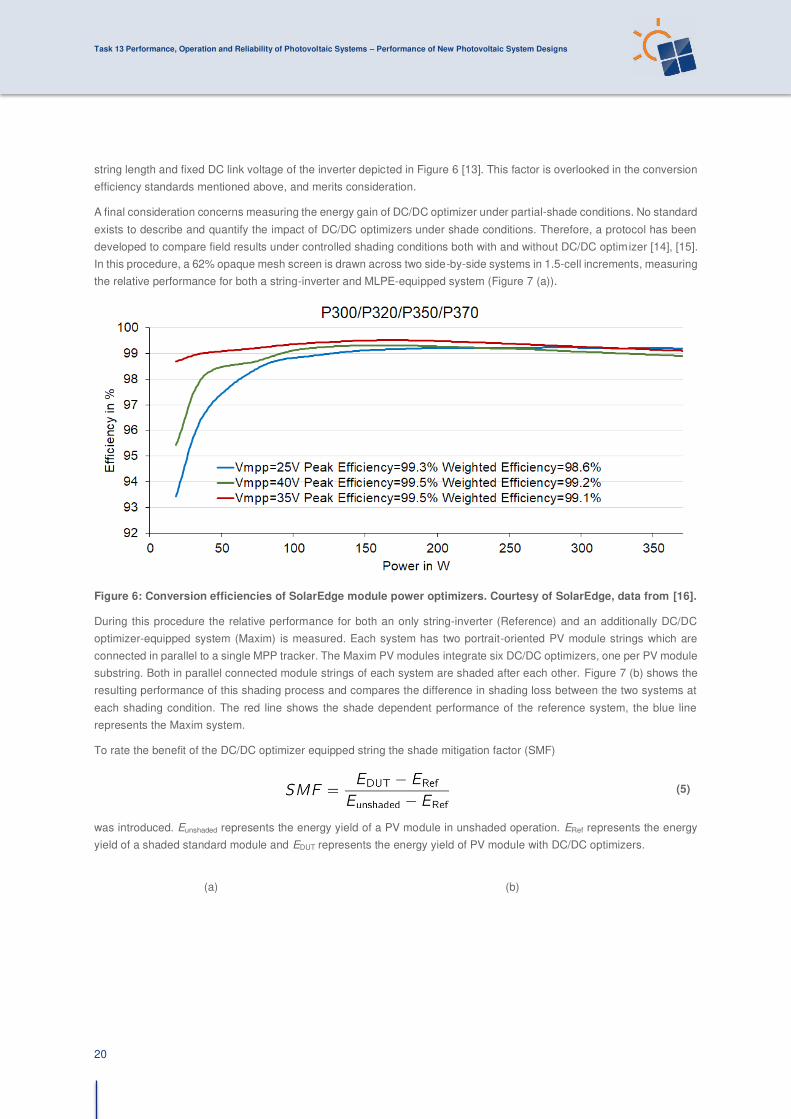
string length and fixed DC link voltage of the inverter depicted in Figure 6 [13]. This factor is overlooked in the conversion
efficiency standards mentioned above, and merits consideration.
A final consideration concerns measuring the energy gain of DC/DC optimizer under partial-shade conditions. No standard
exists to describe and quantify the impact of DC/DC optimizers under shade conditions. Therefore, a protocol has been
developed to compare field results under controlled shading conditions both with and without DC/DC optimizer [14], [15].
In this procedure, a 62% opaque mesh screen is drawn across two side-by-side systems in 1.5-cell increments, measuring
the relative performance for both a string-inverter and MLPE-equipped system (Figure 7 (a)).
Figure 6: Conversion efficiencies of SolarEdge module power optimizers. Courtesy of SolarEdge, data from [16].
During this procedure the relative performance for both an only string-inverter (Reference) and an additionally DC/DC
optimizer-equipped system (Maxim) is measured. Each system has two portrait-oriented PV module strings which are
connected in parallel to a single MPP tracker. The Maxim PV modules integrate six DC/DC optimizers, one per PV module
substring. Both in parallel connected module strings of each system are shaded after each other. Figure 7 (b) shows the
resulting performance of this shading process and compares the difference in shading loss between the two systems at
each shading condition. The red line shows the shade dependent performance of the reference system, the blue line
represents the Maxim system.
To rate the benefit of the DC/DC optimizer equipped string the shade mitigation factor (SMF)
(5)
was introduced. Eunshaded represents the energy yield of a PV module in unshaded operation. ERef represents the energy
yield of a shaded standard module and EDUT represents the energy yield of PV module with DC/DC optimizers.
(a) (b)

Task 13 Performance, Operation and Reliability of Photovoltaic Systems – Performance of New Photovoltaic System Designs
21
Figure 7: (a) Two side-by-side systems, one connected to a conventional string inverter and one with DC/DC
optimizer installed. Shading with 62% opaque fabric. In the foreground one of two PV module strings equipped
with DC/DC optimizers and shaded is shown. (b) Difference in performance loss for the two system configurations
with and without substring wise DC/DC optimizer under two portrait-oriented PV module strings subsequent
shaded in 1.5 cell increments [14].
A final composite shade mitigation score is calculated via the frequencies of each shade configuration. Typical Shade
Mitigation Factors of 30% - 40% are calculated, indicating that for typical residential shading, roughly ⅓ of the shading loss can be recovered by the investigated DC/DC smart modules [17], [14].
A measurement protocol for characterizing the performance of DC/DC optimizers under shading conditions has been
developed. Also, the Shade Mitigation Factor (SMF) was introduced to quantify the impact DC/DC operation under shading
conditions. Input data measurement data from specific use cases or simulation data from specific use cases. There are
no standardization processes regarding this topic, yet.
3.1.3 New performance characterization methods for AC modules
The use of microinverters provides flexibility of installation and safety due to lower system voltages to PV installers and
owners, particularly in small residential systems. When used as distinct components in a system, the PV module and
microinverter may be characterized individually with methods such as IEC 61853 [18] and EN 50530 [1].
An AC Module fully integrates the PV module with a microinverter such that there are no external DC connections. This
integration of PV module directly with microinverter eliminates or hinders the ability to characterize each component
separately. Instead, the fully-integrated AC Module must be characterized as a whole. In 2015, Sandia National
Laboratories developed a method for testing, characterizing, and modelling AC Modules [19].
At any given time, the AC module operates in one of three distinct states; the low-irradiance state, the self-limiting state,
or the typical operation state.
The AC module operates in a low-irradiance state whenever there is insufficient irradiance to power the inversion
electronics and the module may consume a small amount of active power from the electrical grid. The power in this state,
P3, is determined as
(6)
Here, PNT is the consumed active AC power in watts, and the power P3 is always negative to indicate that the AC module
consumes power in this low irradiance state. PNT may be obtained by specification sheets or determined empirically by
measuring power consumption when the module is not illuminated.

Task 13 Performance, Operation and Reliability of Photovoltaic Systems – Performance of New Photovoltaic System Designs
22
The microinverters within PV modules generally have some output power level at which they begin to limit their output;
this state is commonly known as “clipping”. In this self-limiting state, the output AC power remains constant despite
changes in irradiance which allow the PV panel to produce more DC power. The power produced in this state is determined
as
(7)
The value of PAC,max may be reported on a specification sheet or, preferably, determined empirically.
While the self-limiting power of the AC module is presented as a constant, if the modeler determines that the self -limiting
power of the AC module is a function of other input variables, the self-limiting power equation may be replaced with a more
accurate model.
While operating in the typical operation state the active power of the AC module changes as a function of irradiance, PV
cell temperature, and solar spectrum. While operating in this state, the active AC power is represented as the product of
a reference power and a series of normalized scaling factors.
(8)
where:
• PACref is the AC power under reference conditions Eref, AMaref, and T0, in watts
• f1 is an empirical unitless function which modifies the PV AC module output power as a function of absolute
(pressure corrected) airmass relative to the reference absolute airmass
• C0 is a unitless empirical coefficient describing the linear relationship between the irradiance and the PV AC
module output power, typical values near 1
• C1 is a unitless empirical coefficient describing the logarithmic relationship between the irradiance on the PV
AC module output power
• EPOA is the broadband POA irradiance incident upon the module which reaches the active PV material, in
W/m2. EPOA is estimated from measured broadband GPOA irradiance by accounting for the module losses due to
specular reflection and/or acceptance of diffuse irradiation.
• Eref is the reference POA irradiance in W/m2
• 𝛾AC is the PV AC module’s power output dependency to change in cell temperature in units of 1/°C
• TC is the cell temperature of the PV AC module in °C
• T0 is the reference cell temperature of the PV AC module, usually 25°C
Thus, in the typical operation state, the power is modelled as a function of incident transmitted irradiance, cell temperature,
and absolute airmass. Each of these factors is based on an underlying sub-model which are described in more detail in
[19]. The use of normalized scaling factors to adjust a reference power allows for further development of the model to
include other inputs that are not considered in this work or to utilize different sub-models to obtain more accurate scaling
factors.
With the performance of the AC module defined in three distinct operating states, the model then simply determines the
state in which the module is operating and uses the power model for that state.
(9)

Task 13 Performance, Operation and Reliability of Photovoltaic Systems – Performance of New Photovoltaic System Designs
23
To determine the reference conditions, reference performance, and sub-model performance parameters, Sandia
measured the module’s active power production in outdoor conditions over a period of several weeks with the AC module mounted on a 2-axis solar tracker. A series of tests, designed to isolate the performance parameters of each specific sub-
model, are performed on each AC module. While testing is explained in [19], we present a summary of the tests here.
• Thermal test to determine module temperature coefficients. The module power is measured as it is cooled to
ambient temperature and then allowed to heat via solar irradiance while remaining normal to the sun.
• Self-consumption test to determine the amount of active power consumed by the module in low irradiance
conditions. The module power is measured during low irradiance conditions.
• Angle-of-incidence test to determine the effect of solar incident angle on module power production. The
module power and solar incident angle are measured while the module is rotated away from the sun.
• Electrical performance test to determine the effect of changing solar irradiance, solar spectrum, wind speed,
and ambient air temperature. The module is tracked normal to the sun for several days to weeks as its power
is measured. A range of different weather conditions are desired.
This testing allowed for the AC module to be measured under a wide range of incident irradiance, spectra, and temperature
to derive model parameters that predict AC module active power to within ±2% which Figure 8 and Figure 9 confirm.
Figure 10 shows the measured and modelled power from an AC PV module on a cold, breezy, partly clouded day. Prior
to sunrise, the module operates in the low-power state, where the AC module consumes approximately 0.6 watts of active
power. As the sun rises and illuminates the AC module, it begins producing active AC power according to the incident
irradiance and module temperature. In the middle of the day, the AC module is limiting its output power, producing a
constant amount of power, regardless of increasing incident irradiance.
Figure 8: PV AC module model residuals on data used within the parameter estimation data set [19].

Task 13 Performance, Operation and Reliability of Photovoltaic Systems – Performance of New Photovoltaic System Designs
24
Figure 9: Histogram of model power residuals over 9 days for a fixed-tilt PV AC module, daytime data only [19].
While Sandia National Laboratories conducted performance testing outdoors, indoor performance testing of AC modules
may be possible. However, due to the lag and self-consumption of power within the attached microinverter, a continuous
light source would be required and some performance characteristics could need to be estimated if they could not be
measured directly via indoor testing.
The testing and analysis produce a performance model for each AC PV module. The models developed by Sandia were
tested and validated over 9 days, during which the AC module was held at a fixed tilt while its power was measured. During
the validation period, the model produced a (daytime) root mean square error (RMSE) less than 1% and predicted the
total power generation within 1.4%.
The described measurement protocol and simulation model for PV AC modules enables to conduct simulations for specif ic
use cases. With the generated results like time series of the PV AC module´s AC power or the energy yield performance
indicators for the specific use case can be calculated.

Task 13 Performance, Operation and Reliability of Photovoltaic Systems – Performance of New Photovoltaic System Designs
25
Figure 10: Measured and modelled power from a fixed-tilt PV AC module on a cold, breezy, partly cloudy day [19].
3.1.4 Module-level Power electronics under indoor performance tests
Due to the electrical wiring of conventional PV systems with string inverters and their centralized maximum power point
tracking (MPPT), partial-shading conditions have a great impact on the reduced performance of those systems. Module-
level power electronics (MLPE) e.g. microinverters or power optimizers (DC/DC-converter) apply individual MPPT for each
PV module. Thus, the annual system performance will increase, if the total MLPE efficiency for the unshaded events is
not significantly lower compared to sting inverter. Claims of two-digit number percentage of performance gain of MLPE
relative to standard string inverters could not be verified by intensive indoor lab test at ZHAW for typical roof shading
conditions.
Figure 11 shows the simulated system with the PV module placement on the roof and a dormer, throwing a shadow on
two PV modules in the late morning for instance. The roof inclination is 30° with a south facing module plane.
Figure 11: Simulated system with the PV module placement on the roof with a dormer [20].
The origin of the corresponding daily course of DC output of ten rooftop PV modules facing typical shading conditions of
a dormer are a measurement run of a real system. Detailed ray tracing shading models calculate the time series of the
DC current and voltage output of one individual PV module, with a spatial resolution of a single solar cell within the standard
PV module of 60 cells and three bypass diodes.
Figure 12 show the I-V curves of one module and the graphical representations of three different shading situations with
a 1%, 47% and 50% shading of one cell (marked in red).

Task 13 Performance, Operation and Reliability of Photovoltaic Systems – Performance of New Photovoltaic System Designs
26
(a)
(b)
(c)
Figure 12: I-V curve of one module and graphical representation of three different shading situations with (a) 1%,
(b) 47% and (c) 50% shading of one cell at 1:26 pm, 1:38 pm and 1:41 pm.
The indoor test setup uses ten serials connected commercial MLPE devices feeding the commercial DC/AC inverter. An
overview of the used laboratory hardware setup is visualized in Figure 13. Ten solar array simulators (SAS) individually
controlled powering each MLPE device. To assess the performance of the power optimizer system over one day, the SAS
devices received the values for IMPP, ISC and UMPP, UOC every 5 seconds, based on precalculated I-V curve values of a PV
module from the system simulation. The testing was performed over 12.5 hours.

Task 13 Performance, Operation and Reliability of Photovoltaic Systems – Performance of New Photovoltaic System Designs
27
Figure 13: Electrical lab setup to measure the performance of the MLPE system with ten power optimizers. [20]
In Figure 14 (a), the power before and after the DC/DC conversion of the real-time irradiation test for four power optimizer
is visualized, due to limited power range of the SAS devices, the curve was flattened between hour 10 and 14. Still, the
effects of shading are most prominent between hour 7 and 10. Additionally, the resulting efficiency of the power optimizer
is shown, whereby a plunge in efficiency in shaded conditions of approximately 5% to a value of 90% in average can be
discerned.
In order to determine a performance rating of the system during realistic operating conditions, a weighted efficiency value
ηavg,wgt was calculated at each timestep t during the real-time test according to equation (10). Pout,Opt is the output power of
the DC/DC optimizer Opt, N represents the total number of DC/DC optimizers in the system, Pout,mean,N indicates the mean
output power of all N DC/DC optimizers and ηOpt is the efficiency of the DC/DC optimizer Opt.
(10)
The resulting ηavg,wgt for the assessed system is 96.79% as visualized by the dashed red line in Figure 14 (b). The efficiency
can be expected to be slightly higher in the case with modules with a lower UMPP (i.e. lower voltage ratio).
(a) (b)

Task 13 Performance, Operation and Reliability of Photovoltaic Systems – Performance of New Photovoltaic System Designs
28
Figure 14: (a) Plot of the real-time irradiance testing with input and output power of four MLPE power optimizers
and respective efficiency values in function of time. (b) Plot of the real-time irradiance test with input and output
power of four MLPE power optimizers and respective voltage ratio values in function of time.
The measured efficiency of an individual DC/DC MLPE without the final DC/AC inverter over the input Power Pin is given
in Figure 15. Figure 16 shows the measured efficiency of an individual DC/DC MLPE without the final DC/AC inverter over
the voltage ratio UDC,in/UDC,out.
Figure 15: Electrical setup of the analysed MLPE system with 10 optimizer and respective DC/DC efficiencies for
a power range from zero to 140 Watts. Accordingly fitted function shows the approximate course of DC/DC
efficiencies for the DUT Solaredge P405 in the shown power range.
Efficiency values below 98% and for most of the real conditions below 97.5% are revealed. This is 1% below the given
values in the manufactures datasheet and could by more than 2% lower than that, if the planer is not aware of the relevance
of the ratio of the input and output voltage of the optimizers. Efficiency values of 97.5% and up to 98% could be reached
if the ratio of DC input relative to DC output voltage is between 0.8 and 1.4. The nearly linear further decay of the efficiency
will be below 93% at a ratio of 3.5. Latter is below the average efficiency of old inverters common two decades ago. It is
recommended that the MLPE manufactures should give this efficiency characteristics in their datasheets, like it was done
in the early days of PV inverters to show the DC voltage dependency on the DC/AC and the weighted EURO, CEC
efficiency [21],[22]. Today, PV string inverters see an 98.5% (CEC rating), up to 99% max rating and this highly relevant
to compare the unshaded performance of MLPE and string systems. For the detailed analysis of the MLPE system
efficiency, the fixed mode of the SAS was used to set static values in an interval of 5 seconds. In detail, a voltage ran ge
of 12 to 78 V with 2 V steps and a current range of 0.2 to 5 A with 0.1 A steps was tested and evaluated.
91%
92%
93%
94%
95%
96%
97%
98%
0 10 20 30 40 50 60 70 80 90 100 110 120 130 140
η DC
/DC
Pin [W]
Opt. 1 Opt. 2Opt. 3 Opt. 4Opt. 5 Opt. 6Opt. 7 Opt. 8Opt. 9 Opt. 10FIT

Task 13 Performance, Operation and Reliability of Photovoltaic Systems – Performance of New Photovoltaic System Designs
29
Figure 16: Measured efficiency of one individual MLPE DC/DC converter as a function of the ratio of input and
output DC voltage. The input power and input voltage are indicated during different selected shading condition
during the day.
The average efficiency value for each 1-Watt bin is visualized in Figure 17 and the maximum efficiency is found at 171 W
with a value of 97.21%. The difference to the datasheet value of 2.29% is significant. However, due to the strong
dependency of the efficiency of the DC/DC conversion on the input to output voltage ratio, the average values are not a
general reference for every operating condition. It also depends on the absolute DC voltage level, with higher efficiency
values at higher voltage (see Figure 16). Therefore, curve fitting for the measurement values for three different voltage
ratios, namely, 0.6, 1.15 and 2.3, ± 0.1, were determined. As expected, the average efficiency values for a power of more
than 180 W are influenced by the suboptimal voltage ratios of > 1.75. In addition, an approximated EURO and CEC
efficiency was calculated, which uses the values at 90% of nominal power instead of at 100%, due to the limited power
range of the SAS devices. Both values resulted in 96.61%, which is visualized in Figure 17 and indicated by the horizontal
dash-dotted line. Finally, highest efficiency values of 98% was measured in a narrow field at voltage ratios of 0.99 to 1.1.
Due to the reason that the efficiency of the power optimizer varies greatly with the ratio of voltages, they were determined
and visualized in Figure 17. Furthermore, the average voltage ratio is visualized with a value of 2.054 and the power
weighted voltage ratio with a value of 1.586.

Task 13 Performance, Operation and Reliability of Photovoltaic Systems – Performance of New Photovoltaic System Designs
30
Figure 17: Efficiency values of the DC/DC conversion of the power optimizers as a function of the input power
and voltage ratio (in/out) based colouring with colour bar.
The resulting efficiencies are only representative for a lower range of irradiance conditions. First approximations of the
devices’ performance were achieved and are shown in Table 2.
Table 2: Resulting efficiency values of the devices.
Name Device Measured Absolute difference to datasheet
ηDC/AC SE3500 97.40% -0.20%
ηDC/DC,max avg P405 97.21% -2.29%
ηDC/DC,power wgt P405 96.79% -2.71%
ηDC/DC EURO & CEC P405 96.61% -2.89%
Finally, the resulting efficiencies of the power optimizer and the PV-inverter were multiplied, and therefore, the total system
performance estimated, which are stated in Table 3.
Table 3: Total performance of the MLPE system.
Name Resulting total system η
ηTotal max avg 94.78 %
ηTotal power wgt 94.37 %
ηTotal EURO & CEC 94.19 %

Task 13 Performance, Operation and Reliability of Photovoltaic Systems – Performance of New Photovoltaic System Designs
31
Due to the limited power range of the SAS devices, an increased voltage and lower current was used during the testing.
This has the potential to reduce the efficiency values of the power optimizers. Still, the total system performance value
(e.g. the total power weighted efficiency) shows a significant deviation of approximately -2.27% from the potential
efficiency, estimated by the combined MLPE system datasheet values.
If there is a specific shading situation, the benefit of MLPE, must be determined on a case-by-case basis. There is not a
general statement available for all cases. As for the simulated PV system, an additional daily yield of approximately 3.5%
was calculated for the use of MLPE. The results of the simulation are stated in Table 4.
Table 4: Simulation result of a clear-sky day with the sun path of the 20th March at Winterthur, Switzerland, and
updated efficiency values for the system with MLPE.
System type ηTotal power wgt Simulated daily yield
MLPE 94.37% 103.50%
String inverter 97.00% 100.00%
In scenarios with extreme and inhomogeneous shading a MLPE system provides a significant advantage. Whereas for
low shading situations, these systems are generally expected to yield less energy than conventional systems. On the other
hand, the course of the shade on the module is of key importance. As for example, a shade, which is orthogonal to the
cell strings (as in the simulation), will lead to significant losses in a conventional system. Accordingly, various shading
situations must be examined with the indoor test facility presented in this paper and also applied by other independent
laboratories.
3.1.5 Performance of new shade resilient module designs
Analysis of PV energy yields of PV systems reveals in many cases that the actual yield may be lower than the expected
yield. The latter is based on an appropriate description of system parameters and actual irradiance and other
meteorological parameters such as ambient temperature and wind speed. A MPPT is used to optimize power generation
by the PV system. Besides system or components’ failures, shading is a prominent cause of performance loss, especially in the built environment, which may amount to perhaps 10% loss on an annual basis [23]. As multiple PV modules are
usually connected in series to central inverters, shading-induced power losses at the module level will negatively influence
the maximum attainable system power. Also, partially shaded modules and in particular cells in these modules may
become reverse biased and will act as a load consuming power generated by the other, unshaded, cells. This may lead
to increased cell temperatures, or hot spots [24], which may lead to faster degradation of both diode and PV module in
case of partial shading. The use of bypass diodes will limit this, by bypassing shaded substrings of the solar module.
Typically, three bypass diodes are used in antiparallel connection to the cells per 60/72-cell module [25], leading to power
loss of 1/3, or 2/3 upon partial shading. However, adding more bypass diodes thus increasing granularity of cell groups
can increase performance, especially under partial shading conditions [26]–[28].
It is obvious that optimum design in terms of string connections and use of central inverters should take potential shading
effects into account. Another approach would be to apply module level power electronic which aims to optimize the
maximum power of individual PV modules [29]. This has been available commercially for some years now, and system
designers are challenged to find an optimum between additional cost and additional yield, which will depend on the
expected shading loss.
Mitigation of shading effects on PV performance can be classified in two groups [30]: circuit-based topologies, and modified
MPPT based techniques. These are usually applied on a per-module level. For example, increasing the number of bypass
diodes, or so-called total cross tied topologies, which can be fixed connections between cells in a module or adaptive
connections. The latter topology requires microcontrollers that control a switching matrix, and indeed mitigate shading, but
is quite complex by design, and not so fast [31]–[33]. In the following, two examples of shade mitigation strategies are
described.

Task 13 Performance, Operation and Reliability of Photovoltaic Systems – Performance of New Photovoltaic System Designs
32
Increasing module granularity
This section gives at first a short overview of PV module topologies with different module integrated electronics.
Subsequently simulation results are discussed, rating the different PV module topologies´ potential of shade mitigation.
One alternative strategy for mitigation of nonlinear shading effects is to divide the cells in the module into smaller groups
of cells and apply an active bypass diode for each group of cells, instead of using a passive bypass diode [34]. An active
bypass diode actually is an electrical circuit consisting of Metal-Oxide-Semiconductor Field-Effect Transistors (MOSFETs),
which can be controlled via a duty cycle as control signal. Such module integrated electronics (MIEs) can be categorized
in the following groups [34]: (i) conventional systems, consisting of three bypass diodes per module and a central converter
to change the output voltage level; (ii) buck converters, to which normal PV modules are connected and thus the output
current of the shaded module is to be controlled; (iii) buck-boost converters, in which both current and voltage are to be
controlled; and (iv) voltage equalizers, which are a combination of different converters or even bidirectional converters to
equalize the voltage by power processing [35]–[37].
In conventional modules, the cells are generally grouped in three groups of series connected cells and to each group one
bypass diode is connected in parallel. The MPPT algorithm of the (string) inverter optimizes the generated power. MIEs
using buck or buck-boost converters are potentially interesting for controlling current or voltage and current of the shaded
cell group [34].
(a)
(b)
Figure 18: (a) Smart module architecture with ng cells in NG groups with electronic circuits, (b) contour plots of
efficiency as a function of input and output current for a smart module with ten groups of six cells [34].
While in the ultimate case with ideal lossless bypass diodes one bypass diode per cell shade mitigation is optimal, this is
certainly not economically and technically optimal due to losses of real bypass diodes. Hence, a compromise must be
sought between the number of bypass diodes, and thus groups of series-connected cells NG. Figure 18 (a) shows the
principle design of a module with ng solar cells in NG groups of cells in a module [34]. Using 60 monocrystalline silicon
solar cells (open circuit voltage (VOC) of 613 mV, short circuit current (ISC) of 7.92 A, maximum power (Pmax) of 3.7 W,
efficiency η of 15.4%) and a number of DC/DC converters, in this case Linear Technology LTM4611, the optimum
configuration in terms of converter efficiency has been determined. Figure 18 (b) shows the efficiency contour plots, for a
module with ten groups of six cells. Specifications per group are thus: VOC = 3.67 V, ISC = 7.92 A, Pmax of 22.18 W. Because
of the system topology, the output current flow of each converter is equal as all converters are connected in series. This
strategy extracts as much power as each group of cells could generate, even though some groups may be very heavily
shaded. In the smart module architecture all cells, even shaded ones, are thus producing power efficiently and none of
the cells is bypassed.
Four different module topologies have been modelled and simulated to assess the shading mitigation potential: (1) an so
called ideal module, in which for each cell a DC/DC converter is responsible to level up the current for shaded cells, (2)
smart module with ten groups of six cells in which for each group a DC/DC converter is operated, (3) a module with three

Task 13 Performance, Operation and Reliability of Photovoltaic Systems – Performance of New Photovoltaic System Designs
33
parallel to a DC/DC converter connected strings with each string consisting of 20 cells connected in series and a blocking
diode (normally this topology is implemented for strings of PV modules instead of PV cells) and (4) a standard module
with series-connected strings, operated with a DC/DC converter, consists of three series groups of 20 cells, where each
group is equipped with one bypass diode.
(a)
(b)
(c)
Figure 19: Effect of different shading patterns on different module topologies, (a) combined pole and random
shading pattern, (b) pole shading pattern, (c) no shade [34].
Figure 19 shows the simulated output power for three different shading patterns on different module topologies. The power
of the ideal module clearly reflects the shade that is cast on the module. This is most clear in Figure 19 (a). Current and
voltage of the series/parallel module is considerably affected by the shade Figure 19 (b), in which only the edge of the
module is shaded reveals that two groups of cells in the smart module are affected, and 1/3 of the series/parallel module.
Module power is nearly equal when there is no shade as shown in Figure 19 (c), illustrating some loss in the smart module,
see also Table 5. Table 5 compares the output power of the different introduced four module architectures under the three
shading patterns show in Figure 19 (a)-(c).
Task 13 Performance, Operation and Reliability of Photovoltaic Systems – Performance of New Photovoltaic System Designs
34
Table 5: Output power for three different shading patterns, as shown in Figure 19 [34].
Architecture a) combined pole and random shading pattern [W]
b) pole shading [W]
c) no shade [W]
Ideal 48.35 84.23 116.54
Smart 18.49 69.00 108.85
Series connected 0.84 30.95 112.35
Parallel connected 4.51 62.97 113.42
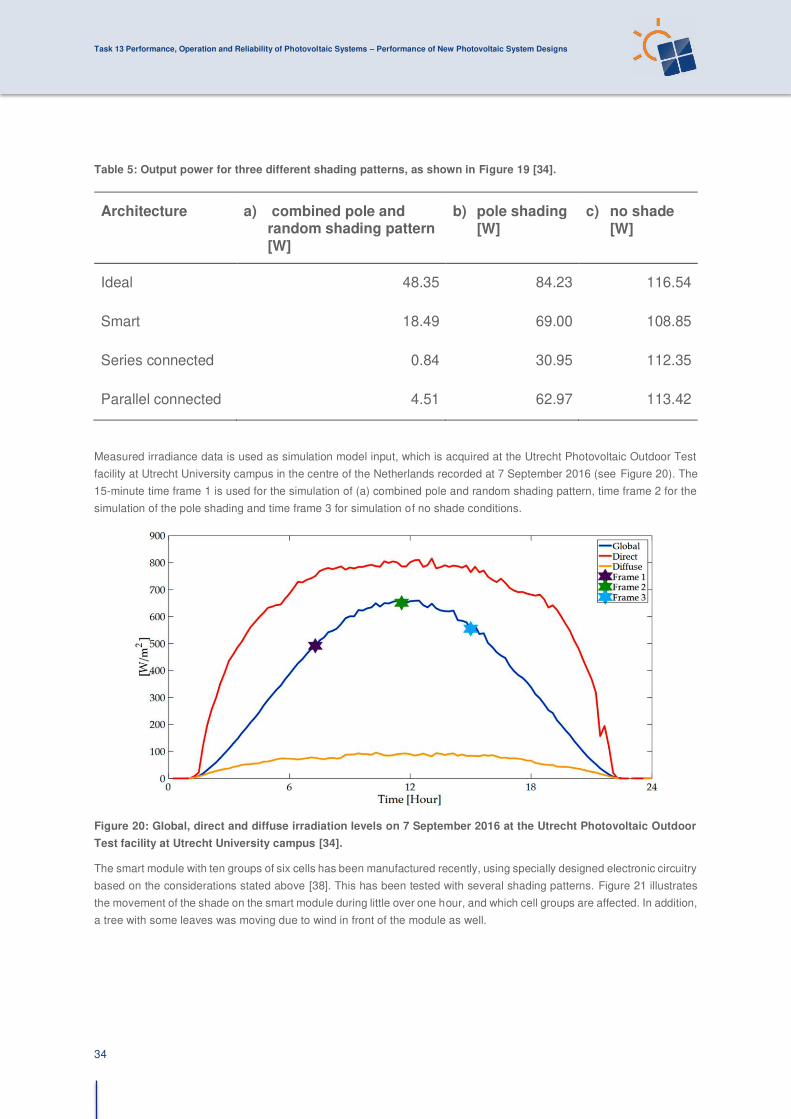
Measured irradiance data is used as simulation model input, which is acquired at the Utrecht Photovoltaic Outdoor Test
facility at Utrecht University campus in the centre of the Netherlands recorded at 7 September 2016 (see Figure 20). The
15-minute time frame 1 is used for the simulation of (a) combined pole and random shading pattern, time frame 2 for the
simulation of the pole shading and time frame 3 for simulation of no shade conditions.
Figure 20: Global, direct and diffuse irradiation levels on 7 September 2016 at the Utrecht Photovoltaic Outdoor
Test facility at Utrecht University campus [34].
The smart module with ten groups of six cells has been manufactured recently, using specially designed electronic circuitry
based on the considerations stated above [38]. This has been tested with several shading patterns. Figure 21 illustrates
the movement of the shade on the smart module during little over one hour, and which cell groups are affected. In addition,
a tree with some leaves was moving due to wind in front of the module as well.
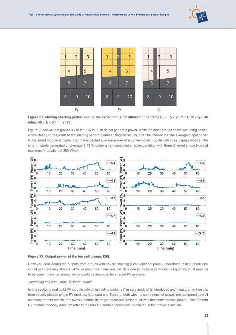
Task 13 Performance, Operation and Reliability of Photovoltaic Systems – Performance of New Photovoltaic System Designs
35
Figure 21: Moving shading pattern during the experiments for different time frames (0 < t1 < 20 mins; 20 < t2 < 40
mins; 40 < t3 < 60 mins [38].
Figure 22 shows that groups six to ten (G6 to G10) do not generate power, while the other groups show fluctuating power,
which clearly corresponds to the shading pattern. Summarizing the results, it can be inferred that the average output power
in the smart module is higher than the expected average power of a conventional module with three bypass diodes. The
smart module generated on average 8.13 W under a very restricted shading condition with three different shade types at
maximum irradiation of 350 W/m2.
Figure 22: Output power of the ten cell groups [38].
However, considering the outputs from groups with severe shading a conventional panel under these testing conditions
would generate only about 1.64 W, or about five times less, which is due to the bypass diodes being activated. It remains
to be seen in how far annual yields would be improved for shaded PV systems.
Increasing cell granularity, Tessera module
In this section a real build PV module with a high cell granularity (Tessera module) is introduced and measurement results
from equally shaded single PV modules (standard and Tessera, both with the same nominal power) are compared as well
as measurement results from two six-module fields (standard and Tessera, all with the same nominal power). The Tessera
PV module topology does not refer to the four PV module topologies introduced in the previous section.

Task 13 Performance, Operation and Reliability of Photovoltaic Systems – Performance of New Photovoltaic System Designs
36
The Tessera solar module concept [39], [40], named after ‘tesserae’ being used as individual tiles in ancient mosaics,
makes use of small cells that are cut by laser scribing from 156 x 156 mm2 silicon cells. The used cells are 6-inch metal
wrap through (MWT) c-Si cells, which have been cut to produce 16 mini cells. These are interconnected in series, and
connected to a bypass diode that is laminated in the back sheet. Being back contact solar cells, interconnection schemes
can be designed using a conductive backsheet, which thus allows to integrate diodes, see Figure 23 (a).
(a)
(b)
Figure 23: (a) Building block of Tessera module concept consisting of four full size MWT cells, (b) full module of
1.6 m2 consisting of 960 mini cells [24].
Blocks of 64 mini cells can then be connected in parallel forming modules with custom size and rated power (see Figure
23 (b)). This module building block shows VOC of around 40 V and ISC of 0.6 A, under standard test conditions [40]. A
standard module size of 1.6 m2 comprises 15 of these module building blocks of 64 mini cells that are connected in parallel,
thus yielding ISC of 8 A, and module rating of 265 Wp. Module manufacturing equipment is the same as for standard back
contact modules, albeit with a small modification in the production line.
The design of the blocks is optimized for shade resilience. The sub cells can be regarded as pixels, and only a shaded
pixel will be affected by the shade, and not 1/3 of a (standard) module. Because of a somewhat different output compared
to a standard module, a dedicated inverter may be required. However, the voltage of the module is almost independent of
shading conditions, which would make inverter design less complex [41].The performance of the Tessera module has
been experimentally tested and compared to a standard module. To this end, artificial shading conditions have been
applied while using a solar simulator. Note, the absence of diffuse irradiance exaggerates the results somewhat. The
shade performance was defined as the ratio of maximum power obtained in a shading condition and the maximum power
of a standard 3-string module. Another measure is the shade linearity. This will be 100% if a x% sized shade will lead to
the same x% of power loss induced by that shading [40]. As shading conditions, a pole, a dormer and a tree have been
used. Table 6 shows that the Tessera module considerably outperforms the standard module both for shade performance
as well as shade linearity.

Task 13 Performance, Operation and Reliability of Photovoltaic Systems – Performance of New Photovoltaic System Designs
37
Table 6: Effect of shading conditions on the shade performance and shade linearity of the Tessera module
compared to standard module [40].
Shadow type Shade performance Shade linearity
Standard module [%] Tessera [%] Standard module [%] Tessera [%]
Pole 17 67 20 76
Dormer 26 64 38 92
Tree 53 73 66 92
Obviously, the advantage of using a Tessera module rather than a standard module depends on the actual shape and
size of the shading condition. A PVsyst simulation has been performed for a house with a dormer in an urban environment
with trees and a lamppost, with PV modules on its roof. On an annual basis, the simulations show that a shade -induced
loss of 11% is incurred for the standard module, while the Tessera module shows only 7% loss. Thus, the Tessera module
shows a 4% higher energy yield compared to a standard module. This average advantage may seem low, but the
simulation includes hours in the year for which no shade is cast on the modules. The yield advantage can be much higher
in winter months, where shading is adversely affected PV yield (see also [23]). For example, a sunny hour in January
shows a yield advantage of 24% [40].
Figure 24: Normalized power output of a Tessera and standard module under the same partial shading conditions
[42].
A field test with six 265 Wp Tessera modules has been performed comparing their performance to two reference systems,
all with the same orientation and tilt: one with six standard modules, also of 265 Wp capacity each, connected in series to
a string inverter (SI), and one with six standard modules each equipped with a microinverter (MI) [42]. The Tessera
modules are also connected to individual microinverters. A pole shade has been used for assessment of part ial shading
effects.
Figure 24 compares the normalized power outputs of the Tessera and reference module under identical shading conditions
of a day in winter. The pole affects the performance of the modules between 1 pm and 4:30 pm, while in the morning
power generation is identical. For this particular day, the Tessera module generates 15% more energy than the reference
module. Interestingly, micro inverter efficiency is somewhat higher in case of the Tessera module due to the more stable
voltage output of the module. The shade leads to voltage reduction of about 1/3 for the reference module.

Task 13 Performance, Operation and Reliability of Photovoltaic Systems – Performance of New Photovoltaic System Designs
38
This can also be seen in Figure 25, where DC voltage, relative power output and micro inverter efficiency for a period of
six months is shown. Besides the cloud of points between ~27 V and ~37 V, for both modules, another cloud of points is
visible around 20 V. All in all, inverter efficiency is 2-3% higher in case of the Tessera module [42].
(a)
(b)
Figure 25: Relation of voltage, power and efficiency of the micro inverters for the reference ((a) and Tessera ((b)
system [42].
A further comparison of measured data is shown in Table 7. This shows that in this test with the pole shade present in the
afternoon (see Figure 24) micro inverters yield higher AC performance ratio than the string inverter. The higher MI
efficiency for the Tessera module due to more stable voltage levels is also corroborated here. Based on these results, it
is estimated that annual shading loss in residential systems with Tessera modules and microinverters would be similar to
a module with one bypass diode per cell. Compared to standard modules with three bypass diodes, annual shading loss
would be decreased from 9.3% to 3.3% [24].
Table 7: AC performance ratio for the three modules systems [28].
Module/inverter system Months
Feb Mar Apr May Jun Jul Aug Sep
Tessera/MI 0.91 0.88 0.85 0.84 0.83 0.81 0.76 0.84
Standard/MI 0.88 0.87 0.83 0.80 0.85 0.81 0.73 0.82
Standard/SI 0.76 0.84 0.81 0.77 0.84 0.78 0.68 0.78
The measurement protocol presented here is suitable to show advantages of the Tessera PV module configuration in
specific shaded operation compared to standard PV modules. In order to provide information about the effect of shade
resilient PV modules on the energy yield, or other performance indicators for specific PV systems operating under dynamic
shading conditions in the course of a year a measurement protocol respecting dynamic shading has to be developed.

Task 13 Performance, Operation and Reliability of Photovoltaic Systems – Performance of New Photovoltaic System Designs
39
4 PERFORMANCE CHARACTERIZATION OF COMPLEX NEW SYSTEMS WITH PV
4.1 Transient PV battery quotation according to the NESPRESSOTM1-test
PV Battery systems show different transient behaviour. System parameters are derived from the measured step response
characteristics like dead-time, settling-time as it is commonly used in the technical field. This is in accordance with the
German Energy Storage Association (BVES) and German Solar Industry Association (BSW) efficiency guidelines [43]
described in section Erreur ! Source du renvoi introuvable..
The end customers of a PV battery storage system in a single-family house require decision-making facts during the
purchase phase that they understand. Thus, the Zurich University of Applied Science (ZHAW) Institute of Energy Systems
and Fluid Engineering (IEFE) proposes a very practical transient figure to describe the speediness of that storage system
to provide a standard coffee machine with stored solar power.
Figure 26: Test setup to measure the amount of Energy coming from the battery to supply a NespressoTM1 coffee
machine at ZHAW IEFE [44].
During the NESPRESSOTM1-test the quotation of used electricity coming from the battery compared to grid electricity is
measured. A standard small single cup NespressoTM1 machine is used as consumer load which was connected to the test
setup given in Figure 26.
To rate the speed of the battery storage control system a NespressoTM1-ratio with
1 The trademarks, trade names, logos, service marks, domain names or other distinctive brand features of Nespresso (“Trademarks”) displayed are the exclusive property of Nespresso and/or Nestlé.

Task 13 Performance, Operation and Reliability of Photovoltaic Systems – Performance of New Photovoltaic System Designs
40
(11)
was introduced. It is the ratio of EBat the energy the battery storage system supplied during the coffee making process and
the energy ENespressoTM1 totally used for coffee making by the coffee machine.
Figure 27 shows during the 90 s it takes to brew one cup of coffee the used electrical power cycles between 1200 W and
0 W in red and the power delivered from the battery system in yellow. In this example the delivered power from the battery
system lag vast behind the consumer need. So finally, the performance indicator Nespresso TM1-ratio is only 1/8. One part
of the used energy comes from the battery out of 8 energy units – illustrated by green and red Nespresso cup symbols.
Figure 27: Measurement results of the Nespresso Test of an AC coupled PV Battery System is given with the
customer load of the coffee machine - in red - and the power delivered from the battery system – yellow, with the
result of only 1/8 of the used energy coming from the battery [44].
This Nespresso TM1 use case shows how important meaningful key performance indicators for PV battery storage systems
regarding real operating conditions are. Indicators like the nominal battery capacity, or the maximum battery inverter
efficiency as often found in data sheets are not meaningful. Besides the Nespresso ratio in section Erreur ! Source du
renvoi introuvable. regarding BVES/BSW efficiency guidelines further key performance indicators and measurement
protocol for PV battery systems are described [43].
4.2 Using a dynamic system model to characterize a complex PV system
Characterizing a PV system component completely requires knowledge of each power flow path leading into and leaving
this component, as well as the respective efficiency curves. At the Institute for Solar Energy Research Hamelin ISFH, a

Task 13 Performance, Operation and Reliability of Photovoltaic Systems – Performance of New Photovoltaic System Designs
41
dynamic simulation model was developed for the evaluation of PV storage concepts. It calculates the electrical power
flows between the system components PV generator, battery, electrical household load (HHL) and distribution grid. Thus,
the losses occurring in the system can be localized for any load and irradiance conditions.
4.2.1 Simulation model
The simulation model only considers the active power flows of conversion paths shown in Table 8 in the PV storage system
to determine the efficiency:
Table 8: Conversion paths in PV storage systems.
Conversion paths Description of power flows
PV2AC PV power for direct load coverage and grid feed-in
PV2BAT PV power for battery charging (AC system: PV2BAT consists of PV2AC and AC2BAT)
BAT2AC Discharge power from the battery to cover the load
The described conversion paths are shown in Figure 28 for a DC- and AC-coupled PV storage system. The power-
dependent efficiencies of the conversion paths are determined by measurements at the points sketched in light blue.
(a)
(b)
Figure 28: Schemes depict the conversion paths in the DC-coupled (left) and AC-coupled PV storage systems
(right) including the measurement points required for system characterization (light blue) [45].
The amount of power flows between the system components depends primarily on the PV generator power, the e lectrical
load and the dimensioning of the storage. The variable input variables for the simulation model are the irradiation intensity
at PV module level, the module, and the ambient temperature, as well as the electrical load PLOAD. The power flows in the
system are calculated according to four steps.
In the 1st step the power for direct load coverage PPV2LOAD is calculated. The possible invertible ( ’ for invertible) PV output PPV,AC’ results from the output of the PV generator PPV,DC and the conversion efficiency of the inverter ηPV2AC.
(12)
PPV2LOAD corresponds to the smaller value of the total invertible PV power and the power value of the load profile, limited
by the nominal power of the PV inverter:
. (13)
The charging power PPV2Bat or discharging power PBAT2AC at the battery terminals in self-consumption-optimized operation
is calculated in the 2nd step. Two cases must be distinguished here:

Task 13 Performance, Operation and Reliability of Photovoltaic Systems – Performance of New Photovoltaic System Designs
42
(a) Calculating the charging power of the storage PPV2Bat for PPV,AC’ > PLOAD, DC- and AC-coupled systems have to be
distinguished. To determine the charging power PPV2Bat, the excess PV power PBat,AC’ (AC-side) and PBat,PV’ (DC-side) are
first determined by
, (14)
. (15)
The auxiliary variable PLOAD,DC describes the DC PV power required to cover the load
.
(16)
The excess PV power consumed by the battery is limited by the system-specific, charge condition-dependent maximum
charge power (PBat,AC’ limited by PBat,AC and PBat,PV’ limited by PBat,PV):
AC-coupling: , (17)
DC-coupling: . (18)
(b) For both system topologies the DC discharge power PBAT2AC for PPV,AC’ < PLOAD is:
.
(19)
In the 3rd step the exchange power with the grid PGrid is calculated. If the battery is unable to compensate the residual
load from PV feed-in and household load PLoad the remaining power is fed into the grid (PGrid positive) or drawn from it
(PGrid negative)
. (20)
In the DC-coupled system, while the battery is being charged, PGrid is modelled as
(21)
PVB describes the power consumption of the PV inverter, battery converter and power meter at the grid connection point
(GCP) for the various operating modes "idle", "standby" and "sleep".
As a 4th step the state of charge C of the battery (in kWh) is calculated. It influences the maximum charging and
discharging power in the next time step.
(22)
The power PSPV describes the battery losses, determined from several charging cycles as a function of the charging power.
E. g. Typical self-discharge rates are 20% per month for lead-acid storage and 2% per month for Li-ion [46].
For the evaluation of the PV storage systems the share of self-consumption and the degree of self-sufficiency are
calculated as:

Task 13 Performance, Operation and Reliability of Photovoltaic Systems – Performance of New Photovoltaic System Designs
43
(23)
(24)
The system efficiency ηSys describes the PV energy used to cover the load and fed into the grid in relation to the amount
of energy fed into the system.
(25)
4.2.2 Parameterization of the simulation model
The above introduced simulation model is parameterized with the usable storage capacity, the performance-related
storage losses and the efficiency characteristics of the paths PV2AC, PV2BAT and BAT2AC measured in a laboratory [47]
or taken from data sheets. The efficiency of the PV2BAT conversion path for an AC-coupled PV storage results from the
partial conversions PV2AC and AC2BAT (ηPV2BAT=ηPV2AC*ηAC2BAT). Additionally, the transfer functions of the entire PV
storage systems must be considered. They strongly depend on the inertia and deviation of the MPP tracking of the PV
inverter and of the Battery Management System. Based on laboratory measurements they are adjusted individually. Static
control deviations were not considered in the model.
4.2.3 Validation of the simulation model
The model was tested on the basis of two systems in one-day comparison measurements. As a validation example, Figure
29 shows the modelled and measured power flows of an AC-coupled lithium-ion battery matching very well.

Task 13 Performance, Operation and Reliability of Photovoltaic Systems – Performance of New Photovoltaic System Designs
44
Figure 29: Comparison of the simulated performance at the battery terminals and at the GCP with a one-day
laboratory measurement (AC-coupled lithium-ion battery) [45].
Table 9 shows the system parameters determined for simulation and measurement. The characteristic values for the DC
system match even better.
Table 9: Comparison of the calculated and measured assessment parameters.
DC-System (Lead-Acid) AC-System (Lithium-Ion)
Model Measurement Model Measurement
71.1% 69.5% 81.8% 78.8%
65.6% 65.3% 74.6% 71.7%
76.6% 76.9% 81.2% 80.8%
4.2.4 System evaluation
For the evaluation of the measured PV battery storage systems, yearly simulations with secondly weather data [48] and
secondly HHL profiles (3.5 MWh/a to 8.6 MWh/a) [49] [50] were carried out. The simulated 11 kWp PV generator is inclined
by 30°, oriented south and connected to a 10 kW PV inverter. The simulations show that, as expected, the degree of
autarky and the share of self-consumption depend strongly on the season (Figure 30). Regardless of the HHL profile, the
autarky of both systems is often below 10% in winter and almost continuously above 90% in summer. With self-
consumption it is the other way around. At least 10% of the PV output cannot be used in the system in winter due to
conversion and storage losses.

Task 13 Performance, Operation and Reliability of Photovoltaic Systems – Performance of New Photovoltaic System Designs
45
Figure 30: Daily calculated system parameters (degree of self-sufficiency, share of self-consumption and system
efficiency) in the course of the year [45].
Throughout the year and averaged over 3 different HHL profiles and based on the amount of energy supplied to the system
the average system efficiency for the lead-acid DC system is 83.2% and for the lithium-ion AC system 89%. Despite the
slightly smaller storage capacity in the AC system, the calculated yearly self-consumption and degree of self-sufficiency
is on average 3 to 4% higher than in the DC system. Depending on the selected HHL profile the yearly share of self-
consumption lies between 38.3% and 49.2%, the degree of self-sufficiency between 62.3% and 75.8%. Including the
system’s consumption, the average daily losses in the DC (AC) system are 3.8 kWh (3.1 kWh) with an average daily
energy supplied from the PV system of 30 kWh. An ideal system with 100% efficiency has 4 to 8% higher degree of yearly
self-sufficiency and 10% higher share of self-consumption.
Section Erreur ! Source du renvoi introuvable. and Erreur ! Source du renvoi introuvable. to Erreur ! Source du
renvoi introuvable. show that for generating meaningful performance indicators for PV battery systems sufficient
characterization of the respective components is essential. This requires knowledge of each power flow path leading into
and leaving this component, as well as the respective efficiency curves. The described battery system model uses the
figures measured accordingly to the efficiency guideline and enables to calculate any meaningful performance indicator
regarding battery storage system operation in a household environment use case.
4.3 Hardware-in-the-Loop tests on complete systems with heat pumps and PV for the supply of heat and electricity
For the evaluation of the performance of heating and electric supply systems for buildings an overall system test method
called Concise Cycle Test (CCT) was developed at the Institute for Solar Technology, Rapperswil SPF [51]. These tests
comprise typical boundary conditions of climate and load in a test cycle and test realistic dynamic operation with a
hardware-in-the-loop approach. During a CCT, the tested system runs autonomously to cover the demand of a virtual
building. One type of energy system is a combination of PV with heat-pump and heat storage or battery storage units.
4.3.1 Introduction
The performance of PV power systems as part of a complex energy system is depending on many parameters and difficult
to forecast. To improve single components in such a system or the system constellation the Hardware-in-the-loop test is
a method to have results under realistic conditions in a short time. To describe the method, we used a system with heat
pumps and PV.

Task 13 Performance, Operation and Reliability of Photovoltaic Systems – Performance of New Photovoltaic System Designs
46
The complete systems were installed on a test rig that emulated a building with PV electricity produc tion as well as the
heat demand for domestic hot water and space heating and the electricity demand for household appliances. The test
bench also emulated the environmental heat (air or ground source) as the source of the heat pump. The applied loads for
space heating, hot water and household electricity are pre-defined to ensure an identical load and thus allow a direct
comparison of the tested systems. In addition to insights into the performance of the tested systems, insights into the
advantages and disadvantages of various key performance factors for these kinds of systems were gained. It is found that
self-sufficiency and self-consumption are not suitable optimization parameters. The grid purchase ratio is proposed
instead.
4.3.2 Methods
The CCT is a test method for testing complete heating systems under realistic conditions. The procedure for simulation
and emulation can be outlined as follows: The test bench software transfers current measured values to the simulation
software at the end of each time step. In the simulation, the behaviour of the respective component is calculated according
to the input data and communicated to the test bench software. During each time step, the test bench software controls
the emulation while the simulation software pauses. Only at the end of the time step measured data is transferred to the
simulation software, and the control target variables for the next time step are determined by the simulation software.
Figure 31 shows the weather data of the 6-day test cycle of the CCT, which are representative of a whole year.
Figure 31: Weather data of the 6-day test cycle for the CCT.
In this example four tested systems include a PV system and a heat pump. The PV system size has been chosen such
that its annual electricity yield corresponds roughly to the annual electricity consumption for the heat pump heating system
and the household appliances. The storage concept differs considerably (thermal storage tanks like Drink Hot Water
(DHW), heating buffers and electrical storage devices). Table 10 shows four tested system scenarios including a PV
system and a heat pump.
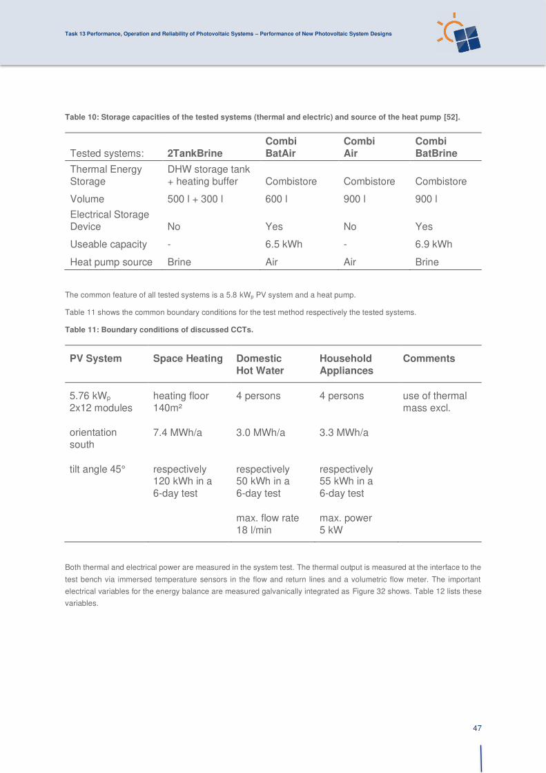
Task 13 Performance, Operation and Reliability of Photovoltaic Systems – Performance of New Photovoltaic System Designs
47
Table 10: Storage capacities of the tested systems (thermal and electric) and source of the heat pump [52].
Tested systems: 2TankBrine Combi BatAir
Combi Air
Combi BatBrine
Thermal Energy Storage
DHW storage tank + heating buffer Combistore Combistore Combistore
Volume 500 l + 300 l 600 l 900 l 900 l
Electrical Storage Device No Yes No Yes
Useable capacity - 6.5 kWh - 6.9 kWh
Heat pump source Brine Air Air Brine
The common feature of all tested systems is a 5.8 kWp PV system and a heat pump.
Table 11 shows the common boundary conditions for the test method respectively the tested systems.
Table 11: Boundary conditions of discussed CCTs.
PV System Space Heating Domestic Hot Water
Household Appliances
Comments
5.76 kWp 2x12 modules
heating floor 140m²
4 persons 4 persons use of thermal mass excl.
orientation south
7.4 MWh/a 3.0 MWh/a 3.3 MWh/a
tilt angle 45° respectively 120 kWh in a 6-day test
respectively 50 kWh in a 6-day test
respectively 55 kWh in a 6-day test
max. flow rate 18 l/min
max. power 5 kW
Both thermal and electrical power are measured in the system test. The thermal output is measured at the interface to the
test bench via immersed temperature sensors in the flow and return lines and a volumetric flow meter. The important
electrical variables for the energy balance are measured galvanically integrated as Figure 32 shows. Table 12 lists these
variables.

Task 13 Performance, Operation and Reliability of Photovoltaic Systems – Performance of New Photovoltaic System Designs
48
Figure 32: Fixed (galvanically integrated) measuring points. In addition, non-contact measurements are carried
out within the tested system.
Table 12: Important electrical variables for the energy balance.
Variable Description
EPV-yield Produced PV electricity, measurement on the DC and AC lines; the AC current measurement is used for the energy balance.
EHH Household electricity (without heat pump).
Egrid-purchase Electric energy from the grid.
Egrid-feed-in Electric energy supplied to the grid.
Various key figures are determined from the measurement data of the system test. The self-consumption ratio (Rself-con,eq.
Erreur ! Source du renvoi introuvable.)) is the share of locally produced PV energy used on-site.
(26)
The degree of self-sufficiency Rsuff in eq. Erreur ! Source du renvoi introuvable. describes the level of independence
from the external power grid.

Task 13 Performance, Operation and Reliability of Photovoltaic Systems – Performance of New Photovoltaic System Designs
49
(27)
The PV generation ratio (Rgen, eq. Erreur ! Source du renvoi introuvable.) describes the ratio of PV yield to total electrical
energy consumption. A system with Rgen = 1 corresponds to a net-zero energy building. Due to the different efficiencies of
the different systems tested and thus different values for the total energy consumption (Econsumption), the PV generation ratio
can vary despite the same size of PV system and the same useful energy demand in terms of heat for space heating and
DHW and electricity for the household.
(28)
The grid purchase ratio (Rnet, eq. Erreur ! Source du renvoi introuvable.)) describes the ratio of energy purchased from
the grid to total useful energy demand (Euse) for household electricity, domestic hot water (QDHW) and space heating (QSH,
eq. Erreur ! Source du renvoi introuvable.)). In this way, a mixed calculation of thermal and electrical energy is used.
The advantage, however, is that all variables are defined by the test method and are identical for all tests.
(29)
(30)
4.3.3 System test and results
The installation of the systems on the test bench includes all hydraulic components as well as a complete electrical
installation to supply the building with electricity. The tested systems had to work autonomously to meet the building's heat
and electricity requirements. This also includes determining the current surplus of PV electricity and a strategy to utilize
this energy.
The systems that were tested aimed to increase self-sufficiency and decrease electricity costs for the household. This was
done by a smart handling of the PV surplus and the storage capacities available in the system.
Figure 33 shows the PV yield and PV surplus, which are identical to all systems since they are the result of the yield that
is predefined by the PV plant and weather and the equally predefined household electricity consumption (without heat
pump). In the evaluation shown, the surplus is calculated on a per-minute basis, and shows the potential that is available
for increasing self- consumption. Figure 34 shows how much of this PV surplus was fed to the grid by the different systems
that were tested. Figure 35 shows the electric energy consumption from the grid for the same systems. Within the four
tested Systems the CombiBatBrine-System uses the least electricity from the grid (45 kWh in total, Figure 35). Due to the
test method, the loads of space heating, domestic hot water and household electricity are equal for all systems. For this
reason, the key figures of the tested systems can be compared directly with each other.

Task 13 Performance, Operation and Reliability of Photovoltaic Systems – Performance of New Photovoltaic System Designs
50
Figure 33: PV yield and household electricity and PV surplus per day. The calculation of PV surplus is based on
minutes.
The CombiBatBrine-System reaches in all categories shown in Figure 36 the best value. For the Key Performance
Indicators (KPIs) self-consumption, self-efficiency and PV generation (grey to black bars) a higher value is better, for the
grid purchase ratio (green bars) a lower value is better. The CombiBatAir-System achieves a comparatively high self-
consumption ratio. However, the self-consumption ratio increases with higher overall consumption, and the purchase of
electricity from the grid was thus also highest for the CombiBatAir-System, which shows the weakness of self-consumption
and self-sufficiency as KPIs. The PV generation ratio can vary despite an identical PV system and identical useful energy
demand. The CombiBatBrine-System achieves the highest yield ratio due to its lowest total consumption. A PV generation
ratio of 1 indicates a Net Zero Energy building. In this case, internal consumption and self-sufficiency must be identical.
Figure 34: Electric energy supplied to the grid per day.
Figure 36 shows the key performance factor grid purchase ratio. It shows what proportion of total useful energy demand
(the addition of DHW delivered, space heat delivered, and household electricity) had to be covered by electricity from the
grid. This value should be as low as possible. The System CombiBatBrine achieves the lowest and thus the best value. A
grid purchase ratio of 20% means that compared to the total useful energy demand, only 20% of electricity input from the
grid was necessary. In other words, the system delivered five times more useful energy than it consumed electricity from
the grid.
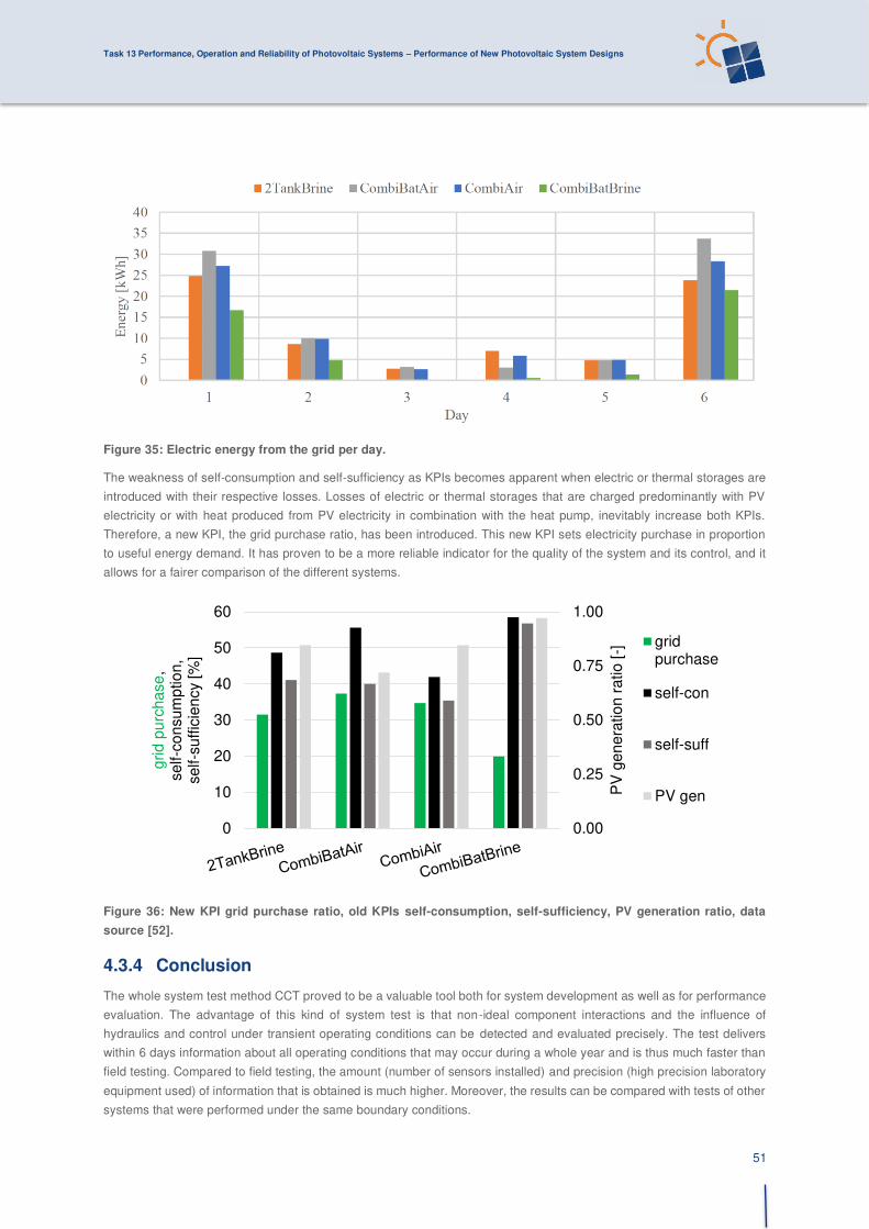
Task 13 Performance, Operation and Reliability of Photovoltaic Systems – Performance of New Photovoltaic System Designs
51
Figure 35: Electric energy from the grid per day.
The weakness of self-consumption and self-sufficiency as KPIs becomes apparent when electric or thermal storages are
introduced with their respective losses. Losses of electric or thermal storages that are charged predominantly with PV
electricity or with heat produced from PV electricity in combination with the heat pump, inevitably increase both KPIs.
Therefore, a new KPI, the grid purchase ratio, has been introduced. This new KPI sets electricity purchase in proportion
to useful energy demand. It has proven to be a more reliable indicator for the quality of the system and its control, and it
allows for a fairer comparison of the different systems.
Figure 36: New KPI grid purchase ratio, old KPIs self-consumption, self-sufficiency, PV generation ratio, data
source [52].
4.3.4 Conclusion
The whole system test method CCT proved to be a valuable tool both for system development as well as for performance
evaluation. The advantage of this kind of system test is that non-ideal component interactions and the influence of
hydraulics and control under transient operating conditions can be detected and evaluated precisely. The test delivers
within 6 days information about all operating conditions that may occur during a whole year and is thus much faster than
field testing. Compared to field testing, the amount (number of sensors installed) and precision (high precision laboratory
equipment used) of information that is obtained is much higher. Moreover, the results can be compared with tests of other
systems that were performed under the same boundary conditions.
0.00
0.25
0.50
0.75
1.00
0
10
20
30
40
50
60P
V g
ener
atio
n ra
tio [-
]
grid
pur
chas
e,se
lf-co
nsum
ptio
n,se
lf-su
ffici
ency
[%]
gridpurchase
self-con
self-suff
PV gen

Task 13 Performance, Operation and Reliability of Photovoltaic Systems – Performance of New Photovoltaic System Designs
52
The CCT protocol proves that the grid purchase ratio assesses also for losses in PV and heating systems as combined
systems which are ignored by other often used performance factors.
4.4 Performance of PV storage systems
4.4.1 State-of-the-Art – Performance testing of PV storage systems
The state of the art for efficiency assessment of PV storage systems, is given by the German “Efficiency guideline for PV storage systems”, published by the German Energy Storage Association (BVES) and German Solar Industry Association BSW) first in April 2017 and in English language in April 2019 [43]. It addresses performance testing of the power
conversion system, the battery and the control system. Despites the guideline also the international IEC 61427-2:2015
standard (Secondary cells and batteries for renewable energy storage - General requirements and methods of test - Part
2: On-grid applications) [53] includes methods for testing the battery roundtrip efficiency. As the power conversion and
control system is not addressed its applicability for PV storage systems is limited. The IEC 62933-2-1 (Electric energy
storage (EES) systems - Part 2-1: Unit parameters and testing methods - General specifications) [54] provides simple test
procedures for determination of the roundtrip efficiency and usable energy of electrical energy storage systems at the AC-
connection point. The standard is limited applicable for DC-coupled systems, which are charging the battery directly from
PV and not from the AC connection point.
Further efforts in standardization for residential storage systems are expected in Australia within the frame of a funded
project by the Australian Renewable Energy Agency (ARENA lead by DNV GL. In Germany the working group AK 371.0.9
of the DKE (German Commission for Electrical, Electronic & Information Technologies) started 2019 its work for future
standardization of key performance indicators of stationary battery storage systems.
4.4.2 Characteristics of PV storage systems
PV storage systems can be characterized by their power and capacity rating but also by their specific system topology as
AC and DC coupled, single phase, three phase systems or low-voltage and high voltage battery system. A classification
can be done according to the following specifications:
Table 13: PV battery storage system classification.
Connection scheme
Topology (AC or DC coupled) Phases (single phase or three phase)
Power rating
Maximum PV input power in case of a DC coupled system
Maximum output power (battery discharge and PV feed in)
Storage specifications
Low voltage or high voltage battery system Charge / discharge power or relation between power and capacity similar to the C-Rate
Battery capacity
Usable energy of the battery, dischargeable with a certain power from the battery
Usable energy of the system, which can be discharged at the AC connection point of the system (battery capacity reduced by inverter losses for a certain power level).
Two main system topologies, the AC and DC coupled system, exist. The principle of the AC coupled system is illustrated
in Figure 37. The battery is connected over a bidirectional inverter to an AC connection point in the household. The DC
coupled system is shown in Figure 38. The battery and PV array are connected to the DC-link (intermediate circuit) of the

Task 13 Performance, Operation and Reliability of Photovoltaic Systems – Performance of New Photovoltaic System Designs
53
inverter. For the DC coupled system also a special type, the PV generator coupled system exists, which connects the
battery over a converter directly to the PV array and a conventional PV inverter.
Figure 37: Test setup for an AC coupled system [43].
AC coupled and PV generator coupled systems are retrofittable and can be added to installations with conventional PV
systems. An advantage of the AC coupled system is that the power rating of the battery inverter can be sized independently
from the PV system size. This is usually not the case for DC coupled systems with a hybrid inverter. A smaller power of
the battery inverter can be beneficial due to higher efficiencies in partial load operation and lower standby-losses under
the assumption that most of the time the discharge power is below a certain level in residential homes. An advantage of
the DC coupled system is that for battery charging no DC to AC conversion of the PV inverter and additional AC to DC
conversion of the battery inverter is necessary. Hence, energy losses for charging are typically reduced.

Task 13 Performance, Operation and Reliability of Photovoltaic Systems – Performance of New Photovoltaic System Designs
54
Figure 38: Test setup for an DC coupled system [43].
4.4.3 Efficiency assessment according to the BVES/BSW efficiency guideline for PV storage systems
The efficiency guideline provides test procedures for the efficiency assessment of the main three subsystems of PV storage
systems.
• Power conversion system
• The battery system
• Performance of the control system.
The test setup for AC and DC coupled system corresponds to Figure 37 and Figure 38. The tests require adjusting a
certain charge / discharge or grid-feed in power at a certain State of Charge (SOC) of the battery, which is done by
controlling the PV power of a PV-Emulator and power of an adjustable load. For a sub clause of tests, it is also allowed to
adjust power set points over a communication interface as Modbus e.g. Sunspec [43].
4.4.4 Power conversion system
Efficiency evaluation of the power conversion system determines the energy conversion losses and the standby
consumption of the power converters. For PV storage systems different energy conversion paths can be distinguished.
They are shown in Figure 39 for the different system topologies.
• PV direct grid feed-in
• Battery charging
• Battery discharging

Task 13 Performance, Operation and Reliability of Photovoltaic Systems – Performance of New Photovoltaic System Designs
55
Figure 39: Energy conversion pathways of the individual topologies of PV storage systems [43].
For each energy conversion path, the efficiency is determined at full and partial load condition (100%, 75%, 50%, 30%,
25%, 20%, 10%, 5% of nominal power). For the AC- and PV-generator coupled system it is not necessary to measure
also the efficiency of the PV inverter, which is usually a third-party device.
The standby consumption of the power conversion equipment is determined for a fully discharged (typically at the morning
hours) and fully charged battery (typically the hours before sunset). The energy can be provided from the battery or AC
grid if charged and must be provided from the AC grid when the battery is discharged.
4.4.5 Battery
The test procedure addresses the round-trip efficiency and net capacity of the battery. It is determined by fully discharging
and recharging the battery several times (full cycles). The battery efficiency is the ratio between discharged to charged
energy. The net capacity corresponds to the discharged energy. The efficiency is determined for 100%, 50% and 25% of
nominal power and for each power level three full charge/discharge cycles are required.
4.4.6 Control system
The main objective of residential PV battery systems is to increase the self-sufficiency in homes. The basic control strategy
is to reduce grid consumption and grid feed-in at the GCP to zero. It is done by charging the battery if PV generation is
higher than the load demand (surplus) and discharging when the PV production is lower than the load demand (deficit). A
surplus requires to feed-in the additional power to the utility grid, a deficit to import power from the utility grid. For most
systems an AC energy meter is used at the GCP, which sends this information to the energy management system (EMS)
of the PV storage system. The EMS starts to control the battery power to reduce the grid power to zero by charging the
battery at a PV surplus and discharging it at a PV deficit. Limitations result due to the maximum charge/discharge power
and instantaneous SOC. As an alternative to the energy meter at the GCP some systems use current transducers at the
load and PV inverter output to measure the electric demand and generation for controlling the battery power.
The dynamic behaviour is limited due to delays in the control loop as maximum data exchange speed from the energy
meter to the EMS and the time period for the active power calculation. Hence the battery power is not adjusted-, and grid
power is not reduced immediately after changes in PV generation or load demand. Furthermore, the energy measurement
at the GCP to the utility grid has a certain accuracy and resolution. Because of this a state error may result and the grid
power is not reduced completely to zero.
The object of investigation is to test the speed and accuracy of the control system as important performance indicator. For
assessment of the dynamic control behaviour in total 140 load steps are performed. Figure 40 shows the response of a
tested PV battery storage system to one of the 140 load steps. The delay time td = t2 until the battery power starts to
increase and the settling time ts = t1-t3 until the battery power reaches and stays within a ± 5% tolerance band of the end
value at which grid power is reduced best possible to zero. Evaluation of the steady state error is also done for several
load steps and the deviation to zero grid power measured.

Task 13 Performance, Operation and Reliability of Photovoltaic Systems – Performance of New Photovoltaic System Designs
56
Figure 40: Determination of the dead td and settling time ts according to the BVES / BSW efficiency guideline [43].
4.4.7 Test results of battery storage systems according to the BSW/BVES efficiency guidelines
Within the “Energy Storage Inspection 2020” of the HTW Berlin [55] several manufacturers tested their system according
to the efficiency guidelines and provided test results for the study. A brief overview of the results is given within this section.
In Figure 41 the discharge efficiency of the battery inverter for the tested AC coupled systems is shown in an efficiency
chart.
Figure 41: Efficiency chart for battery discharge BAT2AC for AC coupled systems [55].
Table 14 lists the measured efficiency as the average over the eight tested power levels for each energy conversion path.

Task 13 Performance, Operation and Reliability of Photovoltaic Systems – Performance of New Photovoltaic System Designs
57
Table 14: Average efficiency of nine AC coupled and seven DC coupled systems under test, based on “Energy Storage Inspection 2019” of the HTW Berlin [55].
System or Config
PV- grid feed in
PV battery charge
AC battery charge
AC battery discharge
10 AC systems
Min.: Not required for this topology 91.7% 92.0%
Median: 93.5% 93.7%
Max.: 95.1% 95.4%
11 DC systems
Min.: 95.1% 89.6% 95.7% 90.3%
Median: 96.1% 95.5% 95.9% 95.2%
Max.: 97.6% 98.2% 96.9% 97.3%
Results for the battery round-trip efficiency from the Energy Storage Inspection 2019 are given in Table 15. The efficiency
of the tested systems is between 91% and 97%. The charge/discharge power of the test is related to the nominal power
of the system. As each system has its individual power the batteries were not charged and discharged with the same
power/capacity ratio for a direct comparison e.g. which battery cell performs better. The battery cell efficiency usually
increases with lower power/capacity rates due to lower thermal losses.
Table 15: Average battery efficiency (mean of 100%, 50%, 25% nominal power) for different systems [56].
System A1 A2 A3 A4 B1 C1 C2 D1 D3 D4 D5 D6
ηSys [%] 94.8 94.5 91.5 96.3 96.9 98.0 98.0 94.8 95.3 94.8 95.3 95.3
System D7 E1 E2 F2 G1 H1 I1
ηSys [%] 95.2 92.6 95.6 94.7 96.1 94.6 87.9
The time it takes until the battery power is increased after a load step (dead time) is determined for the tested systems
between < 0.4 and 2 seconds. The settling time until the battery power is in a steady-state (± 5% of end value) is between
0.4 and 13 seconds.
The introduced measurement process provides reliable figures regarding battery system properties. They can be used as
input parameters for battery system simulations of individual use cases, which can provide meaningful performance
indicators as they are described in the next two section. A current research project conducts further tests and development
of the measurement protocol of the efficiency guideline with the aim to start a standardization process [57].
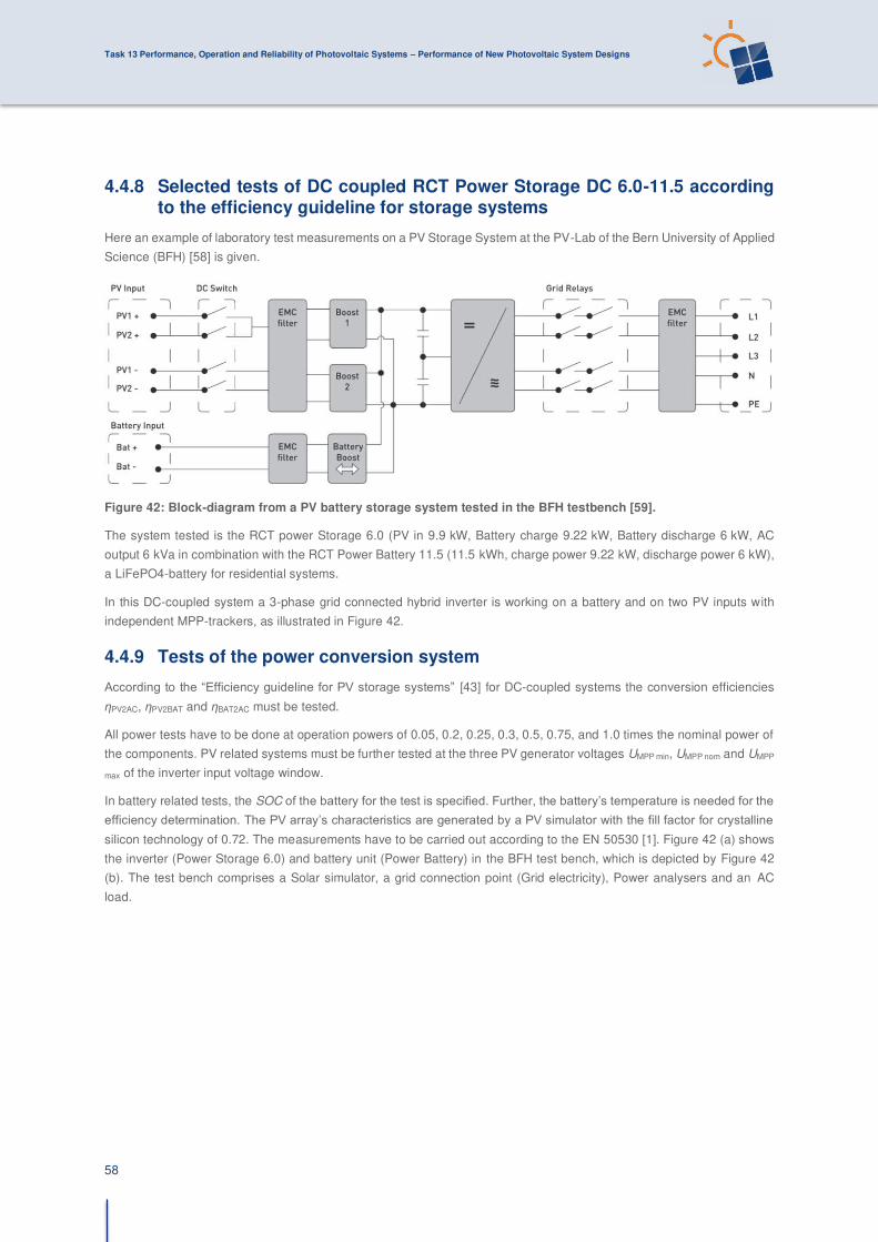
Task 13 Performance, Operation and Reliability of Photovoltaic Systems – Performance of New Photovoltaic System Designs
58
4.4.8 Selected tests of DC coupled RCT Power Storage DC 6.0-11.5 according to the efficiency guideline for storage systems
Here an example of laboratory test measurements on a PV Storage System at the PV-Lab of the Bern University of Applied
Science (BFH) [58] is given.
Figure 42: Block-diagram from a PV battery storage system tested in the BFH testbench [59].
The system tested is the RCT power Storage 6.0 (PV in 9.9 kW, Battery charge 9.22 kW, Battery discharge 6 kW, AC
output 6 kVa in combination with the RCT Power Battery 11.5 (11.5 kWh, charge power 9.22 kW, discharge power 6 kW),
a LiFePO4-battery for residential systems.
In this DC-coupled system a 3-phase grid connected hybrid inverter is working on a battery and on two PV inputs with
independent MPP-trackers, as illustrated in Figure 42.
4.4.9 Tests of the power conversion system
According to the “Efficiency guideline for PV storage systems” [43] for DC-coupled systems the conversion efficiencies
ηPV2AC, ηPV2BAT and ηBAT2AC must be tested.
All power tests have to be done at operation powers of 0.05, 0.2, 0.25, 0.3, 0.5, 0.75, and 1.0 times the nominal power of
the components. PV related systems must be further tested at the three PV generator voltages UMPP min, UMPP nom and UMPP
max of the inverter input voltage window.
In battery related tests, the SOC of the battery for the test is specified. Further, the battery’s temperature is needed for the efficiency determination. The PV array’s characteristics are generated by a PV simulator with the fill factor for crystalline
silicon technology of 0.72. The measurements have to be carried out according to the EN 50530 [1]. Figure 42 (a) shows
the inverter (Power Storage 6.0) and battery unit (Power Battery) in the BFH test bench, which is depicted by Figure 42
(b). The test bench comprises a Solar simulator, a grid connection point (Grid electricity), Power analysers and an AC
load.

Task 13 Performance, Operation and Reliability of Photovoltaic Systems – Performance of New Photovoltaic System Designs
59
(a)
(b)
Figure 42: (a) Power Storage DC 6.0-11.5 during the tests, (b) Simulation and measurement test bench for PV
battery storage systems at BFH.
In this DC-coupled system a 3-phase grid connected hybrid inverter is working on a battery and on two PV inputs with
independent MPP-trackers, as can be seen in Erreur ! Source du renvoi introuvable..
4.4.10 Results of the conversion efficiencies tests
In Figure 43 (a)-(c) the results for the conversion efficiencies PV2AC, PV2BAT and BAT2AC are given. The three lines in
PV2AC and PV2BAT represent the total conversion efficiencies for the three specified operation voltages UMPP min = 290 V,
UMPP nom = 700 V, UMPP max = 780 V of the inverter as a function of the predefined relative power levels. In the test UMPP max
was set at 780 V instead of 800 V, due to a limitation of the test infrastructure.
(a)
(b)
(c)
POWERBATTERY11.5 kWh
Solar simulator
AC loadGrid electrcity
Poweranalyzers

Task 13 Performance, Operation and Reliability of Photovoltaic Systems – Performance of New Photovoltaic System Designs
60
Figure 43: Path conversion efficiencies of the tested PV battery storage system (a) PV2AC, (b) PV2BAT and (c)
BAT2AC.
The total efficiency ηPV2AC (PV grid feed-in and direct use efficiency) had to be determined at the nominal power of 6 kW.
During the test the battery was fully charged. The total efficiency ηPV2BAT was tested at the nominal power of 9.9 kW for
UMPP nom and UMPP max and at 6 kW for UMPP min. During the test SOC was 55% +/- 10%. The efficiency ηBAT2AC was
determined at the nominal power of 6 kW. During the test SOC was 55% +/- 10%
4.4.11 Battery efficiency
The efficiency of batteries varies depending on their charging and discharging power. In a full cycle the battery is fully
discharged by setting a constant load (grid-feed-in while zero generation) and then fully charged again by setting a constant
generation and zero load consumption.
Table 16: Operating points for the pathways BAT2AC and PV2BAT [43].
Power cycle 1 Power cycle 2 Power cycle 3
Discharge power PBAT2AC,nom 0.5*PBAT2AC,nom 0.25*PBAT2AC,nom
Charging power PPV2BAT,nom 0.5*PPV2BAT,nom 0.25*PPV2BAT,nom
Iterations 3 3 3
The efficiency of a full cycle is determined by the ratio between the energy supplied and the energy withdrawn on the DC
side. The battery efficiency tests have to be done for three iterations for three different powers in charge and discharge
(power cycles 1 to 3) which depend on the nominal battery charging and discharging power as can be seen in Table 16.
4.4.12 Results of the battery efficiency tests
The battery was tested between system SOCmin = 5% and SOCmax = 97%. Because the maximal battery charge and
discharge power are different for this battery, six different power levels have to be applied in the test.
In Figure 44 the charge and discharge power as a function of time is shown for the three power cycles or six half power
cycles of the second iteration. From the integrated power over time of the two half power cycles the energies are
determined, and the efficiency of a full power cycle is calculated.

Task 13 Performance, Operation and Reliability of Photovoltaic Systems – Performance of New Photovoltaic System Designs
61
Figure 44: Charge and discharge power curves as a function of time for the six half cycles of the second iteration.
For each of the three cycles the charged and discharged energies and cycle efficiency values are given.
4.4.13 No-load and standby losses
The no-load consumption is measured when the battery is at SOCmax and SOCmin by switching off the load and PV
generator. To measure the standby consumption, the conditions specified by the manufacturer for transition to standby
mode are established.
The loss of the system is also measured when it is switched off. For this purpose, the system is deactivated according to
the manufacturer's specifications and the energy consumption is measured. This is only done at maximum battery
capacity.
For the tested system the losses have been measured at SOCmin = 7% and SOCmax = 97%. In Erreur ! Référence non
valide pour un signet. the measured losses are given.
The chapters Erreur ! Source du renvoi introuvable. to Erreur ! Source du renvoi introuvable. show the general
approach and the test protocols of the BVES / BSW efficiency guideline and give a broad overview of test results of battery
storage systems according to the efficiency guidelines. Besides this overview the sections Erreur ! Source du renvoi
introuvable. to Erreur ! Source du renvoi introuvable. show the test protocols and measured data for a single battery
storage to give detailed insights into the results a test according to the BVES / BSW efficiency guideline provides.
0
1000
2000
3000
4000
5000
6000
7000
8000
9000
10000
0:00 1:00 2:00 3:00 4:00 5:00 6:00 7:00 8:00 9:00 10:00
Pow
er [W
]
Time [h]
Charged and discharged Energy at the second iteration
Discharging PowerCharging Power
Charged Energy: 11.296 kWh
Discharged Energy: 10.627 kWh
Charged Energy: 11.188 kWh
Discharged Energy: 10.713 kWh
Charged Energy: 10.781 kWh
Discharged Energy: 11.149 kWh
Power Cycle 1 Efficiency = 94.078%
Power Cycle 2 Efficiency = 95.754%
Power Cycle 3 Efficiency = 96.699%

Task 13 Performance, Operation and Reliability of Photovoltaic Systems – Performance of New Photovoltaic System Designs
62
Table 17: No-load and standby losses at different battery charge states.
Losses SOCmax SOCmin
No-load No-load Stand-by
PBAT2AC in W 23.91 18.89 5.76
PGrid (Purchase) in W 2.57 6.3 0.1
4.5 Performance indices for parallel agricultural and PV usage
Scarcity of land remains an arguable issue when comparing the performance of PV with other power generating
technologies. In densely populated countries, particularly, the vast potential of utility scale ground-mounted PV (GM-PV)
together with its large land use footprint is frequently discussed.
Figure 45: Illustration of an APV system with different utilization options for the produced electricity.
One approach of minimizing the land use footprint of GM-PV is agrivoltaics (APV), a dual use of land for food production
and PV power generation [58]. While Goetzberger and Zastrow developed the concept already back in 1981 [59], today,
APV gains in attention and political support in a growing number of countries accompanied by notable research activities
in France, USA and Korea, amongst others.
4.5.1 Measuring land use efficiency of agrivoltaics
To quantify land use efficiency of intercropping systems, Mead and Willey [60] introduced the concept of the Land
Equivalent Ratio (LER), which is frequently applied in agroforestry, aquaponics, and recently also APV [61].
The LER can be defined as the relative land area that is required for mono-production in order to achieve the yield of dual
land use. Following Willey [62], the LER is specified as the sum of the respective yield ratios of dual land use to mono land
use:

Task 13 Performance, Operation and Reliability of Photovoltaic Systems – Performance of New Photovoltaic System Designs
63
(31)
For APV systems, a and b represent the cultivated crop and generated electricity, respectively. In field experiments, crop
yields are typically measured comparing the yield of several test plots below the APV system with reference fields without
shading from APV structures. Therefore, another factor to be considered is the land losses (LL) that occur if a part of the
land cannot be cultivated due to the mounting structure of the APV system. When larger land machines are employed, LL
are usually much larger than the built-up area itself.
(32)
A LER < 1 indicates that combined crop and energy production is less productive than separate production, whereas a
LER > 1 indicates increased productivity in the APV system as compared to mono production.
4.5.2 Land equivalent ratio of Fraunhofer ISE pilot system near Lake Constance
In 2016, Fraunhofer ISE installed Germany’s largest APV research facility near Lake Constance with a capacity of 194.4 kWp. Experiments were deducted over a crop rotation of potato, celery, clover grass, and winter wheat. In the first
year, the average results amounted to approximately 20% lower yields for both the agricultural and electrical layer leading
to a LER of 1.6 or a rise of land use efficiency of 60% which is illustrated in Figure 46.
Since the installation of the pilot plant, with 1.87 the highest LER was observed in the dry and hot summer 2018 for celery,
which indicated a 12% rise of yield compared to the reference area.
Regarding the electrical performance of the APV system, ZENIT, a software tool developed by Fraunhofer ISE [63], was
employed to simulate the overall electrical yield of a standard GM-PV system implementing a chain of loss models. With
78.1 kWp/m², the installed capacity of the reference scenario was 39% higher compared to the capacity of the APV system.
Due to the application of bifacial modules in the APV system, though, the measured field results of the APV system were
only 17% below the simulated results of the GM-PV system.
Regarding additional land losses of the mounting structure, only 0.23% of the total area was covered by mounting structure
elements, whereas real LL amounted to 8.3% of the total area. Accordingly, the LER of celery in 2018 can be calculated
as
(33)
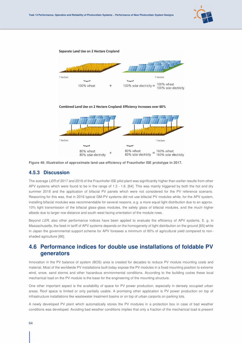
Task 13 Performance, Operation and Reliability of Photovoltaic Systems – Performance of New Photovoltaic System Designs
64
Figure 46: Illustration of approximate land use efficiency of Fraunhofer ISE prototype in 2017.
4.5.3 Discussion
The average LER of 2017 and 2018 of the Fraunhofer ISE pilot plant was significantly higher than earlier results from other
APV systems which were found to be in the range of 1.3 - 1.6. [64]. This was mainly triggered by both the hot and dry
summer 2018 and the application of bifacial PV panels which were not considered for the PV reference scenario.
Reasoning for this was, that in 2016 typical GM-PV systems did not use bifacial PV modules while, for the APV system,
installing bifacial modules was recommendable for several reasons, e.g. a more equal light distribution due to an approx.
10% light transmission of the bifacial glass-glass modules, the safety glass of bifacial modules, and the much higher
albedo due to larger row distance and south-west facing orientation of the module rows.
Beyond LER, also other performance indices have been applied to evaluate the efficiency of APV systems. E. g. in
Massachusetts, the feed-in tariff of APV systems depends on the homogeneity of light distribution on the ground [65] while
in Japan the governmental support scheme for APV foresees a minimum of 80% of agricultural yield compared to non -
shaded agriculture [66].
4.6 Performance indices for double use installations of foldable PV generators
Innovation in the PV balance of system (BOS) area is created for decades to reduce PV module mounting costs and
material. Most of the worldwide PV installations built today expose the PV modules in a fixed mounting position to extreme
wind, snow, sand storms and other hazardous environmental conditions. According to the building codes these local
mechanical load on the PV module is the base for the engineering of the mounting structure.
One other important aspect is the availability of space for PV power production, especially in densely occupied urban
areas. Roof space is limited or only partially usable. A promising other application is PV power production on top of
infrastructure installations like wastewater treatment basins or on top of urban carports on parking lots.
A newly developed PV plant which automatically stores the PV modules in a protection box in case of bad weather
conditions was developed. Avoiding bad weather conditions implies that only a fraction of the mechanical load is present

Task 13 Performance, Operation and Reliability of Photovoltaic Systems – Performance of New Photovoltaic System Designs
65
on the PV modules and the structure, enabling light weight structural design. First patents were filed in 2012 [67] and first
results of the URBAN PLANT prototypes were presented in 2013 at the European PV conference [68].
(a)
(b)
Figure 47: The DHP’s 640 kW HORIZON solar foldable PV plant on top of the wastewater retreatment basins in
Chur, Switzerland operating since (Source: dhp technology AG).
This newly developed PV plant folding the PV generator into a protection box and will pull out the PV generator, carried
on supporting cables for operation during good weather conditions. An innovative autonomous control system to trigger
the folding process was developed based on local meteo sensors and regional weather information.
Figure 48: Parts of the PV foldable roof is opened to get access to regular service activities concerning the
infrastructure of the wastewater treatment system (Source: dhp technology AG).
The DHP Horizon system Chur (Figure 47 -Figure 49) consists of crystalline silicon PV generators grouped in sectors of
13 kWp each, moved by a single traction AC drive. This sub generator is segmented in forty 72 silicon 6” cells PV modules moulded in a glass fibre reinforced plastic mounting. Each 13 kWp generator is moved a single AC motor into the safety
box by a steering cable if automatically if the wind speed exceeds 15 m/s. In most of the regions in Switzerland this heavy
wind will lead to PV performance losses of below 3% relative to a fixed PV installation [68].The manufacturer guarantees
operation lifetime of 25 years for the PV generator in this application and 40,000 cycles of moving the folding system
corresponding to roughly four movements a day.
(a) (b)

Task 13 Performance, Operation and Reliability of Photovoltaic Systems – Performance of New Photovoltaic System Designs
66
Figure 49: View of the HORIZON PV plant on top of the filled basins (left) and (right) the cleaning of the basins
during regular service activities. (Source: dhp technology AG)
Figure 50: The measured yield of HORIZON 640 kW in Chur was at specific 900 kWh/kWp and +/- 3% of similar
fixed mounted horizontal PV plant close by in Chur [69].
The PV Horizon installation in Chur supplies about 20% of the total electricity needs of the wastewater treatment facility
with a 95% PV self-consumption rate.
Beside the solar electricity supply the most valuable benefit in the wastewater system operation is the highly reduced
growth rate of algae. Due to the shading of the basins by the solar modules the cost of the annual cleaning process is
reduced. This is estimated to count for a financial benefit of about 0.02 €/kWh PV electricity produced.
In 2019 DHP has installed the first foldable HORIZON PV generator on top of a PV carport in Appenzell, Switzerland, see
Figure 51. This will lead again to the advantage of the double use of land for PV and car parking purposes together with
the shading effect for the car owners in summer time. Due to the reduced amount of used kg metal for the ground mounting
system, the linked CO2 emission of the BOS is drastically reduced compared to fixed PV module mounting solutions [68].
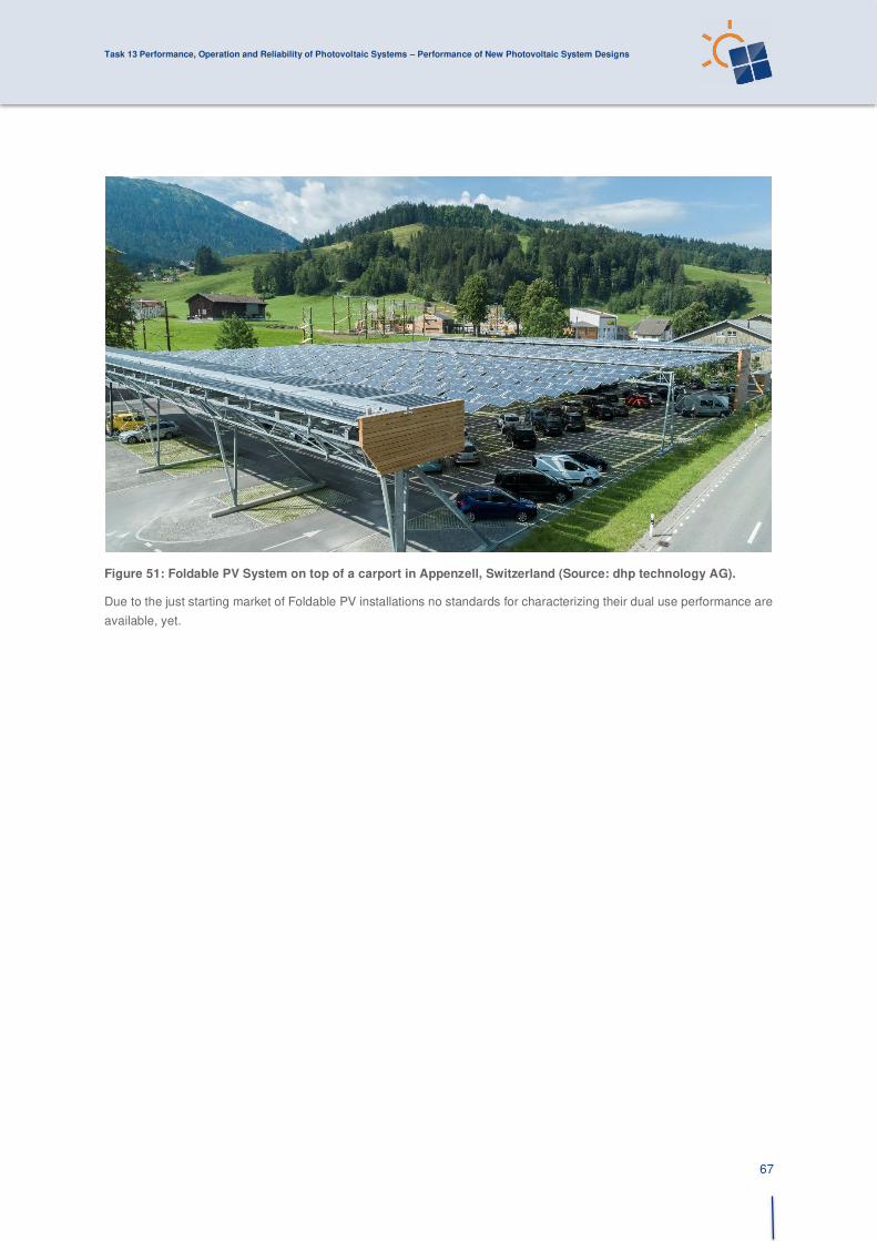
Task 13 Performance, Operation and Reliability of Photovoltaic Systems – Performance of New Photovoltaic System Designs
67
Figure 51: Foldable PV System on top of a carport in Appenzell, Switzerland (Source: dhp technology AG).
Due to the just starting market of Foldable PV installations no standards for characterizing their dual use performance are
available, yet.

Task 13 Performance, Operation and Reliability of Photovoltaic Systems – Performance of New Photovoltaic System Designs
68
5 PERFORMANCE OF SHOWCASES OF COMPLEX PV SYSTEMS WITH MULTIPLE FUNCTION
5.1 Performance of showcases of net integrated PV system with battery storage
5.1.1 Description of the showcase PV system
This showcase PV system is a hybrid generator comprising PV arrays, diesel generator, storage elements and a grid
connection. This type of system is very popular in developing countries and is reminiscent of the current trend towards PV
with storage coming of age in developed countries to alleviate stress on the distribution grid due to excessive PV
production. There is however a fundamental difference between the two applications, aside from the addition of the
generator, and that is the availability of the grid connection. The PV plus storage application in developed grid systems is
primarily grid connected, following the grid and reacting to grid fluctuations and events as a subordinate producer as per
the national and international standards for grid connected PV systems. Our showcase application is the opposite. The
primary energy producer is the PV system with a generator backup, the grid connection is secondary and used on rare
occasions when it is available and stable.
This particular system was built for a field school operating in a remote area unserved by the national utility in a developed
country. It is designed to receive a grid connection, though the grid has yet to reach the field school.
The school is comprised of two classroom complexes with LED tube lighting, air-conditioning units, computer and
projection equipment, coffee corner, restrooms and all the amenities one would expect of a modern educational
installation. There are also three small apartment dwellings for teaching staff on site. These dwellings are outfitted as
would be expected on any residential campus, with kitchen appliances, small air-conditioning units and household
electronics.
The load profile developed for an average 24-hour period with seasonal allowance shows that the primary load is applied
during the day light hours by the classrooms, while the residential loads are primarily drawn after the classrooms are shut
down for the day.
Our system is comprised of the following generator components:
• 40.5 kWp of solar PV modules installed on 4 separate roof surfaces
• 35 kVA diesel generator
• 2,500 Ah of flooded lead acid batteries
The components that integrate the system include:
• Hybrid inverters
• Battery chargers
• Solar inverters
The heart and brain of the system is the hybrid inverter. This element faces the electrical distribution panel of the consumer
and feeds the required energy on demand. The backend of the hybrid inverter receives the power inputs from the various
generators.
The PV modules are divided into two groups. Since the major component of the load is during the daylight hours when the
solar PV is working, most of the array is AC coupled directly into the consumer electric panel by a standard solar inverter
programmed for grid connection, in parallel with the hybrid inverter. When the solar energy produced is greater than the
consumption, the excess energy finds its way through the hybrid inverter to charge the battery bank.

Task 13 Performance, Operation and Reliability of Photovoltaic Systems – Performance of New Photovoltaic System Designs
69
If the batteries are charged, and excess power is flowing, the hybrid inverter raises the frequency of the system such that
the solar inverters will reduce production using a simple control loop supported by the solar inverter software system.
A small 6.5 kWp array, about 15% of the total, sized for the night load, is DC coupled to the hybrid inverter by way of a
battery charger. This small array is sized to charge the batteries during the day for use during the night while the AC
coupled array feeds the main load. The DC coupled array is also necessary to enable a black start of the system in such
a situation where there is no grid and no diesel fuel. The solar inverters are grid standard and will not operate in an island
mode. For the solar inverters to operate after a total shutdown, the DC coupled array is necessary to energize the hybrid
inverter and enable the solar inverter to couple with the load.
The division of the solar array between AC and DC coupling saves a lot of energy otherwise lost converting in two
directions. In the case of the AC coupling, the only loss of conversion efficiency is in the solar inverter as it inverts the PV
module DC power directly into the consumer electrical distribution panel. The DC coupled array would pass through the
charger, the battery and the hybrid inverter with losses at each stage.
Figure 52: System layout of PV hybrid show case with PV, diesel generator, battery and grid connection.
When battery charge drops below the designated critical level, the diesel generator is automatically actuated by the hybrid
inverter. Generator actuation automatically disconnects the solar array from feeding the consumer panel since a generator
of this size as compared to the PV array cannot easily fill in the variable PV energy flow. Figure 52 shows the complete
PV hybrid system topology with all components introduced before.
A grid connection in this configuration would require an anti-islanding mechanism that would cut out the PV generator
when the grid connection switch is closed and the grid parameters stray from the utility’s standard requirements for power quality. The diesel generator will never be enabled to run when the grid switch is closed.
The system modes of operation are as follows:
1. PV array – DC coupled array charges the batteries, the AC coupled array feeds the load with excess power
sent to charge batteries in parallel to the DC coupled charger. When batteries are full, DC coupled array
maintains trickle charge while the AC coupled array continues to feed the load regulating power production in
relation to the load by responding to varying frequency controlled by the hybrid inverter. The batteries feed the
load after sundown and during the day if the AC coupled array is unable to meet the demand.

Task 13 Performance, Operation and Reliability of Photovoltaic Systems – Performance of New Photovoltaic System Designs
70
2. Battery Mode – As night falls, the batteries begin to supply the load in parallel to the AC coupled array, taking
over fully as the array shuts down for the night. The battery bank is the sole power supply during the dark
hours, until the charge obtained during the day is exhausted due to low solar irradiation earlier in the day or
due to the connection of additional unauthorized load. At that point the system goes to diesel generator mode.
3. Diesel generator - During cloudy seasons, if the AC coupled array does not satisfy the load and at night when
there is no solar radiation, if the load is increased beyond the design threshold levels, the diesel generator will
automatically switch on and the AC coupled array will switch off. When batteries are fully charged the
generator switches off, the AC coupled array switch is reclosed and the diesel generator is switched off. The
diesel generator and the AC coupled PV array cannot work together.
4. Grid tied (designed, but not implemented due to lack of connection) – in this configuration. The grid supplies
the load in parallel with the AC coupled PV array while the small DC coupled array charges the batteries. If the
solar irradiation is not sufficient, to charge the batteries, the hybrid inverter connects grid power to the internal
charging unit. If the grid parameters fail to meet Power Quality criteria or drops out, the hybrid inverter opens
the grid Circuit Breaker to prevent PV energy from feeding the grid.
5.1.2 Qualifying performance
The focus of solar PV energy in developed countries for the most part has been maximizing system energy output through
increasing efficiency from the cell level down through the DC system, inverting process and grid connection. In an off-grid
system, the definition of performance has added dimensions. Conversion efficiency is only one area of performance that
must be considered. The defined purpose of system is not to achieve the highest energy yield possible with the chosen
components, but to ensure that the consumer is continuously supplied with quality electrical power. Achieving highest
energy yield possible is a performance metric, but only during the peak of the daily consumption and production cycle.
In a grid tied system, performance of the system is considered satisfactory if the performance meets the design criteria,
almost always defined as meeting the designed PR every month. In a hybrid system, the PR is of no consequence as an
ongoing performance qualifier, since the solar inverter coupled to the AC load and the solar charger coupled to the battery
bus-bar are regulated by demand, often curtailing even shutting down current flow in the system.
Upon completion of erecting any PV array a Performance Acceptance Test (PAT) is undertaken to ascertain that the
system is performing to specification and to set the baseline for future comparison. A grid connected PV array is tested
using the PR. In this test the array energy fed to the grid is compared to the solar energy absorbed by the modules as a
ratio. This PR is then compared to the theoretical PR calculated at the outset of the design process. The residual power
demand of the grid fed by the PV array is infinitely larger than the nominal power of the PV array itself, such that the grid
absorbs all the energy supplied.
In a hybrid system the feed in method is problematic since the power demand of the grid to be fed by the system is very
small. Its residual power demand is often less than the nominal power of the array. The PV array is often interrupted when
the batteries are full and the consumer demands less energy than the array is currently producing, rendering such a
method for defining the PV system efficiency as ineffectual.
The qualifying parameters in defining the performance of our system are the following:
• The straight-out PR of the system when consumption is at a maximum and the PV system is not being curtailed
• Number of battery system charging and discharging cycles
• Number of generator uptakes when batteries are exhausted
• Power quality in all modes of operation must be within the confines of internationally recognized parameters to
ensure that the consumer load will not be damaged. In a grid tied system, this is not a concern since the PV
system follows the grid. In this show case just, the PV systems sets up the grid by setting grid frequency and grid
voltage itself. The diesel generator never operates with the AC coupled PV.

Task 13 Performance, Operation and Reliability of Photovoltaic Systems – Performance of New Photovoltaic System Designs
71
5.1.3 Performance results
As discussed previously, the major performance matrix for a hybrid system in our configuration is uninterrupted power
supply to the load and battery charge cycling such that depth of discharge is within the design parameters.
In Figure 53 we see the correlation between the three main parameters for defining performance in our system – Load
consumption in kWh/d (red bars), PV production in kWh/d (yellow bars) and battery state of charge SOC in % (full blue
line). The dashed blue lines represent the minimum and maximum battery state of charge SOC measured during the
respective day.
Acceptable performance is defined as ensuring that the load is met while the SOC does not drop under the designed level
of 70%.
The graph shows the solar energy produced by the DC coupled PV array opposite the consumption drawn by the load
and in conjunction with the depth of discharge.
Performance in August is clearly high due to the solar resource available. The graph of December exhibits the challenge
of the design. The first week of the December seems to have been somewhat overcast and the battery discharges to the
lowest limit of the designed level. During the second week it appears that the clouds have moved on and the high levels
of solar energy in contrast to the consumption from the 11th to the 13th of the month manage to charge the batteries back
to maximum.
That the battery discharge level did not drop below the designed 70% during December is the most important performance
indicator. So, 100 % of the evaluated days (August and December) met the performance requirements.
(a)
(b)
Figure 53: Operating data of the PV hybrid system from (a) August and (b) December.
0102030405060708090100
0
50
100
Sta
te o
f Cha
rge
(SoC
) in
%
Ene
rgy
in k
Wh
Load consumptionPV productionSoC mean
0102030405060708090100
0
50
100
Sta
te o
f Cha
rge
(SoC
) in
%
Ene
rgy
in k
Wh
Load consumptionPV productionSoC mean

Task 13 Performance, Operation and Reliability of Photovoltaic Systems – Performance of New Photovoltaic System Designs
72
5.2 Performance of floating PV systems
Massive tracks of land are used in the development of large utility-scale PV system installations, yet the demand for more
solar energy continues to grow. Future large developments could be limited due to the cost and availability of land, [70]–[72]. This has prompted the development of floating PV systems (FPV), both on-shore, on inland bodies of water, and
more recently off-shore [73]–[76]. FPV has the added advantages of increasing efficiency at high operating PV cell
temperatures, and obviating potential environmental impact including biodiversity.
The combination of FPV with hydropower plants has been proposed to be able to provide constant power to the grid [77].
It has been reported that hydropower energy production may be increased by 65% when FPV plants are installed on a
mere 10% of the area of 20 largest hydropower reservoirs [78]. The design of FPV systems is similar to designs used for
land-based systems, as these inland water bodies are relatively quiet in terms of wind and waves [70].
An in-depth review of the complete FPV sector has been prepared recently [79]. Finally, FPV installation has been growing
very fast, from 2 MWp installed in 2011 to an estimated 2.2 GWp at the end of 2019 [75], and this fast growth of the sector
is expected to continue.
Installation of FPV systems on water saves land which may be otherwise implemented for agricultural use, and the natural
cooling potential of the water body may enhance PV performance, especially off-shore due to higher level of wind speeds,
along with the presence of water. It was reported that due to this effect, the average efficiency of an FPV system in Korea
is 11% relatively larger compared to a land-based PV system [80]. Additional advances are a lower number of obstacles
that may cause shading loss and a lower amount of dust compared to land-based systems. Moreover, due to the fact that
more than 50% of the entire world population lives within 100 km of an oceanic coast an off-shore FPV system can be
conveniently located to supply energy to these regions [81].
There are many places around the world that do not have enough land for PV installations, such as Japan, Singapore,
Korea, Philippines, and demand for FPV is growing at those locations. Floating solar systems can be installed in water
bodies like oceans, lakes, lagoons, reservoirs, irrigation ponds, wastewater treatment plants, wineries, fish farms, dams
and canals etc. showing also the potential for dual-use of water bodies.
FPV systems can be categorized in three main groups with respect to their supportive structures [82] (1) submerged: with
or without pontoon, including special low weight thin film modules [83] and (2) surface mounted tilted arrays: needs rigid
pontoons. Many examples are described in [76].
Systems built between 2007 and 2013 have been reviewed [84], [85]. The common benefits from these installations were
identified as (i) reducing water evaporation from the reservoir/pond on which these systems are located, and (ii) decreased
algal growth. It should be taken into consideration that none of the reviewed research projects was installed at sea or
ocean. The following seven different factors that may indicate if an FPV system is designed optimally: modularity, flexibility,
robustness, safety, optimum supportive structure size, simplicity of installation, and minimizing the final costs [75].
5.2.1 Challenges of floating PV
The first challenge facing the design of FPV is effective and safe grounding of the system due to failures like solar cables
submerging or touching water, leading to electrical hazards and earth leakage. The inherent nature of the PV module,
producing electrical voltage during the day even when disconnected makes total shutdown impossible. The effect of a
partially or fully submerged damaged module must be examined for each specific reservoir and the components in use.
Aside from electrical safety issues that must be examined, the environment over water differs substantially from that over
all different climates on land. Potential induced degradation of PV modules, or faster rates of corrosion of combiner boxes,
inverters, and metal supporting structures are much more likely due to high moisture levels in the atmosphere over bodies
of water.
From a logistic point of view, the design must be undertaken with forethought to maintenance. Safe access to the module
mounting area can be challenging.
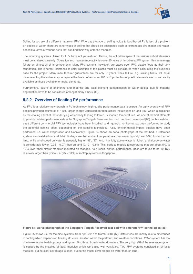
Task 13 Performance, Operation and Reliability of Photovoltaic Systems – Performance of New Photovoltaic System Designs
73
Soiling issues are of a different nature on FPV. Whereas the type of soiling typical to land based PV is less of a problem
on bodies of water, there are other types of soiling that should be anticipated such as extraneous bird matter and water -
based life forms of various sorts that can find their way onto the modules.
The mounting systems utilized for FPV have not yet matured. Hence, the actual life span of the various critical elements
must be analysed carefully. Operation and maintenance activities over 25 years of land-based PV system life can manage
failure on almost all of its components. Many FPV systems, however, are based upon PVC plastic floats as their very
foundation. The inherent resistance to solar radiation of the plastic must be considered when calculating the business
case for the project. Many manufacturer guarantees are for only 10 years. Their failure, e.g. sinking floats, will entail
disassembling the entire array to replace the floats. Aftermarket UV or IR protection of plastic elements are not as readily
available as those available for metal elements.
Furthermore, failure of anchoring and mooring and toxic element contamination of water bodies due to material
degradation have to be considered amongst many others [86].
5.2.2 Overview of floating PV performance
As FPV is a relatively new branch in PV technology, high quality performance data is scarce. An early overview of FPV
designs provided estimates of ~10% larger energy yields compared to similar installations on land [85], which is explained
by the cooling effect of the underlying water body leading to lower PV module temperatures. As one of the first attempts
to provide detailed performance data the Singapore Tengeh Reservoir test-bed has been developed [86]. In this test-bed,
eight different commercial FPV technologies have been installed, and rigorous monitoring has been performed to study
the potential cooling effect depending on the specific technology. Also, environmental impact studies have been
performed, i.e. water evaporation and biodiversity. Figure 54 shows an aerial photograph of the test-bed. A reference
system was installed on land. Main findings are that ambient temperatures over water typically are 2-3°C lower than on
land, while wind speed on water is generally higher [86], [87]. Also, humidity above water is higher, and albedo on water
is considerably lower (0.05 – 0.07) than on land (0.10 – 0.14). This leads to module temperatures that are about 5°C to
10°C lower than similar modules mounted on rooftops. As a result, annual performance ratios are found to be 10-15%
relatively larger than typical PR (75 – 80%) of rooftop systems in Singapore.
Figure 54: Aerial photograph of the Singapore Tengeh Reservoir test-bed with different FPV technologies [88].
Figure 55 shows PR for the nine systems, from April 2017 to March 2018 [87]. Differences are mostly due to differences
in cooling which depends on floating structure, location within the platform, and weather conditions. PR of system A is low
due to excessive bird droppings and system B suffered from inverter downtime. The very high PR of the reference system
is caused by the installed bi-facial modules which were also well ventilated. Two FPV systems consisted of bi-facial
modules, but no clear advantage is seen, due to the much lower albedo on water than on land.

Task 13 Performance, Operation and Reliability of Photovoltaic Systems – Performance of New Photovoltaic System Designs
74
Recent reports on FPV at the west coast of Norway shows similar energy yield advantages of 6 – 10% larger yield for an
FPV system in direct contact with water compared to an comparable air-cooled FPV system [89]. A theoretical study for
an FPV system with horizontally placed modules on the North Sea shows ~4% larger annual PR compared to a land-
based system, where it is noted that this is due to cooling of the modules, and the effect of waves is limited, although
weather and wind patterns have been considered [90]. Another theoretical study shows that energy loss to moving modules
due to waves can range from 3% for medium wave intensity up to 9% for extreme wave intensity [92].
Figure 55: Performance ratio of the FPV systems in the test-bed. Typical PR for rooftop systems in Singapore is
indicated by the blue dashed line, data from [87], [88].
In summary, it can be concluded that FPV systems will show higher energy yields compared to similar systems on land,
but this depends on the type of modules and the specific FPV design. Obviously, more measurements combined with
modelling are needed. Even small-sized experiments can be useful in this respect [93]. Of special interest will be the effect
of (salty) water on long-term reliability.
5.2.3 Examples
Korea Water Resources Corporation 100 kWp and 500 kWp floating PV systems, South Korea
Two research FPV systems have been installed on the Hapcheon dam water reservoir by Korea Water Resources
Corporation starting already in 2011. The 100 kWp system was the first FPV demo system on a dam reservoir in the world.
Both systems are built up using 240 Wp c-Si modules and these are tilted by 33°; actual installed capacity is 99.36 kWp
and 496.8 kWp. The performance has been compared to a 1 MWp land-based PV system on a location 60 km southeast
from Hapcheon, with similar irradiance and temperature. The land-based system comprises 250 Wp modules, tilted by 30°
[80], [85], [94].
Three years of monthly yield data are shown in Figure 56 [94]. The annual yields were 1297, 1364, and 1260 kWh/kWp,
for 2012, 2013, and 2015, respectively. The land-based system showed an annual yield of 1272 kWh/kWp (for 2012),
which would lead to a 2% benefit for the floating system. However, due to missing data, blackouts, maintenance and data
errors, only half of the days in 2012 were useful for comparison. As a conclusion, it was found that the FPV system has
13.5% higher yield than the land-based system, which was attributed to the cooling effect of the water. This has been
found to be more apparent in spring and summer.

Task 13 Performance, Operation and Reliability of Photovoltaic Systems – Performance of New Photovoltaic System Designs
75
Figure 56: Three years of monthly yield data for the 100 kWp FPV system at the Hapcheon dam water reservoir
(data from [94]).
Floating, tracking, cooling, concentrating systems
A special type of FPV systems denoted as Floating, Tracking, Cooling, Concentrating (FTCC) systems have been
developed and deployed in Italy, a 30 kWp pilot system near Pisa and a 200 kWp grid-connected one in Livorno [95]. This
includes reflectors on horizontally placed modules on a platform that is supported by polyethylene tube, and also allows
for efficient vertical one-axis tracking. The system also includes a cooling system for modules, which is reported to increase
energy yield by 15%. The FTCC system performance is reported to be 30% larger than a similar land-based PV system.
A 30 kWp FTCC system was also installed in Cheongju-si, Korea [96].
(a)
(b)
Figure 57: Floating, Tracking, Cooling, Concentrating systems, (a) Colignola-Pisa, Italy [97], (b) Cheongju-si,
Korea [97].
For the performance rating of FPV installation no standards exist. In this section performance factors were proposed, i.e.
the wave intensity, wind speed, or the thermal inertia of the FPV installations. The presented results of the studies differ
significantly regarding the cooling effect of the water body. The measurement protocols are similar but, the measured use
cases differ significantly. The current status is that there is no commonly applicable use case for rating an FPV insta llation´s
performance. Further research activities have to be carried out to find generally valid use cases for FPV performance
characterization. Following a standardization process could be started.

Task 13 Performance, Operation and Reliability of Photovoltaic Systems – Performance of New Photovoltaic System Designs
76
5.3 Performance of agrivoltaics systems: a showcase from Germany
The question of whether to use valuable land for farming or solar power generation has been a subject of fierce debate in
the green energy transition. But the two activities need not be in conflict with each other and, with a new generation of
solar technologies, can in fact be mutually beneficial.
From an economic point of view, generating energy is typically more beneficial for farmers in Germany than producing
food. Thus, about 18% of arable land in Germany is used for growing energy crops. And there is little doubt that Germany
must allocate new land for the production of solar electricity in order to meet the urgent expansion of renewables needed
for the energy transition.
Figure 58: The pilot APV system uses bifacial glass-glass modules arranged in rows of two.
A recent study of Fraunhofer ISE [98] shows that photovoltaic installations in the range of 360 GWp are required in order
to meet the goal of reducing carbon emissions to zero until 2050. This will lead to a significant increase in the competition
for land usage – “food versus fuel” – and at the same time presents an ethical dilemma: valuable, arable land is used to
produce energy, while at the same time food is being imported from threshold and developing countries. As a result, these
countries grow crops for export and less food is available for the indigenous population. But conflicts over land use are
also arising in emerging and developing countries, as growing populations and rising living standards require more energy
and food production.
Instead of being competitors, photovoltaics and photosynthesis can actually complement each other. APV systems make
the efficient dual land usage possible: the farmer not only provides crop yields but also electricity – from the same piece
of land – which dramatically increases the land use efficiency.
Today, numerous APV systems have been installed worldwide. Leading countries in the field are France, Japan, China,
Korea and the United States, with support schemes for APV established. The overall installed capacity is estimated to be
at least 2.4 GWp, with approximately 1.9 GWp in China alone. Nevertheless, only a few research plants exist, and the full
scope of applications is still to be investigated.
5.3.1 Case study Heggelbach: key facts and project structure
In the pilot project “agrophotovoltaics – A Contribution to Resource-Efficient Land Use” (March 2015 to December 2020), technical, social, ecological and economical dimensions of the technology were investigated in a pilot demonstration
project. The seven partners of the model project, led by Fraunhofer ISE and financed by the German Federal Ministry of

Task 13 Performance, Operation and Reliability of Photovoltaic Systems – Performance of New Photovoltaic System Designs
77
Education and Research and FONA (Research for Sustainable Development), also wanted to clarify the political and
energy economical boundary conditions that are required to help the new technology break into the market.
The pilot APV system was installed at the organic Demeter farm in Heggelbach, near Lake Constance. On a test field
covering one third of a hectare, 720 bifacial PV modules with a total power of 194.4 kWp were installed at a vertical
clearance of five meters. This height makes sure that the use of versatile agricultural machinery is not restricted. The rows
of semi-transparent glass-glass modules are placed at a slightly larger distance so that the crops growing underneath
receive at least 60% of the total incoming irradiation. Modules are arranged in rows of two, with a gap between the rows
to better distribute rainwater. The modules’ total surface measures 1206 m2. The deviation from the south is 52°, with a
fixed angle of inclination of 20°.
An important technical aspect was the possibility of deconstructing the plant without, for example, leaving foundations in
the ground. The foundations were therefore laid using a spinning anchor system. In total, about 50 t of steel were used.
One of the Demeter farmers’ demands was that they could carry out their normal crop rotation under the plant: winter
wheat, clover grass, celery and potatoes. The aim for the farmers was to achieve at least 80% of the usual yield. In order
to be able to prove this, the same crops were cultivated on a reference area directly next to the test field.
From September 2016 to June 2019, the solar power and the agricultural yield were assessed.
5.3.2 Microclimatic effects and agricultural yields
Data on the microclimatic parameters such as photosynthetic active radiation (PAR), air and ground temperature as well
as precipitation were collected. The analyses indicated that the PAR under the APV system is reduced by about 30%. In
the first evaluated year, the local air temperatures under the APV system did not differ significantly to the reference plot.
Washouts have been observed at single locations in the field, depending on the crop and its stage of development.
While the clover yield was reduced only slightly (-5.3%) due to shading from the APV, the yield decreases for potatoes (-
18.2%), wheat (-18.7%) and celery (-18.9%) was higher. The winter wheat and the potatoes growing under the PV array
showed a slightly slower development than the same crops on the reference plot. Harvested at the same time, no
mentionable delay in development was observable. The results from the first year of practice showed that all four crops
were qualitatively good and marketable. In comparison to the crops from the reference plot, a lower yield was observed,
but it was still within the target horizon determined in advance by the farmers (80% of reference yield). It has to be noticed
that the harvest was about two weeks too early for some of the plants under the APV array. Normally the potatoes and
celery plants should have been given about two more weeks to ripen. The second year, however, showed a different
picture: In 2018, the yields from three of the four crops grown under the APV system were larger than the reference plot.
The crop yields for celery profited the most by the system, with a gain of 12% compared to the reference. Winter wheat
and potatoes produced a gain of 3 and 11% respectively, and clover a minus of 8%. In addition, in the case of potatoes,
the marketable share (35-50 mm in size) was larger under the APV plant than in the reference area.
In spring and summer, the soil temperature under the APV system was less than on the reference field; while the air
temperature was identical. In the hot, dry summer of 2018, the soil moisture in the wheat crop was higher than on the
reference field, while in the winter months, it was less, as for the other crops. The agricultural scientists of the University
of Hohenheim assume that the shade under the semi-transparent solar modules enabled the plants to better endure the
hot and dry conditions of 2018. In their view, APV could mitigate climate change effects on agriculture in many regions.
For the research project, no particularly shadow-tolerant or even shade-loving plants were selected, but varieties normally
marketed by the Demeter farm. It can be assumed that shade-loving plants such as hops, leafy vegetables, legumes or
certain wine and fruit varieties would have shown significantly better yields. Further follow-up research projects are needed
to investigate this in more detail.
5.3.3 PV performance and electrical storage system
As for the solar yield, the project results of the first year already exceeded expectations, at least with respect to the ini tial
specifications. In the first 12 months of operation, the PV plant produced 245,666 kWh of electricity, or 1,266 kWh/kWp

Task 13 Performance, Operation and Reliability of Photovoltaic Systems – Performance of New Photovoltaic System Designs
78
installed. The power output is mainly influenced by the use of bifacial module technology, but also by a larger distance
from row to row which results in lower shading and temperature losses compared to conventional power plants. A
detrimental factor with regard to the electrical yield is the orientation of the system, which is 52° off south.
In the second year of operation, the solar irradiation totalled 1,319.7 kWh/m², an increase of 8.4% compared to the
previous year. The energy output of the APV system amounted to 249,857 kWh, corresponding to an extraordinarily good
specific yield value of 1285.3 kWh/kWp. Over the day, the power produced by the APV system was well matched to the
power consumption on the Demeter farm. In the summer months, the load demand was covered almost fully by the APV
system and in July close to 100%. The Demeter farmers use it primarily for processing their products and charging their
electrical vehicle. With the subsequent installation of a 150-kWh battery storage system in 2018, the farm community could
increase the own consumption rate for the solar power to approximately 70%. This shows that if the electricity is stored
and used on site, for example for the use of electric agricultural vehicles, additional sources of income arise due to synergy
effects.
While the expected capex costs of an APV plant are about one-third higher than for a conventional open space plant,
mostly due to the higher racking system and higher logistics costs, the operational expenditure costs tend to be about a
quarter lower. This is due to synergy effects such as the avoided costs for mowing, surveillance or a fence. The electricity
production costs of a typical APV system of 2 MWp today are competitive with a small PV rooftop system (<10 kWp).
Further cost reductions due to economies of scale and learning effects are to be expected.
Figure 59: During summer, the APV system covers the electricity load at the farm almost completely. The green
area represents the feed-in of the solar power into the grid, the yellow area represents the own consumption,
while the purchased power from the grid is plotted in grey. Source: BayWa r.e..
5.3.4 Outlook
Now that evidence of increased land use efficiency and economic viability has been provided, to unlock the full potential
of APV, a next step could be further horizontal technology development. To provide the necessary proof-of-concept before
market entry, other techno-economic APV applications should be compared and larger systems in the MW range need to
be realized. E. g. a high potential is expected for APV applications on fruits, berries, hops, and wine.

Task 13 Performance, Operation and Reliability of Photovoltaic Systems – Performance of New Photovoltaic System Designs
79
6 CONCLUSION
With this PVPS Task 13 report, a broad range of methods and protocols for the performance characterization and
performance assessment of new PV system components up to complex new systems with PV is introduced. The report
focuses on new PV components and systems of emerging and growing market segments, where standard characterization
methods and protocols do not exist. The presented methods and protocols may overcome the lack of standardized
performance characterization and assessment methods until such standards are available.
The state of performance characterizations presented in this report can be distinguished into three levels. In the first level,
the introduced performance characterization is related closely to existing standards but provides significant additional
information compared to the standard. In the second level of performance characterization, no standards for the
performance characterization exist. Validated measurement protocols as well as performance indicators are introduced.
Where besides the performance ratio PR, no characterization methods for multiple-usage benefits of the new PV
components and installations are presented operating data of showcases are analysed and discussed to point out possibly
meaningful performance indicators.
Performance characterization level one
For the Multi-MPPT PV inverter, a new test procedure was introduced which enables to rate power losses due to
inhomogeneous load conditions at each MPPT input. The proposed test profiles adjust existing test methods of the current
standard EN 50530 [1] to make PV inverter efficiency a reliable performance indicator also for multi-MPPT PV inverter.
Multi-MPPT PV inverter manufacturers can use this additional information to provide operators and investors with
additional information regarding the efficient operation of their inverters under dynamic inhomogeneous conditions . This
information can be used to calculate the additional economic benefit of multi-MPPT PV inverter and can push technological
multi-MPPT PV inverter development as well as market development.
Performance characterization level two
For the DC/DC optimizers, the performance characterization of a single device can be conducted largely according to
EN 50530 [1] and IEC 62891 [12]. However, it has been pointed out, that the voltage ratio M is not respected in the
standardized characterization methods although it is crucial for meaningful performance figures of DC/DC optimizers with
respect to the possible various operating conditions. Efficiency curves for various voltage ratios M in datasheets would
help in choosing the most efficient PV module – DC/DC inverter combination. Furthermore, the shade mitigation factor
was introduced as an indicator to quantify the additional yield of a DC/DC optimizer equipped PV system by mitigating
shade induced losses compared to a shaded PV reference system. Laboratory tests with a DC/DC optimizer equipped PV
system under dynamic inhomogeneous shading conditions showed higher energy yields than a standard PV system with
string inverter but considerably less than the often claimed two-digit number percentage. The report provides methods and
measurement protocols for rating DC/DC optimizers´ performance and enables the market to design PV systems with
DC/DC optimizer more precisely and to quantify and rate their yield benefit for specific applications.
PV AC modules where PV module and microinverter are fully integrated have to be characterized as a whole, so
established standards as IEC 61853 [18] and EN 50530 [1] for the individual characterization of a PV module and a (micro-
) inverter are not applicable. The report presents a validated method comprising a measurement protocol and a simulation
model for PV AC modules. It enables the market players to conduct simulations for individual PV AC module use cases
and make them comparable to other PV-module-inverter combinations.
With the section of shade resilient PV module designs, the report provides information about the possible shade loss
mitigation increasing the PV module granularity or even the PV cell granularity for PV modules under highly dynamic
inhomogeneous operating conditions. The presented results show for which application cases the investigated granular
PV module or PV cell concepts can gain valuable benefit.
With the presented “Efficiency guideline for PV storage systems” published by the German Energy Storage Association BVES and German Solar Industry Association BSW, manufacturers have a well-defined measurement protocol (not yet a
Task 13 Performance, Operation and Reliability of Photovoltaic Systems – Performance of New Photovoltaic System Designs
80
standard) at hand to provide the market with reliable and comparable performance figures of their battery storage products.
The presented showcase using the efficiency guideline´s measurement protocol, the PV battery storage simulation model
and the concise cycle test makes performance characterization of PV battery storages in individual dynamic building
energy systems with limited effort possible and comparable. Even in Germany, where in 2019 about 90 % of new private
PV installations were equipped with a battery storage, the validated measurement protocols and methods, validated
simulation models as well as new meaningful performance indicators, introduced and discussed in the report, can enhance
the confidence in PV battery storages. This can lead to increasing the share of PV installations with battery storage,
creating additional value and enhancing the energy transition where energy storage capacities are urgently needed.
Performance characterization level three
The performance characterization of agricultural PV systems (APV) is between level two and three of performance
characterization. With the land equivalent ratio LER, one performance indicator exists besides the performance ratio PR.
Nonetheless, more performance indicators such as the marketable crop size were proposed and evaluated for the
introduced showcase. The showcase results in agricultural and energy yield pointed out that the combination of cultivated
crops, weather and climate conditions on site and the specific PV system design have to be investigated as a whole to
gain the most benefit of agricultural PV systems. With this information, the report gives the market valuable information at
hand for further development of the APV sector, while scarcity of free areas for large PV generators and climate change
with water shortage forces farmers to adapt their cultivation methods.
The performance of showcases of net integrated PV system with battery storage is assigned to level three of performance
characterization. For these off-grid systems the PR does work as a performance indicator only when the produced PV
energy is not curtailed. Under PV curtailment the number of battery system charging and discharging cycles, the number
of generator uptakes when batteries are exhausted, the number of days with a battery state of charge below a certain limit
and the number exceeding of power quality boundaries were proposed as performance indicators. By rating real operation
data or system simulation results with the proposed performance indicators, system designers and operators are enabled
to optimize their systems in terms of efficiency, reliability and maintenance efforts to improve their systems´
competitiveness and increase their market share.
Floating PV systems are an upcoming market with increasing growth, although further research on their performance
characterization methods and performance indicators besides the PR is necessary. The introduced floating PV
performance characterization methods and indicators can be assigned to level three as several indicators and
measurement protocols in showcases have shown, but no uniform approach for rating floating PV systems is established
or standardized yet. E. g. measurement protocols with comparative operation of floating PV systems and land-based
reference systems to quantify yield differences and qualify the reason for them were introduced. That may give market
players valuable advice which environmental conditions have to be considered most, to speed up the development of
floating PV market.
This report as a compendium of performance characterization of new PV components and complex systems with PV
shows that the performance characterization and the performance characterization indicators are as manifold as the
additional benefits of the assessed systems are. To develop a uniform performance indicator for all kinds of new PV
components or new complex systems with PV will hardly be possible. However, a frame work should be developed which
allows the normalization of different performance indicators in order to make them comparable.
Task 13 Performance, Operation and Reliability of Photovoltaic Systems – Performance of New Photovoltaic System Designs
81
REFERENCES
[1] “DIN EN 50530 (VDE 0126-12:2013-12):2013-12, Gesamtwirkungsgrad von Photovoltaik-Wechselrichtern; Deutsche Fassung EN 50530:2010 + A1:2013.” Berlin, 2013.
[2] “IEC: „Photovoltaic systems - Power conditioners - Procedure for measuring efficiency“, IEC 61683 ed.1 (1999-11).” 1999.
[3] “IEC 61724 Photovoltaic System Performance Monitoring—Guidelines for Measurement, Data Exchange and Analysis, 10th ed.” Geneva, Switzerland, 1998.
[4] D. Gfeller, U. Muntwyler, and L. Borgna, “Testing of multi-MPPT PV inverters: approach and test results,” 32nd European Photovoltaic Solar Energy Conference and Exhibition. Munich, Germany, pp. 2138–2143, 2016.
[5] “IEC 60904-1:2006 Photovoltaic devices - Part 1: Measurement of photovoltaic current-voltage characteristics.” 2006.
[6] S. M. MacAlpine, R. W. Erickson, and M. J. Brandemuehl, “Characterization of power optimizer potential to increase energy capture in photovoltaic systems operating under nonuniform conditions,” IEEE Transactions on Power Electronics, vol. 28, no. 6. pp. 2936–2945, 2013.
[7] G. Ball and J. Fisher, “Rooftop PV Systems and Firefighter Safety, Proceedings,” 2016 IEEE 43rd Photovoltaic Specialists Conference (PVSC 2016). Portland, Oregon, USA, pp. 1244–1250, 2016.
[8] Q. Gao, Y. Zhang, Y. Yu, and Z. Liu, “A direct current-voltage measurement method for smart photovoltaic modules with submodule level power optimizers,” Solar Energy, vol. 167. pp. 52–60, 2018.
[9] Perry Tsao, Sameh Sarhan, and Ismail Jorio, “Distributed max power point tracking for photovoltaic arrays,” 2009 34th IEEE Photovoltaic Specialists Conference (PVSC). pp. 2293–2298, 2009.
[10] C. A. Deline, “Deline unpublished.” . [11] “ASTM E1036 - 15(2019) Standard Test Methods for Electrical Performance of
Nonconcentrator Terrestrial Photovoltaic Modules and Arrays Using Reference Cells.” West Conshohocken, PA, 2019.
[12] “IEC 62891:2015-05 Overall efficiency of grid connected photovoltaic inverters.” 2015.
[13] C. Deline and S. Macalpine, “Use conditions and efficiency measurements of DC power optimizers for photovoltaic systems,” 2013 IEEE Energy Conversion Congress and Exposition, ECCE 2013, no. October. pp. 4801–4807, 2013.
[14] C. Deline, J. Meydbray, and M. Donovan, “Photovoltaic Shading Testbed for Module-level Power Electronics: 2016 Performance Data Update,” no. NREL Technical Report NREL/TP-5J00-62471. 2016.

Task 13 Performance, Operation and Reliability of Photovoltaic Systems – Performance of New Photovoltaic System Designs
82
[15] C. Deline, B. Sekulic, J. Stein, S. Barkaszi, J. Yang, and S. Kahn, “Evaluation of Maxim module-Integrated electronics at the DOE Regional Test Centers,” 2014 IEEE 40th Photovoltaic Specialist Conference, PVSC 2014, no. June. pp. 986–991, 2014.
[16] Solar Edge, “SolarEdge Efficiency of P Series Power Optimizers,” 2018. [17] A. J. Hanson, C. A. Deline, S. M. MacAlpine, J. T. Stauth, and C. R. Sullivan,
“Partial-Shading Assessment of Photovoltaic Installations via Module-Level Monitoring,” IEEE Journal of Photovoltaics, vol. 4, no. 6. pp. 1618–1624, Nov-2014.
[18] “IEC 61853-1:2011 Photovoltaic (PV) module performance testing and energy rating - Part 1: Irradiance and temperature performance measurements and power rating.” Berlin, 2011.
[19] D. M. Riley, C. W. Hansen, and M. Farr, “A Performance Model for Photovoltaic Modules with Integrated Microinverters,” no. January. Albuquerque, New Mexico, p. 55, 2015.
[20] C. Allenspach, V. Castro de Echavarri, S. Richter, C. Meier, F. Carigiet, and F. Baumgartner, “MODULE-LEVEL POWER ELECTRONICS UNDER INDOOR PERFORMANCE TESTS Scope / Objectives,” 37th European Photovoltaic Solar Energy Conference (EUPVSEC). Lisbonb, Portugal, 2020.
[21] F. P. Baumgartner, “Euro Realo inverter efficiency: DC-voltage dependency,” 20th European Photovoltaic Solar Energy Conference and Exhibition, no. June. p. 2257, 2005.
[22] F. Baumgartner, “Photovoltaic (PV) balance of system components,” The Performance of Photovoltaic (PV) Systems. Elsevier, pp. 135–181, 2017.
[23] P. Moraitis, B. B. Kausika, N. Nortier, and W. Van Sark, “Urban environment and solar PV performance: The case of the Netherlands,” Energies, vol. 11, no. 6. 2018.
[24] K. Sinapis, T. T. H. Rooijakkers, L. H. Slooff, L. A. G. Okel, M. J. Jansen, and A. J. L. Carr, “Towards new module and system concepts for linear shading response.” 2017.
[25] S. Silvestre, A. Boronat, and A. Chouder, “Study of bypass diodes configuration on PV modules,” Applied Energy, vol. 86, no. 9. pp. 1632–1640, 2009.
[26] K. Sinapis et al., “Annual Yield Comparison of Module Level Power Electronics and String Level PV Systems with Standard and Advanced Module Design,” 32nd European Photovoltaic Solar Energy Conference and Exhibition. Munich, Germany, pp. 2011–2015, 2016.
[27] B. B. Pannebakker, A. C. de Waal, and W. G. J. H. M. van Sark, “Photovoltaics in the shade: one bypass diode per solar cell revisited,” Progress in Photovoltaics: Research and Applications, vol. 25, no. 10. pp. 836–849, 2017.
[28] K. Sinapis, T. T. H. Rooijakkers, and W. G. J. H. M. van Sark, “Effects of solar cell group granularity and modern system architectures on partial shading response of c-Si modules and systems,” IEEE Journal of Photovoltaics, vol.
Task 13 Performance, Operation and Reliability of Photovoltaic Systems – Performance of New Photovoltaic System Designs
83
submitted. 2020.
[29] K. Sinapis et al., “A comprehensive study on partial shading response of c-Si modules and yield modeling of string inverter and module level power electronics,” Solar Energy, vol. 135. pp. 731–741, 2016.
[30] S. K. Das, D. Verma, S. Nema, and R. K. Nema, “Shading mitigation techniques: State-of-the-art in photovoltaic applications,” Renewable and Sustainable Energy Reviews, vol. 78. pp. 369–390, 2017.
[31] D. Nguyen and B. Lehman, “An Adaptive Solar Photovoltaic Array Using Model-Based Reconfiguration Algorithm,” IEEE Transactions on Industrial Electronics, vol. 55, no. 7. pp. 2644–2654, 2008.
[32] G. Velasco-Quesada, F. Guinjoan-Gispert, R. Pique-Lopez, M. Roman-Lumbreras, and A. Conesa-Roca, “Electrical PV Array Reconfiguration Strategy for Energy Extraction Improvement in Grid-Connected PV Systems,” IEEE Transactions on Industrial Electronics, vol. 56, no. 11. pp. 4319–4331, Nov-2009.
[33] A. Bidram, A. Davoudi, and R. S. Balog, “Control and Circuit Techniques to Mitigate Partial Shading Effects in Photovoltaic Arrays,” IEEE Journal of Photovoltaics, vol. 2, no. 4. pp. 532–546, 2012.
[34] S. Z. M. Golroodbari, A. C. De Waal, and W. G. J. H. M. Van Sark, “Improvement of shade resilience in photovoltaic modules using buck converters in a smart module architecture,” Energies, vol. 11, no. 1. 2018.
[35] B. Burger, B. Goeldi, S. Rogalla, and H. Schmidt, “25th European Photovoltaic Solar Energy Conference and Exhibition / 5th World Conference on Photovoltaic Energy Conversion, 6-10 September 2010, Valencia, Spain,” 25th European Photovoltaic Solar Energy Conference and Exhibition, no. September. Valencia, Spain, pp. 3700–3707, 2010.
[36] C. Olalla, D. Clement, M. Rodriguez, and D. Maksimovic, “Architectures and Control of Submodule Integrated DC–DC Converters for Photovoltaic Applications,” IEEE Transactions on Power Electronics, vol. 28, no. 6. pp. 2980–2997, 2013.
[37] M. Uno and A. Kukita, “Current Sensorless Equalization Strategy for a Single-Switch Voltage Equalizer Using Multistacked Buck–Boost Converters for Photovoltaic Modules Under Partial Shading,” IEEE Transactions on Industry Applications, vol. 53, no. 1. pp. 420–429, Jan-2017.
[38] S. Z. M. Golroodbari, A. C. De Waal, and W. G. J. H. M. Van Sark, “Proof of concept for a novel and smart shade resilient photovoltaic module,” IET Renewable Power Generation, vol. 13, no. 12. pp. 2184–2194, 2019.
[39] A. J. Carr, M. J. Jansen, M. de Bruijne, L. Okel, M. Kloos, and W. Eerenstein, “High voltage MWT module with improved shadow performance,” 2014 IEEE 40th Photovoltaic Specialist Conference (PVSC). pp. 2685–2688, 2014.
[40] A. J. Carr et al., “Tessera: Scalable, shade robust module,” 2015 IEEE 42nd Photovoltaic Specialist Conference (PVSC). pp. 1–5, 2015.

Task 13 Performance, Operation and Reliability of Photovoltaic Systems – Performance of New Photovoltaic System Designs
84
[41] L. H. Slooff et al., “Shade response of a full size TESSERA module,” Japanese Journal of Applied Physics, vol. 56, no. 8S2. IOP Publishing, p. 08MD01, Jul-2017.
[42] K. Sinapis, R. Pacheco Bubi, L. H. Slooff, W. Folkerts, L. A. G. Okel, and M. J. Jansen, “Outdoor performance characterization of a novel shadow tolerant module,” 35th European Photovoltaic Solar Energy Conference (EUPVSEC). Brussels, Belgium, pp. 1169–1171, 2018.
[43] German Energy Storage Association (BVES) and German Solar Industry Association (BSW), “Efficiency guideline for PV storage systems.” Berlin, Germany, 2019.
[44] C. Allenspach, R. Koch, E. Kinigadner, F. Carigiet, and F. Baumgartner, “Solarbatteriesystem und transienter ‘NESPRESS-Test’ in der ZHAW Bachelorausbildung,” österreichischen Fachtagung für Photovoltaik & Stromspeicherung. Vienna, Austria, 2019.
[45] M. Knoop and M. Littwin, “MATLAB-basiertes Simulationsmodell zur Berechnung der elektrischen Leistungsflüsse im PV-Speichersystem,” 32. Symposium Photovoltaische Solarenergie. OTTI e.V., Bad Staffelstein, Germany, 2017.
[46] D. Linden and T. B. Reddy, “Handbook of Batteries, third edition,” McGraw-Hill. 2002.
[47] M. Littwin and M. Kesting, “Experimentalanlage zur Untersuchung interaktiver Strom- und Wärmeversorgungssysteme in Gebäuden Universelle und flexible Untersuchungsmöglichkeiten mit der Experimentalanlage für integrierte Gesamtenergiesysteme,” 30. Symposium Photovoltaische Solarenergie. 2015.
[48] J. Kalisch and et al, “Continuous meteorological observations in high-resolution (1Hz) at University of Oldenburg in 2014.” Carl-von-Ossietzky University of Oldenburg, Oldenburg, 2015.
[49] Bundesverband der Energie- und Wasserwirtschaft e.V, “Energie-Info: Stromverbrauch im Haushalt.” Berlin, p. 34, 2013.
[50] Hochschule für Technik und Wirtschaft HTW Berlin, “Repräsentative elektrische Lastprofile für Einfamilienhäuser in Deutschland auf 1-sekündiger Datenbasis.” Berlin, 2015.
[51] P. Vogelsanger, “The Concise Cycle Test Method - a Twelve Day System Test,” A Report of IEA SHC - Task 26 Solar Combisystems A technical report of Subtask B, no. November. 2002.
[52] R. Haberl, A. Reber, E. Bamberger, and M. Haller, “Hardware-in-the-Loop Tests on Complete Systems with Heat Pumps and PV for the Supply of Heat and Electricity.” 2018.
[53] “IEC 61427-2:2015 Secondary cells and batteries for renewable energy storage - General requirements and methods of test - Part 2: On-grid applications.” p. 108, 2015.
[54] “IEC 62933-2-1:2017 Electric energy storage (EES) systems - Part 2-1: Unit

Task 13 Performance, Operation and Reliability of Photovoltaic Systems – Performance of New Photovoltaic System Designs
85
parameters and testing methods - General specifications Edition 1.0.” p. 85, 2017.
[55] J. Weniger, S. Maier, N. Orth, and V. Quaschning, “Energy Storage Inspection 2020 (English summary).” Berlin, Germany, 2020.
[56] J. Weniger, N. Orth, N. Böhme, and V. Quaschning Forschungsgruppe Solarspeichersysteme, “Stromspeicher-Inspektion 2Q19 (Präsentation deutsch).” Berlin, Germany, 2019.
[57] “Testbench Testverfahren zur Bestimmung der Effizienz von PV-Speichersystemen – Vom Leitfaden zum Standard.” 2020.
[58] C. Dupraz, H. Marrou, G. Talbot, L. Dufour, A. Nogier, and Y. Ferard, “Combining solar photovoltaic panels and food crops for optimising land use: Towards new agrivoltaic schemes,” Renewable Energy, vol. 36, no. 10. pp. 2725–2732, 2011.
[59] A. GOETZBERGER and A. ZASTROW, “On the Coexistence of Solar-Energy Conversion and Plant Cultivation,” International Journal of Solar Energy, vol. 1, no. 1. Taylor & Francis, pp. 55–69, 1982.
[60] R. Mead and R. W. Willey, “The Concept of a ‘Land Equivalent Ratio’ and Advantages in Yields from Intercropping,” Experimental Agriculture, vol. 16, no. 3. Cambridge University Press, pp. 217–228, 03-Jul-1980.
[61] H. Marrou, L. Guilioni, L. Dufour, C. Dupraz, and J. Wery, “Microclimate under agrivoltaic systems: Is crop growth rate affected in the partial shade of solar panels?,” Agricultural and Forest Meteorology, vol. 177. Elsevier B.V., pp. 117–132, 15-Aug-2013.
[62] R. W. Willey, “Evaluation and Presentation of Intercropping Advantages,” Experimental Agriculture, vol. 21, no. 2. Cambridge University Press, pp. 119–133, 1985.
[63] B. Müller, L. Hardt, A. Armbruster, K. Kiefer, and C. Reise, “Yield predictions for photovoltaic power plants: empirical validation, recent advances and remaining uncertainties,” Progress in Photovoltaics: Research and Applications, vol. 24, no. 4. pp. 570–583, 2016.
[64] D. Majumdar and M. J. Pasqualetti, “Dual use of agricultural land: Introducing ‘agrivoltaics’ in Phoenix Metropolitan Statistical Area, USA,” Landscape and Urban Planning, vol. 170. pp. 150–168, 2018.
[65] J. Weaver, “Agrovoltaics: a solar-powered safety net for Massachusetts farmers – pv magazine USA,” pv magazine USA. Aug-2018.
[66] J. Movellan, “Japan Next-Generation Farmers Cultivate Crops and Solar Energy - Renewable Energy World.” 08-Oct-2013.
[67] A. Bluechel and F. Baumgartner, “SOLAR SYSTEM WITH CLEANING DEVICE WO20141798934 (A1) und WO2014179893 (A1) ― 2014-11-13.” p. 26, 2014.
[68] F. Baumgartner et al., “‘Urban Plant’ Light-Weight Solar System for Parking and other Urban Double Use Applications,” 28th European Photovoltaic Solar Energy Conference and Exhibition. Paris, France, pp. 2897–2901, 2013.

Task 13 Performance, Operation and Reliability of Photovoltaic Systems – Performance of New Photovoltaic System Designs
86
[69] G. A. Diem and A. Hügli, “Operating data fom a 640 kW HORIZON solar foldable PV plant on top of the wastewater retreatment basins in Chur, Switzerland.” Zizers, Switzerland, 2019.
[70] A. Sahu, N. Yadav, and K. Sudhakar, “Floating photovoltaic power plant: A review,” Renewable and Sustainable Energy Reviews, vol. 66. pp. 815–824, 2016.
[71] R. Cazzaniga, M. Cicu, M. Rosa-Clot, P. Rosa-Clot, G. M. Tina, and C. Ventura, “Floating photovoltaic plants: Performance analysis and design solutions,” Renewable and Sustainable Energy Reviews, vol. 81. pp. 1730–1741, 2018.
[72] P. Ranjbaran, H. Yousefi, G. B. Gharehpetian, and F. R. Astaraei, “A review on floating photovoltaic (FPV) power generation units,” Renewable and Sustainable Energy Reviews, vol. 110. pp. 332–347, 2019.
[73] K. Trapani and D. L. Millar, “Proposing offshore photovoltaic (PV) technology to the energy mix of the Maltese islands,” Energy Conversion and Management, vol. 67, no. March. pp. 18–26, 2013.
[74] I. Kougias et al., “The potential of water infrastructure to accommodate solar PV systems in Mediterranean islands,” Solar Energy, vol. 136. Elsevier Ltd, pp. 174–182, 15-Oct-2016.
[75] M. Rosa-Clot and G. M. Tina, Eds., “Floating PV Plants.” Academic Press, p. 138, 2020.
[76] M. Rosa-Clot and G. M. Tina, “Submerged and Floating Photovoltaic Systems Modelling, Design and Case Studies.” Academic Press, p. 262, 2017.
[77] J. Haas, J. Khalighi, A. De La Fuente, S. U. Gerbersdorf, W. Nowak, and P.-J. Chen, “Floating photovoltaic plants: Ecological impacts versus hydropower operation flexibility.” 2019.
[78] R. Cazzaniga, M. Rosa-Clot, P. Rosa-Clot, and G. M. Tina, “Integration of PV floating with hydroelectric power plants,” Heliyon, vol. 5, no. 6. Elsevier Ltd, 01-Jun-2019.
[79] World Bank Group, ESMAP, and SERIS, “Where Sun Meets Water FLOATING SOLAR HANDBOOK FOR PRACTITIONERS.” Washington, DC, p. 155, 2019.
[80] Y.-K. Choi, “A Study on Power Generation Analysis of Floating PV System Considering Environmental Impact,” International Journal of Software Engineering and Its Applications, vol. 8, no. 1. pp. 75–84, 2014.
[81] Z. Wang, R. Carriveau, D. S.-K. Ting, W. Xiong, and Z. Wang, “A review of marine renewable energy storage,” International Journal of Energy Research, vol. 43, no. 12. pp. 6108–6150, 2019.
[82] A. M. Pringle, R. M. Handler, and J. M. Pearce, “Aquavoltaics: Synergies for dual use of water area for solar photovoltaic electricity generation and aquaculture,” Renewable and Sustainable Energy Reviews, vol. 80. pp. 572–584, 2017.
[83] K. Trapani and D. L. Millar, “The thin film flexible floating PV (T3F-PV) array: The concept and development of the prototype,” Renewable Energy, vol. 71. pp. 43–

Task 13 Performance, Operation and Reliability of Photovoltaic Systems – Performance of New Photovoltaic System Designs
87
50, 2014.
[84] K. Trapani, “No TitleFlexible floating thin film photovoltaic (PV) array concept for marine and lacustrine environments.” pp. 1–217, 2014.
[85] K. Trapani and M. Redón Santafé, “A review of floating photovoltaic installations: 2007–2013,” Progress in Photovoltaics: Research and Applications, vol. 23, no. 4. pp. 524–532, 2015.
[86] H. Liu, V. Krishna, J. Lun Leung, T. Reindl, and L. Zhao, “Field experience and performance analysis of floating PV technologies in the tropics,” Progress in Photovoltaics: Research and Applications, vol. 26, no. 12. pp. 957–967, 2018.
[87] T. Reindl, “World’s largest Floating Solar Testbed - Overview and Findings,” ACEF Deep Dive Workshop on Floating Solar. Singapore, 2018.
[88] T. Reindl, “At the heart of floating solar: Singapore,” PV Tech Power, vol. 14, no. Buoyant Market. pp. 18–23, 2018.
[89] J. H. Selj et al., “THE PERFORMANCE OF A FLOATING PV PLANT AT THE WEST COAST OF NORWAY,” 36th European Photovoltaic Solar Energy Conference and Exhibition, vol. 46, no. 3. Marseilles, France, pp. 1763–1767, 2019.
[90] S. Z. Golroodbari and W. Van Sark, “Simulation of performance differences between offshore and land-based photovoltaic systems,” Progress in Photovoltaics, vol. 28, no. 9. pp. 873–886, 2020.
[91] S. Z. Golroodbari and W. van Sark, “Simulation of performance differences between offshore and land-based photovoltaic systems,” Progress in Photovoltaics: Research and Applications, vol. n/a, no. n/a. .
[92] M. Dörenkämper, D. van der Werf, K. Sinapis, M. M. de Jong, and W. Folkerts, “INFLUENCE OF WAVE INDUCED MOVEMENTS ON THE PERFORMANCE OF FLOATING PV SYSTEMS,” 36th European Photovoltaic Solar Energy Conference and Exhibition. Marseiles, France, pp. 1759–1762, 2019.
[93] M. Kumar and A. Kumar, “Experimental characterization of the performance of different photovoltaic technologies on water bodies,” Progress in Photovoltaics. p. 24, 2019.
[94] J. Suh, Y. Jang, and Y. Choi, “Comparison of electric power output observed and estimated from floating photovoltaic systems: A case study on the hapcheon dam, Korea,” Sustainability, vol. 12, no. 1. p. 14, 2020.
[95] R. Cazzaniga, M. Rosa-Clot, P. Rosa-Clot, and G. M. Tina, “Floating tracking cooling concentrating (FTCC) systems,” 2012 38th IEEE Photovoltaic Specialists Conference. pp. 514–519, 2012.
[96] S. H. Kim, S. J. Yoon, W. Choi, and K. B. Choi, “Application of floating photovoltaic energy generation systems in South Korea,” Sustainability, vol. 8, no. 12. pp. 1–9, 2016.
[97] Koiné Multimedia, “Floating Tracking Cooling Concentrator.” [Online]. Available: http://www.koinemultimedia.eu/wp/sample-page/. [Accessed: 06-Oct-2020].

Task 13 Performance, Operation and Reliability of Photovoltaic Systems – Performance of New Photovoltaic System Designs
88
[98] P. Sterchele et al., “WEGE ZU EINEM KLIMANEUTRALEN ENERGIESYSTEM Die deutsche Energiewende im Kontext gesellschaftlicher Verhaltensweisen.” Freiburg i.B., p. 66, 2020.

Task 13 Performance, Operation and Reliability of Photovoltaic Systems – Performance of New Photovoltaic System Designs
89
![[Architecture Ebook] Building-integrated Photovoltaic Designs for Commercial and Industrial Structures](https://img.pdfslide.net/doc/110x75/577d2f1d1a28ab4e1eb0d63f/architecture-ebook-building-integrated-photovoltaic-designs-for-commercial.jpg)