136

CHAPTER 7

PERFORMANCES OF MICROSTRIP FRACTAL ANTENNA WITH WATER

LAYERS

7.1 INTRODUCTION

Modern telecommunication system requires antennas that have multiband and wider

bandwidth characteristics as well as smaller dimensions than conventionally possible. This

demand has initiated antenna research in various directions, one of which is fractal

geometry shaped antennas. As well known there is an important relation between antenna

dimensions and wavelength, which states if antenna size is less than λ/4 (λ is wave length)

the antenna will not be an efficient radiator because radiation resistance, gain and

bandwidth is very much reduced. Fractal geometry is a very good solution for this problem.

Fractals are geometric shapes, which are self similar; repeating themselves at different

scales. Hence these structures are recognized by their self similarity properties and

fractional dimension as whole.

In the recent years, the geometrical properties of self-similar and space filling nature has

motivated antenna design engineers to adopt this geometry as viable alternative to meet the

target of multiband operation. Fractional dimensions, self-similar and scaling properties,

characterize these structures. The structures that are studied as antenna are not the ones that

we obtained after infinite iteration but those after finite iterations as desired by the

designer. The space filling property lead to curves that is electrically very long but fit into a

compact physical space. This property can lead to the miniaturization of antennas. With the

development of fractal theory, the nature of fractal geometries in antenna design has led to

the evolution of a new class of antennas, called fractal shaped antennas. Fractal geometries

in the antenna application are becoming major concern for many researchers these days.

Due to the fractal configuration large electrical length is fitted into the small physical

volume. Thus the high convoluted shape of a fractal allows reducing the overall volume

occupied by the resonating element. As we know, mobile communications has become an

137

important part of the human life. Mobile means practical for user and easily transportable.

Thus the mobile terminals for wireless application should be light, small and should have

low energy consumption to satisfy these requirements. Due to greater integration of

electronics, the size of transceiver needed for the mobile applications have decreased

drastically. Hence the size of the antenna should be compatible with the dimensions of the

receiver or the repeater system, especially at the lower microwave spectrum.

Fractals mean broken or irregular fragments. Fractals describe a complex set of geometries

ranging from self similar/ self-affine to other irregular structure. Fractals are generally

composed of multiple copies of themselves at different scales and hence do not have a

predefined size which makes their use in antenna design very promising. Fractal antenna

engineering is an emerging field that employs fractal concepts for developing new types of

antennas with notable characteristics. Fractal shaped antennas show some interesting

features which results from their geometrical properties. The unique features of fractals

such as self-similarity and space filling properties enable the realization of antennas with

interesting characteristics such as multi-band operation and miniaturization. A self-similar

set is one that consists of scaled down copies of itself. This property of self-similarity of

the fractal geometry aids in the design of fractal antennas with multiband characteristics.

The self-similar current distribution on these antennas is expected to cause its multiband

characteristics.

The space-filling property of fractals tends to fill the area occupied by the antenna as the

order of iteration is increased.Higher order fractal antennas exploit the space-filling

property and enable miniaturization of antennas. Fractal antennas and arrays also exhibit

lower side-lobe levels.

Koch fractal geometry was originally introduced by a Helge von Koch in 1904. One starts

with a straight line, called the initiator. This is partitioned into three equal parts, and the

segment at the middle is replaced with two others of the same length. This is the first

iterated version of the geometry and is called the generator. The process is reused in the

generation of higher iterations. The number of iterations defines the order of the fractals.

7.2. RECENT DEVELOPMENTS IN FRACTAL PATCH ANTENNA

138

In 1998, Z. Baharav presented his work on fractal arrays based in iterated functions system.

Self similar feature in the radiation patterns will allow a multi-band frequency usage of the

fractal array [1]. Most of the previous works done in this area deals with fractal arrays in

which the distance between the elements is some fractal function (like the Cantor set),

whereas their amplitude is constant. This work, on the other hand, deals with uniformly

spaced elements, whereas the elements amplitude distribution is a fractal function. In this

work we will use the Iterated Function System (IFS) method to produce fractals. It can lead

to an automated method for fractal encoding of signals. The use of the IFS will enable one

to create fractal arrays with many degrees of freedom.

In 1999, M. Navarro et al. worked on the topic ―Self-Similar surface current distribution

on fractal Sierpinski Antenna verified with Infra-red Thermograms‖ [2]. In this research he

presented the experimental verification of the fractal Sierpinski Antenna Surface current

distribution. Measures data from an infrared camera agree with a numerical data showing a

self -similar behavior in the current density distribution over the fractal antenna surface.

The obtained results gave a better insight on the multiband behavior of the fractal-shape

antenna.

In 2001, P. Felber et al. had done some research on fractal antennas [3]. In this research he

limited his study only to fractal antenna elements and fractal arrays. Traditional wideband

antennas (spiral and log-periodic) and arrays can be analyzed with fractal geometry to shed

new light on their operating principles. More to the point, a number of new configurations

can be used as antenna elements with good multiband characteristics. Due to the space

filling properties of fractals, antennas designed from certain fractal shapes can have far

better electrical to physical size ratios than antennas designed from an understanding of

shapes in Euclidean space. In 2004, K. Sathya et al. performed research on size reduction

of low frequency microstrip patch antenna with Koch shaped fractal slot. In this, a

microstrip patch antenna with Koch shaped fractal slot implemented with a foam substrate

= 1.02 was shown to bring a size reduction of about 84% compared to an ordinary

microstrip patch antenna for the same resonant frequency [4]. A compromised design of a

two element array pattern of the single structure gives considerable gain as well as 66%

size reduction. In 2005, P. Hazadra et al. performed the research on model analysis of

fractal microstrip patch antennas [5]. The full wave simulation of complex structure is very

139

difficult and time consuming that is why cavity model has been found which is very useful

in obtaining basic parameters of structures like resonant frequencies, field distribution and

radiation pattern. The results obtained are in good agreement with the full wave simulation

performed by IE3D simulator.

Later in 2006, N. Gupta performed the research on ―Two compact microstrip patch antenna

for 2.4 GHz band‖. In this two low profile patch antenna for wireless LAN 802.11b

communication standard was proposed and investigated [6]. The proposed patch antenna

shows a significant size reduction compared to the simple square patch antenna, the gain

and bandwidth of the proposed antennas found to be increased significantly using stacked

configuration. In 2007, V. R. Gupta et al. performed analysis on fractal microstrip patch

antenna [7]. In this research they studied the effect of increase in electrical length at each

iterative step in the generation of the fractal. Although there are number of methods to

reduce the size of the antenna operating at the lower frequencies and fractal is one among

them. In this research it was found that Fractal patch antenna are good candidates for size

reduction as large electrical length can be fitted into the small physical volume. However to

make the antenna resonate at a particular frequency the useful range of size reduction lies

only up to third iteration. In 2008, F.H. Kashani at el. performed the research on a novel

broadband fractal sierpinski shaped, microstrip antenna. In this research new microstrip

Sierpinski modified and fractalized antenna using multilayer structure for achieving wide

band behavior in X- band which in 7-10.6 GHz portion overlaps UWB working range [8].

Working range for this antenna is from 7.7 GHz to 16.7 GHz (bandwidth = 9 GHz). In this,

a new small microstrip antenna for ultra wideband application was designed and modified.

However in 2009, A. Azari et al. performed the research on ultra wide band fractal

microstrip antenna design. In this research he presented new fractal geometry for microstrip

antennas. In this research a new hexagonal fractal was presented [9]. This fractal antenna

has a very high bandwidth; multiband in nature and good properties as well as significant

gain improvement was achieved. In 2010, Fawwaz J. Jibrael at el. performed the research

on ―A new multiband patch microstrip plusses fractal antenna‖.

The proposed antenna has shown to possess an excellent size reduction possibility with

good radiation performance for wireless applications [10].

140

Therefore, it is being observed that no research works have done on dielectric loaded

fractal patch antennas, though loading severely affects the performances of the patch

antennas, hence attention have paid to describe the effects of dielectric loading on its

operating performances. Figure 7.1 shows the proposed fractal geometry of patch antenna

designed for the pentagonal fractal patch antenna up to third iteration. The proposed

antenna has shown four resonant bands at frequency of 2.471 GHz , 7.032 GHz, 8.651

GHz, and 11.86 GHz, and at these frequencies the antenna has S11 < - 10 dB (VSWR < 2).

Hence it can be used as a multiband antenna in wireless applications successfully.

Figure 7.1 Proposed fractal geometries of pentagonal patch antenna

7.3. DESIGN SPECIFICATIONS

Design parameters for pentagonal patch antenna are given below.

Third Iteration

First Iteration

Second Iteration

Zero Iteration

141

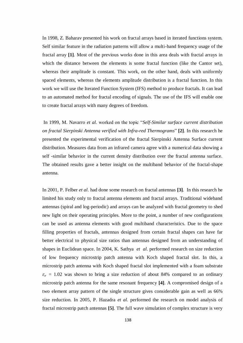
Geometry Pentagonal

Side arm length 28.52 mm

Substrate (FR-4) εr = 4.4, h = 0.8mm, tanδ = 0.02

Centre frequency 2.45 GHz

Feed location(From Center) 8.21 mm

Coaxial cable dimension Inner radius: 0.5 mm

Outer radius:0.9 mm

Dielectric cover (Distilled water) εr=81, h=0.1mm to 0.3 mm

Side arm length of the pentagonal 28.52 mm

7.4. ANTENNA GEOMETRY AND CONFIGURATION

The antenna geometry is chosen as pentagonal patch antenna and fr = 2.435 GHz as

operating frequency. The antenna are designed on FR-4 substrate (ε r= 4.4) with substrate

thickness t = 0.8 mm and tanδ = 0.02, and fed with a 50 Ω coaxial cable. The simulation

result shows that it acts as a single band, narrow bandwidth patch antenna. This antenna

can be converted into fractal patch antenna with a pentagonal slot as fractal geometry for

multi band operation. This can be achieved by some level of iteration.

7.5. SIMULATED RESULTS

7.5.1. 0th

Iteration in Pentagonal Patch Antenna

In order to present the design procedure of achieving impedance matching for this case,

feed location is set at -8.125 mm and radius of the patch is 19.107 mm. The obtained

simulated results are shown in Figures 7.3 -7.6. After optimization we met the design

challenges such as return losses should be less than -10 dB, VSWR < 2 and low

spurious feed radiation. For simple pentagonal patch antenna we achieve resonant

frequency at 2.4375 GHz with return loss of -28.99 dB as shown in Figure 7.3. As

shown in Figure 7.4 input impedance of the antenna is 48.33 ohm at 2.4375 GHz. As

shown in Figure 7.5 VSWR at 2.5375 GHz is 1.0736 which is very close to 1, so this

design is providing satisfactory performance. The radiation pattern shows that the

142

antenna is omni directional and is linearly polarized with small levels of cross

polarization.

Figure 7.2 Geometry of 0th iteration in pentagonal patch antenna

Figure 7.3 Return loss vs frequency for 0th iteration

-30

-25

-20

-15

-10

-5

0

1 1.5 2 2.5 3 3.5 4

S1

1(d

B)

Frequency (GHz)

143

Figure 7.4 Input impedance vs frequency for 0th iteration

Figure 7.5 VSWR vs frequency for 0th iteration

Figure 7.6 Radiation pattern for simple pentagonal antenna

0

10

20

30

40

50

1 1.5 2 2.5 3 3.5

Z11, Ω

Frequency (GHz)

1

2

3

4

5

6

2.2 2.3 2.4 2.5 2.6

VS

WR

Frequency (GHz)

0.16

0.32

0.48

0.64

90

60

30

0

-30

-60

-90

-120

-150

-180

150

120

Ansoft Corporation HFSSDesign1Radiation Pattern 1

Curve Info

rETotal

Setup1 : LastAdaptive

Phi='0deg'

rETotal

Setup1 : LastAdaptive

Phi='90deg'

144

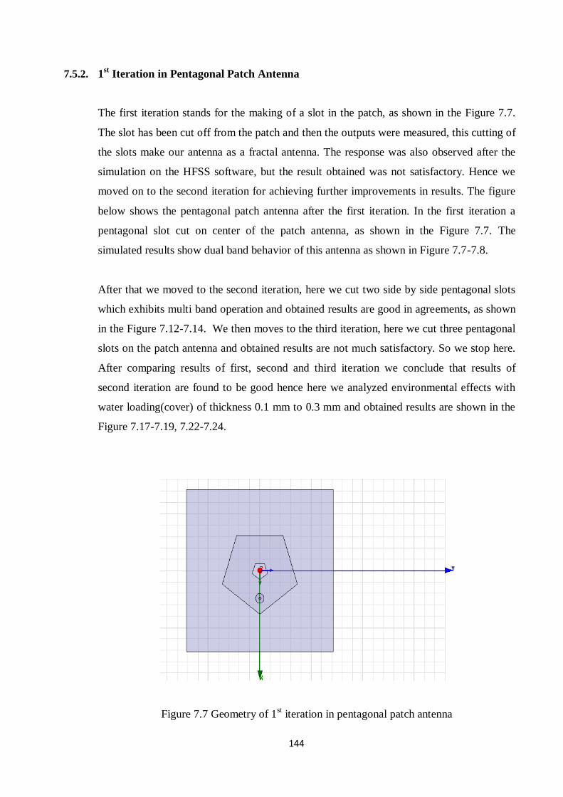
7.5.2. 1st Iteration in Pentagonal Patch Antenna

The first iteration stands for the making of a slot in the patch, as shown in the Figure 7.7.

The slot has been cut off from the patch and then the outputs were measured, this cutting of

the slots make our antenna as a fractal antenna. The response was also observed after the

simulation on the HFSS software, but the result obtained was not satisfactory. Hence we

moved on to the second iteration for achieving further improvements in results. The figure

below shows the pentagonal patch antenna after the first iteration. In the first iteration a

pentagonal slot cut on center of the patch antenna, as shown in the Figure 7.7. The

simulated results show dual band behavior of this antenna as shown in Figure 7.7-7.8.

After that we moved to the second iteration, here we cut two side by side pentagonal slots

which exhibits multi band operation and obtained results are good in agreements, as shown

in the Figure 7.12-7.14. We then moves to the third iteration, here we cut three pentagonal

slots on the patch antenna and obtained results are not much satisfactory. So we stop here.

After comparing results of first, second and third iteration we conclude that results of

second iteration are found to be good hence here we analyzed environmental effects with

water loading(cover) of thickness 0.1 mm to 0.3 mm and obtained results are shown in the

Figure 7.17-7.19, 7.22-7.24.

Figure 7.7 Geometry of 1st iteration in pentagonal patch antenna

145

In order to present the design procedure of achieving impedance matching for the first

iterated pentagonal patch antenna case, feed location is set at 11.1 mm and radius of the

patch is 19.107 mm. The radius for the iterated patch is 2.697 mm. After optimization we

met the design challenges such as return loss should be less than -10 dB, VSWR< 2 and

low spurious feed radiation.

Figure 7.8 Return loss vs frequency for 1st iteration

Figure 7.9 Input impedance vs frequency for 1st iteration

-24

-19

-14

-9

-4

1 2 3 4 5

S11, d

B

Frequency (GHz)

0

20

40

60

80

1 2 3 4 5 6 7

Z11,Ω

Frequency (GHz)

146

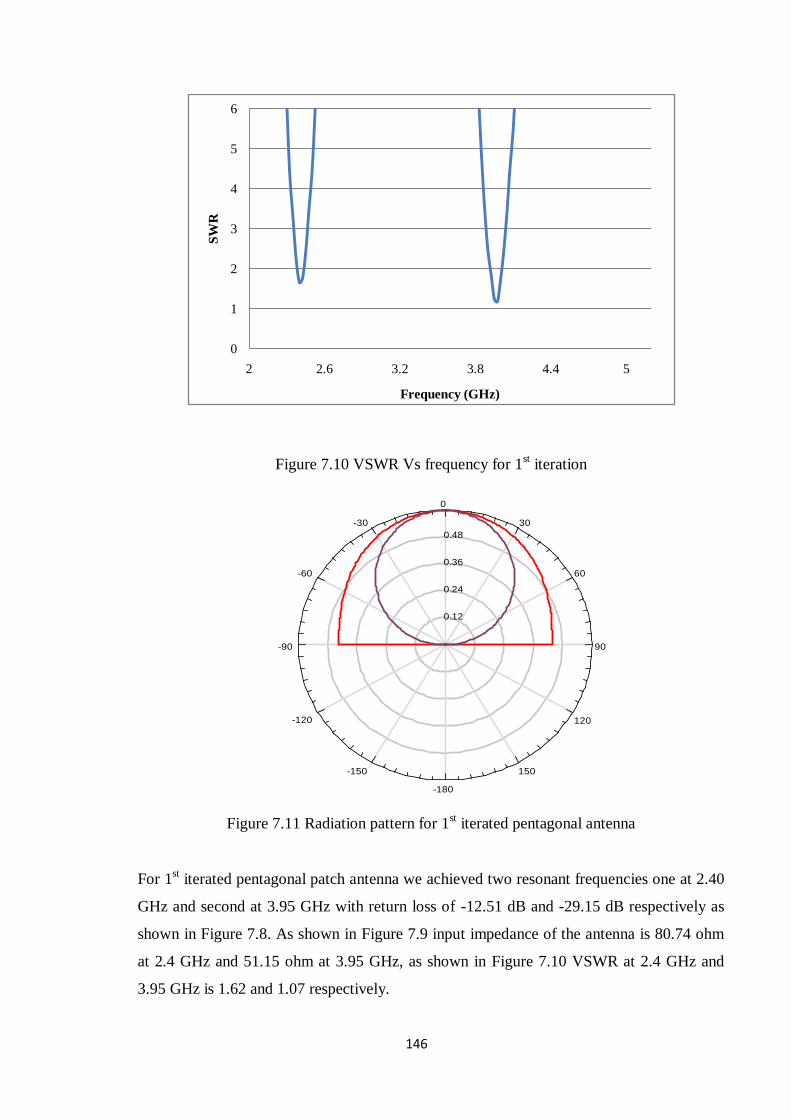
Figure 7.10 VSWR Vs frequency for 1st iteration

Figure 7.11 Radiation pattern for 1st iterated pentagonal antenna

For 1st iterated pentagonal patch antenna we achieved two resonant frequencies one at 2.40

GHz and second at 3.95 GHz with return loss of -12.51 dB and -29.15 dB respectively as

shown in Figure 7.8. As shown in Figure 7.9 input impedance of the antenna is 80.74 ohm

at 2.4 GHz and 51.15 ohm at 3.95 GHz, as shown in Figure 7.10 VSWR at 2.4 GHz and

3.95 GHz is 1.62 and 1.07 respectively.

0

1

2

3

4

5

6

2 2.6 3.2 3.8 4.4 5

SW

R

Frequency (GHz)

0.12

0.24

0.36

0.48

90

60

30

0

-30

-60

-90

-120

-150

-180

150

120

Ansoft Corporation HFSSDesign1Radiation Pattern 1

Curve Info

rETotal

Setup1 : LastAdaptive

Phi='0deg'

rETotal

Setup1 : LastAdaptive

Phi='90deg'

147

7.5.3. 2nd

Iteration in Pentagonal Patch Antenna

The second iteration stands for the making of two slots in the original patch, as shown in

the Figure 7.12 the slots has been cut off from the patch and then the outputs were

measured, this cutting of the slots make our antenna as a 2nd

iterated fractal patch antenna.

Figure 7.12 Geometry of 2nd

iteration in pentagonal patch antenna

The response was observed after the simulation on the HFSS software, but the result

obtained was satisfactory, even though we moved on to the third iteration for achieving

further improvements in results. The figure below shows the Pentagonal patch antenna after

the iteration. In order to present the design procedure for achieving impedance matching for

the second iterated pentagonal patch antenna case, feed location is set at 11.8 mm and

radius of the patch is 19.107 mm. The radius for both the iterated patch is 2.897 mm. After

optimization we met the design challenges such as return loss should be less than -10 dB,

VSWR < 2 and low spurious feed radiation.

Figure 7.13 Return loss vs frequency for 2nd

iteration

-30

-25

-20

-15

-10

-5

0

1 3 5 7 9

S11

(dB

)

Frequency (GHz)

148

Figure 7.14 VSWR vs frequency 2nd

iteration

Figure 7.15 impedance vs frequency for 2nd

iteration

Figure 7.16: Radiation pattern for 2nd

iterated pentagonal antenna

1

2

3

4

5

6

1.5 3.5 5.5 7.5 9.5

VS

WR

Frequency (GHz)

0

15

30

45

60

75

1 3 5 7 9

Z11,Ω

Frequency (GHz)

0.80

1.60

2.40

3.20

90

60

30

0

-30

-60

-90

-120

-150

-180

150

120

Ansoft Corporation HFSSDesign1Radiation Pattern 1

Curve Info

rETotal

Setup1 : LastAdaptive

Phi='0deg'

rETotal

Setup1 : LastAdaptive

Phi='90deg'

149

For 2nd

iterated pentagonal patch antenna we achieved three resonant frequencies, first at

2.16 GHz, second at 3.56 GHz and third at 7.92 GHz with return loss of -17.68 dB and -

21.51 dB and -41.11 dB respectively as shown in Figure 7.13. Above third resonant

frequency the variation in the stop band noise is quite large. As shown in Figure 7.15 input

impedance of the antenna is 62.94 ohm at 2.16 GHz, 46.63 ohm at 3.56 GHz and 49.12

ohm at 7.92 GHz.

7.5.4. 3rd

Iteration in Pentagonal Patch Antenna

The third iteration stands for the making of three slots in the original patch, as shown in the

figure 7.17 the slots has been cut off from the patch and then the outputs were measured.

This cutting of the slots make our antenna as a 3rd

iterated fractal patch antenna. The

response was observed after the simulation on the HFSS software, but the result obtained

was not satisfactory. Too much variation in results was there. So, we can conclude one

thing here that as the number of iterations goes beyond a limit, the performance of the

antenna decreases.

Figure 7.17 Geometry of 3rd

iteration in pentagonal patch antenna

150

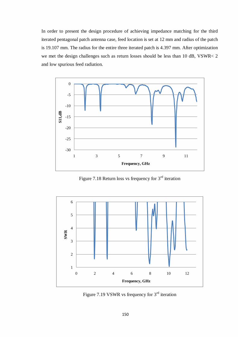
In order to present the design procedure of achieving impedance matching for the third

iterated pentagonal patch antenna case, feed location is set at 12 mm and radius of the patch

is 19.107 mm. The radius for the entire three iterated patch is 4.397 mm. After optimization

we met the design challenges such as return losses should be less than 10 dB, VSWR< 2

and low spurious feed radiation.

Figure 7.18 Return loss vs frequency for 3rd

iteration

Figure 7.19 VSWR vs frequency for 3rd

iteration

-30

-25

-20

-15

-10

-5

0

1 3 5 7 9 11

S11,d

B

Frequency, GHz

1

2

3

4

5

6

0 2 4 6 8 10 12

SW

R

Frequency, GHz

151

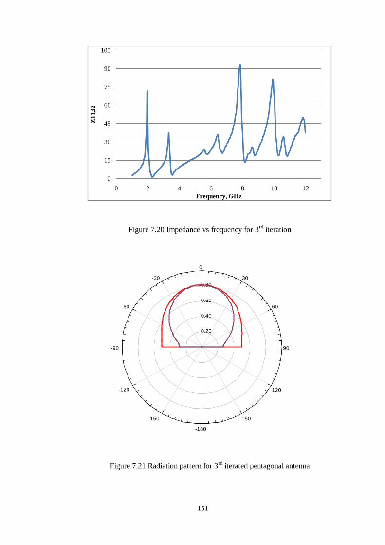
Figure 7.20 Impedance vs frequency for 3rd

iteration

Figure 7.21 Radiation pattern for 3rd

iterated pentagonal antenna

0

15

30

45

60

75

90

105

0 2 4 6 8 10 12

Z1

1,Ω

Frequency, GHz

0.20

0.40

0.60

0.80

90

60

30

0

-30

-60

-90

-120

-150

-180

150

120

Ansoft Corporation HFSSDesign1Radiation Pattern 1

Curve Info

rETotal

Setup1 : LastAdaptive

Phi='0deg'

rETotal

Setup1 : LastAdaptive

Phi='90deg'

152

Table 7.1 S11, Impedance and VSWR of the proposed fractal patch antenna

Types

Simulated

Frequency

(GHz)

S11(dB) Impedance

(Ω) SWR

0 Iteration 2.4375 -28.99 51.75 1.0736

1st Iteration

2.405 -12.16 82.06 1.6515

3.9775 -21.55 53.28 1.1824

2nd

Iteration

2.16 -16.39 67.31 1.3502

3.56 -18.14 39.03 1.2832

7.96 -27.62 48.2 1.0868

3rd

Iteration

1.96 -11.91 72.13 1.6795

3.36 -12.2 37.81 1.6506

7.96 -18.39 92.85 1.2734

10.08 -28.71 79.9 1.0761

Table 7.2 Simulated directivity, gain, radiated power and radiation efficiency of the

proposed fractal patch antenna

Iterations Directivity

(dB) Gain (dB)

Radiated power

(W)

Radiation

efficiency

0 Iteration 1.6 0.7491 0.005299 46.71%

1 Iteration 0.189 0.7366 0.0071 89.84%

2 Iteration 0.8385 0.55768 0.2908 85.66%

3 Iteration 0.7091 0.7183 0.0155 78.64%

For 3rd

iterated pentagonal patch antenna we achieved four resonant frequencies, first at

1.96 GHz, second at 3.36 GHz, third at 7.96 GHz and fourth at 10.08 GHz with return loss

of -11.91 dB, -12.20 dB, -18.39 dB and -28.71 dB respectively as shown in Figure 7.18.

153

The graph is not as sharp as in the case of first and second iteration. Ripples are very large

in the stop bands. As shown in Figure 7.20 input impedance of the antenna is 72.13 ohm at

1.96 GHz, 30.69 ohm at 3.36 GHz, 49.89 ohm at 7.96 GHz and 46.59 ohm at 10.08 GHz.

One can see too much variation in the input impedance from the graph. As shown in Figure

7.19 VSWR at resonant frequencies are 1.67, 1.65, 1.27 and 1.07 GHz respectively.

7.5.5. Fractal Patch Antenna with Dielectric Loading

Figure 7.22 Return loss variation vs frequency with accumulation of water

Figure 7.23 VSWR vs frequency variations with accumulation of water

-33

-28

-23

-18

-13

-8

-3

1 3 5 7 9

S11(d

B)

Frequency (GHz)

dB(S11) at t='0mm'

dB(S11) at t='0.1mm'

dB(S11) at t='0.2mm'

dB(S11) at t='0.3mm'

0

1

2

3

4

5

6

1.5 2.5 3.5 4.5 5.5 6.5 7.5 8.5 9.5

VS

WR

Frequency (GHz)

VSWR at t='0mm'

VSWR at t='0.1 mm'

VSWR at t='0.2 mm'

VSWR at t='0.3mm'

154

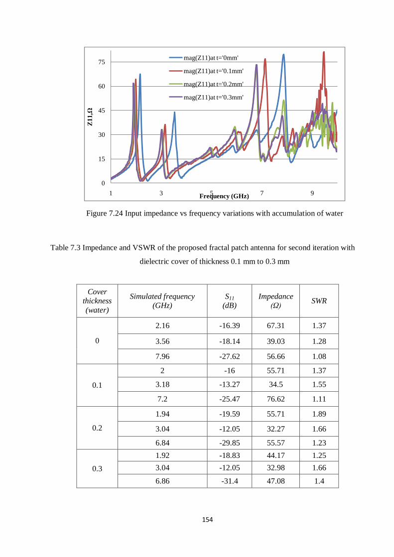
Figure 7.24 Input impedance vs frequency variations with accumulation of water

Table 7.3 Impedance and VSWR of the proposed fractal patch antenna for second iteration with

dielectric cover of thickness 0.1 mm to 0.3 mm

Cover

thickness

(water)

Simulated frequency

(GHz)

S11

(dB)

Impedance

(Ω) SWR

0

2.16 -16.39 67.31 1.37

3.56 -18.14 39.03 1.28

7.96 -27.62 56.66 1.08

0.1

2 -16 55.71 1.37

3.18 -13.27 34.5 1.55

7.2 -25.47 76.62 1.11

0.2

1.94 -19.59 55.71 1.89

3.04 -12.05 32.27 1.66

6.84 -29.85 55.57 1.23

0.3

1.92 -18.83 44.17 1.25

3.04 -12.05 32.98 1.66

6.86 -31.4 47.08 1.4

0

15

30

45

60

75

1 3 5 7 9

Z11,Ω

Frequency (GHz)

mag(Z11)at t='0mm'

mag(Z11)at t='0.1mm'

mag(Z11)at t='0.2mm'

mag(Z11)at t='0.3mm'

155

Table 7.4 Simulated directivity, gain radiated power and radiation efficiency of the proposed

fractal patch antenna for second iteration

With superstrate

Directivity 0.69

Gain 0.62

Radiated Power 0.112 W

Radiation Effect 89.83%

7.6. CONCLUSIONS

For the above simulated result for first, second, third iteration are tabulated in the Table 7.1

and 7.2, it is found that all the parameters of the antennas are satisfactory. After dielectric

loading results are tabulated in the Table 7.3 and 7.4 which reveal that the dielectric

loading can change all the parameter such as resonant frequency, return loss, impedance,

VSWR etc. of the patch antenna. It has been also observed that as the dielectric thickness

increases, the resonant frequency shift at lower side hence deteriorates the multi band

characteristics of the pentagonal patch antenna. As found, the main performances of the

patch antennas may be adversely affected if permittivity and thickness of the dielectric are

not chosen properly, hence next chapter is dedicated to look into opportunity to

compensate the effects of environmental conditions;. dielectric loading on the antenna

behaviors.

156

REFERENCES

1. Z. Baharav, ―Fractal arrays based on Iterated Functions System (IFS),‖ Antennas and

Propagation Society International Symposium, 1999, IEEE, Vol.4, pp- 2686 – 2689,

1999.

2. M.Navarro, J.M.Gonzlez. C.Puente, J.Romeu and A.Aguasca, ―Self-similar surface

current distribution on fractal Sierpinski antenna verified with infra-red thermograms,‖

Electronics Letters, Vol. 35, No. 17, pp.1393-1394, 19th Aug. 1999.

3. P. Felber, ―Fractal antennas -A literature study,‖ A project report for ECE 576 Illinois

Institute of Technology, January 16, 2001.

4. Sathya, ―Size reduction of low frequency microstrip patch antennas with Koch fractal

slots‖Mtech Thesis,IISC Banglore.

5. P.Hazdra, and M.Maz´anek , ―The miniature inverted Koch square microstrip patch

antenna,‖ Proceedings of ISAP2005, Seoul, Korea pp.121-124,2005.

6. V.Gupta and N. Gupta , ―Two compact microstrip patch antennas for 2.4 GHz band – a

comparison,‖ Microwave Review, pp. 29-31, November, 2006.

7. V. R. Gupta and N. Gupta, ―Analysis of a fractal microstrip patch antenna,‖ International

Journal of Microwave And Optical Technology, Vol. 2, No. 2, pp. 124-129, April 2007.

8. F.H. Kashani et al, ―A novel broadband fractal Sierpinski shaped, microstrip antenna,‖

Progress in Electromagnetics Research, Vol. 4, 179–190, pp. 179-190, 2008.

9. A. Azari, ―Ultra wideband fractal microstrip antenna design,‖ Progress Electromagnetics

Research , Vol. 2, 7-12, 2008.

10. J. F. Jibrael

and M. H. Hammed, ―A new multiband patch microstrip plusses fractal antenna

for wireless applications,‖ ARPN Journal of Engineering and Applied Sciences, Vol. 5,

No. 8, pp.17-21, August 2010.