Persistence Barcodes for Shapes

Eurographics Symposium on Geometry Processing (2004)R. Scopigno, D. Zorin, (Editors)

Persistence Barcodes for Shapes

Gunnar Carlsson†, Afra Zomorodian‡§, Anne Collins†, and Leonidas Guibas‡

† Department of Mathematics‡ Department of Computer Science

Stanford University

AbstractIn this paper, we initiate a study of shape description and classification via the application of persistent homol-ogy to two tangential constructions on geometric objects. Our techniques combine the differentiating power ofgeometry with the classifying power of topology. The homology of our first construction, the tangent complex,can distinguish between topologically identical shapes with different “sharp” features, such as corners. To cap-ture “soft” curvature-dependent features, we define a second complex, the filtered tangent complex, obtained byparametrizing a family of increasing subcomplexes of the tangent complex. Applying persistent homology, we ob-tain a shape descriptor, called a barcode, that is a finite union of intervals. We define a metric over the space ofsuch intervals, arriving at a continuous invariant that reflects the geometric properties of shapes. We illustrate thepower of our methods through a number of detailed studies of parametrized families of mathematical shapes.

1. Introduction

In this paper, we initiate a study of shape description usinga marriage of geometric and topological techniques. For us,a shape is any closed subset of a Euclidean space. Questionswe wish to answer include:

• Which shapes are identical up to a rigid motion of theambient Euclidean space?

• Which shapes belong to certain classes of shapes? For in-stance, we may wish to distinguish the class of rectangularprisms form the class of tetrahedra, or the class of ellip-soids from the class of spheres.

• Which shapes are identical up to a smooth diffeomor-phism of the ambient Euclidean space? This is a coarseclassification.

• What are the features of the shape? For example, thesefeatures could be singular points of various types.

We attempt to obtain information about shapes through dif-ferent levels of classification, from fine to coarse. One can

† Research supported, in part, by NSF under grant DMS 0101364.‡ Research supported, in part, by NSF/DARPA under grantCARGO 0138456 and NSF under grant ITR 0086013.§ Portion done while author was visiting the Max-Planck-Institutfür Informatik in Saarbrücken, Germany.

view geometry as the finest level of classification as it fo-cuses on local properties of shapes. In this sense, geometryhas a quantitative nature and can answer low level questionsabout a shape. But all our questions have a qualitative feeland take a higher view of a shape. This prompts us to lookat topological techniques which classify shapes accordingto the way they are connected globally – their connectiv-ity. Unfortunately, this view is often too coarse to be useful.For example, the topological invariant homology classifiesshapes according to the number of components, tunnels, andenclosed spaces. This classification cannot distinguish be-tween circles and ellipses, between circles and rectangles, oreven between Euclidean spaces of different dimensions. Fur-ther, it cannot identify sharp features, such as corners, edges,or cone points: their neighborhoods are all homeomorphic orconnected the same way. Whereas geometry is too sensitivefor shape description, topology seems to be too insensitive.We seek to enrich topological techniques with the geomet-ric content of a shape so that our methods manifest moderatesensitivity. We need a method that combines local and globalinformation to characterize a shape.

1.1. Approach

In this paper, we propose a robust method that combines thedifferentiating power of geometry with the classifying power

c© The Eurographics Association 2004.

Carlsson et al. / Persistence Barcodes for Shapes

of topology. We apply homology not to a space X itself, butto derived spaces that have richer geometric content. In thiscase, we construct spaces out of X using tangential infor-mation about X as a subset of R

n. We define two tangentialconstructions: the tangent complex and the filtered tangentcomplex. The tangent complex is the closure of the space ofall tangents to all points of X . The homology of this complexcan detect many sharp features of X , such as edges and cor-ners. However, if the two shapes differ only in soft features,their tangent complexes are topologically indistinguishable.For example, an ellipse differs from a circle in having a rangeof curvatures, a feature not reflected in the ellipse’s tangents.

For even more differentiating power, we enrich our tan-gent complex with information about the curvature of thespace at each point. The resulting filtered tangent complexis actually an increasing family of spaces, parametrized bycurvature. Applying homology to this family, we obtain aninvariant called a persistence module that yields subtler in-formation about a shape, such as the existence of regions oflow or high curvature. The filtered tangent complex can dis-tinguish a circle from an ellipse, even though these spacesare homeomorphic and have homeomorphic tangent com-plexes. We provide a number of examples to illustrate thepower of our tangential constructions.

We also define a simple shape descriptor that arises frompersistent homology and carries information about a shape.We call this combinatorial invariant a barcode as it is simplya finite collection of intervals on the right half line. To com-pare barcodes, we define a metric on the set of barcodes. Wemay now use clustering techniques on the metric space ofbarcodes for shape recognition and classification.

In this paper, we deal with explicit calculations for geo-metric objects to demonstrate the sensitivity of our invari-ants to properties of shapes, and their effectiveness in shaperecognition. Our main interest, however, is computational.We wish to obtain information about a shape when we onlyhave a finite set of samples from that shape. Such a setof points, commonly called point cloud data or PCD forshort, is a discrete topological space. We are faced, there-fore, with the additional difficulty of recovering the underly-ing shape topology, as well as approximating the tangentialspaces we define. These issues extend well beyond the scopeof this paper. Our goal here is to examine the viability of ourtechniques in an ideal mathematical setting, where we havefull information about the spaces considered. We make noclaims, however, about the direct applicability of the resultsof this paper to the PCD domain, which we have addressedfor PCDs of curves in [CZCG04].

1.2. Background and Prior Work

Distinguishing and recognizing shapes is a well-studiedproblem in many areas of computer science, such as vi-sion, pattern recognition, and graphics [Fan90, Fis89]. Me-

dial axis techniques have been extensively used for this pur-pose [ZY96]. One particular aspect of this problem is under-standing “shape spaces” in their entirety [Boo91, KBCL99].For instance, one may study a shape space from a differen-tial point of view [LPM01]. Broadly speaking, most methodstry to coordinatize the shape space in a way that gives usefulcombinatorial information about the space.

The idea of applying homology to derived spaces is a fa-miliar one within topology. Some applications include theclassification of vector bundles [MS74], and Donaldson the-ory, which constructs invariants of smooth structures on ho-motopy equivalent four-dimensional manifolds, using mod-uli spaces of self-dual connections [DK90]. The tangentialcomplexes we study are familiar in geometric measure the-ory [Fed69]. Morse theory analyzes the topology of a spaceby utilizing increasing families of spaces [Mil63]. Persistenthomology was first defined for topological simplification ofalpha shapes [ELZ02]. It was then extended to arbitrary d-dimensional spaces and arbitrary fields of coefficients usinga classification result [ZC04]. The latter paper also intro-duced the notion of using intervals as homological invari-ants.

1.3. Overview

We organize the rest of the paper as follows. We describea topological construction that we employ in this paper inSection 2. We also list some tools we utilized in our calcu-lations. In Section 3, we define our first derived complex,the tangent complex, based on the notion of the tangent conefrom geometric measure theory. We also discuss a numberof examples that point out the strengths and weaknesses ofthe complex in shape recognition. This discussion motivatesour second derived complex in Section 4, the filtered tangentcomplex, which is more sensitive and can detect curvature-dependent features. Once again, we study a number of ex-amples in two and three dimensions. Section 5 introducespersistent homology and the classification it gives in termsof barcodes. It also defines a metric on the space of barcodesand gives an algorithm for computing this metric based onweighted bipartite matching. In Section 6, we revisit our ex-amples from Sections 3 and 4 and compute their homol-ogy or persistent homology, drawing the barcodes in thelatter cases. We devote Section 7 to an extended example,where we illustrate the effect of varying parameters on thebarcodes and the distance between shapes by studying theparametrized families of a glass and a bottle. We concludethe paper with some preliminary results from our softwareto compute tangent complexes for PCDs.

2. Algebraic Topology

We assume that the reader is familiar with major con-cepts from algebraic topology, such as homotopy, homotopyequivalence, homology, and Meyer-Vietoris sequences. For



these definition see any standard text in the area, such asGreenberg and Harper [GH81] or Hatcher [Hat01].

We mention a space-level construction we will be usinglater in this paper. Intuitively, when a space is broken into aunion of two pieces, we can express it via the constructionof gluing the two pieces together along a subspace.

Definition 1 (A ∪X B) Suppose we have a space X, togetherwith inclusions f : X ↪→ A and g : X ↪→ B. Then, we mayconstruct a new space as the quotient of the disjoint union ofA and B,

A ∪X B = A ∪̇X ∪̇B/∼,

where ∼ is the equivalence relation generated by the equiv-alences x ∼ f (x) ∈ A, and x ∼ g(x) ∈ B, for all x ∈ X. Simi-larly, if we have inclusions f : X ↪→A, g : X ↪→B, h : Y ↪→B,and k : Y ↪→C, we define

A ∪X B ∪Y C = (A ∪X B) ∪Y C.

Although this construction depends on the inclusions f andg, they are not indicated in the notation.

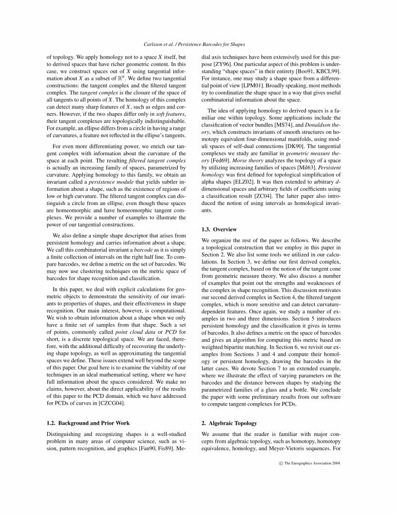
Example 1 (glass) Figure 1 shows the construction of aglass shape from two pieces. The side is a cylinder A =S1× [0,1] and the bottom is a disc B = D2. We use the dashedcircle X = S1 to glue the two spaces together, resulting inD2 ∪S1 (S1 × [0,1]), which looks like a glass or the bottomof a bottle.

Figure 1: The cylinder S1 × [0,1] and the disc D2 areglued together along the dashed circles. The resulting spaceD2 ∪S1 (S1× [0,1]) has the same geometry as a glass or bot-tom of a bottle.

3. The Tangent Complex

In this section, we introduce the first of our tangential con-structions, the tangent complex for a subset of R

n. Our con-struction is closely related to the concept of the tangent cone,defined in geometric measure theory [Fed69]. After definingthe complex, we give a number of examples for intuition.

Definition 2 (tangent complex) Let X be any subset of Rn.

We define T 0(X) ⊆ X ×Sn−1 to be

T 0(X) =

{

(x,ζ) | limt→0

d(x+ tζ,X)

t= 0}

.

The tangent complex of X is the closure of T 0, T (X) =

T 0(X) ⊆ X ×Sn−1. T (X) comes equipped with a projectionπ : T (X) → X that projects a point (x,ζ) ∈ T (X) in the tan-gent complex onto its basepoint x, and T (X)x = π−1(x) ⊆T (X) is the fiber at x.

Informally, (x,ζ) represents a tangent vector at a point x∈ X ,if the ray beginning at x and pointing in the direction pre-scribed by ζ approaches X faster than linearly. There is alsoa projection ω : T (X)→ Sn−1 that projects all the fibers ontothe (n−1)-sphere. We have the following useful propositionconcerning this construction.

Proposition 1 Suppose that x ∈ X is a smooth point of X,so that there is a neighborhood U ⊆ R

n of x and a smoothfunction f : U → R

m, such that

• U ∩X = f−1(0), and• the Jacobian of f , D f (ξ), has rank m for every ξ in U.

Then T (X)x ∼= Sn−m−1

For intuition, we next give a number of examples. We willrevisit these examples in Section 6 to discuss the homologyof their tangent complexes. We begin with one-dimensionalobjects, as they are easier to work with, given the definition.

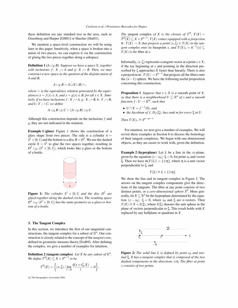
Example 2 (hyperplane) Let L be a line in the xy-plane,given by the equation (x−x0) ·ξ = 0, for point x0 and vectorξ. Then we have ω(T (L)) = {±η}, where η is a unit vectorperpendicular to ξ, and

T (L) ∼= L×{±η}.

We show the line and its tangent complex in Figure 2. Thearrows on the tangent complex components give the direc-tions of the tangents. The fiber at any point consists of twodistinct points, or a zero-dimensional sphere S0. More gen-erally, let X ⊆R

n be the hyperplane determined by the equa-tion (x − x0) · ξ = 0, where x0 and ξ are n-vectors. ThenT (X) ∼= X ×S(ξ), where S(ξ) denotes the unit sphere in theplane of vectors perpendicular to ξ. This result holds with Xreplaced by any halfplane or quadrant in X .

x L

−η

+η

x0

ξ

Figure 2: The solid line L is defined by point x0 and nor-mal ξ. It has a tangent complex that is composed of the twodashed components in the directions ±η. The fiber at pointx consists of two points.



Example 3 (vee) Consider a space X ⊆ R2 that looks like

a ‘V’, as shown in Figure 3. Formally, X = (R+ × 0) ∪(0×R+). We evaluate the fibers T (X)x directly. The fiberat any smooth point is S0 as in the previous example. Forpoints along the x-axis, the two points will be (x,(1,0)) and(x,(−1,0)), and along the y-axis, they will be (x,(0,1)) and(x,(0,−1)). At the origin O, however, the fiber T (X)O con-sists of four points, namely (O,(±1,0)) and (O,(0,±1)).We can easily verify that the tangent complex is actually theunion of two pieces, the tangent complexes of the two factorsof the space:

T (R+ ×0) = (R+ ×0)×{(±1,0)},

T (0×R+) = (0×R+)×{(0,±1)}.

So that the entire complex is:

T (X) = (R+ ×0)×{(±1,0)} ∪ (0×R+)×{(0,±1)}.

It is easy to see that this space is a disjoint union of fourdistinct half lines, as shown in Figure 3.

O

y x

Figure 3: Solid ‘V’ space X has a tangent complex T (X)that is composed of the four dashed components.

The features detected by homology of the tangent com-plex are sharp features: they are unaffected by smooth dif-feomorphisms of the ambient space R

n. However, we areoften interested in soft features that are characterized bychanges in curvature. We give two examples of the kindsof features we would like to capture.

Example 4 (circle vs. ellipse) Consider the difference be-tween a circle and an ellipse. They are topologically thesame and have no sharp features. There is, however, a dif-ference in the lengths of the axes in the case of the ellipsethat distinguishes it from the circle.

Example 5 (bottle vs. glass) Consider the difference be-tween a bottle and a glass. Again, they are topologically thesame and even have a common sharp feature: the circularrim at the bottom. But a bottle has a narrow neck that a glassdoes not have. Of course, bottles have many different shapes,but they all share this basic difference with a glass.

The distinctions above cannot be detected via homologydirectly, as the spaces are homeomorphic. They cannot be

detected by the tangent complex, either, as the objects areobtainable from each other by smooth deformations of theambient space. Rather, they require more a sophisticatedconstruction which we introduce in the next section.

4. The Filtered Tangent Complex

In this section, we define a second construction based on tan-gential information: the filtered tangent complex. We devotethe bulk of this section to detailed examples, building thecomplex for interesting families of subspaces of the two- andthree-dimensional Euclidean spaces. We will revisit theseexamples in Section 6, when we apply persistent homologyto arrive at compact shape descriptors.

4.1. Definition

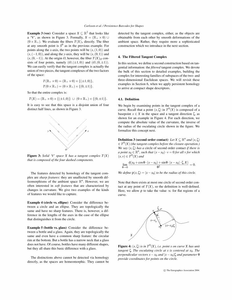
We begin by examining points in the tangent complex of acurve. Recall that a point (x,ζ) in T 0(X) is composed of abasepoint x ∈ X in the space and a tangent direction ζ, asshown for an example in Figure 4. For each direction, wecompute the absolute value of the curvature, the inverse ofthe radius of the osculating circle shown in the figure. Weformalize this concept next.

Definition 3 (second order contact) Let X ⊆ Rn and (x,ζ)

∈ T 0(X) (the tangent complex before the closure operation.)We say (x,ζ) has a circle of second order contact if there isa point x0 ∈ R

n, such that (x− x0) · v = 0 for all v for which(x,v) ∈ T 0(X) and

limθ→0

d(x0 + cosθ · (x− x0)+ sinθ · |x− x0| ·ζ,X)

θ2 = 0.

We define ρ(x,ζ) = |x− x0| to be the radius of this circle.

Note that there exists at most one circle of second order con-tact at any point of T (X), so the definition is well-defined.Here, we allow ρ to take the value ∞ for flat regions of acurve.

x−x0

0x ζx−x| |0

xζ

X

θ

Figure 4: (x,ζ) is in T 0(X), i.e. point x on curve X has unittangent ζ. The osculating circle at x is centered at x0. Theperpendicular vectors x− x0 and |x− x0|ζ and parameter θprovide coordinates for points on the circle.



Definition 4 (filtered) Let T 0δ (X) to be the set of points

(x,ζ) ∈ T 0(X) for which the circle of second order con-tact exists with δ ≥ 1/ρ(x,ζ). Let Tδ(X) be the closure ofT 0

δ (X) in Rn × Sn−1. We call the δ-parametrized family of

spaces {Tδ(X)}δ≥0 the filtered tangent complex, denoted byT filt(X).

In other words, we allow tangent complex points to enterthe complex according to the curvature at their associatedbasepoints. If δ ≤ δ′, we have an inclusion Tδ(X) ⊆ Tδ′(X),so the complexes are properly nested. As before, we denoteTδ(X)x = π−1

δ (x), where πδ : Tδ(X) → X is the natural pro-jection. It is the topological structure of T filt(X) that carriesinformation about the soft features of the underlying space.

4.2. Examples: Curves

We elucidate these concepts through examples in the rest ofthis section. We begin with one-dimensional subsets of R

2,or curves.

Example 6 (circle) Let X be the circle of radius R centeredat the origin in the plane. The full tangent complex T (X) ishomeomorphic to S1×S0, as there are two tangent directionsat each point. Every point (x,ζ) ∈ T 0(X) admits a circle ofsecond order contact, namely X itself, so ρ(x,ζ) = R for all(x,ζ). Therefore,

Tδ(X) =

{

∅, for δ < 1/R,T (X), for δ ≥ 1/R.

Example 7 (ellipse) Let X be the ellipse given by the equa-tion x2

a2 + y2

b2 = 1. Since X is a smooth manifold, every(x,ζ) admits a circle with second order contact. We recallthat the formula for the radius of the osculating circle to aparametrized curve ϕ(t) = (x(t),y(t)) is given by

|ϕ′(t)|3

|x′(t)y′′(t)− x′′(t)y′(t)|.

A parametrization for the ellipse X is given by ϕ(t) =(acos(t),bsin(t)). Direct computation shows that at thepoint ϕ(t), ρ is given by

(a2 +(b2 −a2)cos2(t))32

ab,

for both tangent directions. Without loss of generality, weassume b > a > 0. Then, ρ attains its maximum value ofb2/a at t ∈ {0,π}, and its minimum value of a2/b at t ∈{π/2,3π/2}.

Moreover, ρ is decreasing as t increases in intervals(

0, π2)

and(

π, 3π2

)

, and increasing in intervals( π

2 ,π)

and(

3π2 ,2π

)

. Therefore, the filtered tangent complex behavesas follows. For each case, there is a corresponding illustra-tion in Figure 5.

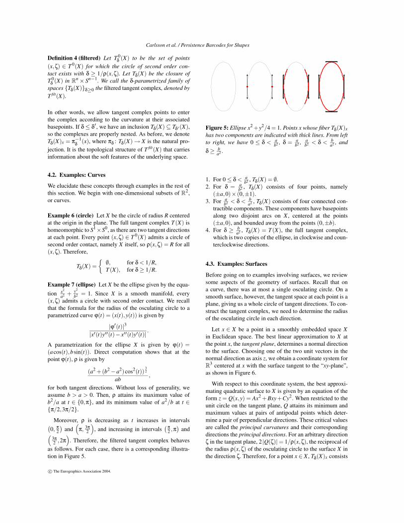
Figure 5: Ellipse x2 +y2/4 = 1. Points x whose fiber Tδ(X)xhas two components are indicated with thick lines. From leftto right, we have 0 ≤ δ < a

b2 , δ = ab2 , a

b2 < δ < ba2 , and

δ ≥ ba2 .

1. For 0 ≤ δ < ab2 , Tδ(X) = ∅.

2. For δ = ab2 , Tδ(X) consists of four points, namely

(±a,0)× (0,±1).3. For a

b2 < δ < ba2 , Tδ(X) consists of four connected con-

tractible components. These components have basepointsalong two disjoint arcs on X , centered at the points(±a,0), and bounded away from the points (0,±b).

4. For δ ≥ ba2 , Tδ(X) = T (X), the full tangent complex,

which is two copies of the ellipse, in clockwise and coun-terclockwise directions.

4.3. Examples: Surfaces

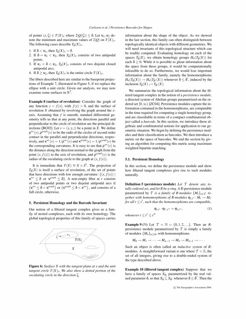
Before going on to examples involving surfaces, we reviewsome aspects of the geometry of surfaces. Recall that ona curve, there was at most a single osculating circle. On asmooth surface, however, the tangent space at each point is aplane, giving us a whole circle of tangent directions. To con-struct the tangent complex, we need to determine the radiusof the osculating circle in each direction.

Let x ∈ X be a point in a smoothly embedded space Xin Euclidean space. The best linear approximation to X atthe point x, the tangent plane, determines a normal directionto the surface. Choosing one of the two unit vectors in thenormal direction as axis z, we obtain a coordinate system forR

3 centered at x with the surface tangent to the “xy-plane”,as shown in Figure 6.

With respect to this coordinate system, the best approxi-mating quadratic surface to X is given by an equation of theform z = Q(x,y) = Ax2 + Bxy +Cy2. When restricted to theunit circle on the tangent plane, Q attains its minimum andmaximum values at pairs of antipodal points which deter-mine a pair of perpendicular directions. These critical valuesare called the principal curvatures and their correspondingdirections the principal directions. For an arbitrary directionζ in the tangent plane, 2 |Q(ζ)|= 1/ρ(x,ζ), the reciprocal ofthe radius ρ(x,ζ) of the osculating circle to the surface X inthe direction ζ. Therefore, for a point x ∈ X , Tδ(X)x consists



of points (x,ζ) ∈ T (X)x where 2|Q(ζ)| ≤ δ. Let κ1,κ2 de-note the minimum and maximum values of 2|Q| on T (X)x.The following cases describe Tδ(X)x.

1. If δ < κ1, then Tδ(X)x = ∅.2. If δ = κ1 < κ2, then Tδ(X)x consists of two antipodal

points.3. If κ1 < δ < κ2, Tδ(X)x consists of two disjoint closed

antipodal arcs.4. If δ ≥ κ2, then Tδ(X)x is the entire circle T (X)x.

The fibers described here are similar to the basepoint projec-tions of Example 7, illustrated in Figure 5, if we replace theellipse with a unit circle. Given our analysis, we may nowexamine some surfaces in R

3.

Example 8 (surface of revolution) Consider the graph ofany function y = f (x), with f (x) > 0, and the surface ofrevolution X obtained by revolving the graph around the x-axis. Assuming that f is smooth, standard differential ge-ometry tells us that at any point, the directions parallel andperpendicular to the circle of revolution are the principal di-rections [BG92]. Let v = (x,y,z) be a point in X . We defineρrev(v),ρgraph(v) to be the radii of the circles of second ordercontact in the parallel and perpendicular directions, respec-tively, and κrev(v) = 1/ρrev(v) and κgraph(v) = 1/ρgraph(v) bethe corresponding curvatures. It is easy to see that ρrev(v) isthe distance along the direction normal to the graph from thepoint (x, f (x)) to the axis of revolution, and ρgraph(v) is theradius of the osculating circle to the graph at (x, f (x)).

It is immediate that T (X) ∼= X × S1. The projection ofTδ(X) is itself a surface of revolution, of the set of pointsthat have directions with low enough curvature: {(x, f (x)) |κrev ≤ δ or κgraph ≤ δ}. A non-empty fiber at v consistsof two antipodal points or two disjoint antipodal arcs if(

κrev ≤ δ < κgraph) or(

κgraph ≤ δ < κrev) , and consists of afull circle, otherwise.

5. Persistent Homology and the Barcode Invariant

Our notion of a filtered tangent complex gives us a fam-ily of nested complexes, each with its own homology. Theglobal topological properties of this family of spaces carries

X

ζT(X)x

x

Figure 6: Surface X with the tangent plane at x and the unittangent circle T (X)x. We also show a dotted portion of theosculating circle in the direction ζ.

information about the shape of the object. As we showedin the last section, this family can often distinguish betweentopologically identical objects with different geometries. Wewill need invariants of this topological structure which canbe readily computed. Evaluating homology on each of thespaces Tδ(X), we obtain homology groups Hn(Tδ(X)) foreach δ ≥ 0. While it is possible to glean information aboutthe space from these groups, it would be computationallyinfeasible to do so. Furthermore, we would lose importantinformation about the family, namely the homomorphismsHn(Tδ(X)) → Hn(Tδ′(X)) whenever δ ≤ δ′, induced by theinclusion Tδ(X) ↪→ Tδ′(X).

We summarize the topological information about the fil-tered tangent complex in the notion of a persistence module,a directed system of Abelian groups parametrized on the or-dered set [0,∞) [ZC04]. Persistence modules capture the in-formation contained in the homomorphisms, are computablein the time required for computing a single homology group,and are classifiable in terms of a compact combinatorial ob-ject called a barcode. In this section, we introduce these al-gebraic and combinatorial notions for application to our ge-ometric situation. We begin by defining the persistence mod-ules and their classification as barcodes. We then introduce ametric on the space of barcodes. We end the section by giv-ing an algorithm for computing this metric using maximumweighted bipartite matching.

5.1. Persistent Homology

In this section, we define the persistence module and showhow filtered tangent complexes give rise to such modulesnaturally.

Definition 5 (persistence module) Let T denote any to-tally ordered set, and let R be a ring. A R-persistence moduleparametrized by T is a family of R-modules {Mt}t∈T to-gether with homomorphisms of R-modules ϕt,t′ : Mt → Mt′

for all t ≤ t′, such that the homomorphisms are compatible,

ϕt,t′ ·ϕt′,t′′ = ϕt,t′′ , (1)

whenever t ≤ t′ ≤ t′′

Example 9 (N) Let T = N = {0,1,2, . . .}. Then an R-persistence module parametrized by T is simply a familyof modules {Mn}n≥0, with homomorphisms

M0 → M1 → ·· · → Mn−1 → Mn → Mn+1 → ·· · .

Such an object is often called an inductive system of R-modules. A straightforward variant is one where T = Z, theset of all integers, giving rise to a double-ended system ofthe type described above.

Example 10 (filtered tangent complex) Suppose that wehave a family of spaces Xδ, parametrized by the real val-ued parameter δ, so that Xδ ⊆ Xδ′ whenever δ ≤ δ′. Then the



family of Abelian groups Hn(Xδ,G), where G is any Abeliangroup, is a G-persistence module parametrized by R. Notethat if G is any field, then we obtain a G-persistence vectorspace parametrized by R over the field G.

We also speak of a persistence chain complexparametrized by T over a ring R, a family of chaincomplexes {C t

∗}t∈T of G-modules together with chainmaps C t

∗ → C t′∗ whenever t ≤ t′, satisfying the analogues

of the compatibility relations (1) above. The homology ofa persistence complex parametrized by T over G is alwaysa G-persistence module, parametrized by T . There areanalogous notions of homomorphism and isomorphism forpersistence modules. We are mainly concerned with theclassification, up to isomorphism, of persistence modulesover fields.

5.2. Classification over Fields

We first consider persistence modules {Vt}t∈N parametrizedby N over a field F . We are able to classify these mod-ules, provided they are finite. Precisely, a persistence module{Vt}t parametrized by N over F is of finite type if

1. each vector space Vt is finite dimensional, and2. there is an integer N so that for all t ≥ N, ϕN,t are isomor-

phisms.

Given any pairs of integers (m,n) with m ≤ n, we define thepersistence module Q(m,n) over N by

Q(m,n)t =

{

0, if t < m or t ≥ n,F, otherwise,

The homomorphisms ϕi j are the identity homomorphismsfor m ≤ i ≤ j ≤ n. We can trivially extend this definition tothe case n = +∞. The main result of [ZC04] is the follow-ing.

Proposition 2 (classification) A persistence moduleparametrized by N over F of finite type is isomorphic to oneof the form

n⊕

s=1Q(is, js),

where js can be +∞, and the decomposition is unique up tothe order of the pairs.

This result is a consequence of the fundamental theorem forfinitely generated modules over the graded principal idealdomains (PID) F[t], with t having degree 1. Using the Artin-Rees construction, we can show that persistence modulesparametrized by N over any ring R are characterized by anassociated graded module (non-negatively graded) over R[t],and the result follows by taking R = F . We note this sim-ple classification does not extend to non-fields, as the gradedR[t] will not be a PID.

We can achieve similar results for other parameter spacesusing suitable finiteness conditions. For example, if T = R,we say a persistence module {Vs}s over F is of finite type ifthere are a finite number of unique finite-dimensional vectorspaces in the persistence module. Let I be an interval. Wedefine a persistence vector space Q(I) over F

Q(I)s =

{

0, if s 6∈ I,F, otherwise,

where the homomorphism is the identity within each inter-val. We can now state an analog of Proposition 2.

Proposition 3 A persistence module parametrized by R

over F of finite type is isomorphic to one of the formn⊕

s=1Q(Is),

where each interval Is is bounded from below, and the de-scription is unique up to the order of the intervals.

5.3. Metric Space of Barcodes

In the last section, we saw that we can classify persistencemodules parametrized by N with using a number of pairs ofintegers {(is, js)}s. If we view these pairs as half-open in-tervals {[is, js)}s, the description matches that of modulesparametrized by R. This family of intervals is our shape de-scriptor.

Definition 6 (barcode) A barcode is a finite set of intervalsthat are bounded below.

Intuitively, the intervals denote the life-times of a non-trivialloop in a growing complex. The left endpoint signifies thebirth of a new topological attribute, and the right endpointsignals its death. The longer the interval, the more importantthe topological attribute, as it insists on being a feature of thecomplex.

We next wish to form a metric space over the collection ofall barcodes. We do so using a quasi-metric, a metric that has∞ as a possible value, where x+∞ = ∞ and ∞+∞ = ∞.Let I denote the collection of all possible barcodes. We wishto define a quasi-metric D(S1,S2) on all pairs of barcodes(S1,S2), with S1,S2 ∈ I, so that if we move the endpoint ofany single interval in either set by a dissimilarity ε, D(S1,S2)changes by no more than ε. Let I,J be any two intervals ina barcode. We define their dissimilarity δ(I,J) to be theirsymmetric difference: δ(I,J) = µ(I ∪ J− I ∩ J), where µ de-notes one-dimensional measure. Note that δ(I,J) may be in-finite. Given a pair of barcodes S1 and S2, a matching is aset M(S1,S2) ⊆ S1 × S2 = {(I,J) | I ∈ S1 and J ∈ S2}, sothat any interval in S1 or S2 occurs in at most one pair (I,J).Let M1,M2 be the intervals from S1,S2, respectively, thatare matched in M, and let N be the non-matched intervalsN = (S1 −M1)∪ (S2 −M2). Given a matching M for S1 and



S2, we define the distance of S1 and S2 relative to M to bethe sum

DM(S1,S2) = ∑(I,J)∈M

δ(I,J)+ ∑L∈N

µ(L).

We now look for the best possible matching to define thequasi-metric.

Definition 7 (metric) D(S1,S2) = minM DM(S1,S2).

For a pair (I,J), we know that δ(I,J) = µ(I) + µ(J)−2µ(I∩J). Now, for any matching M, we define the similarityof S1 and S2 with respect to M to be

SM(S1,S2) = ∑(I,J)∈M

µ(I ∩ J)

=12

(

∑S1

µ(I)+∑S2

µ(J)−DM(I,J)

)

.

Minimizing DM is equivalent to maximizing SM . We maydo the latter by recasting the problem as a graph problem.Given sets S1 and S2, we define G(V,E) to be a weighted bi-partite graph [CLRS01]. We place a vertex in V for each in-terval in S1 ∪S2. We place an edge in E for each pair (I,J)∈S1 × S2 with weight µ(I ∩ J). Maximizing SM is equivalentto the well-known maximum weight bipartite matching prob-lem. We may utilize one of several algorithms for computingthe matching, such as the Hungarian algorithm with timecomplexity O(|V ||E|) [Kuh55], or the Gabow-Tarjan algo-rithm with complexity O(

√

|V ||E| log |E|) [GT89].

6. Examples, Revisited

Having described persistent homology, in this section we re-visit all of our examples from sections 3 and 4. We give pre-cise descriptions of the homology groups, and in the case ofthe filtered complexes, we provide pictures of the barcodesthat describe the persistence modules.

Example 11 (hyperplane) For the hyperplane X in Exam-ple 2, we found that the tangent complex has the formX × Sn−1. Since X is contractible, we may use the Kün-neth formula to conclude that H∗(T (X)) ∼= H∗(Sn−1). Welist Hi(T (X)) in the following table, where the dimension islisted horizontally, and i maps to dimensions not accountedfor.

0 i n−1Z 0 Z

The Betti numbers are the dimensions of these vector spaces,so β0(T (X)) = βn−1(T (X)) = 1 and βi(T (X)) = 0, for i 6=0,n− 1. In the remaining examples, we do not list the Bettinumbers explicitly, as they can be easily read off.

Example 12 (vee) In Example 3, we found that T (X) forthe vee-shaped space is a disjoint union of four rays, shown

in Figure 3. As each ray is contractible, H∗(T (X)) is isomor-phic to the homology of four points. Explicitly,

0 iZ

4 0

We next analyze some cases of the filtered tangent com-plex. Since our description of persistent homology in termsof barcodes only works for homology with field coefficients,we will work only with homology with F = Z/2Z coeffi-cients.

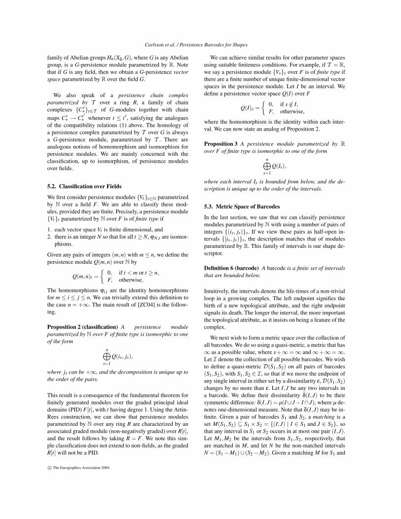
Example 13 (circle) In Example 6, we computed T filt(X)for a circle of radius R in the plane. We found that the entiretangent complex appeared when δ = 1/R. Below, we list thehomology groups, where we now use rows to delineate therange for δ. To reduce clutter, we omit the lower bound of δin each row, as it is implicitly defined by a higher row or iszero. We draw the corresponding barcodes in Figure 7.

δ 0 1< 1/R 0 0≥ 1/R F

2F

2

-

-

0 1R ∞

(a) β0

-

-

0 1R ∞

(b) β1

Figure 7: Barcodes for the circle.

Example 14 (ellipse) In Example 7, we computed T filt(X)

for the ellipse x2

a2 + y2

b2 = 1. While the full tangent complexT (X) matches that of the circle in the previous example, wesaw that Tδ(X) for the ellipse evolved through three stages,as shown in Figure 5. We draw the corresponding barcodesin Figure 8.

δ 0 1< a/b2 0 0< b/a2

F4 0

≥ b/a2F

2F

2

0 ab2

ba2

-

-

∞

(a) β0

0 ab2

ba2

-

-

∞

(b) β1

Figure 8: Barcodes for the ellipse.



7. Shape Recognition with Homology

In this section, we show how the homology of our tangentialconstructions is an effective tool for shape recognition andclassification. In particular, we see how the method can clas-sify objects in a continuous family of objects that have beenmodified by smooth deformations in the ambient space.

Example 15 (bottle vs. glass) In Example 5, we asked fora technique for distinguishing a bottle from a glass. The sur-faces are homeomorphic and share sharp features. Therefore,we must look at the filtered tangent complex for distinguish-ing features. In this example, we compute the barcode invari-ant for both objects and show how we may compare themusing our metric

Both a bottle and a glass may be described as surfaces ofrevolution, as shown in Figure 9. In both cases, we add a ver-tical line to the graph of a function. In order to study the fil-tered tangent complex, we need to make some assumptionsabout the shape of these objects. We begin with the bottle.Let f : [0,H]→R be a twice-differentiable positive functionwhose graph is used to sweep out a bottle of height H. Wemake the following assumptions about f and the principlecurvatures κrev and κgraph (cf. Example 8):

1. f is constant on the closed intervals [0,ξ0] and [ξH ,H],with f (0) > f (H), and is monotonically decreasing fromξ0 to ξH , with a single inflection point at ξ.

2. κrev is monotonically increasing.3. κgraph is 0 at the inflection point and the intervals where

f is constant, and has exactly two local maxima at ξ− ∈(ξ0,ξ) and ξ+ ∈ (ξ,ξH).

Let κ0 = κrev(0) = 1/ f (0) and κH = κrev(H) = 1/ f (H) de-note the inverse of the cross-sectional radii at 0,H, respec-tively. Clearly, κ0 < κH . Let κ− = κgraph(ξ−) and κ+ =κgraph(ξ+) denote the inverse of the radius of the osculat-ing circle to the curve at ξ−,ξ+, respectively. There are anumber of different cases for analyzing Tδ(X). We will dealwith the case 0 < κ+ < κ− < κ0 < κH , corresponding toa rather long, slowly tapering bottle, much like a Rieslingwine bottle. Other cases may be treated similarly. We obtainthe following results about Tδ(X).

• δ = 0: Any point where the curvature κgraph vanishes hasnon-empty fiber in T0(X). The projection of T0(X) decom-

(a) bottle (b) glass

Figure 9: Surfaces of revolution around the x-axis.

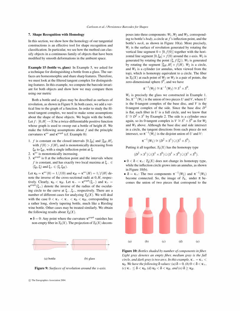
poses into three components: W1,W2 and W3, correspond-ing to bottle’s body, a circle at f ’s inflection point, and thebottle’s neck, as shown in Figure 10(a). More precisely,W1 is the surface of revolution generated by rotating thevertical line segment 0× [0, f (0)] together with the hori-zontal line segment [0,ξ0]× f (0) around the x-axis. W2 isgenerated by rotating the point (ξ, f (ξ)). W3 is generatedby rotating the segment [ξH ,H]× f (H). W2 is a circle,and W3 is a cylinder (or annulus, when viewed from thetop), which is homotopy equivalent to a circle. The fiberin T0(X) at each point of W2 or W3 is a pair of points, thezero-dimensional sphere S0, and we have

π−1(W2) ∼= π−1(W3) ∼= S1 ×S0.

W1 is precisely the glass we constructed in Example 1.So, π−1(W1) is the union of two pieces U and V , where Uis the 0-tangent complex of the base disc, and V is the0-tangent complex of the side. Since the base disc D2

is flat, each fiber in U is a full circle, and we know thatU ∼= D2 × S1 by Example 2. The side is a cylinder onceagain, so its 0-tangent complex is V ∼= S1 × S0 as for W2and W3 above. Although the base disc and side intersectin a circle, the tangent directions from each piece do notintersect, so π−1(W1) is the disjoint union of U and V :

π−1(W1) ∼= (D2 ×S1) ∪̇(S1 ×S0).

Putting it all together, T0(X) has the homotopy type

(D2 ×S1) ∪̇(S1 ×S0) ∪̇(S1 ×S0) ∪̇(S1 ×S0).

• 0 < δ < κ+: Tδ(X) does not change its homotopy type,while the inflection circle grows into an annulus, as shownin Figure 10(b).

• δ = κ+: The two components π−1(W2) and π−1(W3)become connected. So, the image of Tκ+ under π be-comes the union of two pieces that correspond to the

(a) (b) (c) (d) (e)

Figure 10: Bottles shaded by number of components in fiber.Light gray denotes an empty fiber, medium gray is the fullcircle, and dark gray is two arcs. In this example, κ− = κ+ <κ0. We have the following δ values: (a) δ = 0, (b) 0 < δ < κ+,(c) κ− ≤ δ < κ0, (d) κ0 < δ < κH , and (e) δ ≥ κH .



body and the neck. The fiber of any point away fromthe base disc is a pair of points or disjoint antipodal in-tervals. Along the crease of the base, the fiber is a dis-joint union of a circle and a pair of disjoint antipodal in-tervals. The complex description loses a term to becomeTκ+(X) ∼= (D2 ×S1) ∪̇(S1 ×S0) ∪̇(S1 ×S0).

• κ+ < δ < κ−: The homotopy type does not change.• δ = κ−: The neck and the body in the projection of Tδ(X)

merge, as shown in Figure 10(c). Every fiber is now non-empty, and consists of two antipodal arcs or points. Thehomotopy type of Tδ(X) loses another term to become(D2 ×S1) ∪̇(S1 ×S0).

• κ− < δ < κ0: The homotopy type does not change.• δ = κ0: Points along the lower sides of the bottle now

have full fiber. The individual fibers along the crease be-come a union of two circles, which now intersect in a pairof antipodal points. We now have

Tκ0(X) ∼= (D2 ×S1) ∪S1×S0 (S1 ×S1).

where ∪S1×S0 is the construction in Definition 1.• δ≥ κ0: The homotopy type remains unchanged, as shown

in Figures 10(d) and 10(e).

Our analysis gives the following description of homology forTδ(X).

δ 0 1 2< κ+ F

7F

7 0< κ− F

5F

5 0< κ0 F

3F

3 0≥ κ0 F F

3F

2

We next perform the same calculation for a glass shownin Figure 9(b). We assume it is the surface of revolution(0× [0,R])∪ ([0,H]×R) of radius R and height H. Observethat the glass is geometrically similar to the body of the bot-tle, the section called W1 when δ = 0 (or the surface in Ex-ample 1.) Let κ = 1/R. The analysis follows quickly fromour observation:

• δ = 0: We have T0(X) ∼= (D2 × S1) ∪̇(S1 × S0) as in theanalysis of π−1(W1) for the bottle.

• 0 < δ < κ: The homotopy does not change.• δ = κ: We have Tκ(X) ∼= (D2 × S1) ∪S1×S0 (S1 × S1) as

in the analysis for the bottle when δ = κ0.• δ > κ: The homotopy does not change.

Our analysis gives the following description of homology forTδ(X).

δ 0 1 2< κ F

3F

3 0≥ κ F F

3F

2

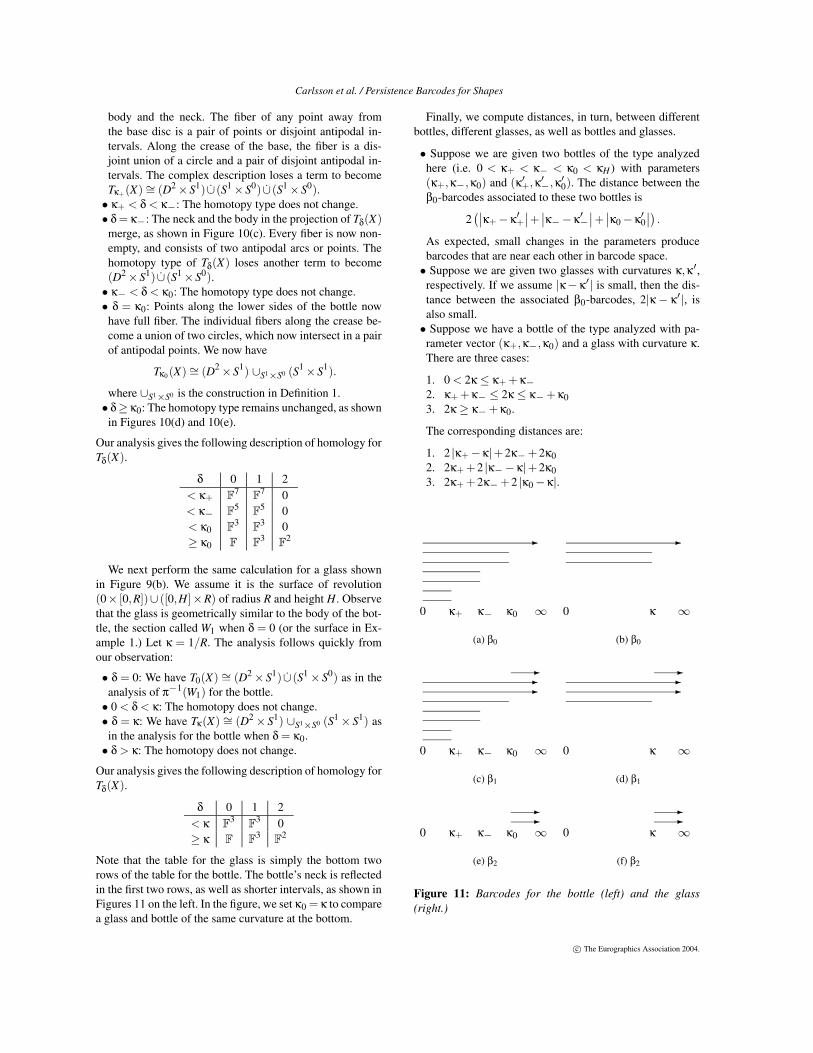
Note that the table for the glass is simply the bottom tworows of the table for the bottle. The bottle’s neck is reflectedin the first two rows, as well as shorter intervals, as shown inFigures 11 on the left. In the figure, we set κ0 = κ to comparea glass and bottle of the same curvature at the bottom.

Finally, we compute distances, in turn, between differentbottles, different glasses, as well as bottles and glasses.

• Suppose we are given two bottles of the type analyzedhere (i.e. 0 < κ+ < κ− < κ0 < κH ) with parameters(κ+,κ−,κ0) and (κ′

+,κ′−,κ′

0). The distance between theβ0-barcodes associated to these two bottles is

2(∣

∣κ+ −κ′+

∣

∣+∣

∣κ−−κ′−

∣

∣+∣

∣κ0 −κ′0∣

∣

)

.

As expected, small changes in the parameters producebarcodes that are near each other in barcode space.

• Suppose we are given two glasses with curvatures κ,κ′,respectively. If we assume |κ−κ′| is small, then the dis-tance between the associated β0-barcodes, 2|κ − κ′|, isalso small.

• Suppose we have a bottle of the type analyzed with pa-rameter vector (κ+,κ−,κ0) and a glass with curvature κ.There are three cases:

1. 0 < 2κ ≤ κ+ +κ−

2. κ+ +κ− ≤ 2κ ≤ κ− +κ03. 2κ ≥ κ− +κ0.

The corresponding distances are:

1. 2 |κ+ −κ|+2κ− +2κ02. 2κ+ +2 |κ−−κ|+2κ03. 2κ+ +2κ− +2 |κ0 −κ|.

0 κ+ κ− κ0 ∞

-

(a) β0

0 κ ∞

-

(b) β0

0 κ+ κ− κ0 ∞

-

-

-

(c) β1

0 κ ∞

-

-

-

(d) β1

0 κ+ κ− κ0 ∞-

-

(e) β2

0 κ ∞-

-

(f) β2

Figure 11: Barcodes for the bottle (left) and the glass(right.)



In the case of the bottle and the glass, the distances have di-mensions and are not relative, so we can reasonably expect agood performance from our distance function in distinguish-ing between the two. We can also visualize how changes inthe parameter values for the bottle will make it similar to aglass. As κ+,κ− tend to 0, we get longer and flatter bottles,arriving at a glass in the limit. We may observe the same ef-fect on the barcode, where the four shorter intervals becomeshorter as these parameters shrink, decreasing the bottle’sdistance to a glass.

8. Conclusion

In this paper, we propose a method for combining geometryand topology for shape recognition and classification. Ourmethod applies persistent homology to tangential construc-tions to arrive at a simple and compact shape descriptor, thebarcode, that captures both sharp and curvature-dependentfeatures of a shape. We also define a metric over the spaceof barcodes, and provide an algorithm for computing thismetric. Through detailed examples, we illustrate the viabil-ity of our method for shape recognition. In particular, weshow that we may think of our homologically invariant bar-codes as coordinates for shape spaces, as they lie in a metricspace. These coordinates correspond to geometric attributesof shapes, such as the eccentricity of an ellipse or the cur-vature of the neck of a bottle. They enable us to distinguishbetween interesting categories of shapes, such as betweenthe categories of bottles and glasses.

Our work suggestions major avenues for future research:

• Application of our techniques to point cloud data (PCD).There are a number of interesting computational questionsto be resolved, such as algorithms for constructing our de-rived complexes for the computation of barcodes. We havedone so for PCDs of curves [CZCG04]. We plan to applyour technqiues to PCDs of surfaces in the near future.

• Application of our techniques to noisy data. Our currentexperiments show that our techniques work well on ide-alized data, as well as data with superimposed Gaussiannoise.

• Development of statistical methods for analyzing data inthe metric space of barcodes. Such methods should per-mit the use of discriminant analysis and Bayesian deci-sion procedures to develop automatic methods for shapeclassification.

• Utilization of barcodes for coordinatizing spaces, for ex-ample, gray-scale images of families of three-dimensionalobjects.

• Utilization of linear algebraic algorithms recently devel-oped to locate features within data sets [CdS03].

We believe that the primary contribution of this paper is anapproach of blending geometric and topological techniquesthat is grounded in theory. As high throughput scanning be-comes commonplace, and more and more shapes are digi-tized, automatic qualitative shape analysis and classification

will be of critical value. Such analysis provides useful pri-ors for shapes that may be exploited for operations on them,such as reconstruction. We believe that the type of researchinitiated here will be important in the geometry processingfield in the years to come.

References

[BG92] BERGER M., GASTIAUX B.: Géomtrié dif-férentitelle: variétés, courbes et surfaces. Math-ématiques Presses Universitaires de France,Paris, France, 1992.

[Boo91] BOOKSTEIN F.: Morphometric Tools for Land-mark Data. Cambridge Univ. Press, Cambridge,UK, 1991.

[CdS03] CARLSSON G., DE SILVA V.: A geometricframework for sparse matrix problems. Ad-vances in Applied Mathematics (2003). (To ap-pear).

[CLRS01] CORMEN T. H., LEISERSON C. E., RIVEST

R. L., STEIN C.: Introduction to Algorithms.The MIT Press, Cambridge, MA, 2001.

[CZCG04] COLLINS A., ZOMORODIAN A., CARLSSON

G., GUIBAS L.: A barcode shape descriptor forcurve point cloud data, 2004. To appear in Proc.Symposium on Point-Based Graphics.

[DK90] DONALDSON S. K., KRONHEIMER P. B.: TheGeometry of Four-Manifolds. The ClarendonPress, New York, NY, 1990.

[ELZ02] EDELSBRUNNER H., LETSCHER D.,ZOMORODIAN A.: Topological persistenceand simplification. Discrete Comput. Geom. 28(2002), 511–533.

[Fan90] FAN T.-J.: Describing and Recognizing 3D Ob-jects Using Surface Properties. Springer-Verlag,New York, NY, 1990.

[Fed69] FEDERER H.: Geometric Measure Theory,vol. 153 of Die Grundlehren der Mathema-tischen Wissenschaften. Springer-Verlag, NewYork, NY, 1969.

[Fis89] FISHER R. B.: From Surfaces to Objects:Computer Vision and Three-Dimensional SceneAnalysis. John Wiley and Sons, Inc., New York,NY, 1989.

[GH81] GREENBERG M. J., HARPER J. R.: AlgebraicTopology: A First Course, vol. 58 of Mathemat-ics Lecture Note Series. Benjamin/CummingsPublishing Co., Reading, MA, 1981.

[GT89] GABOW H. N., TARJAN R. E.: Faster scalingalgorithm for network problems. SIAM J. Com-put. 18 (1989), 1013–1036.



[Hat01] HATCHER A.: Algebraic Topology. CambridgeUniv. Press, Cambridge, UK, 2001.

[KBCL99] KENDALL D., BARDEN D., CARNE T., LE H.:Shape and Shape Theory. John Wiley and Sons,Inc., New York, NY, 1999.

[Kuh55] KUHN H. W.: The Hungarian method for theassignment problem. Naval Research LogisticsQuarterly 2 (1955), 83–97.

[LPM01] LEE A. B., PEDERSEN K. S., MUMFORD

D.: The non-linear statistics of high contrastpatches in natural images. Tech. rep., BrownUniversity, 2001. Available online.

[Mil63] MILNOR J.: Morse Theory, vol. 51 of Annalsof Mathematical Studies. Princeton Univ. Press,Princeton, NJ, 1963.

[MS74] MILNOR J., STASHEFF J. D.: Characteris-tic Classes, vol. 76 of Annals of MathematicalStudies. Princeton Univ. Press, Princeton, NJ,1974.

[ZC04] ZOMORODIAN A., CARLSSON G.: Comput-ing topological persistence, 2004. To appear inProc. 20th Ann. ACM Sympos. Comput. Geom.

[ZY96] ZHU S., YUILLE A.: Forms: A flexible objectrecognition and modeling system. Int. J. Comp.Vision 20, 3 (1996), 187–212.


Documents

Persistence Barcodes for Shapes