PERUVIAN ECONOMIC ASSOCIATION Peru’s Great …perueconomics.org/wp-content/uploads/2014/01/WP-45.pdf1 Peru's Great Depression A Perfect Storm? Gonzalo Llosa and Ugo Panizza * The

PERUVIAN ECONOMIC ASSOCIATION

Peru’s Great Depression A Perfect Storm?

Luis Gonzalo Llosa

Ugo Panizza

Working Paper No. 45, May 2015

The views expressed in this working paper are those of the author(s) and not those of the Peruvian

Economic Association. The association itself takes no institutional policy positions.

1

Peru's Great Depression

A Perfect Storm?

Gonzalo Llosa and Ugo Panizza

*

The expression “Perfect Storm” refers to the simultaneous occurrence of events

which, taken individually, would be far less powerful than the result of their

combination. Such occurrences are rare by their very nature, so that even a slight

change in any one event contributing to the perfect storm would lessen its overall

impact. (Wikipedia)

Introduction

Over the 1970s and 1980s Peru went through a series of deep and protracted

economic crises which generated enormous output losses. While output collapses are

not uncommon in the emerging world (in a sample of 31 emerging market countries

over the 1980-2004 period, Calvo et al., 2006 identify 22 events), Peru stands apart

for the rapid succession of crises. For three times in a row, as soon as output would

recover to its pre-crisis level, a new crisis would hit the country and destroy all the

progress made during the previous years. As a consequence, the growth rate of Peru's

GDP per capita averaged to 0 percent over a thirty-year period (1975-2005), a horrible

performance even when compared to Latin America's dismal rate of economic

growth. Moreover, while Calvo et al. (2006) document that great depressions tend to

be V-shaped (i.e., characterized by a rapid collapse and a rapid recovery with almost

no investment), the recovery from Peru's deepest collapse took 15 years, clearly not a

V-shaped crisis.

The objective of this paper is to describe Peru's great depression and discuss

possible hypotheses that may explain the deep collapse and slow recovery of the

Peruvian economy. The main finding of the paper is that it is very hard to find a single

explanation for Peru's great depression. Very much like a perfect storm, so many

things went wrong at the same time, with the effects of each negative shock

amplifying those of the other shocks. In particular, our findings suggest that the

external shocks that hit the country in the 1980s were amplified by a weak and

* Llosa is with the Research Department of the Inter American Development Bank and Panizza with

the Debt and Finance Analysis Unit of the Division of Globalization and Development Strategies of

UNCTAD. We would like to thank Miguel Castilla, Jeff Frieden, Ricardo Hausmann, Eduardo Moron,

Francisco Rodriguez and seminar participants at Harvard's JFK School for useful comments and

suggestions. The opinion expressed in this paper are those of the authors and do not necessarily reflect

those of the Inter-American Development Bank or UNCTAD. The usual caveats apply.

2

fractionalized political system (for a discussion of the interaction between external

shocks and ability to recovery from external shocks, see Rodrik, 1999), limited

domestic entrepreneurial capacity, and lack of a coherent industrial policy that could

lead to the discovery of new productive activities.

The Lost Three Decades

A deep regional economic crisis led the UN Economic Commission for Latin America

(ECLAC) to call the 1980s the continent's "lost decade". While the 1980s were not a

happy period for Latin America, they were a disastrous one for Peru. Figure 1 shows

that, starting 1975, Peru faced a series of economic crises and an enormous output

contraction. If Latin America lost one decade, Peru lost three decades.

The objective of this section is to provide an anatomy of Peru's growth

collapse. The main message of the section is that not only was the depth of Peru's

recession unusually large, but its recovery was unusually slow. Hence, one of the

main challenges in understanding Peru's growth performance is explaining the reason

for this slow recovery.

In order to move beyond the simple graphical analysis of Figure 1 and analyze

if there was something special about the collapse and recovery in Peru's GDP growth,

we need to be able to compare Peru with other countries which also had serious

economic troubles. In order to do so, we identify growth contractions in a large

sample of countries and then compare Peru with other countries that went through

growth contractions.

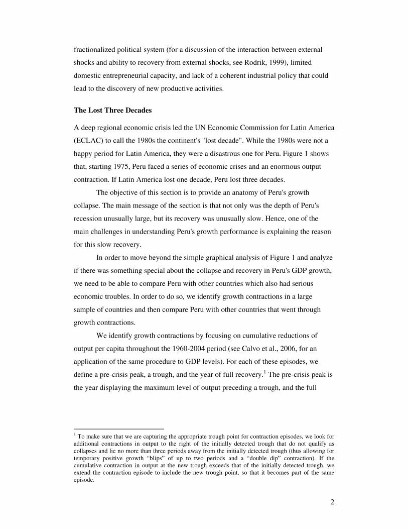
We identify growth contractions by focusing on cumulative reductions of

output per capita throughout the 1960-2004 period (see Calvo et al., 2006, for an

application of the same procedure to GDP levels). For each of these episodes, we

define a pre-crisis peak, a trough, and the year of full recovery.1 The pre-crisis peak is

the year displaying the maximum level of output preceding a trough, and the full

1 To make sure that we are capturing the appropriate trough point for contraction episodes, we look for

additional contractions in output to the right of the initially detected trough that do not qualify as

collapses and lie no more than three periods away from the initially detected trough (thus allowing for

temporary positive growth “blips” of up to two periods and a “double dip” contraction). If the

cumulative contraction in output at the new trough exceeds that of the initially detected trough, we

extend the contraction episode to include the new trough point, so that it becomes part of the same

episode.

3

recovery point is the year in which the pre-crisis peak output level is fully restored.2 A

trough is the local minimum following the onset of a crisis. We identify 782 episodes,

of which 155 are in Latin America and 4 in Peru, indicating that Peru did not have

more contractions than the average Latin America country (the regional average is 5

collapses). However, by focusing only on those episodes with a cumulative

contraction bigger than 5 percent of GDP, we find that Peru experienced more

contractions than the average Latin American country.

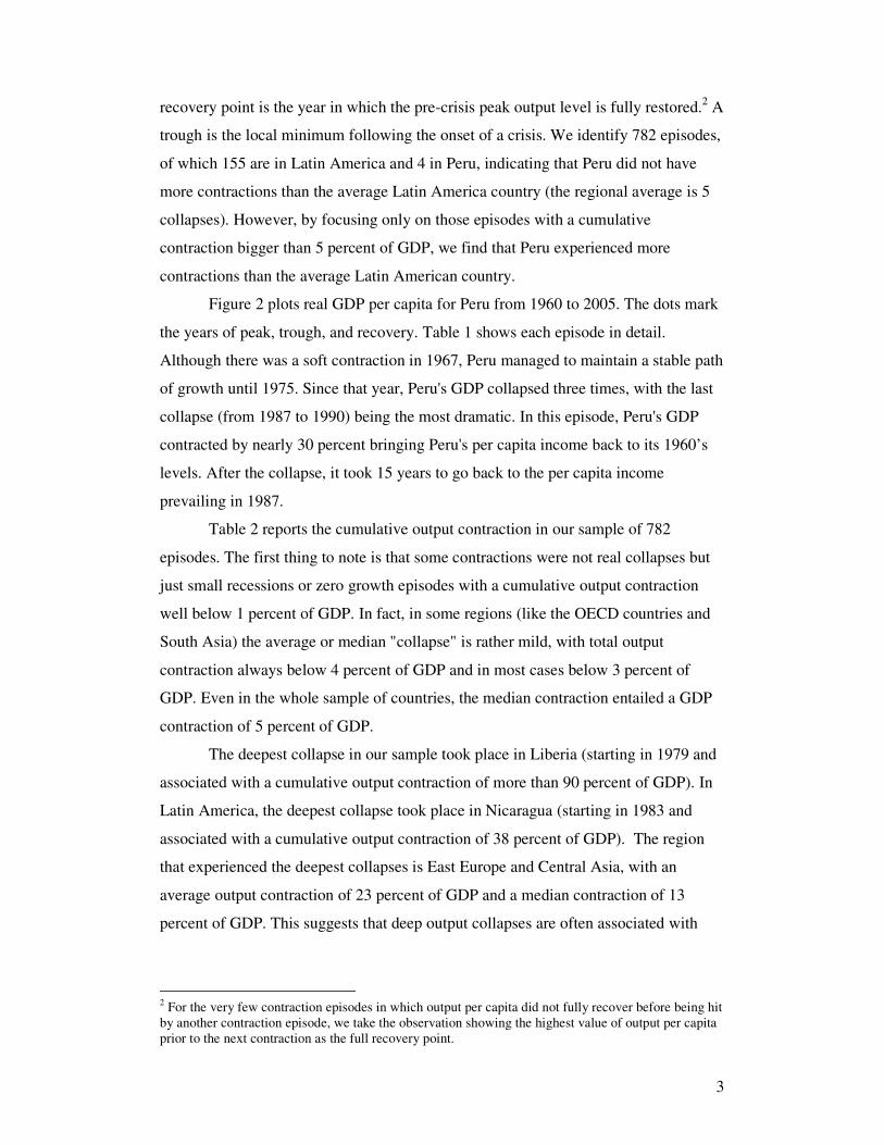
Figure 2 plots real GDP per capita for Peru from 1960 to 2005. The dots mark

the years of peak, trough, and recovery. Table 1 shows each episode in detail.

Although there was a soft contraction in 1967, Peru managed to maintain a stable path

of growth until 1975. Since that year, Peru's GDP collapsed three times, with the last

collapse (from 1987 to 1990) being the most dramatic. In this episode, Peru's GDP

contracted by nearly 30 percent bringing Peru's per capita income back to its 1960’s

levels. After the collapse, it took 15 years to go back to the per capita income

prevailing in 1987.

Table 2 reports the cumulative output contraction in our sample of 782

episodes. The first thing to note is that some contractions were not real collapses but

just small recessions or zero growth episodes with a cumulative output contraction

well below 1 percent of GDP. In fact, in some regions (like the OECD countries and

South Asia) the average or median "collapse" is rather mild, with total output

contraction always below 4 percent of GDP and in most cases below 3 percent of

GDP. Even in the whole sample of countries, the median contraction entailed a GDP

contraction of 5 percent of GDP.

The deepest collapse in our sample took place in Liberia (starting in 1979 and

associated with a cumulative output contraction of more than 90 percent of GDP). In

Latin America, the deepest collapse took place in Nicaragua (starting in 1983 and

associated with a cumulative output contraction of 38 percent of GDP). The region

that experienced the deepest collapses is East Europe and Central Asia, with an

average output contraction of 23 percent of GDP and a median contraction of 13

percent of GDP. This suggests that deep output collapses are often associated with

2 For the very few contraction episodes in which output per capita did not fully recover before being hit

by another contraction episode, we take the observation showing the highest value of output per capita

prior to the next contraction as the full recovery point.

4

civil wars or with dramatic changes in a country's economic structure (like the

transition from plan to market).

The data of Table 2 provide a first indication of the seriousness of Peru's 1981

and 1987 growth collapses. The output contraction that started in 1981 entailed an

output loss which was twice the cross-country average and three times the cross-

country median, and this was only the second most severe contraction for Peru. The

output loss of the contraction that started in 1987 was three times the cross-country

average and more than 5 times the cross-country median. In fact, the Peruvian

contraction of 1987 is comparable to contractions taking place during episodes of civil

war or economic transition.

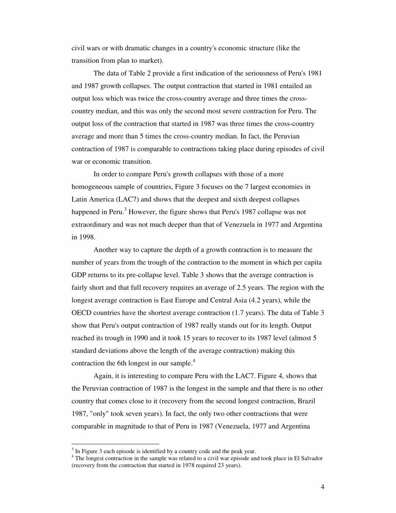
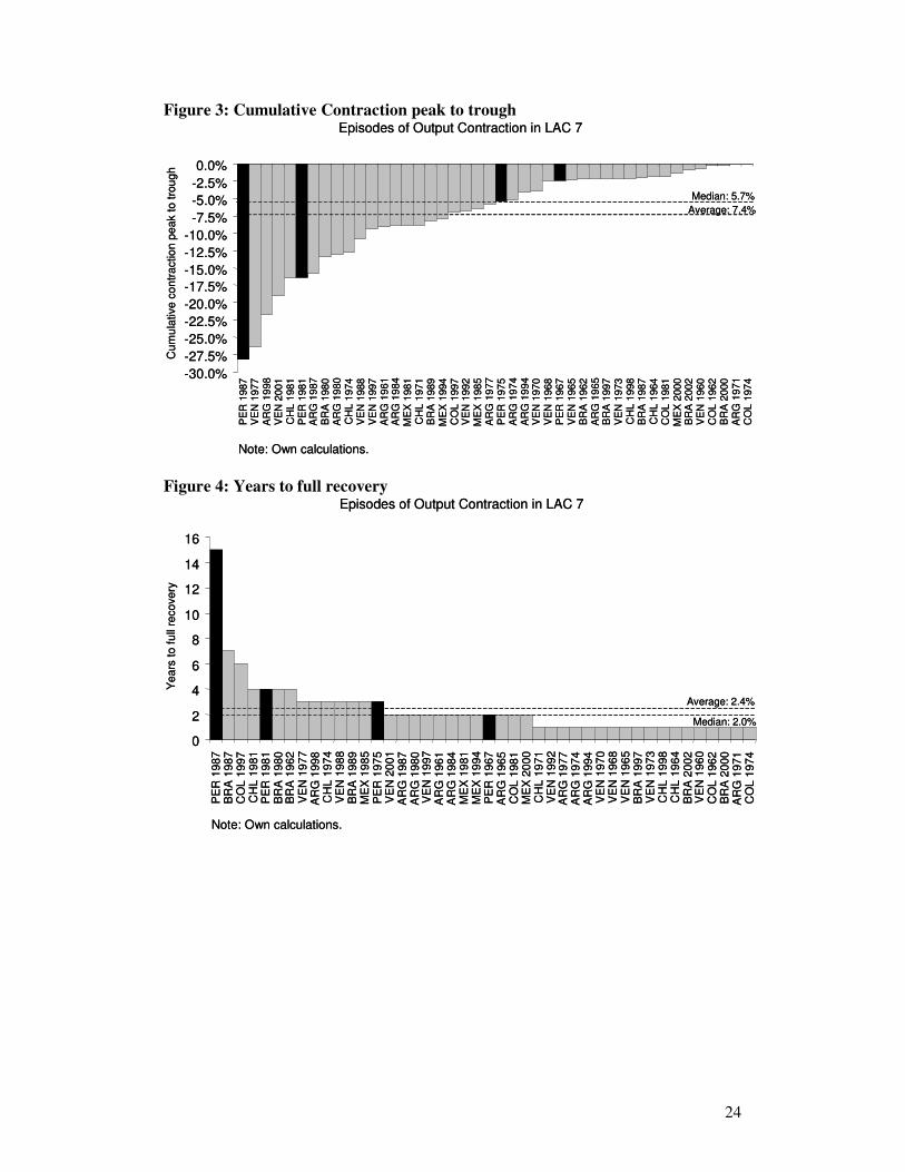
In order to compare Peru's growth collapses with those of a more

homogeneous sample of countries, Figure 3 focuses on the 7 largest economies in

Latin America (LAC7) and shows that the deepest and sixth deepest collapses

happened in Peru.3 However, the figure shows that Peru's 1987 collapse was not

extraordinary and was not much deeper than that of Venezuela in 1977 and Argentina

in 1998.

Another way to capture the depth of a growth contraction is to measure the

number of years from the trough of the contraction to the moment in which per capita

GDP returns to its pre-collapse level. Table 3 shows that the average contraction is

fairly short and that full recovery requires an average of 2.5 years. The region with the

longest average contraction is East Europe and Central Asia (4.2 years), while the

OECD countries have the shortest average contraction (1.7 years). The data of Table 3

show that Peru's output contraction of 1987 really stands out for its length. Output

reached its trough in 1990 and it took 15 years to recover to its 1987 level (almost 5

standard deviations above the length of the average contraction) making this

contraction the 6th longest in our sample.4

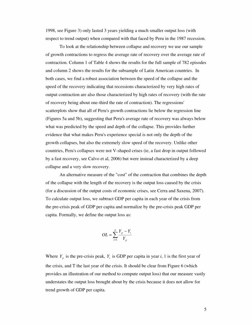
Again, it is interesting to compare Peru with the LAC7. Figure 4, shows that

the Peruvian contraction of 1987 is the longest in the sample and that there is no other

country that comes close to it (recovery from the second longest contraction, Brazil

1987, "only" took seven years). In fact, the only two other contractions that were

comparable in magnitude to that of Peru in 1987 (Venezuela, 1977 and Argentina

3 In Figure 3 each episode is identified by a country code and the peak year.

4 The longest contraction in the sample was related to a civil war episode and took place in El Salvador

(recovery from the contraction that started in 1978 required 23 years).

5

1998, see Figure 3) only lasted 3 years yielding a much smaller output loss (with

respect to trend output) when compared with that faced by Peru in the 1987 recession.

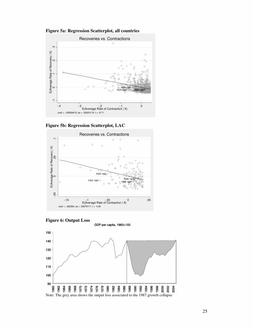
To look at the relationship between collapse and recovery we use our sample

of growth contractions to regress the average rate of recovery over the average rate of

contraction. Column 1 of Table 4 shows the results for the full sample of 782 episodes

and column 2 shows the results for the subsample of Latin American countries. In

both cases, we find a robust association between the speed of the collapse and the

speed of the recovery indicating that recessions characterized by very high rates of

output contraction are also those characterized by high rates of recovery (with the rate

of recovery being about one-third the rate of contraction). The regressions'

scatterplots show that all of Peru's growth contractions lie below the regression line

(Figures 5a and 5b), suggesting that Peru's average rate of recovery was always below

what was predicted by the speed and depth of the collapse. This provides further

evidence that what makes Peru's experience special is not only the depth of the

growth collapses, but also the extremely slow speed of the recovery. Unlike other

countries, Peru's collapses were not V-shaped crises (ie, a fast drop in output followed

by a fast recovery, see Calvo et al, 2006) but were instead characterized by a deep

collapse and a very slow recovery.

An alternative measure of the "cost" of the contraction that combines the depth

of the collapse with the length of the recovery is the output loss caused by the crisis

(for a discussion of the output costs of economic crises, see Cerra and Saxena, 2007).

To calculate output loss, we subtract GDP per capita in each year of the crisis from

the pre-crisis peak of GDP per capita and normalize by the pre-crisis peak GDP per

capita. Formally, we define the output loss as:

∑=

−=

T

i p

ip

Y

YYOL

1

Where pY is the pre-crisis peak, iY is GDP per capita in year i, 1 is the first year of

the crisis, and T the last year of the crisis. It should be clear from Figure 6 (which

provides an illustration of our method to compute output loss) that our measure vastly

understates the output loss brought about by the crisis because it does not allow for

trend growth of GDP per capita.

6

Table 5 shows that the 1987 crisis led to an output loss equal to almost three

times the pre-crisis GDP per capita. Figure 7 shows that Peru's output loss was by far

the largest in Latin America, almost 50 percent larger than the second deepest output

loss (Venezuela in 1977) and 5 times the third deepest output loss (Argentina in

1989).

Trying to Explain Peru's Growth Performance

What can explain Peru's dismal growth performance? Our working hypothesis is that

Peru was hit by a perfect storm with mutual reinforcing negative effects of external

shocks, political instability, and limited domestic entrepreneurship and ability to

develop new export activities. In this section, we will explore the interaction of these

factors and highlight how each of them played a key role in Peru's growth collapse.

Before doing so, it is worth painting a brief picture of the Peruvian economy in the

mid 1970s.

The Peruvian Economy in the 1970s

Peru was never a fast growing country. According to Thorp and Bertram's (1978)

authoritative economic history, over the 1890-1970 period, Peru’s GDP per capita

grew at an average rate of 1 percent per year. Moreover, growth was concentrated in

the coastal region and completely driven by the export of primary products

(agriculture, fishing, and mining). High revenues from natural resources led to Dutch

disease and seriously limited Peru's ability to develop a national industry both for

import substitution and export of manufacturing. In fact, the small manufacturing

sector was dominated by activities related to the processing of export products and,

like most of the extractive industry, often under the control of foreign investors.

Moreover, the constant overvaluation of the exchange rate reduced the viability of

subsistence farming (which could not compete with imported products) and further

increased the geographical fragmentation of economic growth in Peru.

Attempts to create a local industry were not successful. One of such attempts

was the industrial promotion law of 1959 which gave incentives for investment in

industry (mainly through exemption from import duties on equipment and

intermediate goods and by not taxing reinvested profits). However, the law was too

7

generous and not selective. While most countries that were implementing similar

industrial promotion laws restricted incentives to new activities, the Peruvian law did

not discriminate across sectors and ended up benefiting export processing activities

and slow-growing industries (like the textile). In fact, since the law made no attempt

at promoting domestic entrepreneurial capacity it ended up benefiting FDIs in export

processing industries.

The concentration of economic activity in few capital-intensive sectors and

specific geographical areas led to increasing income inequality which, in turn, led to

political fragmentation. The consequence (and to some instance, the cause) of foreign

ownership of most productive activities was a limited domestic entrepreneurial

capacity. As we will see below, both of these factors played an important role in

Peru's growth collapse and slow recovery.

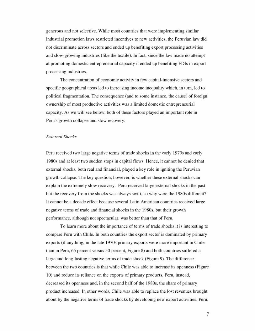
External Shocks

Peru received two large negative terms of trade shocks in the early 1970s and early

1980s and at least two sudden stops in capital flows. Hence, it cannot be denied that

external shocks, both real and financial, played a key role in igniting the Peruvian

growth collapse. The key question, however, is whether these external shocks can

explain the extremely slow recovery. Peru received large external shocks in the past

but the recovery from the shocks was always swift, so why were the 1980s different?

It cannot be a decade effect because several Latin American countries received large

negative terms of trade and financial shocks in the 1980s, but their growth

performance, although not spectacular, was better than that of Peru.

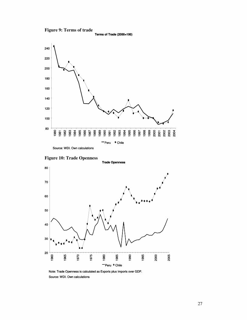
To learn more about the importance of terms of trade shocks it is interesting to

compare Peru with Chile. In both countries the export sector is dominated by primary

exports (if anything, in the late 1970s primary exports were more important in Chile

than in Peru, 65 percent versus 50 percent, Figure 8) and both countries suffered a

large and long-lasting negative terms of trade shock (Figure 9). The difference

between the two countries is that while Chile was able to increase its openness (Figure

10) and reduce its reliance on the exports of primary products, Peru, instead,

decreased its openness and, in the second half of the 1980s, the share of primary

product increased. In other words, Chile was able to replace the lost revenues brought

about by the negative terms of trade shocks by developing new export activities. Peru,

8

on the contrary, did not develop new export activities, openness decreased and, if

anything the negative terms of trade shock increased the importance of primary

exports in total exports.

An alternative way to look at the impact of the negative terms of trade shock

on Peru's growth performance is to estimate how terms of trade shock affect output

collapses and test whether there is something special about the Peruvian experience.

In Table 6 we focus on our sample of growth contractions and regress the size of the

output contraction over the change in terms of trade (measured as the difference

between peak and trough). As expected, we find that the terms of trade variable has a

positive coefficient, indicating that larger negative terms of trade shocks are

associated with deeper contractions. Figure 11 plots the relationship between the

terms of trade shock and output contraction (the figure is based on column 2 of Table

6, figures based on other regressions yield similar results) and show that Peru's output

contractions of 1981 and 1987 were much deeper than what was predicted by the

terms of trade shock. This provides additional evidence that, while negative terms of

trade shocks may have played a role in igniting Peru's great depression, they cannot

fully explain the dept of the collapses; something else must have gone wrong.5

Bad Economic Policies

Another explanation for Peru's growth collapse focuses on disastrous and inconsistent

macroeconomic policies.6 Macroeconomic mismanagement is clearly illustrated by a

history of high inflation (in the 1970s and early 1980s) that culminated in

hyperinflation in the late 1980s and by an extremely poor fiscal performance (Figure

12 shows that over the 1978-2004 period Peru's budget deficits have always been

larger than the Latin American average). Bottlenecks caused by insufficient public

investment in infrastructure can also be part of the story. Figure 13 shows that in Peru

investment in infrastructure was well below the LAC6 average and that the difference

was particularly large in the second half in the 1980s.

However, while on average Latin America had better fiscal results than Peru,

it is difficult to establish a causal relationship going from deficit to GDP growth. It is,

5 We obtain similar results when we use terms of trade shocks to explain the size of the output loss.

6 Bad microeconomic policies also played a role. See, for instance, Thorp and Bertram’s (1978)

discussion of Peru’s industrial policy and Jenkner’s (2006) analysis of the link between reforms and

growth in Peru.

9

in fact, plausible that the poor fiscal results were partly driven by low tax revenues

associated with low economic growth. Similarly, while the collapse in investment in

infrastructure is certainly part of the story, it cannot be the whole story since it

happened after and not before the crisis. A plausible interpretation is that the

economic crisis tightened the government budget constraint and this led to a

contraction in investment in infrastructure. While this may have served has an

amplifying factor, it cannot be the only explanation for such a protracted crisis.

An alternative explanation focuses on the fact that not only macroeconomic

policies were often irresponsible, but that even responsible policies tended to be

unpredictable and characterized by frequent swings of the pendulum (Carranza et al,

2005). This interpretation is consistent with the lack of a clear correlation between the

policy stance of a given administration and economic performance. In fact, Figure 14

shows that Peru did poorly under very different types of economic policy. Peru's

growth performance started deviating from the Latin American average during a

period in which the administration of President Velasco adopted a set of isolationist

economic policies, but divergence continued when the administration of President

Belaunde adopted more market-oriented policies, and further expanded with the

heterodox experiment of President Garcia. GDP growth picked up with the pro-

market policies adopted by President Fujimori and per capita income grew by 10

percent in 1994 and 6 percent in 1995. However, during 1995-2005 GDP growth

averaged to a more modest 1.6 percent, preventing Peru from catching up with the rest

of Latin America.

While there is truth in the fact that poor macroeconomic management

amplified the external shocks that hit the country in the late 1970s, these poor

macroeconomic policies were partly endogenous to the crisis. A plausible story is

that the correction of the large external shocks would have required a set of unpopular

adjustment policies, but the high degree of political fragmentation (partly driven by

rising inequality) did not allow reaching the national consensus necessary to adopt

such policies. So, a vicious circle with a continuous feedback between low (or

negative) growth and policy instability (for a detailed discussion of this mechanism,

see Rodrik, 1999) clearly played a key role in explaining Peru’s lost three decades.

Yet, one feels that part of the explanation is still missing. After all, several Latin

American countries characterized by high inequality and fractionalized political

systems faced external shocks similar to those that hit Peru, but they “only” lost one

10

decade. Why did Peru lose three? Why was the recovery so slow? We suspect that the

third element of Peru’s perfect storm is that Peru was unable to develop new

manufacturing capacity that would replace the traditional export sectors hit by the

negative external shocks. It is worth noting that this hypothesis is in line with Thorp

and Bertram’s (1978) interpretation of Peru’s growth experience:

"…local capacity to innovate and adapt technology; endogenous as

distinct from external sources of economic dynamism; and policies which

foster integrated growth….might have permitted the economy to survive

the periodic breakdown of the export mechanism without high cost in

terms of growth….It would also have prepared the economy more

successfully to tackle the increasingly large scale and more complex

investment projects required to sustain growth in the export sector.

(Thorp and Bertram, 1978, pp 321-322)

Although we cannot provide a direct test of the above hypothesis, it is possible

to use industry-level data to explore what might have constrained the growth of Peru’s

manufacturing sector. This is what we do in the next section.

Obstacle to Manufacturing Growth: A Sector-Level Analysis

While previous studies looked at the determinants of Peru's growth performance by

using cross-country or time series data (eg. Carranza et al., 2005 and Jenkner, 2006),

we focus on the evolution of different sectors within the Peruvian economy.

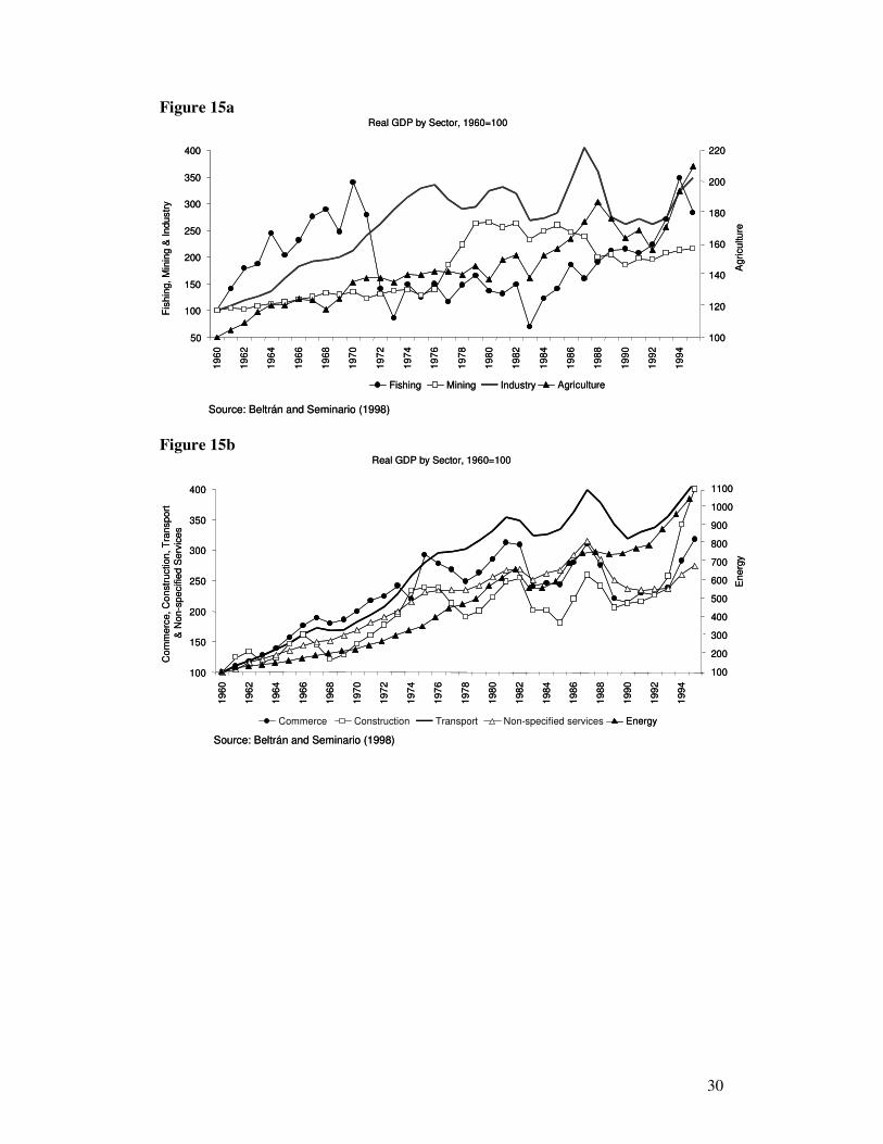
Figures 15a and 15b show that there is substantial heterogeneity across

sectors. First of all, there was no collapse in the transport and energy sectors which

kept growing throughout the 1970s and 1980s. Agriculture did not collapse in the

1970s, but it was already stagnating from before.7 The fishing sector was the first to

collapse (due to overexploitation, Bertram and Thorp 1978) in the early 1970s. It

recovered in the late 1980s but fish production did not reach the level of 1970; until

1994. The mid 1970s mark the collapse of commerce, construction, other services,

and industry.

Given the fact that most of Peru’s industrial production was linked to the

processing of primary products, it is not hard to explain why the collapse of the

fishing industry and the mining sector had a negative impact on industrial production.

7 A possible interpretation for this lackluster performance was the climate of uncertainty caused by

early proposals (dating back to the 1960s) of agricultural reforms (Bertram and Thorp, 1978).

11

What is more difficult to explain is why it took Peru so long to develop new

industries. To shed some light on this issue, we use UNIDO data on value added to

explore in greater details the behavior of Peru's industrial sectors. To maximize the

country coverage we focus on the 1974-1996 period.8 In order to limit country

heterogeneity, we will not compare the performance of Peru with that of the industrial

countries or with that of Africa, but limit our analysis to Latin America and emerging

Asia. These are two groups of countries which in the 1970s had similar levels of per

capita income but, since then, had very different growth performances.

Figure 16 shows that, on average, the annual growth rate of Peru's industrial

sectors was 5 percentage points lower than that of the rest of Latin America. There

are, however, large differences across sectors. For instance, the Peruvian oil-refining

sector grew faster than the Latin American average, but in Peru the growth rate of

pottery and other manufacturing products was ten percentage points below the

regional average. Figure 17 compares Peru with East Asia. In this case, we find that

the growth rate of Peru's industrial sectors was five percentage points lower than that

of East Asia. Again, we find large differences across sectors with Peru leading in the

oil refining sector but lagging in machinery, chemicals, pottery and other industrial

products.

Why did some sectors perform much worse than others? We explore three

possible answers: (i) lack of financing; (ii) problems with the labor market; and (iii)

problems with the export sector.

Lack of Financing

There is substantial research showing the existence of a causal relationship going

from access to finance to growth (for a survey see Levine, 2004 and for an application

to Peru see the chapter by Braun and Serra in this volume). As the size of the

Peruvian credit market is extremely small (see the Chapter by Braun and Serra for

further discussion) it is tempting to think that the small financial system is one of the

key culprits in Peru's poor growth performance. We can test this hypothesis by

checking whether the industrial sectors that did relatively worse in Peru are those

sectors that need a larger access to external financial sources:

8 This period works well for Peru, since 1974 marks the beginning of the growth collapse while 1996

the end of the mini-recovery that followed the election of President Fujimori.

12

tjiiijtitji PERULACEXFINVAGR ,,,,, )**(* εργβα ++++= (1)

Where VAGR measures value added growth in country i, sector j, year t. ti,α is a

country-year fixed effect that captures all shocks that are country-year specific (thus,

it captures all macroeconomic factors like inflation, GDP growth, capital flows,

exchange rate, etc). EXFIN is the Rajan and Zingales (1998) measure of firms'

demand for external finance (in order to compare the effect of external finance with

other variables that will be introduced below, we standardize EXFIN so that its mean

is equal to zero and its standard deviation equal to one). LAC is a dummy variable

taking value one for countries in Latin America and zero otherwise, and PERU is a

dummy variable taking value one for Peru and zero otherwise. Since the sample only

includes Latin America and East Asia, the coefficient β measures whether East

Asian firms that demand more external financing grew at a faster rate than firms that

can finance themselves using internal resources. The sum of β and γ provides the

same information for firms located in Latin America (excluding Peru) and β +γ + ρ

measures how demand for external finance affects firm growth in Peru. Hence, the

coefficient ρ measures whether sectors which are relatively more dependent on

external finance did worse in Peru than in the rest of Latin America (γ + ρ provides a

similar comparison with East Asia).

If we were to find that ρ is negative and large, then we could conclude that

sectors that require a lot of external finance did relatively poorly in Peru. This fact

would be consistent with the idea that the small size of the Peruvian financial market

played a key role in the poor growth performance of the Peruvian economy. The first

four columns of Table 7 present the results. Column 1 uses the whole sample (going

from 1974 to 1996) and shows that β is positive and large (a one standard deviation

increase in the demand of external finance is associated with a 1.5 percentage points

in annual value added growth). The coefficient interacted with the Latin American

dummy (γ ) is instead negative and statistically significant. This indicates that in

Latin America, firms that need more access to external finance do relatively worse

than similar firms located in East Asia and that lack of access to finance may be part

of the explanation of why growth in Latin America has been slower than in East Asia.

13

More interestingly, we find that ρ is positive and statistically significant. This

indicates that Peruvian firms that need more external financing do relatively better

than similar firms located in the rest of Latin America. Hence, lack of access to

finance cannot explain the differences in sectoral performance documented in Figure

16. Furthermore, the fact that 0≈+ ργ suggests that there is no difference in the

relative performance of Peruvian and East Asian firms which need more external

finance. Again, this suggests that the underdevelopment of the Peruvian financial

market cannot be an explanation for the sectoral differences in value added growth

documented in Figure 16.

Columns 2-4 of Table 7 split the sample into 3 sub-periods: 1974-1979

(column 2), 1980-1989 (column 3), and 1990-1996 (column 4). They show that lack

of access to finance was not a determinant of low growth in the 1970s and 1980s.

However, column 4 shows that over 1990-1996 Peruvian industries with larger needs

of external finance grew at a significantly slower rate with respect to similar firms

located in the rest of Latin America and in East Asia (the difference in annual value

added growth was 2 and 3.4 percentage points, respectively). Therefore, lack of

access to finance may explain the lack of convergence in the 1990s, but not what

happened in the 1980s.

We obtain similar results when we estimate the following regression which

allows looking separately at the largest Latin American economies:

tjiiijtitji PERUOTHLALAEXFINVAGR ,,,,, )**6*(* ερλγβα +++++= (2)

Where LA6 is a dummy variable that takes value one for Argentina, Brazil, Chile,

Colombia, Mexico, and Venezuela (together with Peru, these are the largest Latin

American economies) and zero otherwise. OTHLA takes value one for all Latin

American countries with the exclusion of the counties included in LA6 and Peru. All

the other variables are defined as above. In this case the coefficients should be

interpreted as follows: ρ measures whether sectors which are relatively more

dependent on external finance did relatively worse (a negative sign) or better (a

positive sign) in Peru than in East Asia; γ and λ instead compare East Asia with the

LA6 countries and the other Latin American countries, respectively. When we focus

on the whole period (column 5), we find no difference between Peru and Latin

14

America. Focusing on the 1970s and 1980s, we find that Peruvian firms with more

needs of external finance did better than similar firms located in East Asia. However,

the opposite is true in the 1990s. This confirms that lack of access to finance may be

an explanation for the relatively low growth of the early 1990s, but is unlikely to

explain the disastrous outcomes of the 1970s and 1980s.

Problems with the labor market

Labor laws implemented during the early 1970s and the mid 1980s made the Peruvian

labor market extremely rigid. In Saavedra and Torero’s (2004, page 131) words: "the

Peruvian Labor Code developed during the import substitutions period had been

termed one of the most restrictive, protectionist and cumbersome in Latin America."

We can use a strategy similar to the one described above to test if the lack of a

well-working labor market played a role in explaining Peru's growth performance. In

particular, we start by computing a measure of labor intensity at the country-industry-

level and then use this measure to test whether more labor intensive industries did

particularly poorly in Peru relative to similar industries in the rest of Latin America

and East Asia.9 Here, we have an interesting experiment because a series of reforms

implemented in the early 1990s led to a substantial deregulation of the Peruvian labor

market. If labor regulation was the main obstacle to Peruvian growth, we should

observe that labor-intensive industries recovered in the 1990s.

We report our main results in Table 8 (the econometric specifications used in

this table are identical to those used in Table 7, but we now substitute EXFIN with

LI). Column 1 focuses on the whole period and finds that ρ has a negative coefficient

which is both statistically and economically significant. This indicates that, during the

period under observation, labor intensive industries located in Peru grew relatively

slower than similar industries located in the rest of Latin America or East Asia (there

are no significant differences between the Latin American average and those of East

9 We measure labor intensity by dividing value added by the number of employees and then compute

an average across the period. Formally, labor intensity in country i industry j is defined as:

∑=

=1996

1974 ,,

,,

,22

1

t tji

tji

jiEMP

VALI . As in the case of EXFIN, we standardize LI so that its mean is zero and

its standard deviation is one.

15

Asia). The problem is that the coefficient is highly unstable across periods. It is large

and positive in the 1970s (column 2 of Table 8) and negative in the 1980s and 1990s

(statistically significant only in the 1980s). While the negative coefficient of the

1980s is consistent with the tightening of the labor laws implemented by the

administration of President Garcia, the fact that we also find a negative coefficient

also in the 1990s (a period of labor market deregulation) is more puzzling. The last

four columns of Table 8 split the Latin American coefficient using an empirical

strategy identical to that described in Equation (2) and corroborate the results of the

first four columns.

Problems with the export sector

As the experience of several East Asian economies has shown that the export sector

can be an important source of economic growth, we explore the hypothesis that the

root of Peru's slow recovery had something to do with a crisis of the export sector.

There are several events that may have damaged the Peruvian export sector. The first

had to do with the isolationist policy stance adopted in the late 1960s by the

administration of president Velasco (according to Bertram and Thorp, 1978, until the

mid 1960s Peru had one of the most outward-oriented economic policies in Latin

America). The second relates to Dutch disease and the extreme volatility of Peru's real

exchange rate (Frankel and Wei, 1998 show that a one percent increase in the

volatility of the bilateral exchange rate reduces trade by as much as 1.8 percent).10

The third explanation relates to the fact that the non-selective industrial policy

described above did not provide the incentives to discover new export activities that

could replace the traditional export industries.11

Again, we can check whether there were problems in the export sectors by

estimating regressions similar to those of Equations 1 and 2 and substituting the

industry-level measure of financial dependence with an industry-level measure of

10

We computed the standard deviation of the bilateral (vis a vis the USD) real exchange rate for all

countries for which we had data for the 1974-1990 period. The average standard deviation for the 102

countries in our sample was 0.18 and the median value was 0.16. The value for Peru was 0.36. This

puts Peru in the top 5th

percentile of the distribution. The only 4 countries where volatility was higher

than Peru are: Zaire, Chile (!), Nicaragua, and Ecuador. 11

Hausmann and Rodrik (2003) discuss why there may not be enough private incentives to discover

new export activities and hence the need of industrial policies.

16

export orientation which we call EXPOU.12

Table 9 reports the results of our

estimations and shows that it is indeed the case that in Peru export-oriented industries

did relatively worse than similar industries based in other Latin American countries or

East Asia. The negative effect was particularly large in the 1980s but was also

negative in the 1990s (it was positive but not statistically significant in the 1970s).

But what type of exports?

The results described above show that in Peru export-oriented industries

underperformed relative to similar industries in other parts of the world. However,

this is not enough to claim that a crisis in the export sector was the proximate cause

for Peru's slow recovery. In order to make this claim, we also need to establish that

the evolution of the export sector has a sizable effect on GDP growth. We already

mentioned that the experience of East Asian countries provide evidence supporting

the idea that the export sector can be one of the main engines of growth, but recent

research has shown that not all types of export have the same effect on growth.

Hausmann et al. (2005) construct an index for the "income level of a country's export"

(which they call EXPY) and show that countries that export the same type of goods

which are exported by high-income countries (i.e. country with high EXPY) tend to

grow faster than countries with low EXPY. Figure 18 compares Peru's EXPY with

those of the LA6 and East Asia. In 1975, Peru's EXPY was about 10 percent lower

than that of the LA6 (the data in the figure are measured in logs) and about the same

as Asia's EXPY. By 1996, the difference with the LA6 countries had grown

substantially and that with Asia went from nil to enormous. In fact, the figure shows

that the quality of Peru’s exports (as measured by EXPY) deteriorated together with

GDP growth (with a collapse in the mid 1980s).

Figure 19 plots the value of EXPY conditional to a country's level of

development (i.e., it plots the residuals of a regression of EXPY over GDP per capita).

It shows that in almost every year, Peru's EXPY was lower than that predicted by the

country's level of development. In the case of the LA6, we find that the actual value

of EXPY is slightly higher than that predicted from the region's level of development.

12

For details on the construction of the measure of export-orientation see Borensztein and Panizza

(2006). Again, we standardize the variable so that its mean is equal to 0 and its standard deviation is

equals to one.

17

In the case of Asia, we find that the actual level of EXPY is much higher than that

predicted by the region's level of economic development. This last factor may have

played a role in Asia's economic success.

Again, we can use the framework of equations 1 and 2 to formally test

whether industries with a large EXPY did relatively poorly in Peru. Since Hausmann

et al.'s (2005) data are only available at the country-level, we need to build our own

proxy of industry-level EXPY. We do so by dropping all developing countries from

our sample and then computing an industry-level cross-country average of the

EXPOU variable originally built by Borensztein and Panizza (2006). The resulting

variable (which we call EXPIND) captures the average sector-specific export

orientation of industrial countries and can be interpreted as a measure of industrial

countries comparative advantage in a given sector.13

Table 10 reports the results of our estimation. We find that Peruvian industries

that produce products in which the advanced economies have a comparative

advantage performed significantly worse than similar industries in the rest of Latin

America and Asia.14

This confirms the idea that Peru did relatively poorly in those

export industries that have the largest positive spillover for growth.

Putting things together

By looking at one explanation at a time, we found: (i) no traction for the idea that

Peru's growth performance was driven by lack of access to finance; (ii) some support

for the idea that a rigid labor market could have contributed to Peru's slow growth;

and (iii) stronger support for the idea that Peru's protracted crisis may have originated

with something going wrong in the export sector, particularly in industries where the

advanced economies have a comparative advantage. It is now interesting to estimate a

model that includes all these possible explanations and see which one still holds true

in a horserace. Columns 1 and 3 of Table 11 confirm that lack of access to finance is

not an important obstacle for the Peruvian industrial sector (at least, in relative terms)

and that the worst-performing industries in Peru where those with higher labor

intensity and those in which the advanced economies have a comparative advantage.

13

We apply the usual standardization to EXP_IND. 14

The only exception is for the 1980-1990 sub-sample, where the coefficient is positive but not

significant.

18

Columns 2 and 4 also include country-industry level export orientation (the

Borensztein and Panizza EXPOU measure) and find that this variable, which was

statistically significant when we did not control for other industry characteristics,

becomes insignificant in the horserace regression. This suggests that the real problem

in Peru's export sector was really in those sectors in which the advanced economies

have a comparative advantage. According to the finding of Hausmann et al. (2005)

this is the sector which has the largest positive effect of GDP growth.

Why did Peru find it so difficult (with respect to Asia, for instance) to develop

new export industries and why did it find it particularly difficult to develop those type

of industries in which industrial countries have a comparative advantage? One

possible answer is that Peru was too poor and did not have the endowment to be

competitive in these industries. This, however, cannot be the whole story since some

East Asian countries which were successful in developing these types of industries

were not very different from Peru (and if anything they were poorer) at the beginning

of their growth take-off. Hausmann and Klinger (2006) propose an alternative

explanation for why some countries can develop a diverse and competitive export

sector while others cannot. They suggest that, while the inputs and know-how are

necessary to produce a given good are good specific, the degree of specificity varies

widely across types of goods. They develop a measure of revealed proximity between

products (which they call OPEN FOREST) and show that countries that specialize in

oil production, tropical products and other raw materials have a high degree of

product specificity which does not allow them to easily diversify into other products

(these are products with a sparse OPEN FOREST). Countries that specialize in light

manufactures, electronics and capital goods, instead, tend to be less product-specific

and find it easier to transition from one product to another (these are products with a

dense OPEN FOREST). The fact that products differ in their specificity is a source of

externalities and of intra and inter-industry spillovers and justify the role for industrial

policies aimed at promoting the creation of sectors characterized by less asset

specificity and located in more dense zones of the product space.

It is possible to use the Hausmann-Klinger OPEN FOREST measure to check

how Peru compares to the rest of Latin America and East Asia. Figure 20 shows that

in 1975 Peru's OPEN FOREST index was well below that of the LA6 and that of East

Asia. This may explain Peru's difficulty to develop new export activities after the

collapse of the traditional sectors. On the positive side, the figure shows a substantial

19

catch up over the 1990s. Figure 21 plots the value of OPEN FOREST conditional on

the level of income and indicates that when we control for GDP per capita, Peru is

still far away from both East Asia and Latin America.

Of course, the above discussion begs another question: why did Peru have

such a low value in its OPEN FOREST index? Addressing this question goes well

beyond the purpose of this paper, but our best guess is that the importance of the

extractive industry and Peru’s misguided industrial policy may have played a key role

in preventing Peru from developing industries that could generate positive spillovers.

Concluding Remarks

The objective of this paper was to document what was really unusual about Peru’s

growth collapse and discuss possible explanations for this extraordinary event. We

show that external shocks may have played an important role in igniting the crisis but

cannot explain its length and depth. Next, we argue that the interaction between

negative external shocks and a fragile political system may have amplified the effect

of the shocks. However, similar problems were present in other Latin American

countries which faced milder collapses. Finally, we show some evidence that Peru’s

slow recovery had something to do with the inability of Peru’s industrial sector to

develop innovative products and products that have positive spillovers on GDP

growth.

This led us to conclude that there is no single cause for Peru’s extraordinary

growth collapse. Like a perfect storm, three factors (external shock, fragile political

system, lack of domestic entrepreneurial capacity) came at play at the same time and

led to a collapse similar to those which are usually faced by countries that go through

a civil war. The confluence of these three factors in the late 1970s and early 1980s,

not only sets Peru apart from other Latin American countries, but can also explain

why this great depression did not happen when the country was hit by previous terms

of trade shocks. For instance, Peru did not suffer a prolonged crisis after the external

shock of 1929 because at that time political fragmentation was less important as the

country was ruled by a small elite.15

Of course, while this lack of participation may

have had short-term benefits it ended up having long-term costs. In fact, Thorp and

15

The same happened in Chile which, when hit by the terms of trade shocks of the 1980s, was not a

democracy.

20

Bertram (1978) suggest that it was the elite’s resistance to innovate and implement

policies aimed at generating a local entrepreneurial class that sowed the seeds for one

of the elements of Peru’s perfect storm.16

16

Rajan and Zingales (2003) discuss why a country’s elite may have incentives to block new

entrepreneurs. Interestingly, another factor that may have limited the need of the Peruvian elite to

develop new sectors was that the Peruvian extractive sector was already much more diversified than

that of the average country with an economy based on primary exports.

21

References

Calvo, G., A. Izquierdo and E. Talvi. 2006. “Phoenix Miracles in Emerging Markets:

Recovering without credit from systemic financial crises.” NBER Working

Paper 12101.

Beltrán, A., and B. Seminario. 1998. Crecimiento Económico en el Perú: Nuevas

Evidencias Estadísticas. Serie de Documentos de Trabajo No. 32. Universidad

del Pacífico. Lima-Perú.

Borensztein, E., and U. Panizza. 2006. “Do Sovereign Defaults Hurt Exporters?”

Working Paper Series 553. Washington D.C.: Inter-American Development

Bank.

Carranza, E., J. Fernández-Baca and E. Morón. 2005. “Peru: Markets, Government

and the Sources of Growth.” in Bylde, J. and E. Fernández-Arias, eds,

Economic Growth in Latin America and the Caribbean, World Bank.

Cerra, V. and S. Saxena. 2007. Growth Dynamics and the Myth of Economic

Recovery. BIS Working Paper N. 226.

Frankel, J., and S. Wei. 1998. "Open Regionalism in a World of Continental Trade

Blocs." IMF Working Papers 98/10. Washington D.C.: International Monetary

Fund.

Fay, M., and M. Morrison. 2005. “Infrastructure in Latin America & the Caribbean:

Recent Developments and Key Challenges.” Washington D.C.: World Bank.

Hausmann, R., and D. Rodrik. 2003. “Economic Development as Self Discovery.”

Journal of Development Economics 72: 603-633

Hausmann, R., Hwang, J. and D. Rodrik. 2005. “What You Exports Matter.” CID

Working Paper No. 123.

Hausmann, R. and B. Klinger. 2006. “Structural Transformation and Patterns of

Comparative Advantages in the Product Space.” CID Working Paper No. 128.

Jenkner, E. 2006. “Growth and Reforms in Peru Post-1990: A Success Story” IMF,

unpublished.

Levine, R. 2004. “Finance and growth: Theory and evidence.” NBER Working Paper

10766.

Rajan, R., and L. Zingales. 1998. “Financial Dependence and Growth.” The American

Economic Review 88: 559-586

22

Rajan, R., and L. Zingales. 2003. Saving Capitalism from Capitalists: Unleashing the

power of financial markets to create wealth and spread opportunity. Crown

Business, New York, USA.

Rodrik, D. 1999 "Where Did All the Growth Go? External Shocks, Social Conflict

and Growth Collapses," Journal of Economic, Volume 4, issue 4: 385-412.

Thorp, R. and G. Bertram. 1978. Peru 1890 - 1977. Growth and Policy in an Open

Economy. London: Macmillan.

Torero, M., and J. Saavedra. 2004. “Labor Market Reforms and their Impacts over

Formal Labor Demand and Job Market Turnover: The Case of Peru.” In

Heckman, J., and C. Pagés, eds, Law and Employment: Lessons from Latin

America and the Caribbean. Chicago Press.

23

Figure 1: Real GDP per Capita in Peru and LAC6 Real GDP per capita, 1960=100

90

110

130

150

170

190

210

230

19

60

19

62

19

64

19

66

19

68

19

70

19

72

19

74

19

76

19

78

19

80

19

82

19

84

19

86

19

88

19

90

19

92

19

94

19

96

19

98

20

00

20

02

20

04

Peru LAC6

Latin America’s Lost

Decade

Peru’s Lost 3 Decades

Note: LAC6 is the simple average of real GDP per capita Argentina, Brazil, Chile, Colombia, Mexico and Venezuela

Source: WDI. Own calculations

Real GDP per capita, 1960=100

90

110

130

150

170

190

210

230

19

60

19

62

19

64

19

66

19

68

19

70

19

72

19

74

19

76

19

78

19

80

19

82

19

84

19

86

19

88

19

90

19

92

19

94

19

96

19

98

20

00

20

02

20

04

Peru LAC6

Latin America’s Lost

Decade

Peru’s Lost 3 Decades

Note: LAC6 is the simple average of real GDP per capita Argentina, Brazil, Chile, Colombia, Mexico and Venezuela


Figure 2: Peru's Growth contractions Real GDP per capita, 1960=100

90

100

110

120

130

140

150

19

60

19

62

19

64

19

66

19

68

19

70

19

72

19

74

19

76

19

78

19

80

19

82

19

84

19

86

19

88

19

90

19

92

19

94

19

96

19

98

20

00

20

02

20

04

1st 2nd 3rd 4th

P

PP

P

T

T

T

T

R

RR R

Note: P: Peak; T: Trough, R: Recovery



90

100

110

120

130

140

150

19

60

19

62

19

64

19

66

19

68

19

70

19

72

19

74

19

76

19

78

19

80

19

82

19

84

19

86

19

88

19

90

19

92

19

94

19

96

19

98

20

00

20

02

20

04

1st 2nd 3rd 4th

P

PP

P

T

T

T

T

R

RR R

Note: P: Peak; T: Trough, R: Recovery


24

Figure 3: Cumulative Contraction peak to trough Episodes of Output Contraction in LAC 7

-30.0%

-27.5%

-25.0%

-22.5%

-20.0%

-17.5%

-15.0%

-12.5%

-10.0%

-7.5%

-5.0%

-2.5%

0.0%

PE

R 1

987

VE

N 1

977

AR

G 1

998

VE

N 2

001

CH

L 1

981

PE

R 1

981

AR

G 1

987

BR

A 1

980

AR

G 1

980

CH

L 1

974

VE

N 1

988

VE

N 1

997

AR

G 1

961

AR

G 1

984

ME

X 1

981

CH

L 1

971

BR

A 1

989

ME

X 1

994

CO

L 1

997

VE

N 1

992

ME

X 1

985

AR

G 1

977

PE

R 1

975

AR

G 1

974

AR

G 1

994

VE

N 1

970

VE

N 1

968

PE

R 1

967

VE

N 1

965

BR

A 1

962

AR

G 1

965

BR

A 1

997

VE

N 1

973

CH

L 1

998

BR

A 1

987

CH

L 1

964

CO

L 1

981

ME

X 2

000

BR

A 2

002

VE

N 1

960

CO

L 1

962

BR

A 2

000

AR

G 1

971

CO

L 1

974

Cu

mu

lative c

on

tra

ctio

n p

ea

k to t

rou

gh

Median: 5.7%

Average: 7.4%

Note: Own calculations.

Episodes of Output Contraction in LAC 7

-30.0%

-27.5%

-25.0%

-22.5%

-20.0%

-17.5%

-15.0%

-12.5%

-10.0%

-7.5%

-5.0%

-2.5%

0.0%

PE

R 1

987

VE

N 1

977

AR

G 1

998

VE

N 2

001

CH

L 1

981

PE

R 1

981

AR

G 1

987

BR

A 1

980

AR

G 1

980

CH

L 1

974

VE

N 1

988

VE

N 1

997

AR

G 1

961

AR

G 1

984

ME

X 1

981

CH

L 1

971

BR

A 1

989

ME

X 1

994

CO

L 1

997

VE

N 1

992

ME

X 1

985

AR

G 1

977

PE

R 1

975

AR

G 1

974

AR

G 1

994

VE

N 1

970

VE

N 1

968

PE

R 1

967

VE

N 1

965

BR

A 1

962

AR

G 1

965

BR

A 1

997

VE

N 1

973

CH

L 1

998

BR

A 1

987

CH

L 1

964

CO

L 1

981

ME

X 2

000

BR

A 2

002

VE

N 1

960

CO

L 1

962

BR

A 2

000

AR

G 1

971

CO

L 1

974

Cu

mu

lative c

on

tra

ctio

n p

ea

k to t

rou

gh

Median: 5.7%

Average: 7.4%


Figure 4: Years to full recovery Episodes of Output Contraction in LAC 7

0

2

4

6

8

10

12

14

16

PE

R 1

98

7B

RA

19

87

CO

L 1

99

7C

HL

19

81

PE

R 1

98

1B

RA

19

80

BR

A 1

96

2V

EN

19

77

AR

G 1

99

8C

HL

19

74

VE

N 1

98

8B

RA

19

89

ME

X 1

98

5P

ER

19

75

VE

N 2

00

1A

RG

19

87

AR

G 1

98

0V

EN

19

97

AR

G 1

96

1A

RG

19

84

ME

X 1

98

1M

EX

19

94

PE

R 1

96

7A

RG

19

65

CO

L 1

98

1M

EX

20

00

CH

L 1

97

1V

EN

19

92

AR

G 1

97

7A

RG

19

74

AR

G 1

99

4V

EN

19

70

VE

N 1

96

8V

EN

19

65

BR

A 1

99

7V

EN

19

73

CH

L 1

99

8C

HL

19

64

BR

A 2

00

2V

EN

19

60

CO

L 1

96

2B

RA

20

00

AR

G 1

97

1C

OL

19

74

Ye

ars

to

fu

ll re

co

ve

ry


Average: 2.4%

Median: 2.0%


0

2

4

6

8

10

12

14

16

PE

R 1

98

7B

RA

19

87

CO

L 1

99

7C

HL

19

81

PE

R 1

98

1B

RA

19

80

BR

A 1

96

2V

EN

19

77

AR

G 1

99

8C

HL

19

74

VE

N 1

98

8B

RA

19

89

ME

X 1

98

5P

ER

19

75

VE

N 2

00

1A

RG

19

87

AR

G 1

98

0V

EN

19

97

AR

G 1

96

1A

RG

19

84

ME

X 1

98

1M

EX

19

94

PE

R 1

96

7A

RG

19

65

CO

L 1

98

1M

EX

20

00

CH

L 1

97

1V

EN

19

92

AR

G 1

97

7A

RG

19

74

AR

G 1

99

4V

EN

19

70

VE

N 1

96

8V

EN

19

65

BR

A 1

99

7V

EN

19

73

CH

L 1

99

8C

HL

19

64

BR

A 2

00

2V

EN

19

60

CO

L 1

96

2B

RA

20

00

AR

G 1

97

1C

OL

19

74

Ye

ars

to

fu

ll re

co

ve

ry


Average: 2.4%

Median: 2.0%

25

Figure 5a: Regression Scatterplot, all countries

PER 1987PER 1981

PER 1967PER 1975

-.1

0.1

.2.3

E(A

ve

rag

e R

ate

of R

eco

ve

ry | X

)

-.4 -.3 -.2 -.1 0E(Average Rate of Contraction | X)

coef = -.29359419, se = .03023174, t = -9.71

Recoveries vs. Contractions

Figure 5b: Regression Scatterplot, LAC

PER 1987

PER 1981

PER 1967PER 1975

-.0

50

.05

.1E

(Ave

rag

e R

ate

of

Re

co

ve

ry |

X)

-.15 -.1 -.05 0 .05E(Average Rate of Contraction | X)

coef = -.262364, se = .05970171, t = -4.39

Recoveries vs. Contractions

Figure 6: Output Loss GDP per capita, 1960=100

90

100

110

120

130

140

150

19

60

19

62

19

64

19

66

19

68

19

70

19

72

19

74

19

76

19

78

19

80

19

82

19

84

19

86

19

88

19

90

19

92

19

94

19

96

19

98

20

00

20

02

20

04

GDP per capita, 1960=100

90

100

110

120

130

140

150

19

60

19

62

19

64

19

66

19

68

19

70

19

72

19

74

19

76

19

78

19

80

19

82

19

84

19

86

19

88

19

90

19

92

19

94

19

96

19

98

20

00

20

02

20

04

Note: The grey area shows the output loss associated to the 1987 growth collapse

26

Figure 7: Output Losses in LAC 7



-0.5

0.0

0.5

1.0

1.5

2.0

2.5

3.0

PE

R 1

987

VE

N 1

97

7A

RG

19

98

PE

R 1

981

CH

L 1

981

BR

A 1

980

AR

G 1

980

AR

G 1

987

VE

N 2

00

1B

RA

19

87

CO

L 1

99

7C

HL

19

74

ME

X 1

981

BR

A 1

989

VE

N 1

99

7M

EX

19

85

VE

N 1

99

2C

HL

19

71

VE

N 1

98

8A

RG

19

84

ME

X 1

994

PE

R 1

975

AR

G 1

974

VE

N 1

97

0A

RG

19

61

AR

G 1

994

AR

G 1

977

BR

A 1

962

CO

L 1

98

1B

RA

19

97

VE

N 1

96

5P

ER

19

67

VE

N 1

97

3M

EX

20

00

VE

N 1

96

8C

HL

19

98

BR

A 2

000

AR

G 1

965

AR

G 1

971

BR

A 2

002

CO

L 1

97

4C

OL

19

62

VE

N 1

96

0C

HL

19

64

Outp

ut L

oss

Average: 0.25

Median: 0.09



-0.5

0.0

0.5

1.0

1.5

2.0

2.5

3.0

PE

R 1

987

VE

N 1

97

7A

RG

19

98

PE

R 1

981

CH

L 1

981

BR

A 1

980

AR

G 1

980

AR

G 1

987

VE

N 2

00

1B

RA

19

87

CO

L 1

99

7C

HL

19

74

ME

X 1

981

BR

A 1

989

VE

N 1

99

7M

EX

19

85

VE

N 1

99

2C

HL

19

71

VE

N 1

98

8A

RG

19

84

ME

X 1

994

PE

R 1

975

AR

G 1

974

VE

N 1

97

0A

RG

19

61

AR

G 1

994

AR

G 1

977

BR

A 1

962

CO

L 1

98

1B

RA

19

97

VE

N 1

96

5P

ER

19

67

VE

N 1

97

3M

EX

20

00

VE

N 1

96

8C

HL

19

98

BR

A 2

000

AR

G 1

965

AR

G 1

971

BR

A 2

002

CO

L 1

97

4C

OL

19

62

VE

N 1

96

0C

HL

19

64

Outp

ut L

oss

Average: 0.25

Median: 0.09

Figure 8: Share of primary exports Primary Exports as a share of Total Exports

35

40

45

50

55

60

65

70

19

77

19

78

19

79

19

80

19

81

19

82

19

83

19

84

19

85

19

86

19

87

19

88

19

89

19

90

19

91

19

92

19

93

19

94

19

95

19

96

19

97

19

98

19

99

20

00

20

01

20

02

20

03

20

04

ChilePeru

Note: Primary exports as a share of Total Exports is proxied by the sum of agricultural raw

exports, fuel and metal and ores exports over merchandise and commercial service exports.


Primary Exports as a share of Total Exports

35

40

45

50

55

60

65

70

19

77

19

78

19

79

19

80

19

81

19

82

19

83

19

84

19

85

19

86

19

87

19

88

19

89

19

90

19

91

19

92

19

93

19

94

19

95

19

96

19

97

19

98

19

99

20

00

20

01

20

02

20

03

20

04

ChilePeru

Note: Primary exports as a share of Total Exports is proxied by the sum of agricultural raw

exports, fuel and metal and ores exports over merchandise and commercial service exports.


27

Figure 9: Terms of trade Terms of Trade (2000=100)

80

100

120

140

160

180

200

220

240

19

80

19

81

19

82

19

83

19

84

19

85

19

86

19

87

19

88

19

89

19

90

19

91

19

92

19

93

19

94

19

95

19

96

19

97

19

98

19

99

20

00

20

01

20

02

20

03

20

04

ChilePeru


Terms of Trade (2000=100)

80

100

120

140

160

180

200

220

240

19

80

19

81

19

82

19

83

19

84

19

85

19

86

19

87

19

88

19

89

19

90

19

91

19

92

19

93

19

94

19

95

19

96

19

97

19

98

19

99

20

00

20

01

20

02

20

03

20

04

ChilePeru


Figure 10: Trade Openness Trade Openness

20

30

40

50

60

70

80

196

0

196

5

197

0

197

5

198

0

198

5

199

0

199

5

200

0

200

5

ChilePeru

Note: Trade Openness is calculated as Exports plus Imports over GDP.


Trade Openness

20

30

40

50

60

70

80

196

0

196

5

197

0

197

5

198

0

198

5

199

0

199

5

200

0

200

5

ChilePeru

Note: Trade Openness is calculated as Exports plus Imports over GDP.


28

Figure 11: Regression Scatterplot, all countries

PER 1987

PER 1981

-.3

-.2

-.1

0.1

E(C

um

ula

tive

Ou

tpu

t C

on

tra

ctio

n | X

)

-.6 -.4 -.2 0 .2E(Change in Terms of Trade | X)

coef = .25446788, (robust) se = .05868406, t = 4.34

Sample: Negative Changes in Terms of Trade

Contractions vs. Terms of Trade

Figure 12: Fiscal Policy Central Government Balance

(% GDP)

-8

-7

-6

-5

-4

-3

-2

-1

0

1

2

19

78

19

80

19

82

19

84

19

86

19

88

19

90

19

92

19

94

19

96

19

98

20

00

20

02

20

04

LAC Peru

Note: LAC is the simple average of Central Government Balance (% GDP) Argentina, Colombia, Ecuador, Uruguay and Venezuela

Source: The Institute of International Finance. Own calculations

Central Government Balance

(% GDP)

-8

-7

-6

-5

-4

-3

-2

-1

0

1

2

19

78

19

80

19

82

19

84

19

86

19

88

19

90

19

92

19

94

19

96

19

98

20

00

20

02

20

04

LAC Peru

Note: LAC is the simple average of Central Government Balance (% GDP) Argentina, Colombia, Ecuador, Uruguay and Venezuela

Source: The Institute of International Finance. Own calculations

29

Figure 13: Infrastructure Investment in Infrastructure

(% GDP)

0.0

0.5

1.0

1.5

2.0

2.5

3.0

3.5

1985

1986

1987

1988

1989

1990

1991

1992

1993

1994

1995

1996

1997

1998

1999

2000

2001

Peru LAC 6

Source: Fay and Morrison (2005)

Investment in Infrastructure

(% GDP)

0.0

0.5

1.0

1.5

2.0

2.5

3.0

3.5

1985

1986

1987

1988

1989

1990

1991

1992

1993

1994

1995

1996

1997

1998

1999

2000

2001

Peru LAC 6

Source: Fay and Morrison (2005)

Figure 14: GDP and Chronology of Governments Real GDP per capita, 1960=100

90

100

110

120

130

140

150

19

60

19

62

19

64

19

66

19

68

19

70

19

72

19

74

19

76

19

78

19

80

19

82

19

84

19

86

19

88

19

90

19

92

19

94

19

96

19

98

20

00

20

02

20

04

PU

Note: PU: Prado y Ugarteche; JM: Junta Militar Godoy-Lindey; P: Paniagua

JM Belaunde Velasco Morales B. Belaunde Garcia Fujimori P Toledo

Pro-Market Isolationist Pro-Market Populist Pro-Market


90

100

110

120

130

140

150

19

60

19

62

19

64

19

66

19

68

19

70

19

72

19

74

19

76

19

78

19

80

19

82

19

84

19

86

19

88

19

90

19

92

19

94

19

96

19

98

20

00

20

02

20

04

PU

Note: PU: Prado y Ugarteche; JM: Junta Militar Godoy-Lindey; P: Paniagua

JM Belaunde Velasco Morales B. Belaunde Garcia Fujimori P Toledo

Pro-Market Isolationist Pro-Market Populist Pro-Market

30

Figure 15a Real GDP by Sector, 1960=100

50

100

150

200

250

300

350

400

19

60

19

62

19

64

19

66

19

68

19

70

19

72

19

74

19

76

19

78

19

80

19

82

19

84

19

86

19

88

19

90

19

92

19

94

Fishing Mining Industry

100

120

140

160

180

200

220

Agriculture

Fis

hin

g,

Min

ing

& In

du

str

y

Ag

ricu

ltu

re

Source: Beltrán and Seminario (1998)

Real GDP by Sector, 1960=100

50

100

150

200

250

300

350

400

19

60

19

62

19

64

19

66

19

68

19

70

19

72

19

74

19

76

19

78

19

80

19

82

19

84

19

86

19

88

19

90

19

92

19

94

Fishing Mining Industry

100

120

140

160

180

200

220

Agriculture

Fis

hin

g,

Min

ing

& In

du

str

y

Ag

ricu

ltu

re


Figure 15b Real GDP by Sector, 1960=100

100

150

200

250

300

350

400

19

60

19

62

19

64

19

66

19

68

19

70

19

72

19

74

19

76

19

78

19

80

19

82

19

84

19

86

19

88

19

90

19

92

19

94

Commerce Construction Transport Non-specified services

100

200

300

400

500

600

700

800

900

1000

1100

Energy


Co

mm

erc

e, C

on

str

uction

, T

ran

sp

ort

& N

on

-sp

ecifie

d S

erv

ice

s

En

erg

y

Real GDP by Sector, 1960=100

100

150

200

250

300

350

400

19

60

19

62

19

64

19

66

19

68

19

70

19

72

19

74

19

76

19

78

19

80

19

82

19

84

19

86

19

88

19

90

19

92

19

94

Commerce Construction Transport Non-specified services

100

200

300

400

500

600

700

800

900

1000

1100

Energy


Co

mm

erc

e, C

on

str

uction

, T

ran

sp

ort

& N

on

-sp

ecifie

d S

erv

ice

s

En

erg

y

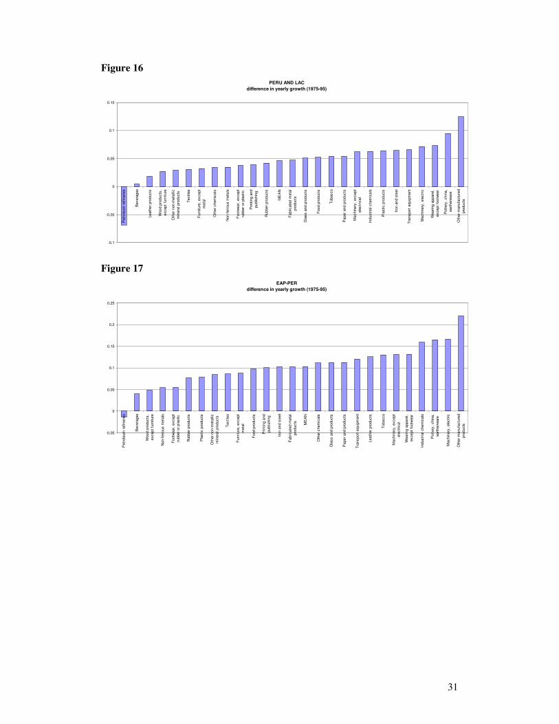
31

Figure 16

PERU AND LAC

difference in yearly growth (1975-95)

-0.1

-0.05

0

0.05

0.1

0.15

Petr

ole

um

refineries

Bevera

ges

Leath

er

pro

ducts

Wood p

roducts

,

except

furn

iture

Oth

er

non-m

eta

llic

min

era

l pro

ducts

Textile

s

Furn

iture

, except

meta

l

Oth

er

chem

icals

Non-f

err

ous m

eta

ls

Footw

ear,

except

rubber

or

pla

stic

Printing a

nd

publis

hin

g

Rubber

pro

ducts

ME

AN

Fabricate

d m

eta

l

pro

ducts

Gla

ss a

nd p

roducts

Food p

roducts

Tobacco

Paper

and p

roducts

Machin

ery

, except

ele

ctr

ical

Industr

ial chem

icals

Pla

stic p

roducts

Iron a

nd s

teel

Tra

nsport

equip

ment

Machin

ery

, ele

ctr

ic

Wearing a

ppare

l,

except

footw

ear

Pott

ery

, chin

a,

eart

henw

are

Oth

er

manufa

ctu

red

pro

ducts

Figure 17

EAP-PER

difference in yearly growth (1975-95)

-0.05

0

0.05

0.1

0.15

0.2

0.25

Petr

ole

um

refineries

Bevera

ges

Wood p

roducts

,

except

furn

iture

Non-f

err

ous m

eta

ls

Footw

ear,

except

rubber

or

pla

stic

Rubber

pro

ducts

Pla

stic p

roducts

Oth

er

non-m

eta

llic

min

era

l pro

ducts

Textile

s

Furn

iture

, except

meta

l

Food p

roducts

Printing a

nd

publis

hin

g

Iron a

nd s

teel

Fabricate

d m

eta

l

pro

ducts ME

AN

Oth

er

chem

icals

Gla

ss a

nd p

roducts

Paper

and p

roducts

Tra

nsport

equip

ment

Leath

er

pro

ducts

Tobacco

Machin

ery

, except

ele

ctr

ical

Wearing a

ppare

l,

except

footw

ear

Industr

ial chem

icals

Pott

ery

, chin

a,

eart

henw

are

Machin

ery

, ele

ctr

ic

Oth

er

manufa

ctu

red

pro

ducts

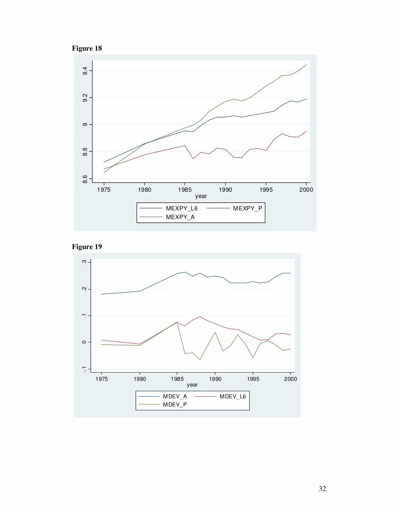
32

Figure 18

Figure 19

-.1

0.1

.2.3

1975 1980 1985 1990 1995 2000year

MDEV_A MDEV_L6

MDEV_P

8.6

8.8

99.2

9.4

1975 1980 1985 1990 1995 2000year

MEXPY_L6 MEXPY_P

MEXPY_A

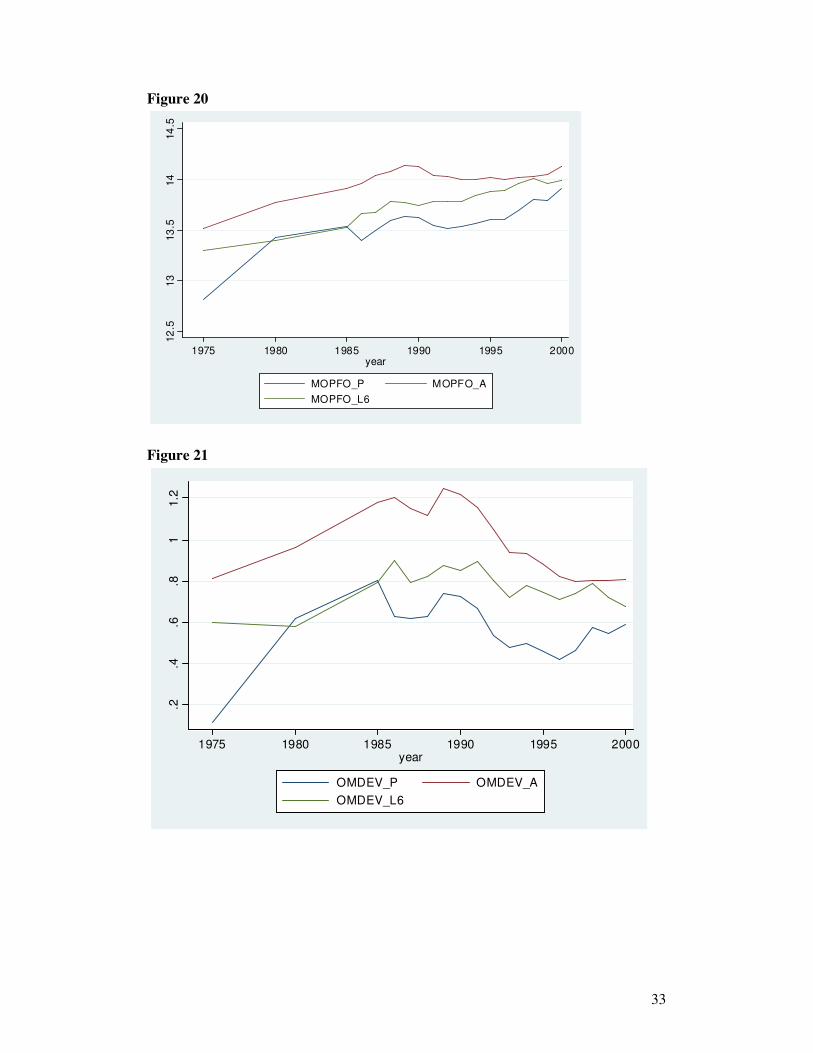
33

Figure 20

Figure 21

.2.4

.6.8

11.2

1975 1980 1985 1990 1995 2000year

OMDEV_P OMDEV_A

OMDEV_L6

12

.513

13

.514

14

.5

1975 1980 1985 1990 1995 2000year

MOPFO_P MOPFO_A

MOPFO_L6

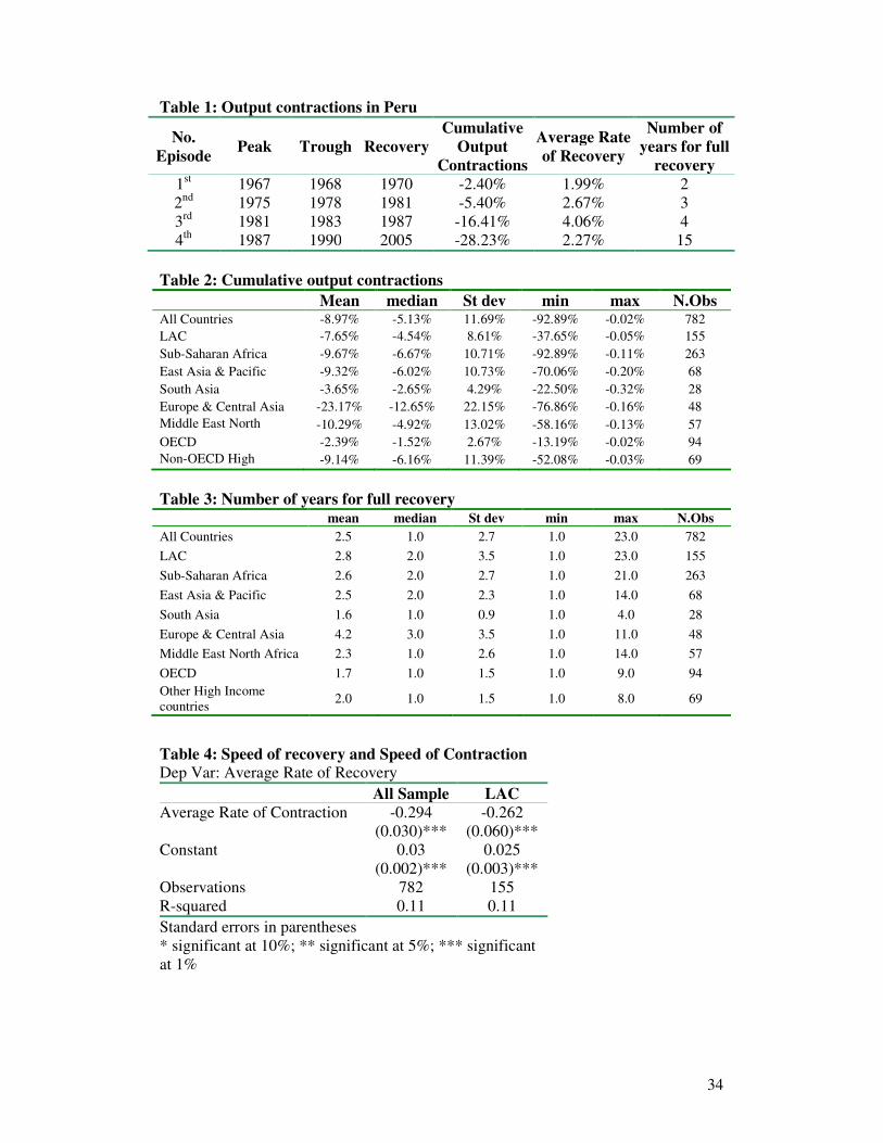
34

Table 1: Output contractions in Peru

No.

Episode Peak Trough Recovery

Cumulative

Output

Contractions

Average Rate

of Recovery

Number of

years for full

recovery

1st 1967 1968 1970 -2.40% 1.99% 2

2nd

1975 1978 1981 -5.40% 2.67% 3

3rd

1981 1983 1987 -16.41% 4.06% 4

4th

1987 1990 2005 -28.23% 2.27% 15

Table 2: Cumulative output contractions

Mean median St dev min max N.Obs All Countries -8.97% -5.13% 11.69% -92.89% -0.02% 782

LAC -7.65% -4.54% 8.61% -37.65% -0.05% 155

Sub-Saharan Africa -9.67% -6.67% 10.71% -92.89% -0.11% 263

East Asia & Pacific -9.32% -6.02% 10.73% -70.06% -0.20% 68

South Asia -3.65% -2.65% 4.29% -22.50% -0.32% 28

Europe & Central Asia -23.17% -12.65% 22.15% -76.86% -0.16% 48

Middle East North

Africa -10.29% -4.92% 13.02% -58.16% -0.13% 57

OECD -2.39% -1.52% 2.67% -13.19% -0.02% 94

Non-OECD High

Income -9.14% -6.16% 11.39% -52.08% -0.03% 69

Table 3: Number of years for full recovery mean median St dev min max N.Obs

All Countries 2.5 1.0 2.7 1.0 23.0 782

LAC 2.8 2.0 3.5 1.0 23.0 155

Sub-Saharan Africa 2.6 2.0 2.7 1.0 21.0 263

East Asia & Pacific 2.5 2.0 2.3 1.0 14.0 68

South Asia 1.6 1.0 0.9 1.0 4.0 28

Europe & Central Asia 4.2 3.0 3.5 1.0 11.0 48

Middle East North Africa 2.3 1.0 2.6 1.0 14.0 57

OECD 1.7 1.0 1.5 1.0 9.0 94

Other High Income

countries 2.0 1.0 1.5 1.0 8.0 69

Table 4: Speed of recovery and Speed of Contraction

Dep Var: Average Rate of Recovery

All Sample LAC

Average Rate of Contraction -0.294 -0.262

(0.030)*** (0.060)***

Constant 0.03 0.025

(0.002)*** (0.003)***

Observations 782 155

R-squared 0.11 0.11

Standard errors in parentheses

* significant at 10%; ** significant at 5%; *** significant

at 1%

35

Table 5: Output contractions in Peru

No.

Episode Peak Trough

Recover

y

Cumulative

Output

Contraction

s

Average

Rate of

Recovery

Number of

years for

full

recovery

Cost of the

Crisis

1st 1967 1968 1970 -2.40% 1.99% 2 0.02

2nd

1975 1978 1981 -5.40% 2.67% 3 0.11

3rd

1981 1983 1987 -16.41% 4.06% 4 0.56

4th

1987 1990 2005 -28.23% 2.27% 15 2.74

Table 6: Cumulative Output Contraction vs. Terms of Trade

(1) (2) (3) (4) (5) (6) (7) (8)

∆TOT 0.089 0.254 0.044 0.233 0.089 0.254 0.083 0.253

(0.039)** (0.059)*** (0.03) (0.063)*** (0.031)*** (0.047)*** (0.030)*** (0.047)***

Constant -0.077 -0.056 -0.078 -0.059 -0.077 -0.056 -0.079 -0.057

(0.006)*** (0.007)*** (0.005)*** (0.010)*** (0.006)*** (0.009)*** (0.006)*** (0.009)***

N. Obs 262 141 262 141 262 141 262 141

Fixed

Effects

No No Country Country No No No No

Sample All ∆TT <0 All ∆TT <0 All ∆TT <0 All ∆TT <0

Method OLS OLS Panel Panel Tobit Tobit Panel

Probit

Panel

Probit

Robust standard errors in parentheses. * significant at 10%; ** significant at 5%; *** significant at 1%

Table 7: Growth and Finance (1) (2) (3) (4) (5) (6) (7) (8)

EXFIN 0.015 0.022 0.014 0.013 0.015 0.022 0.014 0.013 (3.91)*** (2.13)** (3.65)*** (2.45)** (3.91)*** (2.13)** (3.65)*** (2.45)**

EXFIN*LAC -0.011 -0.028 -0.005 -0.014

(2.27)** (1.90)* (0.85) (1.63)

EXFIN*PER 0.010 0.075 0.018 -0.020 -0.000 0.047 0.013 -0.034

(3.63)*** (7.20)*** (4.03)*** (3.20)*** (0.11) (4.47)*** (3.28)*** (6.27)***

EXFIN*OT -0.009 -0.029 -0.003 -0.012

(1.46) (1.79)* (0.32) (0.92)

EXFIN*LA6 -0.012 -0.027 -0.007 -0.015

(2.64)** (1.30) (1.41) (1.85)* Observations 9987 2524 4355 3108 9987 2524 4355 3108

N. of cy 396 104 169 123 396 104 169 123

Period 1974-1996 1974-1979 1980-1989 1990-1996 1974-1996 1974-1979 1980-1989 1990-1996

Robust t statistics in parentheses. Standard errors are clustered at the country-year level. All regressions include country-year

fixed effects. * significant at 10%; ** significant at 5%; *** significant at 1%

Table 8: Growth and Labor Intensity (1) (2) (3) (4) (5) (6) (7) (8)

LI 0.007 -0.021 0.015 0.018 0.007 -0.021 0.015 0.018

(1.10) (2.23)** (1.89)* (1.99)* (1.10) (2.23)** (1.89)* (1.99)*

LI*LAC -0.002 0.026 -0.004 -0.021

(0.22) (2.38)** (0.40) (1.84)* LI*PER -0.011 0.037 -0.038 -0.012 -0.013 0.063 -0.041 -0.033

(4.09)*** (7.10)*** (9.10)*** (1.56) (2.04)* (6.63)*** (5.10)*** (3.75)***

LI*OT -0.005 0.021 -0.004 -0.031 (0.73) (1.87)* (0.41) (2.17)**

LI*LA6 0.006 0.040 -0.004 -0.008

(0.64) (3.38)*** (0.29) (0.61) Observations 13068 3441 5886 3741 13068 3441 5886 3741

N. of cy 533 142 237 154 533 142 237 154

Period 1974-1996 1974-1979 1980-1989 1990-1996 1974-1996 1974-1979 1980-1989 1990-1996



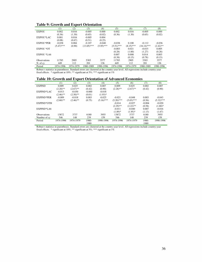
36

Table 9: Growth and Export Orientation (1) (2) (3) (4) (5) (6) (7) (8)

EXPOU 0.002 0.016 -0.005 0.000 0.002 0.016 -0.005 0.000

(0.36) (1.30) (0.65) (0.02) (0.36) (1.30) (0.65) (0.02)

EXPOU*LAC 0.001 0.016 -0.005 0.004 (0.08) (0.67) (0.51) (0.25)

EXPOU*PER -0.038 0.084 -0.107 -0.040 -0.038 0.100 -0.112 -0.036

(5.47)*** (0.90) (13.05)*** (5.95)*** (5.51)*** (8.15)*** (16.14)*** (2.42)** EXPOU *OT -0.003 0.021 -0.015 0.005

(0.28) (1.00) (1.27) (0.28)

EXPOU *LA6 0.007 0.008 0.014 0.003 (0.38) (0.15) (0.78) (0.15)

Observations 11785 2905 5303 3577 11785 2905 5303 3577

N. of cy 449 112 201 136 449 112 201 136

Period 1974-1996 1974-1979 1980-1989 1990-1996 1974-1996 1974-1979 1980-1989 1990-1996

Robust t statistics in parentheses. Standard errors are clustered at the country-year level. All regressions include country-year fixed effects. * significant at 10%; ** significant at 5%; *** significant at 1%

Table 10: Growth and Export Orientation of Advanced Economies

(1) (2) (3) (4) (5) (6) (7) (8)

EXPIND 0.009 0.025 0.002 0.007 0.009 0.025 0.002 0.007

(2.28)** (2.67)** (0.42) (0.90) (2.28)** (2.67)** (0.42) (0.90) EXPIND*LAC -0.013 -0.030 -0.000 -0.018

(2.46)** (2.50)** (0.01) (1.93)*

EXPIND*PER -0.009 -0.018 0.003 -0.025 -0.021 -0.048 0.003 -0.043 (2.68)** (2.46)** (0.75) (5.16)*** (5.20)*** (5.03)*** (0.56) (5.32)***

EXPIND*OTH -0.014 -0.027 -0.004 -0.020

(2.29)** (2.22)** (0.58) (1.80)*

EXPIND*LA6 -0.011 -0.040 0.007 -0.016

(1.89)* (1.95)* (1.13) (1.67)

Observations 13872 3737 6180 3955 13872 3737 6180 3955

Number of cy 546 148 239 159 546 148 239 159

Period 1974-1996 1974-1979 1980-

1989

1990-1996 1974-1996 1974-1979 1980-

1989

1990-1996



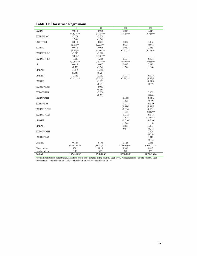
37

Table 11: Horserace Regressions (1) (2) (3) (4)

EXFIN 0.014 0.014 0.014 0.014

(4.82)*** (5.72)*** (4.82)*** (5.72)***

EXFIN*LAC -0.009 -0.008 (1.74)* (1.56)

EXIN*PER 0.011 0.010 0.002 0.002

(2.63)** (2.29)** (0.73) (0.91) EXPIND 0.012 0.015 0.012 0.015

(2.72)** (4.10)*** (2.72)** (4.10)***

EXPINF*LAC -0.013 -0.018 (2.04)* (3.38)***

EXPIND*PER -0.017 -0.015 -0.031 -0.033

(3.70)*** (3.83)*** (6.89)*** (9.08)***

LI 0.013 0.010 0.013 0.010

(1.70) (1.36) (1.70) (1.36)

LI*LAC -0.005 -0.002

(0.65) (0.25)

LI*PER -0.013 -0.012 -0.018 -0.015

(3.65)*** (2.66)** (2.38)** (1.92)* EXPOU -0.005 -0.005

(0.77) (0.77)

EXPOU*LAC 0.009 (0.69)

EXPOU*PER -0.009 0.000

(0.79) (0.04) EXFIN*OTH -0.008 -0.006

(1.02) (0.79)

EXFIN*LA6 -0.011 -0.010

(1.98)* (1.98)*

EXPIND*OTH -0.014 -0.021

(1.72) (3.84)***

EXPIND*LA6 -0.012 -0.015

(1.65) (2.16)**

LI*OTH -0.010 -0.010 (1.26) (1.13)

LI*LA6 0.000 0.003

(0.04) (0.31) EXPOU*OTH 0.006

(0.28) EXPOU*LA6 0.010

(0.75)

Constant 0.129 0.136 0.128 0.135 (339.23)*** (48.05)*** (153.96)*** (40.87)***

Observations 9502 8815 9502 8815

Number of cy 396 355 396 355

Period 1974-1996 1974-1996 1974-1996 1974-1996



Documents

PERUVIAN ECONOMIC ASSOCIATION Peru’s Great …perueconomics.org/wp-content/uploads/2014/01/WP-45.pdf1 Peru's Great Depression A Perfect Storm? Gonzalo Llosa and Ugo Panizza * The