Embed Size (px)
Citation preview
PhD Course: Structural VAR models
II. Specification, estimation procedure and information content
Hilde C. Bjørnland
Norwegian School of Management (BI)

Lecture note II: Specification, estimation procedure and information content
Content
1. Response to forecast errors 2. Impulse response functions
From Structural VAR to structural moving average (SMA) representation Orthogonal decomposition Implementation
3. Forecast error variance decomposition 4. Empirical examples
Choleski recursive decomposition Does the ordering of the variables matter? Additional variables? etc.
VAR models concentrate on shocks. First, the relevant shocks are identified and the response of the system to shocks is described by analyzing impulse responses (the propagation mechanism of shocks), forecast error variance decomposition, and historical decomposition. The structural form of the model can then be conveniently summarized by the impulse response functions and the variance decomposition. The impulse response function describes the in-sample effect of a typical shock to the system and can be used to economically interpret the behavior of the system. The variance decomposition assesses the importance of different shocks by determining the relative share of variance that each structural shock contributes to the total variance of each variable.
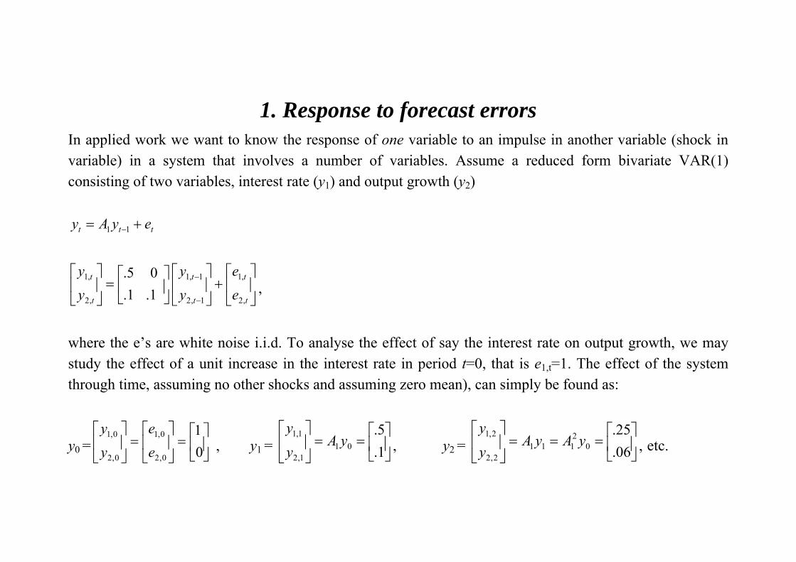
1. Response to forecast errors In applied work we want to know the response of one variable to an impulse in another variable (shock in variable) in a system that involves a number of variables. Assume a reduced form bivariate VAR(1) consisting of two variables, interest rate (y1) and output growth (y2)
ttt eyAy += −11
⎥⎦
⎤⎢⎣
⎡+⎥
⎦
⎤⎢⎣
⎡⎥⎦
⎤⎢⎣
⎡=⎥
⎦
⎤⎢⎣
⎡
−
−
t
t
t
t
t
t
ee
yy
yy
,2
,1
1,2
1,1
,2
,1
1.1.05.
,
where the e’s are white noise i.i.d. To analyse the effect of say the interest rate on output growth, we may study the effect of a unit increase in the interest rate in period t=0, that is e1,t=1. The effect of the system through time, assuming no other shocks and assuming zero mean), can simply be found as:
y0 = , y1 = , y2 = , etc. ⎥⎦
⎤⎢⎣
⎡=⎥
⎦
⎤⎢⎣
⎡=⎥
⎦
⎤⎢⎣
⎡
01
0,2
0,1
0,2
0,1
ee
yy
⎥⎦
⎤⎢⎣
⎡==⎥
⎦
⎤⎢⎣
⎡
1.5.
011,2
1,1 yAyy
⎥⎦
⎤⎢⎣
⎡===⎥
⎦
⎤⎢⎣
⎡
06.25.
02
1112,2
2,1 yAyAyy
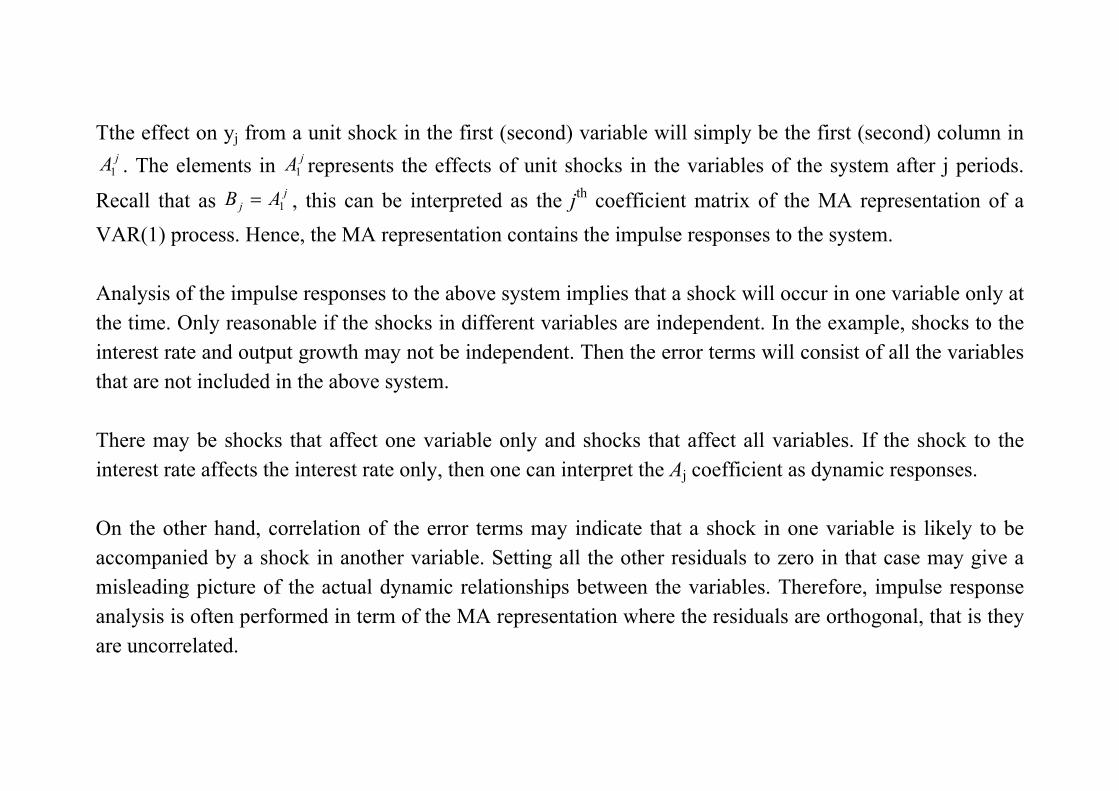
Tthe effect on yj from a unit shock in the first (second) variable will simply be the first (second) column in . The elements in represents the effects of unit shocks in the variables of the system after j periods.
Recall that as , this can be interpreted as the jth coefficient matrix of the MA representation of a VAR(1) process. Hence, the MA representation contains the impulse responses to the system.
jA1jA1
jj AB 1=
Analysis of the impulse responses to the above system implies that a shock will occur in one variable only at the time. Only reasonable if the shocks in different variables are independent. In the example, shocks to the interest rate and output growth may not be independent. Then the error terms will consist of all the variables that are not included in the above system. There may be shocks that affect one variable only and shocks that affect all variables. If the shock to the interest rate affects the interest rate only, then one can interpret the Aj coefficient as dynamic responses. On the other hand, correlation of the error terms may indicate that a shock in one variable is likely to be accompanied by a shock in another variable. Setting all the other residuals to zero in that case may give a misleading picture of the actual dynamic relationships between the variables. Therefore, impulse response analysis is often performed in term of the MA representation where the residuals are orthogonal, that is they are uncorrelated.
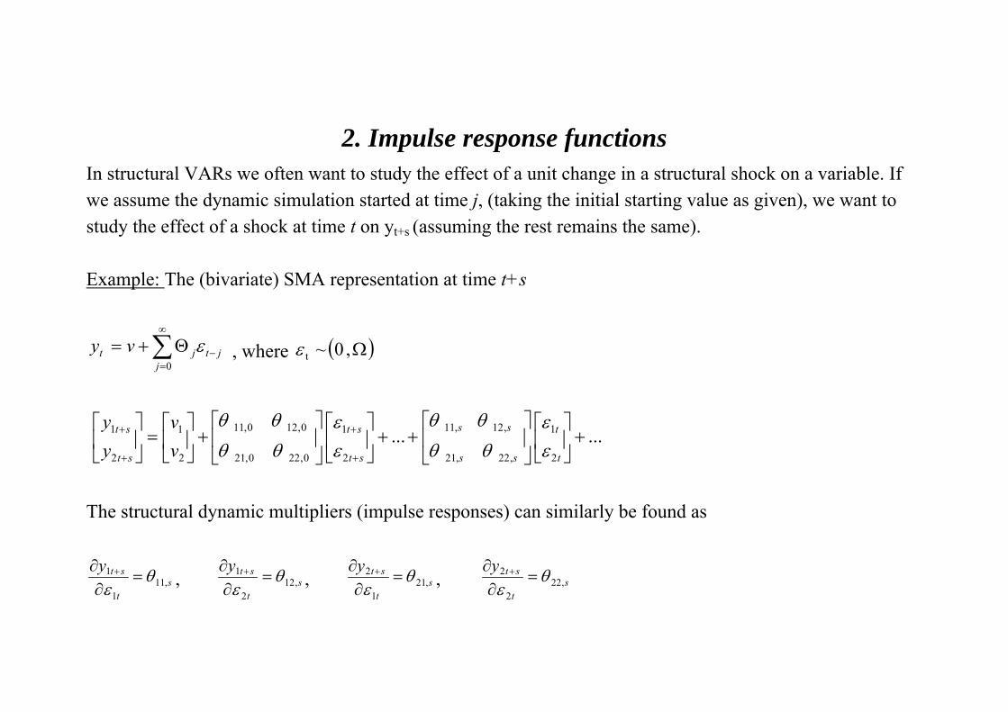
2. Impulse response functions In structural VARs we often want to study the effect of a unit change in a structural shock on a variable. If we assume the dynamic simulation started at time j, (taking the initial starting value as given), we want to study the effect of a shock at time t on yt+s (assuming the rest remains the same). Example: The (bivariate) SMA representation at time t+s
∑∞
=−Θ+=
0jjtjt vy ε , where ( )Ω,0~tε
......2
1
,22,21
,12,11
2
1
0,220,21
0,120,11
2
1
2
1 +⎥⎦
⎤⎢⎣
⎡⎥⎦
⎤⎢⎣
⎡++⎥
⎦
⎤⎢⎣
⎡⎥⎦
⎤⎢⎣
⎡+⎥
⎦
⎤⎢⎣
⎡=⎥
⎦
⎤⎢⎣
⎡
+
+
+
+
t
t
ss
ss
st
st
st
st
vv
yy
εε
θθθθ
εε
θθθθ
The structural dynamic multipliers (impulse responses) can similarly be found as
st
sty,11
1
1 θε
=∂∂ + , s
t
sty,12
2
1 θε
=∂∂ + , s
t
sty,21
1
2 θε
=∂∂ + , s
t
sty,22
2
2 θε
=∂∂ +

The dynamic multiplier depends only on s, the length of time separating the disturbance to the input (εt) and the observed value of output (yt+s). The impulse response functions (IRFs) of the structural shocks will be the plots of θij,s for i,j = 1, 2. These plots summarize how unit impulses of the structural shocks at time t impact the level of y at time t+s for different values of s. Recall that a univariate AR(1) process can be viewed as an MA(∞) process. Stationarity of yt implies
0lim , =∞→ sijsθ .
The long run cumulative impact of the structural shocks can be found as:
⎥⎦
⎤⎢⎣
⎡=
⎥⎥⎥⎥
⎦
⎤
⎢⎢⎢⎢
⎣
⎡
=
⎥⎥⎥⎥
⎦
⎤
⎢⎢⎢⎢
⎣
⎡
∂∂
∂∂
∂∂
∂∂
=Θ
∑∑
∑∑
∑∑
∑∑∞
=
∞
=
∞
=
∞
=
∞
=
+∞
=
+
∞
=
+∞
=
+
)1()1()1()1(
)1(2221
1211
0,22
0,21
0,12
0,11
0 2
2
0 1
2
0 2
1
0 1
1
θθθθ
θθ
θθ
εε
εε
ss
ss
ss
ss
s t
st
s t
st
s t
st
s t
st
yy
yy
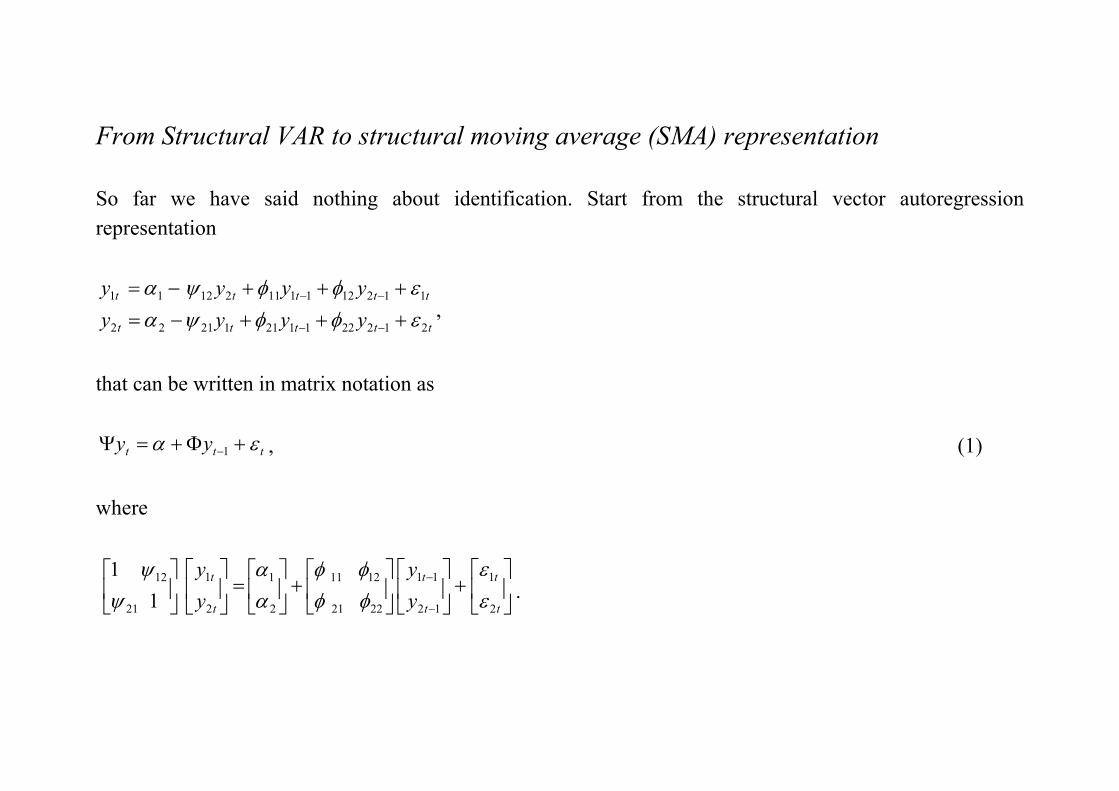
From Structural VAR to structural moving average (SMA) representation So far we have said nothing about identification. Start from the structural vector autoregression representation
ttttt
ttttt
yyyyyyyy
21222112112122
11212111121211
εφφψαεφφψα
+++−=+++−=
−−
−−,
that can be written in matrix notation as
ttt yy εα +Φ+=Ψ −1 , (1) where
⎥⎦
⎤⎢⎣
⎡+⎥
⎦
⎤⎢⎣
⎡⎥⎦
⎤⎢⎣
⎡+⎥
⎦
⎤⎢⎣
⎡=⎥
⎦
⎤⎢⎣
⎡⎥⎦
⎤⎢⎣
⎡
−
−
t
t
t
t
t
t
yy
yy
2
1
12
11
2221
1211
2
1
2
1
21
12
11
εε
φφφφ
αα
ψψ
.
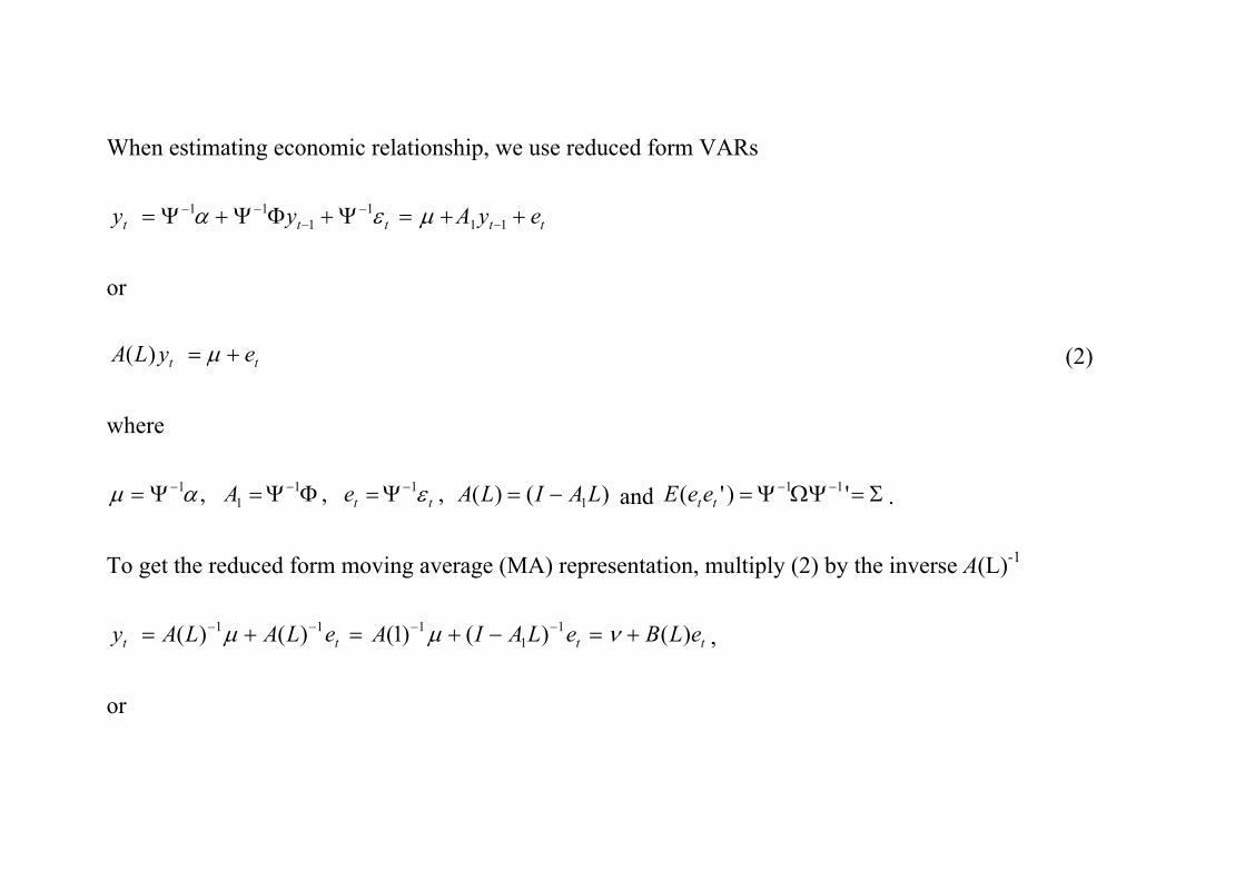
When estimating economic relationship, we use reduced form VARs
ttttt eyAyy ++=Ψ+ΦΨ+Ψ= −−
−−−
111
111 μεα
or
tt eyLA += μ)( (2) where
)()(,,, 111
11 LAILAeA tt −=Ψ=ΦΨ=Ψ= −−− εαμ and . Σ=ΩΨΨ= −− ')'( 11
tteeE
To get the reduced form moving average (MA) representation, multiply (2) by the inverse A(L)-1
tttt eLBeLAIAeLALAy )()()1()()( 11
111 +=−+=+= −−−− νμμ , or
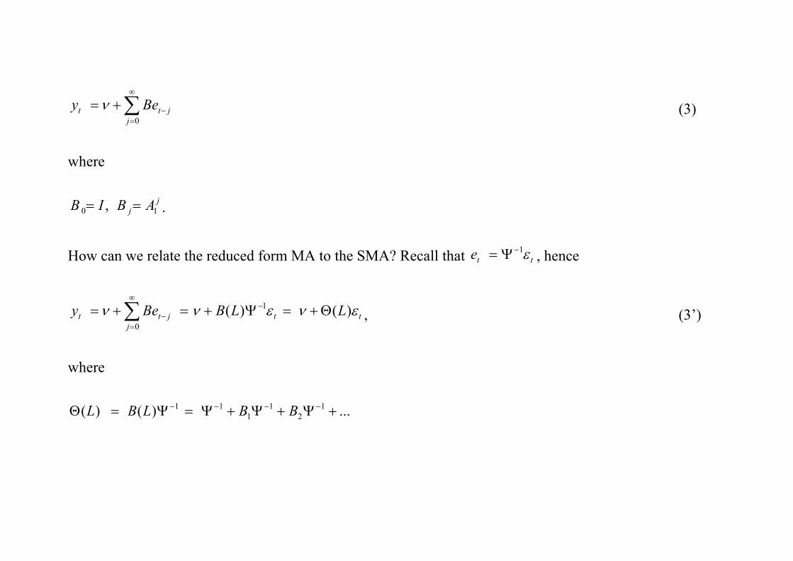
∑∞
=−+=
0jjtt Bey ν (3)
where
jj ABIB 10 , == .
How can we relate the reduced form MA to the SMA? Recall that , hence tte ε1−Ψ=
ttj
jtt LLBBey ενενν )()( 1
0
Θ+=Ψ+=+= −∞
=−∑ , (3’)
where
...)()( 12
11
11 +Ψ+Ψ+Ψ=Ψ=Θ −−−− BBLBL
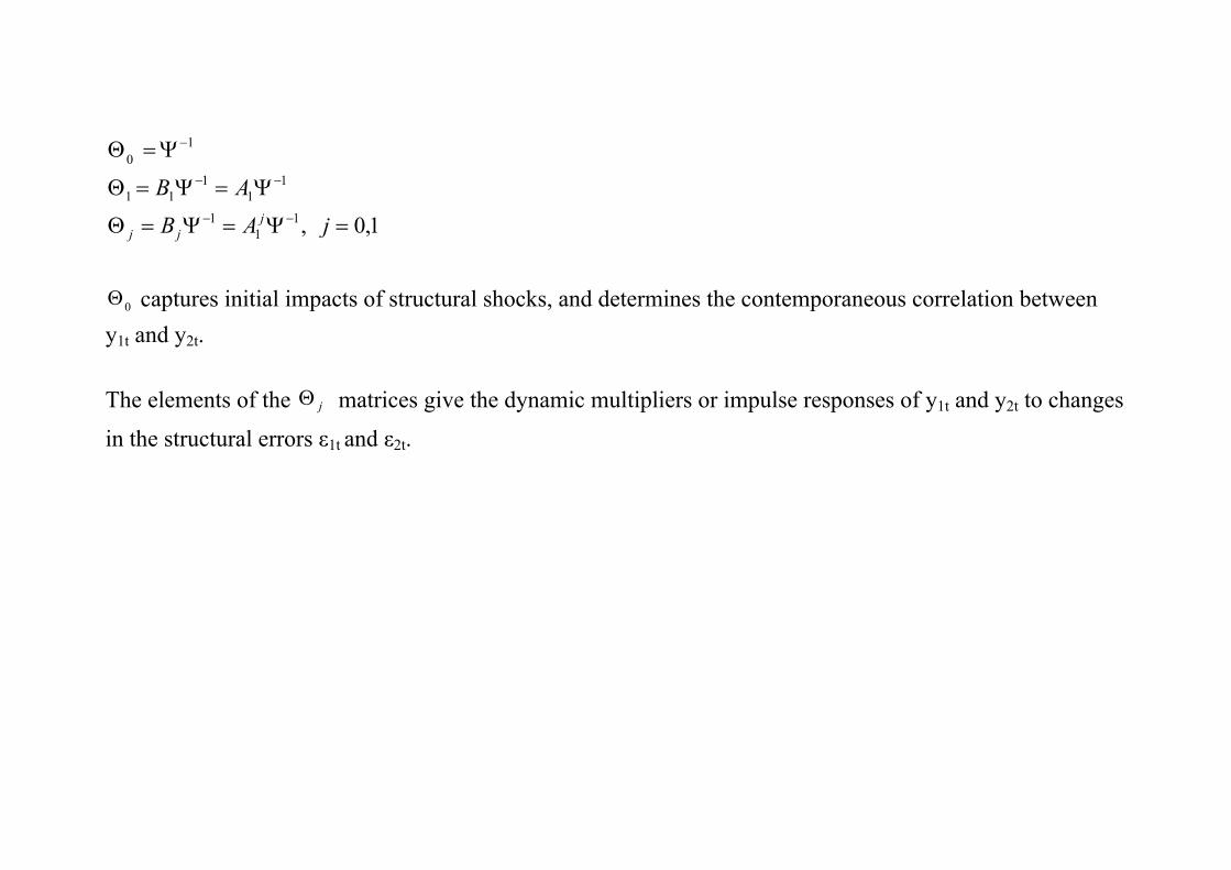
1,0,11
1
11
111
10
=Ψ=Ψ=Θ
Ψ=Ψ=Θ
Ψ=Θ
−−
−−
−
jAB
ABj
jj
0Θ captures initial impacts of structural shocks, and determines the contemporaneous correlation between
y1t and y2t. The elements of the matrices give the dynamic multipliers or impulse responses of y1t and y2t to changes
in the structural errors ε1t and ε2t.jΘ

Orthogonal decomposition Assume (again) the reduced form MA representation:
∑∞
=−+=
0iitit eBy ν (3)
where et is a white noise process with non-singular covariance matrix Σ . Assume the positive definite symmetric matrix can be written as the product 'PP=Σ , where P is a lower triangular non-singular matrix with positive diagonal elements. This decomposition is called the Choleski decomposition. Using this, (3) can be rewritten as:
∑
∑∞
=−
∞
=−
−
+=
+=
0
0
1
iiti
iitit
vC
ePPBy
ν
ν
(4)
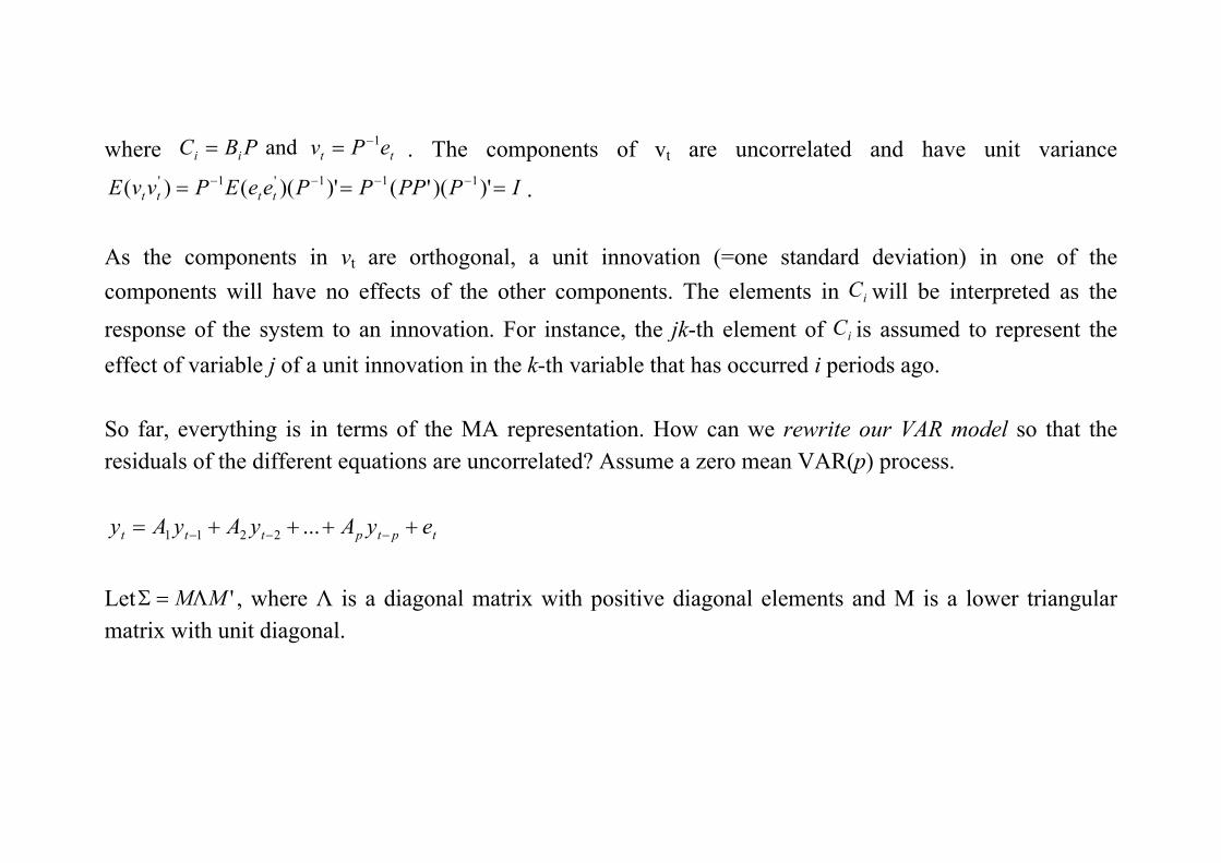
where . The components of vt are uncorrelated and have unit variance
. ttii ePvPBC 1and −==
IPPPPPeeEPvvE tttt === −−−− )')('()')(()( 111'1'
As the components in vt are orthogonal, a unit innovation (=one standard deviation) in one of the components will have no effects of the other components. The elements in will be interpreted as the response of the system to an innovation. For instance, the jk-th element of is assumed to represent the effect of variable j of a unit innovation in the k-th variable that has occurred i periods ago.
iC
iC
So far, everything is in terms of the MA representation. How can we rewrite our VAR model so that the residuals of the different equations are uncorrelated? Assume a zero mean VAR(p) process.
tptpttt eyAyAyAy ++++= −−− ...2211 Let 'MMΛ=Σ , where Λ is a diagonal matrix with positive diagonal elements and Μ is a lower triangular matrix with unit diagonal.
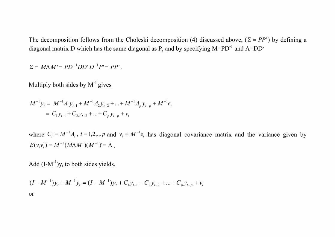
The decomposition follows from the Choleski decomposition (4) discussed above, ( 'PP=Σ ) by defining a diagonal matrix D which has the same diagonal as P, and by specifying M=PD-1 and Λ=DD׳
'''' 11 PPPDDDPDMM ==Λ=Σ −− . Multiply both sides by M-1 gives
tptptt
tptpttt
vyCyCyC
eMyAMyAMyAMyM
++++=
++++=
−−−
−−
−−
−−
−−
...
...
2211
1122
111
11
where and has diagonal covariance matrix and the variance given by
.
piAMC ii ,...2,1,1 == −tt eMv 1−=
Λ=Λ= −− )')('()( 11' MMMMvvE tt
Add (I-M-1)yt to both sides yields,
tptpttttt vyCyCyCyMIyMyMI +++++−=+− −−−−−− ...)()( 2211
111 or
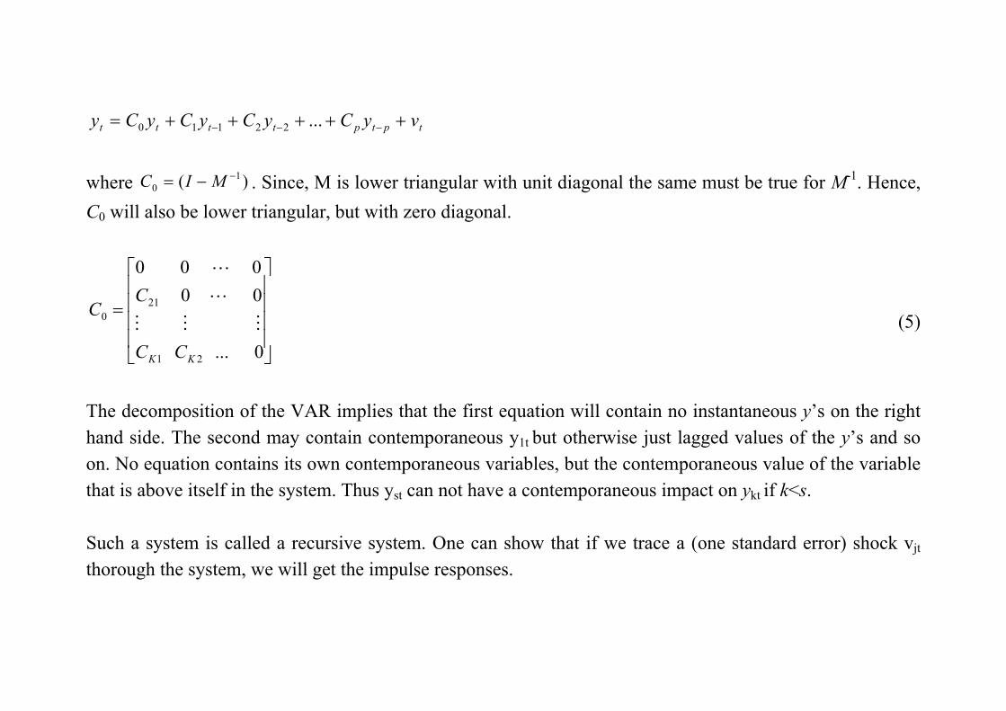
tptptttt vyCyCyCyCy +++++= −−− ...22110 where . Since, M is lower triangular with unit diagonal the same must be true for M-1. Hence, C0 will also be lower triangular, but with zero diagonal.
)( 10
−−= MIC
⎥⎥⎥⎥
⎦
⎤
⎢⎢⎢⎢
⎣
⎡
=
0...
00000
21
210
KK CC
CC
MMM
L
L
(5)
The decomposition of the VAR implies that the first equation will contain no instantaneous y’s on the right hand side. The second may contain contemporaneous y1t but otherwise just lagged values of the y’s and so on. No equation contains its own contemporaneous variables, but the contemporaneous value of the variable that is above itself in the system. Thus yst can not have a contemporaneous impact on ykt if k<s. Such a system is called a recursive system. One can show that if we trace a (one standard error) shock vjt thorough the system, we will get the impulse responses.
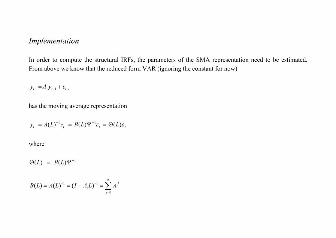
Implementation In order to compute the structural IRFs, the parameters of the SMA representation need to be estimated. From above we know that the reduced form VAR (ignoring the constant for now)
ttt eyAy += −11 , has the moving average representation
tttt LLBeLAy εε )()()( 11 Θ=Ψ== −− where
∑∞
=
−−
−
=−==
Ψ=Θ
01
11
1
1
)()()(
)()(
j
jALAILALB
LBL
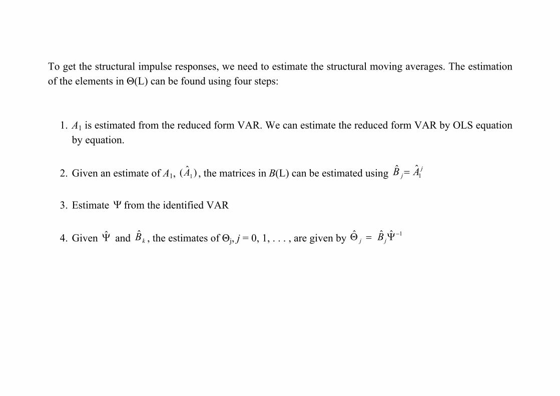
To get the structural impulse responses, we need to estimate the structural moving averages. The estimation of the elements in Θ(L) can be found using four steps:
1. A1 is estimated from the reduced form VAR. We can estimate the reduced form VAR by OLS equation by equation.
2. Given an estimate of A1, , the matrices in B(L) can be estimated using )ˆ( 1A jj AB 1
ˆˆ =
3. Estimate Ψ from the identified VAR
4. Given Ψ̂ and , the estimates of Θj, j = 0, 1, . . . , are given by kB̂ 1ˆˆˆ −Ψ=Θ jj B
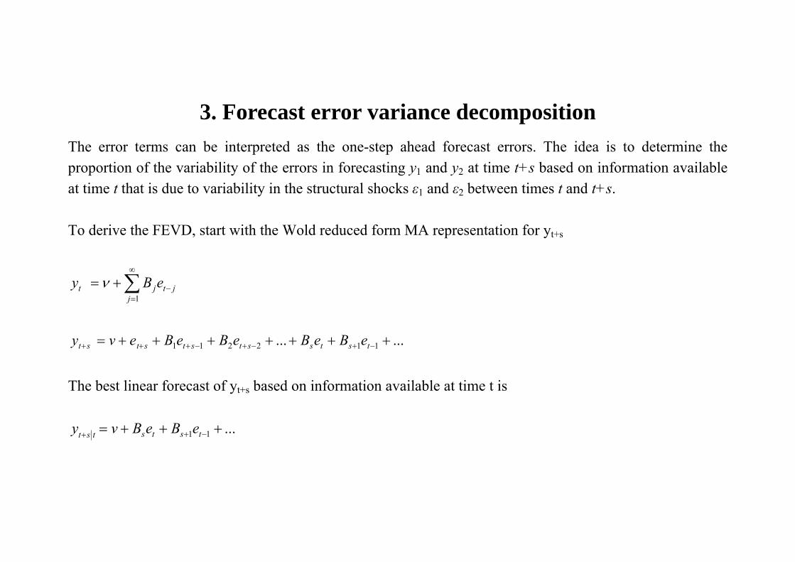
3. Forecast error variance decomposition The error terms can be interpreted as the one-step ahead forecast errors. The idea is to determine the proportion of the variability of the errors in forecasting y1 and y2 at time t+s based on information available at time t that is due to variability in the structural shocks ε1 and ε2 between times t and t+s. To derive the FEVD, start with the Wold reduced form MA representation for yt+s
jtj
jt eBy −
∞
=∑+=
1
ν
...... 112211 +++++++= −+−+−+++ tstsstststst eBeBeBeBevy
The best linear forecast of yt+s based on information available at time t is
...11 +++= −++ tststst eBeBvy
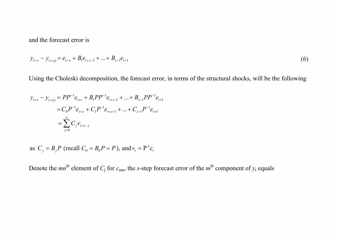
and the forecast error is
1111 ... +−−++++ +++=− tsststtstst eBeBeyy (6)
Using the Choleski decomposition, the forecast error, in terms of the structural shocks, will be the following
Pand),recall( as
...
...
1-00
0
11
111
11
0
11
111
11
ttjj
jjstj
tsstst
tsststtstst
vPPBCPBC
vC
PCPCPC
ePPBePPBePPyy
ε
εεε
====
=
+++=
+++=−
∑∞
=−+
+−
−−+−
+−
+−
−−+−
+−
++
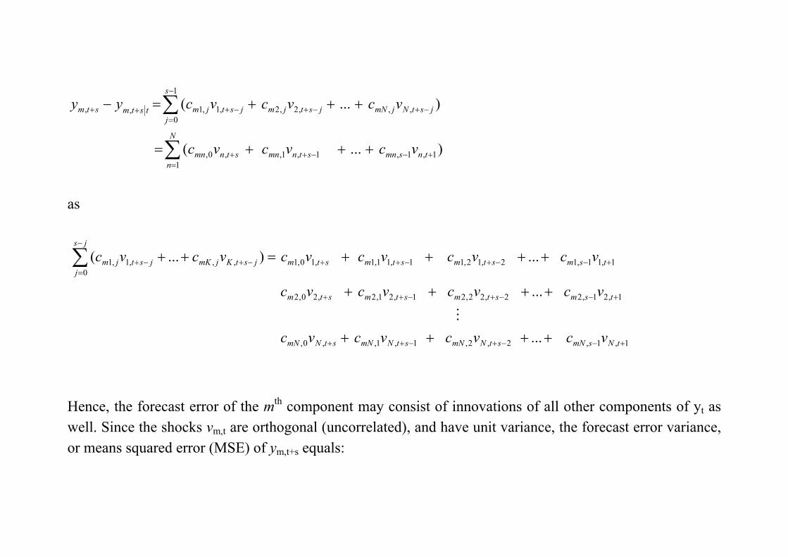
Denote the mnth element of Cj for cmn, the s-step forecast error of the mth component of yt equals
)...(
)...(
1,1,1,1,1
,0,
,,,2,2
1
0,1,1,,
+−−+=
+
−+−+
−
=−+++
+++=
+++=−
∑
∑
tnsmnstnmn
N
nstnmn
jstNjmNjstjm
s
jjstjmtstmstm
vcvcvc
vcvcvcyy
as
1,1,2,2,1,1,,0,
1,21,22,22,21,21,2,20,2
1,11,12,12,11,11,1,10,1,,0
,1,1
...
...
...)...(
+−−+−++
+−−+−++
+−−+−++−+
−
=−+
++++
++++
++++=++∑
tNsmNstNmNstNmNstNmN
tsmstmstmstm
tsmstmstmstmjstKjmK
js
jjstjm
vcvcvcvc
vcvcvcvc
vcvcvcvcvcvc
M
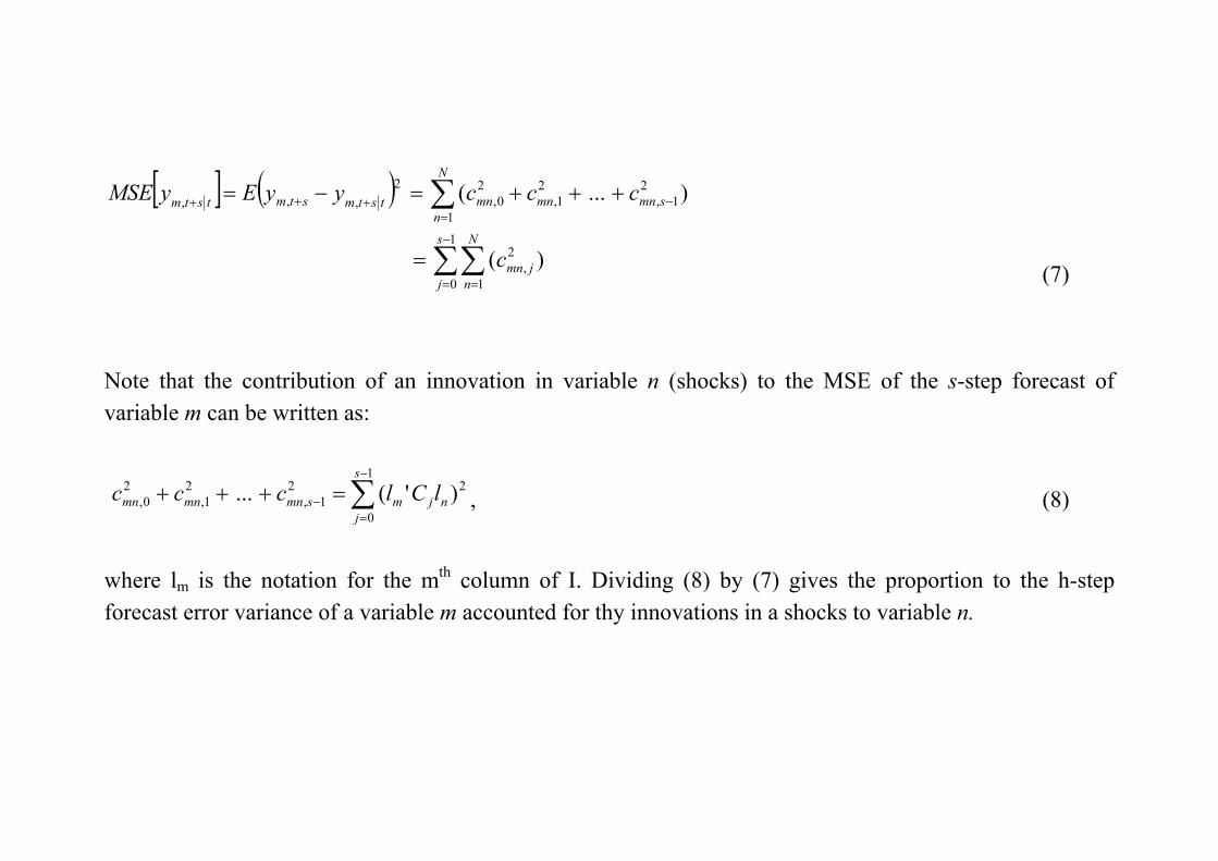
Hence, the forecast error of the mth component may consist of innovations of all other components of yt as well. Since the shocks vm,t are orthogonal (uncorrelated), and have unit variance, the forecast error variance, or means squared error (MSE) of ym,t+s equals:
[ ] ( )
)(
)...(
1
0 1
2,
21,
21,
1
20,
2,,,
∑∑
∑−
= =
−=
+++
=
+++=−=
s
j
N
njmn
smnmn
N
nmntstmstmtstm
c
cccyyEyMSE
(7)
Note that the contribution of an innovation in variable n (shocks) to the MSE of the s-step forecast of variable m can be written as:
21
0
21,
21,
20, )'(... nj
s
jmsmnmnmn lClccc ∑
−
=− =+++ , (8)
where lm is the notation for the mth column of I. Dividing (8) by (7) gives the proportion to the h-step forecast error variance of a variable m accounted for thy innovations in a shocks to variable n.

[ ]stm
nj
s
jm
smn yMSE
lCl
+
−
=∑
=Γ,
21
0,
)'(
(9)
From (9) we can interpret the forecast error variance as being decomposed into components accounted for by innovations in the different variables of the system. Hence, the s-step forecast MSE matrix is seen to be
[ ] ''1
0
1
0j
s
jjj
s
jjtst BBCCyMSE ∑∑
−
=
−
=+ Σ==
The diagonal elements of this matrix are the MSEs of the ymt variables that can be used in (9).
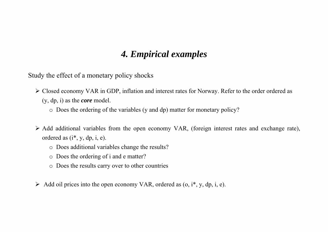
4. Empirical examples Study the effect of a monetary policy shocks
Closed economy VAR in GDP, inflation and interest rates for Norway. Refer to the order ordered as (y, dp, i) as the core model.
o Does the ordering of the variables (y and dp) matter for monetary policy?
Add additional variables from the open economy VAR, (foreign interest rates and exchange rate), ordered as (i*, y, dp, i, e).
o Does additional variables change the results? o Does the ordering of i and e matter? o Does the results carry over to other countries
Add oil prices into the open economy VAR, ordered as (o, i*, y, dp, i, e).
In this exercise, data and additional explanations can be found in:
Bjørnland, H.C. (2005), “Monetary Policy and Exchange Rate Interactions in a Small Open Economy,” Working Paper 2005/16, Norges Bank.
Bjørnland, H.C. (2006), “Monetary policy and exchange rate overshooting: Dornbusch was right after all”, Manuscript, University of Oslo.
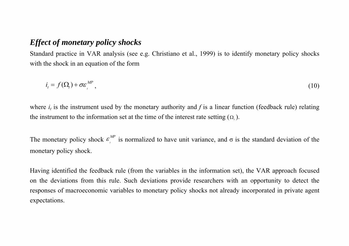
Effect of monetary policy shocks Standard practice in VAR analysis (see e.g. Christiano et al., 1999) is to identify monetary policy shocks with the shock in an equation of the form
( )t
MPt ti f σε= Ω + , (10)
where it is the instrument used by the monetary authority and f is a linear function (feedback rule) relating the instrument to the information set at the time of the interest rate setting ( tΩ ).
The monetary policy shock t
MPε is normalized to have unit variance, and σ is the standard deviation of the
monetary policy shock. Having identified the feedback rule (from the variables in the information set), the VAR approach focused on the deviations from this rule. Such deviations provide researchers with an opportunity to detect the responses of macroeconomic variables to monetary policy shocks not already incorporated in private agent expectations.

Figure 1. Responses to a 1 pp. monetary policy shock; Alternative Choleski orderings a) Interest rate (core) b) GDP and inflation (core)
-0.2
0
0.2
0.4
0.6
0.8
1
1.2
1 2 3 4 5 6 7 8 9 10 11 12 13 14 15 16 17 18 19 20 21 22 23 24
Interest rate (core)
-0.2
-0.15
-0.1
-0.05
0
0.05
1 2 3 4 5 6 7 8 9 10 11 12 13 14 15 16 17 18 19 20 21 22 23 24
GDP (core)Inflation (core)
c) Interest rate (dp-y-i) d) GDP and inflation (dp-y-i)
-0.2
0
0.2
0.4
0.6
0.8
1
1.2
1 2 3 4 5 6 7 8 9 10 11 12 13 14 15 16 17 18 19 20 21 22 23 24
Interest rate (dp,y,i)
-0.2
-0.15
-0.1
-0.05
0
0.05
1 2 3 4 5 6 7 8 9 10 11 12 13 14 15 16 17 18 19 20 21 22 23 24
Inflation (dp,y,i)GDP (dp,y,i)
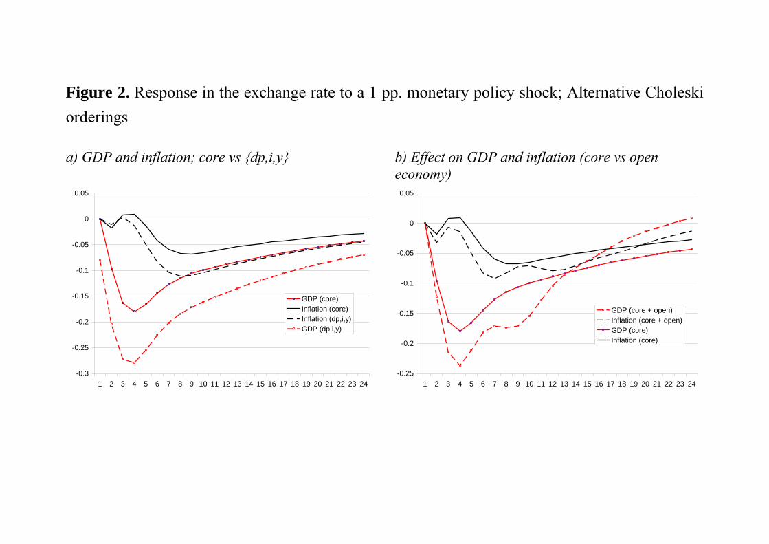
Figure 2. Response in the exchange rate to a 1 pp. monetary policy shock; Alternative Choleski orderings a) GDP and inflation; core vs {dp,i,y} b) Effect on GDP and inflation (core vs open
economy)
-0.3
-0.25
-0.2
-0.15
-0.1
-0.05
0
0.05
1 2 3 4 5 6 7 8 9 10 11 12 13 14 15 16 17 18 19 20 21 22 23 24
GDP (core)Inflation (core)Inflation (dp,i,y)GDP (dp,i,y)
-0.25
-0.2
-0.15
-0.1
-0.05
0
0.05
1 2 3 4 5 6 7 8 9 10 11 12 13 14 15 16 17 18 19 20 21 22 23 24
GDP (core + open)Inflation (core + open)GDP (core)Inflation (core)
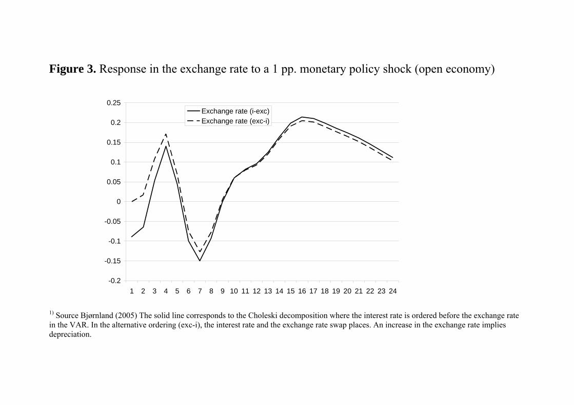
Figure 3. Response in the exchange rate to a 1 pp. monetary policy shock (open economy)
-0.2
-0.15
-0.1
-0.05
0
0.05
0.1
0.15
0.2
0.25
1 2 3 4 5 6 7 8 9 10 11 12 13 14 15 16 17 18 19 20 21 22 23 24
Exchange rate (i-exc)Exchange rate (exc-i)
1) Source Bjørnland (2005) The solid line corresponds to the Choleski decomposition where the interest rate is ordered before the exchange rate in the VAR. In the alternative ordering (exc-i), the interest rate and the exchange rate swap places. An increase in the exchange rate implies depreciation.
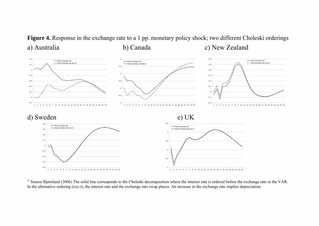
Figure 4. Response in the exchange rate to a 1 pp. monetary policy shock; two different Choleski orderings a) Australia b) Canada c) New Zealand
-0.2
0
0.2
0.4
0.6
0.8
1
1.2
1.4
1 2 3 4 5 6 7 8 9 10 11 12 13 14 15 16 17 18 19 20 21 22 23 24
Real exchange rateReal exchange rate (exc-i)
-1
-0.5
0
0.5
1
1.5
2
1 2 3 4 5 6 7 8 9 10 11 12 13 14 15 16 17 18 19 20 21 22 23 24
Real exchange rateReal exchange rate (exc-i)
-0.2
-0.1
0
0.1
0.2
0.3
0.4
0.5
0.6
1 2 3 4 5 6 7 8 9 10 11 12 13 14 15 16 17 18 19 20 21 22 23 24
Real exchange rateReal exchange rate (exc-i)
d) Sweden e) UK
-0.4
-0.3
-0.2
-0.1
0
0.1
0.2
0.3
0.4
1 2 3 4 5 6 7 8 9 10 11 12 13 14 15 16 17 18 19 20 21 22 23 24
Real exchange rateReal exchange rate (exc-i)
-1
-0.5
0
0.5
1
1.5
1 2 3 4 5 6 7 8 9 10 11 12 13 14 15 16 17 18 19 20 21 22 23 24
Real exchange rate Real exchange rate (exc-i)
1) Source Bjørnland (2006) The solid line corresponds to the Choleski decomposition where the interest rate is ordered before the exchange rate in the VAR. In the alternative ordering (exc-i), the interest rate and the exchange rate swap places. An increase in the exchange rate implies depreciation.
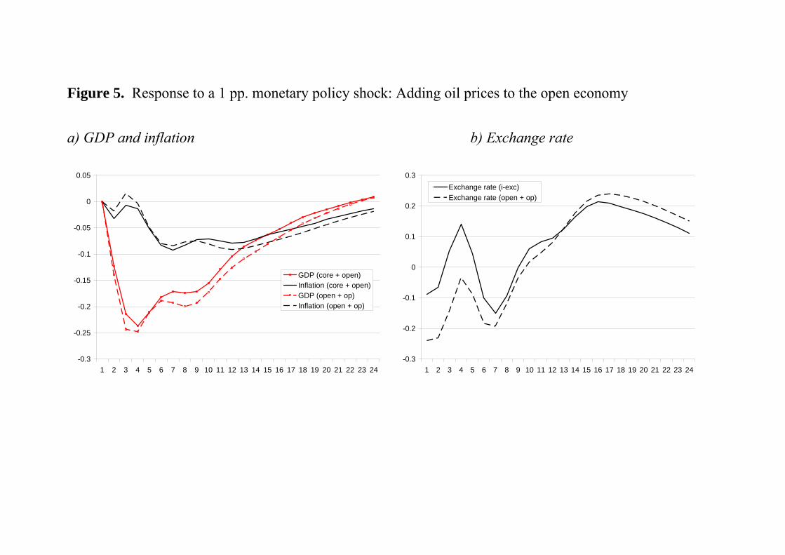
Figure 5. Response to a 1 pp. monetary policy shock: Adding oil prices to the open economy a) GDP and inflation b) Exchange rate
-0.3
-0.25
-0.2
-0.15
-0.1
-0.05
0
0.05
1 2 3 4 5 6 7 8 9 10 11 12 13 14 15 16 17 18 19 20 21 22 23 24
GDP (core + open)Inflation (core + open)GDP (open + op)Inflation (open + op)
-0.3
-0.2
-0.1
0
0.1
0.2
0.3
1 2 3 4 5 6 7 8 9 10 11 12 13 14 15 16 17 18 19 20 21 22 23 24
Exchange rate (i-exc)Exchange rate (open + op)
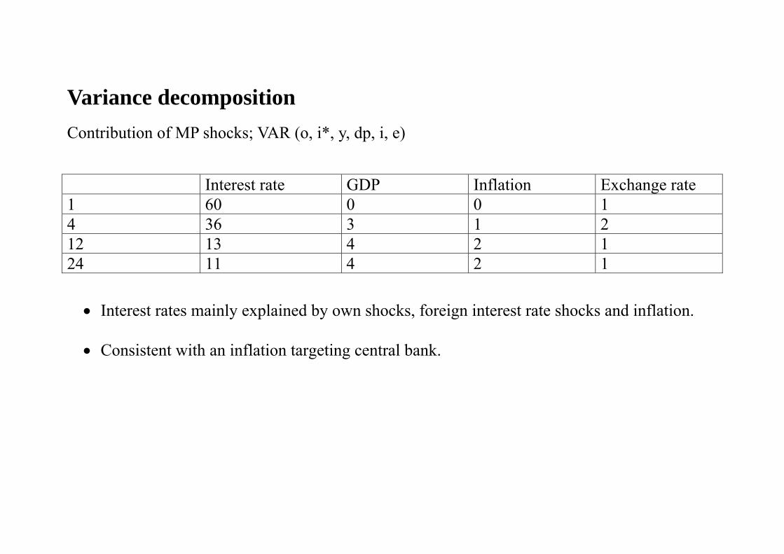
Variance decomposition Contribution of MP shocks; VAR (o, i*, y, dp, i, e)
Interest rate GDP Inflation Exchange rate 1 60 0 0 1 4 36 3 1 2 12 13 4 2 1 24 11 4 2 1
• Interest rates mainly explained by own shocks, foreign interest rate shocks and inflation. • Consistent with an inflation targeting central bank.
Empirical findings…
… using Choleski decomposition
Using the recursive Choleski restriction identifies the non-zero parameters above the interest rate equation. It turns out that the ordering of these variables does not matter for the estimated impulse responses following a monetary policy shocks. This is in line with Christiano et al., (1999; Proposition 4.1).
Results sensitive when variables are placed below the interest rate equation
Results sensitive to additional variables